advanced environmental systems analysis (aesa)home.deib.polimi.it/guariso/aesa/text.pdf ·...
TRANSCRIPT

10/6/2015
1
Advanced Environmental Systems Analysis (AESA) I.C. 10 credits
� 1st MOD: Giorgio Guariso, DEIB, Building 20,Office 2.20, 2nd floor. From Oct 5 to Nov 25Tel. 02 2399 3559, [email protected]
� 2nd MOD: Matteo Giuliani, DEIB, Building 21, Office 2.13, 2nd floor. From Nov 26 to Jan 31Tel. 02 2399 9040, [email protected]
The course is taught in the present form for the first time. About 30+30 hours lectures plus about 20+20 hours practice. Tentative program.
Advanced Environmental Systems Analysis (AESA) I.C. 10 credits
1st MOD: Models for environmental quality planning
� water quality modelling in rivers and lakes
� pollution discharge allocation
� water management for quality improvement
� integrated basin models (SWAT?)
� air pollution models (Gaussian; street canyon; Lagrangian,eulerian, particle chemical transport models)
� emission reduction plans
� health impact models
� integrated regional models

10/6/2015
2
Advanced Environmental Systems Analysis (AESA) I.C. 10 credits
2nd MOD: Decision making under global changes
� modelling demographic changes
� modelling land use changes
� modelling energy demand and resources changes
� basics of global temperature models and their outputs
� the IPCCS scenarios and their consequences
� risk and uncertainty evaluation
� decision making under uncertainty
The approach
The DPSIR scheme helps “to structure thinking about the interplay between the environment and socioeconomic activities”, and “support in designing assessments, identifying indicators, and communicating results” (EEA, 2012).

10/6/2015
3
Drivers (driving forces)
“Actions resulting from or influenced by human/natural activity or intervention”.
� Normally related to large-scale socio-economic trends� Leading to significant variations of PRESSURES� More meaningful at national/continental level than at local level� Examples: population dynamics, industrial and agricultural changes,
human mobility, climate changes,..� Often measured by variables (often called “activity levels”) describing
traffic, industries, residential heating, etc…� Inducing their changes (RESPONSE) requires extensive action and
long time (e.g. education)

10/6/2015
4
Pressures
“Discharge of pollutants into the environment”� Normally, more local phenomena linked to the specific situation of
the territory (e.g. type of agricultural, level of waste disposal services,…)
� Leading to significant variations of STATE� Often measured by variables (often called “emission levels”)
describing amount of pollutant produced and disposed into the environment
� Examples: amount of solid wastes, waste waters, fertilizer drainage, NO2 emissions from cars,…
� Inducing their changes (RESPONSE) requires both technological (e.g. new filters, new processes) and non-technological (or efficiency) changes (e.g. use bicycles instead of cars).
� Mostly evaluated indirectly (proxy variables).

10/6/2015
5
State
“Condition of different environmental compartments and systems”.
� Normally easy to measure in a single spot (monitoring)� Often measured by variables (often called “concentration”) at a
specific point in time and space, by specific gauges.� More difficult to evaluate it at a territorial level (indicator) and as an
overall environmental condition (several indicators → index)� Examples: BOD or TOC or pathogens concentration, Ozone peaks,
number of days with PM2.5 above a threshold,...� Leading to significant variations of IMPACTS� Inducing their changes (RESPONSE) requires large and expensive
technical tools (the pollutants are already in the environment) e.g. collection and treatment of wastes; aerators; PM fixing trees.

10/6/2015
6
Impact(s)
“Any alteration of conditions, adverse or beneficial, caused or induced by the variation of the state of the environment”
� Normally related to some territorial entity (NUTS 2, NUTS 3)� Requiring some kind of RESPONSE(S)� May be measured in several different ways in different sectors� Examples: number of cases, area acidified, loss of vegetation,
reduction of species, monetary damage,..� Inducing their changes (RESPONSES) may require both technical (e.g.
noise barriers along the highways) and non-technical (e.g. warning systems to reduce population exposure) actions.
P.S. A key question is “alteration with respect to what?”
Response(s) -1
“Attempts to prevent, compensate, ameliorate or adapt to changes in the state of the environment”
� They strongly depend on the structure and responsibility of the governing entities
� They may be constrained by decisions taken at higher levels (e.g. EU)� They often require some form of investment (e.g. money, learning)� Examples: impose new norms on energy in residential buildings,
establish new emission standards for cars, subsidized bio-based agriculture, build new infrastructures,…
� Can be defined using two computer-supported approaches:� Scenario based� Optimization

10/6/2015
7
Response(s) - 2
• Scenario analysis
This is the approach mainly used at the moment to design “Plans and Programs” at regional/local scale, selecting actions on the base of expert judgment and testing the effects through a suitable model of the environment. This does not guarantee that cost-effective measures are selected, and only allows for “ex-post evaluation” of costs and other impacts.
• Optimization
This approach allows for an “automatic” selection of cost-effective measures, solving an optimization model. This means that a “feedback” is provided on the “effectiveness” of the measures, in terms both of costs and of effects. To perform the optimization, one needs to embed in the overall procedure, a suitable model of the environment AND a model of the (relevant) impacts.
(Some relevant) Problems
• The policy domain does not coincide with the physical domain
Decisions that can be taken by a governing agency may be implemented in a geographical area (policy domain) quite different from the physical domain determining the environmental conditions (e.g. decision taken by a regional authority on a portion of a nation-wide river basin).
• Models can be calibrated only on past/current data
The model represents (with known accuracy) the past/present environmental conditions. Its ability in representing (new) modified conditions is unknown (representativeness). Data-based models (e.g. ARMA models) cannot be used for planning purposes: physically based models are needed, but they may be computationally very heavy (difficult to embed in an optimization procedure).

10/6/2015
8
Course topics (1st MOD)
Examples
• Determine the optimal position of a new pollutant discharge along a river
- Definition of an optimality criterion- Model of the river system- Constraints on the available locations
• Determine the least costly abatement measures to reach a given air quality in a region
- Definition of air quality- Model of the air pollution over the region- Constraints on the available technologies and their applicability

10/6/2015
9
Course topics (2nd MOD)
A dynamic view of the links
Economy/Societal dynamics
Pressure evaluation
ud(t)
decisions
A(t)
state
E(t)
output
externalconditions
vd(t) up(t)
Environmental system dynamics
Impactevaluation
E(t)
emissions
x(t)
state
y(t)
output
externalconditions
vs(t)
us(t) ui(t)
The dynamics of the first system is much slower than that of the second, thus all the variables of the first system can be considered as constant when evaluating the second.

10/6/2015
10
Data needs and expected outcome
To understand the effects of a decision, all other conditions must be known for all the relevant horizon
- The initial condition of the system must be fixed/known- All the boundary conditions must be fixed/known- The decisions must produce a significant (meaningful) change of the state- The approach is intended to compare alternatives NOT to forecast the
future (future external conditions will be different) → decision support
Environmental system dynamics
Impactevaluation
u(t)
decisions
x(t)
state
y
output
externalconditions
v(t)
Ex.
The general optimization problem (1)
Assuming:
- u(t) is the vector of decisions (values or functions)
- x(z1,z2,z3,t, u, v), where z1,z2,z3 are the spatial coordinates, is a vector (e.g. various pollutants)
- y(t) = is a vector of outputs
- The objective to be optimized J = g(y(t),u(t)) is a (small) vector
- The model of the environmental system under study is x(z1,z2,z3,t,u,v) = M(u(t),v(t))
))vu, t,,z,z,z(x(Stat 321,,, 321 tzzz
10/6/2015
11
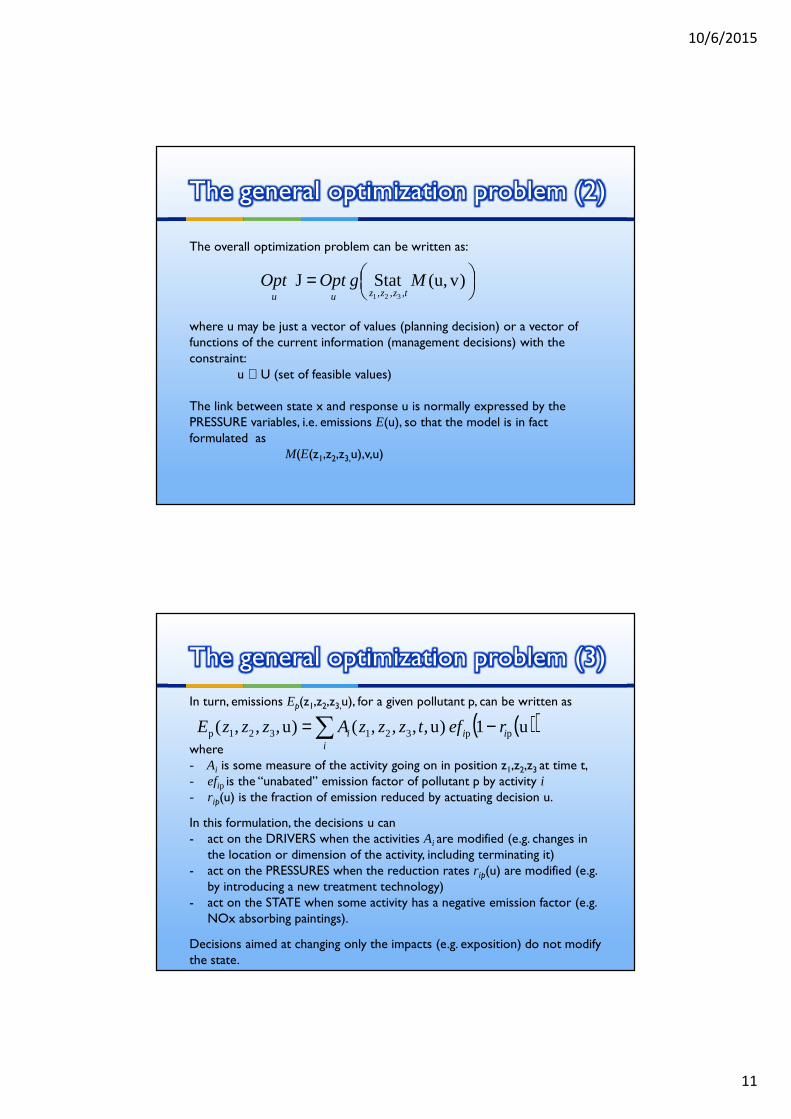
The general optimization problem (2)
The overall optimization problem can be written as:
where u may be just a vector of values (planning decision) or a vector of functions of the current information (management decisions) with the constraint:
u ∈ U (set of feasible values)
The link between state x and response u is normally expressed by the PRESSURE variables, i.e. emissions E(u), so that the model is in fact formulated as
M(E(z1,z2,z3,u),v,u)
= )v(u,StatJ
,,, 321
MgOptOpttzzzuu
The general optimization problem (3)
In turn, emissions Ep(z1,z2,z3,u), for a given pollutant p, can be written as
where - Ai is some measure of the activity going on in position z1,z2,z3 at time t, - efip is the “unabated” emission factor of pollutant p by activity i- rip(u) is the fraction of emission reduced by actuating decision u.
In this formulation, the decisions u can- act on the DRIVERS when the activities Ai are modified (e.g. changes in
the location or dimension of the activity, including terminating it) - act on the PRESSURES when the reduction rates rip(u) are modified (e.g.
by introducing a new treatment technology)- act on the STATE when some activity has a negative emission factor (e.g.
NOx absorbing paintings).
Decisions aimed at changing only the impacts (e.g. exposition) do not modify the state.
( )( )u1 )u,,,,()u,,,( pp321321p iii
i reftzzzAzzzE −=∑

10/6/2015
12
Notes
• Decisions aimed at changing only the IMPACTS (e.g. exposition) do not modify the state (represented in the previous approach by J = g(u(t),y(t)),
will not be dealt with in the course).• The objective J may depend on more than a single environmental quality
indicator/index (e.g. many different pollutants, for a list of EEA indicators: www.eea.europa.eu/publications/environmental-indicator-report-2014)
• The environmental model M also depends on the assumed external conditions v (e.g. EU legislation, climate change) that may obscure the effect of different decisions.
• Since v changes in time, the solution obtained in a given condition may not be valid time later (reliability and uncertainty).
The optimization problem is often complex (many variables, non linearity) and requires a high number of execution of the environmental model (computationally intensive).

10/6/2015
1
Environmental quality models
The most general quality model is based on the
ADVECTION – DISPERSION equation (mass balance of a pollutant C across an elementary volume dz1 x dz2 x dz3
advection(transport)
dispersion
+ chemical reactions (e.g. degradation) +
+ sources(z1,z2,z3,t) – sinks(z1,z2,z3,t)
+∂∂−
∂∂−
∂∂−=
∂∂
321
321321
),,,(
z
Cv
z
Cv
z
Cv
t
tzzzCzzz
+∂∂+
∂∂+
∂∂+
23
2
22
2
21
2
321 z
CD
z
CD
z
CD zzz
Special cases
The basic equation can be particularized in many different ways, depending on the specific problem.
Examples:• STATIONARY CONDITIONS: C does not change in time and thus
Note that the concentration may still change in space.
• DIFFUSION LOW with respect to transport
• SIGNIFICANT CHANGES only in 2D (e.g. aquifers) or 1D (e.g. rivers). Assuming the fluid direction to be z1, terms in z2 and/or z3 are disregarded.
• CHEMICAL REACTION TERM is known (e.g. null; C(t)=C0e-kt , first order kinetics)
Whatever the case, the possibility of solving the equation analytically is really rare. It must be solved with some numerical method (discretization in time AND space).
0),,,( 321 =
∂∂
t
tzzzC
0321
=== zzz DDD

10/6/2015
2
Ex. the 1-D case (river)
Consider a small, perfectly mixed volume of water, travelling along l
Sp
Ip
lba
φ(b)φ(a)
p = pollutant concentration [unit/m3]
Sp = external pollution source [unit/(m s)]
Ip = internal pollution production/depletion [unit/(m3s)]
φ = pollutant flow [unit/(m3s)]
Ex. the 1-D case (river) - 2
Mass balance (conservation) equation (law):
Sp
Ip
lba
φ(b)φ(a)
∫∫∫ ++−=∂∂ b
a p
b
a p
b
aAIS)b(A)a(ApA dldldl
tφφ
where A is the area of a volume section.

10/6/2015
3
Ex. the 1-D case (river) - 3
The mass balance equation can be rewritten using the Leibnitz theorem (inverting the order of integral and derivative) and the fundamental theorem of calculus as:
From which:
∫∫∫∫ ++∂
∂−=∂
∂ b
a p
b
a p
b
a
b
aAIS
AApdldldl
ldl
t
φ
pp AISAA +=∂
∂+∂
∂lt
p φ
φ = p v is the flow due to transport (v being the velocity)
is the flow due to diffusion along l (D being a dispersion coefficient)
l
pD
∂∂φ −=

10/6/2015
4
Note on dispersion
D takes into account:� Molecular diffusion due to the Brownian
motion of molecules (it exists also in stagnant water)
� Turbulent dispersion due to turbulent motion (macroscopic movements like eddies)
� Numerical diffusion (due to equation discretization)
Hence, it’s an empirical constant that needs calibration
Thus substituting the flow expressions, we get
which can be written
or, dividing by A,
The key point are thus: measure external load, determine internal sources/sinks (process)
Ex. the 1-D case (river) - 4
pp AISAApAp +=
∂∂−
∂∂+
∂∂
l
pDv
lt
pp AISAApA +=
∂∂−
∂∂−
∂∂+
∂∂
l
pD
ll
v
t
p
sinks sourcesppp2
2
−+∂∂+
∂∂−=
∂∂
lD
lv
t

10/6/2015
5
River models: the process
Hydraulicsubmodel
Biochemicalsubmodel
Thermalsubmodel
evaporation
flow
velocity
process heat
temperature
flowvelocity
sedimentation,water weeds
The biochemical submodel

10/6/2015
6
Simplifications
� The section is perfectly mixed� Evaporation is negligible� Process heat is negligible� Sediments and weeds do not impact the water flow� Velocity does not change temperature
Then the hydraulic and thermal sub-models can be solved independently and provide two outputs:• v(t) or v(l) and q(t) or q(l) (velocity and flow rate as function of time or
position)• T(t) or T(l) (water temperature as function of time or position)
� All the trophic chain is neglected except• The degradation of organic compounds by bacteria (using oxygen)• The presence of bacteria
Comment on the 1-D assumption
All the variables represent an average across the river cross section
PROS:
simpler model � shorter simulation time, easier parameter identification
CONS:
less accurate model � impossible to simulate unmixed sections (the model must “jump” to a well mixed section)
l z3z2l

10/6/2015
7
Comment on the 1-D assumption
Ex. The 1-D approximation cannot describe the situation of Po river at the confluence with Ticino river (in some cases the water of the two river does not mix for few hundred meters)
In stationary conditions
Q = Q(l) does not depend on time. This means the flow changes in space, but not
in time. The first de Saint Venant equation becomes:
i.e. the flow rate changes only because of discharges or abstractions. If they are measured (PRESSURES), one can compute the water balance along the river system.
Given the flow rate, one can compute the level h and the velocity v at any point
along the river through some empirical formulas, such as:
N.B. a,b,α,β are parameters to be calibrated (in general, for each section l).
dQ
dl= Sq
)l()l( )l()l( βαQhaQv b ==

10/6/2015
8
The thermal balance -1
p = Cp ρ T heat content (Cp specific heat, ρ density)
heat exchanges
The thermal balance equation has the same form with
Heat exchanges may take place:
* with tributaries/effluents* with the atmosphere* with sediments
Heat generated by internal processes is usually negligible.
SedimSurfLateralpS EEE ++=
ESedim
SurfELateralE
The thermal balance -2
Lateral heat exchanges are again computed with an energy balance:
ρpddccl CTqTQTQE )(Lateral ++−=
Outflow(per unit length)
Tributary flow rate(per unit length)
Distributed inflow(per unit length)
Tributarytemperature
Distributed inflowtemperature

10/6/2015
9
The thermal balance -3
Surface heat exchanges depend on (constant and variable) local characteristics :
• Atmospheric radiation (e.g. geographical position)* Solar radiation (e.g. cloudiness)* Reflected radiation (e.g. water temperature)* Conductance (e.g. ait temperature)* Evaporation (e.g. wind)
evapconrifsolatm IIIIIE −+−+=Surf
are difficult to evaluate. dimSurf , SeEEIn many cases, better to substitute them with a function T(l,t) derived from a set of measures taken on each reach.
Biochemical submodel
p = DO/BOD/P/N/heavy metals/…
The basic equation can be rewritten for:
The pollutant to be modelled can be:• Non-reactive (i.e. the internal sources/sinks term = 0 and only
transport and dilution are relevant)• Reactive (i.e. there are internal sources/sinks)
It may represent:• A single substance (e.g. iron, trichloroethylene) and an equation is
necessary for each substance• An aggregate indicator of various substances with similar behavior
(e.g. BOD)

10/6/2015
10
Biochemical submodel - 2
For reactive substances, a specific term must be written.For instance, for a degradable substance S, degraded by a bacterial population m, the famous Michaelis-Menten formulation is:
(it’s always a sink)
Where α1 and α2 are parameters (usually, T dependent) to be estimated in each case.
IS = − α1S
α2 + Sm
- Low values of S → degradation proportional to Sm
- High values of S →degradation proportional to m and independent on S
Biochemical submodel - 3
For- Constant (and sufficiently high) m- Low values of S
i.e. degradation is proportional to concentration
ks is again a parameter to be calibrated.
When p=DO, the internal sources/sinks are:- Reaeration (exchange with the atmosphere) - Consumption (warning: independent on DO)- Photosynthetic production: proportional to algal density)
SkmS
SI sS −≅
+−=
2
1
αα
)(2 DODOk s −...21 ++ mIS βλλ

10/6/2015
11
Temperature dependence
)20(20)( −= TT ϑθθ
T20
θ20
θ(T)
)0( <ϑ
T20
θ20
θ(T))0( >ϑ
All the previous parameters depend on temperature (some also on the flow rate).
The dependence on temperature is usually modelled through the Arrhenius formula having again two parameters:
External load
External input of pollutants may derived from a variety of sources:• Concentrated or point (tributaries, sewage discharges, industrial sources,…)• Distributed or non-point (runoff from agriculture or bare soil, rainfall,…).
In each section a mass balance equation holds.Ex. section A
The same holds for a unit volume and a non point source.
A
tribriver
tribtribriverriverA QQ
QCQCC
++=

10/6/2015
12
Streeter-Phelps model (1925)
Only 2 variables (BOD, DO) i.e. purely “chemical” model
Basic assumptions:- Degradation proportional to BOD concentration- DO consumption equal to BOD degradation- DO intake proportional to deficit- No dispersion
D
B
ukkl
vt
ukl
vt
+−+−=∂
∂+∂
∂
+−=∂
∂+∂
∂
)DODO(BODDODO
BODBODBOD
s21
1
Concentrated or distributed load
Oxygen addition (e.g. aerators, water falls,..)
Streeter-Phelps model - 2
))(0(BOD))0(DODO(DO)(DO
)0(BOD)(BOD
212
1
21
1ss
τττ
τ
τ
τkkk
k
eekk
ke
e
−−−
−
−−
+−−=
=
If we assume to move along a characteristic line, i.e. following a drop of water moving with the flow, we can rewrite the equations using the flow time τ.The dependence on l disappears.
In case of no external input, an analytical solution can be found
where BOD(0) and DO(0) are the values at the starting point.
D
B
ukkd
d
ukd
d
+−+−=
+−=
)DODO(BODDO
BODBOD
s21
1
τ
τ Linear, stationary, asymptotically stable system

10/6/2015
13
Streeter-Phelps model - 3
))(0(BOD))0(DODO(DO)(DO
)0(BOD)(BOD212
1
21
1ss
lv
kl
v
kl
v
k
lv
k
eekk
kel
el
−−−
−
−−
+−−=
=
Assuming a constant speed (at least within a certain river reach)and the two equations can be written in space instead of in flow time.
τ = l /v
l
BOD DO
BOD(0) DOs
DO(0)
l
l = 0
v
Exponential decay Combination of two exponentials (sag curve)
Streeter-Phelps model - 4
DO
DOs
DO(0)
llc
dc
One can study the DO(l) function to determine the minimum: critical deficit dc at point lc
where: d(0) is the initial deficit (DOs-DO(0)) and f = k1 / k2 is called the “autopurificationrate”.
clv
k
ef
d
fffk
vl
c
c
1)0(BOD
)0(BOD
)0(d)1(1ln
)1(1
−
=
−−−
=
This means:- The critical deficit increases with BOD(0)- The critical distance decreases with the initial deficit and initial BODNote: BOD values are order of tens, hundreds; DO values are order of units

10/6/2015
14
Streeter-Phelps model (+ & -)
PLUS:- Very simple: easy to compute and calibrate (two parameters)- Linear: the superposition principle holds (the effect of two inputs at two
different locations, may be computed separately and then added)
MINUS:- For high values of BOD (initial and/or load) the computed DO concentration
becomes negative (unfeasible). This means that the degradation process becomes different (anaerobic) and this is not represented in the model
- In a “clean” river, the bacteria population may not be ready to decompose the incoming BOD and thus the real degradation is slower.
River network
To apply the model in practice, one has to subdivide the river network in a set of elementary units (reaches) that can be considered homogeneous as to:- Flow- Velocity- Temperature- Non-point loadsAt each confluence a mass balance equation must be written.

10/6/2015
15
Model use
� Determine the minimum treatment cost C(w) of the discharge w at a given point to guarantee a minimum DO value DO
C(w) subject to DO(l) ≥ DO ∀ 0 ≤ l ≤ L
� Determine the best position to discharge a given load to maximize a water quality index W(BOD(l),DO(l))
W(BOD(l),DO(l)) subject to 0 ≤ l ≤ L
� Determine the value of the unmeasured load w at point l, given a set of actual concentration measures BODi, DOi at points li.
subject to w ≥ 0.
This is an inverse problem, known as “source apportionment”.
wmin
lmax
( ) ( )[ ]∑ −−+−i
2ii
2ii
wDO)l(DO)1(BOD)l(BODmin αα
Model use - 2
Input values (decisions, external conditions) are often (always?) known only numerically (data, assumptions). The analytical solution of model equations is not possible → simulation
For simulation to be useful for decision-making:
• The model must work “around” a stable attractor
L l
t
Tdepends on boundary conditions (including inputs)
depends on initial conditions
Simulation domain
initial conditions
upstream and downstream boundary conditions
When D>0 (non negligible dispersion) the time to forget initial conditions it’s longer (backward effect).

10/6/2015
16
Model use - 3
• The numerical scheme for integration of equations must be stable
The stability of a forward difference scheme for PDE is granted if the CFL (Courant-Friedrichs-Lewy) condition holds:
= Courant number <1
It means that the time discretization (time step) must be small with respect to the space discretization (in a time step the flow must travel less that a space step)
• The model must work “around” the values used for validation, but
• The input changes must have a perceivable effect on the output
• The external conditions must be representative for the decision criterion (average, extreme,…)
• The calculation must be fast enough to be repeated may times.
vl
tCr ∆
∆=
A more refined model (Stehfest)
Assumptions:• Negligible diffusion• No algae, no sediments (deep river)• Slow fish dynamics (hence, negligible)• Two BOD species: slowly and rapidly degradable
State variables:- w1 rapidly degradable BOD- w2 slowly degradable BOD- B bacteria- P protozoa- DO oxygen
All concentrations in g/m3

10/6/2015
17
A more refined model - 2
Pollutant dynamics (external input = 0)
dw1
dτ= −k11
k31w1
k32 + w1
B
dw2
dτ= −k21
k33w2
k34 + w2 + k35w1
Bw1
k31B
Michaelis-Menten(B is relevant)
Competitive inhibition: if w1 is large, degradation of w2 is slowerIf w1 is small, degradation follows M-M
For highly polluted rivers (high values of w1 and w2 and constant B, we go back to S-P model.
When the motion law of the flow is known, the equations can be again written in terms of spatial distance from the origin.
dB
dτ= k31w1
k32 + w1
+ k33w2
k34 + w2 + k35w1
− k36
B − k37
k41B
k42 + BP
dP
dτ= k41B
k42 + B− k43
P
A more refined model - 3
Bacteria and protozoa (external input = 0)
predation by protozoagrowth due to BOD consumption
mortality
mortality
growth due to predation of bacteria
Many parameters to estimate/evaluate.Oxygen does not enter the equations (same problem as S-P for anoxic conditions).

10/6/2015
18
A more refined model - 4
Pollutant dynamics (external input = 0)
dw1
dτ= −k11
k31w1
k32 + w1
B
dw2
dτ= −k21
k33w2
k34 + w2 + k35w1
Bw1
k31B
Michaelis-Menten(B is relevant)
Competitive inhibition: if w1 is large, degradation of w2 is slowerIf w1 is small, degradation follows M-M
For highly polluted rivers (high values of w1 and w2 and constant B, we go back to S-P model.
When the motion law of the flow is known, the equations can be again written in terms of spatial distance from the origin.
PkBk
Bkk
Bkwkwk
wkk
wk
wkk
kd
d
+
+−
+
+
+++
+−
+−=
5642
4155
54135234
23353
132
13152
s51
)DODO(DOτ
A more refined model - 5
Oxygen dynamics reoxygenation from the atmosphere
consumption by degradation and respiration processes
consumption by predation and respiration of protozoa

10/6/2015
19
Application to a real case
The Rhine river in Germany (about 500 km)
Subdivided into 12 reaches (mainly divided by tributaries) with constant flow (MQ) and lateral inflow, and constant distributed loads.
The Rhine river case
The loads are measured as COD and thus only a portion α (a parameter to be estimated) can be degraded by bacteria.
Streeter-Phelps simulation
The Streeter-Phelps model cannot represent the last reaches of the river

10/6/2015
20
The Rhine river case - 2
Stehfest model simulation
There is only a marginal improvement, especially in the first reaches, to represent the actual measurements.
w1, w2, and w3 (non degradable part) are the three components of COD.
Note also that these are the CALIBRATION results. No validation has been possible due to lack of data.
However…
Rhine development plans
Let’s imagine that we want to optimally allocate new loads along the main river stream.
First, we have to define a suitable optimality indicator:
e.g. the integral of the oxygen deficit
The S-P solution
( )∫ −= fin
o
l
ldllJ s1 DO)(DO
Almost all the new load is moved toward the end of the German stretch since, in this way, most of the deficit is produced in Holland.
old
new

10/6/2015
21
Rhine development plans - 2
With the Stehfest model results are different:
The new load is spread more regularly along the river and the oxygen concentration toward the end is even better than with less load!
This apparent contradiction may be explained looking at the dynamics of bacteria.
old
new
old
new
The higher bacterial population in the central reach (Rhine Valley) allows a more regular oxygen consumption.
Rhine development plans - 3
The plan objective, though referring to the entire river (not just a spot value) does not take sufficiently into account the effects in the Netherland.
It is necessary to somehow evaluate the terminal condition (common problem). One possibility is to add a component of the objective based on the deficit at the border (final oxygen demand or FOD).
The new objective term may have the form:
where FOD* is a limit (untouchable) value. For low valued of FOD* the new load spreads from upstream to downstream, while for high value, the new load goes upstream only because of lack of space.
FOD*FOD
FOD2 −
=J

10/6/2015
22
Current models
Starting from the original equations many implementations have been developed mainly different for data handling and connections to GISs.
From US EPA (http://www.epa.gov/athens/wwqtsc/):
WASP – Water
Quality Analysis Simulation Program
SWMM (Storm
Water Management Model)BASINS
EPD-RIV1One Dimensional Riverine Hydrodynamic and Water Quality Model
QUAL2K
Development began in 1987 (Brown and Barnwell).
By far, the most famous and used water quality model:
• One dimensional.: The channel is well-mixed vertically and laterally• Steady state hydraulics: Non-uniform, steady flow• Diurnal heat budget and temperature simulated as a function of meteorology • Diurnal water-quality kinetics • Heat and mass inputs: Point and non-point loads and abstractions
PLUS• Carbonaceous BOD speciation (two forms, slow and fast) • Anoxia: Q2K reduces oxidation reactions to zero at low oxygen levels• Sediment-water interactions and bottom algae• Light extinction• pH• Pathogens
NOTE: latest implementation (2009) in Excel (originally FORTRAN)

10/6/2015
23
QUAL2K - 2
The Arno river and the Q2K scheme
Simulation of temperature and coliforms (importance of the selection of the hydraulic regimes)
An uncertainty (Monte Carlo) analysis is possible
QUAL2K - 3
Q2K can reproduce weirs and other hydraulic discontinuities.
Each reach is simulatedas a trapezoidal channel using Manning’s equation

10/6/2015
24
QUAL2K -4
Up to 14 components. Daily input patterns.
Simulated processes
dn
upipo
h
e
d
s
s
s
sodcf
re
se
se se
se
s
smi
s
Alk
s
X
hnano
nnn
cf
hcs
oxox
mo
dsrod
rda
rna
rpaIN
IPa
p
r
s
u
e
o
cT
ocT
o
cT
o
cT
o
cT
dn
upipo
h
e
d
s
s
s
sodcf
re
se
se se
se
s
smi
s
Alk
s
X
hnano
nnn
cf
hcs
oxox
mo
dsrod
rda
rna
rpaIN
IPa
p
r
s
u
e
o
cT
ocT ocT
o
cT
o
cT
o
cT
CARBON
NITROGEN
PHOSPHORUSOrganic Inorganic
Organic Ammonia Nitrate
Detritus Slow Fast Tot. inorganic
Oxygen
Algae
Integrated model: SWAT
“Soil and Water Assessment Tool” – joint study of soil use and water quality
Developed by USDA, since 1980’s Deterministic, physically based, DISTRIBUTED model (time step = 1 day) Manual: 649 pages (2009), Conferences, User Groups.
• Used for long-term studies: Assesses impacts of climate and land management on yields of water, sediment, and agricultural chemicals
• Includes hydrology, soil temperature, plant growth, nutrients, pesticides and land management
• Uses a spatial discretization called Hydrologic Response Unit (HRU)

10/6/2015
25
SWAT - 2
Land Use layer Soils layer
+ + …
A HRU is a unique combination of soil characteristics (slope, exposition, activities, rainfall,…) that are assumed constant within the unit → GIS operations → ArcSWAT
SWAT - 3

10/6/2015
26
SWAT – 4 (ex. : water in soil)
SWAT separates soil profiles into 10 layers to model inter and intra-movement between layers. The model is applied to each soil layer independently starting at the upper layer.
SWAT soil water routing feature consists of four main pathways:1. soil evaporation2. plant uptake and transpiration3. lateral flow4. percolation.
• Storage routing technique combined with a crack-flow model to predict flow through each soil layer
• Cracked flow model allows percolation of infiltrated rainfall though soil water content is less than field capacity.
• Portion that does become part of layer stored water cannot percolate until storage exceeds field capacity.
SWAT – Example GAC, Ethiopia
The Gilgel Abay Catchment (5000 km2) isthe largest of the four main sub-catchmentsof Lake Tana, Ethiopia
Blue Nile source

10/6/2015
27
DEM 30mx30m data: 58% falls between 0-8% slope and 4% with steep slope>30% mainly in the southeast part.
DATA -1
Agriculture (around 65%) is the dominant land use in the catchment while agro-pastoral accounts 33% of the land uses , 1% is agro-forestry and 0.1 % urban.
DATA - 2
Rainfall and temperature data (outside the basin), flow data in Merawi
0,00
5,00
10,00
15,00
20,00
25,00
30,00
35,00
T(o
c)
days
Maximum tempMinimum temp

10/6/2015
28
Model formulation
• Surface runoff computation: SCS curve number procedure, where the curve number varies with antecedent soil moisture, land cover, soil permeability
• Soil loss was calculated using MUSLE (modified soil loss equation) method which uses a runoff factor that accounts for the energy used in detaching and transporting of sediment, in addition to parameters related to land cover, soil erodibility, topographic factor & support practice factor
• SWAT allows to apply agricultural management practices (tillage, planting and growing, fertilization, irrigation …) on selected HRU
• The model assumes surface runoff interacts with the top 10mm of soil. Nutrients contained in this layer are available for transport to the main channel in the surface runoff
• The fertilization operation allows the user to specify the fraction of fertilizer that is applied to the top 10mm.
Model formulation - 2
10/6/2015
29
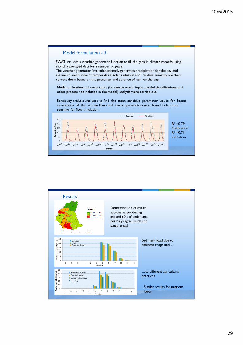
Model formulation - 3
SWAT includes a weather generator function to fill the gaps in climate records using monthly averaged data for a number of years.The weather generator first independently generates precipitation for the day and maximum and minimum temperature, solar radiation and relative humidity are then correct them, based on the presence and absence of rain for the day.
Model calibration and uncertainty (i.e. due to model input , model simplifications, and other process not included in the model) analysis were carried out
Sensitivity analysis was used to find the most sensitive parameter values for better estimations of the stream flows and twelve parameters were found to be more sensitive for flow simulation.
R2 =0.79CalibrationR2 =0.71validation
Results
Determination of critical sub-basins, producing around 60 t of sediments per ha⋅y (agricultural and steep areas)
0
10
20
30
40
50
1 2 3 4 5 6 7 8 9 10 11 12
Sed
imen
t yie
ld(t
/ha)
Months
Soya beanLentilGrain sorghum
Sediment load due to different crops and…
…to different agricultural practices
0
10
20
30
40
50
1 2 3 4 5 6 7 8 9 10 11 12Sed
imen
t Y
ield
(t/h
a)
Months
Mould board plow
Field Cultivator
Conservation tillage
No tillage
Similar results for nutrient loads.

10/6/2015
30
Policy indications
0
10
20
30
40
50
60
70
80
90
0 20 40 60 80 100
perc
en
t in
cre
ase
percent increase of fertilization
Nitrate yield
Crop yield
Increased fertilization increases proportionally N load without a similar increase in yield
A decrease of cultivated area by 20% results in a decrease in sediment yield of more than by 50%.
Mould board plow tillage and Field cultivator tillage increase sediment yield by 26.6% and 2% compared to generic conservation tillage. But Field cultivator reduces sediment yield by 25% wrt conventional tillage practice
Avoiding tillage (no tillage) practice is even better for sediment yield (-25%)
Flow rate decreases by 0.4% in soybean cultivation as compared to Grain sorghum
Grain sorghum, with field cultivator and low fertilizer dose (50%) is a recommended practice getting both low sediment and nutrient release with good yield.

10/6/2015
1
Lake (deep) models
The basic difference with rivers is that the horizontal dimension(s) are comparable to depth. Thus:• The velocity of the water is small (negligible)• The differences along the vertical dimension are relevant• The dynamics of higher levels of the trophic chain (phytoplankton,
zooplankton, fishes) are relevant• Slower processes (e.g. seasonal changes) must be considered• The underlying hydraulic model is obviously different
A lake (often artificial) can be studied as a sequence of horizontally perfectly mixed boxes.
Stratification
The basic consequence of depth (in temperate climate) is water stratification.
springwind
� heating faster than mixing
summer
same temp. thus mixing
warm water is less dense, thus floats, and needs lots of wind to mix

10/6/2015
2
Stratification - 2
Stratified lakes present three distinct zones.
thermocline
dept
h (m
)
temperature (°C)0 10 3020
0
10
30
20
region of rapid temperature change
hypolimnium
epilimnium
sediments
Eutrophication

10/6/2015
3
Eutrophication consequences
Loss of water quality, fish death
Eutrophication processes (WASP7)
Phytoplankton
NH3
Respiration
Dis.
Org. P
Dis.
Org. NCBOD1
CBOD2
CBOD3
PO4
SSinorg
Settling
Photosynthesis
Denitrification
Nitrification
atmosphereDO
NO3
Adsorption
Oxidation
Mineralization
Reaeration
N
NPC
Detritus
Periphyton
Death&Gazing

10/6/2015
4
Phytoplankton
� The growth rate of a population of phytoplankton in a natural environment:
� is a complicated function of the species of phytoplankton present
� involves differing reactions to solar radiation, temperature, and the balance between nutrient availability and phytoplankton requirements
� Due to the lack of information to specify the growth kinetics for individual algal species all models characterizes the population as a whole by the total biomass of the phytoplankton present (measured in terms of chlorophyll concentration)
Phytoplankton - 2
Phyt
NO3
PO4
NH3 O C:N:P
Light
NLTG XXXGR max=Growth rate:
Gmax = maximum specific growth rate constant at 20 C, 0.5 – 4.0 day-1
XT = temperature growth multiplier , dimensionless
XL = light growth multiplier, dimensionless
XN = nutrient growth multiplier, dimensionless

10/6/2015
5
Phytoplankton growth
where: θG = temperature correction factor for growth (1.0 – 1.1)T = water temperature, °C
20−= TGTX θ Temperature multiplier
++= ,...,min
pp
p
NiNi
NiN CK
C
CK
CX
Nutrient multiplier
Defines a limiting factor
KMN
semisaturationconstant
Phytoplankton growth - 2XL depends on the light l(z) available for photosynthesis at depth z. It may be
written using Michaelis-Menten formulation
or Steele (1965) formulation
where ls represents an optimal (maximum) light intensity.
But
• The incident light on a water surface varies during the day and the season
• The light intensity naturally decreases with depth
• The presence of phytoplankton further increases light attenuation (self-shadowing)
)(
)()(
zlk
zlzX
lL +
−=
−−=
ssL l
zl
l
zlzX
)(1exp
)()(

10/6/2015
6
Light attenuationThe light intensity dependence on depth l(z) can be expressed by the Beer-
Lambert law
where l0 is the incident radiation on the surface and the function
can be written as a polynomial function of phytoplankton concentration.
))(exp()( 0 zPhytlzl γ−=)(Phytγ
Typical seasonal patterns
The relation between phytoplankton and zooplankton is a typical predator-prey system.Algal blooms occur in spring.

10/6/2015
7
Death rate:
)(1120
11 tZkkkR GDTRRD ++= −θ
k1R = endogenous respiration rate constant, day-1
θ1R = temperature correction factor, dimensionless
k1D = mortality rate constant, day-1
k1G = grazing rate constant, day-1, or m3/gZ-day if Z(t) specified
Z(t) = zooplankton biomass time function, gZ/m3 (defaults to 1.0)
Other components of phyoplankton dynamics
Settling rate:
VAvR SSS /=
vS = settling velocity, m/day
AS = surface area, m2
V = segment volume, m3
Phosphorus cyclePhytoplankton
4PO4 Org. P
20 483 83 8
4
T
mpc
Ck C
K Cθ −
+
Detr. P
� Phytoplankton P
� Detrital P
4 44
pc sp p pc
C a vG D C a
t D
∂ = − − ∂ Growth
Death
Settling
D
vCkCafD
t
C sTdissdisspcOPp
1515
204
15 −−=∂
∂ −θ
SettlingDeathDeath Dissolution
203 3 344 83 83 8 4 3
4
(1 )(1 ) T s d
p op pc p pcmpc
C v fCD f a C k C G C a C
t K C Dθ −∂ −
= − + − −∂ +
SettlingMineralization GrowthDeath
84
420838315
208 CCK
CkCk
t
C
mpc
TTdissdiss
+−=
∂∂ −− θθ
MineralizationDissolution
� Inorganic P
� Dissolved organic P

10/6/2015
8
Very high number of parameters
Difficult to calibrate for a specific situation.
Ex. Phosphorus cycle parameters
Fully distributed model
It is necessary to compute all the internal processes for each volume in a grid and model the dispersion exchanges with the surrounding volumes (thousands of state variables)

10/6/2015
9
Control of eutrophication
� Reduce loads (less use of detergents or fertilizers, better treatment,…)
� Artificial mixing
� Selective discharges
� Artificial aeration
Epilimnio
Pro
fon
dità
(7
,5 m
)
Ipolimnio
Pro
fon
dità
(1
0 m
)
Superficie totale (4933000 m2)
Defining the planning/control problem
An aggregated (time and space) quality indicator is necessary

10/6/2015
10

10/6/2015
11

10/6/2015
12