Advanced Econometrics

Week 3

Institute of Economic StudiesFaculty of Social Sciences

Charles University in Prague

Fall 2015

1 / 31

Outline of Today’s talk

Last week, we have introduced (broadly) main estimationtechniques.

Following weeks, we will look at the main ones in detail.

Today, we will discuss the principles of MaximumLikelihood Estimation (MLE).

MLE is the most widely used estimation technique due toits properties.

Today, we will see why.

2 / 31

Motivation

We only cared about the conditional mean → the mostprobable value given x.

We estimated the parameters by minimizing the variance ofthe residuals.

This is equivalent to maximizing the R2, or maximizing thesimilarity between what we observe and what our modelpredicts.

In other words, we maximize the probability that theexpected values are the observations.

In the Maximum Likelihood, we also maximize thesimilarity.

But we do it by maximizing the probability of y.

3 / 31

Motivation cont.

MLE defines a class of estimators based on the assumptionon particular distribution about the observed randomvariable.

If it is safe making this assumptions, MLE is generally veryattractive (also for non-linear models.)

The main advantage is that among all consistentasymptotically normal estimators, MLEs have optimalasymptotic properties.

The main disadvantage is that they are not necessarilyrobust to failures of the distributional assumptions made.

4 / 31

The Likelihood Function

The pdf for a random variable y conditioned on theparameters θ is f(y|θ).

f(y|θ) identifies the data-generating process that underliesthe observed sample.

f(y|θ) also describes the data that the process will produce.

The joint probability of n i.i.d. observations from thisprocess is

f(y1, . . . , yn|θ) =

n∏i=1

f(yi|θ) = L(θ|y)

The joint density is the likelihood function defined as afunction of:

θ′ = (θ1, . . . , θK), K-dimensional set of unknownparametersy′ = (y1, . . . , yn) collection of sample data

5 / 31

The Log-Likelihood Function

Note that the L(θ|y) is function of parameters conditionalon data, but is equivalent to L(y|θ).

Logarithm is a monotone and increasing transformationwhich transforms products of the pdf into the sums:

ln L(θ|y) =

n∑i=1

ln f(yi|θ)

We call this log-likelihood function.

Note that f(yi|θ) is contribution of i-th observation to thelikelihood.

6 / 31

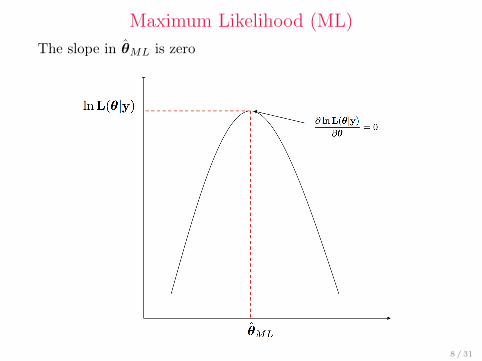
Maximum Likelihood (ML)

ML ⇒ to maximize a likelihood:

θML = argmaxθ

ln L(θ|y)

Score:∂ ln L(θ|y)

∂θHessian:

∂2 ln L(θ|y)

∂θ∂θ′

The hessian is important for computing asymptoticvariance of the estimator, as we will see later.

The MLE of θ is setting the score to zero:

∂ ln L(θ|y)

∂θ= 0

The slope in θML is zero (FOC for maximization)

7 / 31

Maximum Likelihood (ML)

The slope in θML is zero

8 / 31

Identification

Even before we begin estimation, we need to ask a questionof whether estimation of the parameters is possible ⇒ thequestion of identification.

The issue of identification must be resolved beforeestimation (for consistency).

Can we uniquely determine the values of θ from thesample?

Definition 1: Identification

The parameter vector θ is identified (estimable) if for anyother parameter vector θ∗ 6= θ, for some data y,

L(θ∗|y) 6= L(θ|y)

This result is crucial for the estimation9 / 31

Example

Let y ∼ N(θ, 1),then the likelihood is

L(θ|y) =

n∏i=1

f(yi|θ) =1

(2π)n/2exp

(−1/2

n∑i=1

(yi − θ)2)

Taking logs and computing the score:

∂ lnL(θ|y)

∂θ= 0

Impliesn∑i=1

(yi − θ) = 0

Hence θLM = 1/n∑n

i=1 yi = y

10 / 31

Properties of MLE

MLEs are most attractive because of their large sampleasymptotic properties.

Consistent: not necessarily unbiased, however

Asymptotically normally distributed

Asymptotically efficient: among the possible estimatorsthat are consistent and asymptotically normally distributed(coutrerpart to Gauss-Markov for linear regression).

Invariant: The MLE of g(θ) is g(the MLE of θ)

11 / 31

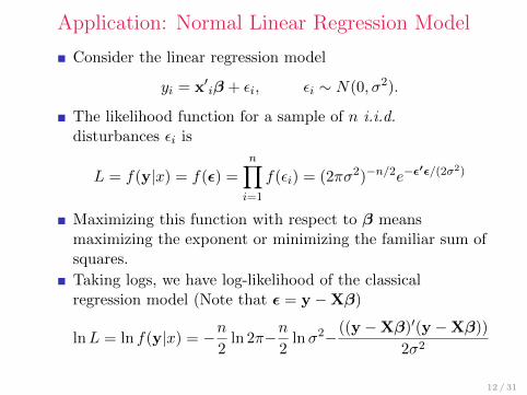
Application: Normal Linear Regression Model

Consider the linear regression model

yi = x′iβ + εi, εi ∼ N(0, σ2).

The likelihood function for a sample of n i.i.d.disturbances εi is

L = f(y|x) = f(ε) =

n∏i=1

f(εi) = (2πσ2)−n/2e−ε′ε/(2σ2)

Maximizing this function with respect to β meansmaximizing the exponent or minimizing the familiar sum ofsquares.

Taking logs, we have log-likelihood of the classicalregression model (Note that ε = y −Xβ)

lnL = ln f(y|x) = −n2

ln 2π−n2

lnσ2−((y −Xβ)′(y −Xβ))

2σ2

12 / 31

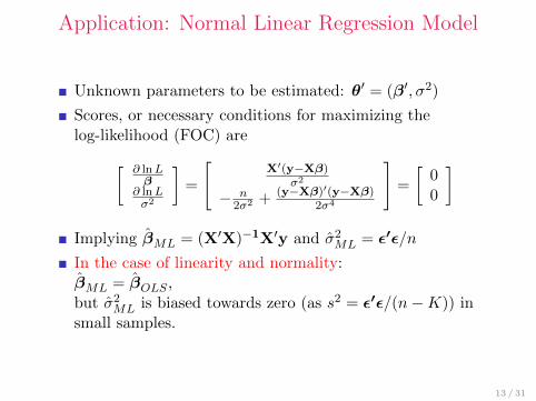
Application: Normal Linear Regression Model

Unknown parameters to be estimated: θ′ = (β′, σ2)

Scores, or necessary conditions for maximizing thelog-likelihood (FOC) are[ ∂ lnL

β∂ lnLσ2

]=

[X′(y−Xβ)

σ2

− n2σ2 + (y−Xβ)′(y−Xβ)

2σ4

]=

[00

]

Implying βML = (X′X)−1X′y and σ2ML = ε′ε/n

In the case of linearity and normality:βML = βOLS ,but σ2ML is biased towards zero (as s2 = ε′ε/(n−K)) insmall samples.

13 / 31

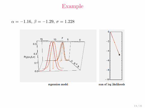
Example

α = −1.16, β = −1.29, σ = 1.228

14 / 31

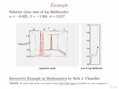
Example

Solution (max sum of log likelihoods):α = −0.825, β = −1.301, σ = 0.217

Interactive Example in Mathematica by Seth J. Chandler.(NOTE: To make this work, you need to have Free CDF player installed on your computer.)

15 / 31

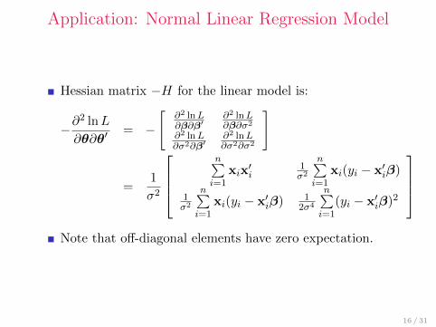
Application: Normal Linear Regression Model

Hessian matrix −H for the linear model is:

−∂2 lnL

∂θ∂θ′= −

[∂2 lnL∂β∂β′

∂2 lnL∂β∂σ2

∂2 lnL∂σ2∂β′

∂2 lnL∂σ2∂σ2

]

=1

σ2

n∑i=1

xix′i

1σ2

n∑i=1

xi(yi − x′iβ)

1σ2

n∑i=1

xi(yi − x′iβ) 12σ4

n∑i=1

(yi − x′iβ)2

Note that off-diagonal elements have zero expectation.

16 / 31

Application: Normal Linear Regression Model

Information matrix:

I(θ) = −E[H] =

1σ2

n∑i=1

xix′i 0′

0 n2σ4

Does this look familiar?

By taking inverse, we obtain asymptotic variance

I(θ)−1 =

[σ2(X′X)−1 0′

0 2σ4

n

]

17 / 31

Properties of an MLE

MLEs are most attractive because of their large sampleasymptotic properties.

Theorem 1 Properties of an MLE

1 Consistency: plim θMLE = θ0

2 Asymptotic normality: θMLEa∼ N

(θ0, I(θ0)

−1), whereI(θ0) = −E0[∂

2 lnL/∂θ0∂θ′0] is the Fisher Information

matrix.

3 Asymptotic efficiency: θMLE is asymptotically efficientand achieves the Cramer-Rao lower bound forconsistent and asymptotically normally distributedestimators.

4 Invariance: The MLE of γ0 = c(θ0) is c(θMLE) if c(θ0)is a continuous and continuously differentiable function.

18 / 31

Properties of an MLE

For this theorem, we need to assume that

(y1, . . . , yn) is a random sample from the population withdensity function f(yi|θ0)and that the following regularity condition hold (notethat the statement is rather informal).

Definition 2 Regularity Conditions

1 The first three derivatives of ln f(yi|θ) wrt θ arecontinuous and finite for almost all yi and for all θ.

2 The conditions necessary to obtain the expectations of thefirst and second derivatives of ln f(yi|θ) are met.

3 For all values of θ, |∂3 ln f(yi|θ)/∂θj∂θk∂θl| is less than afunction that has finite expectation.

19 / 31

Asymptotic Variance

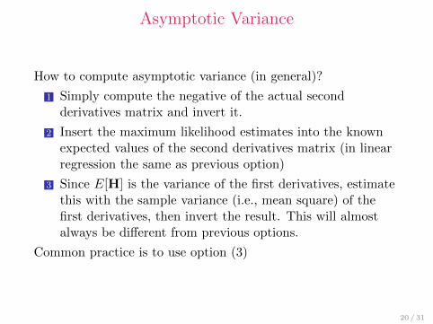
How to compute asymptotic variance (in general)?

1 Simply compute the negative of the actual secondderivatives matrix and invert it.

2 Insert the maximum likelihood estimates into the knownexpected values of the second derivatives matrix (in linearregression the same as previous option)

3 Since E[H] is the variance of the first derivatives, estimatethis with the sample variance (i.e., mean square) of thefirst derivatives, then invert the result. This will almostalways be different from previous options.

Common practice is to use option (3)

20 / 31

Properties of an MLE

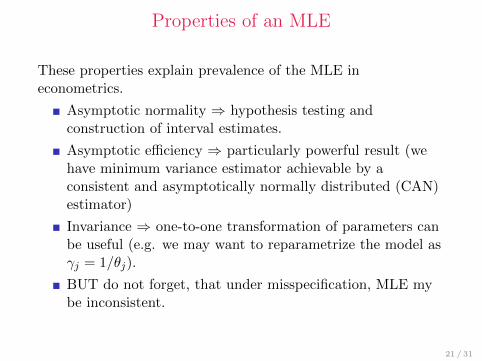
These properties explain prevalence of the MLE ineconometrics.

Asymptotic normality ⇒ hypothesis testing andconstruction of interval estimates.

Asymptotic efficiency ⇒ particularly powerful result (wehave minimum variance estimator achievable by aconsistent and asymptotically normally distributed (CAN)estimator)

Invariance ⇒ one-to-one transformation of parameters canbe useful (e.g. we may want to reparametrize the model asγj = 1/θj).

BUT do not forget, that under misspecification, MLE mybe inconsistent.

21 / 31

Conditional likelihood

While these results form a statistical theory for the MLE,we are missing crucial element.

We analyzed mostly the case of the density of an observedrandom variable and a vector of parameters, (fi|θ).

But we need to include exogenous variables xi.

The joint density of yi and xi will form the log-likelihood

lnL(θ, δ|data) =

n∑i=1

ln f(yi,xi|α)

=

n∑i=1

ln f(yi|xi,θ) +

n∑i=1

ln g(xi|δ)

With α holding [θ, δ] parameters to be estimated.

22 / 31

Conditional MLE

Asymptotic results for the maximum conditional likelihoodestimator must account for xi.

Under well-behaved data, the sample will average such as

(1/n) lnL(θ|y,X) =1

n

n∑i=1

ln f(yi|xi,θ)

To establish the asymptotic properties, let’s think aboutthis as a general extremum estimator.

An extremum estimator is one obtained as theoptimizer of a criterion function q(θ|data).

A criterion function for obtaining the θMLE islog-likelihood (for θOLS estimate it was sum of squareerrors).

23 / 31

Assumptions for Asymptotic Properties

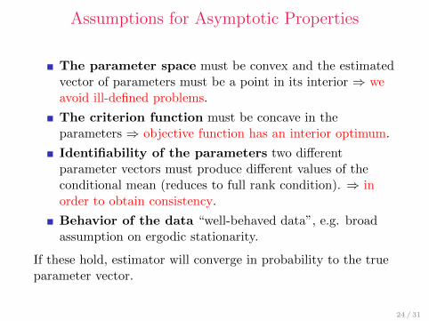
The parameter space must be convex and the estimatedvector of parameters must be a point in its interior ⇒ weavoid ill-defined problems.

The criterion function must be concave in theparameters ⇒ objective function has an interior optimum.

Identifiability of the parameters two differentparameter vectors must produce different values of theconditional mean (reduces to full rank condition). ⇒ inorder to obtain consistency.

Behavior of the data “well-behaved data”, e.g. broadassumption on ergodic stationarity.

If these hold, estimator will converge in probability to the trueparameter vector.

24 / 31

Asymptotic Properties

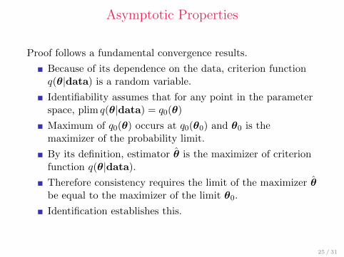
Proof follows a fundamental convergence results.

Because of its dependence on the data, criterion functionq(θ|data) is a random variable.

Identifiability assumes that for any point in the parameterspace, plim q(θ|data) = q0(θ)

Maximum of q0(θ) occurs at q0(θ0) and θ0 is themaximizer of the probability limit.

By its definition, estimator θ is the maximizer of criterionfunction q(θ|data).

Therefore consistency requires the limit of the maximizer θbe equal to the maximizer of the limit θ0.

Identification establishes this.

25 / 31

Asymptotic Properties

Theorem 2: Asymptotic Normality of M Estimators

If

θ is a consistent estimator of θ0, where θ0 is a point in theinterior of the parameter space;

q(θ|data) is concave and twice continuously differentiablein θ in a neighbourhood of θ0;√n[∂q(θ0|data)/∂θ0]

d→ N(0,Φ);

for any θ in Θ,limn→∞ Pr[|(∂2q(θ|data)/∂θk∂θm)− hkm(θ)| > ε] = 0for all ε > 0, where hkm(θ) is a continuous finite valuesfunction of θ;

the matrix of elements H(θ) is nonsingular at θ0, then

√n(θ − θ0)

d→ N(0,H−1(θ0)ΦH−1(θ0)

)26 / 31

Quasi ML (QML)

If we are only interested in the conditional meanparameter, there is a way to estimate them consistentlyeven if the assumed density is not correct.

This is Pseudo ML (PML) or Quasi ML (QML).

The idea is that certain family of densities whose FOC(score) wrt. parameters in the mean are exactly the same.

Exponential family: Gaussian, Exponential, Poisson,Bernoulli, Binomial and their multivariate versions.

27 / 31

Asymptotic distribution of QML

The asymptotic distribution of the QML estimator differsfrom the ML.

Here, we need to use a so-called sandwich

√n(θQML − θ0)

d→ N(0, I−1(θ0)J (θ0)I−1(θ0)

)I(θ0) holding negative expectations of Hessian matrix.

J (θ0) holding expectation of the first derivatives of thelog-likelihood function wrt parameters.

Current trend is to use this sandwich, as it is robust evenfor the MLE.

If the log-likelihood is correct, sandwich simplifies toI−1(θ0)

28 / 31

MLE

So why not always use MLE with all the attractiveproperties?

Efficiency comes at the price of non robustness.

If some part of assumed distribution is misspecified, MLEis inconsistent.

It is desirable to make as few assumptions as possible.

Still, MLE plays central role in modern econometrics, andfor many problems, it is essential.

29 / 31

Testing Hypotheses - Three Tests

To test the restrictions on parameters, we commonly use:

The likelihood ratio test

lnLU – log-likelihood without restrictions on parameters.lnLR – log-likelihood with restrictions.lnLU > lnLR for any nested restrictions.2(lnLU − lnLR) ∼ χ2

j , with j restrictions.Practical shortcoming is that we need to estimate bothrestricted and unrestricted versions of the model.

The Wald test

The Lagrange multiplier test

30 / 31

Thank You For Your Attention

Reading

This (third) week Ch. 14 (MLE) pp. 509 - 548

Next (fourth) week Ch. 13 (GMM) pp. 455-480

31 / 31