advanced difference of convex functions algorithms for
TRANSCRIPT
HAL Id: tel-02557281https://hal.univ-lorraine.fr/tel-02557281
Submitted on 28 Apr 2020
HAL is a multi-disciplinary open accessarchive for the deposit and dissemination of sci-entific research documents, whether they are pub-lished or not. The documents may come fromteaching and research institutions in France orabroad, or from public or private research centers.
L’archive ouverte pluridisciplinaire HAL, estdestinée au dépôt et à la diffusion de documentsscientifiques de niveau recherche, publiés ou non,émanant des établissements d’enseignement et derecherche français ou étrangers, des laboratoirespublics ou privés.
Advanced Difference of Convex functions Algorithms forsome topics of Machine Learning with Big Data
Bach Tran
To cite this version:Bach Tran. Advanced Difference of Convex functions Algorithms for some topics of Machine Learningwith Big Data. Computer Science [cs]. Université de Lorraine, 2019. English. NNT : 2019LORR0255.tel-02557281

AVERTISSEMENT
Ce document est le fruit d'un long travail approuvé par le jury de soutenance et mis à disposition de l'ensemble de la communauté universitaire élargie. Il est soumis à la propriété intellectuelle de l'auteur. Ceci implique une obligation de citation et de référencement lors de l’utilisation de ce document. D'autre part, toute contrefaçon, plagiat, reproduction illicite encourt une poursuite pénale. Contact : [email protected]
LIENS Code de la Propriété Intellectuelle. articles L 122. 4 Code de la Propriété Intellectuelle. articles L 335.2- L 335.10 http://www.cfcopies.com/V2/leg/leg_droi.php http://www.culture.gouv.fr/culture/infos-pratiques/droits/protection.htm
THESE
en vue de l’obtention du titre de
DOCTEUR DE L’UNIVERSITE DE LORRAINE(arrete ministeriel du 7 Aout 2006)
Specialite Informatique
presentee par
TRAN Bach
Titre de la these :
Algorithmes avances de DCA pour certaines
classes de problemes en apprentissage
automatique du Big Data
—Advanced Difference of Convex functions
Algorithms for some topics of Machine Learningwith Big Data
soutenue le 26 novembre 2019
Composition du Jury :
Rapporteurs Gilles GASSO Professeur, INSA de RouenMau Nam NGUYEN Professeur, Universite Portland State
Examinateurs Clarisse DHAENENS Professeur, Universite de LilleYann GUERMEUR Directeur de Recherche, LORIATao PHAM DINH Professeur emerite, INSA de Rouen
Directrice de these Hoai An LE THI Professeur, Universite de LorraineInvite Hoai Minh LE MCF, Universite de Lorraine
Vincent LEFIEUX Chef du pole Data science - Intelligence artificielle de RTE
These preparee au sein du Laboratoire d’Informatique Theorique etAppliquee (LITA) et du departement Informatique & Applications,
LGIPM, Universite de Lorraine, Metz, France


Remerciements
Cette these a ete realisee au sein du Laboratoire d’Informatique Theorique etAppliquee (LITA) et du departement Informatique & Applications (IA), LGIPM,l’Universite de Lorraine.
Tout d’abord, je souhaite exprimer ma sincere gratitude a ma directrice de these,Mme. LE THI Hoai An, Professeur des Universites a l’Universite de Lorraine. Ellem’a offert une grande opportunite pour commencer ma carriere scientifique, tout enmettant a ma disponibilite des conditions excellentes de travail et de recherche durantces annees. Sous sa direction avec une grande patience, rigueur et enthousiasme,j’ai recu des soutiens et encouragements pour etudier, effectuer des recherches surl’optimisation et l’apprentissage automatique, et pour finir cette these. Je la remercietres sincerement pour ses precieux conseils pour la recherche scientifique et egalementpour ma vie personnelle. J’ai eu beaucoup de chance d’avoir beneficie de cette grandeexperience pour devenir un bon chercheur scientifique dans le futur.
J’adresse respectueusement mes sinceres remerciements a M. PHAM DINH Tao,professeur a l’INSA de Rouen pour ses conseils, et son suivi dans mes travaux derecherche. Je voudrais lui exprimer toute ma reconnaissance pour les discussions ap-profondies tres interessantes que nous avons eues et pour m’avoir suggere de nouvellesvoies de recherche.
Je remercie particulierement le Dr. LE Hoai Minh et Dr. PHAN Duy Nhat pourleur aide et les discussions interessantes que nous avons eues lors de notre collaboration.
Je remercie mes collegues du LITA et mes amis (dans l’ordre alphabetique) :Phuong Anh, Viet Anh, Aurelie Lallemand, Dinh Chien, Manh Cuong, Sara Samir,Van Ngai, Minh Tam, Xuan Thanh, Vinh Thanh, Tran Thuy, ... pour leur soutien,et leurs encouragements, ainsi que pour les agreables moments passes ensemble lorsde mon sejour en France. Je remercie egalement Mme. Annie HETET, Secretaire duLITA/IA, pour sa grande disponibilite et son aide tres spontanee.
Je voudrais exprimer mes remerciements particuliers a ma fiancee, NGUYEN ThiMinh Phu, pour son soutien et patience. J’adresse toute mon affection a mes parentset a tous les membres de ma famille.
Enfin a tous ceux qui m’ont soutenu de pres ou de loin, et a tous ceux qui m’ontincite meme involontairement, a faire mieux, veuillez trouver ici le temoignage de ma
1

2
profonde gratitude.
TRAN Bach
Ne le 23 novembre, 1993 (Viet Nam)
E-mail: [email protected]
Adresse professionnelle: Bureau UM-AN1-040, LGIPM – Universite de Lor-raine, 3 rue Augustin Fresnel, BP 45112, 57073 Metz, France
Situation Actuelle
Depuis10/2016
Doctorant au LGIPM (Laboratoire de Genie Informatique, de Pro-duction et de Maintenance - EA 3096), l’Universite de Lorraine.Encadre par Prof. Hoai An Le Thi.
Sujet de these : Advanced Difference of Convex functions Al-gorithms for some topics of Machine Learning with Big Data.
Experience Professionnelle
10/2015 –09/2016
Ingenieur d’etude, laboratoire LITA, UFR MIM, Universite de Lor-raine, Metz, France.
04/2015 –09/2015
Stagiaire au laboratoire LITA, UFR MIM, Universite de Lorraine,Metz, France.Responsable de stage: Prof. Hoai An Le Thi.Memoire: Some unsupervised / semi-supervised machinelearning technique and applications to anomaly detections.
Diplome et Formation
2016 -present
Doctorant en Informatique, LITA (laboratoire d’InformatiqueTheorique et Appliquee) - LGIPM (Laboratoire de Genie Informa-tique, de Production et de Maintenance) depuis 01/01/2018, Univer-site de Lorraine, Metz, France.
2013–2015 Master en sciences et technologies de l’information et de la commu-nication, L’institut national polytechnique de Toulouse.
2012–2013 Licence en Informatique, University of Greenwich (campus al’Universite FPT, Hanoi).
2009–2012 Higher Diploma en Genie logiciel (HDSE) FPT - Aptech, Hanoi.

Publications
Refereed international journal papers
[1] H.A. Le Thi, B. Tran. A DCA-based approach for Joint Clustering and Dimen-sional Reduction by t-SNE. Submitted.
[2] H.A. Le Thi, H.M. Le, D.N. Phan, B. Tran. Novel DCA Based Algorithms forMinimizing the Sum of a Nonconvex Function and Composite Functions with Applica-tions in Machine learning. Submitted & Available on arvXiv [arXiv:1806.09620].
[3] H.A. Le Thi, H.M. Le, D.N. Phan, B. Tran. Stochastic DCA for minimizinga large sum of DC functions and its application in Multi-class Logistic Regression.Submitted & Available on arvXiv [arXiv:1911.03992].
Refereed papers in books / Refereed international conference papers
[1] B. Tran, H.A. Le Thi. Deep Clustering with Spherical Distance in Latent Space.In: Advanced Computational Methods for Knowledge Engineering. ICCSAMA 2019.Advances in Intelligent Systems and Computing, Springer, Cham. Accepted.
[2] G. Da Silva, H.M. Le, H.A. Le Thi, V. Lefieux, B. Tran. Customer Clustering ofFrench Transmission System Operator (RTE) Based on Their Electricity Consumption.In: Le Thi H., Le H., Pham Dinh T. (eds) Optimization of Complex Systems: Theory,Models, Algorithms and Applications. WCGO 2019. Advances in Intelligent Systemsand Computing, vol 991, pp. 893–905. Springer, Cham.
[3] H.A. Le Thi, H.M. Le, D.N. Phan, B. Tran. Stochastic DCA for the large-sumof non-convex functions problem. Application to group variables selection in multiclasslogistic regression. International Conference on Machine Learning ICML, pp. 3394–3403, 2017.
[4] H.A. Le Thi, H.M. Le, D.N. Phan, B. Tran. Stochastic DCA for Sparse Multi-class Logistic Regression. In: Le NT., van Do T., Nguyen N., Thi H. (eds) AdvancedComputational Methods for Knowledge Engineering. ICCSAMA 2017. Advances inIntelligent Systems and Computing, vol 629, pp. 1–12. Springer, Cham.
[5] X.T. Vo, B. Tran, H.A. Le Thi, T.P Dinh. Ramp Loss Support Vector DataDescription. In: Nguyen N., Tojo S., Nguyen L., Trawinski B. (eds) Intelligent Infor-
5

6 Publications
mation and Database Systems. ACIIDS 2017. Lecture Notes in Computer Science,vol 10191, pp. 421–431. Springer, Cham.
Communications in national / International conferences
[1] B. Tran, H.A. Le Thi, H.M. Le, D.N. Phan. Stochastic DCA for Group FeatureSelection in Multiclass Classification. The 29th European Conference on OperationalResearch (EURO2018), Valencia, Spain, July 09 - 11, 2018.
Contents
Resume 17
Introduction generale 21
1 Methodology 25
1.1 DC programming and DCA . . . . . . . . . . . . . . . . . . . . . . . . 25
1.1.1 Fundamental convex analysis . . . . . . . . . . . . . . . . . . . 25
1.1.2 DC optimization . . . . . . . . . . . . . . . . . . . . . . . . . . 27
1.1.3 DC Algorithm (DCA) . . . . . . . . . . . . . . . . . . . . . . . 29
1.2 Stochastic DCA . . . . . . . . . . . . . . . . . . . . . . . . . . . . . . 31
1.3 DCA-Like and Accelerated DCA-Like . . . . . . . . . . . . . . . . . . 33
1.3.1 DCA for the problem (1.10) . . . . . . . . . . . . . . . . . . . . 33
1.3.2 DCA-Like for solving the problem (1.11) . . . . . . . . . . . . . 35
1.3.3 Accelerated DCA-Like Algorithm for problem (1.11) . . . . . . . 36
2 Group Variable Selection in Multi-class Logistic Regression1 39
2.1 Introduction . . . . . . . . . . . . . . . . . . . . . . . . . . . . . . . . . 40
2.2 Standard DCA for the group variable selection in multi-class logisticregression . . . . . . . . . . . . . . . . . . . . . . . . . . . . . . . . . . 42
2.3 SDCA for the group variable selection in multi-class logistic regression . 44
2.3.1 Numerical experiment . . . . . . . . . . . . . . . . . . . . . . . 45
2.3.1.1 Datasets . . . . . . . . . . . . . . . . . . . . . . . . . . 45
2.3.1.2 Comparative algorithms . . . . . . . . . . . . . . . . . 46
7
8 Contents
2.3.1.3 Experiment setting . . . . . . . . . . . . . . . . . . . . 47
2.3.1.4 Experiment 1 . . . . . . . . . . . . . . . . . . . . . . . 48
2.3.1.5 Experiment 2 . . . . . . . . . . . . . . . . . . . . . . . 50
2.3.1.6 Experiment 3 . . . . . . . . . . . . . . . . . . . . . . . 51
2.4 DCA-Like and ADCA-Like for the group variable selection in multi-classlogistic regression . . . . . . . . . . . . . . . . . . . . . . . . . . . . . . 57
2.4.1 Numerical experiment . . . . . . . . . . . . . . . . . . . . . . . 57
2.4.1.1 Experiment setting . . . . . . . . . . . . . . . . . . . . 57
2.4.1.2 Comments on numerical results . . . . . . . . . . . . . 59
2.5 Comparison between proposed algorithms . . . . . . . . . . . . . . . . 60
2.6 Conclusion . . . . . . . . . . . . . . . . . . . . . . . . . . . . . . . . . . 61
3 t-distributed Stochastic Neighbor Embedding 1 65
3.1 Introduction . . . . . . . . . . . . . . . . . . . . . . . . . . . . . . . . . 66
3.2 Standard DCA for t-SNE problem . . . . . . . . . . . . . . . . . . . . . 67
3.3 DCA-Like and ADCA-Like for t-SNE problem . . . . . . . . . . . . . . 68
3.4 Numerical experiment . . . . . . . . . . . . . . . . . . . . . . . . . . . 69
3.5 Conclusion . . . . . . . . . . . . . . . . . . . . . . . . . . . . . . . . . . 74
4 Deep Clustering1 79
4.1 Introduction and related works . . . . . . . . . . . . . . . . . . . . . . 80
4.2 Two-step and joint-clustering by t-SNE and MSSC . . . . . . . . . . . 83
4.2.1 Our contributions . . . . . . . . . . . . . . . . . . . . . . . . . . 83
4.2.2 Two-step clustering by t-SNE and MSSC . . . . . . . . . . . . . 83
4.2.3 Joint-clustering by t-SNE and MSSC . . . . . . . . . . . . . . . 87
4.2.3.1 Problem formulation and solution methods . . . . . . . 87
4.2.3.2 DC Decomposition for the Problem (4.7) . . . . . . . . 88
4.2.3.3 Optimization algorithm for (4.7) . . . . . . . . . . . . 88
4.2.4 Numerical experiment . . . . . . . . . . . . . . . . . . . . . . . 92
Contents 9
4.2.4.1 Experiment settings and Datasets . . . . . . . . . . . . 92
4.2.4.2 Experiment 1: Hyper-parameters of MSSC-JDR andMSSC-2S . . . . . . . . . . . . . . . . . . . . . . . . . . 93
4.2.4.3 Experiment 2: Comparasion between MSSC-2S,MSSC-JDR and standard MSSC . . . . . . . . . . . . . . 93
4.2.4.4 Experiment 3: Comparison with NMF and VolMin-based factorization joint-clustering algorithms . . . . . 95
4.2.4.5 Experiment 4: Compare with joint-clustering algo-rithms using auto-encoder . . . . . . . . . . . . . . . . 98
4.3 An approach for the scaling problem in a class of joint-clustering algo-rithms by auto-encoder . . . . . . . . . . . . . . . . . . . . . . . . . . 101
4.3.1 Auto-encoder . . . . . . . . . . . . . . . . . . . . . . . . . . . . 101
4.3.2 Scaling problem of joint-clustering by auto-encoder . . . . . . . 102
4.3.3 Proposed solution . . . . . . . . . . . . . . . . . . . . . . . . . . 102
4.3.3.1 Spherical distance . . . . . . . . . . . . . . . . . . . . 102
4.3.3.2 Application for deep joint-clustering with MSSC . . . . 104
4.3.4 Numerical experiment . . . . . . . . . . . . . . . . . . . . . . . 105
4.3.4.1 Datasets . . . . . . . . . . . . . . . . . . . . . . . . . . 105
4.3.4.2 Comparative algorithms . . . . . . . . . . . . . . . . . 105
4.3.4.3 Experiment setting . . . . . . . . . . . . . . . . . . . . 107
4.3.4.4 Experiment results . . . . . . . . . . . . . . . . . . . . 107
4.4 Conclusion . . . . . . . . . . . . . . . . . . . . . . . . . . . . . . . . . . 109
5 Conclusion 111
Conclusion 111
A Appendix 115
Appendix 115
A.1 Computation of prox(−zlj)/ρ‖.‖q(ν/ρ) . . . . . . . . . . . . . . . . . . . 115

10 Contents
A.2 Solving problem (4.13) by first order optimality condition . . . . . . . . 116
A.3 Solving convex sub-problem (4.17) . . . . . . . . . . . . . . . . . . . . . 117
List of Figures
2.1 Comparative results between SDCA-`2,0-exp, DCA-`2,0-exp, SPGD-`2,1
and msgl (running time is plotted on a logarithmic scale). . . . . . . . 49
2.2 Comparative results between SDCA-`1,0-exp, SDCA-`2,0-exp andSDCA-`∞,0-exp (running time is plotted on a logarithmic scale). . . . . 55
2.3 Comparative results between SDCA-`2,0-exp and SDCA-`2,0-cap`1 (run-ning time is plotted on a logarithmic scale). . . . . . . . . . . . . . . . 56
2.4 Objective value versus running time (average of ten runs) . . . . . . . . 60
3.1 Objective value versus running time (average of ten runs) . . . . . . . . 76
3.2 Visualization of embedding space on mnist dataset. Colors representclasses of data (0 – 9). . . . . . . . . . . . . . . . . . . . . . . . . . . . 77
4.1 Clustering accuracy of MSSC-2S and MSSC-JDR as λ varies. . . . . . . . 94
4.2 Clustering accuracy of all algorithms. For the last dataset (emnist-digits), JNKM and JVKM encounter the Out Of Memory error. . . . . . . 96
4.3 Running time (in seconds) of all algorithms. For the last dataset(emnist-digits), JNKM and JVKM encounter the Out Of Memory error. . . 99
4.4 Clustering accuracy of MSSC-JDR and AE-based joint-clustering algo-rithms. For the last dataset (emnist-digits), DC-Kmeans failed to giveresult due to the time limitation of 24 hours. . . . . . . . . . . . . . . . 100
4.5 Illustration of an auto-encoder. . . . . . . . . . . . . . . . . . . . . . . 101
4.6 Illustration of the spherical distance. The solid blue line segment (reps.dashed orange arc) represents the Euclidean distance between xi and xi(reps. spherical distance), which are the projection of xi and xj ontothe hypersphere (i.e. x = x
‖x‖2 ). . . . . . . . . . . . . . . . . . . . . . . 103
11
--

12 List of Figures

List of Tables
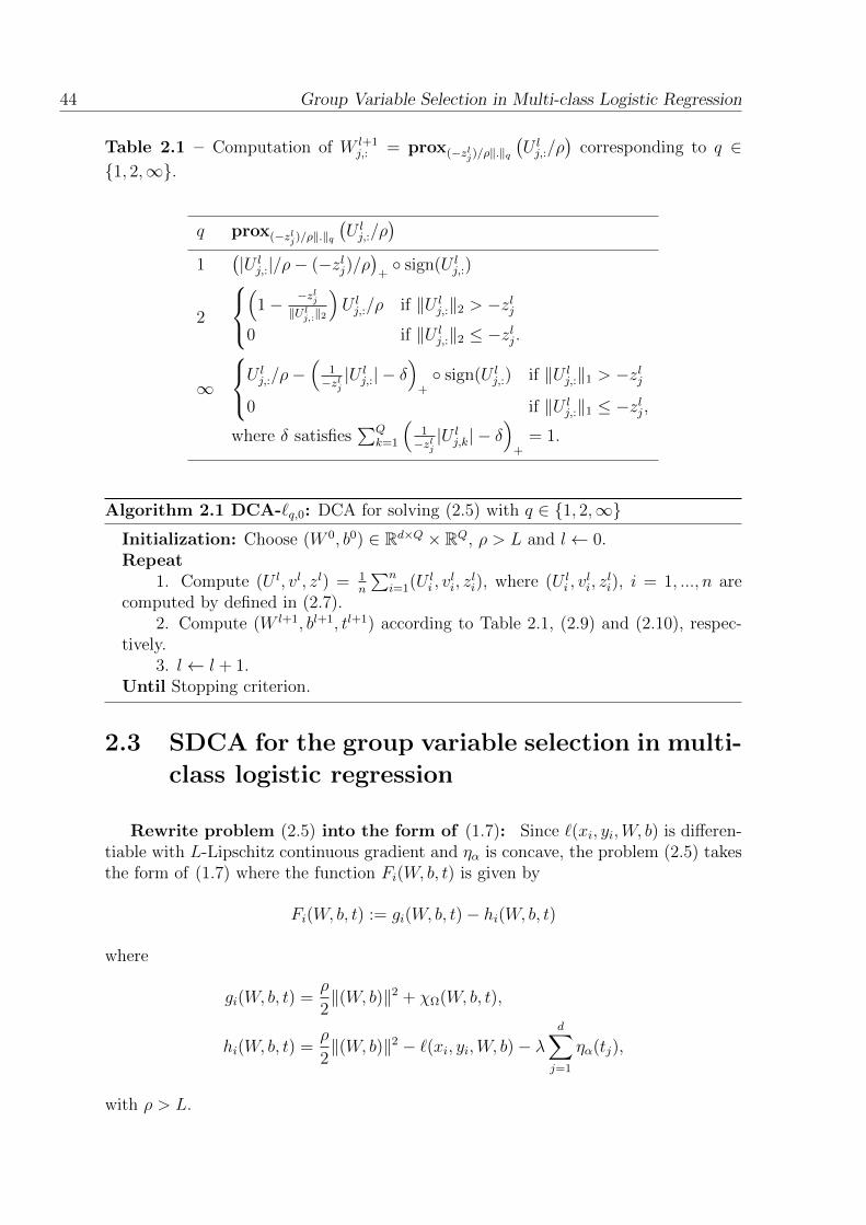
2.1 Computation of W l+1j,: = prox(−zlj)/ρ‖.‖q
(U lj,:/ρ
)corresponding to q ∈
1, 2,∞. . . . . . . . . . . . . . . . . . . . . . . . . . . . . . . . . . . 44
2.2 Comparative results on both synthetic and real datasets.Bold values correspond to best results for each dataset. n, d and Q isthe number of instances, the number of variables and the number ofclasses respectively. . . . . . . . . . . . . . . . . . . . . . . . . . . . . . 51
2.3 Comparative results on group variable selection for multi-class logisticregression. Bold values correspond to best results for each dataset. NAmeans that the algorithm fails to furnish a result. n, d and Q are thenumber of instances, dimensions and classes respectively. Unit of timeis second. . . . . . . . . . . . . . . . . . . . . . . . . . . . . . . . . . . 63
2.4 Comparative results on group variable selection for multi-class logisticregression. Bold values correspond to best results for each dataset. NAmeans that the algorithm fails to furnish a result. n, d and Q are thenumber of instances, dimensions and classes respectively. Unit of timeis second. . . . . . . . . . . . . . . . . . . . . . . . . . . . . . . . . . . 64
3.1 Comparative results on datasets. Bold values correspond to best resultsfor each dataset, n and d are the number of instances and dimensionsrespectively. Unit of time is second. . . . . . . . . . . . . . . . . . . . 71
4.1 Comparative result between algorithms over all datasets. Bold valuescorrespond to best results for each dataset. NA means the algorithmfailed to procedure the result (i.e. Out of Memory). . . . . . . . . . . . 96
4.2 Comparative result between MSSC-JDR and Auto-encoder-based joint-clustering algorithms. Bold values correspond to best results for eachdataset. NA means the algorithm failed to produced a result under 12hours. . . . . . . . . . . . . . . . . . . . . . . . . . . . . . . . . . . . . 100
13

14 List of Tables
4.3 Comparative result between Auto-encoder-based joint-clustering algo-rithms. Bold values correspond to best results for each dataset. NAmeans that the algorithm fails to furnish a result. . . . . . . . . . . . . 108

Abbreviations and Notations
Throughout the dissertation, we use uppercase letters to denote matrices, andlowercase letters for vectors or scalars. Vectors are also regarded as matrices withone column. Some of the abbreviations and notations used in the dissertation aresummarized as follows.
DC Difference of Convex functionsDCA DC Algorithm
R set of real numbersRn set of real column vectors of size n
R the set of extended real numbers, R = R ∪ ±∞‖ · ‖p `p-norm (0 < p <∞), ‖x‖p = (
∑ni=1 |xi|p)1/p, x ∈ Rn
‖ · ‖ Euclidean norm (or `2-norm), ‖x‖ = (∑n
i=1 |xi|2)1/2, x ∈ Rn
‖ · ‖∞ `∞-norm, ‖x‖∞ = maxi=1,...,n |xi|, x ∈ Rn
〈·, ·〉 scalar product, 〈x, y〉 =∑n
i=1 xi.yi, x, y ∈ Rn
χC(·) indicator function of a set C, χC(x) = 0 if x ∈ C, +∞ otherwisecoC convex hull of a set of points CProjC(x) projection of a vector x onto a set Cdom f effective domain of a function f∇f(x) gradient of a function f at x∂f(x) subdifferential of a function f at xWi,: the i-th row of the matrix WW:,i the i-th column of the matrix W the elementwise productIa a-by-a identity matrix1a×b a-by-b matrix of ones|S| cardinality of set S
15

Resume
De nos jours, le Big Data est devenu essentiel et omnipresent dans tous les domaines.Par consequence, il est necessaire de developper des techniques innovantes et efficacespour traiter la croissance rapide du volume des masses de donnees. Nous consideronsles problemes suivants dans le contexte de Big Data : la selection de groupes devariables pour la regression logistique multi-classes, la reduction de dimension par t-SNE ( t-distributed Stochastic Neighbor Embedding en anglais) et l’apprentissageen profondeur pour la classification non-supervisee ( Deep Clustering en anglais).Nous developpons des algorithmes DC (Difference of Convex functions) avances pources problemes, qui sont bases sur la programmation DC et DCA (DC Algorithm) – desoutils puissants pour les problemes d’optimisation non-convexes non-differentiables.
Dans la premiere partie, nous etudions le probleme de la selection de groupes devariables pour la regression logistique multi-classes. Nous resolvons ce probleme en util-isant des DCAs avances – Stochastic DCA et DCA-Like. Plus precisement, StochasticDCA se specialise dans le probleme de la minimisation de la grande somme des fonc-tions DC, et ne necessite qu’un sous-ensemble de fonctions DC a chaque iteration.DCA-Like relaxe la condition de convexite de la deuxieme composante DC en as-surant la convergence. Accelerated DCA-Like integre la technique d’acceleration deNesterov dans DCA-Like pour ameliorer sa performance. Les experiences numeriquessur plusieurs jeux de donnees benchmark de grande taille montrent l’efficacite de tousles algorithmes proposes en termes de temps d’execution et de qualite de la solution.
La deuxieme partie concerne t-SNE, une technique efficace de reduction de di-mension non lineaire. t-SNE est modelise sous forme d’un probleme d’optimisationnon-convexe. Motives par le caractere novateur de DCA-Like et Accelerated DCA-Like, nous developpons ces deux algorithmes pour resoudre le probleme t-SNE. Lasuperiorite de nos algorithmes, appliques a la visualisation de donnees, par rapportaux methodes existantes est illustree via des experiences numeriques realisees sur lesjeux de donnees de tres grande taille.
La troisieme partie est consacree a la classification non-supervisee parl’apprentissage en profondeur. Dans la premiere application, nous proposons deux algo-rithmes bases sur DCA pour combiner t-SNE avec MSSC (Minimum Sum-of-SquaresClustering) par ces deux approches : tandem analysis et joint-clustering. Ladeuxieme application considere le clustering en utilisant l’auto-encodeur. Nous avonspropose une extension d’une classe d’algorithmes de joint-clustering pour resoudre le
17

18 Resume
probleme de mise a l’echelle de donnees ( scaling problem en anglais), et appliquepour un cas specifique de joint-clustering avec MSSC. Les resultats numeriques surplusieurs jeux de donnees benchmark montre l’efficacite de notre algorithme compareaux methodes existantes.
Resume 19
Abstract
Big Data has become gradually essential and ubiquitous in all aspects nowadays.Therefore, there is an urge to develop innovative and efficient techniques to deal withthe rapid growth in the volume of data. This dissertation considers the following prob-lems in Big Data: group variable selection in multi-class logistic regression, dimensionreduction by t-SNE (t-distributed Stochastic Neighbor Embedding), and deep clus-tering. We develop advanced DCAs (Difference of Convex functions Algorithms) forthese problems, which are based on DC Programming and DCA – the powerful toolsfor non-smooth non-convex optimization problems.
Firstly, we consider the problem of group variable selection in multi-class logisticregression. We tackle this problem by using recently advanced DCAs – StochasticDCA and DCA-Like. Specifically, Stochastic DCA specializes in the large sum ofDC functions minimization problem, which only requires a subset of DC functionsat each iteration. DCA-Like relaxes the convexity condition of the second DC com-ponent while guaranteeing the convergence. Accelerated DCA-Like incorporates theNesterov’s acceleration technique into DCA-Like to improve its performance. The nu-merical experiments in benchmark high-dimensional datasets show the effectiveness ofproposed algorithms in terms of running time and solution quality.
The second part studies the t-SNE problem, an effective non-linear dimensionalreduction technique. Motivated by the novelty of DCA-Like and Accelerated DCA-Like, we develop two algorithms for the t-SNE problem. The superiority of proposedalgorithms in comparison with existing methods is illustrated through numerical ex-periments for visualization application.
Finally, the third part considers the problem of deep clustering. In the first appli-cation, we propose two algorithms based on DCA to combine t-SNE with MSSC (Min-imum Sum-of-Squares Clustering) by following two approaches: “tandem analysis”and joint-clustering. The second application considers clustering with auto-encoder(a well-known type of neural network). We propose an extension to a class of joint-clustering algorithms to overcome the scaling problem and applied for a specific caseof joint-clustering with MSSC. Numerical experiments on several real-world datasetsshow the effectiveness of our methods in rapidity and clustering quality, compared tothe state-of-the-art methods.


Introduction generale
Cadre general et motivations
De nos jours, le Big Data est devenu essentiel et omnipresent dans tous les do-maines. Dans la nouvelle ere de l’Internet ou les donnees peuvent etre facilementcollectees (comme les documents, les textes et les videos de l’Internet, les donneessensorielles obtenues a partir de machines), les donnees obtenues ont souvent de nom-breuses variables (c’est-a-dire des donnees de grande dimension) qui posent de nom-breuses difficultes aux techniques classiques d’apprentissage automatique. L’une desfacons les plus naturelles et les plus populaires de traiter les donnees de grande di-mension est d’utiliser des methodes de reduction dimensionnelle. Dans cette these,nous sommes interesses par le developpement de techniques innovantes et efficaces,bien adaptees au Big Data en utilisant des techniques de reduction dimensionnelle :selection de groupes de variables et reduction non lineaire de la dimension.
La selection des variables est une approche simple mais efficace, qui a ete bienetudiee dans la litterature. Cependant, les travaux existants montrent qu’il y a unchevauchement dans les variables selectionnees. De plus, dans de nombreuses ap-plications, nous pouvons avoir des connaissances prealables sur des groupes de vari-ables, il est donc scientifiquement significatif d’incorporer la selection des variables degroupe dans les modeles. La selection de groupes de variables basee sur la normezero-mixte (“mixed-norm”-`q,0 en anglais) est une facon naturelle de modeliser ceprobleme. Cependant, cette derniere n’est pas souvent utilisee en raison de la non-convexite de la `0-norme. Dans ce travail, nous considerons une application de la`q,0-norme pour les donnees de grande dimension en apprentissage automatique. Ladifficulte mentionnee est surmontee en utilisant une fonction DC pour approximerla `0-norme, et le probleme resultant est aussi un probleme d’optimisation DC. Uneautre facon preferee de representer des donnees de grande dimension est d’utiliserdes methodes de reduction non lineaire de la dimension. Cependant, la plupart desproblemes d’optimisation issus de cette direction sont non convexes. Motives par lesucces de la programmation DC et DCA pour plusieurs problemes de reduction nonlineaires de la dimension, tels que la carte auto-organisatrice (“Self-Organizing Map”en anglais) et le positionnement multidimensionnel (“Multidimensional Scaling” enanglais), nous choisissons volontairement la programmation DC et DCA comme labase de methodologie dans cette these.
21

22 Introduction generale
Sur le plan algorithmique, la these a propose une approche unifiee, fondee surla nouvelle generation de la programmation DC et DCA. La programmation DC etDCA (voir [62]) sonts des outils puissants d’optimisation non convexe qui connais-sent un grand succes, au cours de trois dernieres decennies, dans la modelisation etla resolution de nombreux problemes d’application dans divers domaines de sciencesappliquees, en particulier en apprentissage automatique et fouille de donnees (MLDM– “Machine Learning and Data Mining” en anglais) (voir par example [18, 42, 45,47, 48, 49, 55, 56, 57, 58, 59, 60, 63, 64, 66, 67, 71, 84, 85, 86, 87, 125, 111, 50, 52]et la liste des references dans [4]). Recemment, la croissance rapide du Big Data aprovoque plusieurs nouveaux challenges d’optimisation, d’ou une nouvelle generationde DCA voit le jour pour leur confronter d’une facon efficace. Cette these est dedieeau developpement de nouveaux algorithmes bases sur cette nouvelle generation deDCA. De nombreuses experimentations numeriques sur differents types de donneesdans divers domaines realisees dans cette these ont prouve l’efficacite, la scalabilite, larapidite des algorithmes proposes et leur superiorite par rapport aux methodes stan-dards.
La programmation DC et DCA considerent le probleme DC de la forme
α = inff(x) = g(x)− h(x) : x ∈ Rn (Pdc)
ou g et h sont des fonctions convexes definies sur Rn et a valeurs dans R ∪ +∞,semi-continues inferieurement et propres. La fonction f est appelee fonction DC avecles composantes DC g et h, et g−h est une decomposition DC de f . DCA est base surla dualite DC et des conditions d’optimalite locale. La construction de DCA impliqueles composantes DC g et h et non la fonction DC f elle-meme. Chaque fonctionDC admet une infinite des decompositions DC qui influencent considerablement surla qualite (la rapidite, l’efficacite, la globalite de la solution obtenue . . . ) de DCA.Ainsi, au point de vue algorithmique, la recherche d’une “bonne” decomposition DCet d’un “bon” point initial est tres importante dans le developpement de DCA pourla resolution d’un programme DC.
L’utilisation de la programmation DC et DCA dans cette these est justifiee par demultiple arguments [97]:
— La programmation DC et DCA fournissent un cadre tres riche pour lesproblemes MLDM: MLDM constituent une mine des programmes DC dont laresolution appropriee devrait recourir a la programmation DC et DCA. En ef-fet la liste indicative (non exhaustive) des references dans [4] temoigne de lavitalite, la puissance et la percee de cette approche dans la communaute deMLDM.
— DCA est une philosophie plutot qu’un algorithme. Pour chaque probleme, nouspouvons concevoir une famille d’algorithmes bases sur DCA. La flexibilite deDCA sur le choix des decomposition DC peut offrir des schemas DCA plusperformants que des methodes standards.
— L’analyse convexe fournit des outils puissants pour prouver la convergencede DCA dans un cadre general. Ainsi tous les algorithmes bases sur DCAbeneficient (au moins) des proprietes de convergence generales du schema DCAgenerique qui ont ete demontrees.

Introduction generale 23
— DCA est une methode efficace, rapide et scalable pour la programmation nonconvexe. A notre connaissance, DCA est l’un des rares algorithmes de la pro-grammation non convexe, non differentiable qui peut resoudre des programmesDC de tres grande dimension.
Il est important de noter qu’avec les techniques de reformulation en programmationDC et les decompositions DC appropriees, on peut retrouver la plupart des algorithmesexistants en programmation convexe/non convexe comme cas particuliers de DCA. Enparticulier, pour la communaute d’apprentissage automatique et fouille de donnees,les methodes tres connus comme Expectation–Maximisation (EM) [23], Succesive Lin-ear Approximation (SLA) [10], ConCave–Convex Procedure (CCCP) [126], IterativeShrinkage–Thresholding Algorithms (ISTA) [15] sont des versions speciales de DCA.
Nos contributions
L’objectif principal de cette these est de developper de nouveaux modeles etmethodes d’apprentissage automatique dans le Big Data, en particulier pour les troisclasses de problemes suivantes : la selection de groupes de variables pour la regressionlogistique multi-classes, la reduction de dimension par t-SNE, et l’apprentissage enprofondeur pour la classification non-supervisee. Les principales realisations de cettethese seront decrites en detail ci-dessous.
La premier partie concerne le probleme de la selection de groupes de variables enregression logistique multi-classe. Dans la litterature, la norme `q,0 a ete developpeepour formuler le probleme de la selection de groupes de variables. Cependant, leprobleme qui en resulte est difficile a cause de la non-convexite du `q,0. Nous etudionsle DCA pour ce probleme par deux approches. La premiere approche considere leStochastic DCA. Ce dernier est specifiquement developpe pour le probleme “large sumof DC functions”. L’avantage principal de cette methode par rapport a la methodeDCA standard est qu’elle ne necessite que le calcul du sous-gradient d’un sous-ensemblede la deuxieme composante DC. Dans la deuxieme approche, nous avons considereDCA-Like et Accelerated DCA-Like. Contrairement a DCA standard, le DCA-Likerelaxe la condition de convexite de la deuxieme composante DC tout en assurantla convergence. DCA-Like accelere integre la technique d’acceleration de Nesterovdans DCA-Like pour ameliorer sa performance tout en beneficiant de proprietes deconvergence similaires a celles de DCA-Like. Les experiences numeriques sur les jeuxde donnees de tres grande taille (synthetiques et reelles) montrent que nos methodessont efficaces en terms de qualite et de temps de calcul.
La deuxieme partie etudie le probleme de la reduction dimensionnelle par t-SNE.Cette derniere est une methode populaire, en particulier pour la visualisation. Elle a eteutilisee dans de nombreuses applications telles que la bioinformatique, la recherche surle cancer, la visualisation de “features” dans les reseaux neuronaux, etc. Cependant, ils’agit d’un probleme difficile d’optimisation non convexe. Nous etudions le DCA pource probleme et nous proposons deux algorithmes efficaces bases sur deux DCA avances– DCA-like et Accelerated DCA-Like. Nous montrons egalement que la minimisationde la majorisation [123], le meilleur algorithme pour t-SNE, n’est rien d’autre que DCA-Like applique au t-SNE. Nous effectuons soigneusement les experiences numeriques et
24 Introduction generale
fournissons une comparaison des algorithmes proposes sur plusieurs jeux de donneesbenchmarks pour l’application de visualisation.
La troisieme partie concerne l’apprentissage en profondeur (“Deep Clustering” enanglais) pour la classification non-supervisee (clustering) pour les donnees de grandedimension. Dans la litterature, les problemes “deep clustering” sont souvent abordesen utilisant des techniques de reduction dimensionnelle, qui ont donne les meilleursresultats dans de nombreuses applications de clustering, en particulier pour les donneescomplexes de grande dimension comme les images et les documents. Nous consideronsdeux directions basees sur deux methodes de reduction de la dimension – t-SNE etauto-encodeur. Dans la premiere direction, le t-SNE est considere par deux approches :“tandem analysis” et joint-clustering. Nous avons developpe deux algorithmes basessur la programmation DC et DCA. Le premier algorithme, appele MSSC-2S, suitl’approche de “tandem analysis”, qui utilise t-SNE pour la reduction de la dimen-sionnalite avant le clustering. Puisque chaque etape du MSSC-2S est effectuee par unDCA bien adapte aux jeux de donnees de grande dimension, le MSSC-2S est applica-ble aux contextes de grande dimension. La deuxieme direction considere le problemede l’optimisation non-convexe pour les taches de clustering et de reduction de la di-mension. Nous developpons une methode efficace, MSSC-JDR, par la programmationDC et DCA. Nous effectuons des experiences extensives pour des jeux de donneesde grande dimension et a grande dimension avec plusieurs methodes recentes pourdemontrer l’efficacite de nos algorithmes. Dans la deuxieme direction, nous consideronsl’auto-encodeur sur l’approche de joint-clustering. Nous montrons d’abord qu’il existeune classe d’algorithmes qui sont affectes par le probleme d’echelle dans l’espace la-tent. Ensuite, nous proposons des extensions en utilisant deux fonctions de distanced’invariance d’echelle. En tant qu’application, les extensions proposees sont appliqueesau probleme de joint-clustering avec MSSC (Minimum Sum-of-Square Clustering). Lesexperimentations numeriques sont effectuees sur des ensembles de donnees de grandedimension demontrent la qualite des extensions proposees par rapport aux methodesexistantes.
Organisation de la These
La these est composee de cinq chapitres. Le premier chapitre decrit brievementles concepts fondamentaux et les principaux resultats de l’analyse convexe, la pro-grammation DC et DCA, et ses versions avancees, ce qui fournit la base theoriqueet algorithmique pour les autres chapitres. Chacun des trois chapitres suivants estconsacre a la presentation d’une classe de problemes abordee ci-dessus. Le chapitre2 concerne le probleme de la selection de groupes de variables pour la regression lo-gistique multi-classe. Ensuite, le chapitre 3 considere au probleme du t-SNE. Dans lechapitre 4, nous abordons les problemes clustering en d’apprentissage en profondeur.La conclusion et les perspectives de nos travaux sont donnees au chapitre 5.

Chapter 1
Methodology
This chapter summarizes some basic concepts and results that will be the ground-work of the dissertation.
1.1 DC programming and DCA
DC programming and DCA, which constitute the backbone of nonconvex program-ming and global optimization, were introduced by Pham Dinh Tao in their preliminaryform in 1985 [88]. Important developments and improvements on both theoretical andcomputational aspects have been completed since 1994 throughout the joint works ofLe Thi Hoai An and Pham Dinh Tao. The readers are referred to the seminal paper [62]for the thirty years of developments of DCA.
In this section, we present some basic properties of convex analysis and DC opti-mization and DC Algorithm that computational methods of this thesis are based on.The materials of this section are extracted from [44, 85, 60].
1.1.1 Fundamental convex analysis
First, let us recall briefly some notions and results in convex analysis related tothe dissertation (refer to the references [9, 85, 93] for more details). Let denote X theEuclidean space Rn.
A subset C of X is said to be convex if (1− λ)x+ λy ∈ C whenever x, y ∈ C andλ ∈ [0, 1].
Let f be a function whose values are in R and whose domain is a subset S of X.The set
(x, t) : x ∈ S, t ∈ R, f(x) ≤ tis called the epigraph of f and is denoted by epif .
25
-
26 Preliminary
We define f to be a convex function on S if epif is convex set in X × R. This isequivalent to that S is convex and
f((1− λ)x+ λy) ≤ (1− λ)f(x) + λf(y), ∀x, y ∈ S, ∀λ ∈ [0, 1].
The function f is strictly convex if the inequality above holds strictly whenever x andy are distinct in S and 0 < λ < 1.
The effective domain of a convex function f on S, denoted by domf , is the projec-tion on X of the epigraph of f
domf = x ∈ X : ∃t ∈ R, (x, t) ∈ epif = x ∈ X : f(x) < +∞
and obviously, it is convex.
The convex function f is called proper if domf 6= ∅ and f(x) > −∞ for all x ∈ S.
The function f is said to be lower semi-continuous at a point x of S if
f(x) ≤ lim infy→x
f(y).
Denote by Γ0(X) the set of all proper lower semi-continuous convex functions onX.
Let ρ be a nonnegative number and C be a convex subset of X. One says that afunction θ : C → R ∪ +∞ is ρ–convex if
θ[λx+ (1− λ)y] ≤ λθ(x) + (1− λ)θ(y)− λ(1− λ)
2ρ‖x− y‖2
for all x, y ∈ C and λ ∈ (0, 1). It amounts to say that θ − (ρ/2)‖ · ‖2 is convex on C.The modulus of strong convexity of θ on C, denoted by ρ(θ, C) or ρ(θ) if C = X, isgiven by
ρ(θ, C) = supρ ≥ 0 : θ − (ρ/2)‖ · ‖2 is convex on C.
One says that θ is strongly convex on C if ρ(θ, C) > 0.
A vector y is said to be a subgradient of a convex function f at a point x0 if
f(x) ≥ f(x0) + 〈x− x0, y〉, ∀x ∈ X.
The set of all subgradients of f at x0 is called the subdifferential of f at x0 and isdenoted by ∂f(x0). If ∂f(x) is not empty, f is said to be subdifferentiable at x.
For ε > 0, a vector y is said to be an ε–subgradient of a convex function f at apoint x0 if
f(x) ≥ (f(x0)− ε) + 〈x− x0, y〉, ∀x ∈ X.
The set of all ε–subgradients of f at x0 is called the ε–subdifferential of f at x0 and isdenoted by ∂εf(x0).
Preliminary 27
For ε ≥ 0, a point xε is called an ε-solution of the problem inff(x) : x ∈ Rd if
f(xε) ≤ f(x) + ε ∀x ∈ Rd.
Let us describe two basic notations as follows.
dom ∂f = x ∈ X : ∂f(x) 6= ∅ and range ∂f(x) = ∪∂f(x) : x ∈ dom ∂f.
Proposition 1.1. Let f be a proper convex function. Then
1. ∂εf(x) is a closed convex set, for any x ∈ X and ε ≥ 0.
2. ri(domf) ⊂ dom ∂f ⊂ domfwhere ri(domf) stands for the relative interior of domf .
3. If f has a unique subgradient at x, then f is differentiable at x, and ∂f(x) =∇f(x).
4. x0 ∈ argminf(x) : x ∈ X if and only if 0 ∈ ∂f(x0).
Conjugates of convex functions
The conjugate of a function f : X → R is the function f ∗ : X → R, defined by
f ∗(y) = supx∈X〈x, y〉 − f(x).
Proposition 1.2. Let f ∈ Γ0(X). Then we have
1. f ∗ ∈ Γ0(X) and f ∗∗ = f .
2. f(x) + f ∗(y) ≥ 〈x, y〉, for any x, y ∈ X.Equality holds if and only if y ∈ ∂f(x)⇔ x ∈ ∂f ∗(y).
3. y ∈ ∂εf(x)⇐⇒ x ∈ ∂εf ∗(y)⇐⇒ f(x) + f ∗(y) ≤ 〈x, y〉+ ε, for all ε > 0.
1.1.2 DC optimization
DC program
In the sequel, we use the convention +∞− (+∞) = +∞.
For g, h ∈ Γ0(X), a standard DC program is of the form
(P ) α = inff(x) = g(x)− h(x) : x ∈ X
and its dual counterpart
(D) α∗ = infh∗(y)− g∗(y) : y ∈ X.
There is a perfect symmetry between primal and dual programs (P ) and (D): thedual program to (D) is exactly (P ), moreover, α = α∗.

28 Preliminary
Remark 1.1. Let C be a nonempty closed convex set. Then, the constrained problem
inff(x) = g(x)− h(x) : x ∈ C
can be transformed into an unconstrained DC program by using the indicator functionχC, i.e.,
inff(x) = φ(x)− h(x) : x ∈ X
where φ := g + χC belongs to Γ0(X).
We will always keep the following assumption that is deduced from the finitenessof α
dom g ⊂ domh and domh∗ ⊂ dom g∗. (1.1)
Optimality conditions for DC optimization
A point x∗ is said to be a local minimizer of g − h if x∗ ∈ dom g ∩ domh (so,(g − h)(x∗) is finite) and there is a neighborhood U of x∗ such that
g(x)− h(x) ≥ g(x∗)− h(x∗), ∀x ∈ U. (1.2)
A point x∗ is said to be a critical point of g−h if it verifies the generalized Kuhn–Tuckercondition
∂g(x∗) ∩ ∂h(x∗) 6= ∅. (1.3)
Let P and D denote the solution sets of problems (P ) and (D) respectively, and let
P` = x∗ ∈ X : ∂h(x∗) ⊂ ∂g(x∗), D` = y∗ ∈ X : ∂g∗(y∗) ⊂ ∂h∗(y∗).
In the following, we present some fundamental results on DC programming [85].
Theorem 1.1. i) Global optimality condition: x ∈ P if and only if
∂εh(x) ⊂ ∂εg(x), ∀ε > 0.
ii) Transportation of global minimizers: ∪∂h(x) : x ∈ P ⊂ D ⊂ domh∗.The first inclusion becomes equality if g∗ is subdifferentiable in D. In this case,D ⊂ (dom ∂g∗ ∩ dom ∂h∗).
iii) Necessary local optimality: if x∗ is a local minimizer of g − h, then x∗ ∈ P`.iv) Sufficient local optimality: Let x∗ be a critical point of g−h and y∗ ∈ ∂g(x∗)∩
∂h(x∗). Let U be a neighborhood of x∗ such that (U ∩ dom g) ⊂ dom ∂h. If forany x ∈ U ∩dom g, there is y ∈ ∂h(x) such that h∗(y)−g∗(y) ≥ h∗(y∗)−g∗(y∗),then x∗ is a local minimizer of g − h. More precisely,
g(x)− h(x) ≥ g(x∗)− h(x∗), ∀x ∈ U ∩ dom g.
Preliminary 29
v) Transportation of local minimizers: Let x∗ ∈ dom ∂h be a local minimizer ofg − h. Let y∗ ∈ ∂h(x∗) and a neighborhood U of x∗ such that g(x) − h(x) ≥g(x∗)− h(x∗), ∀x ∈ U ∩ dom g. If
y∗ ∈ int(dom g∗) and ∂g∗(y∗) ⊂ U
then y∗ is a local minimizer of h∗ − g∗.
Remark 1.2. a) By the symmetry of the DC duality, these results have their cor-responding dual part. For example, if y is a local minimizer of h∗ − g∗, theny ∈ D`.
b) The properties ii), v) and their dual parts indicate that there is no gap betweenthe problems (P ) and (D). They show that globally/locally solving the primalproblem (P ) implies globally/locally solving the dual problem (D) and vice–versa.Thus, it is useful if one of them is easier to solve than the other.
c) The necessary local optimality condition ∂h∗(x∗) ⊂ ∂g∗(x∗) is also sufficient formany important classes programs, for example [60], if h is polyhedral convex,or when f is locally convex at x∗, i.e. there exists a convex neighborhood U ofx∗ such that f is finite and convex on U . We know that a polyhedral convexfunction is almost everywhere differentiable, that is to say, it is differentiableeverywhere except on a set of measure zero. Thus, if h is a polyhedral convexfunction, then a critical point of g − h is almost always a local solution to (P ).
d) If f is actually convex on X, we call (P) a “false” DC program. In addition, ifri(dom g)∩ ri(domh) 6= ∅ and x0 ∈ dom g such that g is continuous at x0, then0 ∈ ∂f(x0) ⇔ ∂h(x0) ⊂ ∂g(x0) [60]. Thus, in this case, the local optimalityis also sufficient for the global optimality. Consequently, if in addition h isdifferentiable, a critical point is also a global solution.
1.1.3 DC Algorithm (DCA)
The DCA consists in the construction of the two sequences xk and yk (can-didates for being primal and dual solutions, respectively) which are easy to calculateand satisfy the following properties:
i) The sequences (g − h)(xk) and (h∗ − g∗)(yk) are decreasing.
ii) Their corresponding limits x∞ and y∞ either satisfy the local optimality condi-tion (x∞, y∞) ∈ P`×D` or are critical points of g−h and h∗− g∗, respectively.
From a given initial point x0 ∈ dom g, the DCA generates these sequences by thescheme
yk ∈ ∂h(xk) = arg minh∗(y)− 〈y, xk〉 : y ∈ X, (1.4a)
xk+1 ∈ ∂g∗(yk) = arg ming(x)− 〈x, yk〉 : x ∈ X. (1.4b)
The interpretation of the above scheme is simple. At iteration k of DCA, onereplaces the second component h in the primal DC program by its affine minorant
hk(x) = h(xk) + 〈x− xk, yk〉, (1.5)
30 Preliminary
where yk ∈ ∂h(xk). Then the original DC program is reduced to the convex program
(Pk) αk = inffk(x) := g(x)− hk(x) : x ∈ X
that is equivalent to (1.4b). It is easy to see that fk is a majorant of f which is exactat xk i.e. fk(x
k) = f(xk). Similarly, by replacing g∗ with its affine minorant
g∗k(y) = g∗(yk−1) + 〈y − yk−1, xk〉 (1.6)
where xk ∈ ∂g∗(yk−1), it leads to the convex program
(Dk) infh∗(y)− g∗k(y) : y ∈ X
whose solution set is ∂h(xk).
Well definiteness of DCA
DCA is well defined if one can construct two sequences xk and yk as describedabove from an arbitrary initial point. The following lemma is the necessary and suffi-cient condition for this property.
Lemma 1.1 ([85]). The sequences xk and yk in DCA are well defined if and onlyif
dom ∂g ⊂ dom ∂h and dom ∂h∗ ⊂ dom ∂g∗.
Since for ϕ ∈ Γ0(X) one has ri(domϕ) ⊂ dom ∂ϕ ⊂ domϕ (Proposition 1.1).Moreover, under the assumptions dom g ⊂ domh, domh∗ ⊂ dom g∗, one can say thatDCA in general is well defined.
Convergence properties of DCA
Complete convergence of DCA is given in the following results [85].
Theorem 1.2. Suppose that the sequences xk and yk are generated by DCA. Thenwe have
i) The sequences g(xk)− h(xk) and h∗(yk)− g∗(yk) are decreasing and
• g(xk+1)−h(xk+1) = g(xk)−h(xk) if and only if xk, xk+1 ⊂ ∂g∗(yk)∩∂h∗(yk)and [ρ(h) + ρ(g)]‖xk+1 − xk‖ = 0.
• h∗(yk+1) − g∗(yk+1) = h∗(yk) − g∗(yk) if and only if yk, yk+1 ⊂ ∂g(xk) ∩∂h(xk) and [ρ(h∗) + ρ(g∗)]‖yk+1 − yk‖ = 0.
DCA terminates at the kth iteration if either of the above equalities holds.
ii) If ρ(h) + ρ(g) > 0 (resp. ρ(h∗) + ρ(g∗) > 0), then the sequence ‖xk+1 − xk‖2(resp. ‖yk+1 − yk‖2) converges.
iii) If the optimal value α is finite and the sequences xk and yk are bounded,then every limit point x∞ (resp. y∞) of the sequence xk (resp. yk) is acritical point of g − h (resp. h∗ − g∗).
Preliminary 31
iv) DCA has a linear convergence for general DC program.
v) In polyhedral DC programs, the sequences xk and yk contain finitely manyelements and DCA has a finite convergence.
vi) If DCA converges to a point x∗ that admits a convex neighborhood in which theobjective function f is finite and convex (i.e. the function f is locally convex atx∗) and if the second DC component h is differentiable at x∗, then x∗ is a localminimizer to the problem (P ).
Remark 1.3. a) Finding yk, xk+1 based on the scheme 1.4 amounts to solving theproblems (Dk) and (Pk). Thus, DCA works by reducing a DC program to asequence of convex programs which can be solved efficiently.
b) In practice, the calculation of the subgradient of the function h at a point x isusually easy if we know its explicit expression. But, the explicit expression ofthe conjugate of a given function g is unknown, so calculating xk+1 is done bysolving the convex problem (Pk). For the large-scale setting, the solutions tothe problem (Pk) should be either in an explicit form or achieved by efficientalgorithms with inexpensive computations.
c) DCA’s distinctive feature relies upon the fact that DCA deals with the convexDC components g and h but not with the DC function f itself. Moreover,a DC function f has infinitely many DC decompositions which have crucialimplications for the qualities (e.g. convergence speed, robustness, efficiency,globality of computed solutions) of DCA. For a given DC program, the choiceof optimal DC decompositions is still open. Of course, this depends strongly onthe very specific structure of the problem being considered.
d) Similarly to the effect of DC decompositions on DCA, searching the good initialpoints for DCA is also an open question to be studied.
1.2 Stochastic DCA 1
The large sum of DC functions minimization problem takes the form
minx∈Rd
F (x) :=
1
n
n∑i=1
Fi(x)
, (1.7)
where Fi are DC functions, i.e., Fi(x) = gi(x) − hi(x) with gi and hi being lowersemi-continuous proper convex functions, and n is a very large integer number. Theproblem of minimizing F under a convex set Ω is also of the type (1.7), as the convexconstraint x ∈ Ω can be incorporated into the objective function F via the indicatorfunction χΩ on Ω defined by χΩ = 0 if x ∈ Ω, +∞ otherwise.
A natural DC formulation of the problem (1.7) is
minF (x) = G(x)−H(x) : x ∈ Rd
, (1.8)
1. The material of this section is from the following work: H.A. Le Thi, H.M. Le, D.N. Phan,B. Tran. Stochastic DCA for minimizing a large sum of DC functions and its application in Multi-class Logistic Regression. Submitted & Available on arvXiv [arXiv:1911.03992].
32 Preliminary
where
G(x) =1
n
n∑i=1
gi(x) and H(x) =1
n
n∑i=1
hi(x).
According to the generic DCA scheme, DCA for solving the problem (1.8) consistsof computing, at each iteration l, a subgradient vl ∈ ∂H(xl) and solving the convexsubproblem of the form
minG(x)− 〈vl, x〉 : x ∈ Rd
. (1.9)
As H =∑n
i=1 hi, the computation of subgradients of H requires the one of all functionshi. This may be expensive when n is very large. The main idea of SDCA is to update,at each iteration, the minorant of only some randomly chosen hi while keeping theminorant of the other hi. Hence, only the computation of such randomly chosen hi isrequired.
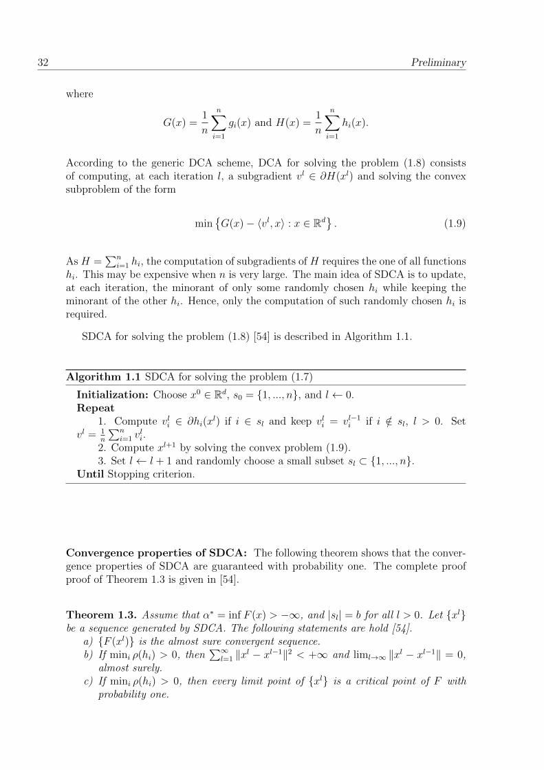
SDCA for solving the problem (1.8) [54] is described in Algorithm 1.1.
Algorithm 1.1 SDCA for solving the problem (1.7)
Initialization: Choose x0 ∈ Rd, s0 = 1, ..., n, and l← 0.Repeat
1. Compute vli ∈ ∂hi(xl) if i ∈ sl and keep vli = vl−1
i if i /∈ sl, l > 0. Setvl = 1
n
∑ni=1 v
li.
2. Compute xl+1 by solving the convex problem (1.9).3. Set l← l + 1 and randomly choose a small subset sl ⊂ 1, ..., n.
Until Stopping criterion.
Convergence properties of SDCA: The following theorem shows that the conver-gence properties of SDCA are guaranteed with probability one. The complete proofproof of Theorem 1.3 is given in [54].
Theorem 1.3. Assume that α∗ = inf F (x) > −∞, and |sl| = b for all l > 0. Let xlbe a sequence generated by SDCA. The following statements are hold [54].
a) F (xl) is the almost sure convergent sequence.b) If mini ρ(hi) > 0, then
∑∞l=1 ‖xl − xl−1‖2 < +∞ and liml→∞ ‖xl − xl−1‖ = 0,
almost surely.c) If mini ρ(hi) > 0, then every limit point of xl is a critical point of F with
probability one.
Preliminary 33
1.3 DCA-Like and Accelerated DCA-Like 1
First, let us considers the sum of a nonconvex differentiable function and compositefunctions minimization problem, which takes the form
minx∈X
F (x) := f(x) +
m∑i=1
hi(gi(xi))
, (1.10)
where f : Rn → R is a nonconvex differentiable function with L-Lipschitz continuousgradient; gi : Rni → R (i = 1 . . . n) are continuous convex functions (possibly nons-mooth) with
∑mi=1 ni = n; real functions hi are concave increasing and ∂(−hi)(t) ⊂ R−
if t ≥ gi(xi) and X is a closed convex subset of Rn.
1.3.1 DCA for the problem (1.10)
This section outlines the DCA based algorithm to solve the sum of nonconvexand composite functions minimization problem (1.10) in [53]. The problem (1.10) isformulated as follows:
min(x,z)
ϕ(x, z) := χΩ(x, z) + f(x) +
m∑i=1
hi(zi)
, (1.11)
where Ω = (x, z) : x ∈ X, gi(xi) ≤ zi, i = 1, ...,m and χΩ is the indicator functionof Ω. Let g(x) be the function defined by g(x) = (g1(x1), ..., gm(xm)). The problems(1.10) and (1.11) are equivalent in the following sense.
Proposition 1.3. [53] A point x∗ ∈ X is a global (resp. local) solution to the problem(1.10) if and only if (x∗, g(x∗)) is a global (resp. local) solution to the problem (1.11).
Since the problems (1.10) and (1.11) are equivalent, in the remaining of the sec-tion 1.3, we consider the problem (1.11) instead of (1.10). Furthermore, the problem(1.11) can be rewritten as
min(x,z)ϕ(x, z) = Gµ(x, z)−Hµ(x, z) , (1.12)
where Gµ(x, z) := µ2‖x‖2 + χΩ(x, z) and Hµ(x, z) := µ
2‖x‖2 − f(x)−
∑mi=1 hi(zi) with
µ > 0. It is easy to see that Gµ(x, z) is convex since Ω is a convex set. On the otherhand, ∇f is Lipschitz continuous with a constant L, hence µ
2‖x‖2 − f(x) is convex
if µ ≥ L. Consequently, Hµ(x, z) is convex, and (1.11) is a standard DC programwith µ ≥ L. Thus DCA can be investigated to solve the problem (1.11). At each
1. The material of this section is from the following work: H.A. Le Thi, H.M. Le, D.N. Phan,B. Tran. Novel DCA Based Algorithms for Minimizing the Sum of a Nonconvex Function andComposite Functions with Applications in Machine learning. Submitted & Available on arvXiv[arXiv:1806.09620].

34 Preliminary
iteration k, DCA approximates the second DC component Hµ by its affine minorant
H(xk,zk)µ (x, z) = Hµ(xk, zk)+〈(x, z)−(xk, zk), (yk, ξk)〉 with (yk, ξk) ∈ ∂Hµ(xk, zk) and
computes (xk+1, zk+1) by solving the following convex problem
minϕkµ(x, z) := Gµ(x, z)−Hk
µ(x, z). (1.13)
Note that ϕkµ is a majorant of ϕ. The convex sub-problem (1.13) can be rewritten asfollows
min(x,z)∈Ω
µ
2‖x‖2 − 〈yk,x〉+
m∑i=1
(−ξki )zi
, (1.14)
where ξki ∈ ∂(−hi)(zki ).
Lemma 1.2 [53] shows that an optimal solution of (1.14) can be obtained by solvinga strongly convex problem without the variables z.
Lemma 1.2. [53] If xk+1 is an optimal solution of the following strongly convexproblem
minx∈Xµ
2‖x‖2 − 〈yk,x〉+
m∑i=1
(−ξki )gi(xi), (1.15)
then (xk+1, zk+1), where zk+1 = g(xk+1), is an optimal solution of (1.14).
Finally, DCA for solving (1.11) is described in Algorithm 1.2.
Algorithm 1.2 DCA for solving (1.11)
Initialize:Choose x0, µ ≥ L, and k ← 0.
repeat1. Compute ξki ∈ ∂(−hi)(zki ) with zki = gi(x
ki ) and yk = µxk −∇f(xk)
2. Compute xk+1 by solving the strongly convex problem (1.15)3. k ← k + 1.
until Stopping criterion
The convergence properties of Algorithm 1.2 are provided in the Theorem 1.4 [53].We recall that a point (x∗, z∗) ∈ Rn×Rm is called a critical point of the problem (1.11)if and only if
[(∇f(x∗), 0m) +NΩ(x∗, z∗)] ∩ [0n × ∂(−h1)(z∗1)× ...× ∂(−hm)(z∗m)] 6= ∅,where 0d denotes the zero vector in Rd, and NΩ(u∗) is the normal cone of Ω at u∗
defined byNΩ(u∗) = v : 〈v,u− u∗〉 ≤ 0,∀u ∈ Ω .
Theorem 1.4. [53] Let xk be the sequence generated by Algorithm 1.2. The fol-lowing statements hold.
i) The sequence ϕ(xk, g(xk)) is decreasing.ii) If α = inf ϕ(x, z) > −∞ then
∑+∞k=0 ‖xk+1 − xk‖2 < +∞, and therefore
limk→+∞ ‖xk+1 − xk‖ = 0.iii) If α = inf ϕ(x, z) > −∞, then any limit point of (xk, g(xk)) is a critical
point of (1.11).
Preliminary 35
1.3.2 DCA-Like for solving the problem (1.11)
This section presents DCA-Like for for solving (1.11) [53]. As we have mentionedabove, the goal of DCA-Like is to avoid bad approximations of the objective functionwith a too large value of µ (c.f. Algorithm 1.2). The main idea of DCA-Like is tokeep the parameter µ as small as possible while finding a convex approximation ofobjecive function. By using a small value of µk, we can get a closer majorant ofthe objective function which could lead to a better solution. DCA-Like relaxes the
key requirement of standard DCA that the minorant H(xk,zk)µ (x, z) = Hµ(xk, zk) +
〈(x, z) − (xk, zk), (yk, ξk)〉 must be a lower bound of the second component Hµ(x, z)on the whole space. More precisely, at each iteration k, we only need to find µk such
that H(xk,zk)µk (x, z) is a lower bound of Hµk(x, z) at xk+1, zk+1, i.e.,
Hµk(xk+1, zk+1) ≥ H(xk,g(xk))
µk(xk+1, zk+1). (1.16)
where (xk+1, zk+1) ∈ arg minϕkµk(x, z).
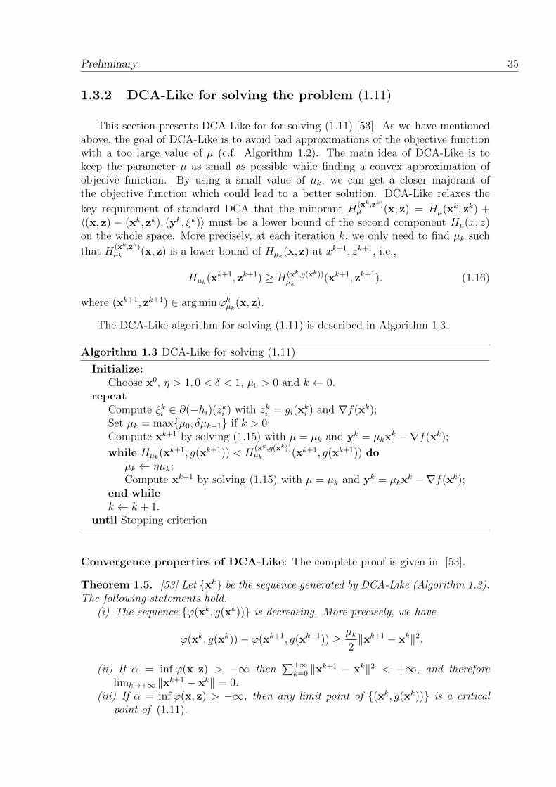
The DCA-Like algorithm for solving (1.11) is described in Algorithm 1.3.
Algorithm 1.3 DCA-Like for solving (1.11)
Initialize:Choose x0, η > 1, 0 < δ < 1, µ0 > 0 and k ← 0.
repeatCompute ξki ∈ ∂(−hi)(zki ) with zki = gi(x
ki ) and ∇f(xk);
Set µk = maxµ0, δµk−1 if k > 0;Compute xk+1 by solving (1.15) with µ = µk and yk = µkx
k −∇f(xk);
while Hµk(xk+1, g(xk+1)) < H
(xk,g(xk))µk (xk+1, g(xk+1)) do
µk ← ηµk;Compute xk+1 by solving (1.15) with µ = µk and yk = µkx
k −∇f(xk);end whilek ← k + 1.
until Stopping criterion
Convergence properties of DCA-Like: The complete proof is given in [53].
Theorem 1.5. [53] Let xk be the sequence generated by DCA-Like (Algorithm 1.3).The following statements hold.
(i) The sequence ϕ(xk, g(xk)) is decreasing. More precisely, we have
ϕ(xk, g(xk))− ϕ(xk+1, g(xk+1)) ≥ µk2‖xk+1 − xk‖2.
(ii) If α = inf ϕ(x, z) > −∞ then∑+∞
k=0 ‖xk+1 − xk‖2 < +∞, and thereforelimk→+∞ ‖xk+1 − xk‖ = 0.
(iii) If α = inf ϕ(x, z) > −∞, then any limit point of (xk, g(xk)) is a criticalpoint of (1.11).
36 Preliminary
Theorem 1.6. [53] Suppose that inf ϕ(x, z) > −∞, and hi is differentiable withlocally Lipschitz derivative. Assume further that ϕ has the KL property at any point(x, z) ∈ dom ∂Lϕ. If xk generated by DCA-Like is bounded, then the whole sequencexk converges to x∗, which (x∗, g(x∗)) is a critical point of (1.11). Moreover, if thefunction ψ appearing in the KL inequality has the form ψ(s) = cs1−θ with θ ∈ [0, 1)and c > 0, then the following statements hold:
(i) If θ = 0, then the sequences xk and ϕ(xk, g(xk)) converge in a finite numberof steps to x∗ and ϕ∗, respectively.
(ii) If θ ∈ (0, 1/2], then the sequences xk and ϕ(xk, g(xk)) converge linearlyto x∗ and ϕ∗, respectively.
(iii) If θ ∈ (1/2, 1), then there exist positive constants δ1, δ2, and N0 such that
‖xk − x∗‖ ≤ δ1k− 1−θ
2θ−1 and ϕ(xk, g(xk))− ϕ∗ ≤ δ2k− 1
2θ−1 for all k ≥ N0.
1.3.3 Accelerated DCA-Like Algorithm for problem (1.11)
According to the DCA-Like scheme, at each iteration, one computes xk+1 fromxk by solving the convex sub-problem (1.15). The idea of ADCA-Like (AcceleratedDCA-Like) [53], in order to accelerate DCA-Like, is to find a point wk which is betterthan xk for the computation of xk+1. In this work, we consider wk as an extrapolatedpoint of the current iterate xk and the previous iterate xk−1:
wk = xk +tk − 1
tk+1
(xk − xk−1
),
where tk+1 =1+√
1+4t2k2
. If wk is better than the last iterate xk, i.e., ϕ(wk, g(wk)) ≤ϕ(xk, g(xk)) then wk will be used instead of xk to compute xk+1. Note that, ADCA-Like does not require any particular property of the sequence tk. ADCA-Like algo-rithm for solving (1.11) is described in Algorithm 1.4.
In Theorem 1.7, we show that any limit point of the sequence generated by ADCA-Like is a critical point of (1.11). The complete proof of the convergence is given in[53].
Theorem 1.7. [53] Let xk be the sequence generated by Algorithm 1.4. The fol-lowing statements hold
(i) The sequence ϕ(xk, g(xk)) is decreasing. More precisely, we have
ϕ(xk, g(xk))− ϕ(xk+1, g(xk+1)) ≥ µk2‖xk+1 − vk‖2.
(ii) If α = inf ϕ(x, z) > −∞ then∑+∞
k=0 ‖xk+1 − vk‖2 < +∞ and thereforelimk→+∞ ‖xk+1 − vk‖ = 0.
(iii) If α = inf ϕ(x, z) > −∞, then any limit point of (xk, g(xk)) is a criticalpoint of (1.11).
Preliminary 37
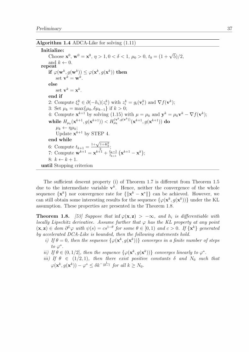
Algorithm 1.4 ADCA-Like for solving (1.11)
Initialize:Choose x0, w0 = x0, η > 1, 0 < δ < 1, µ0 > 0, t0 = (1 +
√5)/2,
and k ← 0.repeat
if ϕ(wk, g(wk)) ≤ ϕ(xk, g(xk)) thenset vk = wk.
elseset vk = xk.
end if2: Compute ξki ∈ ∂(−hi)(zki ) with zki = gi(v
ki ) and ∇f(vk);
3: Set µk = maxµ0, δµk−1 if k > 0;4: Compute xk+1 by solving (1.15) with µ = µk and yk = µkv
k −∇f(vk);
while Hµk(xk+1, g(xk+1)) < H
(vk,g(vk))µk (xk+1, g(xk+1)) do
µk ← ηµk;Update xk+1 by STEP 4.
end while
6: Compute tk+1 =1+√
1+4t2k2
;7: Compute wk+1 = xk+1 + tk−1
tk+1
(xk+1 − xk
);
8: k ← k + 1.until Stopping criterion
The sufficient descent property (i) of Theorem 1.7 is different from Theorem 1.5due to the intermediate variable vk. Hence, neither the convergence of the wholesequence xk nor convergence rate for ‖xk − x∗‖ can be achieved. However, wecan still obtain some interesting results for the sequence ϕ(xk, g(xk)) under the KLassumption. These properties are presented in the Theorem 1.8.
Theorem 1.8. [53] Suppose that inf ϕ(x, z) > −∞, and hi is differentiable withlocally Lipschitz derivative. Assume further that ϕ has the KL property at any point(x, z) ∈ dom ∂Lϕ with ψ(s) = cs1−θ for some θ ∈ [0, 1) and c > 0. If xk generatedby accelerated DCA-Like is bounded, then the following statements hold.
i) If θ = 0, then the sequence ϕ(xk, g(xk)) converges in a finite number of stepsto ϕ∗.
ii) If θ ∈ (0, 1/2], then the sequence ϕ(xk, g(xk)) converges linearly to ϕ∗.iii) If θ ∈ (1/2, 1), then there exist positive constants δ and N0 such that
ϕ(xk, g(xk))− ϕ∗ ≤ δk−1
2θ−1 for all k ≥ N0.


Chapter 2
Group Variable Selection inMulti-class Logistic Regression1
Abstract: In this chapter, we aim at developing efficient methods to solve the group variableselection in multi-class logistic regression for high-dimensional data. To deal with a largenumber of features, we consider feature selection method evolving the `q,0 (q ∈ 1, 2,∞)regularization. The resulting optimization problem is non-convex, and is tackled by twoapproaches based on DC programming and DCA. The first approach based on StochasticDCA, exploits the special structure of the problem in data with a large number of samples.The second approach is based on DCA-Like and its accelerated version Accelerated DCA-Like. DCA-Like relaxes the convexity condition of the second DC component while ensuringthe convergence. Accelerated DCA-Like in-cooperates the Nesterov’s acceleration technique,which potentially leads to better solution in comparison to DCA-Like. The efficiency of pro-posed algorithms are empirically demonstrated on both real-world and synthetic datasets. Itturns out that both approaches reduce the running time significantly with recent algorithmsfor the problem of group variable selection in multi-class logistic regression.
1. The material of this chapter is developed from the following works:[1] H.A. Le Thi, H.M. Le, D.N. Phan, B. Tran. Stochastic DCA for the large-sum of non-convex func-tions problem. Application to group variables selection in multiclass logistic regression. InternationalConference on Machine Learning ICML, pp. 3394-3403, 2017.[2] H.A. Le Thi, H.M. Le, D.N. Phan, B. Tran. Stochastic DCA for Sparse Multiclass Logistic Re-gression. Advances in Intelligent Systems and Computing, 629, pp. 1-12, 2017.[3] H.A. Le Thi, H.M. Le, D.N. Phan, B. Tran. Novel DCA Based Algorithms for Minimizing the Sumof a Nonconvex Function and Composite Functions with Applications in Machine learning. Submitted& Available on arvXiv [arXiv:1806.09620].[4] H.A. Le Thi, H.M. Le, D.N. Phan, B. Tran. Stochastic DCA for minimizing a large sum of DCfunctions and its application in Multi-class Logistic Regression. Submitted & Available on arvXiv[arXiv:1911.03992].
39
40 Group Variable Selection in Multi-class Logistic Regression
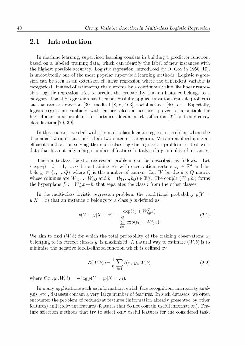
2.1 Introduction
In machine learning, supervised learning consists in building a predictor function,based on a labeled training data, which can identify the label of new instances withthe highest possible accuracy. Logistic regression, introduced by D. Cox in 1958 [19],is undoubtedly one of the most popular supervised learning methods. Logistic regres-sion can be seen as an extension of linear regression where the dependent variable iscategorical. Instead of estimating the outcome by a continuous value like linear regres-sion, logistic regression tries to predict the probability that an instance belongs to acategory. Logistic regression has been successfully applied in various real-life problemssuch as cancer detection [39], medical [8, 6, 103], social science [40], etc. Especially,logistic regression combined with feature selection has been proved to be suitable forhigh dimensional problems, for instance, document classification [27] and microarrayclassification [70, 39].
In this chapter, we deal with the multi-class logistic regression problem where thedependent variable has more than two outcome categories. We aim at developing anefficient method for solving the multi-class logistic regression problem to deal withdata that has not only a large number of features but also a large number of instances.
The multi-class logistic regression problem can be described as follows. Let(xi, yi) : i = 1, ..., n be a training set with observation vectors xi ∈ Rd and la-bels yi ∈ 1, ..., Q where Q is the number of classes. Let W be the d × Q matrixwhose columns are W:,1, ...,W:,Q and b = (b1, ..., bQ) ∈ RQ. The couple (W:,i, bi) formsthe hyperplane fi := W T
:,ix+ bi that separates the class i from the other classes.
In the multi-class logistic regression problem, the conditional probability p(Y =y|X = x) that an instance x belongs to a class y is defined as
p(Y = y|X = x) =exp(by +W T
:,yx)Q∑k=1
exp(bk +W T:,kx)
. (2.1)
We aim to find (W, b) for which the total probability of the training observations xibelonging to its correct classes yi is maximized. A natural way to estimate (W, b) is tominimize the negative log-likelihood function which is defined by
L(W, b) :=1
n
n∑i=1
`(xi, yi,W, b), (2.2)
where `(xi, yi,W, b) = − log p(Y = yi|X = xi).
In many applications such as information retrial, face recognition, microarray anal-ysis, etc., datasets contain a very large number of features. In such datasets, we oftenencounter the problem of redundant features (information already presented by otherfeatures) and irrelevant features (features that do not contain useful information). Fea-ture selection methods that try to select only useful features for the considered task,

Group Variable Selection in Multi-class Logistic Regression 41
is a popular and efficient way to deal with this problem. A natural way to deal withfeature selection problem is to formulate it as a minimization of the `0-norm (or ‖.‖0)where the `0-norm of x ∈ Rd is defined by the number of non-zero components of x,namely, ‖x‖0 = |i = 1, . . . , n : xi 6= 0|. It is well-known that the problem of minimiz-ing `0-norm is NP-hard [3] due to the discontinuity of `0-norm. The minimizationof `0-norm has been extensively studied on both theoretical and practical aspects forindividual variable selection in many practical problems. An extensive overview ofexisting approaches for the minimization of `0-norm can be found in [63].
In our problem, as mentioned above, the class i (i = 1, . . . , Q) is separated fromthe other classes by the hyperplane fi = W T
:,ix+ bi. If the weight Wj,i is equal to zerothen we can say that the feature j (j = 1, . . . , d) is not necessary to separate class ifrom the other classes. Hence, the feature j is to be removed if and only if it is notnecessary for any separator fi (i = 1, . . . , Q), i.e. all components in the row j of Ware zero. Therefore, it is reasonable to consider rows of W as groups. Denote by Wj,:
the j-th row of the matrix W . The `q,0-norm of W , i.e., the number of non-zero rowsof W , is defined by
‖W‖q,0 = |j ∈ 1, ..., d : ‖Wj,:‖q 6= 0|.
Hence, the `q,0 regularized multi-class logistic regression problem is formulated as fol-lows
minW,b
1
n
n∑i=1
`(xi, yi,W, b) + λ‖W‖q,0
. (2.3)
Our contributions
In this chapter, we investigate DC programming and DCA and propose two ap-proaches for solving the problem (2.3). As mentioned above, the regularization term`q,0 makes the problem (2.3) non-smooth non-convex. Hence, we first reformulated theproblem as a DC program, which DCA-based algorithms will be developed to solve it.We exploit the special structure of the problem to propose an efficient DC decompo-sition for which the corresponding DCA scheme is very inexpensive: it only requiresthe projection of points onto balls that is explicitly computed. Next, we considers twoapproaches based on advanced DC algorithms to efficiently solve it.
The first approach is suitable for large-scale setting, as it can exploit the advantageof the sum structure of (2.3). The proposed alogrithm, SDCA, is a Stochastic DCAfor the multi-class logistic regression with group variable selection. SDCA requires onlya small subset of components `(xi, yi,W, b) at each iteration instead of using all ncomponents for the calculation of W and b. We perform an empirical comparison ofSDCA with standard methods on very large synthetic and real-world datasets, and showthat SDCA is efficient in group variable selection ability and classification accuracy aswell as running time.
In the second approach, we considered another advanced DC algorithms (DCA-Like and Accelerated DCA-Like) for the problem (2.3). In standard DCA, the second
42 Group Variable Selection in Multi-class Logistic Regression
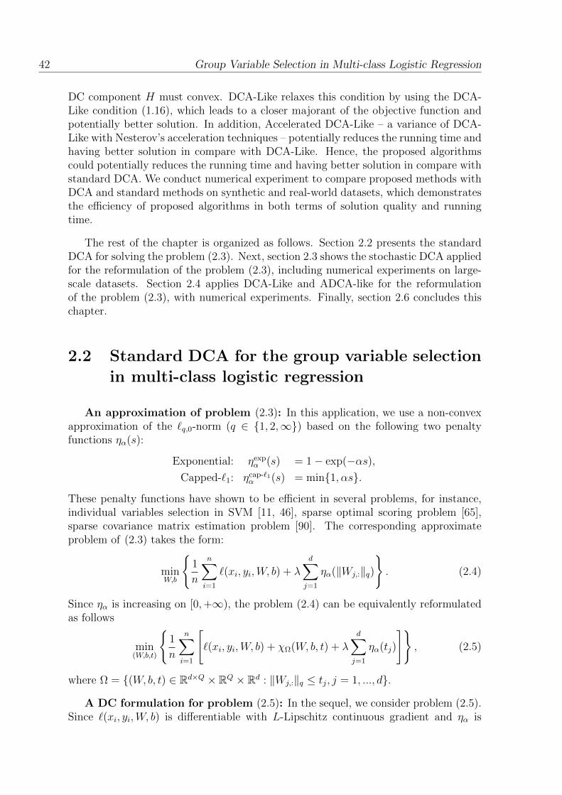
DC component H must convex. DCA-Like relaxes this condition by using the DCA-Like condition (1.16), which leads to a closer majorant of the objective function andpotentially better solution. In addition, Accelerated DCA-Like – a variance of DCA-Like with Nesterov’s acceleration techniques – potentially reduces the running time andhaving better solution in compare with DCA-Like. Hence, the proposed algorithmscould potentially reduces the running time and having better solution in compare withstandard DCA. We conduct numerical experiment to compare proposed methods withDCA and standard methods on synthetic and real-world datasets, which demonstratesthe efficiency of proposed algorithms in both terms of solution quality and runningtime.
The rest of the chapter is organized as follows. Section 2.2 presents the standardDCA for solving the problem (2.3). Next, section 2.3 shows the stochastic DCA appliedfor the reformulation of the problem (2.3), including numerical experiments on large-scale datasets. Section 2.4 applies DCA-Like and ADCA-like for the reformulationof the problem (2.3), with numerical experiments. Finally, section 2.6 concludes thischapter.
2.2 Standard DCA for the group variable selection
in multi-class logistic regression
An approximation of problem (2.3): In this application, we use a non-convexapproximation of the `q,0-norm (q ∈ 1, 2,∞) based on the following two penaltyfunctions ηα(s):
Exponential: ηexpα (s) = 1− exp(−αs),
Capped-`1: ηcap-`1α (s) = min1, αs.
These penalty functions have shown to be efficient in several problems, for instance,individual variables selection in SVM [11, 46], sparse optimal scoring problem [65],sparse covariance matrix estimation problem [90]. The corresponding approximateproblem of (2.3) takes the form:
minW,b
1
n
n∑i=1
`(xi, yi,W, b) + λ
d∑j=1
ηα(‖Wj,:‖q)
. (2.4)
Since ηα is increasing on [0,+∞), the problem (2.4) can be equivalently reformulatedas follows
min(W,b,t)
1
n
n∑i=1
[`(xi, yi,W, b) + χΩ(W, b, t) + λ
d∑j=1
ηα(tj)
], (2.5)
where Ω = (W, b, t) ∈ Rd×Q × RQ × Rd : ‖Wj,:‖q ≤ tj, j = 1, ..., d.
A DC formulation for problem (2.5): In the sequel, we consider problem (2.5).Since `(xi, yi,W, b) is differentiable with L-Lipschitz continuous gradient and ηα is
Group Variable Selection in Multi-class Logistic Regression 43
concave, the problem (2.5) takes the form of (1.11) where f(W, b) =∑n
i=1 `(xi, yi,W, b)and hj(tj) = ληα(tj)
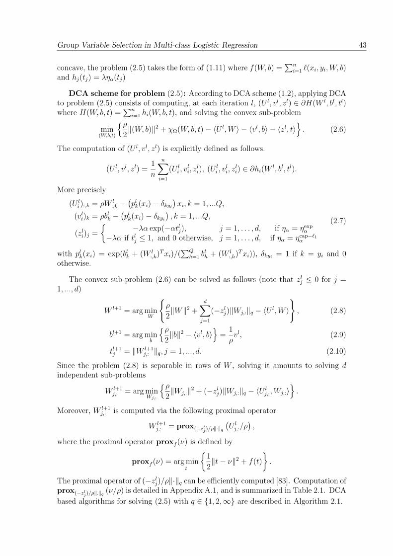
DCA scheme for problem (2.5): According to DCA scheme (1.2), applying DCAto problem (2.5) consists of computing, at each iteration l, (U l, vl, zl) ∈ ∂H(W l, bl, tl)where H(W, b, t) =
∑ni=1 hi(W, b, t), and solving the convex sub-problem
min(W,b,t)
ρ2‖(W, b)‖2 + χΩ(W, b, t)− 〈U l,W 〉 − 〈vl, b〉 − 〈zl, t〉
. (2.6)
The computation of (U l, vl, zl) is explicitly defined as follows.
(U l, vl, zl) =1
n
n∑i=1
(U li , v
li, z
li), (U l
i , vli, z
li) ∈ ∂hi(W l, bl, tl).
More precisely
(U li ):,k = ρW l
:,k −(plk(xi)− δkyi
)xi, k = 1, ...Q,
(vli)k = ρblk −(plk(xi)− δkyi
), k = 1, ...Q,
(zli)j =
−λα exp(−αtlj), j = 1, . . . , d, if ηα = ηexp
α
−λα if tlj ≤ 1, and 0 otherwise, j = 1, . . . , d, if ηα = ηcap−`1α
(2.7)
with plk(xi) = exp(blk + (W l:,k)
Txi)/(∑Q
h=1 blh + (W l
:,h)Txi)), δkyi = 1 if k = yi and 0
otherwise.
The convex sub-problem (2.6) can be solved as follows (note that zlj ≤ 0 for j =1, ..., d)
W l+1 = arg minW
ρ
2‖W‖2 +
d∑j=1
(−zlj)‖Wj,:‖q − 〈U l,W 〉
, (2.8)
bl+1 = arg minb
ρ2‖b‖2 − 〈vl, b〉
=
1
ρvl, (2.9)
tl+1j = ‖W l+1
j,: ‖q, j = 1, ..., d. (2.10)
Since the problem (2.8) is separable in rows of W , solving it amounts to solving dindependent sub-problems
W l+1j,: = arg min
Wj,:
ρ2‖Wj,:‖2 + (−zlj)‖Wj,:‖q − 〈U l
j,:,Wj,:〉.
Moreover, W l+1j,: is computed via the following proximal operator
W l+1j,: = prox(−zlj)/ρ‖·‖q
(U lj,:/ρ
),
where the proximal operator proxf (ν) is defined by
proxf (ν) = arg mint
1
2‖t− ν‖2 + f(t)
.
The proximal operator of (−zlj)/ρ‖·‖q can be efficiently computed [83]. Computation ofprox(−zlj)/ρ‖.‖q
(ν/ρ) is detailed in Appendix A.1, and is summarized in Table 2.1. DCA
based algorithms for solving (2.5) with q ∈ 1, 2,∞ are described in Algorithm 2.1.
44 Group Variable Selection in Multi-class Logistic Regression
Table 2.1 – Computation of W l+1j,: = prox(−zlj)/ρ‖.‖q
(U lj,:/ρ
)corresponding to q ∈
1, 2,∞.
q prox(−zlj)/ρ‖.‖q(U lj,:/ρ
)1
(|U l
j,:|/ρ− (−zlj)/ρ)
+ sign(U l
j,:)
2
(
1− −zlj‖U lj,:‖2
)U lj,:/ρ if ‖U l
j,:‖2 > −zlj0 if ‖U l
j,:‖2 ≤ −zlj.
∞
U lj,:/ρ−
(1−zlj|U l
j,:| − δ)
+ sign(U l
j,:) if ‖U lj,:‖1 > −zlj
0 if ‖U lj,:‖1 ≤ −zlj,
where δ satisfies∑Q
k=1
(1−zlj|U l
j,k| − δ)
+= 1.
Algorithm 2.1 DCA-`q,0: DCA for solving (2.5) with q ∈ 1, 2,∞Initialization: Choose (W 0, b0) ∈ Rd×Q × RQ, ρ > L and l← 0.Repeat
1. Compute (U l, vl, zl) = 1n
∑ni=1(U l
i , vli, z
li), where (U l
i , vli, z
li), i = 1, ..., n are
computed by defined in (2.7).2. Compute (W l+1, bl+1, tl+1) according to Table 2.1, (2.9) and (2.10), respec-
tively.3. l← l + 1.
Until Stopping criterion.
2.3 SDCA for the group variable selection in multi-
class logistic regression
Rewrite problem (2.5) into the form of (1.7): Since `(xi, yi,W, b) is differen-tiable with L-Lipschitz continuous gradient and ηα is concave, the problem (2.5) takesthe form of (1.7) where the function Fi(W, b, t) is given by
Fi(W, b, t) := gi(W, b, t)− hi(W, b, t)
where
gi(W, b, t) =ρ
2‖(W, b)‖2 + χΩ(W, b, t),
hi(W, b, t) =ρ
2‖(W, b)‖2 − `(xi, yi,W, b)− λ
d∑j=1
ηα(tj),
with ρ > L.

Group Variable Selection in Multi-class Logistic Regression 45
SDCA scheme for problem (2.5): Following SDCA in section 1.2, at eachiteration l, we have to compute (U l
i , vli, z
li) ∈ ∂hi(W
l, bl, tl) for i ∈ sl and keep(U l
i , vli, z
li) = (U l−1
i , vl−1i , zl−1
i ) for i /∈ sl, where sl is a randomly chosen subset ofthe indexes, and solve the convex sub-problem taking the form of (2.6). This is themain speed-up of SDCA in comparison with DCA. In standard DCA in section 2.7,the most expensive operation is the computing the subgradient (U l, vl) =
∑ni (Ui, vi),
which is linearly scale with n. In contrast, SDCA only uses a subset sl to compute(U l, vl) =
∑i∈sl (Ui, vi), which significantly reduces the computing time of this bottle-
neck. It is clear that each iteration of SDCA is much faster than DCA, hence SDCAis potentially faster than DCA.
SDCA for solving (2.5) is described in Algorithm 2.2.
Algorithm 2.2 SDCA-`q,0: SDCA for solving (2.5) with q ∈ 1, 2,∞Initialize:
Choose (W 0, b0) ∈ Rd×Q × RQ, t0j = ‖W 0j,:‖q, ρ > L, s0 = 1, ..., n
and l← 0.repeat
1. Compute (U li , v
li, z
li) by (2.7) if i ∈ sl and keep (U l
i , vli, z
li) = (U l−1
i , vl−1i , zl−1
i )if i /∈ sl. Set (U l, vl, zl) = 1
n
∑ni=1(U l
i , vli, z
li).
2. Compute (W l+1, bl+1, tl+1) according to Table 2.1, (2.9) and (2.10), respec-tively.
3. l← l + 1 and randomly choose a small subset sl ⊂ 1, ..., n.until Stopping criterion.
2.3.1 Numerical experiment
2.3.1.1 Datasets
To evaluate the performances of algorithms, we performed numerical experimentson two types of data: real datasets (covertype, madelon, miniboone, protein, sensit andsensorless) and simulated datasets (sim 1, sim 2 and sim 3 ). All real-world datasetsare taken from the well-known UCI and LibSVM data repositories. We give below abrief description of real datasets:
— covertype belongs to the Forest Cover Type Prediction from strictly cartographicvariables challenge 2. It is a very large dataset containing 581, 012 points de-scribed by 54 variables.
— madelon is one of five datasets used in the NIPS 2003 feature selection chal-lenge 3. The dataset contains 2600 points, each point is represented by 500variables. Among 500 variables, there are only 5 informative variables and 15redundant variables (which are created by linear combinations of 5 informative
2. https://archive.ics.uci.edu/ml/datasets/Covertype
3. https://archive.ics.uci.edu/ml/datasets/Madelon

46 Group Variable Selection in Multi-class Logistic Regression
variables). The 480 others variables were added and have no predictive power.Notice that madelon is a highly non-linear dataset.
— miniboone is taken form the MiniBooNE experiment to observe neutrino oscil-lations 4, containing 130, 065 data points.
— protein 5 is a dataset for classifying protein second structure state (α, β, andcoil) of each residue in amino acid sequences, including 24, 387 data points.
— sensit 5 dataset obtained from distributed sensor network for vehicle classifi-cation. It consists of 98, 528 data points categorized into 3 classes: AssaultAmphibian Vehicle (AAV), Dragon Wagon (DW) and noise.
— sensorless measures electric current drive signals from different operating con-ditions, which is classified into 11 different classes 6. It is a huge dataset, whichcontains 58, 509 data points, described by 48 variables.
We generate three synthetic datasets (sim 1, sim 2 and sim 3 ) by the same processproposed in [115]. In the first dataset (sim 1 ), variables are independent and havedifferent means in each class. In dataset (sim 2 ), variables also have different meansin each class, but they are dependent. The last synthetic dataset (sim 3 ) has differentone-dimensional means in each class with independent variables. Detail produces togenerate three simulated datasets are described as follows:
— For sim 1 : we generate a four-classes classification problem. Each class isassumed to have a multivariate normal distribution N (µk, I), k = 1, 2, 3, 4 withdimension of d = 50. The first 10 components of µ1 are 0.5, µ2j = 0.5 if11 ≤ j ≤ 20, µ3j = 0.5 if 21 ≤ j ≤ 30, µ4j = 0.5 if 31 ≤ j ≤ 40 and 0 otherwise.We generate 100, 000 instances with equal probabilities.
— For sim 2 : this synthetic dataset contains three classes of multivariate normaldistributions N (µk,Σ), k = 1, 2, 3, each of dimension d = 50. The componentsof µ1 = 0, µ2j = 0.4 and µ3j = 0.8 if j ≤ 40 and 0 otherwise. The covariancematrix Σ is the block diagonal matrix with five blocks of dimension 10 × 10whose element (j, j′) is 0.6|j−j
′|. We generate 150, 000 instances.— For sim 3 : this synthetic dataset consists of four classes. For class k = 1, 2, 3, 4,
i ∈ Ck then Xij ∼ N (0, 1) for j > 100, and Xij ∼ N (k−13, 1) otherwise, where
N (µ, σ2) denotes the Gaussian distribution with mean µ and variance σ2. Wegenerate 62, 500 data points for each class.
The number of points, variables and classes of each dataset are summarized in thefirst column of Table 2.2.
2.3.1.2 Comparative algorithms
To the best of our knowledge, there is no existing method in the literature for solvingthe group variable selection in multi-class logistic regression using `q,0 regularization.However, closely connected to the Lasso (`1-norm), [109] proposed to use the convex
4. https://archive.ics.uci.edu/ml/datasets/MiniBooNE+particle+identification
5. https://www.csie.ntu.edu.tw/~cjlin/libsvmtools/datasets/multiclass.html
6. https://archive.ics.uci.edu/ml/datasets/Dataset+for+Sensorless+Drive+Diagnosis

Group Variable Selection in Multi-class Logistic Regression 47
regularization `2,1 instead of `2,0. Thus, the resulting problem takes the form
minW,b
1
n
n∑i=1
`(xi, yi,W, b) + λ‖W‖2,1
. (2.11)
A coordinate gradient descent method, named msgl, was proposed in [109] to solvethe problem (2.11). msgl is a comparative algorithm in our experiment.
On another hand, we are interested in a comparison between our algorithms anda stochastic based method. A stochastic gradient descent algorithm to solve (2.11),named SPGD-`2,1, is developed for this purpose. SPGD-`2,1 is described as follows.
Algorithm 2.3 SPGD-`2,1: Stochastic Proximal Gradient Descent for solving (2.11)
Initialization: Choose (W 0, b0) ∈ Rd×Q × RQ, and l← 0.Repeat
1. Randomly choose a small subset sl ⊂ 1, ..., n. Set αl = n10l
. ComputeU l
:,k = W l:,k −
αl|sl|∑
i∈sl
(plk(xi)− δkyi
)xi, k = 1, ...Q.
2. Compute (W l+1, bl+1) by
W l+1j,: =
(‖U l
j,:‖2 − αlλ)
+
U lj,:
‖U lj,:‖2
, j = 1, ..., d
bl+1k = blk −
αl|sl|∑i∈sl
(plk(xi)− δkyi
), k = 1, ..., Q.
(2.12)
3. l← l + 1.Until Stopping criterion.
2.3.1.3 Experiment setting
We randomly split each dataset into a training set and a test set. The training setcontains 80% of the total number of points and the remaining 20% are used as testset.
In order to evaluate the performance of algorithms, we consider the following threecriteria: the classification accuracy (percentage of well classified point on test set), thesparsity of obtained solution and the running time (measured in seconds). The sparsityis computed as the percentage of selected variables. Note that a variable j ∈ 1, . . . , dis considered to be removed if all components of the row j of W are smaller than athreshold, i.e., |Wj,i| ≤ 10−8,∀i ∈ 1, . . . , Q. We perform each algorithm 10 times andreport the mean and standard deviation of each criterion.
We use the early-stopping condition for SDCA and SPGD-`2,1. Early-stopping isa well-know technique in machine learning, especially in stochastic learning whichpermits to avoid the over-fitting in learning. More precisely, after each epoch, wecompute the classification accuracy on a validation set which contains 20% randomly

48 Group Variable Selection in Multi-class Logistic Regression
chosen data points of training set. We stop SDCA and SPGD-`2,1 if the classificationaccuracy is not improved after npatience = 5 epochs. The batch size of stochasticalgorithms (SDCA and SPGD-`2,1) is set to 10%. DCA is stopped if the difference betweentwo consecutive objective functions is smaller than a threshold εstop = 10−6. For msgl,we use its default stopping parameters as in [109]. We also stop algorithms if theyexceed 2 hours of running time in the training process.
The parameter α for controlling the tightness of zero-norm approximation is chosenin the set 0.5, 1, 2, 5. We use the solution-path procedure for the trade-off parameterλ. Let λ1 > λ2 > ... > λl be a decreasing sequence of λ. At step k, we solve theproblem (2.3) with λ = λk from the initial point chosen as the solution of the previousstep k − 1. Starting with a large value of λ, we privilege the sparsity of solution (i.e.selecting very few variables) over the classification ability. Then by decreasing the valueλ decreases, we select more variables in order to increase the classification accuracy.In our experiments, the sequence of λ is set to 104, 3× 10³, 103, . . . , 3× 10⁻³, 10−3.
All experiments are performed on a PC Intel (R) Xeon (R) E5-2630 v2 @2.60 GHzwith 32GB RAM.
2.3.1.4 Experiment 1
In this experiments, we study the effectiveness of SDCA. For this purpose, wechoose the `2,0 regularization, and perform a comparison between SDCA-`2,0-exp andDCA-`2,0-exp. Furthermore, we will compare SDCA-`2,0-exp with msgl and SPGD-`2,1,two algorithms for solving the multi-class logistic regression using `2,1 regularization(c.f Section 2.3.1.2).
The comparative results between are reported in Table 2.2 and Figure 2.1. Notethat the running time is plotted in logarithmic scale.
Comparison between SDCA-`2,0 and DCA-`2,0-exp
In term of classification accuracy, SDCA-`2,0-exp produces fairly similar result com-paring with DCA-`2,0-exp. DCA-`2,0-exp is better than SDCA-`2,0-exp on 4 datasets(covertype, sensit, sensorless and sim 3 ) while SDCA-`1,0-exp gives better results on 2datasets (madelon and protein). The two biggest gaps (3.49% and 1.17%) occur ondataset sensorless and sensit respectively.
As for the sparsity of solution, DCA-`2,0-exp and SDCA-`2,0-exp provide the sameresults on 4 datasets (miniboon, sim 1, sim 2 and sim 3 ). DCA-`2,0-exp suppressesmore variables than SDCA-`2,0-exp on 3 datasets (protein, sensit and sensorless),while SDCA-`2,0-exp gives better sparsity on covertype and madelon. The gain ofDCA-`2,0-exp on this criterion is quite high, up to 22.3% on dataset protein.
Concerning the running time, SDCA-`2,0-exp clearly outperforms DCA-`2,0-exp. Ex-cept for miniboone where DCA-`2,0-exp is 1.11 second faster, the gain of SDCA-`2,0-exp
is huge. SDCA-`2,0-exp is up to 19.58 times faster than DCA-`2,0-exp (dataset cover-

Group Variable Selection in Multi-class Logistic Regression 49
60 65 70 75 80 85 90 95 100
Accuracy (%)
sim_3
sim_2
sim_1
sensorless
sensit
protein
miniboone
madelon
covertype SDCA-ℓ2,0SPGD-ℓ2,1DCA-ℓ2,0msgl
0 10 20 30 40 50 60 70 80 90 100
Sparsity (%)
sim_3
sim_2
sim_1
sensorless
sensit
protein
miniboone
madelon
covertype
SDCA-ℓ2,0SPGD-ℓ2,1DCA-ℓ2,0msgl
10-1 100 101 102 103 104
Time (sec)
sim_3
sim_2
sim_1
sensorless
sensit
protein
miniboone
madelon
covertype SDCA-ℓ2,0SPGD-ℓ2,1DCA-ℓ2,0msgl
Figure 2.1 – Comparative results between SDCA-`2,0-exp, DCA-`2,0-exp, SPGD-`2,1
and msgl (running time is plotted on a logarithmic scale).
type).
Overall, SDCA-`2,0-exp is able to achieve equivalent classification accuracy with a
... I: : 1
1 1 1 1 1 1 1 1
~
~ --c=J c=J
1 1 1 1
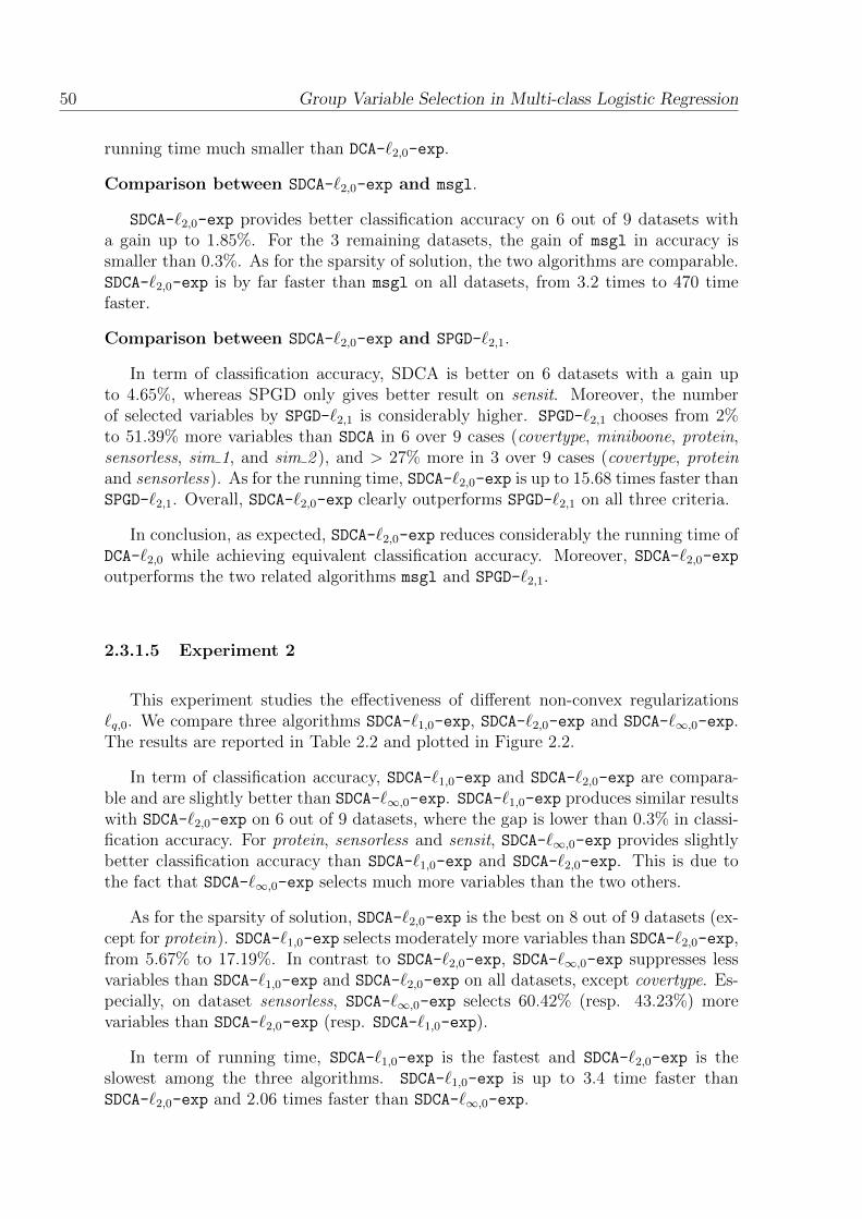
50 Group Variable Selection in Multi-class Logistic Regression
running time much smaller than DCA-`2,0-exp.
Comparison between SDCA-`2,0-exp and msgl.
SDCA-`2,0-exp provides better classification accuracy on 6 out of 9 datasets witha gain up to 1.85%. For the 3 remaining datasets, the gain of msgl in accuracy issmaller than 0.3%. As for the sparsity of solution, the two algorithms are comparable.SDCA-`2,0-exp is by far faster than msgl on all datasets, from 3.2 times to 470 timefaster.
Comparison between SDCA-`2,0-exp and SPGD-`2,1.
In term of classification accuracy, SDCA is better on 6 datasets with a gain upto 4.65%, whereas SPGD only gives better result on sensit. Moreover, the numberof selected variables by SPGD-`2,1 is considerably higher. SPGD-`2,1 chooses from 2%to 51.39% more variables than SDCA in 6 over 9 cases (covertype, miniboone, protein,sensorless, sim 1, and sim 2 ), and > 27% more in 3 over 9 cases (covertype, proteinand sensorless). As for the running time, SDCA-`2,0-exp is up to 15.68 times faster thanSPGD-`2,1. Overall, SDCA-`2,0-exp clearly outperforms SPGD-`2,1 on all three criteria.
In conclusion, as expected, SDCA-`2,0-exp reduces considerably the running time ofDCA-`2,0 while achieving equivalent classification accuracy. Moreover, SDCA-`2,0-exp
outperforms the two related algorithms msgl and SPGD-`2,1.
2.3.1.5 Experiment 2
This experiment studies the effectiveness of different non-convex regularizations`q,0. We compare three algorithms SDCA-`1,0-exp, SDCA-`2,0-exp and SDCA-`∞,0-exp.The results are reported in Table 2.2 and plotted in Figure 2.2.
In term of classification accuracy, SDCA-`1,0-exp and SDCA-`2,0-exp are compara-ble and are slightly better than SDCA-`∞,0-exp. SDCA-`1,0-exp produces similar resultswith SDCA-`2,0-exp on 6 out of 9 datasets, where the gap is lower than 0.3% in classi-fication accuracy. For protein, sensorless and sensit, SDCA-`∞,0-exp provides slightlybetter classification accuracy than SDCA-`1,0-exp and SDCA-`2,0-exp. This is due tothe fact that SDCA-`∞,0-exp selects much more variables than the two others.
As for the sparsity of solution, SDCA-`2,0-exp is the best on 8 out of 9 datasets (ex-cept for protein). SDCA-`1,0-exp selects moderately more variables than SDCA-`2,0-exp,from 5.67% to 17.19%. In contrast to SDCA-`2,0-exp, SDCA-`∞,0-exp suppresses lessvariables than SDCA-`1,0-exp and SDCA-`2,0-exp on all datasets, except covertype. Es-pecially, on dataset sensorless, SDCA-`∞,0-exp selects 60.42% (resp. 43.23%) morevariables than SDCA-`2,0-exp (resp. SDCA-`1,0-exp).
In term of running time, SDCA-`1,0-exp is the fastest and SDCA-`2,0-exp is theslowest among the three algorithms. SDCA-`1,0-exp is up to 3.4 time faster thanSDCA-`2,0-exp and 2.06 times faster than SDCA-`∞,0-exp.
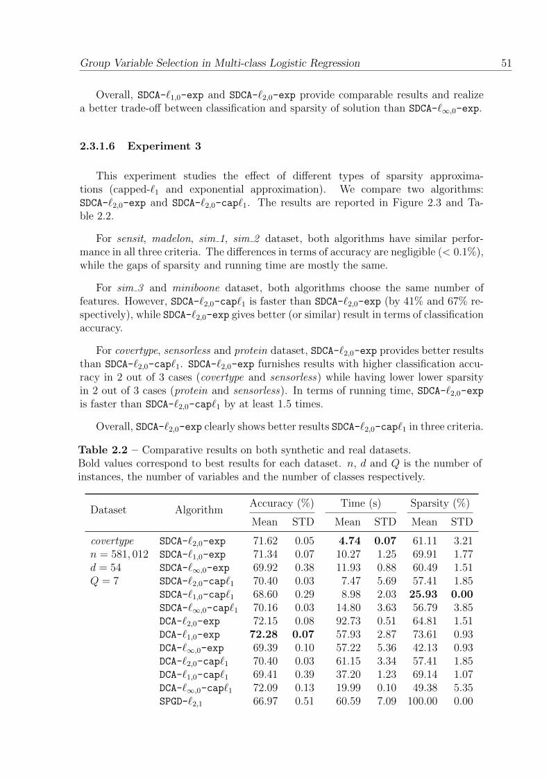
Group Variable Selection in Multi-class Logistic Regression 51
Overall, SDCA-`1,0-exp and SDCA-`2,0-exp provide comparable results and realizea better trade-off between classification and sparsity of solution than SDCA-`∞,0-exp.
2.3.1.6 Experiment 3
This experiment studies the effect of different types of sparsity approxima-tions (capped-`1 and exponential approximation). We compare two algorithms:SDCA-`2,0-exp and SDCA-`2,0-cap`1. The results are reported in Figure 2.3 and Ta-ble 2.2.
For sensit, madelon, sim 1, sim 2 dataset, both algorithms have similar perfor-mance in all three criteria. The differences in terms of accuracy are negligible (< 0.1%),while the gaps of sparsity and running time are mostly the same.
For sim 3 and miniboone dataset, both algorithms choose the same number offeatures. However, SDCA-`2,0-cap`1 is faster than SDCA-`2,0-exp (by 41% and 67% re-spectively), while SDCA-`2,0-exp gives better (or similar) result in terms of classificationaccuracy.
For covertype, sensorless and protein dataset, SDCA-`2,0-exp provides better resultsthan SDCA-`2,0-cap`1. SDCA-`2,0-exp furnishes results with higher classification accu-racy in 2 out of 3 cases (covertype and sensorless) while having lower lower sparsityin 2 out of 3 cases (protein and sensorless). In terms of running time, SDCA-`2,0-exp
is faster than SDCA-`2,0-cap`1 by at least 1.5 times.
Overall, SDCA-`2,0-exp clearly shows better results SDCA-`2,0-cap`1 in three criteria.
Table 2.2 – Comparative results on both synthetic and real datasets.Bold values correspond to best results for each dataset. n, d and Q is the number ofinstances, the number of variables and the number of classes respectively.
Dataset AlgorithmAccuracy (%) Time (s) Sparsity (%)
Mean STD Mean STD Mean STD
covertype SDCA-`2,0-exp 71.62 0.05 4.74 0.07 61.11 3.21n = 581, 012 SDCA-`1,0-exp 71.34 0.07 10.27 1.25 69.91 1.77d = 54 SDCA-`∞,0-exp 69.92 0.38 11.93 0.88 60.49 1.51Q = 7 SDCA-`2,0-cap`1 70.40 0.03 7.47 5.69 57.41 1.85
SDCA-`1,0-cap`1 68.60 0.29 8.98 2.03 25.93 0.00SDCA-`∞,0-cap`1 70.16 0.03 14.80 3.63 56.79 3.85DCA-`2,0-exp 72.15 0.08 92.73 0.51 64.81 1.51DCA-`1,0-exp 72.28 0.07 57.93 2.87 73.61 0.93DCA-`∞,0-exp 69.39 0.10 57.22 5.36 42.13 0.93DCA-`2,0-cap`1 70.40 0.03 61.15 3.34 57.41 1.85DCA-`1,0-cap`1 69.41 0.39 37.20 1.23 69.14 1.07DCA-`∞,0-cap`1 72.09 0.13 19.99 0.10 49.38 5.35SPGD-`2,1 66.97 0.51 60.59 7.09 100.00 0.00
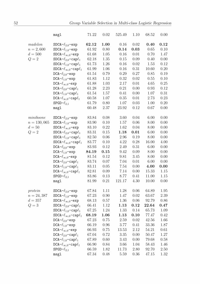
52 Group Variable Selection in Multi-class Logistic Regression
msgl 71.22 0.02 525.49 1.10 68.52 0.00
madelon SDCA-`2,0-exp 62.12 1.00 0.16 0.02 0.40 0.12n = 2, 600 SDCA-`1,0-exp 61.92 0.80 0.14 0.03 0.65 0.10d = 500 SDCA-`∞,0-exp 61.68 1.05 0.16 0.01 0.70 1.47Q = 2 SDCA-`2,0-cap`1 62.18 1.35 0.15 0.09 0.40 0.00
SDCA-`1,0-cap`1 61.73 1.26 0.16 0.02 1.53 0.12SDCA-`∞,0-cap`1 61.99 1.06 0.16 0.31 10.60 0.20DCA-`2,0-exp 61.54 0.79 0.29 0.27 0.85 0.19DCA-`1,0-exp 61.83 1.12 0.32 0.02 0.55 0.10DCA-`∞,0-exp 61.88 1.03 2.17 0.01 4.65 0.25DCA-`2,0-cap`1 61.28 2.23 0.21 0.00 0.93 0.12DCA-`1,0-cap`1 61.54 1.57 0.41 0.00 1.07 0.31DCA-`∞,0-cap`1 60.58 1.07 0.35 0.01 2.73 0.23SPGD-`2,1 61.79 0.80 1.07 0.03 1.00 0.20msgl 60.48 2.37 23.92 0.12 0.67 0.00
miniboone SDCA-`2,0-exp 83.84 0.08 3.60 0.04 6.00 0.00n = 130, 065 SDCA-`1,0-exp 83.90 0.10 1.57 0.06 8.00 0.00d = 50 SDCA-`∞,0-exp 83.10 0.22 1.62 0.04 8.00 0.00Q = 2 SDCA-`2,0-cap`1 83.31 0.15 1.18 0.01 6.00 0.00
SDCA-`1,0-cap`1 82.50 0.06 2.96 0.19 8.00 0.00SDCA-`∞,0-cap`1 83.77 0.10 4.22 0.28 16.00 4.00DCA-`2,0-exp 83.93 0.12 2.49 0.31 6.00 0.00DCA-`1,0-exp 84.19 0.15 9.42 0.09 8.00 0.00DCA-`∞,0-exp 81.54 0.12 9.81 3.45 8.00 0.00DCA-`2,0-cap`1 83.74 0.07 7.04 0.01 6.00 0.00DCA-`1,0-cap`1 83.11 0.05 7.54 0.00 4.00 0.00DCA-`∞,0-cap`1 82.81 0.09 7.14 0.00 15.33 1.15SPGD-`2,1 83.86 0.13 8.77 0.41 11.00 1.15msgl 81.99 0.21 121.17 4.30 10.00 0.00
protein SDCA-`2,0-exp 67.84 1.11 1.28 0.06 64.89 1.95n = 24, 387 SDCA-`1,0-exp 67.23 0.90 1.47 0.02 63.67 2.39d = 357 SDCA-`∞,0-exp 68.13 0.57 1.36 0.06 92.79 0.86Q = 3 SDCA-`2,0-cap`1 66.41 1.12 1.13 0.12 22.64 0.47
SDCA-`1,0-cap`1 67.25 1.24 1.33 0.14 65.73 1.09SDCA-`∞,0-cap`1 68.19 1.06 1.13 0.10 77.47 0.42DCA-`2,0-exp 67.23 0.75 2.59 0.02 42.56 1.66DCA-`1,0-exp 66.19 0.96 3.77 0.41 33.36 1.87DCA-`∞,0-exp 66.93 0.75 13.53 2.12 54.21 0.61DCA-`2,0-cap`1 67.04 0.72 3.35 0.00 50.47 1.27DCA-`1,0-cap`1 67.89 0.60 3.43 0.00 79.68 0.58DCA-`∞,0-cap`1 66.90 0.84 3.66 1.04 58.43 1.46SPGD-`2,1 66.59 1.82 11.73 2.80 92.70 2.50msgl 67.34 0.48 5.59 0.36 47.15 1.32

Group Variable Selection in Multi-class Logistic Regression 53
sensit SDCA-`2,0-exp 78.67 0.11 3.48 0.21 28.33 8.50n = 98, 528 SDCA-`1,0-exp 79.64 0.22 3.11 0.96 34.00 17.35d = 100 SDCA-`∞,0-exp 79.73 0.28 1.61 0.07 53.67 6.81Q = 3 SDCA-`2,0-cap`1 78.59 0.08 2.94 0.17 33.80 5.31
SDCA-`1,0-cap`1 79.71 0.23 2.94 2.12 100.00 0.00SDCA-`∞,0-cap`1 78.83 0.24 2.91 0.20 35.00 2.74DCA-`2,0-exp 79.84 0.11 27.97 0.80 19.25 0.50DCA-`1,0-exp 79.65 0.21 18.31 4.90 17.50 0.58DCA-`∞,0-exp 79.16 0.17 42.91 5.24 91.50 2.38DCA-`2,0-cap`1 78.92 0.15 26.36 2.22 56.67 1.53DCA-`1,0-cap`1 78.91 0.38 27.05 2.80 57.33 0.58DCA-`∞,0-cap`1 79.20 0.17 35.78 2.69 91.67 7.23SPGD-`2,1 79.52 0.27 22.44 2.41 27.00 1.00msgl 79.02 0.13 11.16 0.53 23.00 0.00
sensorless SDCA-`2,0-exp 86.52 0.78 1.47 0.16 37.50 5.10n = 58, 509 SDCA-`1,0-exp 87.33 0.27 1.40 0.09 54.69 10.67d = 48 SDCA-`∞,0-exp 86.91 0.19 1.41 0.38 97.92 2.08Q = 11 SDCA-`2,0-cap`1 84.77 0.08 2.45 0.13 68.06 1.20
SDCA-`1,0-cap`1 82.89 0.30 2.69 0.62 72.92 2.08SDCA-`∞,0-cap`1 87.12 0.72 1.36 0.09 25.69 1.20DCA-`2,0-exp 90.00 0.31 15.96 0.65 32.81 1.04DCA-`1,0-exp 89.11 0.18 16.28 0.97 31.25 0.00DCA-`∞,0-exp 90.76 0.14 18.99 0.81 100.00 0.00DCA-`2,0-cap`1 89.60 1.15 24.75 1.39 53.47 1.20DCA-`1,0-cap`1 88.87 1.04 16.28 0.44 47.92 0.80DCA-`∞,0-cap`1 81.06 3.9 14.99 3.22 41.67 0.70SPGD-`2,1 86.07 1.39 8.16 1.05 88.89 2.41msgl 85.06 0.31 199.00 41.75 50.00 0.00
sim 1 SDCA-`2,0-exp 72.22 0.46 0.46 0.02 80.00 0.00n = 100, 000 SDCA-`1,0-exp 72.24 0.43 0.46 0.03 80.00 0.00d = 50 SDCA-`∞,0-exp 72.24 0.47 0.56 0.06 80.00 0.00Q = 4 SDCA-`2,0-cap`1 72.24 0.52 0.50 0.04 80.00 0.00
SDCA-`1,0-cap`1 72.24 0.58 0.42 0.06 80.00 0.00SDCA-`∞,0-cap`1 72.21 0.58 0.51 0.07 80.00 0.00DCA-`2,0-exp 72.22 0.40 2.34 0.05 80.00 0.00DCA-`1,0-exp 72.25 0.38 0.26 0.01 80.00 0.00DCA-`∞,0-exp 72.22 0.40 9.79 0.10 80.00 0.00DCA-`2,0-cap`1 72.25 0.52 0.32 0.00 80.00 0.00DCA-`1,0-cap`1 72.24 0.52 0.30 0.00 80.00 0.00DCA-`∞,0-cap`1 72.24 0.51 3.00 0.00 80.00 0.00SPGD-`2,1 71.48 0.81 7.16 0.91 83.50 2.52msgl 72.33 0.18 214.83 25.40 82.00 0.00
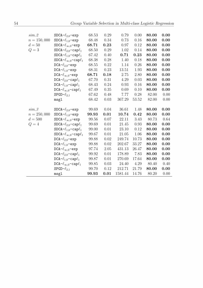
54 Group Variable Selection in Multi-class Logistic Regression
sim 2 SDCA-`2,0-exp 68.53 0.29 0.79 0.00 80.00 0.00n = 150, 000 SDCA-`1,0-exp 68.48 0.34 0.73 0.16 80.00 0.00d = 50 SDCA-`∞,0-exp 68.71 0.23 0.97 0.12 80.00 0.00Q = 3 SDCA-`2,0-cap`1 68.50 0.29 1.02 0.14 80.00 0.00
SDCA-`1,0-cap`1 67.42 0.40 0.71 0.23 80.00 0.00SDCA-`∞,0-cap`1 68.38 0.28 1.40 0.18 80.00 0.00DCA-`2,0-exp 68.55 0.22 1.14 0.26 80.00 0.00DCA-`1,0-exp 68.31 0.23 13.51 1.93 80.00 0.00DCA-`∞,0-exp 68.71 0.18 2.75 2.80 80.00 0.00DCA-`2,0-cap`1 67.70 0.31 4.29 0.03 80.00 0.00DCA-`1,0-cap`1 68.43 0.24 0.93 0.16 80.00 0.00DCA-`∞,0-cap`1 67.49 0.35 0.69 0.10 80.00 0.00SPGD-`2,1 67.62 0.48 7.77 0.28 82.00 0.00msgl 68.42 0.03 367.29 53.52 82.00 0.00
sim 3 SDCA-`2,0-exp 99.69 0.04 36.61 1.48 80.00 0.00n = 250, 000 SDCA-`1,0-exp 99.93 0.01 10.74 0.42 80.00 0.00d = 500 SDCA-`∞,0-exp 99.56 0.07 22.11 3.43 80.73 0.64Q = 4 SDCA-`2,0-cap`1 99.69 0.01 21.45 0.93 80.00 0.00
SDCA-`1,0-cap`1 99.00 0.01 23.10 0.12 80.00 0.00SDCA-`∞,0-cap`1 99.67 0.01 21.05 1.06 80.00 0.00DCA-`2,0-exp 99.88 0.02 249.74 10.73 80.00 0.00DCA-`1,0-exp 99.88 0.02 202.67 33.27 80.00 0.00DCA-`∞,0-exp 97.74 2.05 431.13 26.47 80.00 0.00DCA-`2,0-cap`1 99.92 0.01 178.89 7.83 80.00 0.00DCA-`1,0-cap`1 99.87 0.01 270.69 17.64 80.00 0.00DCA-`∞,0-cap`1 99.85 0.03 24.40 4.29 80.40 0.40SPGD-`2,1 99.70 0.12 212.71 21.79 80.00 0.00msgl 99.93 0.01 1581.44 14.76 80.20 0.00
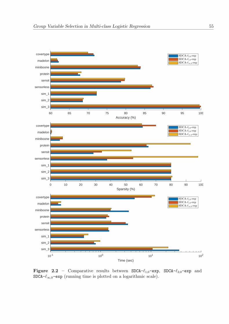
Group Variable Selection in Multi-class Logistic Regression 55
60 65 70 75 80 85 90 95 100
Accuracy (%)
sim_3
sim_2
sim_1
sensorless
sensit
protein
miniboone
madelon
covertype
0 10 20 30 40 50 60 70 80 90 100
Sparsity (%)
sim_3
sim_2
sim_1
sensorless
sensit
protein
miniboone
madelon
covertype
10-1 100 101 102
Time (sec)
sim_3
sim_2
sim_1
sensorless
sensit
protein
miniboone
madelon
covertype
Figure 2.2 – Comparative results between SDCA-`1,0-exp, SDCA-`2,0-exp andSDCA-`∞,0-exp (running time is plotted on a logarithmic scale).
- SDCA-€2,0-exp - SDCA-€1,0-exp c==J SDCA-€00,0-exp
1
- SDCA-€2,0-exp
i - SDCA-€1,0-exp c==J SDCA-t'oo,o-exp
r--
1 1
- SDCA-l 2,o-exp
~ - SDCA-€1,0-exp c==J SDCA-loo,o-exp
'

56 Group Variable Selection in Multi-class Logistic Regression
60 65 70 75 80 85 90 95 100
Accuracy (%)
sim_3
sim_2
sim_1
sensorless
sensit
protein
miniboone
madelon
covertype
0 10 20 30 40 50 60 70 80
Sparsity (%)
sim_3
sim_2
sim_1
sensorless
sensit
protein
miniboone
madelon
covertype
10-1 100 101 102
Time (sec)
sim_3
sim_2
sim_1
sensorless
sensit
protein
miniboone
madelon
covertype
Figure 2.3 – Comparative results between SDCA-`2,0-exp and SDCA-`2,0-cap`1 (run-ning time is plotted on a logarithmic scale).
- SDCA-C,,o-exp - SDCA-C2,0-capf1
- SDCA-f,,o-exp - SDCA-f2,0-capf1
- SDCA-f2,o-exp - SDCA-f2,o-capf1
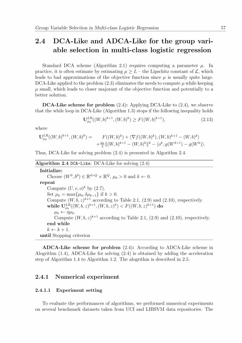
Group Variable Selection in Multi-class Logistic Regression 57
2.4 DCA-Like and ADCA-Like for the group vari-
able selection in multi-class logistic regression
Standard DCA scheme (Algorithm 2.1) requires computing a parameter µ. Inpractice, it is often estimate by estimating µ ≥ L – the Lipschitz constant of L, whichleads to bad approximations of the objective function since µ is usually quite large.DCA-Like applied to the problem (2.3) eliminates the needs to compute µ while keepingµ small, which leads to closer majorant of the objective function and potentially to abetter solution.
DCA-Like scheme for problem (2.4): Applying DCA-Like to (2.4), we observethat the while loop in DCA-Like (Algorithm 1.3) stops if the following inequality holds
ULRµk
((W, b)k+1, (W, b)k) ≥ F ((W, b)k+1), (2.13)
where
ULRµk
((W, b)k+1, (W, b)k) = F ((W, b)k) + 〈∇f((W, b)k), (W, b)k+1 − (W, b)k〉+µk
2‖(W, b)k+1 − (W, b)k‖2 − 〈ok, g(W k+1)− g(W k)〉.
Thus, DCA-Like for solving problem (2.4) is presented in Algorithm 2.4.
Algorithm 2.4 DCA-Like: DCA-Like for solving (2.4)
Initialize:Choose (W 0, b0) ∈ Rd×Q × RQ, µ0 > 0 and k ← 0.
repeatCompute (U, v, o)k by (2.7).Set µk = maxµ0, δµk−1 if k > 0.Compute (W, b, z)k+1 according to Table 2.1, (2.9) and (2.10), respectively.while ULR
µk((W, b, z)k+1, (W, b, z)k) < F ((W, b, z)k+1) do
µk ← ηµk.Compute (W, b, z)k+1 according to Table 2.1, (2.9) and (2.10), respectively.
end whilek ← k + 1.
until Stopping criterion
ADCA-Like scheme for problem (2.4): According to ADCA-Like scheme inAlogrithm (1.4), ADCA-Like for solving (2.4) is obtained by adding the accelerationstep of Algorithm 1.4 to Algorithm 1.2. The alogrithm is described in 2.5.
2.4.1 Numerical experiment
2.4.1.1 Experiment setting
To evaluate the performances of algorithms, we performed numerical experimentson several benchmark datasets taken from UCI and LIBSVM data repositories. The

58 Group Variable Selection in Multi-class Logistic Regression
Algorithm 2.5 ADCA-Like: ADCA-Like for solving (2.4)
Initialize:Choose (W 0, b0) ∈ Rd×Q × RQ, ω0 = W 0, β0 = b0,η > 1, 0 < δ < 1, µ0 > 0 and k ← 0.
repeatif F (ωk, βk) ≤ F (W k, bk) then
set wk = ωk and bk = βk
elseset wk = W k and bk = bk
end ifCompute (Uk, vk) = µ(wk,bk)− 1
n
∑ni=1∇`(xi, yi,wk,bk)
Compute okj ∈ ∂(−λ∑d
j=1 ηα(‖wkj,:‖2)
)for j = 1, . . . , d (similar to (2.7)).
Set µk = maxµ0, δµk−1 if k > 0.Compute (W, b, z)k+1 according to Table 2.1, (2.9) and (2.10), respectively.while ULR
µk((W, b, z)k+1, (W, b, z)k) < F ((W, b, z)k+1) do
µk ← ηµk.Compute (W, b, z)k+1 according to Table 2.1, (2.9) and (2.10), respectively.
end while
Compute tk+1 =1+√
1+4t2k2
.Compute (ω, β)k+1 = (W, b)k+1 + tk−1
tk+1
((W, b)k+1 − (W, b)k
).
k ← k + 1.until Stopping criterion
detailed information of used datasets is summarized in the first column of Table 2.3.n represents the number of points in dataset, d is the number of features, and Q is thenumber of classes. We randomly take 80% of the whole dataset as a training set andthe rest is used as test set (20%).
The comparisons are performed between 6 algorithms: DCA, DCA-Like, ADCA,ADCA-Like, nm-APG (non-monotone APG) [69] and DC-PN (DC Proximal Newton) [91].Recall that nm-APG is an accelerated proximal gradient based method for minimizingf(x) + r(x) where f(x) is a differentiable function with L-Lipschitz gradient and r(x)is a nonconvex function. nm-APG requires to compute the proximal mapping of the DCfunction ηα. However, this proximal mapping does not have a closed form. We there-fore use DCA to compute the proximal mapping of ηα in nm-APG. ADCA is AcceleratedDCA for solving problem (2.4), which is described in Algorithm 2.6.
For DCA and ADCA, the Lipschitz constant L is estimated by an upper bound ofHessian matrix of logistic loss function which clearly too large. Hence, similarly as inthe first application, we incorporate a µ-updating procedure into DCA and ADCA. Weset the initial value of µ to µ0 = 10−1.
The parameter α for controlling the tightness of zero-norm approximation capped-`1 is set to 5. All the algorithms are terminated if the change of two consecutiveobjective function values is less than 10−5. We also stop the algorithms after either
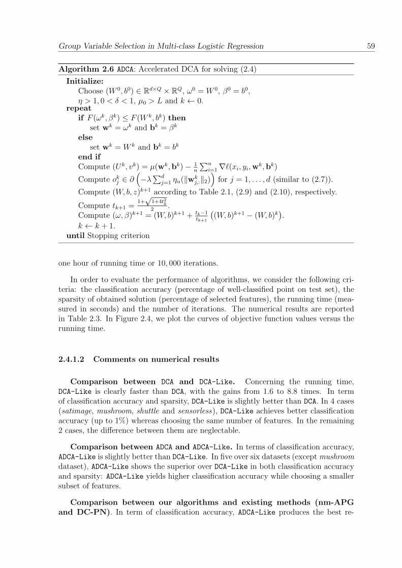
Group Variable Selection in Multi-class Logistic Regression 59
Algorithm 2.6 ADCA: Accelerated DCA for solving (2.4)
Initialize:Choose (W 0, b0) ∈ Rd×Q × RQ, ω0 = W 0, β0 = b0,η > 1, 0 < δ < 1, µ0 > L and k ← 0.
repeatif F (ωk, βk) ≤ F (W k, bk) then
set wk = ωk and bk = βk
elseset wk = W k and bk = bk
end ifCompute (Uk, vk) = µ(wk,bk)− 1
n
∑ni=1∇`(xi, yi,wk,bk)
Compute okj ∈ ∂(−λ∑d
j=1 ηα(‖wkj,:‖2)
)for j = 1, . . . , d (similar to (2.7)).
Compute (W, b, z)k+1 according to Table 2.1, (2.9) and (2.10), respectively.
Compute tk+1 =1+√
1+4t2k2
.Compute (ω, β)k+1 = (W, b)k+1 + tk−1
tk+1
((W, b)k+1 − (W, b)k
).
k ← k + 1.until Stopping criterion
one hour of running time or 10, 000 iterations.
In order to evaluate the performance of algorithms, we consider the following cri-teria: the classification accuracy (percentage of well-classified point on test set), thesparsity of obtained solution (percentage of selected features), the running time (mea-sured in seconds) and the number of iterations. The numerical results are reportedin Table 2.3. In Figure 2.4, we plot the curves of objective function values versus therunning time.
2.4.1.2 Comments on numerical results
Comparison between DCA and DCA-Like. Concerning the running time,DCA-Like is clearly faster than DCA, with the gains from 1.6 to 8.8 times. In termof classification accuracy and sparsity, DCA-Like is slightly better than DCA. In 4 cases(satimage, mushroom, shuttle and sensorless), DCA-Like achieves better classificationaccuracy (up to 1%) whereas choosing the same number of features. In the remaining2 cases, the difference between them are neglectable.
Comparison between ADCA and ADCA-Like. In terms of classification accuracy,ADCA-Like is slightly better than DCA-Like. In five over six datasets (except mushroomdataset), ADCA-Like shows the superior over DCA-Like in both classification accuracyand sparsity: ADCA-Like yields higher classification accuracy while choosing a smallersubset of features.
Comparison between our algorithms and existing methods (nm-APGand DC-PN). In term of classification accuracy, ADCA-Like produces the best re-

60 Group Variable Selection in Multi-class Logistic Regression
sults in all six datasets. As for the sparsity of solution, ADCA-Like also furnishesgood results: the best result on four datasets and the second-best result on the othertwo datasets. It is worth to mention that in two datasets (sensorless and shuttle),while most algorithms choose the same percentage of features, ADCA-Like has thehighest classification accuracy. We also observe that DC-PN often chooses the biggestsubset of features while giving lower classification accuracy. In term of computingtime, DCA-Like and ADCA-Like are arguably faster than the other algorithms, whereasnm-APG is the slowest. Overall, both ADCA-Like and ADCA achieve better results thannm-APG and DC-PN.
0 0.02 0.04 0.06 0.08
Time (seconds)
0.1
0.15
0.2
0.25
0.3
0.35
0.4
Obj
ectiv
e (lo
g-sc
ale)
DCAADCADCA-LikeADCA-LikenmAPGDC-PN
(a) dna
0 1 2 3 4 5 6
Time (seconds)
0.6
0.8
1
1.2
1.4
1.6
Obj
ectiv
e (lo
g-sc
ale)
DCAADCADCA-LikeADCA-LikenmAPGDC-PN
(b) satimage
0 0.01 0.02 0.03 0.04
Time (seconds)
0
0.05
0.1
0.15
0.2
0.25
Obj
ectiv
e (lo
g-sc
ale)
DCAADCADCA-LikeADCA-LikenmAPGDC-PN
(c) mushroom
0 0.005 0.01 0.015 0.02 0.025 0.03
Time (seconds)
0.05
0.1
0.15
0.2
0.25
Obj
ectiv
e (lo
g-sc
ale)
DCAADCADCA-LikeADCA-LikenmAPGDC-PN
(d) phishing
0 0.02 0.04 0.06
Time (seconds)
0.1
0.2
0.3
0.4
0.5
0.6
Obj
ectiv
e (lo
g-sc
ale)
DCAADCADCA-LikeADCA-LikenmAPGDC-PN
(e) shuttle
0 1 2 3
Time (seconds)
0.2
0.3
0.4
0.5
0.6
0.7
0.8
Obj
ectiv
e (lo
g-sc
ale)DCAADCADCA-LikeADCA-LikenmAPGDC-PN
(f) sensorless
Figure 2.4 – Objective value versus running time (average of ten runs)
2.5 Comparison between proposed algorithms
This section focuses on evaluating the performance of three proposed algorithms(SDCA, DCA-Like and ADCA-Like) for high-dimensional datasets.
Datasets: We performed numerical experiments on two types of data: realdatasets (CLL SUB 111, Carcinom, lung, ORL, BASEHOCK, protein and miniboone)and simulated datasets (sim 1 and sim 3 ). All real-world datasets are taken fromthe well-known UCI, LibSVM and Feature Selection Datasets 7 data repositories. Twosimulated datasets (sim 1 and sim 3 ) are generated from the same procedures in sec-tion 2.3.1.1.
Experiment setting Unless stated, this experiment’s settings are the same as insection 2.3.1. We employ grid search for λ ∈ 104, 3× 10³, 103, . . . , 3× 10⁻³, 10−3.
7. http://featureselection.asu.edu/datasets.php
[]

Group Variable Selection in Multi-class Logistic Regression 61
All experiments are performed on a PC Intel (R) i5-6300HQ CPU @2.30 GHz (4CPUs) with 8GB RAM.
The numerical experiment is reported in Table 2.4. We notice that:— The classification accuracy of DCA-Like and ADCA-Like are similar (< 0.1%
in 8 over 9 cases); and both are slightly higher than SDCA by up to 0.5% (inprotein and sim 1). Overall, the differences are neglectable.
— Similarly, in terms of sparsity, DCA-Like and ADCA-Like often choose the leastnumber of variables, and is much smaller than SDCA. The gap between DCA-Like
(reps. ADCA-Like) and SDCA is up to 9%, which is equivalent to 2 to 6 timesbigger subset of features in some datasets (CLL SUB 111, ORL and miniboone).
— In terms of running time, it is clear that SDCA is faster than DCA, especiallyfor large dataset. Except the three smallest datasets (CLL SUB 111, Carcinomand lung) where DCA-Like (reps. ADCA-Like) is faster than SDCA; SDCA isfaster. The reduction in running time is from 1.3 to 8 times; especially in thetwo biggest datasets where SDCA is faster than the second fastest ones by 4 and8 times respectively.
In conclusion, ADCA-Like is faster than DCA-Like, while having similar classifica-tion accuracy and sparsity. SDCA is much faster than ADCA-Like (reps. DCA-Like)while having similar accuracy; however ADCA-Like selects more compact subset ofvariables than SDCA.
2.6 Conclusion
We have rigorously studied the DC programming and DCA for the problem ofgroup variables selection in multi-class logistic regression. Using the `q,0 regularization,the resulting optimization problem is non-convex. The `q,0-norm is approximated bypiecewise exponential function and capped-`1 function. We have developed DCA-basedalgorithms to solve it by two approaches based on recent advanced DC algorithms.
The first approach developed an algorithm for multi-class logistic regression basedon Stochastic DCA. The proposed algorithm, SDCA, is very inexpensive and suitablefor large-scale datasets. SDCA exploits the special structure of the problem: not onlyall computation of SDCA are explicit, but SDCA also only requires a small subset of dataat each iteration for computing the subgradient of the second DC component, whichsignificantly reduces the running time. Numerical results showed that the proposedalgorithm reduces the running time of DCA (standard DCA for this problem) by morethan 19 times while achieving equivalent classification accuracy. Moreover, SDCA out-performs the two related algorithms (msgl and SPGD-`2,1): it reduces the running timeby more than 15 times while giving more accurate result. We are convinced that SDCAis fast and scalable method for the problem of group variable selection in multi-classlogistic regression.
In the second approach, we developed two algorithms for the multi-class logisticregression with group variables selection, DCA-Like and ADCA-Like. DCA-Like elimi-

62 Group Variable Selection in Multi-class Logistic Regression
nates the needs to compute µ, and iterative updating µ while keeping µ small, henceit potentially reduces the running time with better solution in compare with standardDCA. ADCA-Like improves DCA-Like by in-cooperating Nesterov’s acceleration. Bothalgorithms are efficient, all computation are explicit. DCA-Like and ADCA-Like im-proves the running time of DCA (by up to 8 times and 18.6 times respectively) whilehaving equivalent classification accuracy and sparsity. In addition, both of them de-liver better results than the two related algorithms (nm-APG and DC-PN) in both term ofclassification accuracy and running time. We can undoubtedly conclude that DCA-Likeand ADCA-Like improves DCA in this application.
In comparison between two proposed approaches, SDCA is more suitable for largedatasets as it is faster while achieving similar classification accuracy. In contrasts,ADCA-Like and DCA-Like is more suitable if we prefer a more compact subset ofvariables. And ADCA-Like is better than DCA-Like while achieving the similar clas-sification accuracy and sparsity. Hence, the choice for one method is depend on thecompactness of the solution and the size of the dataset. For small dataset, the suit-able choice is clearly ADCA-Like; whereas the choice for large dataset is based on thetrade-off between the compactness of the solution versus training time.
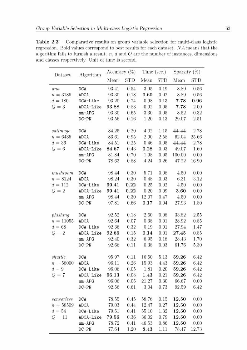
Group Variable Selection in Multi-class Logistic Regression 63
Table 2.3 – Comparative results on group variable selection for multi-class logisticregression. Bold values correspond to best results for each dataset. NA means that thealgorithm fails to furnish a result. n, d and Q are the number of instances, dimensionsand classes respectively. Unit of time is second.
Dataset AlgorithmAccuracy (%) Time (sec.) Sparsity (%)
Mean STD Mean STD Mean STD
dna DCA 93.41 0.54 3.95 0.19 8.89 0.56n = 3186 ADCA 93.30 0.18 0.60 0.02 8.89 0.56d = 180 DCA-Like 93.20 0.74 0.98 0.13 7.78 0.96Q = 3 ADCA-Like 93.88 0.83 0.92 0.05 7.78 2.00
nm-APG 93.30 0.65 3.30 0.05 8.52 0.32DC-PN 93.56 0.16 1.20 0.13 29.07 2.51
satimage DCA 84.25 0.20 4.02 1.15 44.44 2.78n = 6435 ADCA 83.61 0.95 2.90 2.58 62.04 25.66d = 36 DCA-Like 84.51 0.25 0.46 0.05 44.44 2.78Q = 6 ADCA-Like 84.67 0.43 0.28 0.03 49.07 1.60
nm-APG 81.84 0.70 1.98 0.05 100.00 0.00DC-PN 78.63 0.88 4.24 0.26 47.22 16.90
mushroom DCA 98.44 0.30 5.71 0.08 4.50 0.00n = 8124 ADCA 98.24 0.30 0.48 0.03 6.31 3.12d = 112 DCA-Like 99.41 0.22 0.25 0.02 4.50 0.00Q = 2 ADCA-Like 99.41 0.22 0.20 0.09 3.60 0.00
nm-APG 98.44 0.30 12.07 0.47 4.50 0.00DC-PN 97.81 0.66 0.17 0.04 27.93 1.80
phishing DCA 92.52 0.18 2.60 0.08 33.82 2.55n = 11055 ADCA 92.64 0.07 0.38 0.01 28.92 0.85d = 68 DCA-Like 92.36 0.32 0.19 0.01 27.94 1.47Q = 2 ADCA-Like 92.66 0.15 0.14 0.01 27.45 0.85
nm-APG 92.40 0.32 6.95 0.18 28.43 1.70DC-PN 92.66 0.11 0.38 0.03 61.76 5.30
shuttle DCA 95.97 0.11 16.50 5.13 59.26 6.42n = 58000 ADCA 96.11 0.26 15.93 4.43 59.26 6.42d = 9 DCA-Like 96.06 0.05 1.81 0.20 59.26 6.42Q = 7 ADCA-Like 96.13 0.08 1.43 0.21 59.26 6.42
nm-APG 96.06 0.05 21.27 0.30 66.67 0.00DC-PN 92.56 0.61 3.04 0.73 92.59 6.42
sensorless DCA 78.55 0.45 58.76 0.15 12.50 0.00n = 58509 ADCA 79.03 0.44 12.47 0.27 12.50 0.00d = 54 DCA-Like 79.51 0.41 55.10 1.32 12.50 0.00Q = 11 ADCA-Like 79.56 0.36 36.02 0.79 12.50 0.00
nm-APG 78.72 0.41 46.53 0.86 12.50 0.00DC-PN 77.64 1.20 8.43 1.11 78.47 12.73

64 Group Variable Selection in Multi-class Logistic Regression
Table 2.4 – Comparative results on group variable selection for multi-class logisticregression. Bold values correspond to best results for each dataset. NA means that thealgorithm fails to furnish a result. n, d and Q are the number of instances, dimensionsand classes respectively. Unit of time is second.
Dataset AlgorithmAccuracy (%) Time (sec.) Sparsity (%)
Mean STD Mean STD Mean STD
CLL SUB 111 DCA-Like 78.79 6.94 0.75 0.03 0.32 0.18n× d = 111× 11340 ADCA-Like 78.79 6.94 0.63 0.06 0.18 0.04Q = 3 SDCA 78.79 5.25 5.25 1.64 1.95 1.09
Carcinom DCA-Like 89.52 8.25 3.06 0.05 0.41 0.01n× d = 174× 9182 ADCA-Like 90.48 6.60 1.81 0.11 0.41 0.01Q = 11 SDCA 90.48 6.60 4.16 2.74 0.66 0.25
lung DCA-Like 91.06 3.73 0.71 0.01 0.47 0.02n× d = 203× 3312 ADCA-Like 91.06 3.73 0.42 0.08 0.50 0.02Q = 5 SDCA 91.06 3.73 0.86 0.10 0.57 0.11
ORL DCA-Like 94.58 5.05 10.76 0.56 6.02 0.31n× d = 400× 1024 ADCA-Like 94.58 2.89 7.43 0.76 7.71 0.34Q = 40 SDCA 94.58 5.05 3.04 1.38 16.76 6.69
BASEHOCK DCA-Like 94.65 1.26 5.72 2.53 4.24 0.87n× d = 1993× 4862 ADCA-Like 94.65 1.38 5.47 1.51 2.28 0.69Q = 2 SDCA 94.74 0.25 3.54 0.28 2.73 0.16
protein DCA-Like 68.26 0.50 2.92 0.43 77.90 2.03n× d = 24387× 357 ADCA-Like 68.29 0.51 4.16 0.90 78.00 2.13Q = 3 SDCA 67.94 0.62 1.17 0.35 80.43 0.58
sim 1 DCA-Like 72.22 0.50 0.66 0.00 80.00 0.00n× d = 100000× 50 ADCA-Like 72.22 0.50 0.63 0.02 80.00 0.00Q = 4 SDCA 72.18 0.57 0.49 0.06 80.00 0.00
miniboone DCA-Like 83.78 0.07 4.82 0.42 6.00 0.00n× d = 130064× 50 ADCA-Like 83.78 0.07 3.68 0.60 6.00 0.00Q = 2 SDCA 84.25 0.34 0.92 0.23 11.33 1.15
sim 3 DCA-Like 99.93 0.01 358.40 7.38 80.00 0.00n× d = 250000× 500 ADCA-Like 99.93 0.01 159.95 16.26 80.00 0.00Q = 4 SDCA 99.93 0.02 17.86 3.28 80.00 0.00
Chapter 3
t-distributed Stochastic NeighborEmbedding 1
Abstract: t-distributed Stochastic Neighbor Embedding (t-SNE) is a popular method for dimen-sional reduction and data visualization, especially for high-dimensional data. In this chapter,we developed two alogrithms based on advanced DCAs – DCA-Like and ADCA-Like – for thet-SNE problem. DCA-Like relaxes the convexity condition of the second DC component whileensuring the convergence; whereas ADCA-Like in-cooperates the Nesterov’s acceleration tech-nique into DCA-Like, which potentially leads to better solution in comparison to DCA-Like.It turns out that Majorization Minimization, the best state-of-the-art algorithm for t-SNE,is DCA-Like applied for t-SNE. Numerical experiments on several benchmark datasets forvisualizing high-dimensional data illustrate the efficiency of our algorithms.
1. The material of this chapter is developed from the following work:[1] H.A. Le Thi, H.M. Le, D.N. Phan, B. Tran. Novel DCA Based Algorithms for Minimizing the Sumof a Nonconvex Function and Composite Functions with Applications in Machine learning. Submitted& Available on arvXiv [arXiv:1806.09620].
65

66 t-distributed Stochastic Neighbor Embedding
3.1 Introduction
Dimensional reduction for high-dimensional data, especially in data visualization,is an important task in data mining. Due to the nature of high-dimensional data whereonly pairwise distances are reliable, many techniques exploit this property by tryingto preserve the small pairwise distance in low-dimensional embedding. Among them,t-SNE is a gaining popular method from the family of stochastic neighbor embedding(SNE) methods [34], operates by retaining local pairwise distances. t-SNE was firstintroduced in [106] as a visualization technique for high dimensional data. Later, ithas been applied in many applications such as bioinformatic [114], cancer research,visualize features in neural networks [77], etc.
The t-SNE problem is formulated as the minimization of the divergence betweentwo distributions: (1) a distribution that measures pairwise similarities of the inputobjects and (2) a distribution that measures pairwise similarities of the correspondinglow-dimensional points in the embedding. This problem is described as follows. Givena data set of n objects D = a1, ..., an with ai ∈ Rd, t-SNE aims to find their low-dimensional representation E = x1, ...,xn with xi ∈ Rs (d s) which preserves thepairwise similarities of input objects. To this end, t-SNE defines joint probabilities pijthat measure the pairwise similarity between objects xi and xj by symmetrizing two
conditional probabilities as pij =pj|i+pi|j
2n, where
pj|i =
exp(−‖ai−aj‖2/2σ2
i )∑k 6=i exp(−‖ai−ak‖2/2σ2
i )if i 6= j,
0 otherwise.
In the embedding subspace E , the similarities between two points xi and xj aremeasured using a normalized heavy-tailed kernel. Specifically, the embedding similar-ity qij between the two points xi and xj is computed as a normalized Student-t kernelwith a single degree of freedom:
qij =
(1+‖xi−xj‖2)−1∑k 6=l(1+‖xk−xl‖2)−1 if i 6= j,
0 otherwise.
The locations of the embedding points xi are determined by minimizing theKullback-Leibler divergence between the joint distributions P and Q:
minx
KL(P ||Q) =
∑i6=j
pij logpijqij
, (3.1)
which is equivalent to
minx
F (x) = f(x) +
∑i,j
pij log(1 + ‖xi − xj‖2)
, (3.2)
where f(x) = log(∑
i6=j(1 + ‖xi − xj‖2)−1).
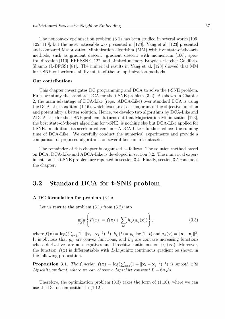
t-distributed Stochastic Neighbor Embedding 67
The nonconvex optimization problem (3.1) has been studied in several works [106,122, 110], but the most noticeable was presented in [123]. Yang et al. [123] presentedand compared Majorization Minimization algorithm (MM) with five state-of-the-artsmethods, such as gradient descent, gradient descent with momentum [106], spec-tral direction [110], FPHSSNE [122] and Limited-memory Broyden-Fletcher-Goldfarb-Shanno (L-BFGS) [81]. The numerical results in Yang et al. [123] showed that MMfor t-SNE outperforms all five state-of-the-art optimization methods.
Our contributions
This chapter investigates DC programming and DCA to solve the t-SNE problem.First, we study the standard DCA for the t-SNE problem (3.2). As shown in Chapter2, the main advantage of DCA-Like (reps. ADCA-Like) over standard DCA is usingthe DCA-Like condition (1.16), which leads to closer majorant of the objective functionand potentiality a better solution. Hence, we develop two algorithms by DCA-Like andADCA-Like for the t-SNE problem. It turns out that Majorization Minimization [123],the best state-of-the-art algorithm for t-SNE, is nothing else but DCA-Like applied fort-SNE. In addition, its accelerated version – ADCA-Like – further reduces the runningtime of DCA-Like. We carefully conduct the numerical experiments and provide acomparison of proposed algorithms on several benchmark datasets.
The remainder of this chapter is organized as follows. The solution method basedon DCA, DCA-Like and ADCA-Like is developed in section 3.2. The numerical exper-iments on the t-SNE problem are reported in section 3.4. Finally, section 3.5 concludesthe chapter.
3.2 Standard DCA for t-SNE problem
A DC formulation for problem (3.1):
Let us rewrite the problem (3.1) from (3.2) into
minx∈X
F (x) := f(x) +
∑i,j
hij(gij(x))
, (3.3)
where f(x) = log(∑
i6=j(1+‖xi−xj‖2)−1), hij(t) = pij log(1+t) and gij(x) = ‖xi−xj‖2.It is obvious that gij are convex functions, and hij are concave increasing functionswhose derivatives are non-negatives and Lipschitz continuous on [0,+∞). Moreover,the function f(x) is differentiable with L-Lipschitz continuous gradient as shown inthe following proposition.
Proposition 3.1. The function f(x) = log(∑
i6=j(1 + ‖xi − xj‖2)−1) is smooth with
Lipschitz gradient, where we can choose a Lipschitz constant L = 6n√s.
Therefore, the optimization problem (3.3) takes the form of (1.10), where we canuse the DC decomposition in (1.12).

68 t-distributed Stochastic Neighbor Embedding
DCA scheme for problem (3.1):
Since the optimization problem (3.3) takes the form of (1.10), then according toDCA scheme (1.2), at each iteration, we have to compute
ξkij = ∇(−hij)(gij(xki ,xkj )) = − pij1 + ‖xki − xkj‖2
and ∇f(xk) by
∇xif(xk) =n∑j=1
−4(xki − xkj )(1 + ‖xki − xkj‖2)−2∑l 6=m(1 + ‖xkl − xkm‖2)−1
, (3.4)
and solve the following convex problem to compute xk+1
minx
µk2‖x− xk‖2 + 〈∇f(xk),x〉+
∑i,j
−ξkij‖xi − xj‖2
.
The solution xk+1 of the above problem is given by
xk+1 = (2L−ξk−(ξk)T + µkI)−1(−∇f(xk) + µkxk), (3.5)
where the matrix ξk is defined by the elements ξkij and LA denotes the matrix with(LA)ij = −Aij if i 6= j and −Aii +
∑nl=1 Ail otherwise.
The standard DCA for solving the t-SNE problem (3.1) is presented in Algorithm3.1.
Algorithm 3.1 DCA: DCA for solving t-SNE problem (3.1)
Initialize:Choose x0, µ0 > L and k ← 0.
repeatCompute ξkij = − pij
1+‖xki−xkj ‖2and ∇f(xk) by (3.4).
Compute xk+1 by (3.5).k ← k + 1.
until Stopping condition
3.3 DCA-Like and ADCA-Like for t-SNE problem
The DCA (Algorithm 3.1) requires setting µ0 ≥ L, where we have estimatedL = 6n
√s. This value is clearly too large, which could lead to a bad convex ap-
proximation of F , then potentially a bad solution. Hence, we consider DCA-Like tosolve this problem. As we have mentioned in Section 1.3.2, the goal of DCA-Like isto avoid bad approximations of the objective function with a too large value of µ (c.f.

t-distributed Stochastic Neighbor Embedding 69
Algorithm 1.2). The main idea of DCA-Like is to keep the parameter µ as small aspossible while finding a convex approximation of objecive function. By using a smallvalue of µk, we can get a closer majorant of the objective function which could lead toa better solution. According to the Algorithm 1.3, stops if the following inequalityholds
Utsneµk
(xk+1,xk) ≥ F (xk+1), (3.6)
where Utsneµk
(xk+1,xk) = F (xk)+〈∇f(xk),xk+1−xk〉+ µk2‖xk+1−xk‖2−〈ξk, g(xk+1)−
g(xk)〉. From the update rule (3.5) for xk+1 and this stopping criterion for searching µk,we can conclude that MM [123] for (3.1) is a special version of DCA-Like. DCA-Likefor solving t-SNE problem (3.1) is described in Algorithm 3.2.
Algorithm 3.2 DCA-Like: DCA-Like for solving t-SNE problem (3.1)
Initialize:Choose x0, η > 1, 0 < δ < 1, µ0 > 0 and k ← 0.
repeatCompute ξkij = − pij
1+‖xki−xkj ‖2and ∇f(xk) by (3.4).
Set µk = maxµ0, δµk−1 if k > 0.Compute xk+1 by (3.5).while Utsne
µk(xk+1,xk) < F (xk+1) do
µk ← ηµk.Compute xk+1 by (3.5).
end whilek ← k + 1.
until Stopping criterion
ADCA-Like for solving (3.1) is obtained by adding the acceleration steps of Algo-rithm 1.4 to Algorithm 3.2, and is presented in Algorithm 3.3.
3.4 Numerical experiment
Experiment setting
To evaluate the performances of our methods, we perform numerical experimentson 13 datasets taken from UCI data repository 2 and Feature Selection repository 3.20news and rcv1 dataset are downloaded and pre-processed using the same detailedprocedure in [26, 117].
The comparison is realized on three criteria: the objective value F (x), the numberof iterations and the computation time (measured in seconds). Each experiment isrepeated 10 times, then the final result is the average value of each criterion. Theresults are reported in the Table 3.1.
2. http://archive.ics.uci.edu/ml/index.php
3. http://featureselection.asu.edu/datasets.php

70 t-distributed Stochastic Neighbor Embedding
Algorithm 3.3 ADCA-Like: Accelerated DCA-Like for solving t-SNE problem (3.1)
Initialize:Choose x0, w0 = x0, η > 1, 0 < δ < 1, µ0 > 0 and k ← 0.
repeatif F (wk) ≤ F (xk) then
set vk = wk;else
set vk = xk.end ifCompute ξkij = − pij
1+‖vki −vkj ‖2and ∇f(vk) by (3.4).
Set µk = maxµ0, δµk−1 if k > 0.Compute xk+1 by (3.5).while Utsne
µk(xk+1,xk) < F (xk+1) do
µk ← ηµk.Compute xk+1 by (3.5).
end while
Compute tk+1 =1+√
1+4t2k2
.Compute wk+1 = xk+1 + tk−1
tk+1
(xk+1 − xk
).
k ← k + 1.until Stopping criterion
Algorithm 3.4 ADCA: Accelerated DCA for solving t-SNE problem (3.1)
Initialize:Choose x0, w0 = x0, η > 1, 0 < δ < 1, µ0 > L and k ← 0.
repeatif F (wk) ≤ F (xk) then
set vk = wk;else
set vk = xk.end ifCompute ξkij = − pij
1+‖vki −vkj ‖2and ∇f(vk) by (3.4).
Compute xk+1 by (3.5).
Compute tk+1 =1+√
1+4t2k2
.Compute wk+1 = xk+1 + tk−1
tk+1
(xk+1 − xk
).
k ← k + 1.until Stopping criterion
The comparisons are performed between 5 algorithms: DCA, DCA-Like, ADCA,ADCA-Like and DC-PN (DC Proximal Newton [91]). DC-PN is a DCA-based algorithmfor minimizing f(x) + h(x), where f(x) = f1(x)− f2(x) is a DC function, twice differ-entiable, with f(x) verifying the L-Lipschitz gradient property; h(x) = h1(x) − h2(x)where both h1 and h2 are convex functions and (possibly) non-differential. Notethat, in DC-PN, L-BFGS is employed for approximating the Hessian matrix Hk; and

t-distributed Stochastic Neighbor Embedding 71
the sub-problem is solved by minFunc solver 4. ADCA, the accelerate version of Algo-rithm 3.1 [89], is described in Algorithm 3.4.
As mentioned before, in the DCA (Algorithm 3.1) and ADCA (Algorithm 3.4), wehave to estimate the L-Lipschitz constant of f . According to Proposition 3.1, we canchoose L = 6n
√s. This value is clearly too large. Hence, we incorporate a µ updating
procedure into DCA and ADCA. We start with a small value of µ and increase µ if theobjective value increases in DCA/ADCA scheme. For all algorithms, the initial value ofµ is set to be µ0 = 10−6.
Stopping conditions of all algorithms are the same, by either (1) number of itera-tions exceeds 10, 000 or (2) ‖xk − xk−1‖/‖xk−1‖ ≤ 10−8. Throughout our experiment,the number of embedding dimension is set to s = 2. All experiments are performedon a PC Intel (R) Xeon (R) E5-2630 v4 @2.20 GHz of 32GB RAM.
For large datasets, Barnes-Hut tree approximation is used for reducing computingcost [74]. This technique is well-known in Neighbor Embedding problems, which pro-vides a good trade-off small loss in gradients and cost function against huge reductionin computation time. We set the parameter θBarnes-Hut = 0.5.
We adopt the same test process as described in [123]. For all datasets, k-NearestNeighbor (with k = 10) is employed to construct pij, where pij = 1 if data point j (reps.i) is one of k nearest neighbors of data point j (reps. i), and pij = 0 otherwise. pij isthen computed by pij =
pij∑k,l pkl
. The initial point x0 is drawn from normal distribution
N (0, 10−8) for all methods. Early exaggeration technique [106] is deployed for first 20iterations with the constant value of 4.
Table 3.1 – Comparative results on datasets. Bold values correspond to best resultsfor each dataset, n and d are the number of instances and dimensions respectively.Unit of time is second.
Dataset AlgorithmObjective Iteration Time (sec.)
Mean STD Mean STD Mean STD
tox 171 DCA 1.52 0.03 22 0 0.64 0.01n = 171 ADCA 1.62 0.64 37 22 1.95 1.38d = 5748 DCA-Like (MM) 1.25 0.00 46 3 2.92 0.21
ADCA-Like 1.25 0.00 49 21 3.54 1.40DC-PN 1.25 0.00 83 5 0.62 0.04
orl DCA 1.86 0.20 23 2 5.50 4.77n = 400 ADCA 1.59 0.00 59 23 15.10 3.59d = 1024 DCA-Like (MM) 1.59 0.00 54 13 17.45 3.49
ADCA-Like 1.59 0.01 68 30 20.43 8.18DC-PN 1.62 0.01 177 47 3.25 0.82
4. minFunc: unconstrained differentiable multivariate optimization in Matlab. http://www.cs.
ubc.ca/~schmidtm/Software/minFunc.html

72 t-distributed Stochastic Neighbor Embedding
relathe DCA 3.82 0.00 22 0 2.98 0.04n = 1427 ADCA 3.05 0.02 61 23 18.69 7.09d = 4322 DCA-Like (MM) 3.03 0.01 71 15 26.74 9.86
ADCA-Like 3.02 0.00 67 2 28.85 1.98DC-PN 3.10 0.04 1,044 313 117.36 32.09
pcmac DCA 4.35 0.00 22 0 1.87 0.07n = 1943 ADCA 3.60 0.01 103 10 11.10 0.45d = 3289 DCA-Like (MM) 3.59 0.00 103 11 14.88 1.07
ADCA-Like 3.59 0.01 81 16 13.78 2.67DC-PN 3.69 0.01 1,363 124 232.60 39.44
gisette DCA 3.52 0.04 27 0 15.3 0.2n = 7000 ADCA 3.33 0.00 118 31 39.5 7.9d = 5000 DCA-Like (MM) 3.34 0.01 283 81 209.0 57.9
ADCA-Like 3.32 0.02 133 24 62.9 10.0DC-PN 3.53 0.02 2187 186 1218.3 194.3
usps DCA 2.41 0.01 29 1 23.1 1.8n = 9298 ADCA 3.92 1.36 70 107 27.9 39.0d = 256 DCA-Like (MM) 2.34 0.00 106 18 62.5 11.0
ADCA-Like 2.34 0.01 107 15 64.9 6.0DC-PN 2.57 0.07 2083 538 1315.2 171.7
rcv1 DCA 5.39 0.41 30 13 17.43 10.31n = 10000 ADCA 4.86 0.05 259 179 119.11 57.89d = 2000 DCA-Like (MM) 4.84 0.00 295 88 135.77 45.39
ADCA-Like 4.82 0.00 130 22 78.53 20.99DC-PN 5.13 0.03 5,083 582 9,783.73 2,539.40
20news DCA 3.67 0.05 78 27 160.57 84.05n = 18846 ADCA 3.64 0.09 221 145 207.45 114.95d = 2000 DCA-Like (MM) 3.45 0.01 687 147 1,378.75 353.95
ADCA-Like 3.43 0.01 145 5 208.51 8.62DC-PN 3.93 0.02 3,156 79 6,843.18 280.67
magic DCA 2.40 0.00 850 373 413.4 170.4n = 19020 ADCA 2.46 0.01 215 9 150.5 9.8d = 10 DCA-Like (MM) 2.36 0.00 168 39 135.2 31.1
ADCA-Like 2.36 0.00 106 7 101.7 4.8DC-PN 2.80 0.07 3498 237 4321.0 557.8
letters DCA 1.58 0.02 1186 159 652.8 98.2n = 20000 ADCA 1.49 0.02 369 104 268.4 86.8d = 16 DCA-Like (MM) 1.48 0.01 164 24 149.0 19.3
ADCA-Like 1.48 0.01 90 7 96.8 7.4

t-distributed Stochastic Neighbor Embedding 73
DC-PN 2.14 0.07 1326 253 1997.1 539.0
shuttle DCA 1.60 0.02 3520 459 6056.5 782.9n = 58000 ADCA 1.48 0.04 760 96 1781.7 215.1d = 9 DCA-Like (MM) 1.45 0.02 333 9 981.7 33.1
ADCA-Like 1.42 0.00 152 23 553.7 123.6DC-PN 2.54 0.03 4693 68 26784.4 3633.2
sensorless DCA 3.18 0.02 1788 454 3232.1 837.3n = 58509 ADCA 3.13 0.01 418 24 912.8 50.0d = 48 DCA-Like (MM) 3.21 0.02 313 41 953.7 114.5
ADCA-Like 3.18 0.02 153 28 499.3 91.2DC-PN 3.81 0.04 4255 144 20586.9 4488.6
mnist DCA 3.44 0.00 3894 111 13752.7 644.9n = 70000 ADCA 3.45 0.01 960 60 2659.1 63.3d = 784 DCA-Like (MM) 3.46 0.01 371 67 1576.8 259.7
ADCA-Like 3.43 0.01 196 27 834.1 127.5DC-PN 4.12 0.01 3703 308 21486.7 3643.1
miniboone DCA 3.55 0.05 3401 1151 20473.3 6471.2n = 130064 ADCA 3.47 0.06 454 338 2917.1 2050.2d = 50 DCA-Like (MM) 3.53 0.05 469 61 4841.7 691.5
ADCA-Like 3.53 0.02 170 12 1560.6 209.1DC-PN 5.36 0.15 471 29 7071.7 844.0
covertype DCA 2.14 0.00 3998 35 71591.8 1407.2n = 581012 ADCA 1.88 0.00 1670 0 29954.8 0.0d = 54 DCA-Like (MM) 2.10 0.04 1217 66 37123.1 3546.5
ADCA-Like 1.68 0.01 330 10 8338.4 191.8DC-PN 4.24 0.00 5741 45 140122.8 5126.4
Comments on numerical results— We first interest in the performance of DCA-Like in compare to DCA. It is clear
that DCA-Like is better than DCA. DCA-Like gives a lower or equal objectivevalue than DCA in 13 out of 15 datasets (all except sensorless and mnist). Fordataset with more than 19, 000 datapoints, the running time of DCA-Like isfrom 1.9 to 8.7 times less than DCA. For other cases, although DCA is faster thanDCA-Like, the objective value of DCA higher than than DCA-Like by a largemargin.
— We study now the benefit of using acceleration technique. The comparison ismade between 2 pairs: ADCA versus DCA and ADCA-Like versus DCA-Like. Aswe can see, ADCA-Like improves the performance of DCA-Like. The gains incomputing time are huge, as ADCA-Like is faster than DCA-Like from 1.0 to 6.6times (for datasets with more than 1000 datapoints, the reset are neglectable).
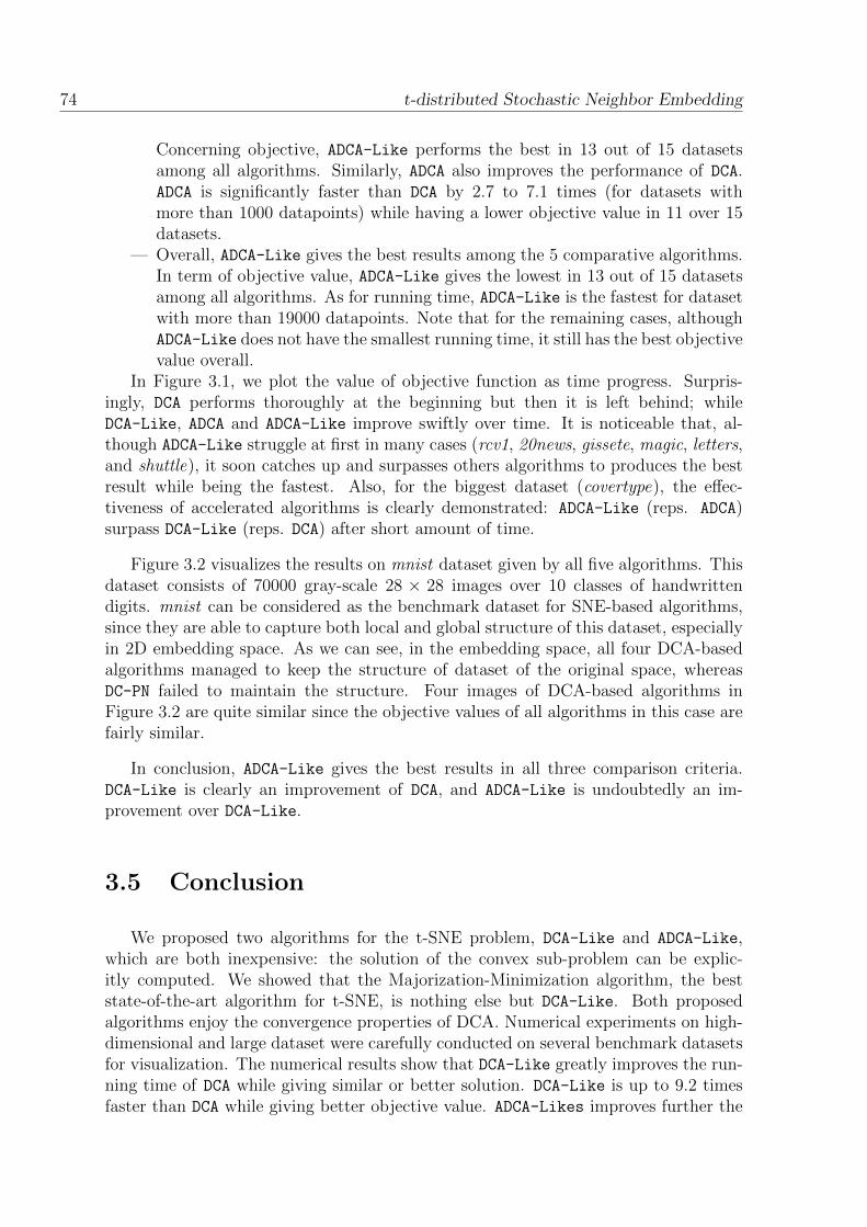
74 t-distributed Stochastic Neighbor Embedding
Concerning objective, ADCA-Like performs the best in 13 out of 15 datasetsamong all algorithms. Similarly, ADCA also improves the performance of DCA.ADCA is significantly faster than DCA by 2.7 to 7.1 times (for datasets withmore than 1000 datapoints) while having a lower objective value in 11 over 15datasets.
— Overall, ADCA-Like gives the best results among the 5 comparative algorithms.In term of objective value, ADCA-Like gives the lowest in 13 out of 15 datasetsamong all algorithms. As for running time, ADCA-Like is the fastest for datasetwith more than 19000 datapoints. Note that for the remaining cases, althoughADCA-Like does not have the smallest running time, it still has the best objectivevalue overall.
In Figure 3.1, we plot the value of objective function as time progress. Surpris-ingly, DCA performs thoroughly at the beginning but then it is left behind; whileDCA-Like, ADCA and ADCA-Like improve swiftly over time. It is noticeable that, al-though ADCA-Like struggle at first in many cases (rcv1, 20news, gissete, magic, letters,and shuttle), it soon catches up and surpasses others algorithms to produces the bestresult while being the fastest. Also, for the biggest dataset (covertype), the effec-tiveness of accelerated algorithms is clearly demonstrated: ADCA-Like (reps. ADCA)surpass DCA-Like (reps. DCA) after short amount of time.
Figure 3.2 visualizes the results on mnist dataset given by all five algorithms. Thisdataset consists of 70000 gray-scale 28 × 28 images over 10 classes of handwrittendigits. mnist can be considered as the benchmark dataset for SNE-based algorithms,since they are able to capture both local and global structure of this dataset, especiallyin 2D embedding space. As we can see, in the embedding space, all four DCA-basedalgorithms managed to keep the structure of dataset of the original space, whereasDC-PN failed to maintain the structure. Four images of DCA-based algorithms inFigure 3.2 are quite similar since the objective values of all algorithms in this case arefairly similar.
In conclusion, ADCA-Like gives the best results in all three comparison criteria.DCA-Like is clearly an improvement of DCA, and ADCA-Like is undoubtedly an im-provement over DCA-Like.
3.5 Conclusion
We proposed two algorithms for the t-SNE problem, DCA-Like and ADCA-Like,which are both inexpensive: the solution of the convex sub-problem can be explic-itly computed. We showed that the Majorization-Minimization algorithm, the beststate-of-the-art algorithm for t-SNE, is nothing else but DCA-Like. Both proposedalgorithms enjoy the convergence properties of DCA. Numerical experiments on high-dimensional and large dataset were carefully conducted on several benchmark datasetsfor visualization. The numerical results show that DCA-Like greatly improves the run-ning time of DCA while giving similar or better solution. DCA-Like is up to 9.2 timesfaster than DCA while giving better objective value. ADCA-Likes improves further the

t-distributed Stochastic Neighbor Embedding 75
running time (by up to 5 times) as well as the objective value of DCA-Like. Thus, wecan undoubtedly conclude the two proposed method, DCA-Like and ADCA-Like, arethe state-of-the-art algorithms for solving the t-SNE problem.
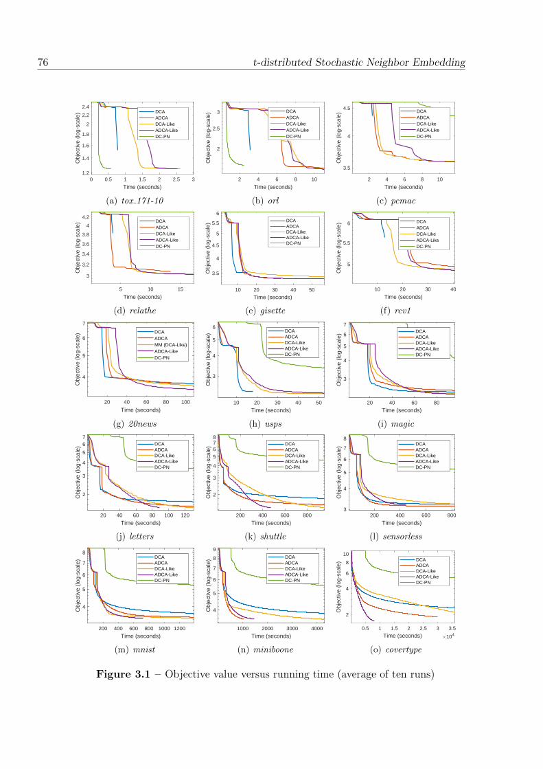
76 t-distributed Stochastic Neighbor Embedding
0 0.5 1 1.5 2 2.5 3
Time (seconds)
1.2
1.4
1.6
1.8
2
2.2
2.4
Obj
ectiv
e (lo
g-sc
ale)
DCAADCADCA-LikeADCA-LikeDC-PN
(a) tox 171-10
2 4 6 8 10
Time (seconds)
2
2.5
3
Obj
ectiv
e (lo
g-sc
ale)
DCAADCADCA-LikeADCA-LikeDC-PN
(b) orl
2 4 6 8 10
Time (seconds)
3.5
4
4.5
Obj
ectiv
e (lo
g-sc
ale)
DCAADCADCA-LikeADCA-LikeDC-PN
(c) pcmac
5 10 15
Time (seconds)
3
3.2
3.4
3.6
3.8
4
4.2
Obj
ectiv
e (lo
g-sc
ale)
DCAADCADCA-LikeADCA-LikeDC-PN
(d) relathe
10 20 30 40 50
Time (seconds)
3.5
4
4.5
5
5.5
6O
bjec
tive
(log-
scal
e)
DCAADCADCA-LikeADCA-LikeDC-PN
(e) gisette
10 20 30 40
Time (seconds)
5
5.5
6
Obj
ectiv
e (lo
g-sc
ale)
DCAADCADCA-LikeADCA-LikeDC-PN
(f) rcv1
20 40 60 80 100
Time (seconds)
4
5
6
7
Obj
ectiv
e (lo
g-sc
ale)
DCAADCAMM (DCA-Like)ADCA-LikeDC-PN
(g) 20news
10 20 30 40 50
Time (seconds)
3
4
5
6
Obj
ectiv
e (lo
g-sc
ale)
DCAADCADCA-LikeADCA-LikeDC-PN
(h) usps
20 40 60 80
Time (seconds)
3
4
5
6
7
Obj
ectiv
e (lo
g-sc
ale)
DCAADCADCA-LikeADCA-LikeDC-PN
(i) magic
20 40 60 80 100 120
Time (seconds)
2
3
4
5
67
Obj
ectiv
e (lo
g-sc
ale)
DCAADCADCA-LikeADCA-LikeDC-PN
(j) letters
200 400 600 800
Time (seconds)
2
3
4
5678
Obj
ectiv
e (lo
g-sc
ale)
DCAADCADCA-LikeADCA-LikeDC-PN
(k) shuttle
200 400 600 800
Time (seconds)
3
4
5
6
7
8
Obj
ectiv
e (lo
g-sc
ale)
DCAADCADCA-LikeADCA-LikeDC-PN
(l) sensorless
200 400 600 800 1000 1200
Time (seconds)
4
5
6
7
8
Obj
ectiv
e (lo
g-sc
ale)
DCAADCADCA-LikeADCA-LikeDC-PN
(m) mnist
1000 2000 3000 4000
Time (seconds)
4
5
6
7
8
9
Obj
ectiv
e (lo
g-sc
ale)
DCAADCADCA-LikeADCA-LikeDC-PN
(n) miniboone
0.5 1 1.5 2 2.5 3 3.5
Time (seconds) 104
2
4
6
8
10
Obj
ectiv
e (lo
g-sc
ale)
DCAADCADCA-LikeADCA-LikeDC-PN
(o) covertype
Figure 3.1 – Objective value versus running time (average of ten runs)
\ E \ I'\
D
X

t-distributed Stochastic Neighbor Embedding 77
(a) DCA (b) ADCA
(c) DCA-Like (d) ADCA-Like
(e) DC-PN
Figure 3.2 – Visualization of embedding space on mnist dataset. Colors representclasses of data (0 – 9).


Chapter 4
Deep Clustering1
Abstract: In this chapter, we propose new approaches for clustering high-dimensional data.The first approach considers the usage of t-SNE (t-Distributed Stochastic Neighbor Embed-ding) in clustering. We propose two clustering algorithms based on DC Programming andDCA. In the second approach, we consider the problem of joint-clustering using auto-encoder.We propose an extension by using a scale invariance distance measures for a class of joint-clustering problem using auto-encoder, and apply for a particular case of joint-clustering withMSSC (minimizing sum-of-square clustering). The efficiency of the proposed algorithms incomparison with the state-of-the-art algorithms on real-world high-dimensional datasets areempirically demonstrated in terms of clustering quality and running time.
1. The material of this chapter is developed from the following works:[1] H.A. Le Thi, B. Tran. A DCA-based approach for Joint Clustering and Dimensional Reduction byt-SNE. Submitted.[2] B. Tran, H.A. Le Thi. Deep Clustering with Spherical Distance in Latent Space. In: AdvancedComputational Methods for Knowledge Engineering. ICCSAMA 2019. Advances in Intelligent Sys-tems and Computing, Springer, Cham. Accepted.[3] G. Da Silva, H.M. Le, H.A. Le Thi, V. Lefieux, B. Tran. Customer Clustering of French Trans-mission System Operator (RTE) Based on Their Electricity Consumption. In: Le Thi H., Le H.,Pham Dinh T. (eds) Optimization of Complex Systems: Theory, Models, Algorithms and Applica-tions. WCGO 2019. Advances in Intelligent Systems and Computing, vol 991, pp. 893–905. Springer,Cham.
79
80 Deep Clustering
4.1 Introduction and related works
Clustering is an important task in data mining with the aim of segmenting data-points into groups which pose similarity. Despite decades of research, clustering high-dimensional datasets is still a difficult problem due to the “curse of dimensionality”phenomenon. In general terms, it is “the widely observed phenomenon that dataanalysis techniques (including clustering), which work well at lower dimensions, of-ten perform poorly as the dimensionality of analyzed data increases” [101]. Usingdimension reduction techniques is a popular way to overcome this problem, where theoriginal features are presented by a smaller but informative set of features. For cluster-ing methods using dimensional reduction techniques, we can categorize them by twocomponents: clustering approaches and dimensionality reduction methods.
There are two main approaches of using dimensional reduction techniques in clus-tering: “tandem analysis” approach (or two-step approach) and joint-clustering ap-proach. The first approach, “tandem analysis”, first introduced in [7], refers to aclustering procedure of two steps. The first step transforms the high-dimensional datato a lower-dimensional space (embedding space) that has preferable properties, wherea clustering algorithm is performed on such space in the second step. This approachhas extensively studied in the literature and has proved to be effective (better clus-tering results), such as Principal Component Analysis (PCA) [16, 128], Non-negativeMatrix Factorization (NMF) [118], Volume Minimization-based Factorization [119],Auto-encoder, Isomap [124, 132], etc. However, since these two steps are applied sepa-rately, the obtained embedding data from the dimension reduction step do not receiveany information from the clustering step which gives better adaptation of the latentstructure.
Joint-clustering approach has been developed to overcome the mentioned limita-tion of the “tandem analysis” approach. Instead of employing dimension reductionand clustering seperately, joint-clustering executes simultaneously both tasks, usuallyby combining them into an optimization problem to solve. In the earliest works, [108]and [22] considered integrating K-means clustering with components analysis for di-mension reduction, which is closely related to PCA, and demonstrated the advantagesof the proposed joint-clustering method (readers can refer to [78] for an extensively listof joint-clustering by PCA-based techniques). NMF and auto-encoder with their vari-ances have been considered in the joint-clustering framework ([119, 112], and [2, 76],to name a few). The joint-clustering approach often obtains more accurate resultsthan considering each problem independently, which has been demonstrated in theliterature.
Beside clustering approaches, one could categorize clustering methods based onreduction techniques. Dimensionality reduction methods have been extensively studied(see [107] and [12] for an extensive review of dimensionality reduction methods). Inshort, they can be divided into two main categories: linear and non-linear methods.As the name suggested, linear methods performs linear mapping of data points fromoriginal space into low-dimension space. In contrasts, non-linear methods assume that
Deep Clustering 81
data lie on a non-linear manifold within then high-dimensional space, where they seekthe projection/mapping of data points on that space. Despite clustering methods andalgorithms are frequently developed for linear methods by both clustering approaches(i.e. PCA [22, 108, 78] and NMF [119, 112]), non-linear methods have mostly beenconsidered only in “tandem analysis” approach (Isomap [100, 124, 132], t-SNE [127,94], and auto-encoder [2, 76]). For joint-clustering approach, most proposed methodsare based on auto-encoder, where they empirically show significant improvement inclustering quality in compare with state-of-the-art methods (readers can refer to [2, 76]for a comprehensive review). The lack of joint-clustering method based on non-lineardimensionality reduction techniques may due to their complexity: they often resultin a non-convex optimization problem in most cases, which is practically discouraged.Hence, the usage of non-linear techniques in clustering are not common, except auto-encoder.
With the recent advances in optimization, the non-convexity resulted in joint-clustering methods using non-linear dimensional reduction techniques is no longer abig problem. Motivated by the success of auto-encoder for clustering high-dimensionaldata, the development of new methods based on non-linear dimensional reduction tech-niques may lead to better clustering result. Hence, this chapter focuses on developingclustering methods based on two non-linear dimensionality reduction methods: t-SNEand auto-encoder.
We first consider the non-linear dimensionality reduction by t-SNE in clustering.Motivated by the superior of t-SNE over standard methods such as auto-encoder andPCA [105, 107, 106] with efficient non-convex optimization methods for t-SNE [123, 51],we consider the combination of t-SNE with clustering. t-SNE [106] is a relativelynew, based on Stochastic Neighbor Embedding family, which based on preserving thepairwise distance between high and low-dimensional data, well-suited for visualizationhigh-dimensional data. According to our knowledge, although there exist several workswhere t-SNE is considered as the dimensional reduction step for “tandem clustering”such as spectral clustering [94] and Gaussian Mixture Model [127]; attempted to jointlycombine t-SNE and clustering in the joint-clustering approach. In this work, we con-sider the combination of t-SNE with clustering in both joint-clustering and standard“tandem analysis” approach. The proposed algorithms are applicable in many ap-plications, as we can in-cooperate domain knowledge from experts for the clusteringtasks by using an appropriate measure that captures the similarities between objectsin the original data space. One of the most popular clustering techniques is MSSC(minimizing sum-of-squares clustering), which is well-known by the popularity of K-means [75, 72]. The rapidity and efficiency of MSSC on large-scale datasets have beendemonstrated in several works [45, 47], but it still suffers the same limitation whenapplying to high-dimensional data. Hence, our proposed method would bring the ad-vantage of t-SNE as a powerful dimension reduction method with the fast and effectiveof MSSC. The resulting problem is a difficult non-convex problem, where we tackle byDC (Difference of Convex functions) programming and DCA (DC Algorithm), whichare powerful tools in non-convex optimization literature.
For the second considered non-linear dimensionality reduction – auto-encoder, we
82 Deep Clustering
consider a class of joint-clustering methods with auto-encoder. Auto-encoder seeks amapping function fθ to project data xi into zi := fθ(xi) in lower-dimensional space.Since fθ is often a composition of non-linear transformations parametrized by θ, f canapproximate a large class of function. Learning a high-quality mapping fθ requires amassive amount of data, which enjoys the growing volume of unlabeled data, hence ex-plained its popularity recently. Auto-encoder have demonstrated its effectiveness overstandard methods for high-dimensional data such as PCA [35, 107], and its applicationin clustering recently empirically show significant improvement in clustering quality incompare with state-of-the-art methods (readers can refer to [2, 76] for a comprehensivereview). They can be classified into two main types: (1) simultaneously minimizing theauto-encoder reconstruction and clustering in a joint framework by linear scalarizationtechniques (i.e. min F joint = FAE+λF clustering) [104, 99, 120, 129, 32, 38, 130, 131, 96],or (2) progressively updating neural network mapping and clustering assignment inorder to match a target distribution/pseudo label, which is updated during the opti-mization process [117, 33, 32, 121, 14, 28]. Generally speaking, it can be viewed assolving an optimization problem or a sequence of problems where each has the formsimilar to (1). However, the derived problem in several works is not well-defined, be-cause clustering is applied on data’s representation zi in the latent space, the clusteringobjective F clustering is affected by the scaling whereas the reconstruction objective ofthe auto-encoder FAE is not. This affects a class of joint-clustering algorithm realizedon Euclidean distance or `p norm such as K-means (MSSC) [104, 99, 120, 129, 32, 43],latent space clustering [38, 130, 131]; or integrating additional tasks on the latent spacedepends on Euclidean distance/`p norm [21, 37, 17, 97]. To solve the mentioned prob-lem, one could consider regularization techniques for neural network, such as ‖θ‖p or‖zi‖p [37]. However, it introduces another trade-off parameter that needs to be tuning,which is not encouraged in unsupervised setting. Hence, instead of using Euclideandistance or `p norm, we could choose another distance function that is invariance toscaling. Motivated by the success of cosine distance in document clustering [24], whichis a well-known measure that satisfies our mentioned property, we consider two vari-ants of cosine distance. As a specific case, we considered the specific problem of deepjoint-clustering with MSSC, and proposed an algorithm to solve the mentioned re-formulation by taking advantage of state-of-the-art first-order stochastic methods forneural networks such as Adam [41].
This chapter contains two main parts divided into two sections. Section 4.2 dedi-cates to the clustering problems using t-SNE, and the section 4.3 considers the problemof clustering using auto-encoder. Finally, section 4.4 concludes the chapter.
In this chapter, we use the following notations:
Deep Clustering 83
Notation Meaning
n Number of datapointsk Number of clustersm Number of features of raw datad Number of dimensions in low-dimensional spaceai Row i-th of the matrix axi ∈ Rm The ith original datapointx := x1, . . . , xn ∈ Rn×m Original datasetzi ∈ Rd The ith datapoint in low-dimensional spacez := z1, . . . , zN ∈ Rn×d Data matrix of dataset in low-dimensional space
4.2 Two-step and joint-clustering by t-SNE and
MSSC
4.2.1 Our contributions
In the first part, we study the problem of clustering by t-SNE by following the twoapproaches of “tandem analysis” and joint-clustering. In the joint-clustering approach,we propose a model for simultaneously clustering and dimensional reduction by t-SNE. Later on, we study DC Programing and DCA for both approaches and proposealgorithms that are suitable for large-scale setting. We conduct extensive experimentsfor high-dimensional large-scale datasets with several recent clustering methods tostudy the quality of the proposed algorithm.
The remaining of this chapter is organized as following. Section 4.2.2 introducesthe “tandem analysis” clustering by t-SNE. Next, in Section 4.2.3, we formulate theproblem of joint-clustering between t-SNE and MSSC, and develop an efficient methodto solve the proposed model by DC Programming and DCA. Numerical experiment’sresults are report in Section 4.2.4.
4.2.2 Two-step clustering by t-SNE and MSSC
The two-step clustering approach has two main steps: (1) applying a dimensionalreduction algorithm to data for mapping high-dimensional data to a lower-dimensionalspace that suitable for performing clustering, then (2) performing clustering on embed-ded space. In this work, we consider the t-SNE as the dimensional reduction algorithm.This choice is motivated by its effectiveness for high-dimensional setting, which hasbeen widely used for visualizing data ([106, 114, 77], to cite a few) and for cluster-ing [94, 127]. In addition, t-SNE offers the liberty to choose the distance measures thesimilarity between objects in the datasets. In detail, the original work [106] definesjoint probabilities pij that measure the pairwise similarity between objects xi and xj

84 Deep Clustering
by symmetrizing two conditional probabilities as pij =pj|i+pi|j
2n, where
pj|i =
exp(−doriginal(xi,xj)/2σ2
i )∑k 6=i exp(−doriginal(xi,xk)/2σ2
i )if i 6= j,
0 otherwise,
doriginal is squared Euclidean distance. However, (squared) Euclidean distance is notalways the suitable to measure the similarity between two objects in the original space.For example, Dynamic Time Warping distance has been proved in several works [30,92, 82, 20] for measuring distance between time-series (see the surveys [1] and [113]for a complete list of similarity measures for time-series data). Hence, clustering high-dimensional data by t-SNE is suitable for a wide range of applications.
Minimize sum-of-squares clustering (MSSC)
Given a dataset z := z1, . . . , zn where zi ∈ Rd (i = 1, . . . , n), our goal is to find kpoints u1, . . . , uk, known as “centroid”, and assign each data point in z to its closestcentroid in u by a distance measure. The MSSC problem is formulated as minimizingthe sum of assignment distance, which is the distance from zi to the assigned/closestcentroid, by squared Euclidean distance. The formulation of MSSC is
minu∈Rk×d
FC(u) =
1
2
n∑i=1
minl=1,...,k
‖ul − zi‖22
. (4.1)
The problem has been investigated, and solve efficiently by several methods, in-cluding classical method such as K-means [72], or more recent methods such asDCA [45, 61, 47]. In [45], the authors have formulated the MSSC problem as a DCprogram, and proposed an efficient algorithm. In detail, according to the property
minl=1,...,k
‖ul − zi‖22 =
k∑l=1
‖ul − zi‖22 − max
r=1,...,k
k∑l=1,l 6=r
‖ul − zi‖22,
we can derive FC(u) as a DC decomposition FC(u) = GC(u)−HC(u), with
GC(u) :=n∑i=1
k∑l=1
1
2‖ul − zi‖2
2 (4.2)
HC(u) :=n∑i=1
maxr=1,...,k
k∑l=1,l 6=r
1
2‖ul − zi‖2
2, (4.3)
where both GC(u, z) and HC(u, z) are convex [45].
According to the general scheme of DCA in Section 1.1.3, for each iteration, DCAcomputes uC
q ∈ ∂HC(uq) and obtain uq+1 by solving the convex sub-problem
minGc(u)− 〈u, uCq〉 : u ∈ Rk×d. (4.4)

Deep Clustering 85
The calculation of uCq is as following. For i ∈ 1, . . . , n, denote:
hi(u) = maxr=1,...,k
hi,r(u), where hi,r(u) =k∑
l=1,l 6=r
1
2‖ul − zi‖2
2 for r ∈ 1, . . . , k,
Vi(u) := arg maxr=1,...,k
hi,r(u) = arg maxr=1,...,k
1
2
(k∑l=1
‖ul − zi‖22 − ‖ur − zi‖2
2
)= arg min
r=1,...,k‖ur − zi‖2
2.
Hence, uCq ∈ ∂HC(uq)⇔ uC
q =∑n
i=1 uqi where uqi ∈ ∂hi(uq). Then we have [36]
∂hi(u) = co
⋃r∈Vi(u)
∂hi,r(u)
,
where co stands for the convex hull. Hence, ∂hi(u) is a convex combination of∇hi,r(u) : r ∈ Vi(u), i.e,
∂hi(u) =∑
r∈Vi(u)
λ[i]r ∇hi,r(u) with λ[i]
r ≥ 0 and∑
r∈Vi(k)
λ[i]r = 1.
The gradient of ∇ulhi,r(u) is computed as (for r, l ∈ 1, . . . , k):
∇ulhi,r(u) = (ul − zi) if r 6= l, 0 otherwise.
For simplicity, at each iteration q, we choose pq(uq) = (pqi (uq))i=1,...,n where pqi (u
q)is an element from Vi(u
q), which results uqi = ∇hi,pqi (uq)(uq). uC
q is calculated as
(uCq)l = (n− |cql |)u
ql +
∑i∈cql
zi −n∑i=1
zi for l = 1, . . . , k,
where (uCq)l is the l-th row of uC
q and cql = i = 1, . . . , n : l = pqi (uq).
The solution of the convex sub-problem (4.4) is obtained as following. Since the ob-jective of the problem (4.4) is convex, and according to first order optimality condition,uq+1 can be obtained by solving the following system of equations
uCq = ∇uGC(u). (4.5)
The gradient of GC(u) is computed as
∇ulGC(u, z) = nul −n∑i=1
zi for l = 1, . . . , k.

86 Deep Clustering
Algorithm 4.1 MSSC: DCA for solving problem (4.1)
Input: Dataset x and the number of cluster k.Output: Centroids u∗ and clustering assignment p∗.Initialization: Choose u0 and q ← 0.repeat
Calculate uq+1 according to (4.6).q ← q + 1.
until Stopping condition.Output u∗ ← uq and p∗ ← uq.
Consequently, equation (4.5) can be simplified to
ul =
(1− |c
ql |n
)uql +
1
n
∑i∈cql
zi for l = 1, . . . , k. (4.6)
The DCA for Problem (4.1) is described in Algorithm 4.1.
Two-step clustering by t-SNE
Given a high-dimensional dataset x := x1, . . . , xn in Rm. Our task consists offinding z := z1, . . . , zn where zi ∈ Rd (i = 1, . . . , n) and k points u1, . . . , uk, knownas ”centroid”, and assign each data point in z to its closest centroid in u. The two-stepMSSC clustering with t-SNE, named MSSC-2S (2-step) is described in Algorithm 4.2.
Algorithm 4.2 MSSC-2S: two-step MSSC clustering with t-SNE
Input: Dataset x, number of cluster k.Output: Low-dimensional data representation z, centroids u∗ and clustering as-signment p∗.Step 1: Apply t-SNE to the data
Compute proximity matrix P from x.Apply algorithm 3.2 with input P to obtain z.
Step 2: Apply MSSC clusteringInitialize u0 from z.Apply MSSC (algorithm 4.1) with initial point u0 and data z to obtain the clustering
result (u∗, p∗).
As an application, we use two-step clustering algorithm for customer clusteringof French transmission system operator (RTE) based on their electricity consumptionin [20]. The ultimate goal of customer clustering is to automatically detect patternsfor understanding the behaviors of customers in their evolution. It will allow RTE tobetter know its customers and consequently to propose them more adequate services,to optimize the maintenance schedule, to reduce costs, etc. We tackle three crucial is-sues in high-dimensional time-series data clustering for pattern discovery: appropriatesimilarity measures, efficient procedures for high-dimensional setting, and fast/scalableclustering algorithms. For that purpose, we use the DTW (Dynamic Time Warping)
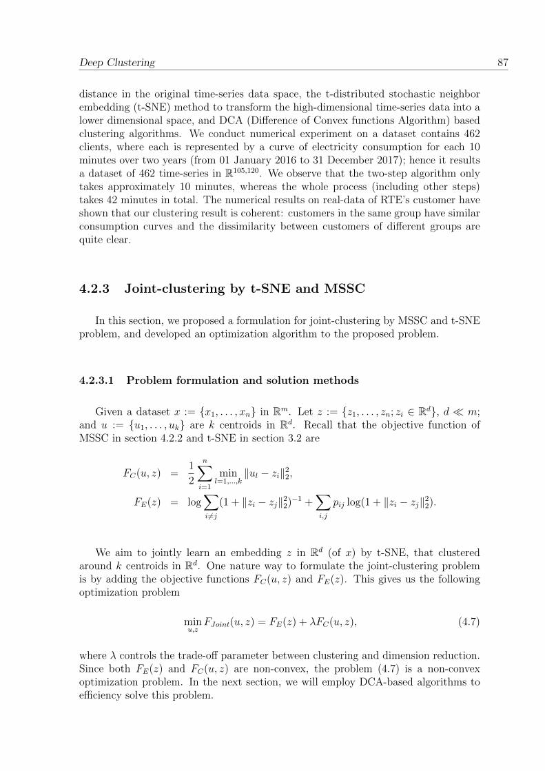
Deep Clustering 87
distance in the original time-series data space, the t-distributed stochastic neighborembedding (t-SNE) method to transform the high-dimensional time-series data into alower dimensional space, and DCA (Difference of Convex functions Algorithm) basedclustering algorithms. We conduct numerical experiment on a dataset contains 462clients, where each is represented by a curve of electricity consumption for each 10minutes over two years (from 01 January 2016 to 31 December 2017); hence it resultsa dataset of 462 time-series in R105,120. We observe that the two-step algorithm onlytakes approximately 10 minutes, whereas the whole process (including other steps)takes 42 minutes in total. The numerical results on real-data of RTE’s customer haveshown that our clustering result is coherent: customers in the same group have similarconsumption curves and the dissimilarity between customers of different groups arequite clear.
4.2.3 Joint-clustering by t-SNE and MSSC
In this section, we proposed a formulation for joint-clustering by MSSC and t-SNEproblem, and developed an optimization algorithm to the proposed problem.
4.2.3.1 Problem formulation and solution methods
Given a dataset x := x1, . . . , xn in Rm. Let z := z1, . . . , zn; zi ∈ Rd, d m;and u := u1, . . . , uk are k centroids in Rd. Recall that the objective function ofMSSC in section 4.2.2 and t-SNE in section 3.2 are
FC(u, z) =1
2
n∑i=1
minl=1,...,k
‖ul − zi‖22,
FE(z) = log∑i6=j
(1 + ‖zi − zj‖22)−1 +
∑i,j
pij log(1 + ‖zi − zj‖22).
We aim to jointly learn an embedding z in Rd (of x) by t-SNE, that clusteredaround k centroids in Rd. One nature way to formulate the joint-clustering problemis by adding the objective functions FC(u, z) and FE(z). This gives us the followingoptimization problem
minu,z
FJoint(u, z) = FE(z) + λFC(u, z), (4.7)
where λ controls the trade-off parameter between clustering and dimension reduction.Since both FE(z) and FC(u, z) are non-convex, the problem (4.7) is a non-convexoptimization problem. In the next section, we will employ DCA-based algorithms toefficiency solve this problem.
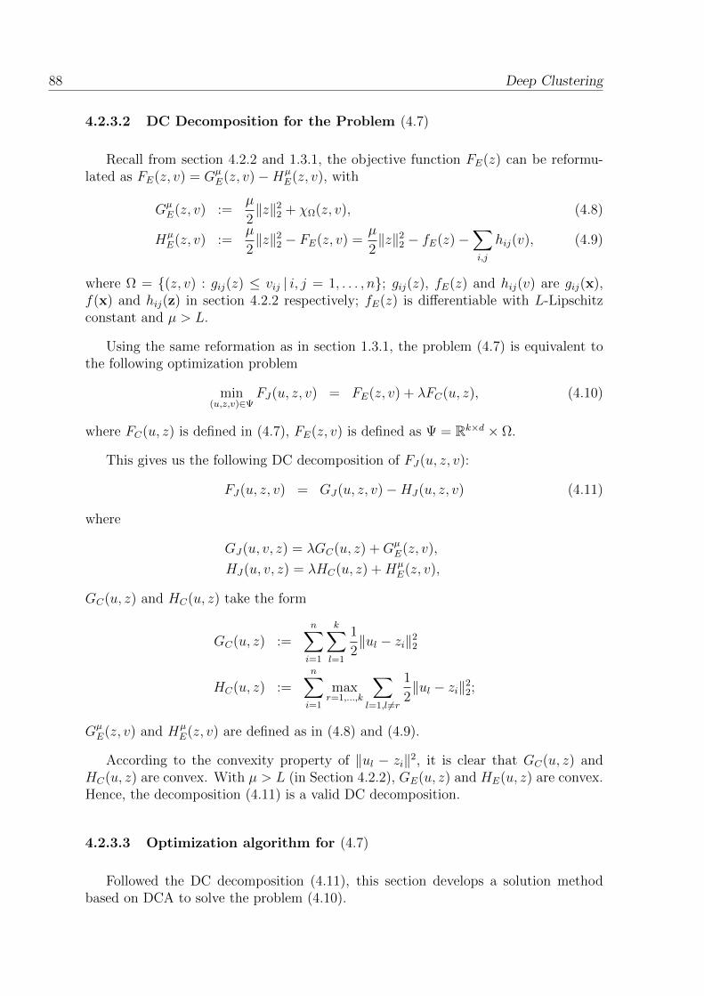
88 Deep Clustering
4.2.3.2 DC Decomposition for the Problem (4.7)
Recall from section 4.2.2 and 1.3.1, the objective function FE(z) can be reformu-lated as FE(z, v) = Gµ
E(z, v)−HµE(z, v), with
GµE(z, v) :=
µ
2‖z‖2
2 + χΩ(z, v), (4.8)
HµE(z, v) :=
µ
2‖z‖2
2 − FE(z, v) =µ
2‖z‖2
2 − fE(z)−∑i,j
hij(v), (4.9)
where Ω = (z, v) : gij(z) ≤ vij | i, j = 1, . . . , n; gij(z), fE(z) and hij(v) are gij(x),f(x) and hij(z) in section 4.2.2 respectively; fE(z) is differentiable with L-Lipschitzconstant and µ > L.
Using the same reformation as in section 1.3.1, the problem (4.7) is equivalent tothe following optimization problem
min(u,z,v)∈Ψ
FJ(u, z, v) = FE(z, v) + λFC(u, z), (4.10)
where FC(u, z) is defined in (4.7), FE(z, v) is defined as Ψ = Rk×d × Ω.
This gives us the following DC decomposition of FJ(u, z, v):
FJ(u, z, v) = GJ(u, z, v)−HJ(u, z, v) (4.11)
where
GJ(u, v, z) = λGC(u, z) +GµE(z, v),
HJ(u, v, z) = λHC(u, z) +HµE(z, v),
GC(u, z) and HC(u, z) take the form
GC(u, z) :=n∑i=1
k∑l=1
1
2‖ul − zi‖2
2
HC(u, z) :=n∑i=1
maxr=1,...,k
∑l=1,l 6=r
1
2‖ul − zi‖2
2;
GµE(z, v) and Hµ
E(z, v) are defined as in (4.8) and (4.9).
According to the convexity property of ‖ul − zi‖2, it is clear that GC(u, z) andHC(u, z) are convex. With µ > L (in Section 4.2.2), GE(u, z) and HE(u, z) are convex.Hence, the decomposition (4.11) is a valid DC decomposition.
4.2.3.3 Optimization algorithm for (4.7)
Followed the DC decomposition (4.11), this section develops a solution methodbased on DCA to solve the problem (4.10).
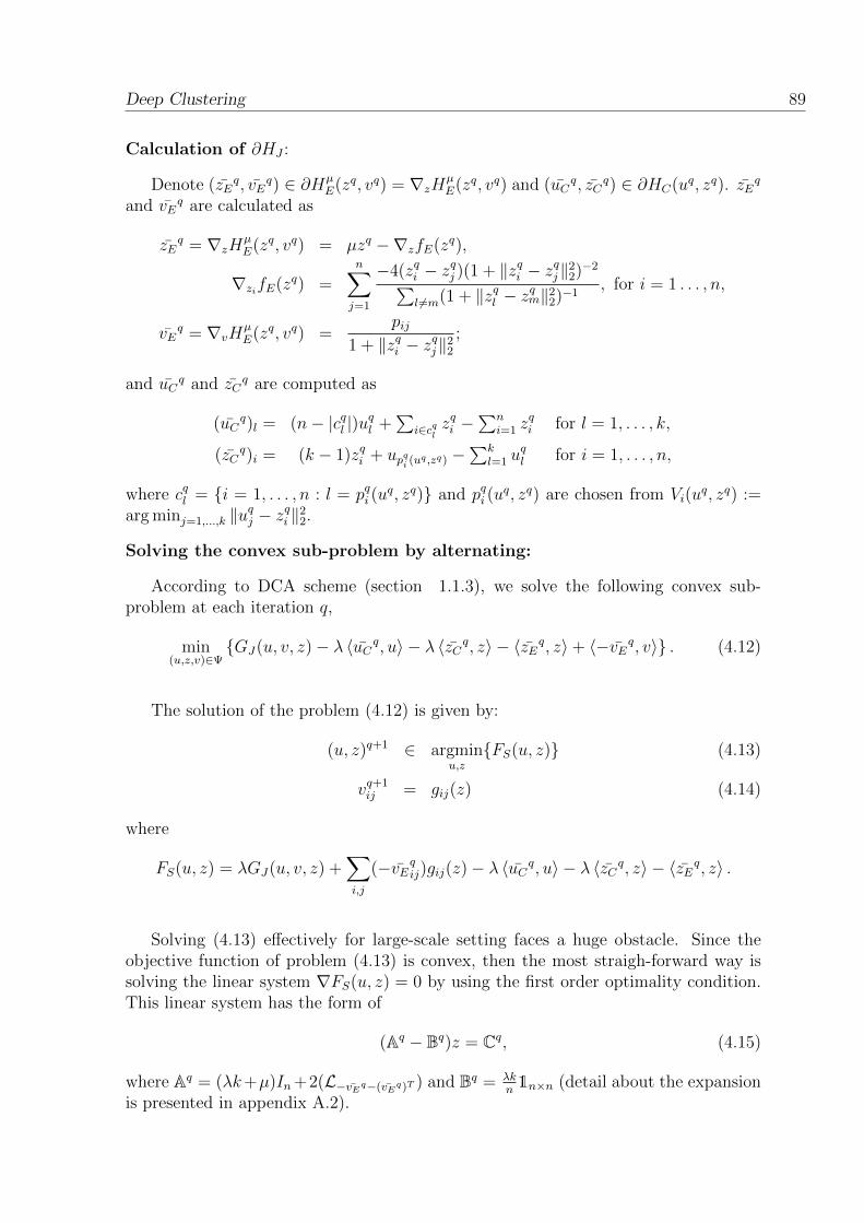
Deep Clustering 89
Calculation of ∂HJ :
Denote (zEq, vE
q) ∈ ∂HµE(zq, vq) = ∇zH
µE(zq, vq) and (uC
q, zCq) ∈ ∂HC(uq, zq). zE
q
and vEq are calculated as
zEq = ∇zH
µE(zq, vq) = µzq −∇zfE(zq),
∇zifE(zq) =n∑j=1
−4(zqi − zqj )(1 + ‖zqi − z
qj‖2
2)−2∑l 6=m(1 + ‖zql − z
qm‖2
2)−1, for i = 1 . . . , n,
vEq = ∇vH
µE(zq, vq) =
pij1 + ‖zqi − z
qj‖2
2
;
and uCq and zC
q are computed as
(uCq)l = (n− |cql |)u
ql +
∑i∈cql
zqi −∑n
i=1 zqi for l = 1, . . . , k,
(zCq)i = (k − 1)zqi + upqi (uq ,zq) −
∑kl=1 u
ql for i = 1, . . . , n,
where cql = i = 1, . . . , n : l = pqi (uq, zq) and pqi (u
q, zq) are chosen from Vi(uq, zq) :=
arg minj=1,...,k ‖uqj − z
qi ‖2
2.
Solving the convex sub-problem by alternating:
According to DCA scheme (section 1.1.3), we solve the following convex sub-problem at each iteration q,
min(u,z,v)∈Ψ
GJ(u, v, z)− λ 〈uCq, u〉 − λ 〈zCq, z〉 − 〈zEq, z〉+ 〈−vEq, v〉 . (4.12)
The solution of the problem (4.12) is given by:
(u, z)q+1 ∈ argminu,zFS(u, z) (4.13)
vq+1ij = gij(z) (4.14)
where
FS(u, z) = λGJ(u, v, z) +∑i,j
(−vEqij)gij(z)− λ 〈uCq, u〉 − λ 〈zCq, z〉 − 〈zEq, z〉 .
Solving (4.13) effectively for large-scale setting faces a huge obstacle. Since theobjective function of problem (4.13) is convex, then the most straigh-forward way issolving the linear system ∇FS(u, z) = 0 by using the first order optimality condition.This linear system has the form of
(Aq − Bq)z = Cq, (4.15)
where Aq = (λk+µ)In+2(L−vEq−(vEq)T ) and Bq = λkn1n×n (detail about the expansion
is presented in appendix A.2).
90 Deep Clustering
In practice, Aq is a sparse matrix in case the proximity matrix P is sparse, but theAq − Bq is a full matrix as Bq is a full matrix. Storing Aq − Bq is memory-intensive,as the space complexity for storing it is O(n2) regardless of the sparsity of matrix P(hence Aq). As for n = 70, 000 yields the total size of 36, 5 GB of RAM for the matrixAq − Bq, hence this algorithm can not scale for bigger dataset. One may argue thatAq−Bq could be stored in custom “sparse” matrix format where the “sparse” elementis λk/n (or 1 if we divide both sides of the linear system by λk/n) instead of 0 instandard sparse matrix, but it is complex and difficult to apply existing powerful toolsfor solving the huge system of equation (Aq − Bq)z = Cq.
Hence, in order to exploit the sparsity structure of the matrix P , we employ alter-nating optimization algorithm to solve the convex sub-problem (4.13). Each alternat-ing iteration t of problem (4.13) requires solving two convex sub-problems as
uq,t+1 ∈ argminu
GC(u, zq,t+1)− 〈uCq, u〉
, (4.16)
and
zq,t+1 ∈ argminz
λGC(uq,t, z) +
µ
2‖z‖2 − λ 〈zCq, z〉 − 〈zEq, z〉+
∑i,j
(−vEqij)gij(z)
.
(4.17)
Since the objective function of problem (4.16) is convex, then according to the firstorder optimality condition, its solution can be obtained by solving ∇uGC(u, zq,t+1) −uC
q = 0. Hence, uq,t+1 is computed as
uq,t+1 =1
n
(uC
q + 1k×nzq,t+1
). (4.18)
Solving (4.17) is equivalent to solving the following linear system
Dq,tz =(λzC
q + zEq + λ1n×ku
q,t), (4.19)
where Dq,t =((λk + µ)In + 2(L−vEq−(vEq)T )
), LA is a Rn×n matrix with (LA)ij = −Aij
if i 6= j and −Aii +∑n
l=1 Ail otherwise. For the detailed expansion to acquire (4.19),refer to section A.3. Algorithm for solving the problem (4.12) is detailed in Algorithm4.3.
Solving (4.13) has double advantages. Beside the memory issue, algorithm 4.3 ispotentially faster than solving (4.15). The best alogrithm for solving the linear system(4.15) has the complexity O(n2.376) since (Aq − Bq) is a full matrix. On the otherhand, since the sparse matrix P has at most (2kn) non-zero elements (where k is thek-nearest neighbor paramter for computing P ), hence the matrix Dq,t of (4.19) has atmost (2k + 1)n non-zero elements. Algorithm 4.3 runs for t iterations, each has thecomplexity of O((2k+ 1)
√κn)) ([98], by Conjugate Gradient method), where κ is the
condition number of Dq,t. Since we add (λk+µ) to the diagonal of Dq,t, the κ of Dq,t issmall. In addition, the number of neighbor are often small (k n, i.e k = 5). Hence,for a large value of n, this is an huge improvement in terms of running time.

Deep Clustering 91
Algorithm 4.3 Algorithm for solving the problem (4.12)
Input: uq,0, zq,0, λOutput: u∗, z∗
Initialization: t← 0.repeat
Compute zq,t+1 by solving (4.19).Compute uq,t+1 = 1
n(uC
q + 1k×nzq,t+1).
t← t+ 1.until Stopping condition.Output (z∗, u∗) = (zq,t, uq,t)
DCA-Like for problem (4.7):
The DCA for solving the problem (4.7) is described in Algorithm 4.4. However,based on the advantages of DCA-Like over DCA for t-SNE problem in chapter 3, weconsider DCA-Like for solving the problem (4.7).
Algorithm 4.4 DCA for solving problem (4.7)
Initialization: Choose u0, z0, µ > L and q ← 0.repeat
Compute (zEq, vE
q) ∈ ∂HµqE (zq, vq) and (uC
q, zCq) ∈ ∂HC(uq, zq).
Obtain (zq+1, uq+1) by using Algorithm (4.3).q ← q + 1.
until Stopping condition.
At each iteration q, DCA-Like requires µq satisfies the following condition:
HJ(uq+1, zq+1, vq+1) ≥ HJ(uq, zq, vq) + 〈uJq, uq+1 − uq〉+ 〈vJq, vq+1 − vq〉+ 〈zJq, zq+1 − zq〉 (4.20)
where (uJq, vJ
q, zJq) ∈ ∂HJ(uq, vq, zq). Hence, in compare to Algorithm 4.4, we only
need to search for µ = µq such that the inequality (4.20) holds at (zq+1, uq+1, vq+1).The condition (4.20) is detailed in (4.21). The strategy to update µq is described inAlogrithm 4.5.
In detail, condition (4.20) is expanded as
UµqE (zq, zq+1)− λUC(uq, zq, uq+1, zq+1) ≥ FE(xq+1)− λHC(zq+1, uq+1), (4.21)
where
UµqE (zq, zq+1) = FE(zq) +
⟨∇fE(zq), zq+1 − zq
⟩+µq2‖zq+1 − zq‖2 −
⟨vE
q, g(zq+1)− g(zq)⟩,
UC(uq, zq, uq+1, zq+1) = HC(uq, zq) +⟨∇HC(zq, uq), (zq+1 − zq, uq+1 − uq)
⟩.
Proposition 4.1. Let g(z) = gi,j(z)i,j=1,...,n, φ = (u, z, g(z)). The sequence φqgenerated by Algorithm 4.5 enjoys the following properties:
92 Deep Clustering
Algorithm 4.5 MSSC-JDR: DCA-Like for solving problem (4.7)
Initialization: Choose u0, z0, η > 1, 0 < δ < 1, µ0 > 0 and q ← 0.repeat
Compute (zEq, vE
q) ∈ ∂HµqE (zq, vq) and (uC
q, zCq) ∈ ∂HC(uq, zq).
Set µq = maxµ0, δµq−1.Obtain (zq+1, uq+1) by using Algorithm (4.3).while U
µqE (zq, zq+1)− λUC(uq, zq, uq+1, zq+1) < FE(xq+1)− λHC(zq+1, uq+1) do
µq ← ηµqObtain (zq+1, uq+1) by using Algorithm (4.3).
end whileq ← q + 1.
until Stopping condition.
(i) The sequence FJ(φq) is decreasing;
(ii) If FJ(φq+1) = FJ(φq), then φq is a critical point of (4.10) and Algorithm 4.5terminates at the q-th iteration.
(iii) If µ(G) + µ(H) > 0 then the series ‖φq+1 − φq‖2 converges.
Proof. Direct consequences of the convergence properties of DCA-Like in [51] and[80].
4.2.4 Numerical experiment
4.2.4.1 Experiment settings and Datasets
Evaluation criteria:
Given an input xi with ground-truth label li; and pi is the assignment label fromclustering algorithm, we measure the following criteria to evaluate experimental results:
— Clustering Accuracy (ACC [13]): ACC is calculated as ACC(l, p) =1n
∑ni=1 1m(pi)=li , where m(xi) is the function which maps each clustering as-
sign in pi to the equivalent label li. In our case, we use the mapping by usingthe Kuhn-Munkres algorithm [73].
— Normalized mutual information (NMI [102]): The NMI criterion is cal-
culated as NMI(l, p) = I(l,p)√H(l)H(p)
, where I(l, p) is the mutual information of l
and p.
In addition, we measure running time (in seconds) to evaluate the speed of algo-rithms. All experiments are conducted on a Intel(R) Xeon (R) CPU E5-2630 v4 @2.20GHz with 32GB of RAM and a GTX 1080 GPU.
We repeat the experiment 10 times, and report the average with standard deviationof each criterion.
D
Deep Clustering 93
Setting for MSSC-2S and MSSC-JDR: following the work of [51, 123], we set µ0 =10−6. For all datasets, proximity matrix P is constructed by k-Nearest Neighbor withkNN = 10. z0 is draw from N (0, 10−8). Early exaggeration technique [106] is deployedfor first 20 iterations with the constant value of 4. For MSSC-2S, we execute t-SNE untilconvergence, then clustering on z by MSSC 10 times, choosing the solution which hasthe best objective value. For MSSC-JDR, we initialize zMSSC-JDR0 from the 5th iteration oft-SNE after early exaggeration. uMSSC-JDR0 is obtained by executing MSSC 10 times onzMSSC-JDR0 and choose the solution with the lowest objective value. The linear system ofthe sub-problem is solved by Conjugate Gradient solver with the complexity of O(n).
Datasets: Datasets used in the experiment are downloaded from Feature SelectionRepository 2 and UCI Repository 3.
4.2.4.2 Experiment 1: Hyper-parameters of MSSC-JDR and MSSC-2S
In this experiment, we interest in the performance of MSSC-JDR and MSSC-2S astheir hyper-parameters vary: λ for MSSC-JDR and d for both algorithms.
For this experiment, we vary λ ∈ 10−4, 10−3, . . . , 1 and d ∈ 5, 10, 20, 30. Clus-tering accuracy is reported in Figure 4.1 for 6 datasets (leukemia, GLI 85, Carcinom,coil20, isolet and gisette), due to the large grid-search used in this experiment.
We observe that:
- For MSSC-2S, the number of dimensions has a strong effect on the clusteringaccuracy. In detail, for d ∈ 20, 30, MSSC-2S produces the highest clustering accuracyin 4 over 6 cases (leukemia, coil20, gissete and usps); which is higher than d ∈ 5, 10by 1 case.
- For MSSC-JDR, both λ and d strongly affect clustering accuracy. In detail, thehighest accuracy is mostly obtained for d = 20 in 4 over 6 cases (leukemia, coil20,isolet, and usps); followed by d = 10 for 3 over 4 cases (leukemia, coil20 and usps).For d = 20, λ = 10−2 produces the best result with the highest accuracy in 4 over6 cases (leukemia, Carcinom, coil20, isolet, gissete, and usps); followed by λ = 10−1
with 3 over 4 cases (leukemia, Carcinom, and gissete).
From these observations, we choose d = 10 (for both MSSC-JDR and MSSC-2S) andλ = 10−2 (for MSSC-JDR) in the next experiments.
4.2.4.3 Experiment 2: Comparasion between MSSC-2S, MSSC-JDR and stan-dard MSSC
In this experiment, we interest in studying the effectiveness of MSSC-2S andMSSC-JDR in compare with the standard MSSC algorithm [45], to demonstrate the ef-
2. http://featureselection.asu.edu/index.php
3. https://archive.ics.uci.edu/ml/datasets/isolet

94D
eep
Clu
ster
ing
MSSC-2S
MSSC-JDR=10-4
MSSC-JDR=10-3
MSSC-JDR=10-2
MSSC-JDR=10-1
MSSC-JDR=100
7374757677787980Accuracy (%)
d =
5d
= 1
0d
= 2
0d
= 3
0
(a)
leu
kem
ia
MSSC-2S
MSSC-JDR=10-4
MSSC-JDR=10-3
MSSC-JDR=10-2
MSSC-JDR=10-1
MSSC-JDR=100
80
80.581
81.582
82.5
Accuracy (%)(b
)C
arc
inom
MSSC-2S
MSSC-JDR=10-4
MSSC-JDR=10-3
MSSC-JDR=10-2
MSSC-JDR=10-1
MSSC-JDR=100
6870727476788082
Accuracy (%)
(c)
coil
20
MSSC-2S
MSSC-JDR=10-4
MSSC-JDR=10-3
MSSC-JDR=10-2
MSSC-JDR=10-1
MSSC-JDR=100
58606264666870Accuracy (%)
(d)
isole
t
MSSC-2S
MSSC-JDR=10-4
MSSC-JDR=10-3
MSSC-JDR=10-2
MSSC-JDR=10-1
MSSC-JDR=100
93.2
93.3
93.4
93.5
93.6
93.7
Accuracy (%)
(e)
giss
ete
MSSC-2S
MSSC-JDR=10-4
MSSC-JDR=10-3
MSSC-JDR=10-2
MSSC-JDR=10-1
MSSC-JDR=100
95.8
95.996
96.1
96.2
96.3
96.4
Accuracy (%)
(f)
usp
s
Fig
ure
4.1
–C
lust
erin
gac
cura
cyof
MSSC-2S
andMSSC-JDR
asλ
vari
es.
\' \' \'
\' \' \'
\' \' \'
\' \'
\'
\' \' \'
\' \' \'
\' \' \'
\' \' \'
w \' \'
\'
\' 1 ~ 1 \' / / / 1 1 \'

Deep Clustering 95
fectiveness of our proposed method.
Parameters of MSSC-2S and MSSC-JDR are the same as in the Experiment 1, butwith the number of reduced dimension d = 10 for both algorithms and λ = 10−2 forMSSC-JDR.
The comparative results between algorithms are reported in Table 4.1 and Fig-ure 4.2.
In comparison between MSSC-2S and MSSC-JDR:— In terms of clustering accuracy, both MSSC-2S and MSSC-JDR are clearly better
than MSSC in all datasets. The gain is high, from 6.95% (isolet) to 48.42%(emnist-digits).
— In terms of running time, in general, both MSSC-2S and MSSC-JDR are slowerthan MSSC. However, MSSC-JDR is faster than MSSC for 2 biggest datasets (mnistand emnist-digits). It is worthy to note that the running time for small-sizedatasets is quite small (lower than 15 minutes), but the save-up in terms ofrunning time for large-scale datasets is enormous: from 8.8 hours (reps. 80minutes) to 1.5 hours (reps. 10.5 minutes) for emnist-digits dataset (reps. mnistdataset).
In comparison between MSSC-JDR and MSSC-2S, MSSC-JDR proved to be more effi-cient, in both terms of clustering quality and running time. In terms of the clusteringaccuracy, MSSC-JDR is better than MSSC-2S in 7 over 9 datasets (from 0.01% to 1.09%),and equal in the remaining 2 datasets (leukemia and GLI 85 ). As for running time,except for 2 datasets (isolet and gisette), MSSC-JDR is faster than MSSC-2S by a largemargin, up to 14 times. Most notably, in the three largest datasets (usps, mnist andemnist-digits), the gains are from 3.17 to 14 times, with no drop in accuracy.
In short, both MSSC-2S and MSSC-JDR out-perform MSSC in term of accuracy (upto 48.42%) but with a trade-off in term of computing time. This result is aligned withprevious result on clustering high-dimensional data: the dimension reduction techniqueimproves the clustering accuracy by reducing the number of dimension to cope with“curse of dimensionality” phenomenal. MSSC-JDR is clearly an enhancement of MSSCfor high-dimensional datasets with an agreeable trade-off in terms of computing time;and MSSC-JDR also clearly is an improvement over MSSC-2S.
4.2.4.4 Experiment 3: Comparison with NMF and VolMin-based factor-ization joint-clustering algorithms
Comparative algorithms and settings: This experiment compares the per-formance between our proposed method with jointly dimension reduction and MSSC-based clustering algorithms. We consider the following algorithms:
— NMFKM [119]: Two-stage combination of NMF and K-means.— JNKM [119]: Joint NMF and K-means.— JVKM [119]: Joint VolMin and K-means.For JNKM and JVKM, the parameters for this experiments is the number of reduced

96 Deep Clustering
dimensions F . We choose F ∈ 5, 10, 20, 30 and report the best average result. Othersparameters are set as default provided by the authors’ source code.
Parameters of MSSC-JDR are the same as in Experiment 1, but with the number ofreduced dimension d = 10 and λ = 10−2.
Experiment result and comments: The comparative results between algo-rithms are reported in Table 4.1 and Figure 4.2. We observe that MSSC-JDR out-performs others by a large margin in term of clustering accuracy but requires longerrunning time. The gains in clustering accuracy depends on the datasets, but MSSC-JDRis always better or equal: from no gains at all (as in GLI 85 dataset) up to 38% (asin mnist dataset). In terms of computing time, the same situation as in comparisonwith MSSC: the improvement in term of clustering accuracy comes with a trade-off butreasonable computing time.
To sum up, MSSC-JDR is the most accurate clustering algorithm among MSSC-JDR,MSSC-2S and MSSC.
leukemia GLI_85 Carcinom coil20 isolet gisette usps mnist emnist-digits10
20
30
40
50
60
70
80
90
100
Acc
urac
y (%
)
MSSCJNKMJVKMNMFKMMSSC-2SMSSC-JDR
Figure 4.2 – Clustering accuracy of all algorithms. For the last dataset (emnist-digits), JNKM and JVKM encounter the Out Of Memory error.
Table 4.1 – Comparative result between algorithms over all datasets. Bold valuescorrespond to best results for each dataset. NA means the algorithm failed to procedurethe result (i.e. Out of Memory).
Dataset AlgorithmNMI Accuracy Time (sec.)
Average STD Average STD Average STD
leukemia MSSC 12.54% 0.00% 70.83% 0.00% 1.44 0.05
- ·-I-·· - ·-I-·· - ·-I-·· - ·-I-·· -+--+-
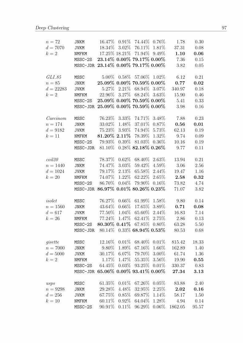
Deep Clustering 97
n = 72 JNKM 16.47% 0.91% 74.44% 0.76% 1.78 0.30d = 7070 JVKM 18.34% 3.02% 76.11% 1.81% 37.31 0.08k = 2 NMFKM 17.25% 18.21% 71.94% 9.49% 1.10 0.06
MSSC-2S 23.14% 0.00% 79.17% 0.00% 7.36 0.15MSSC-JDR 23.14% 0.00% 79.17% 0.00% 3.82 0.05
GLI 85 MSSC 5.00% 0.58% 57.06% 1.02% 6.12 0.21n = 85 JNKM 25.09% 0.00% 70.59% 0.00% 0.77 0.02d = 22283 JVKM 5.27% 2.21% 68.94% 3.07% 340.97 0.18k = 2 NMFKM 22.96% 3.27% 68.24% 3.63% 15.90 0.46
MSSC-2S 25.09% 0.00% 70.59% 0.00% 5.41 0.33MSSC-JDR 25.09% 0.00% 70.59% 0.00% 3.98 0.16
Carcinom MSSC 76.23% 3.33% 74.71% 3.48% 7.88 0.23n = 174 JNKM 33.02% 1.48% 37.01% 0.87% 0.56 0.01d = 9182 JVKM 75.23% 3.93% 74.94% 5.73% 62.13 0.19k = 11 NMFKM 81.20% 2.11% 78.39% 1.32% 9.74 0.09
MSSC-2S 79.93% 0.39% 81.03% 0.36% 10.16 0.19MSSC-JDR 81.10% 0.28% 82.18% 0.26% 9.77 0.11
coil20 MSSC 78.37% 0.62% 68.40% 2.63% 13.94 0.21n = 1440 JNKM 74.47% 3.03% 59.42% 4.59% 3.06 2.56d = 1024 JVKM 79.17% 2.13% 65.58% 2.44% 19.47 1.16k = 20 NMFKM 74.07% 1.22% 62.22% 2.65% 2.58 0.32
MSSC-2S 86.70% 0.04% 79.90% 0.16% 73.82 4.74MSSC-JDR 86.97% 0.01% 80.26% 0.23% 71.07 3.82
isolet MSSC 76.27% 0.66% 61.99% 1.58% 9.80 0.14n = 1560 JNKM 43.64% 0.66% 17.65% 3.89% 0.71 0.08d = 617 JVKM 77.50% 1.04% 65.60% 2.44% 16.83 7.14k = 26 NMFKM 77.24% 1.47% 62.41% 2.75% 2.86 0.13
MSSC-2S 80.30% 0.41% 67.85% 0.80% 63.28 5.50MSSC-JDR 80.14% 0.33% 68.94% 0.53% 80.53 0.68
gisette MSSC 12.16% 0.01% 68.40% 0.01% 815.42 18.33n = 7000 JNKM 9.80% 1.89% 67.16% 1.66% 162.89 1.40d = 5000 JVKM 30.17% 6.07% 79.70% 3.00% 61.74 1.36k = 2 NMFKM 1.17% 1.47% 55.35% 3.56% 19.90 0.55
MSSC-2S 64.45% 0.03% 93.25% 0.01% 330.37 0.83MSSC-JDR 65.06% 0.00% 93.41% 0.00% 27.34 3.13
usps MSSC 61.35% 0.01% 67.26% 0.05% 83.88 2.40n = 9298 JNKM 29.28% 4.48% 32.95% 2.25% 2.02 0.16d = 256 JVKM 67.75% 0.85% 69.87% 1.14% 58.17 1.50k = 10 NMFKM 60.11% 0.92% 64.04% 1.28% 4.94 0.14
MSSC-2S 90.91% 0.11% 96.29% 0.06% 1862.05 95.57

98 Deep Clustering
MSSC-JDR 90.92% 0.13% 96.30% 0.07% 583.97 41.56
mnist MSSC 44.25% 0.02% 48.24% 0.05% 4774.27 171.50n = 70000 JNKM 23.73% 2.26% 30.33% 2.60% 31.96 10.55d = 784 JVKM 49.94% 1.00% 58.65% 2.26% 201.61 3.50k = 10 NMFKM 44.36% 2.21% 50.89% 4.10% 95.36 3.25
MSSC-2S 91.41% 0.01% 96.63% 0.00% 2294.60 49.17MSSC-JDR 91.46% 0.03% 96.66% 0.01% 630.52 24.49
emnist-digits MSSC 42.86% 0.01% 46.78% 0.00% 31816.56 1,013.58n = 280000 JNKM NA NA NA NA NA NAd = 784 JVKM NA NA NA NA NA NAk = 10 NMFKM 36.67% 0.45% 26.23% 0.63% 274.79 3.61
MSSC-2S 94.35% 0.01% 97.97% 0.01% 78962.85 5078.14MSSC-JDR 94.36% 0.00% 97.97% 0.00% 5623.78 691.53
4.2.4.5 Experiment 4: Compare with joint-clustering algorithms usingauto-encoder
This experiment compares our proposed approach with auto-encoder-based joint-clustering algorithms on image datasets. We consider the following ones:
— DC-Kmeans [104] proposes an algorithm for solving the joint-clustering of DeepAuto-Encoder and K-means by Alternating Direction of Multiplier Method(ADMM).
— DEC [117] uses a two-step procedure: the first step consists of training the auto-encoder using reconstruction loss; then the second step jointly optimizes theencoder and soft assignment clustering loss function for dimension reductionand clustering respectively.
— IDEC [33] (Improved DEC) argues the two-step procedure in DEC could weakenthe representatives of the embedded features and hurts clustering performancesas DEC strips out the decoder part during the optimization the joint-clustering;hence it simultaneously optimizes the full auto-encoder and clustering by softassignment clustering as in DEC.
Setting for DC-Kmeans: we use the authors’ implementation 4. We set the numberof neural in the bottle-neck layer equals to the number of classes for all datasets. Fortraining the auto-encoder, we use Matlab’s neural network toolbox. We also noticethat the author’s scheme for initializing K-means’ centroids often produces bad results(especially for coil20 dataset), so we use to the same procedure for initial point asMSSC-JDR.
4. https://github.com/JennyQQL/DeepClusterADMM-Release
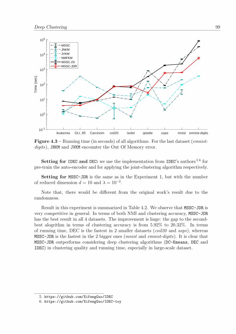
Deep Clustering 99
leukemia GLI_85 Carcinom coil20 isolet gisette usps mnist emnist-digits10-1
100
101
102
103
104
105T
ime
(sec
)
MSSCJNKMJVKMNMFKMMSSC-2SMSSC-JDR
Figure 4.3 – Running time (in seconds) of all algorithms. For the last dataset (emnist-digits), JNKM and JVKM encounter the Out Of Memory error.
Setting for IDEC and DEC: we use the implementation from IDEC’s authors 5 6 forpre-train the auto-encoder and for applying the joint-clustering algorithm respectively.
Setting for MSSC-JDR is the same as in the Experiment 1, but with the numberof reduced dimension d = 10 and λ = 10−2.
Note that, there would be different from the original work’s result due to therandomness.
Result in this experiment is summarized in Table 4.2. We observe that MSSC-JDR isvery competitive in general. In terms of both NMI and clustering accuracy, MSSC-JDRhas the best result in all 4 datasets. The improvement is huge: the gap to the second-best alogrithm in terms of clustering accuracy is from 5.92% to 20.32%. In termsof running time, DEC is the fastest in 2 smaller datasets (coil20 and usps), whereasMSSC-JDR is the fastest in the 2 bigger ones (mnist and emnist-digits). It is clear thatMSSC-JDR outperforms considering deep clustering algorithms (DC-Kmeans, DEC andIDEC) in clustering quality and running time, especially in large-scale dataset.
5. https://github.com/XifengGuo/IDEC
6. https://github.com/XifengGuo/IDEC-toy
/ / ____ .,,..
' . ,,,,,.,.. ·' . . ·-wf ,,.--· ..,,,.--• I .t-·-· • ·-·-· -·""· /
/,-...__ .... . ,.,_ i ·--· / \ / ,. ----- ________ _-_:-_-- j;· ; _,., \ / ,I b,.</ . . .......... :-t~ -~ _.,// ·--~-,.,<,/ 2 ...... .-- .... . . . ..... . __ --·-- ·,. / ~/ . _____ ,,,. '·..f
.r, I' • . ' / .
/ '· . ' I' • .L. ..... ....
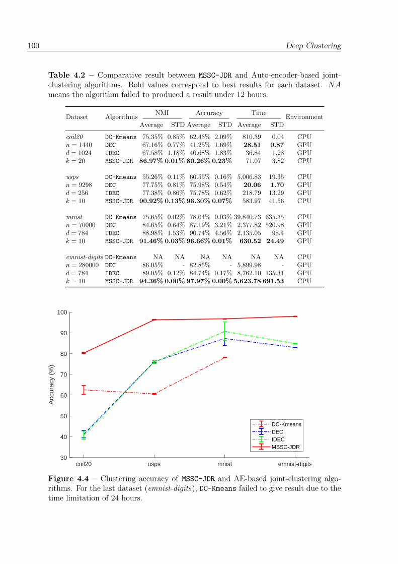
100 Deep Clustering
Table 4.2 – Comparative result between MSSC-JDR and Auto-encoder-based joint-clustering algorithms. Bold values correspond to best results for each dataset. NAmeans the algorithm failed to produced a result under 12 hours.
Dataset AlgorithmsNMI Accuracy Time
EnvironmentAverage STD Average STD Average STD
coil20 DC-Kmeans 75.35% 0.85% 62.43% 2.09% 810.39 0.04 CPUn = 1440 DEC 67.16% 0.77% 41.25% 1.69% 28.51 0.87 GPUd = 1024 IDEC 67.58% 1.18% 40.68% 1.83% 36.84 1.28 GPUk = 20 MSSC-JDR 86.97% 0.01% 80.26% 0.23% 71.07 3.82 CPU
usps DC-Kmeans 55.26% 0.11% 60.55% 0.16% 5,006.83 19.35 CPUn = 9298 DEC 77.75% 0.81% 75.98% 0.54% 20.06 1.70 GPUd = 256 IDEC 77.38% 0.86% 75.78% 0.62% 218.79 13.29 GPUk = 10 MSSC-JDR 90.92% 0.13% 96.30% 0.07% 583.97 41.56 CPU
mnist DC-Kmeans 75.65% 0.02% 78.04% 0.03% 39,840.73 635.35 CPUn = 70000 DEC 84.65% 0.64% 87.19% 3.21% 2,377.82 520.98 GPUd = 784 IDEC 88.98% 1.53% 90.74% 4.56% 2,135.05 98.4 GPUk = 10 MSSC-JDR 91.46% 0.03% 96.66% 0.01% 630.52 24.49 GPU
emnist-digits DC-Kmeans NA NA NA NA NA NA CPUn = 280000 DEC 86.05% - 82.85% - 5,899.98 - GPUd = 784 IDEC 89.05% 0.12% 84.74% 0.17% 8,762.10 135.31 GPUk = 10 MSSC-JDR 94.36% 0.00% 97.97% 0.00% 5,623.78 691.53 CPU
coil20 usps mnist emnist-digits30
40
50
60
70
80
90
100
Acc
urac
y (%
)
DC-KmeansDECIDECMSSC-JDR
Figure 4.4 – Clustering accuracy of MSSC-JDR and AE-based joint-clustering algo-rithms. For the last dataset (emnist-digits), DC-Kmeans failed to give result due to thetime limitation of 24 hours.
-·-:3:-·· -·-:3:-·· -·-:3:-·· -+-
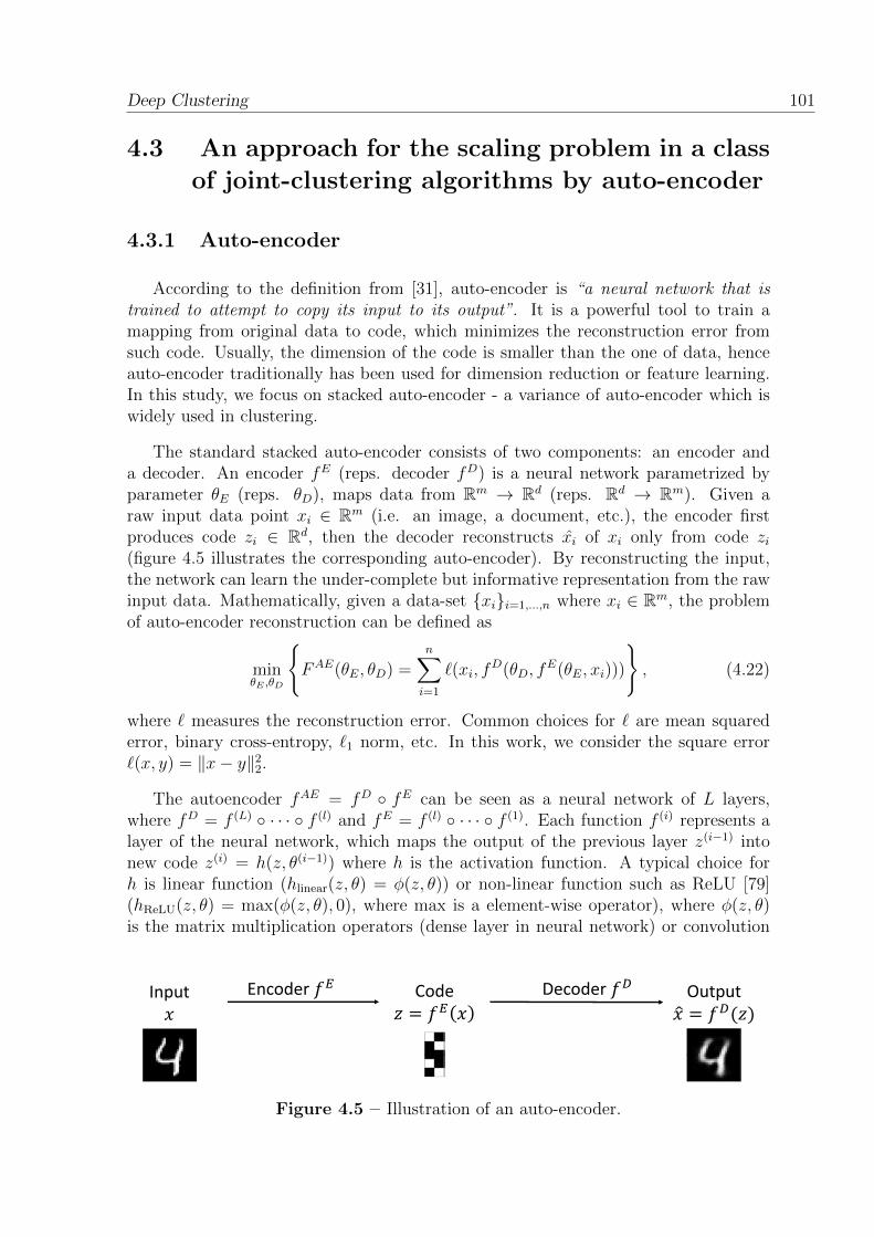
Deep Clustering 101
4.3 An approach for the scaling problem in a class
of joint-clustering algorithms by auto-encoder
4.3.1 Auto-encoder
According to the definition from [31], auto-encoder is “a neural network that istrained to attempt to copy its input to its output”. It is a powerful tool to train amapping from original data to code, which minimizes the reconstruction error fromsuch code. Usually, the dimension of the code is smaller than the one of data, henceauto-encoder traditionally has been used for dimension reduction or feature learning.In this study, we focus on stacked auto-encoder - a variance of auto-encoder which iswidely used in clustering.
The standard stacked auto-encoder consists of two components: an encoder anda decoder. An encoder fE (reps. decoder fD) is a neural network parametrized byparameter θE (reps. θD), maps data from Rm → Rd (reps. Rd → Rm). Given araw input data point xi ∈ Rm (i.e. an image, a document, etc.), the encoder firstproduces code zi ∈ Rd, then the decoder reconstructs xi of xi only from code zi(figure 4.5 illustrates the corresponding auto-encoder). By reconstructing the input,the network can learn the under-complete but informative representation from the rawinput data. Mathematically, given a data-set xii=1,...,n where xi ∈ Rm, the problemof auto-encoder reconstruction can be defined as
minθE ,θD
FAE(θE, θD) =
n∑i=1
`(xi, fD(θD, f
E(θE, xi)))
, (4.22)
where ` measures the reconstruction error. Common choices for ` are mean squarederror, binary cross-entropy, `1 norm, etc. In this work, we consider the square error`(x, y) = ‖x− y‖2
2.
The autoencoder fAE = fD fE can be seen as a neural network of L layers,where fD = f (L) · · · f (l) and fE = f (l) · · · f (1). Each function f (i) represents alayer of the neural network, which maps the output of the previous layer z(i−1) intonew code z(i) = h(z, θ(i−1)) where h is the activation function. A typical choice forh is linear function (hlinear(z, θ) = φ(z, θ)) or non-linear function such as ReLU [79](hReLU(z, θ) = max(φ(z, θ), 0), where max is a element-wise operator), where φ(z, θ)is the matrix multiplication operators (dense layer in neural network) or convolution
Code 𝑧 = 𝑓𝐸 𝑥
Input 𝑥
Output ො𝑥 = 𝑓𝐷(𝑧)
Encoder 𝑓𝐸 Decoder 𝑓𝐷
Figure 4.5 – Illustration of an auto-encoder.
( )
IJ ~
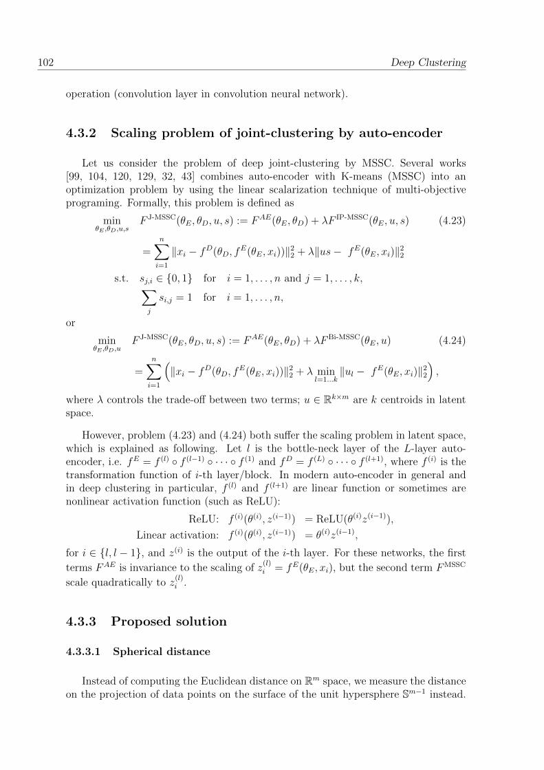
102 Deep Clustering
operation (convolution layer in convolution neural network).
4.3.2 Scaling problem of joint-clustering by auto-encoder
Let us consider the problem of deep joint-clustering by MSSC. Several works[99, 104, 120, 129, 32, 43] combines auto-encoder with K-means (MSSC) into anoptimization problem by using the linear scalarization technique of multi-objectiveprograming. Formally, this problem is defined as
minθE ,θD,u,s
F J-MSSC(θE, θD, u, s) := FAE(θE, θD) + λF IP-MSSC(θE, u, s) (4.23)
=n∑i=1
‖xi − fD(θD, fE(θE, xi))‖2
2 + λ‖us− fE(θE, xi)‖22
s.t. sj,i ∈ 0, 1 for i = 1, . . . , n and j = 1, . . . , k,∑j
si,j = 1 for i = 1, . . . , n,
or
minθE ,θD,u
F J-MSSC(θE, θD, u, s) := FAE(θE, θD) + λFBi-MSSC(θE, u) (4.24)
=n∑i=1
(‖xi − fD(θD, f
E(θE, xi))‖22 + λ min
l=1...k‖ul − fE(θE, xi)‖2
2
),
where λ controls the trade-off between two terms; u ∈ Rk×m are k centroids in latentspace.
However, problem (4.23) and (4.24) both suffer the scaling problem in latent space,which is explained as following. Let l is the bottle-neck layer of the L-layer auto-encoder, i.e. fE = f (l) f (l−1) · · · f (1) and fD = f (L) · · · f (l+1), where f (i) is thetransformation function of i-th layer/block. In modern auto-encoder in general andin deep clustering in particular, f (l) and f (l+1) are linear function or sometimes arenonlinear activation function (such as ReLU):
ReLU: f (i)(θ(i), z(i−1)) = ReLU(θ(i)z(i−1)),
Linear activation: f (i)(θ(i), z(i−1)) = θ(i)z(i−1),
for i ∈ l, l − 1, and z(i) is the output of the i-th layer. For these networks, the first
terms FAE is invariance to the scaling of z(l)i = fE(θE, xi), but the second term FMSSC
scale quadratically to z(l)i .
4.3.3 Proposed solution
4.3.3.1 Spherical distance
Instead of computing the Euclidean distance on Rm space, we measure the distanceon the projection of data points on the surface of the unit hypersphere Sm−1 instead.
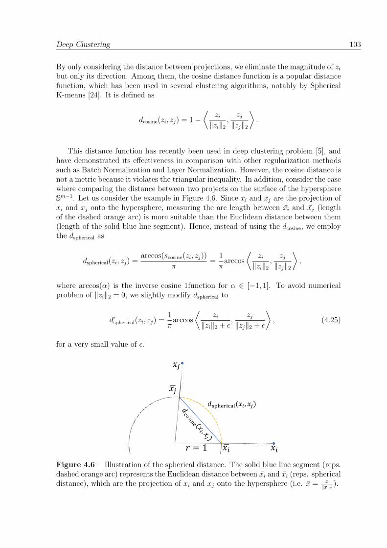
Deep Clustering 103
By only considering the distance between projections, we eliminate the magnitude of zibut only its direction. Among them, the cosine distance function is a popular distancefunction, which has been used in several clustering algorithms, notably by SphericalK-means [24]. It is defined as
dcosine(zi, zj) = 1−⟨
zi‖zi‖2
,zj‖zj‖2
⟩.
This distance function has recently been used in deep clustering problem [5], andhave demonstrated its effectiveness in comparison with other regularization methodssuch as Batch Normalization and Layer Normalization. However, the cosine distance isnot a metric because it violates the triangular inequality. In addition, consider the casewhere comparing the distance between two projects on the surface of the hypersphereSm−1. Let us consider the example in Figure 4.6. Since xi and xj are the projection ofxi and xj onto the hypersphere, measuring the arc length between xi and xj (lengthof the dashed orange arc) is more suitable than the Euclidean distance between them(length of the solid blue line segment). Hence, instead of using the dcosine, we employthe dspherical as
dspherical(zi, zj) =arccos(scosine(zi, zj))
π=
1
πarccos
⟨zi‖zi‖2
,zj‖zj‖2
⟩,
where arccos(α) is the inverse cosine 1function for α ∈ [−1, 1]. To avoid numericalproblem of ‖zi‖2 = 0, we slightly modify dspherical to
dεspherical(zi, zj) =1
πarccos
⟨zi
‖zi‖2 + ε,
zj‖zj‖2 + ε
⟩, (4.25)
for a very small value of ε.
𝑥𝑖
𝑥𝑗
ഥ𝑥𝑗
ഥ𝑥𝑖𝑟 = 1
𝑑spherical(𝑥𝑖 , 𝑥𝑗)
Figure 4.6 – Illustration of the spherical distance. The solid blue line segment (reps.dashed orange arc) represents the Euclidean distance between xi and xi (reps. sphericaldistance), which are the projection of xi and xj onto the hypersphere (i.e. x = x
‖x‖2 ).
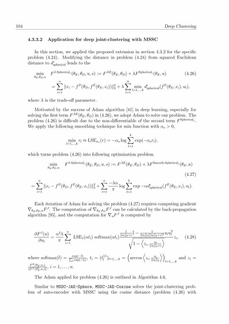
104 Deep Clustering
4.3.3.2 Application for deep joint-clustering with MSSC
In this section, we applied the proposed extension in section 4.3.2 for the specificproblem (4.24). Modifying the distance in problem (4.24) from squared Euclideandistance to dεspherical leads to the
minθE ,θD,u
F J-Sphericalε(θE, θD, u, s) := FAE(θE, θD) + λF Sphericalε(θE, u) (4.26)
=n∑i=1
‖xi − fD(θD, fE(θE, xi))‖2
2 + λ
n∑i=1
minl=1,...,k
dεspherical(fE(θE, xi), ul),
where λ is the trade-off parameter.
Motivated by the success of Adam algorithm [41] in deep learning, especially forsolving the first term FAE(θE, θD) in (4.26), we adopt Adam to solve our problem. Theproblem (4.26) is difficult due to the non-differentiable of the second term F Sphericalε .We apply the following smoothing technique for min function with αs > 0,
minl=1,...,k
rl ≈ LSEαs(r) = −αs logk∑l=1
exp(−αsrl),
which turns problem (4.26) into following optimization problem
minθE ,θD,u
F J-Sphericalε(θE, θD, u, s) := FAE(θE, θD) + λF Smooth-Sphericalε(θE, u)
(4.27)
=n∑i=1
‖xi − fD(θD, fE(θE, xi))‖2
2 +n∑i=1
−λαπ
logk∑l=1
exp−αdεspherical(fE(θE, xi), ul).
Each iteration of Adam for solving the problem (4.27) requires computing gradient∇θE ,θD,uF
J . The computation of ∇θE ,θDFJ can be calculated by the back-propagation
algorithm [95], and the computation for ∇uFJ is computed by
∂F J(u)
∂ul=α2λ
π
n∑i=1
LSE1(αti) softmax(αti)
1‖ul‖2+ε
I− 1‖ul‖2(‖ul‖2+ε)2
uluTl√
1−⟨zi,
ul‖ul‖2+ε
⟩ zi, (4.28)
where softmax(t) = exp(−t)∑l exp(−tl)
, ti = (t(i)l )l=1,...,k =
(arccos
⟨zi,
ul‖ul‖2
⟩)l=1,...,k
and zi =
FE(θE ,xi)
‖FE(θ0E ,xi)‖, i = 1, . . . , n.
The Adam applied for problem (4.26) is outlined in Algorithm 4.6.
Similar to MSSC-JAE-Sphere, MSSC-JAE-Cosine solves the joint-clustering prob-lem of auto-encoder with MSSC using the cosine distance (problem (4.26) with
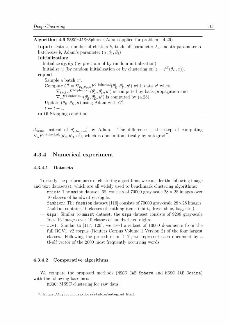
Deep Clustering 105
Algorithm 4.6 MSSC-JAE-Sphere: Adam applied for problem (4.26)
Input: Data x, number of clusters k, trade-off parameter λ, smooth parameter α,batch-size b, Adam’s parameter (α, β1, β2)Initialization:
Initialize θE, θD (by pre-train of by random initialization).Initialize u (by random initialization or by clustering on z = fE(θE, x)).
repeatSample a batch xt.Compute Gt = ∇θE ,θD,uF
J-Spherical(θtE, θtD, u
t) with data xt where∇θE ,θDF
J-Sphericalε(θtE, θtD, u
t) is computed by back-propagation and∇uF
J-Sphericalε(θtE, θtD, u
t) is computed by (4.28).Update (θE, θD, µ) using Adam with Gt.t← t+ 1.
until Stopping condition.
dcosine instead of dεspherical) by Adam. The difference is the step of computing
∇uFJ-Sphericalε(θtE, θ
tD, u
t), which is done automatically by autograd 7.
4.3.4 Numerical experiment
4.3.4.1 Datasets
To study the performances of clustering algorithms, we consider the following imageand text dataset(s), which are all widely used to benchmark clustering algorithms:
— mnist: The mnist dataset [68] consists of 70000 gray-scale 28× 28 images over10 classes of handwritten digits.
— fashion: The fashion dataset [116] consists of 70000 gray-scale 28×28 images.fashion contains 10 classes of clothing items (shirt, dress, shoe, bag, etc.).
— usps: Similar to mnist dataset, the usps dataset consists of 9298 gray-scale16× 16 images over 10 classes of handwritten digits.
— rcv1: Similar to [117, 120], we used a subset of 10000 documents from thefull RCV1–v2 corpus (Reuters Corpus Volume 1 Version 2) of the four largestclasses. Following the procedure in [117], we represent each document by atf-idf vector of the 2000 most frequently occurring words.
4.3.4.2 Comparative algorithms
We compare the proposed methods (MSSC-JAE-Sphere and MSSC-JAE-Cosine)with the following baselines:
— MSSC: MSSC clustering for raw data.
7. https://pytorch.org/docs/stable/autograd.html
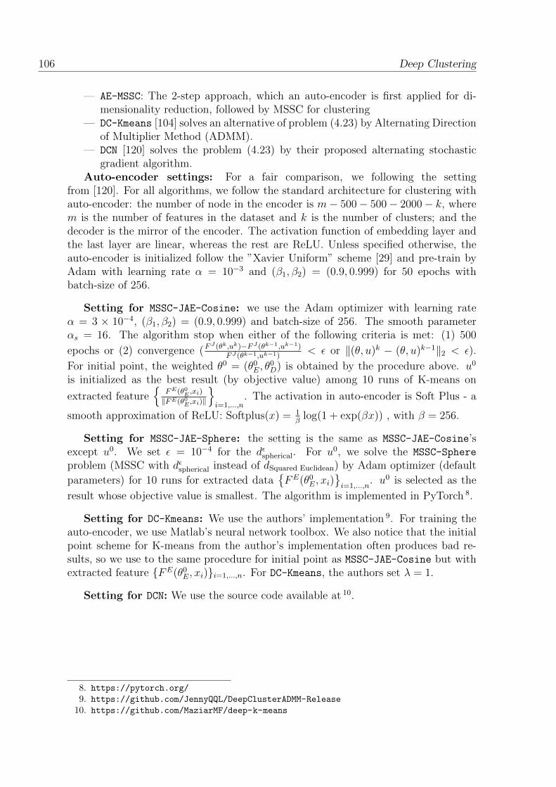
106 Deep Clustering
— AE-MSSC: The 2-step approach, which an auto-encoder is first applied for di-mensionality reduction, followed by MSSC for clustering
— DC-Kmeans [104] solves an alternative of problem (4.23) by Alternating Directionof Multiplier Method (ADMM).
— DCN [120] solves the problem (4.23) by their proposed alternating stochasticgradient algorithm.
Auto-encoder settings: For a fair comparison, we following the settingfrom [120]. For all algorithms, we follow the standard architecture for clustering withauto-encoder: the number of node in the encoder is m− 500− 500− 2000− k, wherem is the number of features in the dataset and k is the number of clusters; and thedecoder is the mirror of the encoder. The activation function of embedding layer andthe last layer are linear, whereas the rest are ReLU. Unless specified otherwise, theauto-encoder is initialized follow the ”Xavier Uniform” scheme [29] and pre-train byAdam with learning rate α = 10−3 and (β1, β2) = (0.9, 0.999) for 50 epochs withbatch-size of 256.
Setting for MSSC-JAE-Cosine: we use the Adam optimizer with learning rateα = 3 × 10⁻⁴, (β1, β2) = (0.9, 0.999) and batch-size of 256. The smooth parameterαs = 16. The algorithm stop when either of the following criteria is met: (1) 500
epochs or (2) convergence (FJ (θk,uk)−FJ (θk−1,uk−1)
FJ (θk−1,uk−1)< ε or ‖(θ, u)k − (θ, u)k−1‖2 < ε).
For initial point, the weighted θ0 = (θ0E, θ
0D) is obtained by the procedure above. u0
is initialized as the best result (by objective value) among 10 runs of K-means on
extracted feature
FE(θ0E ,xi)
‖FE(θ0E ,xi)‖
i=1,...,n
. The activation in auto-encoder is Soft Plus - a
smooth approximation of ReLU: Softplus(x) = 1β
log(1 + exp(βx)) , with β = 256.
Setting for MSSC-JAE-Sphere: the setting is the same as MSSC-JAE-Cosine’sexcept u0. We set ε = 10−4 for the dεspherical. For u0, we solve the MSSC-Sphere
problem (MSSC with dεspherical instead of dSquared Euclidean) by Adam optimizer (default
parameters) for 10 runs for extracted dataFE(θ0
E, xi)i=1,...,n
. u0 is selected as the
result whose objective value is smallest. The algorithm is implemented in PyTorch 8.
Setting for DC-Kmeans: We use the authors’ implementation 9. For training theauto-encoder, we use Matlab’s neural network toolbox. We also notice that the initialpoint scheme for K-means from the author’s implementation often produces bad re-sults, so we use to the same procedure for initial point as MSSC-JAE-Cosine but withextracted feature FE(θ0
E, xi)i=1,...,n. For DC-Kmeans, the authors set λ = 1.
Setting for DCN: We use the source code available at 10.
8. https://pytorch.org/
9. https://github.com/JennyQQL/DeepClusterADMM-Release
10. https://github.com/MaziarMF/deep-k-means
Deep Clustering 107
4.3.4.3 Experiment setting
Evaluation criteria: Given an input xi with ground-truth label li; and pi isthe assignment label from clustering algorithm, we measure the following criteria toevaluate experimental results:
— Clustering Accuracy (ACC [13]): ACC is calculated as ACC(l, p) =1n
∑ni=1 1m(pi)=li , where m(xi) is the function which maps each clustering as-
sign in pi to the equivalent label li. In our case, we use the mapping by usingthe Kuhn-Munkres algorithm [73].
— Normalized mutual information (NMI [102]): The NMI criterion is cal-
culated as NMI(l, p) = I(l,p)√H(l)H(p)
, where I(l, p) is the mutual information of l
and p.
All algorithms in our experiment (except MSSC and AE+KM) has a hyper parameterλ controls the trade-off between the auto-encoder and the clustering. For choosing theλ, we performs a grid search λ ∈ 10−7, 10−6, . . . , 102. We repeat the experiment 10times, select the results which has the highest accuracy among 10 runs, and report theaverage with standard deviation of each criterion.
All experiments are conducted on a Intel(R) Xeon (R) CPU E5-2630 v4 @2.20 GHzwith 32GB of RAM and a GTX 1080 GPU.
4.3.4.4 Experiment results
The experiment result of all datasets is reported in Table 4.3.
The results show that reducing the number of dimension by auto-encoder facilitatesthe clustering process: the increase in accuracy by using the 2-step approach (AE+MSSC)over clustering on raw data (MSSC) is significant. The gap in clustering accuracy is up to32.56% as in mnist dataset. However, the final result of both MSSC and AE+MSSC do notexceed the joint-clustering approach (DCN, MSSC-JAE-Cosine, and MSSC-JAE-Sphere).DCN further improves the accuracy of AE+MSSC among all 4 datasets, range from 0.33%to 2.68%.
The proposed methods (MSSC-JAE-Cosine and MSSC-JAE-Sphere) further improvethe clustering quality over DCN. The increase in terms of clustering accuracy is consis-tent, ranging from 1.21% to 7.63% (reps. from 2.48% to 8.17%) for MSSC-JAE-Cosine(reps. MSSC-JAE-Sphere). Both MSSC-JAE-Cosine and MSSC-JAE-Sphere pro-duces better results than DCN. The NMI of both results of MSSC-JAE-Cosine andMSSC-JAE-Sphere is higher than DCN’s, up to 3.90% and 6.72% respectively. Thisresult demonstrates the importance of regularization on the latent space, which isachieved in this case by projection the data point’s representation in the latent spaceonto the `2 ball. In addition, among two methods that utilize the `2 projection in thelatent space, MSSC-JAE-Sphere is undoubtedly better than MSSC-JAE-Cosine: thegap in clustering accuracy is from 0.22% (usps dataset) to 2.5% (mnist dataset). This
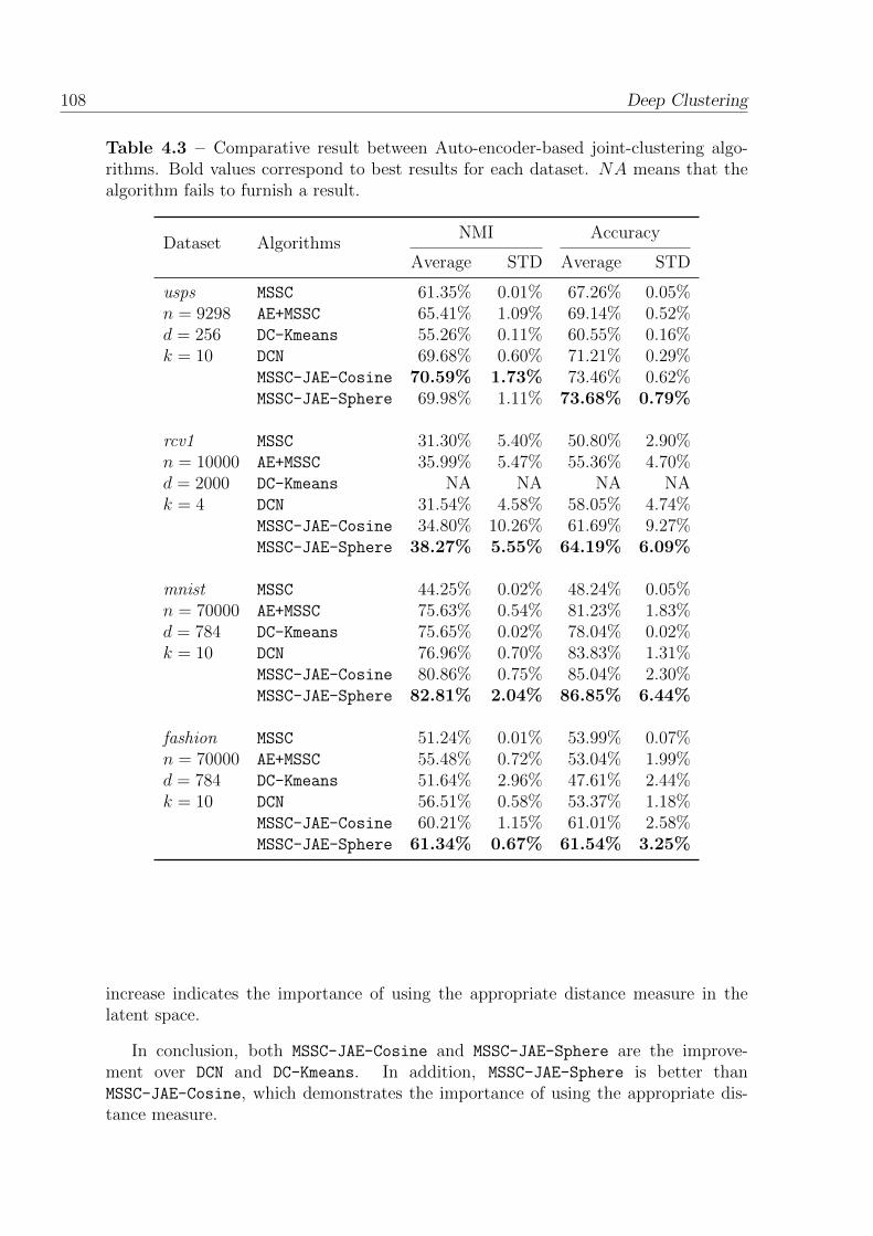
108 Deep Clustering
Table 4.3 – Comparative result between Auto-encoder-based joint-clustering algo-rithms. Bold values correspond to best results for each dataset. NA means that thealgorithm fails to furnish a result.
Dataset AlgorithmsNMI Accuracy
Average STD Average STD
usps MSSC 61.35% 0.01% 67.26% 0.05%n = 9298 AE+MSSC 65.41% 1.09% 69.14% 0.52%d = 256 DC-Kmeans 55.26% 0.11% 60.55% 0.16%k = 10 DCN 69.68% 0.60% 71.21% 0.29%
MSSC-JAE-Cosine 70.59% 1.73% 73.46% 0.62%MSSC-JAE-Sphere 69.98% 1.11% 73.68% 0.79%
rcv1 MSSC 31.30% 5.40% 50.80% 2.90%n = 10000 AE+MSSC 35.99% 5.47% 55.36% 4.70%d = 2000 DC-Kmeans NA NA NA NAk = 4 DCN 31.54% 4.58% 58.05% 4.74%
MSSC-JAE-Cosine 34.80% 10.26% 61.69% 9.27%MSSC-JAE-Sphere 38.27% 5.55% 64.19% 6.09%
mnist MSSC 44.25% 0.02% 48.24% 0.05%n = 70000 AE+MSSC 75.63% 0.54% 81.23% 1.83%d = 784 DC-Kmeans 75.65% 0.02% 78.04% 0.02%k = 10 DCN 76.96% 0.70% 83.83% 1.31%
MSSC-JAE-Cosine 80.86% 0.75% 85.04% 2.30%MSSC-JAE-Sphere 82.81% 2.04% 86.85% 6.44%
fashion MSSC 51.24% 0.01% 53.99% 0.07%n = 70000 AE+MSSC 55.48% 0.72% 53.04% 1.99%d = 784 DC-Kmeans 51.64% 2.96% 47.61% 2.44%k = 10 DCN 56.51% 0.58% 53.37% 1.18%
MSSC-JAE-Cosine 60.21% 1.15% 61.01% 2.58%MSSC-JAE-Sphere 61.34% 0.67% 61.54% 3.25%
increase indicates the importance of using the appropriate distance measure in thelatent space.
In conclusion, both MSSC-JAE-Cosine and MSSC-JAE-Sphere are the improve-ment over DCN and DC-Kmeans. In addition, MSSC-JAE-Sphere is better thanMSSC-JAE-Cosine, which demonstrates the importance of using the appropriate dis-tance measure.
Deep Clustering 109
4.4 Conclusion
In this chapter, we tackle the deep clustering problems in two directions. Thefirst direction considers the usage of t-SNE (t-Distributed Stochastic Neighbor Em-bedding) in clustering. We proposed two clustering methods for high-dimensionaldata based on DC Programming and DCA, named MSSC-2S and MSSC-JDR. MSSC-2Sis a straight-forward application of two high-efficiency DCA methods, Minimum Sum-of-Squares Clustering and t-SNE, where both have proved their effectiveness in theliterature. MSSC-JDR follows the joint-clustering approach to By exploiting the par-ticular structure of the problem, we have recast the joint-clustering problem as a DCprogram and proposed MSSC-JDR – a DCA-Like algorithm. MSSC-JDR solves two convexsub-problems at each iteration, both are relatively fast: one requires only elementaryoperations on vectors, the remaining one is solving a sparse linear system. Both meth-ods are applicable for many applications given an appropriate distance function. Thenumerical results show that the proposed methods significantly improve the cluster-ing quality in comparison with state-of-the-art methods in deep clustering, up to 38%higher than the second-best method. Furthermore, MSSC-JDR significantly reduces therunning time of MSSC-2S (up to 14 times) while having similar clustering accuracy. Weare convinced that the proposed methods are efficient, fast, and scalable for clusteringhigh-dimensional data.
The second direction considers joint-clustering using auto-encoder. We proposedan extension for deep joint-clustering problems by using cosine and spherical distancemeasure, which is applicable when the derived optimization problems suffer from thescaling of data’s representation in the latent space. Both distance measures are in-variance to scaling since they compute the distance between projections of data pointsonto the surface of the unit hypersphere Sm−1 instead of between the data points inRm. As an application, we considered the specific problem of deep joint-clusteringwith MSSC and proposed two algorithms (MSSC-JAE-Cosine and MSSC-JAE-Sphere)to solve the mentioned problem. The numerical results present the effectiveness ofproposed algorithms in comparison with state-of-the-art methods in joint-clusteringby K-means. The clustering accuracy is higher in comparison with the second-bestmethod (from 3.90% to 6.72%). In addition, MSSC-JAE-Sphere improves the cluster-ing accuracy MSSC-JAE-Cosine by up to 2.5%, which indicates the importance of usingthe appropriate distance measure in the latent space.
Each developed method has its advantages and disadvantages. The first method –clustering based on t-SNE – works well in case we can define a distance function tomeasure the similarity between data-points in the original space. On the other hand,since the second approach based on the auto-encoder, it seeks the mapping functionsolely based on input data, hence eliminating the needs of the similarity function.However, the auto-encoder-based approach requires a massive amount of data to workwell, so in case we can gather or generate data [32], this is a preferable choice. Hence,the choice is the trade-off between expert knowledge and data-driven approach: howcan we define the similarity function versus the amount of the data we have.
110 Deep Clustering
In conclusion, the proposed methods have demonstrated their effectiveness in bothterms of clustering accuracy and running time in comparison to the relevance methods.In the future, we could extend MSSC-JAE-Sphere to consider other unit spheres otherthan `2 such as `p ball (p ∈ 1,∞). On another direction, we could consider thecombination between t-SNE and neural network for deep joint-clustering problems.MSSC-JDR based on t-SNE is better than MSSC-JAE-Sphere in clustering accuracy,nevertheless, MSSC-JDR requires a distance measure to capture the similarity betweendata points in the original whereas MSSC-JAE-Sphere does not need. The combinationbetween them is interesting since it could take the advantages from both methods.

Chapter 5
Conclusion
This dissertation focus on three problems in machine learning on big data: groupvariable selection in multi-class logistic regression, dimension reduction by t-SNE anddeep clustering. The principal methodologies of this dissertation are DC (Differenceof Convex functions) programming and DCA (DC Algorithm) and their advancedvariances, which are well-known powerful tools due to their effectiveness and efficiencyfor non-smooth and non-convex optimization problems.
The first part rigorously studied the DC programming and DCA for the problem ofgroup variables selection in multi-class logistic regression. Using the `q,0 regularization,the resulting optimization problem is non-convex. The `q,0-norm is approximated bythe piecewise exponential function and the capped-`1 function. We studied DCA forthis problem and developed DCA-based algorithms to solve the approximated problemby two approaches based on recent advanced DC algorithms. The proposed algorithmin the first approach, SDCA, is based on Stochastic DCA. SDCA is very inexpensive andsuitable for large-scale datasets. In the second approach, we developed two algorithmsbased on DCA-Like and its accelerated version ADCA-Like. Both algorithms extendDCA by relaxing the DCA’s convexity condition on the second DC component, whilestill ensuring the convergence. Unlike standard DCA where we need to compute theparameter µ greater or equal to the L-Lipschitz constant, which is difficult (or even im-possible) in practice; DCA-Like iteratively updates the parameter µ and consequentlythe decomposition of the objective function. The proposed algorithms are efficient: allcomputations are explicit.
The numerical experiments have shown that all proposed algorithms significantlyimprove the running time in comparison with standard DCA while having equivalentclassification accuracy and sparsity. They also give better results than the relatedalgorithms in the literature in both terms of classification accuracy and running time.Among the proposed algorithms, choosing an appropriate algorithm depends on thedataset’s size and the number of the selected variables. SDCA is more suitable for largedatasets, whereas ADCA-Like and DCA-Like are ideal if we prefer a more compactsubset of variables. We are convinced that proposed algorithms are efficient for theproblem of group variable selection in multi-class logistic regression.
111

112 Conclusion
In the second part, we studied DC programming and DCA for the t-SNE prob-lem. The two proposed algorithms are based on DCA-Like and ADCA-Like, whichare inexpensive: the solution of the convex sub-problem can be explicitly computed.We showed that the Majorization-Minimization algorithm, the best state-of-the-artalgorithm for t-SNE is nothing else but DCA-Like applied for t-SNE. Numerical ex-periments were carefully conducted on several benchmark datasets for visualization.The numerical results show that DCA-Like dramatically improves the running timeof standard DCA while giving a similar or better solution. Besides, ADCA-Likes im-proves further the running time as well as the objective value of DCA-Like. Thus, wecan conclude that the two proposed methods are the best for the t-SNE problem.
Finally, the last part tackles the deep clustering problems in two directions. Thefirst direction considered the usage of t-SNE in clustering for large-scale datasets.Two algorithms based on DC Programming and DCA, MSSC-2S and MSSC-JDR, havebeen developed. MSSC-2S follows the standard “tandem analysis” by employing twowell-performance DCAs (for t-SNE and MSSC), whereas MSSC-JDR is an extension ofMSSC-2S by following the joint-clustering approach. We developed a fast and scalableDCA-Like algorithm for MSSC-JDR. The numerical results show that both methods sig-nificantly improve the clustering quality and running time in comparison with existingmethods. Furthermore, MSSC-JDR significantly reduces the running time of MSSC-2S
while having similar accuracy. Hence, our methods are efficient, fast and scalablefor clustering large-scale data. The second direction considers the problem of joint-clustering with auto-encoder. We considered a class of methods that suffers from thescaling problem in latent space; and proposed an extension by employing the cosinedistance and spherical distance, which are invariance to scaling. We applied the pro-posed extension on a specific problem of joint-clustering with MSSC. The numericalresults show the superiority of our methods in comparison with existing methods.
Each developed clustering method has its advantages and disadvantages. The maindistinction between them are based on the distance function measures the similarityof data points in the original space. The first method – clustering based on t-SNE –works well in case we can define such function; whereas the second method – based onauto-encoder – eliminates that requirement. However, the auto-encoder-based methodrequires a massive amount to learn a good mapping function, so it is preferable if wecan gather a huge volume of data or generate more data [32]. Hence, the choice is thetrade-off between expert knowledge and data-driven approach: how can we define thedistance function versus the amount of the data we have.
The works in this dissertation raise the following topics that can be consideredin the near future. In terms of modeling, for the deep clustering problem, we couldextend MSSC-JAE-Sphere to consider other unit spheres other than `2 such as `p ball(p ∈ 1,∞). On another direction, we could consider the combination betweent-SNE and neural network for deep joint-clustering problems. MSSC-JDR based on t-SNE is better than MSSC-JAE-Sphere in clustering accuracy. Nevertheless, MSSC-JDRrequires a distance measure to capture the similarity between data points in the orig-inal, whereas MSSC-JAE-Sphere does not need since the reconstruction error in theauto-encoder does not require external information. The combination between them is

Conclusion 113
interesting since it could take advantages of both methods. Furthermore, [32] considersdata augmentation in deep clustering improves the accuracy of the based model signif-icantly. This technique further exploits the self-supervised nature of the auto-encoder,which is a promising research direction for deep clustering. In terms of optimization,it is possible to develop DCAs for the neural network in general, and deep clusteringproblem in particular.

114 Conclusion

Appendix A
Appendix
A.1 Computation of prox(−zlj)/ρ‖.‖q(ν/ρ)
Denote by Bq the unit ball for the dual norm of the `q norm. By Moreau decom-position, we have
prox(−zlj)/ρ‖.‖q(ν/ρ) = ν/ρ− (−zlj)/ρprojBq
(1
−zljν
), (A.1)
where projBq denotes the projection onto Bq and is computed as follows.
For q = 1, the unit ball of the `1 norm is the box B1 = x : ‖x‖1 ≤ 1. Hence, theprojection onto this box is given by
projB1
(1
−zljν
)k
=
1 if 1
−zljνk > 1
1−zlj
νk if | 1−zlj
νk| ≤ 1
−1 if 1−zlj
νk < −1.
(A.2)
From (A.1) and (A.2), we obtain
prox(−zlj)/ρ‖.‖q(ν/ρ)k =
νk/ρ− (−zlj)/ρ if νk > −zlj0 if |νk| ≤ −zljνk/ρ+ (−zlj)/ρ if νk < zlj.
This is also known as the elementwise soft thresholding given by
prox(−zlj)/ρ‖.‖q(ν/ρ) =
(|ν|/ρ− (−zlj)/ρ
)+ sign(ν),
where is the elementwise product.
115
116 Appendix
For q = 2, the unit ball of the `2 norm is the Euclidean unit ball B2 = x : ‖x‖2 ≤1. Hence, the projection onto this ball is given by
projB2
(1
−zljν
)=
ν‖ν‖2 if 1
−zlj‖ν‖2 > 1
1−zlj
ν if 1−zlj‖ν‖2 ≤ 1.
(A.3)
It follows from (A.1) and (A.3) that
prox(−zlj)/ρ‖.‖q(ν/ρ) =
(1− −zlj
‖ν‖2
)ν/ρ if ‖ν‖2 > −zlj
0 if ‖ν‖2 ≤ −zlj.
For q =∞, the unit ball of the `∞ norm is the ball B∞ = x : ‖x‖∞ ≤ 1. Hence,the projection onto this ball is given by
projB∞
(1
−zljν
)=
(
1−zlj|ν| − δ
)+ sign(ν) if 1
−zlj‖ν‖1 > 1
1−zlj
ν if 1−zlja‖ν‖1 ≤ 1,
(A.4)
where δ satisfies the following equation
Q∑k=1
(1
−zlj|νk| − δ
)+
= 1. (A.5)
For computing δ in (A.5), some efficient algorithms are available. Among them, weuse the very inexpensive algorithm developed in [25]. From (A.1) and (A.4), we get
prox(−zlj)/ρ‖.‖q(ν/ρ) =
ν/ρ−(
1−zlj|ν| − δ
)+ sign(ν) if ‖ν‖1 > −zlj
0 if ‖ν‖1 ≤ −zlj.
A.2 Solving problem (4.13) by first order optimality
condition
The sub-problem (4.13) is a convex problem. Hence, we can effectively obtain thesolution by solving the system of equation ∇FS(u, z) = 0. It leads to
0 = ∇uGC(u, z)− uCq (A.6)
0 = λ(∇zGC(u, z)− zCq) + µz − zEq +∇z
(∑i,j
(−vEqij)gij(z)
)(A.7)
By expanding both (A.6) and (A.7), we obtained the following solution:
Eq (A.6) ⇔ nu− 1k×nz = uCq
⇔ u =1
n(uC
q + 1k×nz) (A.8)

Appendix 117
Expanding Eq (A.7)
⇔ λ(∇zGC(u, z)− zCq) + µz − zEq +∇z
(∑i,j
(−vEqij)‖zi − zj‖2
)= 0
⇔ λ(kz − 1n×ku− zCq) + µz − zEq + 2(L−vEq−(vEq)T )z = 0
⇔ λ(kz − 1n×ku) + µz + 2(L−vEq−(vEq)T )z = λzCq + zE
q
⇔((λk + µ)In + 2(L−vEq−(vEq)T )
)z − λ1n×ku = λzC
q + zEq
(A.8)⇔((λk + µ)In + 2(L−vEq−(vEq)T )
)z − λ
n1n×k (uC
q + 1k×nz) = λzCq + zE
q
⇔((λk + µ)In + 2(L−vEq−(vEq)T )
)z − λk
n1n×nz = λzC
q + zEq +
λ
n1n×kuC
q
⇔(λk
(In −
1
n1n×n
)+ 2(L−vEq−(vEq)T ) + µIn
)z = λzC
q + zEq +
λ
n1n×kuC
q
⇔
(λk + µ)In + 2(L−vEq−(vEq)T )︸ ︷︷ ︸Aq
− λkn1n×n︸ ︷︷ ︸Bq
z = λzCq + zE
q +λ
n1n×kuC
q︸ ︷︷ ︸Cq
⇔ (Aq − Bq)z = Cq (A.9)
A.3 Solving convex sub-problem (4.17)
Let FS2(z) denotes objective function of problem (4.17). Since the problem (4.17)is convex, then by applying the first order optimality condition, we can obtained thesolution by solving ∇FS2(z) = 0, which is equivalent to
⇔ λ(∇zGC(uq,t, z)− zCq) + µz − zEq +∇z
(∑i,j
(−vEqij)gij(z)
)= 0
⇔ λ(kz − 1n×kuq,t) + µz + 2(L−vEq−(vEq)T )z = λzC
q + zEq
⇔ λkz + µz + 2(L−vEq−(vEq)T )z = λzCq + zE
q + λ1n×kuq,t
⇔((λk + µ)In + 2(L−vEq−(vEq)T )
)z = λzC
q + zEq + λ1n×ku
q,t
(A.10)

118 Appendix

Bibliography
[1] Aghabozorgi, S., Seyed Shirkhorshidi, A., and Ying Wah, T. (2015). Time-seriesclustering – A decade review. Information Systems, 53:16–38.
[2] Aljalbout, E., Golkov, V., Siddiqui, Y., and Cremers, D. (2018). Clustering withDeep Learning: Taxonomy and New Methods. arXiv:1801.07648 [cs, stat].
[3] Amaldi, E. and Kann, V. (1998). On the approximability of minimizing nonzerovariables or unsatisfied relations in linear systems. Theor. Comput. Sci., 209(1):237–260.
[4] An(Homepage), L. T. H. (2005). DC Programming and DCA:http://www.lita.univ-lorraine.fr/~lethi/index.php/en/research/
dc-programming-and-dca.html.
[5] Aytekin, C., Ni, X., Cricri, F., and Aksu, E. (2018). Clustering and Unsuper-vised Anomaly Detection with `2 Normalized Deep Auto-Encoder Representations.arXiv:1802.00187 [cs].
[6] Bagley, S. C., White, H., and Golomb, B. A. (2001). Logistic regression in themedical literature: Standards for use and reporting, with particular attention toone medical domain. Journal of Clinical Epidemiology, 54(10):979–985.
[7] Bagozzi, R. P. (1994). Advanced Methods of Marketing Research. Blackwell Busi-ness.
[8] Boyd, C. R., Tolson, M. A., and Copes, W. S. (1987). Evaluating trauma care:The TRISS method. Trauma Score and the Injury Severity Score. The Journal ofTrauma, 27(4):370–378.
[9] Boyd, S. and Vandenberghe, L. (2004). Convex Optimization. Cambridge universitypress.
[10] Bradley, P. S. and Mangasarian, O. L. (1998a). Feature selection via concaveminimization and support vector machines. In ICML, volume 98, pages 82–90.
[11] Bradley, P. S. and Mangasarian, O. L. (1998b). Feature selection via concaveminimization and support vector machines. In Machine Learning Proceedings of theFifteenth International Conference (ICML 1998), pages 82–90. Morgan Kaufmann.
119
120 Bibliography
[12] Burges, C. J. C. (2009). Dimension Reduction: A Guided Tour. FNT in MachineLearning, 2(4):275–364.
[13] Cai, D., He, X., and Han, J. (2011). Locally Consistent Concept Factorizationfor Document Clustering. IEEE Transactions on Knowledge and Data Engineering,23(6):902–913.
[14] Caron, M., Bojanowski, P., Joulin, A., and Douze, M. (2018). Deep Clusteringfor Unsupervised Learning of Visual Features. In Ferrari, V., Hebert, M., Sminchis-escu, C., and Weiss, Y., editors, Computer Vision – ECCV 2018, Lecture Notes inComputer Science, pages 139–156. Springer International Publishing.
[15] Chambolle, A., Vore, R. A. D., Nam-Yong Lee, and Lucier, B. J. (1998). Nonlinearwavelet image processing: Variational problems, compression, and noise removalthrough wavelet shrinkage. IEEE Transactions on Image Processing, 7(3):319–335.
[16] Chang, W.-C. (1983). On Using Principal Components Before Separating a Mix-ture of Two Multivariate Normal Distributions. Journal of the Royal StatisticalSociety. Series C (Applied Statistics), 32(3):267–275.
[17] Chen, D., Lv, J., and Zhang, Y. (2017). Unsupervised Multi-Manifold Clusteringby Learning Deep Representation. In Workshops at the Thirty-First AAAI Confer-ence on Artificial Intelligence.
[18] Collobert, R., Sinz, F., Weston, J., and Bottou, L. (2006). Trading convexity forscalability. In In ICML ’06: Proceedings of the 23rd International Conference onMachine Learning, pages 201–208. ACM Press.
[19] Cox, D. (1958). The regression analysis of binary sequences (with discussion). JRoy Stat Soc B, 20:215–242.
[20] Da Silva, G., Le, H. M., Le Thi, H. A., Lefieux, V., and Tran, B. (2020). Cus-tomer Clustering of French Transmission System Operator (RTE) Based on TheirElectricity Consumption. In Le Thi, H. A., Le, H. M., and Pham Dinh, T., editors,Optimization of Complex Systems: Theory, Models, Algorithms and Applications,Advances in Intelligent Systems and Computing, pages 893–905. Springer Interna-tional Publishing.
[21] Das, D., Ghosh, R., and Bhowmick, B. (2019). Deep Representation LearningCharacterized by Inter-Class Separation for Image Clustering. In 2019 IEEE WinterConference on Applications of Computer Vision (WACV), pages 628–637.
[22] De Soete, G. and Carroll, J. D. (1994). K-means clustering in a low-dimensionalEuclidean space. In Diday, E., Lechevallier, Y., Schader, M., Bertrand, P., andBurtschy, B., editors, New Approaches in Classification and Data Analysis, Stud-ies in Classification, Data Analysis, and Knowledge Organization, pages 212–219.Springer Berlin Heidelberg.

Bibliography 121
[23] Dempster, A. P., Laird, N. M., and Rubin, D. B. (1977). Maximum Likelihoodfrom Incomplete Data Via the EM Algorithm. Journal of the Royal StatisticalSociety: Series B (Methodological), 39(1):1–22.
[24] Dhillon, I. S. and Modha, D. S. (2001). Concept Decompositions for Large SparseText Data Using Clustering. Machine Learning, 42(1):143–175.
[25] Duchi, J., Shalev-Shwartz, S., Singer, Y., and Chandra, T. (2008). Efficientprojections onto the l 1-ball for learning in high dimensions. In Proceedings of the25th International Conference on Machine Learning, pages 272–279. ACM.
[26] Fard, M. M., Thonet, T., and Gaussier, E. (2018). Deep k-Means: Jointly clus-tering with k-Means and learning representations. arXiv:1806.10069 [cs, stat].
[27] Genkin, A., Lewis, D. D., and Madigan, D. (2007). Large-scale Bayesian logisticregression for text categorization. Technometrics, 49(3):291–304.
[28] Ghasedi Dizaji, K., Herandi, A., Deng, C., Cai, W., and Huang, H. (2017). Deepclustering via joint convolutional autoencoder embedding and relative entropy mini-mization. In Proceedings of the IEEE International Conference on Computer Vision,pages 5736–5745.
[29] Glorot, X. and Bengio, Y. (2010). Understanding the difficulty of training deepfeedforward neural networks. In Proceedings of the Thirteenth International Con-ference on Artificial Intelligence and Statistics, pages 249–256.
[30] Goldin, D. Q. and Kanellakis, P. C. (1995). On similarity queries for time-seriesdata: Constraint specification and implementation. In Montanari, U. and Rossi,F., editors, Principles and Practice of Constraint Programming — CP ’95, LectureNotes in Computer Science, pages 137–153. Springer Berlin Heidelberg.
[31] Goodfellow, I., Bengio, Y., and Courville, A. (2016). Deep Learning. MIT Press.
[32] Guo, X. (2018). Deep Embedded Clustering with Data Augmentation. In ACML,page 16.
[33] Guo, X., Gao, L., Liu, X., and Yin, J. (2017). Improved deep embedded clusteringwith local structure preservation. In International Joint Conference on ArtificialIntelligence (IJCAI-17), pages 1753–1759.
[34] Hinton, G. E. and Roweis, S. T. (2003). Stochastic neighbor embedding. InAdvances in Neural Information Processing Systems, pages 857–864.
[35] Hinton, G. E. and Salakhutdinov, R. R. (2006). Reducing the Dimensionality ofData with Neural Networks. Science, 313(5786):504–507.
[36] Hiriart-Urruty, J.-B. and Lemarechal, C. (1993). Convex Analysis and Mini-mization Algorithms. Grundlehren Der Mathematischen Wissenschaften, ConvexAnalysis and Minimization Algorithms. Springer-Verlag, Berlin Heidelberg.
122 Bibliography
[37] Huang, P., Huang, Y., Wang, W., and Wang, L. (2014). Deep Embedding Networkfor Clustering. In 2014 22nd International Conference on Pattern Recognition, pages1532–1537.
[38] Ji, P., Zhang, T., Li, H., Salzmann, M., and Reid, I. (2017). Deep SubspaceClustering Networks. In NIPS.
[39] Kim, J., Kim, Y., and Kim, Y. (2008). A Gradient-Based Optimization Algorithmfor LASSO. Journal of Computational and Graphical Statistics, 17(4):994–1009.
[40] King, G. and Zeng, L. (2001). Logistic Regression in Rare Events Data. PoliticalAnalysis, 9:137–163.
[41] Kingma, D. P. and Ba, J. (2014). Adam: A Method for Stochastic Optimization.arXiv:1412.6980 [cs].
[42] Le, H. M., Le Thi, H. A., and Nguyen, M. C. (2015). Sparse semi-supervisedsupport vector machines by DC programming and DCA. Neurocomputing, 153:62–76.
[43] Le Tan, D.-K., Le, H., Hoang, T., Do, T.-T., and Cheung, N.-M. (2018). DeepVQ:A deep network architecture for vector quantization. In Proceedings of the IEEEConference on Computer Vision and Pattern Recognition Workshops, pages 2579–2582.
[44] Le Thi, H. A. (1997). Contribution a l’optimisation non convexe et l’optimisationglobale: Theorie, algorithmes et applications. Habilitation a Diriger des Recherches,Universite de Rouen.
[45] Le Thi, H. A., Belghiti, M. T., and Pham Dinh, T. (2007). A new efficientalgorithm based on DC programming and DCA for clustering. Journal of GlobalOptimization, 37(4):593–608.
[46] Le Thi, H. A., Le, H. M., Nguyen, V. V., and Pham Dinh, T. (2008). A DCprogramming approach for feature selection in support vector machines learning.Advances in Data Analysis and Classification, 2(3):259–278.
[47] Le Thi, H. A., Le, H. M., and Pham Dinh, T. (2014a). New and efficientDCA based algorithms for minimum sum-of-squares clustering. Pattern Recogni-tion, 47(1):388–401.
[48] Le Thi, H. A., Le, H. M., and Pham Dinh, T. (2015a). Feature selection inmachine learning: An exact penalty approach using a Difference of Convex functionAlgorithm. Mach Learn, 101(1):163–186.
[49] Le Thi, H. A., Le, H. M., Pham Dinh, T., and Van Huynh, N. (2013). Binaryclassification via spherical separator by DC programming and DCA. J Glob Optim,56(4):1393–1407.
Bibliography 123
[50] Le Thi, H. A., Le, H. M., Phan, D. N., and Tran, B. (2017). Stochastic DCA for theLarge-sum of Non-convex Functions Problem and its Application to Group VariableSelection in Classification. In Proceedings of the 34th International Conference onMachine Learning , volume 70, pages 3394–3403.
[51] Le Thi, H. A., Le, H. M., Phan, D. N., and Tran, B. (2018a). A DCA-LikeAlgorithm and its Accelerated Version with Application in Data Visualization. InarXiv:1806.09620 [Cs, Math].
[52] Le Thi, H. A., Le, H. M., Phan, D. N., and Tran, B. (2018b). Stochastic DCA forsparse multiclass logistic regression. In Le, N.-T., van Do, T., Nguyen, N. T., andLe Thi, H. A., editors, Advanced Computational Methods for Knowledge Engineering,pages 1–12.
[53] Le Thi, H. A., Le, H. M., Phan, D. N., and Tran, B. (2019a). Novel DCABased Algorithms for Minimizing the Sum of a Nonconvex Function and Compos-ite Functions. Applications in Machine learning. Submitted & Available on arvXiv[arXiv:1806.09620].
[54] Le Thi, H. A., Le, H. M., Phan, D. N., and Tran, B. (2019b). Stochastic DCAfor minimizing a large sum of DC functions with application to Multi-class LogisticRegression. Submitted & Available on arvXiv [arXiv:1911.03992].
[55] Le Thi, H. A. and Moeini, M. (2014). Long-Short Portfolio Optimization UnderCardinality Constraints by Difference of Convex Functions Algorithm. J OptimTheory Appl, 161(1):199–224.
[56] Le Thi, H. A. and Nguyen, M. C. (2014). Self-organizing maps by difference ofconvex functions optimization. Data Min Knowl Disc, 28(5):1336–1365.
[57] Le Thi, H. A. and Nguyen, M. C. (2017). DCA based algorithms for featureselection in multi-class support vector machine. Ann Oper Res, 249(1):273–300.
[58] Le Thi, H. A., Nguyen, M. C., and Pham Dinh, T. (2014b). A DC ProgrammingApproach for Finding Communities in Networks. Neural Computation, 26(12):2827–2854.
[59] Le Thi, H. A. and Pham Dinh, T. (1997). Solving a Class of Linearly ConstrainedIndefinite Quadratic Problems by D.C. Algorithms. Journal of Global Optimization,11(3):253–285.
[60] Le Thi, H. A. and Pham Dinh, T. (2005). The DC (Difference of Convex Func-tions) Programming and DCA Revisited with DC Models of Real World NonconvexOptimization Problems. Annals of Operations Research, 133(1):23–46.
[61] Le Thi, H. A. and Pham Dinh, T. (2009). Minimum sum-of-squares clustering byDC programming and DCA. In International Conference on Intelligent Computing,pages 327–340. Springer.
124 Bibliography
[62] Le Thi, H. A. and Pham Dinh, T. (2018). DC programming and DCA: thirtyyears of developments. Mathematical Programming, pages 1–64.
[63] Le Thi, H. A., Pham Dinh, T., Le, H. M., and Vo, X. T. (2015b). DC approxima-tion approaches for sparse optimization. European Journal of Operational Research,244(1):26–46.
[64] Le Thi, H. A., Pham Dinh, T., and Thiao, M. (2016a). Efficient approaches for `2-`0 regularization and applications to feature selection in SVM. Applied Intelligence,45(2):549 – 565.
[65] Le Thi, H. A. and Phan, D. N. (2016). DC Programming and DCA for SparseOptimal Scoring Problem. Neurocomput., 186(C):170–181.
[66] Le Thi, H. A. and Phan, D. N. (2017). DC Programming and DCA for SparseFisher Linear Discriminant Analysis. Neural Comput. Appl., 28(9):2809–2822.
[67] Le Thi, H. A., Vo, X. T., and Pham Dinh, T. (2016b). Efficient NonnegativeMatrix Factorization by DC Programming and DCA. Neural Comput, 28(6):1163–1216.
[68] Lecun, Y., Bottou, L., Bengio, Y., and Haffner, P. (1998). Gradient-based learningapplied to document recognition. Proceedings of the IEEE, 86(11):2278–2324.
[69] Li, H. and Lin, Z. (2015). Accelerated proximal gradient methods for nonconvexprogramming. In Advances in Neural Information Processing Systems, pages 377–387.
[70] Liao, J. G. and Chin, K.-V. (2007). Logistic regression for disease classificationusing microarray data: Model selection in a large p and small n case. Bioinformatics,23(15):1945–1951.
[71] Liu, Y. and Shen, X. (2006). Multicategory ψ-Learning. Journal of the AmericanStatistical Association, 101(474):500–509.
[72] Lloyd, S. (1982). Least squares quantization in PCM. IEEE Transactions onInformation Theory, 28(2):129–137.
[73] Lovasz, L. and Plummer, M. D. (2009). Matching Theory. American MathematicalSoc.
[74] Maaten, L. v. d. (2014). Accelerating t-sne using tree-based algorithms. Journalof machine learning research, 15(1):3221–3245.
[75] MacQueen, J. (1967). Some methods for classification and analysis of multivari-ate observations. In Proceedings of the Fifth Berkeley Symposium on MathematicalStatistics and Probability, Volume 1: Statistics, pages 281–297. The Regents of theUniversity of California.
Bibliography 125
[76] Min, E., Guo, X., Liu, Q., Zhang, G., Cui, J., and Long, J. (2018). A Surveyof Clustering With Deep Learning: From the Perspective of Network Architecture.IEEE Access, 6:39501–39514.
[77] Mnih, V., Kavukcuoglu, K., Silver, D., Rusu, A. A., Veness, J., Bellemare, M. G.,Graves, A., Riedmiller, M., Fidjeland, A. K., Ostrovski, G., Petersen, S., Beattie, C.,Sadik, A., Antonoglou, I., King, H., Kumaran, D., Wierstra, D., Legg, S., and Has-sabis, D. (2015). Human-level control through deep reinforcement learning. Nature,518(7540):529–533.
[78] Mori, Y., Kuroda, M., and Makino, N. (2016). Joint Dimension Reduction andClustering. In Mori, Y., Kuroda, M., and Makino, N., editors, Nonlinear PrincipalComponent Analysis and Its Applications, SpringerBriefs in Statistics, pages 57–64.Springer Singapore, Singapore.
[79] Nair, V. and Hinton, G. E. (2010). Rectified Linear Units Improve RestrictedBoltzmann Machines. In Proceedings of the 27th International Conference on Inter-national Conference on Machine Learning, ICML’10, pages 807–814, USA. Omni-press.
[80] Nguyen, T. M. T. (2018). DCA Based Approaches for Mathematical Programswith Equilibrium Constraints. PhD thesis, Universite de Lorraine.
[81] Nocedal, J. (1980). Updating Quasi-Newton Matrices with Limited Storage. Math-ematics of Computation, 35(151):773–782.
[82] Paparrizos, J. and Gravano, L. (2015). K-Shape: Efficient and Accurate Clus-tering of Time Series. In Proceedings of the 2015 ACM SIGMOD InternationalConference on Management of Data, pages 1855–1870. ACM Press.
[83] Parikh, N. and Boyd, S. (2014). Proximal algorithms. Found. Trends Optim.,1(3):127–239.
[84] Pham Dinh, T., Le, H. M., Le Thi, H. A., and Lauer, F. (2014). A Difference ofConvex Functions Algorithm for Switched Linear Regression. IEEE Transactionson Automatic Control, 59(8):2277–2282.
[85] Pham Dinh, T. and Le Thi, H. A. (1997). Convex analysis approach to dc pro-gramming: Theory, algorithms and applications. Acta Mathematica Vietnamica,22(1):289–355.
[86] Pham Dinh, T. and Le Thi, H. A. (1998). A D. C. Optimization Algorithm forSolving the Trust-Region Subproblem. SIAM Journal of Optimization, 8(2):476–505.
[87] Pham Dinh, T. and Le Thi, H. A. (2014). Recent Advances in DC Programmingand DCA. In Nguyen, N. T. and Le Thi, H. A., editors, Transactions on Compu-tational Intelligence XIII, Lecture Notes in Computer Science, pages 1–37. SpringerBerlin Heidelberg.
126 Bibliography
[88] Pham Dinh, T. and Souad, E. B. (1986). Algorithms for Solving a Class ofNonconvex Optimization Problems. Methods of Subgradients. In Hiriart-Urruty,J. B., editor, North-Holland Mathematics Studies, volume 129 of Fermat Days 85:Mathematics for Optimization, pages 249–271. North-Holland.
[89] Phan, D. N., Le, H. M., and Le Thi, H. A. (2018). Accelerated Difference of Con-vex functions Algorithm and its Application to Sparse Binary Logistic Regression.In Twenty-Seventh International Joint Conference on Artificial Intelligence, pages1369–1375.
[90] Phan, D. N., Le Thi, H. A., and Pham Dinh, T. (2017). Sparse covariance matrixestimation by DCA-Based Algorithms. Neural Computation, 29(11):3040–3077.
[91] Rakotomamonjy, A., Flamary, R., and Gasso, G. (2016). DC Proximal Newtonfor Nonconvex Optimization Problems. IEEE Transactions on Neural Networks andLearning Systems, 27(3):636–647.
[92] Rakthanmanon, T., Campana, B., Mueen, A., Batista, G., Westover, B., Zhu, Q.,Zakaria, J., and Keogh, E. (2012). Searching and mining trillions of time series sub-sequences under dynamic time warping. In Proceedings of the 18th ACM SIGKDDInternational Conference on Knowledge Discovery and Data Mining - KDD ’12,page 262, Beijing, China. ACM Press.
[93] Rockafellar, R. T. (1970). Convex Analysis. Princeton, NJ.
[94] Rogovschi, N., Kitazono, J., Grozavu, N., Omori, T., and Ozawa, S. (2017). T-Distributed stochastic neighbor embedding spectral clustering. In 2017 InternationalJoint Conference on Neural Networks (IJCNN), pages 1628–1632.
[95] Rumelhart, D. E., Hinton, G. E., and Williams, R. J. (1986). Learning represen-tations by back-propagating errors. Nature, 323(6088):533.
[96] Shah, S. A. and Koltun, V. (2018). Deep Continuous Clustering. arXiv:1803.01449[cs].
[97] Shaol, X., Ge, K., Su, H., Luo, L., Peng, B., and Li, D. (2018). Deep Discrimina-tive Clustering Network. In 2018 International Joint Conference on Neural Networks(IJCNN), pages 1–7, Rio de Janeiro. IEEE.
[98] Shewchuk, J. R. (1994). An Introduction to the Conjugate Gradient MethodWithout the Agonizing Pain. Technical report, Carnegie Mellon University, Pitts-burgh, PA, USA.
[99] Song, C., Liu, F., Huang, Y., Wang, L., and Tan, T. (2013). Auto-encoder BasedData Clustering. In Progress in Pattern Recognition, Image Analysis, Computer Vi-sion, and Applications, Lecture Notes in Computer Science, pages 117–124. Springer,Berlin, Heidelberg.
[100] Souvenir, R. and Pless, R. (2005). Manifold clustering. In Tenth IEEE Interna-tional Conference on Computer Vision (ICCV’05) Volume 1, pages 648–653 Vol. 1,Beijing, China. IEEE.

Bibliography 127
[101] Steinbach, M., Ertoz, L., and Kumar, V. (2004). The Challenges of ClusteringHigh Dimensional Data. In Wille, L. T., editor, New Directions in Statistical Physics:Econophysics, Bioinformatics, and Pattern Recognition, pages 273–309. SpringerBerlin Heidelberg, Berlin, Heidelberg.
[102] Strehl, A. and Ghosh, J. (2002). Cluster Ensembles - A Knowledge Reuse Frame-work for Combining Multiple Partitions. Journal of Machine Learning Research,3:583–617.
[103] Subasi, A. and Ercelebi, E. (2005). Classification of EEG signals using neuralnetwork and logistic regression. Comput. Methods Programs Biomed., 78(2):87–99.
[104] Tian, K., Zhou, S., and Guan, J. (2017). DeepCluster: A General ClusteringFramework Based on Deep Learning. In Joint European Conference on MachineLearning and Knowledge Discovery in Databases, pages 809–825. Springer.
[105] Van Der Maaten, L. (2009). Learning a parametric embedding by preservinglocal structure. RBM, 500(500):26.
[106] van der Maaten, L. and Hinton, G. (2008). Visualizing Data using t-SNE. Journalof Machine Learning Research, 9(Nov):2579–2605.
[107] Van Der Maaten, L., Postma, E., and Van den Herik, J. (2009). DimensionalityReduction: A Comparative Review. J Mach Learn Res, 10(66-71):13.
[108] Vichi, M. and Kiers, H. A. (2001). Factorial k-means analysis for two-way data.Computational Statistics & Data Analysis, 37(1):49–64.
[109] Vincent, M. and Hansen, N. R. (2014). Sparse group lasso and high dimensionalmultinomial classification. Comput. Stat. Data Anal., 71:771–786.
[110] Vladymyrov, M. and Carreira-Perpinan, M. (2012). Partial-Hessian strategiesfor fast learning of nonlinear embeddings. arXiv preprint arXiv:1206.4646.
[111] Vo, X. T., Bach, T., Le Thi, H. A., and Pham Dinh, T. (2017). Ramp LossSupport Vector Data Description. In Nguyen, N. T., Tojo, S., Nguyen, L. M., andTrawinski, B., editors, Intelligent Information and Database Systems, volume 10191,pages 421–431. Springer International Publishing, Cham.
[112] Wang, S., Chang, T.-H., Cui, Y., and Pang, J.-S. (2019). Clustering by Orthogo-nal Non-negative Matrix Factorization: A Sequential Non-convex Penalty Approach.In ICASSP 2019 - 2019 IEEE International Conference on Acoustics, Speech andSignal Processing (ICASSP), pages 5576–5580, Brighton, United Kingdom. IEEE.
[113] Warren Liao, T. (2005). Clustering of time series data—a survey. Pattern Recog-nition, 38(11):1857–1874.
[114] Wilson, N. K., Kent, D. G., Buettner, F., Shehata, M., Macaulay, I. C., Calero-Nieto, F. J., Sanchez Castillo, M., Oedekoven, C. A., Diamanti, E., Schulte, R.,Ponting, C. P., Voet, T., Caldas, C., Stingl, J., Green, A. R., Theis, F. J., and
128 Bibliography
Gottgens, B. (2015). Combined Single-Cell Functional and Gene Expression AnalysisResolves Heterogeneity within Stem Cell Populations. Cell Stem Cell, 16(6):712–724.
[115] Witten, D. M. and Tibshirani, R. (2011). Penalized classification using Fisher’slinear discriminant. Journal of the Royal Statistical Society: Series B, 73(5):753–772.
[116] Xiao, H., Rasul, K., and Vollgraf, R. (2017). Fashion-MNIST: A Novel ImageDataset for Benchmarking Machine Learning Algorithms. arXiv:1708.07747 [cs,stat].
[117] Xie, J., Girshick, R., and Farhadi, A. (2016). Unsupervised deep embeddingfor clustering analysis. In International Conference on Machine Learning, pages478–487.
[118] Xu, W., Liu, X., and Gong, Y. (2003). Document Clustering Based on Non-negative Matrix Factorization. In Proceedings of the 26th Annual InternationalACM SIGIR Conference on Research and Development in Informaion Retrieval,SIGIR ’03, pages 267–273, New York, NY, USA. ACM.
[119] Yang, B., Fu, X., and Sidiropoulos, N. D. (2017a). Learning from hidden traits:Joint factor analysis and latent clustering. IEEE Transactions on Signal Processing,65(1):256–269.
[120] Yang, B., Fu, X., Sidiropoulos, N. D., and Hong, M. (2017b). Towards K-means-friendly Spaces: Simultaneous Deep Learning and Clustering. In International Con-ference on Machine Learning, pages 3861–3870.
[121] Yang, J., Parikh, D., and Batra, D. (2016). Joint Unsupervised Learning of DeepRepresentations and Image Clusters. In 2016 IEEE Conference on Computer Visionand Pattern Recognition (CVPR), pages 5147–5156.
[122] Yang, Z., King, I., Xu, Z., and Oja, E. (2009). Heavy-tailed symmetric stochasticneighbor embedding. In Advances in Neural Information Processing Systems, pages2169–2177.
[123] Yang, Z., Peltonen, J., and Kaski, S. (2015). Majorization-minimization formanifold embedding. In Artificial Intelligence and Statistics, pages 1088–1097.
[124] Yankov, D. and Keogh, E. (2006). Manifold Clustering of Shapes. In SixthInternational Conference on Data Mining (ICDM’06), pages 1167–1171, Hong Kong,China. IEEE.
[125] Yin, P., Lou, Y., He, Q., and Xin, J. (2015). Minimization of `1−2 for CompressedSensing. SIAM J. Sci. Comput., 37(1):A536–A563.
[126] Yuille, A. L. and Rangarajan, A. (2002). The Concave-Convex Procedure(CCCP). In Dietterich, T. G., Becker, S., and Ghahramani, Z., editors, Advancesin Neural Information Processing Systems 14, pages 1033–1040. MIT Press.

Bibliography 129
[127] Zeng, H. and Cheung, Y.-m. (2014). Learning a mixture model for clustering withthe completed likelihood minimum message length criterion. Pattern Recognition,47(5):2011–2030.
[128] Zha, H., He, X., Ding, C., Gu, M., and Simon, H. D. (2002). Spectral Relaxationfor K-means Clustering. In Dietterich, T. G., Becker, S., and Ghahramani, Z.,editors, Advances in Neural Information Processing Systems 14, pages 1057–1064.MIT Press.
[129] Zhang, P., Gong, M., Zhang, H., and Liu, J. (2017). DRLnet: Deep DifferenceRepresentation Learning Network and An Unsupervised Optimization Framework.In IJCAI.
[130] Zhang, T., Ji, P., Harandi, M., Hartley, R., and Reid, I. (2019a). Scalable Deepk-Subspace Clustering. In Jawahar, C., Li, H., Mori, G., and Schindler, K., editors,Computer Vision – ACCV 2018, Lecture Notes in Computer Science, pages 466–481.Springer International Publishing.
[131] Zhang, T., Ji, P., Harandi, M., Huang, W., and Li, H. (2019b). Neural Col-laborative Subspace Clustering. In Chaudhuri, K. and Salakhutdinov, R., editors,Proceedings of the 36th International Conference on Machine Learning, volume 97of Proceedings of Machine Learning Research, pages 7384–7393. PMLR.
[132] Zhao Zhang, Chow, T. W. S., and Mingbo Zhao (2013). M-Isomap: OrthogonalConstrained Marginal Isomap for Nonlinear Dimensionality Reduction. IEEE Trans.Cybern., 43(1):180–191.