advanced data structures
DESCRIPTION
ADSTRANSCRIPT

ADVANCED DATA STRUCTURES UNIT ‐ I CSE
NarasaraopetaEngneeringCollege Page1
INTRODUCTION
``Data Structures and Algorithms'' is one of the classic, core topics of Computer Science. Data
structures and algorithms are central to the development of good quality computer programs.
What is a Data?
Data is the basic entity or fact that is used in calculation or manipulation process.
There are two types of data such as numerical and alphanumerical data. Integer and floating‐point
numbers are of numerical data type and strings are of alphanumeric data type.
Data may be single or a set of values and it is to be organized in a particular fashion. This organization
or structuring of data will have profound impact on the efficiency of the program.
What is a Data Structure?
Data structure is the structural representation of logical relationships between elements of data. In
other words a data structure is a way of organizing data items by considering its relationship to each
other.
Data structure affects the design of both the structural and functional aspects of a program.
Data Structure = Organized data + Operations
Algorithm + Data Structure = Program
Definitions:
Algorithm: Algorithm is a step‐by‐step finite sequence of instructions, to solve a well defined
computational problem. Moreover there may be more than one algorithm to solve a problem. The
choice of a particular algorithm depends on following performance analysis and measurements:
1. Space complexity
Analysis of space complexity of an algorithm or program is the amount of memory it
needs to run to completion.
2. Time complexity
The time complexity of an algorithm or a program is the amount of time it needs to run
to completion.
Jntuk Fast Updates
www.jntukfastupdates.com LIKE Us www.fb.com/jntukinfo

ADVANCED DATA STRUCTURES UNIT ‐ I CSE
NarasaraopetaEngneeringCollege Page2
Data Type:
Data type of a variable is the set of values that the variable may assume.
For example: Basic data types in C are int, char, float, double.
Abstract Data Type (ADT): An ADT is a set of elements with a collection of well defined operations.
Examples of ADTs include list, stack, queue, set, tree, graph, etc.
Classification of Data Structure:
Fundamental Data Structures:
The following four data structures are used ubiquitously in the description of algorithms and serve as
basic building blocks for realizing more complex data structures.
Sequences (also called as lists)
Dictionaries
Priority Queues
Graphs
Dictionaries and priority queues can be classified under a broader category called dynamic sets. Also,
binary and general trees are very popular building blocks for implementing dictionaries and priority
queues.
Jntuk Fast Updates
www.jntukfastupdates.com LIKE Us www.fb.com/jntukinfo
ADVANCED DATA STRUCTURES UNIT ‐ I CSE
NarasaraopetaEngneeringCollege Page3
DICTIONARIES
A dictionary is a container of elements from a totally ordered universe that supports the
basic operations of inserting/deleting elements and searching for a given element.
In this chapter, first, we introduce the abstract data type Set which includes dictionaries,
priority queues, etc. as subclasses.
Sets:
The set is the most fundamental data model of mathematics.
A set is a collection of well defined elements. The members of a set are all different.
There are special operations that are commonly performed on sets, such as Union,
intersection, difference.
1. The union of two sets S and T, denoted S ∪ T, is the set containing the elements that are in S or T, or both.
2. The intersection of sets S and T, written S ∩ T, is the set containing the
elements that are in both S and T.
3. The difference of sets S and T, denoted S − T, is the set containing those
elements that are in S but not in T.
For example:
Let S be the set {1, 2, 3} and T the set {3, 4, 5}. Then
S ∪ T = {1, 2, 3, 4, 5}, S ∩ T = {3}, and S − T = {1, 2}
Set implementation:
Possible data structures include
Bit Vector
Array
Linked List
o Unsorted
o Sorted
Dictionaries:
Jntuk Fast Updates
www.jntukfastupdates.com LIKE Us www.fb.com/jntukinfo
ADVANCED DATA STRUCTURES UNIT ‐ I CSE
NarasaraopetaEngneeringCollege Page4
A dictionary is a dynamic set ADT with the operations:
Search(S, k) – an access operation that returns a pointer x to an element where x.key
= k
Insert(S, x) – a manipulation operation that adds the element pointed to by x to S
Delete(S, x) – a manipulation operation that removes the element pointed to by x
from S
Dictionaries store elements so that they can be located quickly using keys
It is useful in implementing symbol tables, text retrieval systems, database systems, page
mapping tables, etc.
Implementation:
1. Fixed Length arrays
2. Linked lists: sorted, unsorted, skip‐lists
3. Hash Tables: open, closed
4. Trees
Binary Search Trees (BSTs)
Balanced BSTs
o AVL Trees
o Red‐Black Trees
Splay Trees
Multiway Search Trees
o 2‐3 Trees
o B Trees
Tries
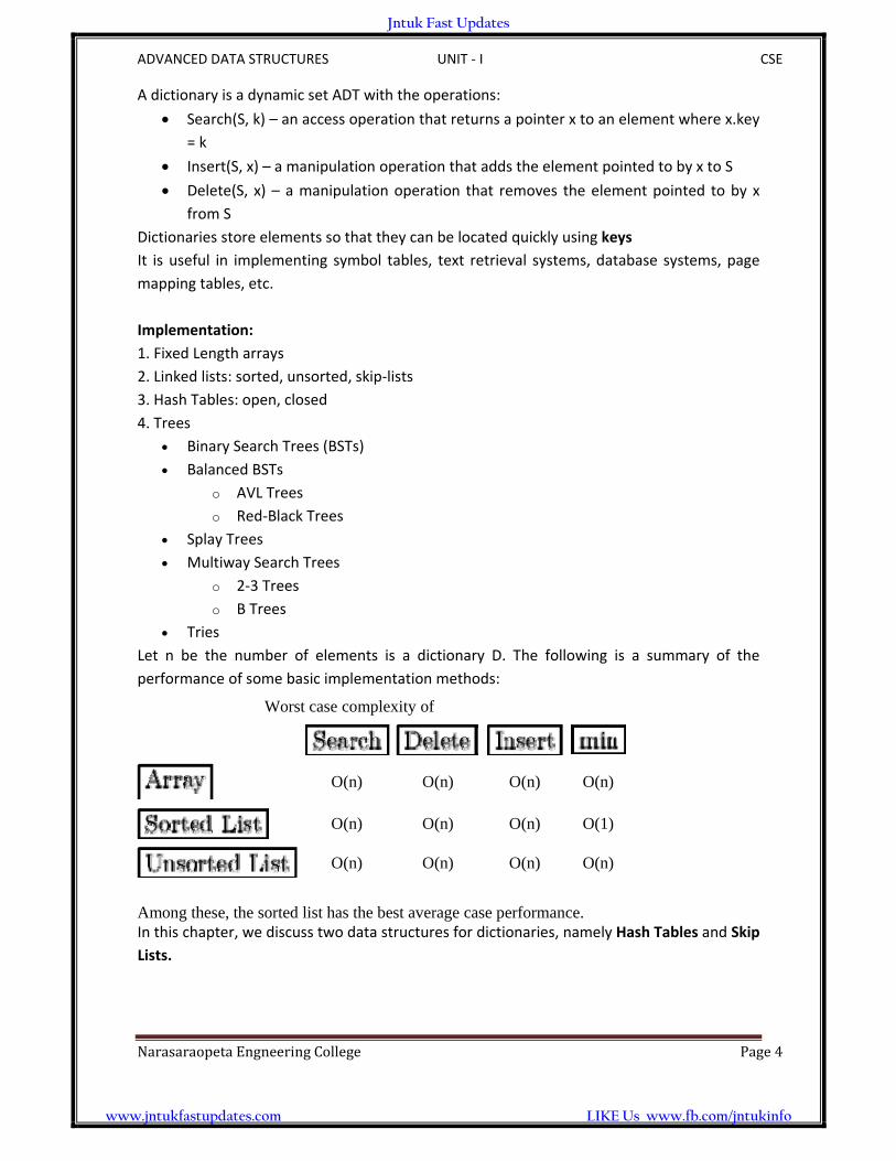
Let n be the number of elements is a dictionary D. The following is a summary of the
performance of some basic implementation methods:
Worst case complexity of
O(n) O(n) O(n) O(n)
O(n) O(n) O(n) O(1)
O(n) O(n) O(n) O(n)
Among these, the sorted list has the best average case performance. In this chapter, we discuss two data structures for dictionaries, namely Hash Tables and Skip
Lists.
Jntuk Fast Updates
www.jntukfastupdates.com LIKE Us www.fb.com/jntukinfo
ADVANCED DATA STRUCTURES UNIT ‐ I CSE
NarasaraopetaEngineeringCollege Page5
HASHING
Division Method:
One common method of determining a hash key of the division method of hashing
The formula that will be used is:
H(key) = key % no.of slots in the table
i.e. h(key) = key mod array size
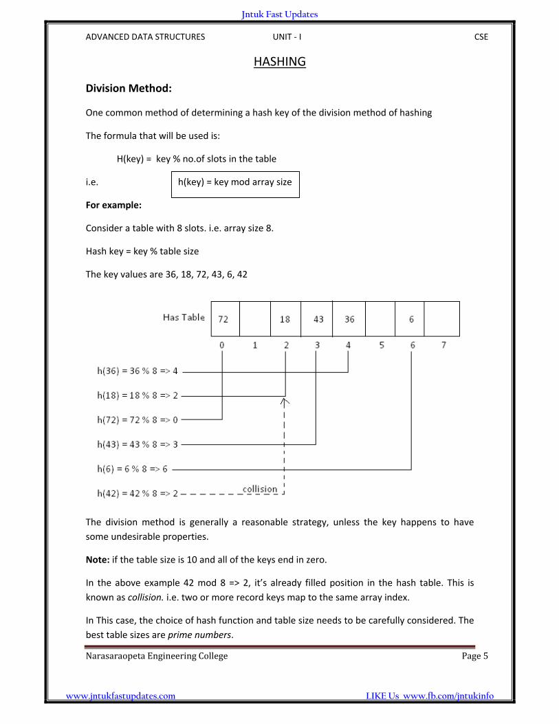
For example:
Consider a table with 8 slots. i.e. array size 8.
Hash key = key % table size
The key values are 36, 18, 72, 43, 6, 42
The division method is generally a reasonable strategy, unless the key happens to have
some undesirable properties.
Note: if the table size is 10 and all of the keys end in zero.
In the above example 42 mod 8 => 2, it’s already filled position in the hash table. This is
known as collision. i.e. two or more record keys map to the same array index.
In This case, the choice of hash function and table size needs to be carefully considered. The
best table sizes are prime numbers.
h(key) = key mod array size
Jntuk Fast Updates
www.jntukfastupdates.com LIKE Us www.fb.com/jntukinfo

ADVANCED DATA STRUCTURES UNIT ‐ I CSE
NarasaraopetaEngineeringCollege Page6
Multiplication method:
The simplest situation when the keys are floating –point numbers known to be in affixed
range.
For example:
If the keys are numbers that are greater than 0 and less than 1, we can just multiply by m
(table size) and round off to the nearest integer to get an address between 0 an m‐1.
Algorithm:
1. Choose constant A in the range 0 < A < 1. 2. Multiply key k by A. 3. Extract the fractional part of k*A 4. Multiply the fractional part by number of slots, m. 5. Take the floor of the result.
Mathematically
h( k ) = m ∙ (k∙A mod 1)
where k∙A mod 1 = k∙A − k∙A = fractional part of k∙A
Disadvantage: Slower than division method. Advantage: Value of m is not critical.
Example:
m = 8 (implies m = 23, p = 3)
w = 5
k = 21
Must have 0 < s < 25; choose s = 13 → A = 13/32.
h(k) = m ∙ (k∙A mod 1)
h( 21 ) = 8 ∙ (21∙13/32 mod 1) = 4
k∙A = 21 ∙ 13/32 = 273/32 = 8 17/32 → k∙A mod 1 = 17/32
→ m ∙ ( k∙A mod 1) = 8 ∙ 17/32 = 17/4 = 4 1/4 → m ∙ ( k∙A mod 1) = 4
So that h(21) = 4.
Jntuk Fast Updates
www.jntukfastupdates.com LIKE Us www.fb.com/jntukinfo

ADVANCED DATA STRUCTURES UNIT ‐ I CSE
NarasaraopetaEngineeringCollege Page7
Example: m = 8 (implies m = 23, p = 3) w = 5 k = 21 s = 13
k ∙ s = 21 ∙ 13
= 273
= 8 ∙ 25 + 17
= r1 . r0
r1 r0
= 8 ∙ 25 = 17 = 100012
Written in w = 5 bits, r0 = 100012 The p = 3 most significant bits of r0 is 1002 or 410, so h(21) = 4.
Exercise Example:
m = 4 (implies m = 22, p = 2) w = 3 k = 12 s = 5 0 < s < 2w = 23 = 8
k ∙ s = 12 ∙ 5
= ?
= ? ∙ 23 + ?
= r1 . r0
r1 r0
= ? ∙ 23 = ? = ?2
Written in w = 3 bits, r0 = ?2 The p = 2 most significant bits of r0 is ?2 or ?10, so h(12) = ?.
Jntuk Fast Updates
www.jntukfastupdates.com LIKE Us www.fb.com/jntukinfo

ADVANCED DATA STRUCTURES UNIT ‐ I CSE
NarasaraopetaEngineeringCollege Page8
Universal method:
Hashing is a fun idea that has lots of unexpected uses. Here, we look at a novel type of hash
function that makes it easy to create a family of universal hash functions. The method is
based on a random binary matrix and is very simple to implement.
The idea is very simple. Suppose you have an input data item that you have input data with
m – bits and you want a hash function that produces n – bits then first generate a random
binary matrix (M) of order nxm.
The hash function is h(x) = Mx Where x to be a binary vector
For example, Suppose you have a key 11, the binary form is 1011 and it is a four bit input
value(m) and want to generate output a three bit hash value(n).
Then generate a random matrix gives say:
( 0 1 0 0 ) M = ( 1 0 1 1 ) ( 1 1 0 1 ) and if the data value was 1011 the hash value would be computed as:
( 0 1 0 0 ) (1) (0) h(x) = Mx = ( 1 0 1 1 ) (0) = (1) ( 1 1 0 1 ) (1) (0) (1) There are a number of other ways to look at the way the arithmetic is done that suggest different ways of implementing the algorithm. The first is to notice that what you are doing is anding each row with the data column vector. That is taking the second row as an example: ( 1 0 1 1 )And (1 0 1 1) = (1 0 1 1) and then you add up the bits in the result: 1+0+1+1=1 now the index is 010, convert that into decimal is 2. There is no.of other ways to look at the way the arithmetic is done that suggest different ways of implementing the algorithm. Hashing gives an alternative approach that is often the fastest and most convenient way of solving these problems like AI – search programs, cryptography, networks, complexity theory.
Jntuk Fast Updates
www.jntukfastupdates.com LIKE Us www.fb.com/jntukinfo

ADVANCED DATA STRUCTURES UNIT ‐ I CSE
NarasaraopetaEngineeringCollege Page9
Collision Resolution Techniques: In general, a hashing function can map several keys into the same address. That leads to a collision. The colliding records must be stored and accessed as determined by a collision – resolution techniques. There are two broad classes of such techniques: Open Hashing (also called separate chaining) and Closed Hashing (also called open addressing) The difference between the two has to do with whether collision are stored outside the table (open hashing), or whether collision result in storing and of the records at another slot in the table (closed hashing). The particular hashing method that one uses depends on many factors. One important factor is the ratio of the no.of keys in the table to the no.of hash addresses. It is called load factor, and is given by: Load factor (α) = n/m, where n is no.of keys in the table and m is no.of hash address (table size)
Open Hashing: The simplest form of open hashing defines each slot in the hash table to be the head of a linked list. All records that hash to a particular slot are placed on that slot’s linked list. The below figure illustrates a hash table where each slot stores one record and a link pointer to the rest of the list. Consider the same example of division method:
Jntuk Fast Updates
www.jntukfastupdates.com LIKE Us www.fb.com/jntukinfo

ADVANCED DATA STRUCTURES UNIT ‐ I CSE
NarasaraopetaEngineeringCollege Page10
Any key that hash to the same index are simply added to the linked list; there is no need to search for empty cells in the array. This method is called separating chaining.
Closed Hashing (Open addressing): It resolves collisions in the prime area – that is that contains all of the home addresses. i.e. when a data item cannot be placed at the index calculated by the hash function, another location in the array is sought. There are different methods of open addressing, which vary in the method used to find the next vacant cell. They are (i) Linear probing (ii) Quadratic probing (iii) Pseudo random probing (iv) Double hashing (v) Key – offset Hashing with Linear probe: We resolve the collision by adding 1 to the current address. Assuming that the table is not full We apply division method of hashing Consider the example:
Add the keys 10, 5, and 15 to the above table H(k) = k mod table size 10 mod 8 = 2 a collision, so add 1 to the address then check is it empty or filled. If it is filled then apply the same function, like this we can place this key 10 in the index 5 cell.
If the physical end of the table is reached during the linear search will wrap around to the beginning of the table and continue from there. If an empty slot is not found before reaching the point of collision; the table is full
Jntuk Fast Updates
www.jntukfastupdates.com LIKE Us www.fb.com/jntukinfo

ADVANCED DATA STRUCTURES UNIT ‐ I CSE
NarasaraopetaEngineeringCollege Page11
A problem with the linear probe method is that it is possible for blocks of data to form when collisions are resolved. This is known as primary clustering. This means that any key that hashes into the cluster will require several attempts to resolve the collision. Linear probes have two advantages: First, They are quite simple to implement. Second, data tend to remain near their home address. Exercise Example: Insert the nodes 89, 18, 49, 58, and 69 into a hash table that holds 10 items using the division method. Hashing with Quadratic probe: In this probe, rather than always moving one spot, move ‘ i2 ‘ spots from the point of collision, where ‘i’ is the no. of attempts to resolve the collision. In linear probe, if the primary hash index is x, subsequent probe go to x+1, x+2, x+3 and so on. In Quadratic probing, probes go to x+1, x+4, x+9, and so on, the distance from the initial probe is the square of the step number: x+12, x+22, x+32, x+42 and so on. i.e., at first it picks the adjacent cell, if that is occupied, it tries 4 cells away, if that is occupied it tries 9 cells away, and so on. It eliminates the primary clustering problem with linear probe. Consider the above exercise problem, keys 89, 18, 49, 58, 69 with table size 10.
Here each key that hashes to same location will require a longer probe. This phenomenon is called secondary clustering. It is not a serious problem, but quadratic probing is not often used because there is a slightly better solution.
Jntuk Fast Updates
www.jntukfastupdates.com LIKE Us www.fb.com/jntukinfo
ADVANCED DATA STRUCTURES UNIT ‐ I CSE
NarasaraopetaEngineeringCollege Page12
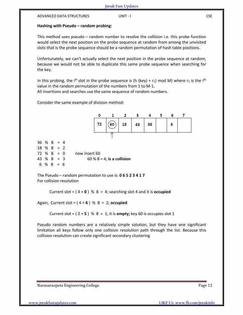
Hashing with Pseudo – random probing: This method uses pseudo – random number to resolve the collision i.e. this probe function would select the next position on the probe sequence at random from among the unvisited slots that is the probe sequence should be a random permutation of hash table positions. Unfortunately, we can’t actually select the next position in the probe sequence at random, because we would not be able to duplicate this same probe sequence when searching for the key. In this probing, the ith slot in the probe sequence is (h (key) + r1) mod M) where r1 is the ith value in the random permutation of the numbers from 1 to M‐1. All insertions and searches use the same sequence of random numbers. Consider the same example of division method:
36 % 8 = 4 18 % 8 = 2 72 % 8 = 0 now insert 60 43 % 8 = 3 60 % 8 = 4; is a collision 6 % 8 = 6 The Pseudo – random permutation to use is: 0 6 5 2 3 4 1 7 For collision resolution Current slot = ( 4 + 0 ) % 8 = 4; searching slot 4 and it is occupied Again, Current slot = ( 4 + 6 ) % 8 = 2; occupied Current slot = ( 2 + 5 ) % 8 = 1; it is empty; key 60 is occupies slot 1 Pseudo random numbers are a relatively simple solution, but they have one significant limitation all keys follow only one collision resolution path through the list. Because this collision resolution can create significant secondary clustering
Jntuk Fast Updates
www.jntukfastupdates.com LIKE Us www.fb.com/jntukinfo

ADVANCED DATA STRUCTURES UNIT ‐ I CSE
NarasaraopetaEngineeringCollege Page13
Double Hashing: Double hashing uses the idea of applying a second hash function to the key when a collision occurs. The result of the second hash function will be the number of positions from the point of collision to insert. There are a couple of requirements for the second function: It must never evaluate to 0 Must make sure that all cells can be probed
A popular second hash function is : H2(key) = R – (key % R) Where R is a prime number that is similar than the size of the table
Table size = 10 Hash1 (key) = key % 10 Hash2 (key) = 7 – (key % 7) Because 7 is a prime number than the size of the table Insert keys: 89, 18, 49, 58, 69 Hash (89) = 89 % 10 = 9 Hash (18) = 18 % 10 = 8 Hash1 (49) = 49 % 10 = 9; it’s a collision Hash2 (49) = 7 – (49 % 7) = 7; positions from location 9 Hash1 (58) = 58 % 10 =8; it’s a collision Hash2 (58) = 7 – (58 % 7) = 5; positions from location 8 NOTE: Linear probing ‘m’ distinct probe sequences, primary clustering Quadratic probing ‘m’ distinct probe sequences, no primary but secondary clustering Double hashing ‘m2’ distinct probe sequences, no primary and secondary clustering
Jntuk Fast Updates
www.jntukfastupdates.com LIKE Us www.fb.com/jntukinfo

ADVANCED DATA STRUCTURES UNIT ‐ I CSE
NarasaraopetaEngineeringCollege Page14
Key – offset: It is double hashing method that produces different collision paths for different keys. Where as the pseudo random – number generator produces a new address as a function of the previous address; key offset calculates the new address as a function of the old address and key. One of the simplest versions simply adds the quotient of key divided by the list size to the address to determine the next collision resolution address, as shown below
Offset = key / list size Address = ( ( offset + old address) modulo list size ) ) For example: The key is 166702 and list size is 307, using modulo ‐ division hashing method generates an address of 1. It’s a collision because there was a key 070918. Using key offset to calculate the next address, we get 237 as shown below
Offset = 166702 / 307 = 543 Address = ( ( 543 + 001) ) modulo 307 = 237 If 237 were also a collision, we would repeat the process to locate the next address, as shown below
Offset = 166702 / 307 = 543 Address = ( ( 543 + 237) ) modulo 307 = 166 If it is free, then place the key in this address.
Jntuk Fast Updates
www.jntukfastupdates.com LIKE Us www.fb.com/jntukinfo
ADVANCED DATA STRUCTURES UNIT ‐ I CSE
NarasaraopetaEngineeringCollege Page15
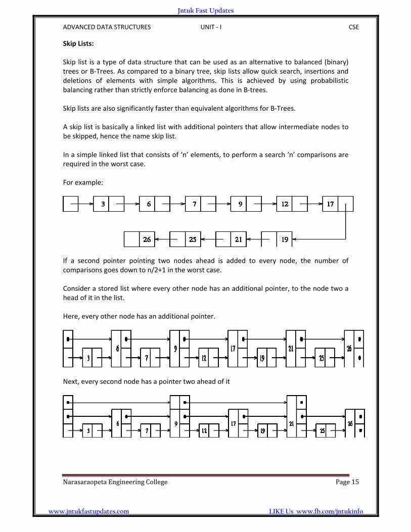
Skip Lists: Skip list is a type of data structure that can be used as an alternative to balanced (binary) trees or B‐Trees. As compared to a binary tree, skip lists allow quick search, insertions and deletions of elements with simple algorithms. This is achieved by using probabilistic balancing rather than strictly enforce balancing as done in B‐trees. Skip lists are also significantly faster than equivalent algorithms for B‐Trees. A skip list is basically a linked list with additional pointers that allow intermediate nodes to be skipped, hence the name skip list. In a simple linked list that consists of ‘n’ elements, to perform a search ‘n’ comparisons are required in the worst case. For example:
If a second pointer pointing two nodes ahead is added to every node, the number of comparisons goes down to n/2+1 in the worst case. Consider a stored list where every other node has an additional pointer, to the node two a head of it in the list. Here, every other node has an additional pointer.
Next, every second node has a pointer two ahead of it
Jntuk Fast Updates
www.jntukfastupdates.com LIKE Us www.fb.com/jntukinfo

ADVANCED DATA STRUCTURES UNIT ‐ I CSE
NarasaraopetaEngineeringCollege Page16
In the list of above figure, every second node has a pointer two ahead of it; every fourth
node has a pointer four ahead if it. Here we need to examine no more than + 2 nodes. In below figure, (every (2i)th node has a pointer (2i) node ahead (i = 1, 2,...); then the number
of nodes to be examined can be reduced to log2n while only doubling the number of pointers. Here, Every (2i)th node has a pointer to a node (2i)nodes ahead (i = 1, 2,...)
A node that has k forward pointers is called a level k node. If every (2i)th node has a pointer (2i) nodes ahead, then
# of level 1 nodes 50 % # of level 2 nodes 25 % # of level 3 nodes 12.5 %
Such a data structure can be used for fast searching but insertions and deletions will be extremely cumbersome, since levels of nodes will have to change.
What would happen if the levels of nodes were randomly chosen but in the same proportions (below figure)?
o level of a node is chosen randomly when the node is inserted o A node's ith pointer, instead of pointing to a node that is 2i ‐ 1 nodes ahead,
points to the next node of level i or higher. o In this case, insertions and deletions will not change the level of any node. o Some arrangements of levels would give poor execution times but it can be
shown that such arrangements are rare. Such a linked representation is called a skip list.
Each element is represented by a node the level of which is chosen randomly when the node is inserted, without regard for the number of elements in the data structure.
A level i node has i forward pointers, indexed 1 through i. There is no need to store the level of a node in the node.
Maxlevel is the maximum number of levels in a node. o Level of a list = Maxlevel o Level of empty list = 1 o Level of header = Maxlevel
Jntuk Fast Updates
www.jntukfastupdates.com LIKE Us www.fb.com/jntukinfo

ADVANCED DATA STRUCTURES UNIT ‐ I CSE
NarasaraopetaEngineeringCollege Page17
It is a skip list
Initialization: An element NIL is allocated and given a key greater than any legal key. All levels of all lists are terminated with NIL. A new list is initialized so that the level of list = maxlevel and all forward pointers of the list's header point to NIL Search: We search for an element by traversing forward pointers that do not overshoot the node containing the element being searched for. When no more progress can be made at the current level of forward pointers, the search moves down to the next level. When we can make no more progress at level 1, we must be immediately in front of the node that contains the desired element (if it is in the list). Insertion and Deletion:
Insertion and deletion are through search and splice update [i] contains a pointer to the rightmost node of level i or higher that is to the
left of the location of insertion or deletion. If an insertion generates a node with a level greater than the previous maximum
level, we update the maximum level and initialize appropriate portions of update list. After a deletion, we check to see if we have deleted the maximum level element of
the list and if so, decrease the maximum level of the list. Below figure provides an example of Insert and Delete. The pseudo ‐ code for Insert
and Delete is shown below.
Jntuk Fast Updates
www.jntukfastupdates.com LIKE Us www.fb.com/jntukinfo

ADVANCED DATA STRUCTURES UNIT ‐ I CSE
NarasaraopetaEngineeringCollege Page18
Analysis of Skip lists: In a skiplist of 16 elements, we may have
9 elements at level 1 3 elements at level 2 3 elements at level 3 1 element at level 6
One important question is: Where do we start our search? Analysis shows we should start from level L(n) where L(n) = log2n In general if p is the probability fraction,
L(n) = log n where p is the fraction of the nodes with level i pointers which also have level (i + 1) pointers.
However, starting at the highest level does not alter the efficiency in a significant way.
Another important question to ask is: What should be MaxLevel? A good choice is
MaxLevel = L(N) = log N where N is an upperbound on the number of elements is a skiplist.
Complexity of search, delete, insert is dominated by the time required to search for the appropriate element. This in turn is proportional to the length of the search path. This is determined by the pattern in which elements with different levels appear as we traverse the list.
Insert and delete involve additional cost proportional to the level of the node being inserted or deleted.
Jntuk Fast Updates
www.jntukfastupdates.com LIKE Us www.fb.com/jntukinfo

ADVANCED DATA STRUCTURES UNIT ‐ II CSE
NarasaraopetaEngineeringCollege Page19
BALANCED TREES
Introduction:
Tree:
A Tree consists of a finite set of elements, called nodes, and set of directed lines called
branches, that connect the nodes.
The no. of branches associated with a node is the degree of the node.
i.e. in ‐ degree and out ‐ degree.
A leaf is any node with an out degree of zero. i.e. no successor
A node that is not a root or leaf is known as an internal node
A node is a parent if it has successor node, conversely a node with a predecessor is
called child
A path is a sequence of nodes in which each node is adjacent to the next one
The level of a node is its distance from the root
The height of the tree is the level of the leaf in the longest path from the root plus 1
A sub tree is any connected structure below the root. Sub tree can also be further
divided into sub trees
Binary tree:
A binary tree is a tree in which no node can have more than two sub trees designated as the
left sub tree and the right sub tree.
Note: each sub tree is itself a binary tree.
Balance factor:
The balance factor of a binary tree is the difference in height between its left and right sub
trees. i.e. Balance factor = HL ‐ HR
In a balanced binary tree, the height of its sub trees differs by no more than one (its balance
factor is ‐1, 0, +1) and also its sub trees are also balanced.
Jntuk Fast Updates
www.jntukfastupdates.com LIKE Us www.fb.com/jntukinfo

ADVANCED DATA STRUCTURES UNIT ‐ II CSE
NarasaraopetaEngineeringCollege Page20
We now turn our attention to operations: search, insertion, deletion In the design of the linear list structure, we had two choices: an array or a linked list
The array structure provides a very efficient search algorithm, but its insertion and deletion algorithm are very inefficient.
The linked list structure provides efficient insertion and deletion, but its search algorithm is very inefficient.
What we need is a structure that provides an efficient search, at the same time efficient insertion and deletion algorithms. The binary search tree and the AVL tree provide that structure. Binary search tree: A binary search tree (BST) is a binary tree with the following properties:
All items in the left sub tree are less than the root.
All items in the right sub tree are greater than or equal to the root.
Each sub tree is itself a binary search tree. While the binary search tree is simple and easy to understand, it has one major problem: It is not balance. To over come this problem, AVL trees are designed, which are balanced.
AVL TREES In 1962, two Russian mathematicians, G.M Adelson – velskii and E.M Landis, aerated the balanced binary tree structure that is named after them – the AVL tree. An AVL tree is a search tree in which the heights of the sub trees differ by no more than 1. It is thus a balanced binary tree. An AVL tree is a binary tree that either is empty or consists of two AVL sub tree, TL and TR, whose heights differ by no more than 1.
| HL ‐ HR | < = 1 Where HL is the height of the left sub tree, HR is the height of the right sub tree The bar symbols indicate absolute value. NOTE: An AVL tree is a height balanced binary search tree.
Jntuk Fast Updates
www.jntukfastupdates.com LIKE Us www.fb.com/jntukinfo

ADVANCED DATA STRUCTURES UNIT ‐ II CSE
NarasaraopetaEngineeringCollege Page21
Consider an example: AVL tree
AVL Tree Balance factor: The Balance factor for any node in an AVL tree must be +1, 0, ‐1. We use the descriptive identifiers LH for left high (+1) to indicate that the length sub tree is higher than the right sub
tree EH for even high (0) to indicate that the sub tree are the same height RH for right high (‐1) to indicate that the left sub tree is shortest than the right sub
tree Balancing Trees: When ever we insert a node into a tree or delete a node from a tree, the resulting tree may be unbalanced then we must rebalance it. AVL trees are balanced by rotating nodes either to the left or to the right. Now, we are going to discuss the basic balancing algorithms. They are
1. Left of left: A sub tree of a tree that is left high has also become left high
2. Right of right: A sub tree of a tree that is right high has also become right high
3. Right of left: A sub tree of a tree that is left high has become right high
4. Left of right: A sub tree of a tree that is right high has become left high
Jntuk Fast Updates
www.jntukfastupdates.com LIKE Us www.fb.com/jntukinfo

ADVANCED DATA STRUCTURES UNIT ‐ II CSE
NarasaraopetaEngineeringCollege Page22
Left of left: When the out – of – balance condition has been created by a left high sub tree of a left high tree, we must balance the tree by rotating the out – of – balance node to the right. Let’s begin with a Simple case:
Complex case:
NOTE: In the above two cases, we have single rotation right.
Jntuk Fast Updates
www.jntukfastupdates.com LIKE Us www.fb.com/jntukinfo

ADVANCED DATA STRUCTURES UNIT ‐ II CSE
NarasaraopetaEngineeringCollege Page23
Right of Right: This case is the mirror of previous case. It contains a simple left rotation. Simple case: here, simple left rotation
Complex case: here, complex left rotation
NOTE: In the above two cases, we have single rotation left.
Jntuk Fast Updates
www.jntukfastupdates.com LIKE Us www.fb.com/jntukinfo

ADVANCED DATA STRUCTURES UNIT ‐ II CSE
NarasaraopetaEngineeringCollege Page24
Right of Left: The above two types required single rotation to balance the trees. Now we study about two out – of – balance conditions in which we need to rotate two nodes, one to the left and one to the right to balance the trees. Simple case: simple double rotation right.
Here, an out – of – balance tree in which the root is left high and left sub tree is right high – a right of left tree. To balance this tree, we first rotate the left sub tree to the left, then we rotate the root to the right, making the left node the new root. Complex case: complex double rotation right.
Jntuk Fast Updates
www.jntukfastupdates.com LIKE Us www.fb.com/jntukinfo

ADVANCED DATA STRUCTURES UNIT ‐ II CSE
NarasaraopetaEngineeringCollege Page25
Left of Right: This case is also complicated Simple case: simple double rotation
Complex case:
NOTE: In both cases, i.e. Right of left and Left of right, we have double rotations.
Jntuk Fast Updates
www.jntukfastupdates.com LIKE Us www.fb.com/jntukinfo

ADVANCED DATA STRUCTURES UNIT ‐ II CSE
NarasaraopetaEngineeringCollege Page26
Maximum Height of an AVL Tree: What is the maximum height of an AVL tree having exactly n nodes? To answer this question, we will pose the following question:
What is the minimum number of nodes (sparsest possible AVL tree) an AVL tree of height h can have ?
Let Fh be an AVL tree of height h, having the minimum number of nodes. Fh can be visualized as in Figure. Let Fl and Fr be AVL trees which are the left subtree and right subtree, respectively, of Fh. Then Fl or Fr must have height h-2. Suppose Fl has height h-1 so that Fr has height h-2. Note that Fr has to be an AVL tree having the minimum number of nodes among all AVL trees with height of h-1. Similarly, Fr will have the minimum number of nodes among all AVL trees of height h--2. Thus we have
| Fh| = | Fh - 1| + | Fh - 2| + 1 where | Fr| denotes the number of nodes in Fr. Such trees are called Fibonacci trees. See Figure. Some Fibonacci trees are shown in Figure 4.20. Note that | F0| = 1 and | F1| = 2. Adding 1 to both sides, we get
| Fh| + 1 = (| Fh - 1| + 1) + (| Fh - 2| + 1)
Thus the numbers | Fh| + 1 are Fibonacci numbers. Using the approximate formula for Fibonacci numbers, we get
| Fh| + 1
h 1.44log| Fn|
The sparsest possible AVL tree with n nodes has height
h 1.44log n
The worst case height of an AVL tree with n nodes is 1.44log n
Jntuk Fast Updates
www.jntukfastupdates.com LIKE Us www.fb.com/jntukinfo

ADVANCED DATA STRUCTURES UNIT ‐ II CSE
NarasaraopetaEngineeringCollege Page27
Figure 5.3: Fibonacci trees
Figure 5.4: Rotations in a binary search tree
Jntuk Fast Updates
www.jntukfastupdates.com LIKE Us www.fb.com/jntukinfo

ADVANCED DATA STRUCTURES UNIT ‐ II CSE
NarasaraopetaEngineeringCollege Page28
2 – 3 TREES
The basic idea behind maintaining a search tree is to make the insertion, deletion and searching operations efficient. In AVL Trees the searching operation is efficient. However, insertion & deletion involves rotation that makes the operation complicated. To eliminate this complication a data structure was designed, called as 2 ‐ 3 trees. To build a 2 – 3 tree there are certain rules that need to be followed. These rules are as follows: All the non – leaf nodes in a 2 – 3 tree must always have two or three non – empty
child nodes that are again 2 – 3 trees.
The level of all the leaf nodes must always be the same.
One single node can contain (left and right) then that node contains single data. The data occurring on left sub tree of that node is less than the data of the node and the data occurring on right sub tree of that node is greater than the data of the node.
If any node has three children (left, middle, right) then that node contains two data values, let say i and j where i < j, the data of all the nodes on the middle sub tree are greater than i but less than j and the data of all nodes on the right sub tree are greater than j.
Example of 2 – 3 Trees:
Jntuk Fast Updates
www.jntukfastupdates.com LIKE Us www.fb.com/jntukinfo

ADVANCED DATA STRUCTURES UNIT ‐ II CSE
NarasaraopetaEngineeringCollege Page29
Insertions in 2 – 3 Trees: Let us now try to understand the process of insertion of a value in 2 – 3 trees. To insert a value in a 2 – 3 trees we first need to search the position where the value can be inserted, and then the value and node in which the value is to be inserted are adjusted. Algorithm: Insert new leaf in appropriate place
Repeat until all non leaf nodes have 2 or 3 children If there is a node with 4 children, split the parent into two parent nodes, with 2
children each If you split the root, then add a new root
Adjust search values along insertion path
Example: Insert 5 Insert 21
Insert 8
Insert 63
5
Jntuk Fast Updates
www.jntukfastupdates.com LIKE Us www.fb.com/jntukinfo

ADVANCED DATA STRUCTURES UNIT ‐ II CSE
NarasaraopetaEngineeringCollege Page30
Insert 69
Insert 32
Insert 7, 9, 25
Jntuk Fast Updates
www.jntukfastupdates.com LIKE Us www.fb.com/jntukinfo

ADVANCED DATA STRUCTURES UNIT ‐ II CSE
NarasaraopetaEngineeringCollege Page31
Deletions in 2 – 3 Trees: Deletion of a value from a 2 – 3 trees is exactly opposite to insertion In case of insertion the node where the data is to be inserted is split if it already contains maximum no. of values. But in case of deletion, two nodes are merged if the node of the value to be deleted contains minimum number of values (i.e. only one value) Example 1: Consider a 2 – 3 trees
Delete 47
Delete 63
Jntuk Fast Updates
www.jntukfastupdates.com LIKE Us www.fb.com/jntukinfo
ADVANCED DATA STRUCTURES UNIT ‐ II CSE
NarasaraopetaEngineeringCollege Page32
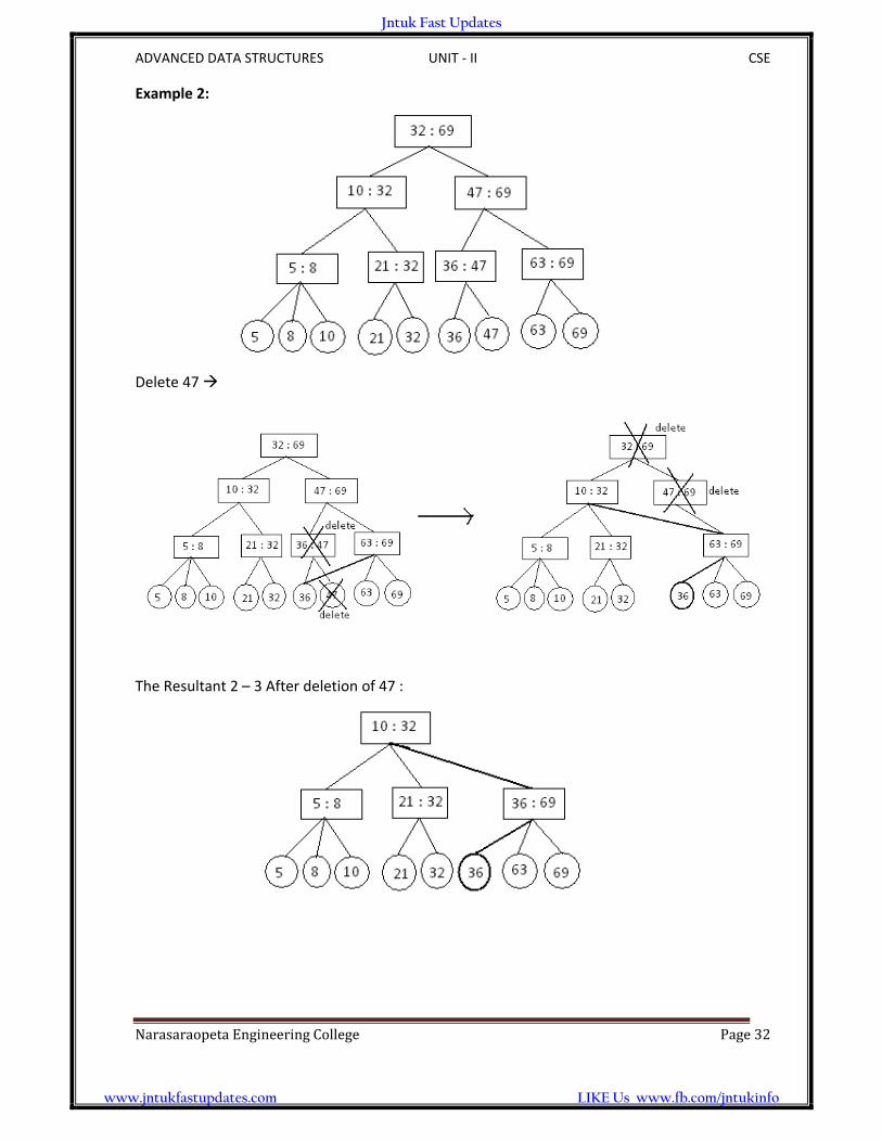
Example 2:
Delete 47
The Resultant 2 – 3 After deletion of 47 :
Jntuk Fast Updates
www.jntukfastupdates.com LIKE Us www.fb.com/jntukinfo

ADVANCED DATA STRUCTURES UNIT ‐ III CSE
NarasaraopetaEngineeringCollege Page33
PRIRORITY QUEUES
A priority queue is an important data type in computer science. Major operations supported
by priority queues are Inserting and Delete min.
Insert, which does the obvious thing; and Delete min, which finds, returns, and removes the
minimum element in the priority queue.
The priority queues are extensive use in.
Implementing schedulers in OS, and Distributed systems
Representing event lists in discrete event simulation
Implementing numerous graph algorithms efficiently
Selecting kth largest or kth smallest element in lists (order statistics problem)
Sorting Applications
Simple Implementation:
There are several ways to implement a priority queue
Linked list: stored and unsorted
Performing insertions at front in O(1) and traversing the list which requires O(N) time
To delete the minimum, we could insist that the list be kept always sorted: this
makes insertions expensive O(N) and delete‐mins cheap O(1)
Another way of implementing priority queues would be use a binary search tree.
This gives an O(log N) average running time for both operations
The basic data structure we will use will not require pointers and will support both
operations in O(log N) worst case time. The implementations we will use is known as
a binary – heap
Binary – Heaps:
Heaps (occasionally called as partially ordered trees) are a very popular data structure for
implementing priority queues.
Binary heaps are refer to merely as heaps, like binary search trees, heaps have two
properties, namely, a structure property and a heap order property.
Jntuk Fast Updates
www.jntukfastupdates.com LIKE Us www.fb.com/jntukinfo

ADVANCED DATA STRUCTURES UNIT ‐ III CSE
NarasaraopetaEngineeringCollege Page34
Structure property:
A heap is a binary tree that is completely filled, with the possible exception of the bottom
level, which is filled from left to right, such tree is known as a complete binary tree as shown
below
A binary heap is a complete binary tree with elements from a partially ordered set, such that
the element at every node is less than (or equal to) the element at its left child and the
element at its right child.
It is easy to show that a complete binary tree height ‘ h ‘ has between 2h and 2h+1‐1 nodes.
This implies that the height of a complete binary tree is log N , which is clearly O(log N).
One important observation is that because a complete binary tree is so regular, it can be
represented in an array and no pointers are necessary.
Since a heap is a complete binary tree, the elements can be conveniently stored in an array.
If an element is at position i in the array, then the left child will be in position 2i, the right
child will be in the position (2i+1), and the parent is in position i/2
The only problem with this implementation is that an estimate of the maximum heap size is
required in advance, but typically this is not a problem.
Because of the heap property, the minimum element will always be present at the root of
the heap. Thus the find min operation will have worst case O(1) running time.
Jntuk Fast Updates
www.jntukfastupdates.com LIKE Us www.fb.com/jntukinfo
ADVANCED DATA STRUCTURES UNIT ‐ III CSE
NarasaraopetaEngineeringCollege Page35
Heap – order property:
It is the property that allows operations to be performed quickly. Since we want to be able
to find the minimum quickly, it makes sense that the smallest element should be at the root.
If we consider that any sub tree should also be a heap, then any node should be smaller
than all of its descendants.
Applying this logic, we arrive at the heap order property. In a heap, for every node X, the
key in the parent of X is smaller than ( or equal to) the key X, with exception of the root.
(Which has no parent)?
NOTE: Binary heaps were first introduced by Williams in 1964.
NOTE: Binary Heap is either a min – heap or a max – heap. A min heap supports the insert
and delete min operations while a max heap supports the insert and delete max operations
Basic Heap Operations:
It is easy to perform the two required operations. All the work involves ensuring that the
heap order property is maintained.
Insert:
To insert an element say x, into the heap with n elements we first create a hole in position
(n+1) and see if the heap property is violated by putting x into the hole. If the heap property
is violated then we have found the current position for x. Otherwise we push ‐ up or
percolate – up x until the heap property is restored.
To do this we slide the element that is in the holes parent node into the hole thus bubbling
the hole up toward the root. We continue this process until x can be placed in the whole.
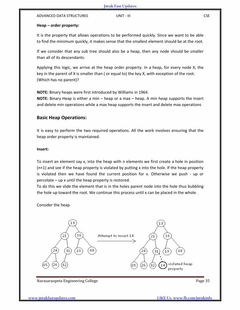
Consider the heap
Jntuk Fast Updates
www.jntukfastupdates.com LIKE Us www.fb.com/jntukinfo

ADVANCED DATA STRUCTURES UNIT ‐ III CSE
NarasaraopetaEngineeringCollege Page36
We create a hole in the next available heap location. Inserting 14 in the hole would violate
the heap order property so 31 is slid down into the hole. This strategy is continued until the
correct location for 14 is found.
This general strategy is known as a percolate up. i.e. the new element is percolated up the
heap until the correct location is found.
NOTE: Worst case complexity of insert is O(h) where h is the height of the heap. Thus
insertions are O(log n) where n is the no .of elements in the heap.
Delete min:
Where the minimum is deleted a hole is created at the root level. Since the heap now has
one less element and the heap is a complete binary tree, the element in the least position is
to be relocated.
This we first do by placing the last element in the hole created at the root. This will leave the
heap property possibly violated at the root level.
We now push – down or percolate – down the hole at the root until the violation of heap
property is stopped. While pushing down the hole it is important to slide it down to the less
of its two children (pushing up the latter). This is done so as not to create another violation
of heap property.
Consider the previous example:
First remove or delete min is 13.
Jntuk Fast Updates
www.jntukfastupdates.com LIKE Us www.fb.com/jntukinfo

ADVANCED DATA STRUCTURES UNIT ‐ III CSE
NarasaraopetaEngineeringCollege Page37
This general strategy is known as a percolate down. We use same technique as in the insert
routine to avoid the use of swaps in this routine.
NOTE: The worst case running time of delete min is O(log n) where n is the no. of elements
in the heap.
Jntuk Fast Updates
www.jntukfastupdates.com LIKE Us www.fb.com/jntukinfo

ADVANCED DATA STRUCTURES UNIT ‐ III CSE
NarasaraopetaEngineeringCollege Page38
Creating Heap:
The build heap operation takes as input n elements. The problem here is to create a heap of
these elements i.e. places them into an empty heap.
Obvious approach is to insert the n element one at a time into an initially empty
heap. Since each insert will take O(1) average and O(log n) worst case time, the total
running time of this algorithm would be O(n) average but O(n log n) worst case
Another approach proposed by Floyd in 1964 is to use a procedure called push –
down or percolate – down repeatedly. Starting with the array consisting of the given
n elements in the input – order.
If percolate – down (i) percolate down from node i, perform the algorithm to create
a heap – ordered tree.
for ( i = n/2 ; I > 0 ; i ‐‐)
percolate ‐ down (i)
Consider the tree is the unordered tree
Left: initial tree Right: after percolate – down (7)
Jntuk Fast Updates
www.jntukfastupdates.com LIKE Us www.fb.com/jntukinfo
ADVANCED DATA STRUCTURES UNIT ‐ III CSE
NarasaraopetaEngineeringCollege Page39
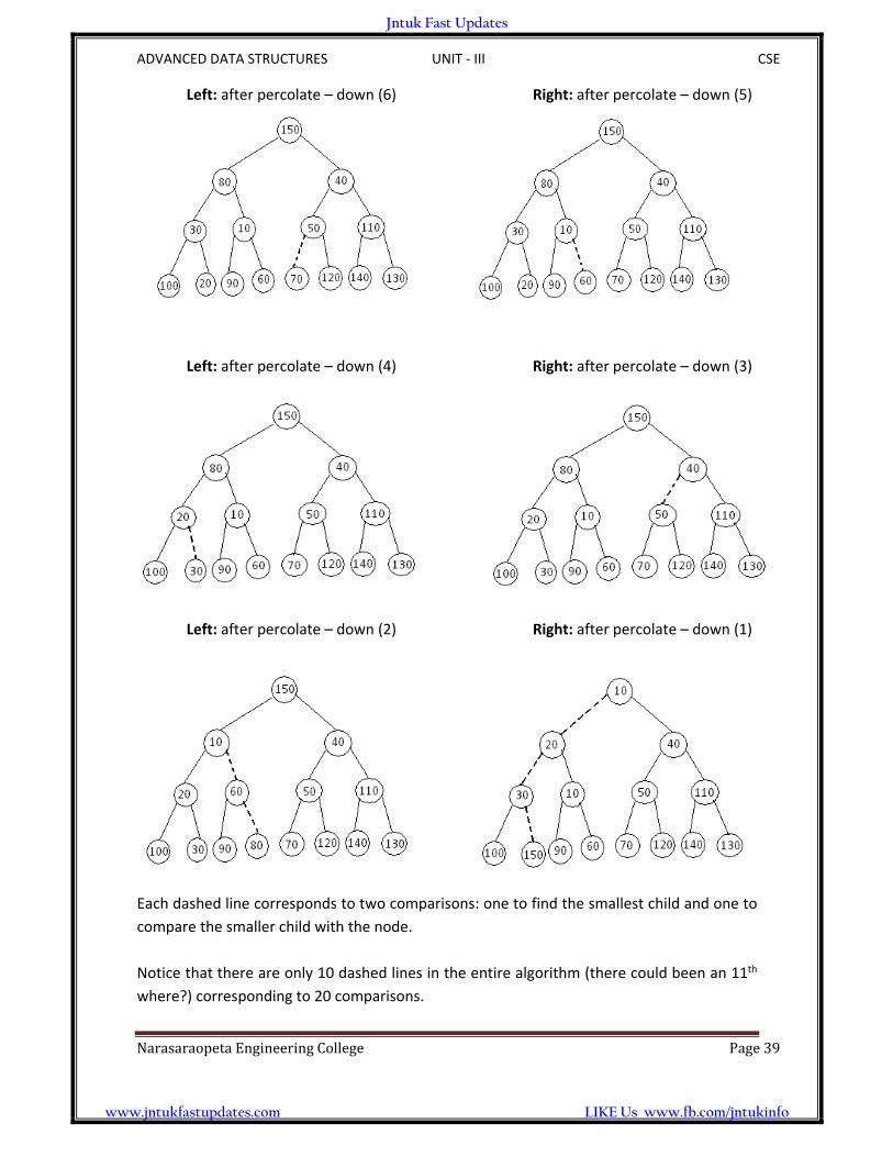
Left: after percolate – down (6) Right: after percolate – down (5)
Left: after percolate – down (4) Right: after percolate – down (3)
Left: after percolate – down (2) Right: after percolate – down (1)
Each dashed line corresponds to two comparisons: one to find the smallest child and one to
compare the smaller child with the node.
Notice that there are only 10 dashed lines in the entire algorithm (there could been an 11th
where?) corresponding to 20 comparisons.
Jntuk Fast Updates
www.jntukfastupdates.com LIKE Us www.fb.com/jntukinfo

ADVANCED DATA STRUCTURES UNIT ‐ III CSE
NarasaraopetaEngineeringCollege Page40
To bounding the running time of build heap, we must bound the no. of dashed lines. This
can be done by computing the sum of the heights of all the nodes in the heap, which is the
maximum no. of dashed lines. What we would like to show is that this is O(n).
THEOREM:
For the perfect binary tree of height h containing 2h+1‐1 nodes, the sum of the heights of
nodes is 2h+1‐1‐(h+1)
Proof:
It is easy to see that this tree consists of 1 node at height h, 2 nodes at height h‐1, 22 nodes
at height h‐2, and in general 2i nodes at height h‐i
The sum of the height of all the nodes is then S = ∑ 2i (h‐i) where i = o to h
S = h + 2 (h – 1) + 4 (h – 2) + 8 (h – 3) + 16 (h – 4) + ‐ ‐ ‐ + 2h – 1 (1)
Multiplying by 2 gives the equation
S = ‐ h + 2 + 4 + 8 + 16 + ‐ ‐ ‐ + 2h – 1 + 2h
There fore S = (2h+1 – 1) – (h+1) which proves the theorem
It is easy to see that the above is an upper bound on the sum of heights of nodes of a
complete binary tree. Since a complete binary tree of height h has between 2h and 2h+1
nodes, the above sum is there fore O(n)
Where n is the no. of nodes in the heap
Since the worst case complexity of the heap building algorithm is of the order of the sum of
height of the nodes of the heap built, we then have the worst case complexity of heap
building as O(n)
Jntuk Fast Updates
www.jntukfastupdates.com LIKE Us www.fb.com/jntukinfo

ADVANCED DATA STRUCTURES UNIT ‐ III CSE
NarasaraopetaEngineeringCollege Page41
Binomial Queues:
We know that previous concepts support merging, insertion, and delete min all effectively in
O(log n) time per operation but insertion take constant average time.
Binomial Queues support all three operations in O(log n) worst case time per operation, but
insertions take constant time on average.
Binomial Queue Structure:
It differs from all the priority queue implementations that a binomial queue is not a heap –
ordered tree but rather a collection of heap – ordered trees known as a forest.
Each of the heap – ordered trees is of a constrained from known as a binomial tree. There is
at most one binomial tree of every height.
A binomial tree of height 0 is a one – node tree
A binomial tree Bk of height k is formed by attaching a binomial tree Bk‐1 to the root
of another binomial tree Bk‐1
B0 B1 B2 B3
The above diagram shows binomial trees B0 B1 B2 and B3 from the diagram we see that a
binomial tree Bk consists of a root with children B0 B1 B2 ‐ ‐ ‐ Bk‐1
NOTE: Binomial tree of height k have exactly 2k nodes and the no. of nodes at depth d is the
binomial coefficient kCd
NOTE: If we impose heap order on the binomial tree and allow at most one binomial tree of
any height we can uniquely represent a priority queue of any size by a collection of binomial
trees (forest).
Jntuk Fast Updates
www.jntukfastupdates.com LIKE Us www.fb.com/jntukinfo

ADVANCED DATA STRUCTURES UNIT ‐ III CSE
NarasaraopetaEngineeringCollege Page42
For instance, a priority queue of size 13 could be represented by the forest B3 B2 B0
We might write this representation as 1 1 0 1. Which not only represent 13 in binary but
also represent the fact that B3 B2 and B0 are present in the representation and B1 is not.
As an example, a priority queue of six elements could be represented as in below figure
H1:
Figure: Binomial queue H1 with six elements
Binomial Queue operations:
Find – min:
This is implemented by scanning the roots of the entire tree. Since there are at most log n
different trees, the minimum can be found in O(log n) time.
Alternatively, one can keep track of the current minimum and perform find – min in O(1)
time. If we remember to update the minimum if it changes during other operations.
Merge:
Merging two binomial queues is a conceptually easy operation, which we will describe by
example.
Consider the two binomial queues H1 and H2 with six and seven elements respectively as
shown below.
H1: with 6 elements
Jntuk Fast Updates
www.jntukfastupdates.com LIKE Us www.fb.com/jntukinfo

ADVANCED DATA STRUCTURES UNIT ‐ III CSE
NarasaraopetaEngineeringCollege Page43
H2: with 7 elements
Merge of two B1 trees (i.e. 21 = 2 nodes) in H1 and H2. i.e.
Now we left with 1 tree of height 0 and 3 trees of height 2
Binomial queue H3: the result of merging H1 and H2
H3: with 13 elements
Jntuk Fast Updates
www.jntukfastupdates.com LIKE Us www.fb.com/jntukinfo

ADVANCED DATA STRUCTURES UNIT ‐ III CSE
NarasaraopetaEngineeringCollege Page44
The merging is performed by essentially adding the two queues together.
Let H3 be the new binomial queue.
Since H1 has no binomial tree of height 0, and H2 does, we can just use the binomial tree of
height o in H2 as part of H3.
Next, we add binomial trees of height 1.
Since both H1 and H2 have binomial tree of height 1, we merge them by making the larger
root a sub tree of the smaller, creating a binomial tree of height 2.
Thus, H3 will not have a binomial tree of height 1 as shown in the above diagrams.
There are now three binomial trees of height 2, namely, the original trees in both H1 and H2
plus the tree formed by adding of height 1 tree in both H1 and H2.
We keep one binomial tree of height 2 in H3 and merge the other two, creating a binomial
tree of height 3.
Since H1 and H2 have no trees of height 3, this tree becomes part of H3 and we are finished.
The resulting binomial queue is as shown in above figure.
Since merging two binomial trees takes constant time with almost any reasonable
implementation, and there are O(log n) binomial tree, the merge takes O(log n) time in the
worst case.
To make this operation efficient, we need to keep the trees in the binomial queue sorted by
height, which is certainly a simple thing to do.
Insertion:
Insertion is a special case of merging, since we merely create a one – node tree and
perform a merge.
The worst – case time of this operation is likewise O(log n)
More precisely, if the priority queue into which the element is being inserted has the
property that the smallest non existent binomial tree is Bi the running time is
proportional to i+1.
Jntuk Fast Updates
www.jntukfastupdates.com LIKE Us www.fb.com/jntukinfo

ADVANCED DATA STRUCTURES UNIT ‐ III CSE
NarasaraopetaEngineeringCollege Page45
For example:
In The previous example, H3 is missing a binomial tree of height 1, so the insertion will
terminate in two steps. Since each tree in a binomial queue is present with probability ½.
If we define the random variable X as representing the no. of steps in an insert operation,
then
X = 1 with probability 1/2 (B0 not present)
X = 2 with probability 1/2 (B0 and B1 not present)
X = 3 with probability 1/8
Thus average number of steps in an insert operation = 2.
Thus we expect an insertion to terminate in two steps on the average. Further more
performing n inserts on an initially empty binomial queue will take O(n) worst case time.
In deed it is possible to do this operation using only (n ‐ 1) comparisons.
Consider an example, the binomial queue that are formed by inserting 1 through 7 in order.
After 1 is inserted:
After 2 is inserted:
After 3 is inserted:
After 4 is inserted:
Jntuk Fast Updates
www.jntukfastupdates.com LIKE Us www.fb.com/jntukinfo

ADVANCED DATA STRUCTURES UNIT ‐ III CSE
NarasaraopetaEngineeringCollege Page46
After 5 is inserted:
After 6 is inserted:
After 7 is inserted:
If we insert 8 then
Inserting 4 shows off a bad case, we merge 4 with B0 obtaining a new tree of height 1. We
merge this tree with B1 obtaining a tree of height 2 which is the new priority queue.
The next insertion after 7 is another bad case and would require three merges.
Jntuk Fast Updates
www.jntukfastupdates.com LIKE Us www.fb.com/jntukinfo

ADVANCED DATA STRUCTURES UNIT ‐ III CSE
NarasaraopetaEngineeringCollege Page47
Delete min:
A delete min can be performed by first finding the binomial tree with the smallest
root.
Let this tree be Bk and let the original priority queue be H
Remove the binomial tree Bk from the forest of trees in H forming the new binomial
queue H′
Now remove the root of Bk creating binomial trees B0 B1 ‐ ‐ ‐ Bk – 1 which collectively
from priority queue H″.
Finish the operation by merging H′ & H″
Consider the same example of merge operation which has H3.
H3:
The minimum root is 12 so we obtain the two priority queues H′ & H″
The binomial queue that results from merging H′ & H″ is as shown below
NOTE: The entire delete min operation takes O(log n) worst case time
Jntuk Fast Updates
www.jntukfastupdates.com LIKE Us www.fb.com/jntukinfo

ADVANCED DATA STRUCTURES UNIT ‐ III CSE
NarasaraopetaEngineeringCollege Page48
Binomial Amortized Analysis:
Amortized Analysis of Merge
To merge two binomial queues, an operation similar to addition of binary integers is
performed:
At any stage, we may have zero, one, two, or three Bk trees, depending on whether or not
the two priority queues contain a Bk tree and whether or not a Bk tree is carried over from
the previous step.
If there is zero or more Bk tree, it is placed as a tree in the resulting binomial queue.
If there are two, they are merged into a Bk + 1 tree and carried over
If there are three, one is retained and other two merged.
Result 1:
A binomial queue of n elements can be built by n successive insertions in 0(n) time. Brute force Analysis
Define the cost of each insertions to be o 1time unit + an extra unit for each linking step
thus the total will be n units plus the total number of linking steps. o The 1st, 3rd, ... and each odd-numbered step requires no linking steps since
there is no B0 present. o A quarter of the insertions require only one linking step: 2nd, 6th, 10, ... o One eighth of insertions require two linking steps.
We could do all this and bound the number of linking steps by n.
The above analysis will not help when we try to analyze a sequence of operations that include more than just insertions.
Amortized Analysis
Consider the result of an insertion.
o If there is no B0 tree, then the insertion costs one time unit. The result of insertion is that there is now a B0 tree and the forest has one more tree.
o If there is a B0 tree but not B1 tree, then insertion costs 2 time units. The new forest will have a B1 tree but not a B0 tree. Thus number of trees in the forest is unchanged.
o An insertion that costs 3 time units will create a B2 tree but destroy a B0 and B1, yielding one less tree in the forest.
o In general, an insertion that costs c units results in a net increase of 2 - c trees. Since
a Bc - 1 tree is created
all Bi trees, 0 i c - 1 are removed.
Jntuk Fast Updates
www.jntukfastupdates.com LIKE Us www.fb.com/jntukinfo

ADVANCED DATA STRUCTURES UNIT ‐ III CSE
NarasaraopetaEngineeringCollege Page49
Thus expensive insertions remove trees and cheap insertions create trees.
Let ti =
ci =
We have
c0 = 0
ti + (ci - ci - 1) = 2
Result 2:
The amortized running times of Insert, Delete‐min, and Merge are 0(1), 0(log n), and
0(log n) respectively.
Potential function = # of trees in the queue
To prove this result we choose:
Insertion
ti =
ci =
ai = ti + (ci ‐ ci ‐ 1)
ai = 2 i
= 2n ‐ (cn ‐ c0)
As long as (cn ‐ c0) is positive, we are done.
In any case (cn ‐ c0) is bounded by log n if we start with an empty tree.
Merge:
Assume that the two queues to be merged have n1 and n2nodes with T1 and T2 trees. Let n =
n1+ n2. Actual time to perform merge is given by:
ti = 0(logn1 + logn2)
= 0(max(logn1, logn2)
= 0(log n)
(ci ‐ ci ‐ 1) is at most (log n) since there can be at most (log n) trees after merge.
Deletemin:
The analysis here follows the same argument as for merge.
Jntuk Fast Updates
www.jntukfastupdates.com LIKE Us www.fb.com/jntukinfo
ADVANCED DATA STRUCTURES UNIT ‐ III CSE
NarasaraopetaEngineeringCollege Page50
Lazy Binomial Queues:
Binomial queues in which merging is done lazily.
Here, to merge two binomial queues, we simply concatenate the two lists of binomial trees.
In the resulting forest, there may be several trees of the same size.
Because of the lazy merge, merge and insert are both worst case 0(1) time.
Delete min:
o Convert lazy binomial queue into a standard binomial queue
o Do delete min as in standard queue.
Fibonacci Heaps
Fibonacci heap supports all basic heap operations in 0(1) amortized time, with the exception
of delete min and delete which take 0(log n) amortized time.
Fibonacci heaps generalize binomial queues by adding two new concepts:
A different implementation of decrease‐key
Lazy merging: Two heaps are merged only when it is required.
It can be shown in a Fibonacci heap that any node of rank r 1 has at least Fr + 1
descendant.
Jntuk Fast Updates
www.jntukfastupdates.com LIKE Us www.fb.com/jntukinfo
ADVANCED DATA STRUCTURES UNIT ‐ IV CSE
NarasaraopetaEngineeringCollege Page51
GRAPHS
In this chapter, we turn our attention to a data structure – Graphs ‐ that differs from all of
the other in one major concept: each node may have multiple predecessors as well as
multiple successors.
Graphs are very useful structures. They can be used to solve complex routing problems,
such as designing and routing airlines among the airports they serve. Similarly, they can be
used to route messages over a computer network from one node to another.
Basic Concepts:
A graph is a collection of nodes, called vertices and a collection of segments called lines
connecting pair of vertices. In other words a graph consists of two sets, a set of vertices and
set of lines.
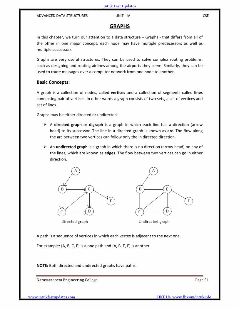
Graphs may be either directed or undirected.
A directed graph or digraph is a graph in which each line has a direction (arrow
head) to its successor. The line in a directed graph is known as arc. The flow along
the arc between two vertices can follow only the in directed direction.
An undirected graph is a graph in which there is no direction (arrow head) on any of
the lines, which are known as edges. The flow between two vertices can go in either
direction.
A path is a sequence of vertices in which each vertex is adjacent to the next one.
For example: {A, B, C, E} is a one path and {A, B, E, F} is another.
NOTE: Both directed and undirected graphs have paths.
Jntuk Fast Updates
www.jntukfastupdates.com LIKE Us www.fb.com/jntukinfo

ADVANCED DATA STRUCTURES UNIT ‐ IV CSE
NarasaraopetaEngineeringCollege Page52
Two vertices in a graph are said to be adjacent vertices (or neighbors) if there is a path of
length 1 connecting them.
Consider the above diagrams
In directed graph, B is adjacent to A, where as E is not adjacent to D; but D is adjacent to E.
In undirected graph, E and D are adjacent, but D and F are not.
A cycle is a path, it start with vertex and ends with same vertex.
Example:
A‐B‐C‐A is a cycle
A loop is a special case of cycle in which a single arc begins and ends with the same vertex.
In a loop the end points of the line are the same.
Two vertices are said to be connected if there is a path between them. A graph is said to be
connected if, ignoring direction, there is a path from any vertex to any other vertex.
A directed graph is strongly connected if there is a path from each vertex to every other
vertex in the digraph.
A directed graph is weakly connected if at least two vertices are connected (A connected
undirected graph would always be strongly connected, so the concept is not normally used
with undirected graphs)
Jntuk Fast Updates
www.jntukfastupdates.com LIKE Us www.fb.com/jntukinfo

ADVANCED DATA STRUCTURES UNIT ‐ IV CSE
NarasaraopetaEngineeringCollege Page53
A graph is a disjoint graph if it is not connected
The degree of a vertex is the no/of lines incident to it
The out ‐ degree of a vertex in a digraph is the no. of arcs leaving the vertex
The in ‐ degree is the no. of arcs entering the vertex
For example: for vertex B; degree = 3, in ‐ degree = 1, out ‐ degree = 2
NOTE: A tree is a graph in which each vertex has only one predecessor; how ever a graph is
not a tree.
Operations on Graphs:
There are six primitive graph operations that provide the basic modules needed to maintain
a graph. They are
1. Insert a vertex
2. Delete a vertex
3. Add an edge
4. Delete an edge
5. Find a vertex
6. Traverse a graph
Vertex insertion:
Insert vertex adds a new vertex to a graph
When a vertex is inserted it is disjoint; it is not connected to any other vertices in the list
After inserting a vertex it must be connected
The below diagram shows a graph before and after a new vertex is added
Jntuk Fast Updates
www.jntukfastupdates.com LIKE Us www.fb.com/jntukinfo

ADVANCED DATA STRUCTURES UNIT ‐ IV CSE
NarasaraopetaEngineeringCollege Page54
Algorithm:
Algorithm insert vertex (graph, data)
Allocate memory for new vertex
Store data in new vertex
Increment graph count
if (empty graph)
Set graph first to new node
else
Search for insertion point
if (inserting before first vertex)
Set graph first to new vertex
else
Insert new vertex in sequence
end if
end insert vertex
Vertex deletion:
Delete vertex removes a vertex from the graph when a vertex is deleted; all connecting
edges are also removed
Jntuk Fast Updates
www.jntukfastupdates.com LIKE Us www.fb.com/jntukinfo

ADVANCED DATA STRUCTURES UNIT ‐ IV CSE
NarasaraopetaEngineeringCollege Page55
Algorithm:
Algorithm delete vertex(graph, key)
Return +1 if successful
‐1 if degree not zero
‐2 if key is not found
if (empty graph)
return ‐2;
end if
search for vertex to be deleted
if (not found)
return ‐2;
end if
if ( vertex indegree > 0 or indegree > 0)
return ‐1;
end if
delete vertex
decrement graph count
return 1;
end delete vertex
Edge addition:
Add edge connects a vertex to destination vertex. If a vertex requires multiple edges, add
an edge must be called once for each adjacent vertex. To add an edge, two vertices must be
specified. If the graph is a digraph, one of the vertices must be specified as the source and
one as the destination.
The below diagram shows adding an edge {A, E} to the graph
Jntuk Fast Updates
www.jntukfastupdates.com LIKE Us www.fb.com/jntukinfo

ADVANCED DATA STRUCTURES UNIT ‐ IV CSE
NarasaraopetaEngineeringCollege Page56
Algorithm:
Algorithm insertArc (graph, fromkey, tokey)
Return +1 if successful
‐2 if fromkey not found
‐3 if tokey not found
Allocate memory for new arc
Search and set fromvertex
if (fromvertex not found)
return ‐2;
end if
search and set tovertex
if (tovertex not found)
return ‐3;
end if
increment fromvertex outdegree
increment tovertex indegree
set arc destination to tovertex
if ( fromvertex arc list empty)
set fromvertex firstArc to new arc
set new arc nextArc to null
return 1;
end if
find insertion point in arc list
if (insert at beginning of arc list)
set fromvertex firstArc to new arc
else
insert in arc list
end if
return 1;
end insertArc
Jntuk Fast Updates
www.jntukfastupdates.com LIKE Us www.fb.com/jntukinfo

ADVANCED DATA STRUCTURES UNIT ‐ IV CSE
NarasaraopetaEngineeringCollege Page57
Edge deletion:
Delete edge removes one edge from a graph.
Below diagram shows that deleted the edge {B, E} from the graph
Algorithm:
Algorithm deleteArc(graph, fromkey, tokey)
Return +1 if successful
‐2 if fromkey not found
‐3 if tokey not found
if (empty graph)
return ‐2;
end if
search and set fromvertex to tovertex with key equal to fromkey
if (fromvertex arc not found)
return ‐2;
end if
if (fromvertex arc list null)
return ‐3;
end if
search and find arc with key equal to tokey
if (tokey not found)
return ‐3;
enf if
set tovertex to arc destination
delete arc
decrement fromvertex outdegree
decrement tovertex indegree
return 1;
end deleteArc
Jntuk Fast Updates
www.jntukfastupdates.com LIKE Us www.fb.com/jntukinfo

ADVANCED DATA STRUCTURES UNIT ‐ IV CSE
NarasaraopetaEngineeringCollege Page58
Find vertex:
Find vertex traverse a graph, looking for a specified vertex. If the vertex is found its data are
returned and if it is not found then an error is indicated.
The below figure shows find vertex traverses the graph, looking for vertex C
Algorithm:
Algorithm retrievevertex (graph, key, dataout)
Return +1 if successful
‐2 if key not found
if (empty graph)
return ‐2;
end if
search for vertex
if (vertex found)
move locptr data to dataout
return 1;
else
return ‐2;
end if
end retrievevertex
Jntuk Fast Updates
www.jntukfastupdates.com LIKE Us www.fb.com/jntukinfo

ADVANCED DATA STRUCTURES UNIT ‐ IV CSE
NarasaraopetaEngineeringCollege Page59
Graph Storage Structure:
To represent a graph, we need to store two sets. The first set represents the vertices of the
graph and the second set represents the edges or arcs. The two most common structures
used to store these sets are arrays and linked lists. Although the arrays offer some simplicity
this is a major limitation.
Adjacency Matrix:
The adjacency matrix uses a vector (one – dimensional array) for the vertices and a matrix
(two – dimensional array) to store the edges. If two vertices are adjacent – that is if there is
no edge between them, intersect is set to 0.
If the graph is directed, the intersection in the adjacency matrix indicates the direction
In the below diagram, there is an arc from sources vertex B to destination vertex C. In the
adjacency matrix, this arc is seen as a 1 in the intersection from B (on the left) to C (on the
top). Because there is no arc from C to B, however, the intersection from C to B is 0.
Jntuk Fast Updates
www.jntukfastupdates.com LIKE Us www.fb.com/jntukinfo
ADVANCED DATA STRUCTURES UNIT ‐ IV CSE
NarasaraopetaEngineeringCollege Page60
NOTE: In adjacency matrix representation, we use a vector to store the vertices and a matrix
to store the edges.
In addition to the limitation that the size of graph must be know before the program starts,
there is another serious limitation in the adjacency matrix: only one edge can be stored
between any two vertices. Although this limitation does not prevent many graphs from
using the matrix format, some network structures require multiple lines between vertices.
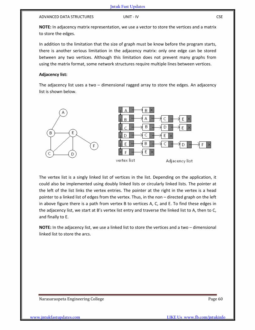
Adjacency list:
The adjacency list uses a two – dimensional ragged array to store the edges. An adjacency
list is shown below.
The vertex list is a singly linked list of vertices in the list. Depending on the application, it
could also be implemented using doubly linked lists or circularly linked lists. The pointer at
the left of the list links the vertex entries. The pointer at the right in the vertex is a head
pointer to a linked list of edges from the vertex. Thus, in the non – directed graph on the left
in above figure there is a path from vertex B to vertices A, C, and E. To find these edges in
the adjacency list, we start at B’s vertex list entry and traverse the linked list to A, then to C,
and finally to E.
NOTE: In the adjacency list, we use a linked list to store the vertices and a two – dimensional
linked list to store the arcs.
Jntuk Fast Updates
www.jntukfastupdates.com LIKE Us www.fb.com/jntukinfo
ADVANCED DATA STRUCTURES UNIT ‐ IV CSE
NarasaraopetaEngineeringCollege Page61
Traverse graph:
There is always at least one application that requires that all vertices in a given graph be
visited; as we traverse the graph, we set the visited flag to on to indicate that the data have
been processed
That is traversal of a graph means visiting each of its nodes exactly once. This is
accomplished by visiting the nodes in a systematic manner
There are two standard graph traversals: depth first and breadth first. Both use visited flag
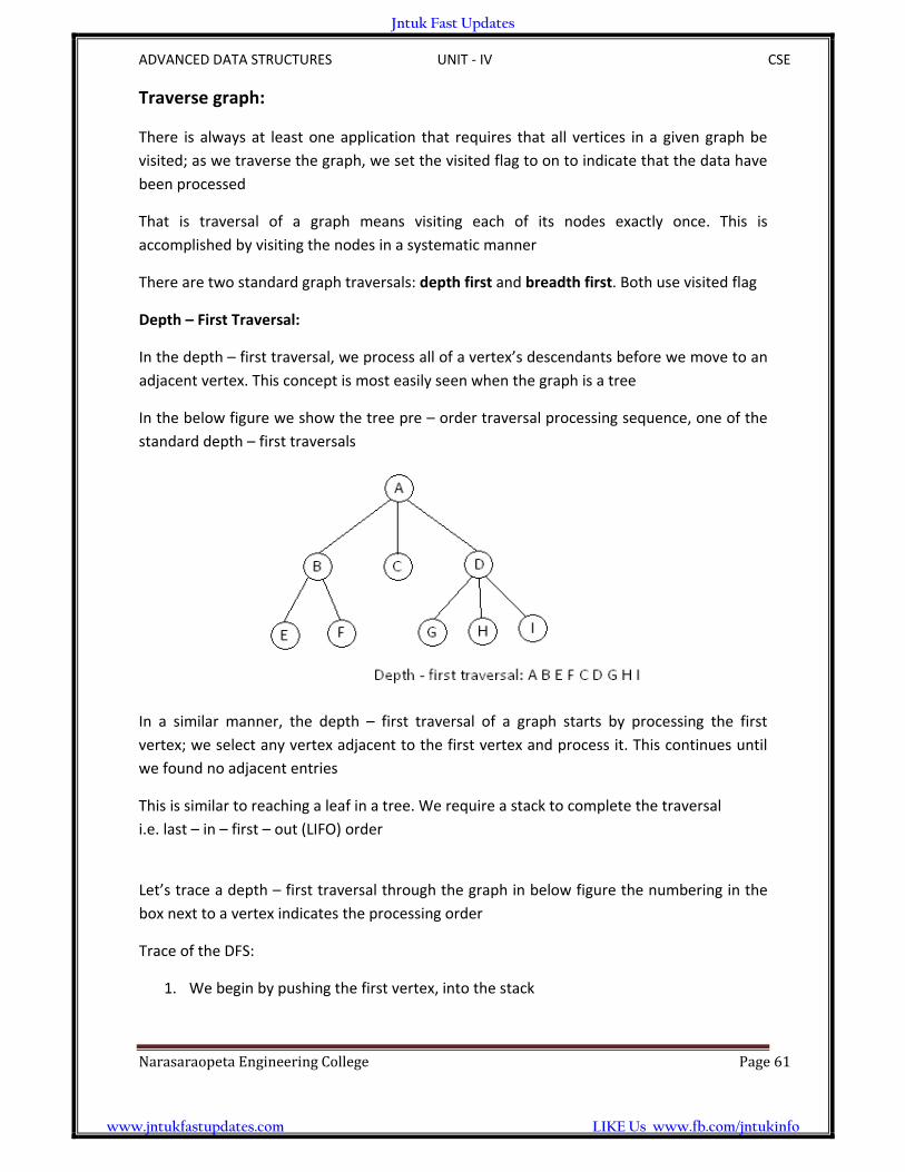
Depth – First Traversal:
In the depth – first traversal, we process all of a vertex’s descendants before we move to an
adjacent vertex. This concept is most easily seen when the graph is a tree
In the below figure we show the tree pre – order traversal processing sequence, one of the
standard depth – first traversals
In a similar manner, the depth – first traversal of a graph starts by processing the first
vertex; we select any vertex adjacent to the first vertex and process it. This continues until
we found no adjacent entries
This is similar to reaching a leaf in a tree. We require a stack to complete the traversal
i.e. last – in – first – out (LIFO) order
Let’s trace a depth – first traversal through the graph in below figure the numbering in the
box next to a vertex indicates the processing order
Trace of the DFS:
1. We begin by pushing the first vertex, into the stack
Jntuk Fast Updates
www.jntukfastupdates.com LIKE Us www.fb.com/jntukinfo

ADVANCED DATA STRUCTURES UNIT ‐ IV CSE
NarasaraopetaEngineeringCollege Page62
2. We then loop, pop the stack and after processing the vertex, push all of the adjacent
vertices into the stack
3. When the stack is empty traversal is completed
NOTE: In the depth – first traversal, all of a node’s descendents are processed before
moving to an adjacent node
Consider the above graph, let node A be the starting vertex
1. Begin with node A push onto stack
2. While stack not equal to empty
Pop A; state A is visited
Push nodes adjacent to A to stack and make their state waiting
3. Pop X; state B is visited
Push nodes adjacent to X into stack
4. Pop H; state H is visited
Push nodes adjacent to H into stack already G is in waiting state, then push nodes E
and P
5. Pop P; state P is visited
Jntuk Fast Updates
www.jntukfastupdates.com LIKE Us www.fb.com/jntukinfo

ADVANCED DATA STRUCTURES UNIT ‐ IV CSE
NarasaraopetaEngineeringCollege Page63
Push nodes adjacent to P are H, G, E; H is already in visited state, G and E are in
waiting state
6. Pop E; state E is visited
Push adjacent nodes, H is already visited, so push Y and M into the stack
7. Pop Y; state Y is visited
Push nodes adjacent to Y into stack, E is visited, M already in waiting state
8. Pop M; state M is visited
Push nodes adjacent to M, which is J
9. Pop J; state J is visited
No nodes are there to be process
10. Pop G; state G is visited
Now the stack is empty
The depth – first order of the visited nodes are A X H P E Y M J G
Breadth – First traversal:
In the breadth – first traversal of a graph, we process all adjacent vertices of a vertex before
going to the next level. We first saw the breadth – first traversal of a tree as shown in below
This traversal starts at level 0 and then processes all the vertices in level 1 before going on
to process the vertices in level 2.
The breadth – first traversal of a graph follows the same concept, begin by picking a starting
vertex A after processing it, process all of its adjacent vertices and continue this process
until get no adjacent vertices
Jntuk Fast Updates
www.jntukfastupdates.com LIKE Us www.fb.com/jntukinfo
ADVANCED DATA STRUCTURES UNIT ‐ IV CSE
NarasaraopetaEngineeringCollege Page64
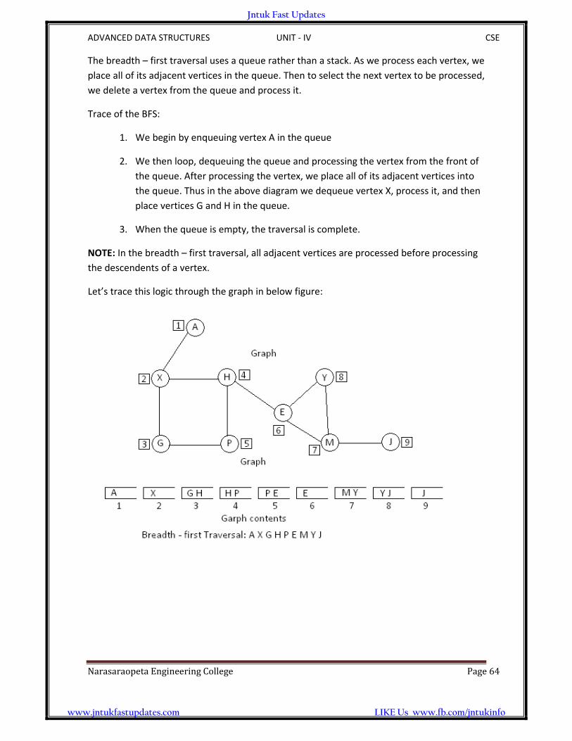
The breadth – first traversal uses a queue rather than a stack. As we process each vertex, we
place all of its adjacent vertices in the queue. Then to select the next vertex to be processed,
we delete a vertex from the queue and process it.
Trace of the BFS:
1. We begin by enqueuing vertex A in the queue
2. We then loop, dequeuing the queue and processing the vertex from the front of
the queue. After processing the vertex, we place all of its adjacent vertices into
the queue. Thus in the above diagram we dequeue vertex X, process it, and then
place vertices G and H in the queue.
3. When the queue is empty, the traversal is complete.
NOTE: In the breadth – first traversal, all adjacent vertices are processed before processing
the descendents of a vertex.
Let’s trace this logic through the graph in below figure:
Jntuk Fast Updates
www.jntukfastupdates.com LIKE Us www.fb.com/jntukinfo

ADVANCED DATA STRUCTURES UNIT ‐ IV CSE
NarasaraopetaEngineeringCollege Page65
Algorithms:
Depth – First Search:
Policy: Don’t push nodes twice
// non‐recursive, preorder, depth‐first search
void dfs (Node v) {
if (v == null)
return;
push(v);
while (stack is not empty) {
pop(v);
if (v has not yet been visited)
mark&visit(v);
for (each w adjacent to v)
if (w has not yet been visited && not yet stacked)
push(w);
} // while
} // dfs
Breadth‐First Search:
// non‐recursive, preorder, breadth‐first search
void bfs (Node v) {
if (v == null)
return;
enqueue(v);
while (queue is not empty) {
dequeue(v);
if (v has not yet been visited)
mark&visit(v);
for (each w adjacent to v)
if (w has not yet been visited && has not been queued)
enqueue(w);
} // while
} // bfs
Jntuk Fast Updates
www.jntukfastupdates.com LIKE Us www.fb.com/jntukinfo

ADVANCED DATA STRUCTURES UNIT ‐ IV CSE
NarasaraopetaEngineeringCollege Page66
Exercise problems:
Jntuk Fast Updates
www.jntukfastupdates.com LIKE Us www.fb.com/jntukinfo

ADVANCED DATA STRUCTURES UNIT ‐ V CSE
NarasaraopetaEngineeringCollege Page65
GRAPH ALGORITHMS
The trees are the special case of graphs. A tree may be defined as a connected graph
without any cycles.
A spanning tree of a graph is a sub ‐ graph which is basically a tree and it contains all the
vertices of graph containing no cycles.
Minimum – cost spanning tree:
A network is a graph whose lines are weighted. It is also known as a weighted graph. The
weight is an attribute of an edge. In an adjacency matrix, the weight is stored as the
intersection value. In an adjacency list, it is stored as the value in the adjacency linked list.
A minimum – cost spanning tree is a spanning tree in which the total weight of lines is
guaranteed to be the minimum of all possible trees in the graph.
Jntuk Fast Updates
www.jntukfastupdates.com LIKE Us www.fb.com/jntukinfo

ADVANCED DATA STRUCTURES UNIT ‐ V CSE
NarasaraopetaEngineeringCollege Page66
Example:
Before going into the types of algorithms which will apply to get the minimum spanning tree
of a graph
Let’s manually determine the minimum – cost spanning tree
We can start with any vertex. Because the vertex list is usually key sequenced,
Let’s start with A
The above example shows a graph and one of its minimum – cost spanning trees. Since the
identification of a minimum – cost spanning tree involves the selection of a subset of edges.
Applications of spanning tree:
1. Spanning trees are very important in designing efficient routing algorithms
2. Spanning trees are have wide applications in many areas such as network design
Jntuk Fast Updates
www.jntukfastupdates.com LIKE Us www.fb.com/jntukinfo

ADVANCED DATA STRUCTURES UNIT ‐ V CSE
NarasaraopetaEngineeringCollege Page67
There are two popular techniques to construct a minimum – cost spanning tree from a
weighted graph. One such method is known as Prim’s algorithm and another one is
Kruskal’s algorithm
Prim’s Algorithm:
The prim’s algorithm is implemented using the adjacency matrix of a graph. This matrix is
denoted by adjMatrix [i, j] where i and j operate from 0 to n‐1 for n – node weighted
undirected graph.
We can represent a weighted graph by an adjacency matrix to store the set of edges, an
entry (i, j) in an adjacency matrix contains information on the edge that goes from the
vertex i to the vertex j. each matrix entry contains the weight of the corresponding edge.
Let’s consider an example:
Now the sequence of below figures show the working of prim’s algorithm:
Jntuk Fast Updates
www.jntukfastupdates.com LIKE Us www.fb.com/jntukinfo

ADVANCED DATA STRUCTURES UNIT ‐ V CSE
NarasaraopetaEngineeringCollege Page68
Kruskal’s Algorithm:
Like Prim’s algorithm, Kruskal’s algorithm also constructs the minimum spanning tree of a
graph by adding edges to the spanning tree one – by – one. At all points during its
execution, the set of edges selected by prim’s algorithm forms exactly one tree, on the
other hand, the set of edges selected by Kruskal’s algorithm forms a forest of trees.
Let us consider a graph
Jntuk Fast Updates
www.jntukfastupdates.com LIKE Us www.fb.com/jntukinfo

ADVANCED DATA STRUCTURES UNIT ‐ V CSE
NarasaraopetaEngineeringCollege Page69
The edges of the graph are arranged in increasing order of weights as shown below. Initially
the spanning tree, T is empty. We select the edge with smallest weight and include it in T.
If selected edge creates a cycle, then it will be removed from T. We repeat these two steps
until the tree T contains n‐1 edges (where n is the number of vertices in the graph)
If the tree contains less than n‐1 edges and the edge list is empty, then no spanning tree is
possible for the graph
Jntuk Fast Updates
www.jntukfastupdates.com LIKE Us www.fb.com/jntukinfo
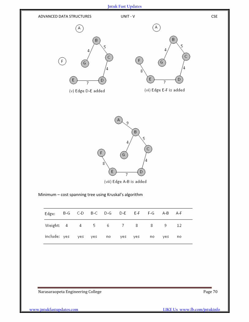
ADVANCED DATA STRUCTURES UNIT ‐ V CSE
NarasaraopetaEngineeringCollege Page70
Minimum – cost spanning tree using Kruskal’s algorithm
Jntuk Fast Updates
www.jntukfastupdates.com LIKE Us www.fb.com/jntukinfo
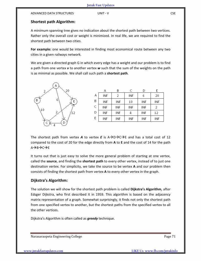
ADVANCED DATA STRUCTURES UNIT ‐ V CSE
NarasaraopetaEngineeringCollege Page71
Shortest path Algorithm:
A minimum spanning tree gives no indication about the shortest path between two vertices.
Rather only the overall cost or weight is minimized. In real life, we are required to find the
shortest path between two cities.
For example: one would be interested in finding most economical route between any two
cities in a given railways network.
We are given a directed graph G in which every edge has a weight and our problem is to find
a path from one vertex v to another vertex w such that the sum of the weights on the path
is as minimal as possible. We shall call such path a shortest path.
The shortest path from vertex A to vertex E is ADCE and has a total cost of 12
compared to the cost of 20 for the edge directly from A to E and the cost of 14 for the path
ABCE
It turns out that is just easy to solve the more general problem of starting at one vertex,
called the source, and finding the shortest path to every other vertex, instead of to just one
destination vertex. For simplicity, we take the source to be vertex A and our problem then
consists of finding the shortest path from vertex A to every other vertex in the graph.
Dijkstra’s Algorithm:
The solution we will show for the shortest path problem is called Dijkstra’s Algorithm, after
Edsger Dijkstra, who first described it in 1959. This algorithm is based on the adjacency
matrix representation of a graph. Somewhat surprisingly, it finds not only the shortest path
from one specified vertex to another, but the shortest paths from the specified vertex to all
the other vertices.
Dijkstra’s Algorithm is often called as greedy technique.
Jntuk Fast Updates
www.jntukfastupdates.com LIKE Us www.fb.com/jntukinfo
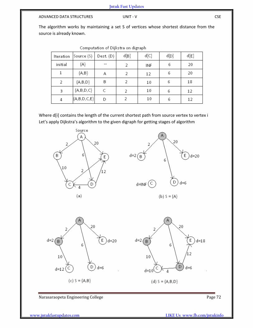
ADVANCED DATA STRUCTURES UNIT ‐ V CSE
NarasaraopetaEngineeringCollege Page72
The algorithm works by maintaining a set S of vertices whose shortest distance from the
source is already known.
Where d[i] contains the length of the current shortest path from source vertex to vertex i
Let’s apply Dijkstra’s algorithm to the given digraph for getting stages of algorithm
Jntuk Fast Updates
www.jntukfastupdates.com LIKE Us www.fb.com/jntukinfo

ADVANCED DATA STRUCTURES UNIT ‐ V CSE
NarasaraopetaEngineeringCollege Page73
Jntuk Fast Updates
www.jntukfastupdates.com LIKE Us www.fb.com/jntukinfo
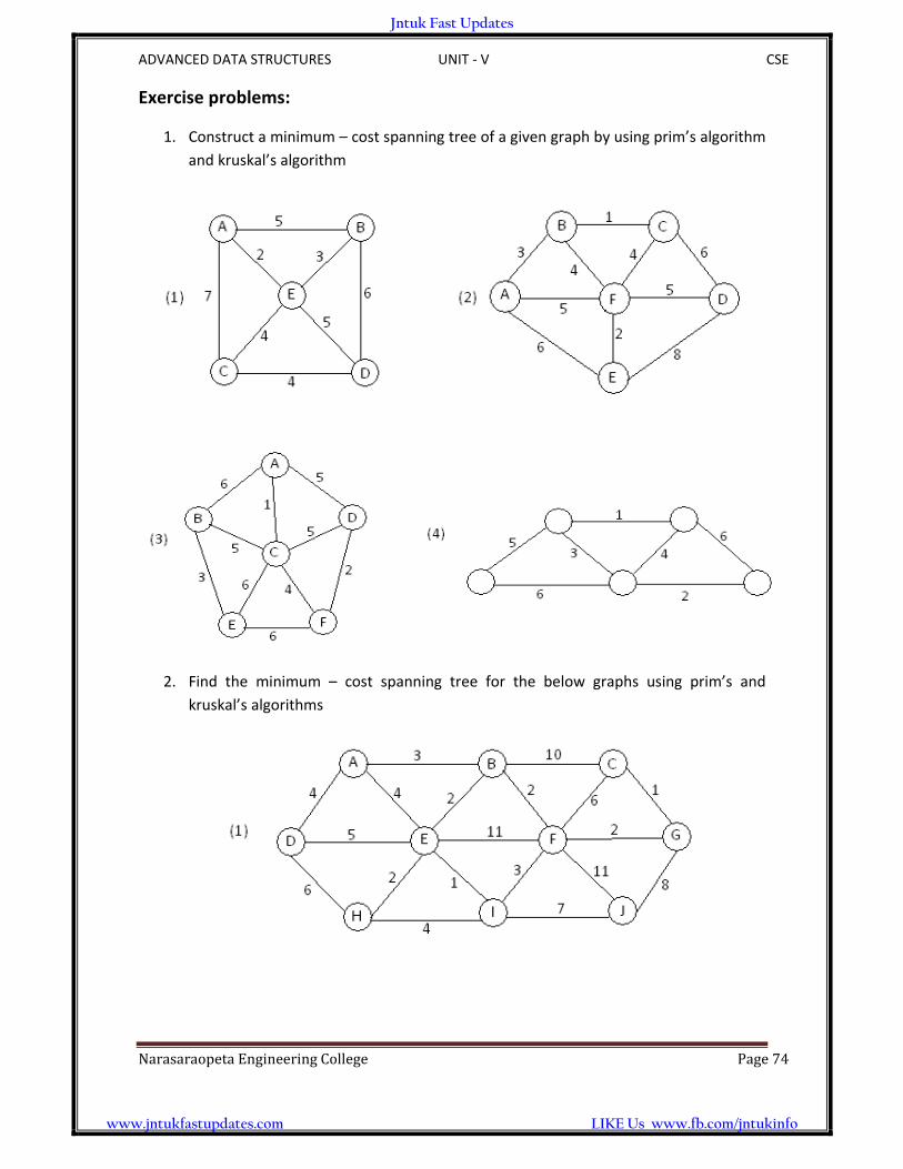
ADVANCED DATA STRUCTURES UNIT ‐ V CSE
NarasaraopetaEngineeringCollege Page74
Exercise problems:
1. Construct a minimum – cost spanning tree of a given graph by using prim’s algorithm
and kruskal’s algorithm
2. Find the minimum – cost spanning tree for the below graphs using prim’s and
kruskal’s algorithms
Jntuk Fast Updates
www.jntukfastupdates.com LIKE Us www.fb.com/jntukinfo

ADVANCED DATA STRUCTURES UNIT ‐ V CSE
NarasaraopetaEngineeringCollege Page75
3. Find the shortest path from A to all other vertices using Dijkstra’s algorithm for the
graph as shown below
4. Find the shortest path by using Dijkstra’s algorithm on the following edge weighted
directed graph with the vertex P as the source
Jntuk Fast Updates
www.jntukfastupdates.com LIKE Us www.fb.com/jntukinfo