adsorption and ion exchange - indian institute of...
TRANSCRIPT
DESIGN CONCEPTSIntroduction . . . . . . . . . . . . . . . . . . . . . . . . . . . . . . . . . . . . . . . . . . . . . . . 16-4Design Strategy. . . . . . . . . . . . . . . . . . . . . . . . . . . . . . . . . . . . . . . . . . . . . 16-5
Characterization of Equilibria . . . . . . . . . . . . . . . . . . . . . . . . . . . . . . . 16-5Adsorbent/Ion Exchanger Selection . . . . . . . . . . . . . . . . . . . . . . . . . . 16-5Fixed-Bed Behavior . . . . . . . . . . . . . . . . . . . . . . . . . . . . . . . . . . . . . . . 16-6Cycles . . . . . . . . . . . . . . . . . . . . . . . . . . . . . . . . . . . . . . . . . . . . . . . . . . 16-7Practical Aspects . . . . . . . . . . . . . . . . . . . . . . . . . . . . . . . . . . . . . . . . . . 16-7
ADSORBENTS AND ION EXCHANGERSClassifications and Characterizations. . . . . . . . . . . . . . . . . . . . . . . . . . . . 16-8
Adsorbents . . . . . . . . . . . . . . . . . . . . . . . . . . . . . . . . . . . . . . . . . . . . . . 16-8Ion Exchangers . . . . . . . . . . . . . . . . . . . . . . . . . . . . . . . . . . . . . . . . . . . 16-8
Physical Properties . . . . . . . . . . . . . . . . . . . . . . . . . . . . . . . . . . . . . . . . . . 16-9
SORPTION EQUILIBRIUMGeneral Considerations . . . . . . . . . . . . . . . . . . . . . . . . . . . . . . . . . . . . . . 16-11
Forces . . . . . . . . . . . . . . . . . . . . . . . . . . . . . . . . . . . . . . . . . . . . . . . . . . 16-11Surface Excess . . . . . . . . . . . . . . . . . . . . . . . . . . . . . . . . . . . . . . . . . . . 16-11Classification of Isotherms by Shape . . . . . . . . . . . . . . . . . . . . . . . . . . 16-11Categorization of Equilibrium Models . . . . . . . . . . . . . . . . . . . . . . . . 16-12Heterogeneity . . . . . . . . . . . . . . . . . . . . . . . . . . . . . . . . . . . . . . . . . . . . 16-12Isosteric Heat of Adsorption . . . . . . . . . . . . . . . . . . . . . . . . . . . . . . . . 16-12Experiments . . . . . . . . . . . . . . . . . . . . . . . . . . . . . . . . . . . . . . . . . . . . . 16-12Dimensionless Concentration Variables . . . . . . . . . . . . . . . . . . . . . . . 16-12
Single Component or Exchange. . . . . . . . . . . . . . . . . . . . . . . . . . . . . . . . 16-12Flat-Surface Isotherm Equations. . . . . . . . . . . . . . . . . . . . . . . . . . . . . 16-13Pore-Filling Isotherm Equations . . . . . . . . . . . . . . . . . . . . . . . . . . . . . 16-13Ion Exchange . . . . . . . . . . . . . . . . . . . . . . . . . . . . . . . . . . . . . . . . . . . . 16-13Donnan Uptake. . . . . . . . . . . . . . . . . . . . . . . . . . . . . . . . . . . . . . . . . . . 16-14Separation Factor . . . . . . . . . . . . . . . . . . . . . . . . . . . . . . . . . . . . . . . . . 16-14
Multiple Components or Exchanges . . . . . . . . . . . . . . . . . . . . . . . . . . . . 16-15Adsorbed-Solution Theory . . . . . . . . . . . . . . . . . . . . . . . . . . . . . . . . . . 16-15Langmuir-Type Relations . . . . . . . . . . . . . . . . . . . . . . . . . . . . . . . . . . . 16-16Freundlich-Type Relations. . . . . . . . . . . . . . . . . . . . . . . . . . . . . . . . . . 16-16Equations of State. . . . . . . . . . . . . . . . . . . . . . . . . . . . . . . . . . . . . . . . . 16-16Ion Exchange—Stoichiometry . . . . . . . . . . . . . . . . . . . . . . . . . . . . . . . 16-16Mass Action. . . . . . . . . . . . . . . . . . . . . . . . . . . . . . . . . . . . . . . . . . . . . . 16-16Constant Separation-Factor Treatment . . . . . . . . . . . . . . . . . . . . . . . . 16-16
CONSERVATION EQUATIONSMaterial Balances . . . . . . . . . . . . . . . . . . . . . . . . . . . . . . . . . . . . . . . . . . . 16-17Energy Balance. . . . . . . . . . . . . . . . . . . . . . . . . . . . . . . . . . . . . . . . . . . . . 16-17
RATE AND DISPERSION FACTORSTransport and Dispersion Mechanisms . . . . . . . . . . . . . . . . . . . . . . . . . . 16-18
Intraparticle Transport Mechanisms . . . . . . . . . . . . . . . . . . . . . . . . . . 16-18Extraparticle Transport and Dispersion Mechanisms. . . . . . . . . . . . . 16-18Heat Transfer . . . . . . . . . . . . . . . . . . . . . . . . . . . . . . . . . . . . . . . . . . . . 16-18
Intraparticle Mass Transfer . . . . . . . . . . . . . . . . . . . . . . . . . . . . . . . . . . . 16-18Pore Diffusion. . . . . . . . . . . . . . . . . . . . . . . . . . . . . . . . . . . . . . . . . . . . 16-19Solid Diffusion . . . . . . . . . . . . . . . . . . . . . . . . . . . . . . . . . . . . . . . . . . . 16-19Combined Pore and Solid Diffusion . . . . . . . . . . . . . . . . . . . . . . . . . . 16-20
External Mass Transfer. . . . . . . . . . . . . . . . . . . . . . . . . . . . . . . . . . . . . . . 16-20Axial Dispersion in Packed Beds . . . . . . . . . . . . . . . . . . . . . . . . . . . . . . . 16-20Rate Equations . . . . . . . . . . . . . . . . . . . . . . . . . . . . . . . . . . . . . . . . . . . . . 16-21
General Component Balance . . . . . . . . . . . . . . . . . . . . . . . . . . . . . . . . 16-21Linear Driving Force Approximation . . . . . . . . . . . . . . . . . . . . . . . . . 16-22Combined Intraparticle Resistances . . . . . . . . . . . . . . . . . . . . . . . . . . 16-22Overall Resistance . . . . . . . . . . . . . . . . . . . . . . . . . . . . . . . . . . . . . . . . 16-23Axial Dispersion Effects . . . . . . . . . . . . . . . . . . . . . . . . . . . . . . . . . . . . 16-24Rapid Adsorption-Desorption Cycles . . . . . . . . . . . . . . . . . . . . . . . . . 16-24Determination of Controlling Rate Factor . . . . . . . . . . . . . . . . . . . . . 16-24
16-1
Section 16
Adsorption and Ion Exchange
M. Douglas LeVan, Ph.D., Centennial Professor, Department of Chemical Engineering,Vanderbilt University; Member, American Institute of Chemical Engineers, American ChemicalSociety, International Adsorption Society. (Section Editor)
Giorgio Carta, Ph.D., Professor, Department of Chemical Engineering, University of Virginia; Member, American Institute of Chemical Engineers, American Chemical Society,International Adsorption Society.
Carmen M. Yon, M.S., Development Associate, UOP, Des Plaines, IL; Member, AmericanInstitute of Chemical Engineers. (Process Cycles, Equipment)
BATCH ADSORPTIONExternal Mass-Transfer Control. . . . . . . . . . . . . . . . . . . . . . . . . . . . . . . . 16-26Solid Diffusion Control . . . . . . . . . . . . . . . . . . . . . . . . . . . . . . . . . . . . . . 16-26Pore Diffusion Control . . . . . . . . . . . . . . . . . . . . . . . . . . . . . . . . . . . . . . . 16-28Combined Resistances . . . . . . . . . . . . . . . . . . . . . . . . . . . . . . . . . . . . . . . 16-28
Parallel Pore and Solid Diffusion Control . . . . . . . . . . . . . . . . . . . . . . 16-29External Mass Transfer and Intraparticle Diffusion Control . . . . . . . 16-29Bidispersed Particles . . . . . . . . . . . . . . . . . . . . . . . . . . . . . . . . . . . . . . 16-29
FIXED-BED TRANSITIONSDimensionless System . . . . . . . . . . . . . . . . . . . . . . . . . . . . . . . . . . . . . . . 16-30Local Equilibrium Theory . . . . . . . . . . . . . . . . . . . . . . . . . . . . . . . . . . . . 16-30
Single Transition System . . . . . . . . . . . . . . . . . . . . . . . . . . . . . . . . . . . 16-30Multiple Transition System . . . . . . . . . . . . . . . . . . . . . . . . . . . . . . . . . 16-31Extensions . . . . . . . . . . . . . . . . . . . . . . . . . . . . . . . . . . . . . . . . . . . . . . . 16-31
Constant Pattern Behavior for Favorable Isotherms . . . . . . . . . . . . . . . 16-32Asymptotic Solution . . . . . . . . . . . . . . . . . . . . . . . . . . . . . . . . . . . . . . . 16-34Breakthrough Behavior for Axial Dispersion. . . . . . . . . . . . . . . . . . . . 16-36Extensions . . . . . . . . . . . . . . . . . . . . . . . . . . . . . . . . . . . . . . . . . . . . . . . 16-36
Square Root Spreading for Linear Isotherms . . . . . . . . . . . . . . . . . . . . . 16-36Complete Solution for Reaction Kinetics . . . . . . . . . . . . . . . . . . . . . . . . 16-37Numerical Methods and Characterization of Wave Shape . . . . . . . . . . . 16-37
CHROMATOGRAPHYClassification . . . . . . . . . . . . . . . . . . . . . . . . . . . . . . . . . . . . . . . . . . . . . . . 16-38
Modes of Operation . . . . . . . . . . . . . . . . . . . . . . . . . . . . . . . . . . . . . . . 16-38Elution Chromatography . . . . . . . . . . . . . . . . . . . . . . . . . . . . . . . . . . . 16-38Frontal Analysis . . . . . . . . . . . . . . . . . . . . . . . . . . . . . . . . . . . . . . . . . . 16-39Displacement Development . . . . . . . . . . . . . . . . . . . . . . . . . . . . . . . . 16-39
Characterization of Experimental Chromatograms . . . . . . . . . . . . . . . . 16-40Method of Moments. . . . . . . . . . . . . . . . . . . . . . . . . . . . . . . . . . . . . . . 16-40Approximate Methods . . . . . . . . . . . . . . . . . . . . . . . . . . . . . . . . . . . . . 16-40Tailing Peaks . . . . . . . . . . . . . . . . . . . . . . . . . . . . . . . . . . . . . . . . . . . . . 16-41Resolution . . . . . . . . . . . . . . . . . . . . . . . . . . . . . . . . . . . . . . . . . . . . . . . 16-41
Prediction of Chromatographic Behavior . . . . . . . . . . . . . . . . . . . . . . . . 16-42Isocratic Elution . . . . . . . . . . . . . . . . . . . . . . . . . . . . . . . . . . . . . . . . . . 16-42Concentration Profiles . . . . . . . . . . . . . . . . . . . . . . . . . . . . . . . . . . . . . 16-43
Linear Gradient Elution. . . . . . . . . . . . . . . . . . . . . . . . . . . . . . . . . . . . 16-44Displacement Development . . . . . . . . . . . . . . . . . . . . . . . . . . . . . . . . 16-44
Design for Trace Solute Separations . . . . . . . . . . . . . . . . . . . . . . . . . . . . 16-47
PROCESS CYCLESGeneral Concepts . . . . . . . . . . . . . . . . . . . . . . . . . . . . . . . . . . . . . . . . . . . 16-48Temperature Swing Adsorption . . . . . . . . . . . . . . . . . . . . . . . . . . . . . . . . 16-48
Other Cycle Steps . . . . . . . . . . . . . . . . . . . . . . . . . . . . . . . . . . . . . . . . . 16-49Applications. . . . . . . . . . . . . . . . . . . . . . . . . . . . . . . . . . . . . . . . . . . . . . 16-49
Pressure-Swing Adsorption . . . . . . . . . . . . . . . . . . . . . . . . . . . . . . . . . . . 16-49Other Cycle Steps . . . . . . . . . . . . . . . . . . . . . . . . . . . . . . . . . . . . . . . . . 16-50Applications. . . . . . . . . . . . . . . . . . . . . . . . . . . . . . . . . . . . . . . . . . . . . . 16-50
Purge/Concentration Swing Adsorption . . . . . . . . . . . . . . . . . . . . . . . . . 16-51Inert Purge . . . . . . . . . . . . . . . . . . . . . . . . . . . . . . . . . . . . . . . . . . . . . . 16-51Displacement Purge . . . . . . . . . . . . . . . . . . . . . . . . . . . . . . . . . . . . . . . 16-51Chromatography . . . . . . . . . . . . . . . . . . . . . . . . . . . . . . . . . . . . . . . . . . 16-52
Ion Exchange . . . . . . . . . . . . . . . . . . . . . . . . . . . . . . . . . . . . . . . . . . . . . . 16-52Parametric Pumping. . . . . . . . . . . . . . . . . . . . . . . . . . . . . . . . . . . . . . . . . 16-53
Temperature . . . . . . . . . . . . . . . . . . . . . . . . . . . . . . . . . . . . . . . . . . . . . 16-55Pressure. . . . . . . . . . . . . . . . . . . . . . . . . . . . . . . . . . . . . . . . . . . . . . . . . 16-55
Other Adsorption Cycles . . . . . . . . . . . . . . . . . . . . . . . . . . . . . . . . . . . . . 16-55Steam. . . . . . . . . . . . . . . . . . . . . . . . . . . . . . . . . . . . . . . . . . . . . . . . . . . 16-55Energy Applications . . . . . . . . . . . . . . . . . . . . . . . . . . . . . . . . . . . . . . . 16-55Energy Conservation Techniques . . . . . . . . . . . . . . . . . . . . . . . . . . . . 16-55Process Selection . . . . . . . . . . . . . . . . . . . . . . . . . . . . . . . . . . . . . . . . . 16-56
EQUIPMENTAdsorption. . . . . . . . . . . . . . . . . . . . . . . . . . . . . . . . . . . . . . . . . . . . . . . . . 16-56
General Design . . . . . . . . . . . . . . . . . . . . . . . . . . . . . . . . . . . . . . . . . . . 16-56Adsorber Vessel. . . . . . . . . . . . . . . . . . . . . . . . . . . . . . . . . . . . . . . . . . . 16-56Regeneration Equipment. . . . . . . . . . . . . . . . . . . . . . . . . . . . . . . . . . . 16-58Cycle Control . . . . . . . . . . . . . . . . . . . . . . . . . . . . . . . . . . . . . . . . . . . . 16-59Continuous Countercurrent Systems. . . . . . . . . . . . . . . . . . . . . . . . . . 16-60Continuous Cross-Flow Systems . . . . . . . . . . . . . . . . . . . . . . . . . . . . . 16-61Simulated Continuous Countercurrent Systems. . . . . . . . . . . . . . . . . 16-62
Ion Exchange . . . . . . . . . . . . . . . . . . . . . . . . . . . . . . . . . . . . . . . . . . . . . . 16-64
16-2 ADSORPTION AND ION EXCHANGE

ADSORPTION AND ION EXCHANGE 16-3
a specific external surface area per unit bed volume, m2/m3
av surface area per unit particle volume, m2/m3 particleA surface area of solid, m2/kgAs chromatography peak asymmetry factorb correction factor for resistances in seriesc fluid-phase concentration, mol/m3 fluidcp pore fluid-phase concentration, mol/m3
c s fluid-phase concentration at particle surface, mol/m3
C°pf ideal gas heat capacity, J/(mol K)Cs heat capacity of sorbent solid, J/(kg K)dp particle diameter, mD fluid-phase diffusion coefficient, m2/sDe equivalent diffusion coefficient, m2/sDL axial dispersion coefficient, m2/sDp pore diffusion coefficient, m2/sDs adsorbed-phase (solid, surface, particle, or micropore) diffusion
coefficient, m2/sD0 diffusion coefficient corrected for thermodynamic driving force, m2/sD ionic self-diffusion coefficient, m2/sF fractional approach to equilibriumFv volumetric flow rate, m3/sh enthalpy, J/mol;
reduced height equivalent to theoretical platehtu reduced height equivalent to a transfer unitHETP height equivalent to theoretical plate, mHTU height equivalent to a transfer unit, mJ mass-transfer flux relative to molar average velocity, mol/(m2·s);
J functionk rate coefficient, s−1
ka forward rate constant for reaction kinetics, m3/(mol s)kc rate coefficient based on fluid-phase concentration driving force,
m3/(kg·s)kf external mass-transfer coefficient, m/skn rate coefficient based on adsorbed-phase concentration driving
force, s−1
k′ retention factorK isotherm parameterKc molar selectivity coefficientK′ rational selectivity coefficientL bed length, mm isotherm exponentMr molecular weight, kg/kmolMs mass of adsorbent, kgn adsorbed-phase concentration, mol/kg adsorbentns ion-exchange capacity, g-equiv/kgN number of transfer or reaction units; kfaL /(εvref) for external mass
transfer; 15(1 − ε)εpDpL/(εvrefRp2) for pore diffusion;
15ΛDsL /(εvrefRp2) for solid diffusion; knΛL /(εvref) for linear driving-
force approximation; kacrefΛL /[(1 − R)εvref] for reaction kineticsNp number of theoretical platesNPe vrefL /DL, bed Peclet number (number of dispersion units)p partial pressure, PaP pressure, PaPe particle-based Peclet number, dpv/DL
qst isosteric heat of adsorption, J/molQi amount of component i injected with feed, molr, R separation factor;
particle radial coordinate, mrc column internal radius, mrm hydrodynamic radius of molecule, mrp particle radius, mrpore pore radius, mrs radius of subparticles, mℜ gas constant, Pa⋅m3/(mol K)Re Reynolds number based on particle diameter, dpεv/νs UNILAN isotherm parameterSc Schmidt number, ν/DSh Sherwood number, kf dp /D
t time, stc cycle time, stf feed time, str chromatographic retention time, sT absolute temperature, Kuf fluid-phase internal energy, J/molus, usol stationary-phase and sorbent solid internal energy, J/kgv interstitial velocity, m/sVf extraparticle fluid volume, m3
W volume adsorbed as liquid, m3;baseline width of chromatographic peak, s
x adsorbed-phase mole fraction;particle coordinate, m
y fluid-phase mole fractionz bed axial coordinate, m; ionic valence
Greek letters
α separation factorβ scaling factor in Polanyi-based models;
slope in gradient elution chromatography∆ peak width at half height, sε void fraction of packing (extraparticle);
adsorption potential in Polanyi model, J/molεp particle porosity (intraparticle void fraction)εb total bed voidage (inside and outside particles)γ activity coefficientΓ surface excess, mol/m2
κ Boltzmann constantΛ partition ratioΛ∞ ultimate fraction of solute adsorbed in batchµ fluid viscosity, kg/(m s)µ0 zero moment, mol s/m3
µ1 first moment, sν kinematic viscosity, m2/sΩ cycle-time dependent LDF coefficientϕ volume fraction or mobile-phase modulator concentration, mol/m3
π spreading pressure, N/mψ LDF correction factorΨ mechanism parameter for combined resistancesρ subparticle radial coordinate, mρb bulk density of packing, kg/m3
ρp particle density, kg/m3
ρs skeletal particle density, kg/m3
σ2 second central moment, s2
τ dimensionless timeτ1 throughput parameterτp tortuosity factorξ particle dimensionless radial coordinateζ dimensionless bed axial coordinate
Subscripts
a adsorbed phasef fluid phasei, j component indextot total
Superscripts
− an averaged concentration^ a combination of averaged concentrations* dimensionless concentration variablee equilibriumref references saturationSM service markTM trademark0 initial fluid concentration in batch0′ initial adsorbed-phase concentration in batch∞ final state approached in batch
Nomenclature and Units
GENERAL REFERENCES1. Adamson, Physical Chemistry of Surfaces, Wiley, New York, 1990.2. Barrer, Zeolites and Clay Minerals as Adsorbents and Molecular Sieves,
Academic Press, New York, 1978.3. Breck, D. W., Zeolite Molecular Sieves, Wiley, New York, 1974.4. Cheremisinoff and Ellerbusch, Carbon Adsorption Handbook, Ann Arbor
Science, Ann Arbor, 1978.5. Dorfner (ed.), Ion Exchangers, W. deGruyter, Berlin, 1991.6. Dyer, An Introduction to Zeolite Molecular Sieves, Wiley, New York, 1988.7. EPA, Process Design Manual for Carbon Adsorption, U.S. Envir. Protect.
Agency., Cincinnati, 1973.8. Gembicki, Oroskar, and Johnson, “Adsorption, Liquid Separation” in Kirk-
Othmer Encyclopedia of Chemical Technology, 4th ed., Wiley, 1991.9. Guiochon, Golsham-Shirazi, and Katti, Fundamentals of Preparative and
Nonlinear Chromatography, Academic Press, Boston, Massachusetts, 1994.
10. Gregg and Sing, Adsorption, Surface Area and Porosity, Academic Press,New York, 1982.
11. Helfferich, Ion Exchange, McGraw-Hill, New York, 1962; reprinted byUniversity Microfilms International, Ann Arbor, Michigan.
12. Helfferich and Klein, Multicomponent Chromatography, Marcel Dekker,New York, 1970.
13. Jaroniec and Madey, Physical Adsorption on Heterogeneous Solids, Else-vier, New York, 1988.
14. Karge and Ruthven, Diffusion in Zeolites and Other Microporous Solids,Wiley, New York, 1992.
15. Keller, Anderson, and Yon, “Adsorption” in Rousseau (ed.), Handbook ofSeparation Process Technology, Wiley-Interscience, New York, 1987.
16. Rhee, Aris, and Amundson, First-Order Partial Differential Equations:
Volume 1. Theory and Application of Single Equations; Volume 2. Theoryand Application of Hyperbolic Systems of Quasi-Linear Equations, Pren-tice Hall, Englewood Cliffs, New Jersey, 1986, 1989.
17. Rodrigues, LeVan, and Tondeur (eds.), Adsorption: Science and Technol-ogy, Kluwer Academic Publishers, Dordrecht, The Netherlands, 1989.
18. Rudzinski and Everett, Adsorption of Gases on Heterogeneous Surfaces,Academic Press, San Diego, 1992.
19. Ruthven, Principles of Adsorption and Adsorption Processes, Wiley, NewYork, 1984.
20. Ruthven, Farooq, and Knaebel, Pressure Swing Adsorption, VCH Pub-lishers, New York, 1994.
21. Sherman and Yon, “Adsorption, Gas Separation” in Kirk-Othmer Encyclo-pedia of Chemical Technology, 4th ed., Wiley, 1991.
22. Streat and Cloete, “Ion Exchange,” in Rousseau (ed.), Handbook of Sepa-ration Process Technology, Wiley, New York, 1987.
23. Suzuki, Adsorption Engineering, Elsevier, Amsterdam, 1990.24. Tien, Adsorption Calculations and Modeling, Butterworth-Heinemann,
Newton, Massachusetts, 1994.25. Valenzuela and Myers, Adsorption Equilibrium Data Handbook, Prentice
Hall, Englewood Cliffs, New Jersey, 1989.26. Vermeulen, LeVan, Hiester, and Klein, “Adsorption and Ion Exchange” in
Perry, R. H. and Green, D. W. (eds.), Perry’s Chemical Engineers’ Hand-book (6th ed.), McGraw-Hill, New York, 1984.
27. Wankat, Large-Scale Adsorption and Chromatography, CRC Press, BocaRaton, Florida, 1986.
28. Yang, Gas Separation by Adsorption Processes, Butterworth, Stoneham,Massachusetts, 1987.
29. Young and Crowell, Physical Adsorption of Gases, Butterworths, London,1962.
INTRODUCTION
Adsorption and ion exchange share so many common features inregard to application in batch and fixed-bed processes that they can begrouped together as sorption for a unified treatment. These processesinvolve the transfer and resulting equilibrium distribution of one ormore solutes between a fluid phase and particles. The partitioning ofa single solute between fluid and sorbed phases or the selectivity of asorbent towards multiple solutes makes it possible to separate solutesfrom a bulk fluid phase or from one another.
This section treats batch and fixed-bed operations and reviewsprocess cycles and equipment. As the processes indicate, fixed-bedoperation with the sorbent in granule, bead, or pellet form is the pre-dominant way of conducting sorption separations and purifications.Although the fixed-bed mode is highly useful, its analysis is complex.Therefore, fixed beds including chromatographic separations aregiven primary attention here with respect to both interpretation andprediction.
Adsorption involves, in general, the accumulation (or depletion) ofsolute molecules at an interface (including gas-liquid interfaces, as infoam fractionation, and liquid-liquid interfaces, as in detergency).Here we consider only gas-solid and liquid-solid interfaces, withsolute distributed selectively between the fluid and solid phases. Theaccumulation per unit surface area is small; thus, highly porous solidswith very large internal area per unit volume are preferred. Adsorbentsurfaces are often physically and/or chemically heterogeneous, andbonding energies may vary widely from one site to another. We seek topromote physical adsorption or physisorption, which involves van derWaals forces (as in vapor condensation), and retard chemical adsorp-tion or chemisorption, which involves chemical bonding (and oftendissociation, as in catalysis). The former is well suited for a regenera-
ble process, while the latter generally destroys the capacity of theadsorbent.
Adsorbents are natural or synthetic materials of amorphous ormicrocrystalline structure. Those used on a large scale, in order ofsales volume, are activated carbon, molecular sieves, silica gel, andactivated alumina [Keller et al., gen. refs.].
Ion exchange usually occurs throughout a polymeric solid, the solidbeing of gel-type, which dissolves some fluid-phase solvent, or trulyporous. In ion exchange, ions of positive charge in some cases(cations) and negative charge in others (anions) from the fluid (usuallyan aqueous solution) replace dissimilar ions of the same charge ini-tially in the solid. The ion exchanger contains permanently boundfunctional groups of opposite charge-type (or, in special cases, notablyweak-base exchangers act as if they do). Cation-exchange resins gen-erally contain bound sulfonic acid groups; less commonly, thesegroups are carboxylic, phosphonic, phosphinic, and so on. Anionicresins involve quaternary ammonium groups (strongly basic) or otheramino groups (weakly basic).
Most ion exchangers in large-scale use are based on syntheticresins—either preformed and then chemically reacted, as for poly-styrene, or formed from active monomers (olefinic acids, amines, orphenols). Natural zeolites were the first ion exchangers, and both nat-ural and synthetic zeolites are in use today.
Ion exchange may be thought of as a reversible reaction involvingchemically equivalent quantities. A common example for cationexchange is the familiar water-softening reaction
Ca++ + 2NaRA CaR2 + 2Na+
where R represents a stationary univalent anionic site in the polyelec-trolyte network of the exchanger phase.
16-4
DESIGN CONCEPTS

Table 16-1 classifies sorption operations by the type of interactionand the basis for the separation. In addition to the normal sorptionoperations of adsorption and ion exchange, some other similar separa-tions are included. Applications are discussed in this section in“Process Cycles.”
Example 1: Surface Area and Pore Volume of Adsorbent Asimple example will show the extent of internal area in a typical granular adsor-bent. A fixed bed is packed with particles of a porous adsorbent material. Thebulk density of the packing is 500 kg/m3, and the interparticle void fraction is0.40. The intraparticle porosity is 0.50, with two-thirds of this in cylindricalpores of diameter 1.4 nm and the rest in much larger pores. Find the surfacearea of the adsorbent and, if solute has formed a complete monomolecular layer0.3 nm thick inside the pores, determine the percent of the particle volume andthe percent of the total bed volume filled with adsorbate.
From surface area to volume ratio considerations, the internal area is practi-cally all in the small pores. One gram of the adsorbent occupies 2 cm3 as packedand has 0.4 cm3 in small pores, which gives a surface area of 1150 m2/g (or about1 mi2 per 5 lb or 6.3 mi2/ft3 of packing). Based on the area of the annular regionfilled with adsorbate, the solute occupies 22.5 percent of the internal pore vol-ume and 13.5 percent of the total packed-bed volume.
DESIGN STRATEGY
The design of sorption systems is based on a few underlying princi-ples. First, knowledge of sorption equilibrium is required. This equi-librium, between solutes in the fluid phase and the solute-enrichedphase of the solid, supplants what in most chemical engineering sepa-rations is a fluid-fluid equilibrium. The selection of the sorbent mate-rial with an understanding of its equilibrium properties (i.e., capacityand selectivity as a function of temperature and component concen-trations) is of primary importance. Second, because sorption opera-tions take place in batch, in fixed beds, or in simulated moving beds,the processes have dynamical character. Such operations generally donot run at steady state, although such operation may be approached ina simulated moving bed. Fixed-bed processes often approach a peri-odic condition called a periodic state or cyclic steady state, with sev-eral different feed steps constituting a cycle. Thus, some knowledge ofhow transitions travel through a bed is required. This introduces bothtime and space into the analysis, in contrast to many chemical engi-neering operations that can be analyzed at steady state with only a spa-tial dependence. For good design, it is crucial to understand fixed-bedperformance in relation to adsorption equilibrium and rate behavior.Finally, many practical aspects must be included in design so that aprocess starts up and continues to perform well, and that it is not sooverdesigned that it is wasteful. While these aspects are process-specific, they include an understanding of dispersive phenomena atthe bed scale and, for regenerative processes, knowledge of agingcharacteristics of the sorbent material, with consequent changes insorption equilibrium.
Characterization of Equilibria Phase equilibrium betweenfluid and sorbed phases for one or many components in adsorption ortwo or more species in ion exchange is usually the single most impor-tant factor affecting process performance. In most processes, it ismuch more important than mass and heat transfer rates; a doubling ofthe stoichiometric capacity of a sorbent or a significant change in theshape of an isotherm would almost always have a greater impact onprocess performance than a doubling of transfer rates.
A difference between adsorption and ion exchange with completelyionized resins is indicated in the variance of the systems. In adsorp-tion, part of the solid surface or pore volume is vacant. This diminishesas the fluid-phase concentration of solute increases. In contrast, forion exchange the sorbent has a fixed total capacity and merelyexchanges solutes while conserving charge. Variance is defined as thenumber of independent concentration variables in a sorption systemat equilibrium—that is, variables that one can change separately andthereby control the values of all others. Thus, it also equals the differ-ence between the total number of concentration variables and thenumber of independent relations connecting them. Numerous casesarise in which ion exchange is accompanied by chemical reaction(neutralization or precipitation, in particular), or adsorption is accom-panied by evolution of sensible heat. The concept of variance helpsgreatly to assure correct interpretations and predictions.
The working capacity of a sorbent depends on fluid concentrationsand temperatures. Graphical depiction of sorption equilibrium forsingle component adsorption or binary ion exchange (monovariance)is usually in the form of isotherms [ni = ni(ci) or ni(pi) at constant T] orisosteres [pi = pi(T) at constant ni]. Representative forms are shown inFig. 16-1. An important dimensionless group dependent on adsorp-tion equilibrium is the partition ratio (see Eq. 16-125), which is ameasure of the relative affinities of the sorbed and fluid phases forsolute.
Historically, isotherms have been classified as favorable (concavedownward) or unfavorable (concave upward). These terms refer tothe spreading tendencies of transitions in fixed beds. A favorableisotherm gives a compact transition, whereas an unfavorable isothermleads to a broad one.
Example 2: Calculation of Variance In mixed-bed deionization ofa solution of a single salt, there are 8 concentration variables: 2 each for cation,anion, hydrogen, and hydroxide. There are 6 connecting relations: 2 for ionexchange and 1 for neutralization equilibrium, and 2 ion-exchanger and 1 solu-tion electroneutrality relations. The variance is therefore 8 − 6 = 2.
Adsorbent/Ion Exchanger Selection Guidelines for sorbentselection are different for regenerative and nonregenerative systems.For a nonregenerative system, one generally wants a high capacity anda strongly favorable isotherm for a purification and additionally highselectivity for a separation. For a regenerative system, high overallcapacity and selectivity are again desired, but needs for cost-effective
DESIGN CONCEPTS 16-5
TABLE 16-1 Classification of Sorptive Separations
Type of interaction Basis for separation Examples
Adsorption Equilibrium Numerous purification and recovery processes for gases and liquidsActivated carbon-based applicationsDesiccation using silica gels, aluminas, and zeolitesOxygen from air by PSA using 5A zeolite
Rate Nitrogen from air by PSA using carbon molecular sieveMolecular sieving Separation on n- and iso-parafins using 5A zeolite
Separation of xylenes using zeolite
Ion exchange (electrostatic) Equilibrium DeionizationWater softeningRare earth separationsRecovery and separation of pharmaceuticals (e.g., amino acids, proteins)
Ligand exchange Equilibrium Chromatographic separation of glucose-fructose mixtures with Ca-form resinsRemoval of heavy metals with chelating resinsAffinity chromatography
Solubility Equilibrium Partition chromatography
None (purely steric) Equilibrium partitioning in pores Size exclusion or gel permeation chromatography

regeneration leading to a reasonable working capacity influence whatis sought after in terms of isotherm shape. For separations by pressureswing adsorption (or vacuum pressure swing adsorption), generally onewants a linear to slightly favorable isotherm (although purifications canoperate economically with more strongly favorable isotherms). Tem-perature-swing adsorption usually operates with moderately to stronglyfavorable isotherms, in part because one is typically dealing with heav-ier solutes and these are adsorbed fairly strongly (e.g., organic solventson activated carbon and water vapor on zeolites). Exceptions exist,however; for example, water is adsorbed on silica gel and activated alumina only moderately favorably, with some isotherms showing un-favorable sections. Equilibria for ion exchange separations generallyvary from moderately favorable to moderately unfavorable; dependingon feed concentrations, the alternates often exist for the different steps of a regenerative cycle. Other factors in sorbent selection aremechanical and chemical stability, mass transfer characteristics, andcost.
Fixed-Bed Behavior The number of transitions occurring in afixed bed of initially uniform composition before it becomes saturatedby a constant composition feed stream is generally equal to the vari-ance of the system. This introductory discussion will be limited to sin-gle transition systems.
Methods for analysis of fixed-bed transitions are shown in Table 16-2. Local equilibrium theory is based solely of stoichiometric con-cerns and system nonlinearities. A transition becomes a “simple wave”(a gradual transition), a “shock” (an abrupt transition), or a combina-tion of the two. In other methods, mass-transfer resistances are incor-porated.
The asymptotic behavior of transitions under the influence of mass-
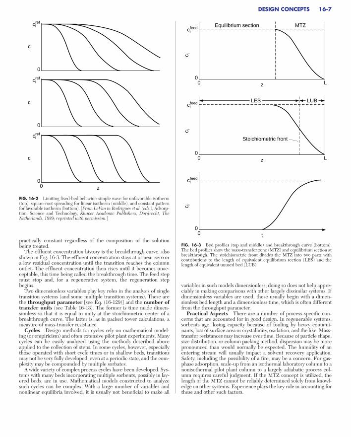
transfer resistances in long, “deep” beds is important. The three basicasymptotic forms are shown in Fig. 16-2. With an unfavorableisotherm, the breadth of the transition becomes proportional to the depth of bed it has passed through. For the linear isotherm, thebreadth becomes proportional to the square root of the depth. For the favorable isotherm, the transition approaches a constant breadthcalled a constant pattern.
Design of nonregenerative sorption systems and many regenerativeones often relies on the concept of the mass-transfer zone or MTZ,which closely resembles the constant pattern [Collins, Chem. Eng.Prog. Symp. Ser. No. 74, 63, 31 (1974); Keller et al., gen. refs.]. Thelength of this zone (depicted in Fig. 16-3) together with stoichiometrycan be used to predict accurately how long a bed can be utilized priorto breakthrough. Upstream of the mass-transfer zone, the adsorbent isin equilibrium with the feed. Downstream, the adsorbent is in its ini-tial state. Within the mass-transfer zone, the fluid-phase concentra-tion drops from the feed value to the initial, presaturation state.Equilibrium with the feed is not attained in this region. As a result,because an adsorption bed must typically be removed from serviceshortly after breakthrough begins, the full capacity of the bed is notutilized. Obviously, the broader that the mass-transfer zone is, thegreater will be the extent of unused capacity. Also shown in the figureis the length of the equivalent equilibrium section (LES) and thelength of equivalent unused bed (LUB). The length of the MTZ isdivided between these two.
Adsorption with strongly favorable isotherms and ion exchangebetween strong electrolytes can usually be carried out until most ofthe stoichiometric capacity of the sorbent has been utilized, corre-sponding to a thin MTZ. Consequently, the total capacity of the bed is
16-6 ADSORPTION AND ION EXCHANGE
Cold
00
Hotn i
ci or pi
ln p
i
Large ni
Small n
iI/T
FIG. 16-1 Isotherms (left) and isosteres (right). Isosteres plotted using these coordinates are nearlystraight parallel lines, with deviations caused by the dependence of the isosteric heat of adsorption on tem-perature and loading.
TABLE 16-2 Methods of Analysis of Fixed-Bed Transitions
Method Purpose Approximations
Local equilibrium theory Shows wave character—simple waves and shocks Mass and heat transfer very rapidUsually indicates best possible performance Dispersion usually neglectedBetter understanding If nonisothermal, then adiabatic
Mass-transfer zone Design based on stoichiometry and experience IsothermalMTZ length largely empiricalRegeneration often empirical
Constant pattern and Gives asymptotic transition shapes and upper bound on MTZ Deep bed with fully developed transitionrelated analyses
Full rate modeling Accurate description of transitions Various to fewAppropriate for shallow beds, with incomplete wave developmentGeneral numerical solutions by finite difference or collocation methods
practically constant regardless of the composition of the solutionbeing treated.
The effluent concentration history is the breakthrough curve, alsoshown in Fig. 16-3. The effluent concentration stays at or near zero ora low residual concentration until the transition reaches the columnoutlet. The effluent concentration then rises until it becomes unac-ceptable, this time being called the breakthrough time. The feed stepmust stop and, for a regenerative system, the regeneration stepbegins.
Two dimensionless variables play key roles in the analysis of singletransition systems (and some multiple transition systems). These arethe throughput parameter [see Eq. (16-129)] and the number oftransfer units (see Table 16-13). The former is time made dimen-sionless so that it is equal to unity at the stoichiometric center of abreakthrough curve. The latter is, as in packed tower calculations, ameasure of mass-transfer resistance.
Cycles Design methods for cycles rely on mathematical model-ing (or empiricism) and often extensive pilot plant experiments. Manycycles can be easily analyzed using the methods described aboveapplied to the collection of steps. In some cycles, however, especiallythose operated with short cycle times or in shallow beds, transitionsmay not be very fully developed, even at a periodic state, and the com-plexity may be compounded by multiple sorbates.
A wide variety of complex process cycles have been developed. Sys-tems with many beds incorporating multiple sorbents, possibly in lay-ered beds, are in use. Mathematical models constructed to analyzesuch cycles can be complex. With a large number of variables andnonlinear equilibria involved, it is usually not beneficial to make all
variables in such models dimensionless; doing so does not help appre-ciably in making comparisons with other largely dissimilar systems. Ifdimensionless variables are used, these usually begin with a dimen-sionless bed length and a dimensionless time, which is often differentfrom the throughput parameter.
Practical Aspects There are a number of process-specific con-cerns that are accounted for in good design. In regenerable systems,sorbents age, losing capacity because of fouling by heavy contami-nants, loss of surface area or crystallinity, oxidation, and the like. Mass-transfer resistances may increase over time. Because of particle shape,size distribution, or column packing method, dispersion may be morepronounced than would normally be expected. The humidity of anentering stream will usually impact a solvent recovery application.Safety, including the possibility of a fire, may be a concern. For gas-phase adsorption, scale-up from an isothermal laboratory column to anonisothermal pilot plant column to a largely adiabatic process col-umn requires careful judgment. If the MTZ concept is utilized, thelength of the MTZ cannot be reliably determined solely from knowl-edge on other systems. Experience plays the key role in accounting forthese and other such factors.
DESIGN CONCEPTS 16-7
0
ciref
ci
0
ciref
ci
00 z
ciref
ci
FIG. 16-2 Limiting fixed-bed behavior: simple wave for unfavorable isotherm(top), square-root spreading for linear isotherm (middle), and constant patternfor favorable isotherm (bottom). [From LeVan in Rodrigues et al. (eds.), Adsorp-tion: Science and Technology, Kluwer Academic Publishers, Dordrecht, TheNetherlands, 1989; reprinted with permission.]
00 Lz
cifeed
c ic i
c i
Equilibrium section MTZ
00 t
cifeed
00 Lz
cifeed
Stoichiometric front
LUBLES
FIG. 16-3 Bed profiles (top and middle) and breakthrough curve (bottom).The bed profiles show the mass-transfer zone (MTZ) and equilibrium section atbreakthrough. The stoichiometric front divides the MTZ into two parts withcontributions to the length of equivalent equilibrium section (LES) and thelength of equivalent unused bed (LUB).
CLASSIFICATIONS AND CHARACTERIZATIONS
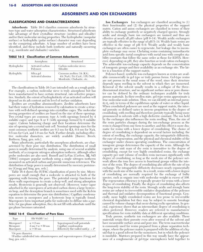
Adsorbents Table 16-3 classifies common adsorbents by struc-ture type and water adsorption characteristics. Structured adsorbentstake advantage of their crystalline structure (zeolites and silicalite)and/or their molecular sieving properties. The hydrophobic (nonpolarsurface) or hydrophilic (polar surface) character may vary dependingon the competing adsorbate. A large number of zeolites have beenidentified, and these include both synthetic and naturally occurring(e.g., mordenite and chabazite) varieties.
The classifications in Table 16-3 are intended only as a rough guide.For example, a carbon molecular sieve is truly amorphous but hasbeen manufactured to have certain structural, rate-selective proper-ties. Similarly, the extent of hydrophobicity of an activated carbon willdepend on its ash content and its level of surface oxidation.
Zeolites are crystalline aluminosilicates. Zeolitic adsorbents havehad their water of hydration removed by calcination to create a struc-ture with well-defined openings into crystalline cages. The molecularsieving properties of zeolites are based on the size of these openings.Two crystal types are common: type A (with openings formed by 4sodalite cages) and type X or Y (with openings formed by 6 sodalitecages). Cations balancing charge and their locations determine thesize of opening into a crystal unit cell. Nominal openings sizes for themost common synthetic zeolites are 0.3 nm for KA, 0.4 nm for NaA,0.5 nm for CaA, and 1.0 nm for NaX. Further details, including effec-tive molecular diameters, are widely available [Barrer; Breck;Ruthven; Yang, gen. refs.].
Many adsorbents, particularly the amorphous adsorbents, are char-acterized by their pore size distribution. The distribution of smallpores is usually determined by analysis, using one of several availablemethods, of a cryogenic nitrogen adsorption isotherm, although otherprobe molecules are also used. Russell and LeVan [Carbon, 32, 845(1994)] compare popular methods using a single nitrogen isothermmeasured on activated carbon and provide numerous references. Thedistribution of large pores is usually determined by mercury porisime-try [Gregg and Sing, gen. refs.].
Table 16-4 shows the IUPAC classification of pores by size. Micro-pores are small enough that a molecule is attracted to both of theopposing walls forming the pore. The potential energy functions forthese walls superimpose to create a deep well, and strong adsorptionresults. Hysteresis is generally not observed. (However, water vaporadsorbed in the micropores of activated carbon shows a large hystere-sis loop, and the desorption branch is sometimes used with the Kelvinequation to determine the pore size distribution.) Capillary condensa-tion occurs in mesopores and a hysteresis loop is typically found.Macropores form important paths for molecules to diffuse into a par-ticle; for gas-phase adsorption, they do not fill with adsorbate until thegas phase becomes saturated.
Ion Exchangers Ion exchangers are classified according to (1)their functionality and (2) the physical properties of the supportmatrix. Cation and anion exchangers are classified in terms of theirability to exchange positively or negatively charged species. Stronglyacidic and strongly basic ion exchangers are ionized and thus areeffective at nearly all pH values (pH 0–14). Weakly acidic exchangersare typically effective in the range of pH 5–14. Weakly basic resins areeffective in the range of pH 0–9. Weakly acidic and weakly basicexchangers are often easier to regenerate, but leakage due to incom-plete exchange may occur. Chelating resins containing iminodiaceticacid form specific metal complexes with metal ions with complex sta-bility constants that follow the same order as those for EDTA. How-ever, depending on pH, they also function as weak cation exchangers.The achievable ion-exchange capacity depends on the concentrationof ionogenic groups and their availability as an exchange site. The lat-ter is a function of the support matrix.
Polymer-based, synthetic ion-exchangers known as resins are avail-able commercially in gel type or truly porous forms. Gel-type resinsare not porous in the usual sense of the word, since their structuredepends upon swelling in the solvent in which they are immersed.Removal of the solvent usually results in a collapse of the three-dimensional structure, and no significant surface area or pore diame-ter can be defined by the ordinary techniques available for trulyporous materials. In their swollen state, gel-type resins approximate atrue molecular-scale solution. Thus, we can identify an internal poros-ity εp only in terms of the equilibrium uptake of water or other liquid.When crosslinked polymers are used as the support matrix, the inter-nal porosity so defined varies in inverse proportion to the degree ofcrosslinking, with swelling and therefore porosity typically being morepronounced in solvents with a high dielectric constant. The ion heldby the exchanger also influences the resin swelling. Thus, the size ofthe resin particles changes during the ion-exchange process as theresin is changed from one form to another, and this effect is more dra-matic for resins with a lower degree of crosslinking. The choice ofdegree of crosslinking is dependent on several factors including: theextent of swelling, the exchange capacity, the intraparticle diffusivity,the ease of regeneration, and the physical and chemical stability of theexchanger under chosen operating conditions. The concentration ofionogenic groups determines the capacity of the resin. Although thecapacity per unit mass of dry resin is insensitive to the degree ofcrosslinking, except for very highly crosslinked resins, the exchangecapacity per unit volume of swollen resin increases significantly withdegree of crosslinking, so long as the mesh size of the polymer net-work allows the ions free access to functional groups within the inte-rior of the resin. The degree of crosslinking also affects the rate of ionexchange. The intraparticle diffusivity decreases nearly exponentiallywith the mesh size of the matrix. As a result, resins with a lower degreeof crosslinking are normally required for the exchange of bulkyspecies, such as organic ions with molecular weight in excess of 100.The regeneration efficiency is typically greater for resins with a lowerdegree of crosslinking. Finally, the degree of crosslinking also affectsthe long-term stability of the resin. Strongly acidic and strongly basicresins are subject to irreversible oxidative degradation of the polymerand thermal and oxidative decomposition of functional groups. Gen-erally, more highly crosslinked resins are less prone to irreversiblechemical degradation but they may be subject to osmotic breakagecaused by volume changes that occur during cyclic operations. In gen-eral, experience shows that an intermediate degree of crosslinking isoften preferred. However, readers are referred to manufacturers’specifications for resin stability data at different operating conditions.
Truly porous, synthetic ion exchangers are also available. Thesematerials retain their porosity even after removal of the solvent andhave measurable surface areas and pore size. The term macroreticularis commonly used for resins prepared from a phase separation tech-nique, where the polymer matrix is prepared with the addition of a liq-uid that is a good solvent for the monomers, but in which the polymeris insoluble. Matrices prepared in this way usually have the appear-ance of a conglomerate of gel-type microspheres held together to
16-8 ADSORPTION AND ION EXCHANGE
ADSORBENTS AND ION EXCHANGERS
TABLE 16-3 Classification of Common Adsorbents
Amorphous Structured
Hydrophobic Activated carbon Carbon molecular sievesPolymers Silicalite
Hydrophilic Silica gel Common zeolites: 3A (KA), Activated alumina 4A (NaA), 5A (CaA), 13X (NaX),
Mordenite, Chabazite, etc.
TABLE 16-4 Classification of Pore Sizes
Type Slit Width* (w) Characteristic
Micropore† w < 2 nm Superimposed wall potentialsMesopore 2 nm < w < 50 nm Capillary condensationMacropore w > 50 nm Effectively flat walled until p → Ps
*Or pore diameter.†Further subdivided into ultramicropores and supermicropores (Gregg and
Sing, gen. refs.).

form an interconnected porous network. Macroporous resins possess-ing a more continuous gellular structure interlaced with a pore net-work have also been obtained with different techniques and arecommercially available. Since higher degrees of crosslinking are typi-cally used to produce truly porous ion-exchange resins, these materi-als tend to be more stable under highly oxidative conditions, moreattrition-resistant, and more resistant to breakage due to osmoticshock than their gel-type counterparts. Moreover, since their porositydoes not depend entirely on swelling, they can be used in solventswith low dielectric constant where gel-type resins can be ineffective.Porous ion-exchange resins are also useful for the recovery and sepa-ration of high-molecular-weight substances such as proteins or col-loidal particles. Specialty resins with very large pore sizes (from 30 nmto larger than 1000 nm) are available for these applications. In gen-eral, compared to gel-type resins, truly porous resins typically havesomewhat lower capacities and can be more expensive. Thus, for ordi-nary ion-exchange applications involving small ions under nonharshconditions, gel-type resins are usually preferred.
PHYSICAL PROPERTIES
Selected data on commercially available adsorbents and ion exchang-ers are given in Tables 16-5 and 16-6. The purpose of the tables istwofold: to assist the engineer or scientist in identifying materials suit-able for a needed application, and to supply typical physical propertyvalues.
Excellent sources of information on the characteristics of adsor-bents or ion exchange products for specific applications are the man-ufacturers themselves. The names, addresses, and phone numbers ofsuppliers may be readily found in most libraries in sources such as theThomas Register and Dun & Bradstreet. Additional information onadsorbents and ion exchangers is available in many of the general ref-erences and in several articles in Kirk-Othmer Encyclopedia of Chem-ical Technology. A recent comprehensive summary of commercialion-exchangers, including manufacturing methods, properties, andapplications, is given by Dorfner (Ion Exchangers, de Gruyter, NewYork, 1991).
ADSORBENTS AND ION EXCHANGERS 16-9
TABLE 16-5 Physical Properties of Adsorbents
Size range, SorptiveU.S. Bulk dry Surface capacity,
Shape* of standard Internal density, Average pore area, kg/kgMaterial and uses particles mesh† porosity, % kg/L diameter, nm km2/kg (dry)
AluminasLow-porosity (fluoride sorbent) G, S 8–14, etc. 40 0.70 ∼ 7 0.32 0.20High-porosity (drying, G Various 57 0.85 4–14 0.25–0.36separations) 0.25–0.33
Desiccant, CaCl2-coated G 3–8, etc. 30 0.91 4.5 0.2 0.22Activated bauxite G 8–20, etc. 35 0.85 5 0.1–0.2Chromatographic alumina G, P, S 80–200, etc. 30 0.93 ∼ 0.14
Silicates and aluminosilicatesMolecular sieves S, C, P Various
Type 3A (dehydration) ∼ 30 0.62–0.68 0.3 ∼ 0.7 0.21–0.23Type 4A (dehydration) ∼ 32 0.61–0.67 0.4 ∼ 0.7 0.22–0.26Type 5A (separations) ∼ 34 0.60–0.66 0.5 ∼ 0.7 0.23–0.28Type 13X (purification) ∼ 38 0.58–0.64 1.0 ∼ 0.6 0.25–0.36Silicalite (hydrocarbons) S, C, P Various 0.64–0.70 0.6 ∼ 0.4 0.12–0.16Dealumininated Y (hydrocarbons) S, C, P Various 0.48–0.53 0.8 0.5–0.8 0.28–0.42Mordenite (acid drying) 0.88 0.3–0.8 0.12Chabazite (acid drying) 0.72 0.4–0.5 0.20
Silica gel (drying, separations) G, P Various 38–48 0.70–0.82 2–5 0.6–0.8 0.35–0.50Magnesium silicate (decolorizing) G, P Various ∼ 33 ∼ 0.50 0.18–0.30Calcium silicate (fatty-acid P 75–80 ∼ 0.20 ∼ 0.1removal)
Clay, acid-treated (refining of G 4–8 0.85petroleum, food products)
Fuller’s earth (same) G, P <200 0.80Diatomaceous earth G Various 0.44–0.50 ∼ 0.002
CarbonsShell-based G Various 60 0.45–0.55 2 0.8–1.6 0.40Wood-based G Various ∼ 80 0.25–0.30 0.8–1.8 ∼ 0.70Petroleum-based G, C Various ∼ 80 0.45–0.55 2 0.9–1.3 0.3–0.4Peat-based G, C, P Various ∼ 55 0.30–0.50 1–4 0.8–1.6 0.5Lignite-based G, P Various 70–85 0.40–0.70 3 0.4–0.7 0.3Bituminous-coal-based G, P 8–30, 12–40 60–80 0.40–0.60 2–4 0.9–1.2 0.4Synthetic polymer based (pyrolized) S 20–100 40–70 0.49–0.60 0.1–1.1Carbon molecular sieve (air separation) Various 35–50 0.5–0.7 0.3–0.6 0.5–0.20
Organic polymersPolystyrene (removal of organics, S 20–60 40–60 0.64 4–20 0.3–0.7e.g., phenol; antibioticsrecovery)
Polyacrylic ester (purification of G, S 20–60 50–55 0.65–0.70 10–25 0.15–0.4pulping wastewaters; antibioticsrecovery)
Phenolic (also phenolic amine) G 16–50 45 0.42 0.08–0.12 0.45–0.55resin (decolorizing anddeodorizing of solutions)
*Shapes: C, cylindrical pellets; F, fibrous flakes; G, granules; P, powder; S, spheres.†U.S. Standard sieve sizes (given in parentheses) correspond to the following diameters in millimeters: (3) 6.73, (4) 4.76, (8) 2.98, (12) 1.68, (14) 1.41, (16) 1.19, (20)
0.841, (30) 0.595, (40) 0.420, (50) 0.297, (60) 0.250, (80) 0.177, (200) 0.074.

16-10 ADSORPTION AND ION EXCHANGE
TABLE 16-6 Physical Properties of Ion-Exchange Materials
MoistureBulk wet content Swelling Maximum
Shape* density (drained), due to operatingExchange capacity
of (drained), % by exchange, temperature,† Operating Dry, Wet,Material particles kg/L weight % °C pH range equivalent/kg equivalent/L
Cation exchangers: strongly acidicPolystyrene sulfonate
Homogeneous (gel) resin S 120–150 0–144% cross-linked 0.75–0.85 64–70 10–12 5.0–5.5 1.2–1.66% cross-linked 0.76–0.86 58–65 8–10 4.8–5.4 1.3–1.88–10% cross-linked 0.77–0.87 48–60 6–8 4.6–5.2 1.4–1.912% cross-linked 0.78–0.88 44–48 5 4.4–4.9 1.5–2.016% cross-linked 0.79–0.89 42–46 4 4.2–4.6 1.7–2.120% cross-linked 0.80–0.90 40–45 3 3.9–4.2 1.8–2.0
Porous structure12–20% cross-linked S 0.81 50–55 4–6 120–150 0–14 4.5–5.0 1.5–1.9
Sulfonated phenolic resin G 0.74–0.85 50–60 7 50–90 0–14 2.0–2.5 0.7–0.9Sulfonated coal G
Cation exchangers: weakly acidicAcrylic (pK 5) or methacrylic (pK 6)
Homogeneous (gel) resin S 0.70–0.75 45–50 20–80 120 4–14 8.3–10 3.3–4.0Macroporous S 0.67–0.74 50–55 10–100 120 ∼ 8.0 2.5–3.5
Phenolic resin G 0.70–0.80 ∼ 50 10–25 45–65 0–14 2.5 1.0–1.4Polystyrene phosphonate G, S 0.74 50–70 <40 120 3–14 6.6 3.0Polystyrene iminodiacetate S 0.75 68–75 <100 75 3–14 2.9 0.7Polystyrene amidoxime S ∼ 0.75 58 10 50 1–11 2.8 0.8–0.9Polystyrene thiol S ∼ 0.75 45–50 60 1–13 ∼ 5 2.0Cellulose
Phosphonate F ∼ 7.0Methylene carboxylate F, P, G ∼ 0.7
Greensand (Fe silicate) G 1.3 1–5 0 60 6–8 0.14 0.18Zeolite (Al silicate) G 0.85–0.95 40–45 0 60 6–8 1.4 0.75Zirconium tungstate G 1.15–1.25 ∼ 5 0 >150 2–10 1.2 1.0
Anion exchangers: strongly basicPolystyrene-based
Trimethyl benzyl ammonium (type I)Homogeneous, 8% CL S 0.70 46–50 ∼ 20 60–80 0–14 3.4–3.8 1.3–1.5Porous, 11% CL S 0.67 57–60 15–20 60–80 0–14 3.4 1.0
Dimethyl hydroxyethyl ammonium(type II)Homogeneous, 8% CL S 0.71 ∼ 42 15–20 40–80 0–14 3.8–4.0 1.2Porous, 10% CL S 0.67 ∼ 55 12–15 40–80 0–14 3.8 1.1
Acrylic-basedHomogeneous (gel) S 0.72 ∼ 70 ∼ 15 40–80 0–14 ∼ 5.0 1.0–1.2Porous S 0.67 ∼ 60 ∼ 12 40–80 0–14 3.0–3.3 0.8–0.9
Cellulose-basedEthyl trimethyl ammonium F 100 4–10 0.62Triethyl hydroxypropyl ammonium 100 4–10 0.57
Anion exchangers: intermediately basic(pK 11)Polystyrene-based S 0.75 ∼ 50 15–25 65 0–10 4.8 1.8Epoxy-polyamine S 0.72 ∼ 64 8–10 75 0–7 6.5 1.7
Anion exchangers: weakly basic (pK 9)Aminopolystyrene
Homogeneous (gel) S 0.67 ∼ 45 8–12 100 0–7 5.5 1.8Porous S 0.61 55–60 ∼ 25 100 0–9 4.9 1.2
Acrylic-based amineHomogeneous (gel) S 0.72 ∼ 63 8–10 80 0–7 6.5 1.7Porous S 0.72 ∼ 68 12–15 60 0–9 5.0 1.1
Cellulose-basedAminoethyl P 1.0Diethyl aminoethyl P ∼ 0.9
*Shapes: C, cylindrical pellets; G, granules; P, powder; S, spheres.†When two temperatures are shown, the first applies to H form for cation, or OH form for anion, exchanger; the second, to salt ion.

Several densities and void fractions are commonly used. For adsor-bents, usually the bulk density ρb, the weight of clean material perunit bulk volume as packed in a column, is reported. The dry particledensity ρp is related to the (external) void fraction of packing ε by
ρp = (16-1)
The skeletal density ρs of a particle (or crystalline density for a purechemical compound) is given in terms of internal porosity εp by
ρb1 − ε
ρs = (16-2)
For an adsorbent or ion exchanger, the wet density ρw of a particle isrelated to these factors and to the liquid density ρf by
ρw = ρp + εpρf (16-3)
The total voidage εb in a packed bed (outside and inside particles) is
εb = ε + (1 − ε)εp (16-4)
ρp1 − εp
The quantity of a solute adsorbed can be given conveniently in termsof moles or volume (for adsorption) or ion-equivalents (for ionexchange) per unit mass or volume (dry or wet) of sorbent. Commonunits for adsorption are mol/(m3 of fluid) for the fluid-phase concen-tration ci and mol/(kg of clean adsorbent) for adsorbed-phase concen-tration ni. For gases, partial pressure may replace concentration.
Many models have been proposed for adsorption and ion exchangeequilibria. The most important factor in selecting a model from anengineering standpoint is to have an accurate mathematical descrip-tion over the entire range of process conditions. It is usually fairly easyto obtain correct capacities at selected points, but isotherm shape overthe entire range is often a critical concern for a regenerable process.
GENERAL CONSIDERATIONS
Forces Molecules are attracted to surfaces as the result of twotypes of forces: dispersion-repulsion forces (also called London or vander Waals forces) such as described by the Lennard-Jones potentialfor molecule-molecule interactions; and electrostatic forces, whichexist as the result of a molecule or surface group having a permanentelectric dipole or quadrupole moment or net electric charge.
Dispersion forces are always present and in the absence of anystronger force will determine equilibrium behavior, as with adsorptionof molecules with no dipole or quadrupole moment on nonoxidizedcarbons and silicalite.
If a surface is polar, its resulting electric field will induce a dipolemoment in a molecule with no permanent dipole and, through thispolarization, increase the extent of adsorption. Similarly, a moleculewith a permanent dipole moment will polarize an otherwise nonpolarsurface, thereby increasing the attraction.
For a polar surface and molecules with permanent dipole moments,attraction is strong, as for water adsorption on a hydrophilic adsor-bent. Similarly, for a polar surface, a molecule with a permanentquadrupole moment will be attracted more strongly than a similarmolecule with a weaker moment; for example, nitrogen is adsorbedmore strongly than oxygen on zeolites (Sherman and Yon, gen. refs.).
Surface Excess With a Gibbs dividing surface placed at the sur-face of the solid, the surface excess of component i, Γ i (mol/m2), is theamount per unit area of solid contained in the region near the surface,above that contained at the fluid-phase concentration far from thesurface. This is depicted in two ways in Fig. 16-4. The quantityadsorbed per unit mass of adsorbent is
ni = ΓiA (16-6)
where A (m2/kg) is the surface area of the solid.For a porous adsorbent, the amount adsorbed in the pore structure
per unit mass of adsorbent, based on surface excess, is obtained by thedifference
ni = nitot − Vpc i
∞ (16-6)
where nitot (mol/kg) is the total amount of component i contained
within the particle’s pore volume Vp (m3/kg), and ci∞ is the concentra-
tion outside of the particle. If thermodynamics is a concern and ni dif-fers significantly from ni
tot (as it will for weakly adsorbed species), then
it is important to consider adsorbed-phase quantities in terms of sur-face excesses.
A second convention is the placement of an imaginary envelopearound the outermost boundary of a porous particle, so that all soluteand nonadsorbing fluid contained within the pores of the particle isconsidered adsorbed.
Classification of Isotherms by Shape Representative isothermsare shown in Fig. 16-5, as classified by Brunauer and coworkers.
SORPTION EQUILIBRIUM 16-11
SORPTION EQUILIBRIUM
0
Γ i = ∫ο∞ (ci – ci
∞) dx
c i (
mol
/m3 )
ci∞ , bulk concentration
00
x, distance from surface
c i (
mol
/m3 ) Γ i = (ci
l – ci∞) ∆xl
cil
ci∞
∆xl
FIG. 16-4 Depictions of surface excess Γi . Top: The force field of the solid con-centrates component i near the surface; the concentration ci is low at the surfacebecause of short-range repulsive forces between adsorbate and surface. Bottom:Surface excess for an imagined homogeneous surface layer of thickness ∆x l.
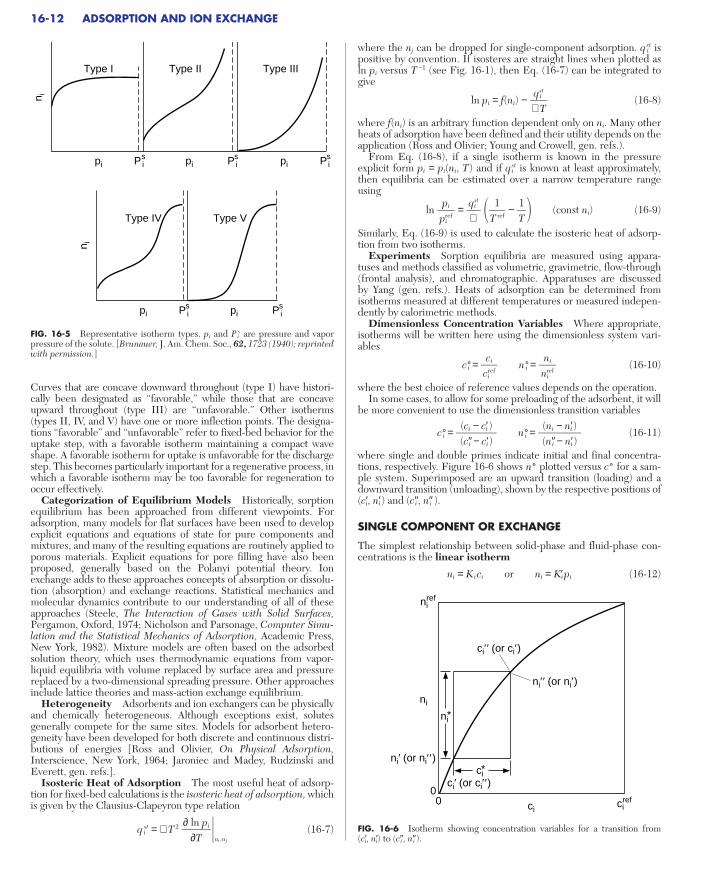
Curves that are concave downward throughout (type I) have histori-cally been designated as “favorable,” while those that are concaveupward throughout (type III) are “unfavorable.” Other isotherms(types II, IV, and V) have one or more inflection points. The designa-tions “favorable” and “unfavorable” refer to fixed-bed behavior for theuptake step, with a favorable isotherm maintaining a compact waveshape. A favorable isotherm for uptake is unfavorable for the dischargestep. This becomes particularly important for a regenerative process, inwhich a favorable isotherm may be too favorable for regeneration tooccur effectively.
Categorization of Equilibrium Models Historically, sorptionequilibrium has been approached from different viewpoints. Foradsorption, many models for flat surfaces have been used to developexplicit equations and equations of state for pure components andmixtures, and many of the resulting equations are routinely applied toporous materials. Explicit equations for pore filling have also beenproposed, generally based on the Polanyi potential theory. Ionexchange adds to these approaches concepts of absorption or dissolu-tion (absorption) and exchange reactions. Statistical mechanics andmolecular dynamics contribute to our understanding of all of theseapproaches (Steele, The Interaction of Gases with Solid Surfaces,Pergamon, Oxford, 1974; Nicholson and Parsonage, Computer Simu-lation and the Statistical Mechanics of Adsorption, Academic Press,New York, 1982). Mixture models are often based on the adsorbedsolution theory, which uses thermodynamic equations from vapor-liquid equilibria with volume replaced by surface area and pressurereplaced by a two-dimensional spreading pressure. Other approachesinclude lattice theories and mass-action exchange equilibrium.
Heterogeneity Adsorbents and ion exchangers can be physicallyand chemically heterogeneous. Although exceptions exist, solutesgenerally compete for the same sites. Models for adsorbent hetero-geneity have been developed for both discrete and continuous distri-butions of energies [Ross and Olivier, On Physical Adsorption,Interscience, New York, 1964; Jaroniec and Madey, Rudzinski andEverett, gen. refs.].
Isosteric Heat of Adsorption The most useful heat of adsorp-tion for fixed-bed calculations is the isosteric heat of adsorption, whichis given by the Clausius-Clapeyron type relation
qist = ℜ T 2
ni ,nj
(16-7)∂ ln pi
∂T
where the nj can be dropped for single-component adsorption. qist is
positive by convention. If isosteres are straight lines when plotted as ln pi versus T −1 (see Fig. 16-1), then Eq. (16-7) can be integrated togive
ln pi = f(ni) − (16-8)
where f(ni) is an arbitrary function dependent only on ni. Many otherheats of adsorption have been defined and their utility depends on theapplication (Ross and Olivier; Young and Crowell, gen. refs.).
From Eq. (16-8), if a single isotherm is known in the pressureexplicit form pi = pi(ni, T) and if qi
st is known at least approximately,then equilibria can be estimated over a narrow temperature rangeusing
ln = − (const ni) (16-9)
Similarly, Eq. (16-9) is used to calculate the isosteric heat of adsorp-tion from two isotherms.
Experiments Sorption equilibria are measured using appara-tuses and methods classified as volumetric, gravimetric, flow-through(frontal analysis), and chromatographic. Apparatuses are discussed by Yang (gen. refs.). Heats of adsorption can be determined fromisotherms measured at different temperatures or measured indepen-dently by calorimetric methods.
Dimensionless Concentration Variables Where appropriate,isotherms will be written here using the dimensionless system vari-ables
c*i = n*i = (16-10)
where the best choice of reference values depends on the operation.In some cases, to allow for some preloading of the adsorbent, it will
be more convenient to use the dimensionless transition variables
c*i = n*i = (16-11)
where single and double primes indicate initial and final concentra-tions, respectively. Figure 16-6 shows n* plotted versus c* for a sam-ple system. Superimposed are an upward transition (loading) and adownward transition (unloading), shown by the respective positions of(c′i, n′i ) and (c″i , n″i ).
SINGLE COMPONENT OR EXCHANGE
The simplest relationship between solid-phase and fluid-phase con-centrations is the linear isotherm
ni = Kici or ni = K′ipi (16-12)
(ni − n′i)(n″i − n′i )
(ci − c′i )(c″i − c′i)
nini
ref
cici
ref
1T
1T ref
qist
ℜ
pipi
ref
qist
ℜ T
16-12 ADSORPTION AND ION EXCHANGEn i
n i
P is P i
s Pispipipi
Type I Type II Type III
P is Pi
spipi
Type IV Type V
FIG. 16-5 Representative isotherm types. pi and Pis are pressure and vapor
pressure of the solute. [Brunauer, J. Am. Chem. Soc., 62, 1723 (1940); reprintedwith permission.]
00 ci
ref
niref
ni
ci*
ni′′ (or ni′)
ni*
ci′′ (or ci′)
ci′ (or ci′′ )
ci
ni′ (or ni′′ )
FIG. 16-6 Isotherm showing concentration variables for a transition from (c′i, n′i) to (c″i , n″i ).

Thermodynamics requires that a linear limit be approached in theHenry’s law region for all isotherm equations.
Flat Surface Isotherm Equations The classification of isothermequations into two broad categories for flat surfaces and pore fillingreflects their origin. It does not restrict equations developed for flatsurfaces from being applied successfully to describe data for porousadsorbents.
The classical isotherm for a homogeneous flat surface, and mostpopular of all nonlinear isotherms, is the Langmuir isotherm
ni = (16-13)
where nis is the monolayer capacity approached at large concentrations
and K i is an equilibrium constant. These parameters are often deter-mined by plotting 1/ni versus 1/ci. The derivation of the isothermassumes negligible interaction between adsorbed molecules.
The classical isotherm for multilayer adsorption on a homogeneous,flat surface is the BET isotherm [Brunauer, Emmett, and Teller, J. Am. Chem. Soc., 60, 309 (1938)]
ni = (16-14)
where pi is the pressure of the adsorbable component and Pis is its
vapor pressure. It is useful for gas-solid systems in which condensa-tion is approached, fitting type-II behavior.
For a heterogeneous flat surface, a classical isotherm is theFreundlich isotherm
ni = Kicimi (16-15)
where mi is positive and generally not an integer. The isotherm corre-sponds approximately to an exponential distribution of heats ofadsorption. Although it lacks the required linear behavior in theHenry’s law region, it can often be used to correlate data on heteroge-neous adsorbents over wide ranges of concentration.
Several isotherms combine aspects of both the Langmuir andFreudlich equations. One that has been shown to be effective indescribing data mathematically for heterogeneous adsorbents is theTóth isotherm [Acta Chim. Acad. Sci. Hung., 69, 311 (1971)]
ni = (16-16)
This three-parameter equation behaves linearly in the Henry’s lawregion and reduces to the Langmuir isotherm for m = 1. Other well-known isotherms include the Radke-Prausnitz isotherm [Radkeand Prausnitz, Ind. Eng. Chem. Fundam., 11, 445 (1972); AIChE J.,18, 761 (1972)]
ni = (16-17)
and the Sips isotherm [Sips, J. Chem. Phys., 16, 490 (1948); Kobleand Corrigan, Ind. Eng. Chem., 44, 383 (1952)] or loading ratio cor-relation with prescribed temperature dependence [Yon and Turnock,AIChE Symp. Ser., 67(117), 75 (1971)]
ni = (16-18)
Another three-parameter equation that often fits data well and islinear in the Henry’s law region is the UNILAN equation [Honig andReyerson, J. Phys. Chem., 56, 140 (1952)]
ni = ln (16-19)
which reduces to the Langmuir equation as si → 0.Equations of state are also used for pure components. Given such
an equation written in terms of the two-dimensional spreading pres-sure π, the corresponding isotherm is easily determined, as describedlater for mixtures [see Eq. (16-42)]. The two-dimensional equivalentof an ideal gas is an ideal surface gas, which is described by
πA = niℜ T (16-20)
which readily gives the linear isotherm, Eq. (16-12). Many more com-
1 + Kiesipi1 + Kie−sipi
nis
2si
nis(Kipi)m
1 + (Kipi)m
nisKipi
(1 + Kipi)m
nispi
[(1/Ki) + pi
mi]1/mi
nisKipi
[1 + Kipi − (pi /Pi
s)][1 − (pi /Pis)]
nisK ici
1 + Kici
plicated equations of state are available, including two-dimensionalanalogs of the virial equation and equations of van der Waals, Redlich-Kwong, Peng-Robinson, and so forth [Adamson, gen. refs.; Patry-kiejewet et al., Chem. Eng. J., 15, 147 (1978); Haydel and Kobayashi,Ind. Eng. Chem. Fundam., 6, 546 (1967)].
Pore-Filling Isotherm Equations Most pore-filling models aregrounded in the Polanyi potential theory. In Polanyi’s model, anattracting potential energy field is assumed to exist adjacent to the sur-face of the adsorbent and concentrates vapors there. Adsorption takesplace whenever the strength of the field, independent of temperature,is great enough to compress the solute to a partial pressure greaterthan its vapor pressure. The last molecules to adsorb form an equipo-tential surface containing the adsorbed volume. The strength of thisfield, called the adsorption potential ε (J/mol), was defined by Polanyito be equal to the work required to compress the solute from its par-tial pressure to its vapor pressure
ε = ℜ T ln (16-21)
The same result is obtained by considering the change in chemicalpotential. In the basic theory, W (m3/kg), the volume adsorbed as sat-urated liquid at the adsorption temperature, is plotted versus ε to givea characteristic curve. Data measured at different temperatures forthe same solute-adsorbent pair should fall on this curve. Using themethod, it is possible to use data measured at a single temperature topredict isotherms at other temperatures. Data for additional, homolo-gous solutes can be collapsed into a single “correlation curve” bydefining a scaling factor β, the most useful of which has been V/V ref,the adsorbate molar volume as saturated liquid at the adsorption tem-perature divided by that for a reference compound. Thus, by plottingW versus ε/β or ε/ V for data measured at various temperatures for var-ious similar solutes and a single adsorbent, a single curve should beobtained. Variations of the theory are often used to evaluate proper-ties for components near or above their critical points [Grant andManes, Ind. Eng. Chem. Fund., 5, 490 (1966)].
The most popular equations used to describe the shape of a charac-teristic curve or a correlation curve are the two-parameter Dubinin-Radushkevich (DR) equation
= exp−k 2
(16-22)
and the three-parameter Dubinin-Astakhov (DA) equation
= exp−k m
(16-23)
where W0 is micropore volume and m is related to the pore size distri-bution [Gregg and Sing, gen. refs.]. Neither of these equations hascorrect limiting behavior in the Henry’s law regime.
Ion Exchange A useful tool is provided by the mass action lawfor describing the general exchange equilibrium in fully ionizedexchanger systems as
zBA + zABA zBA + zAB
where overbars indicate the ionic species in the ion exchanger phaseand zA and zB are the valences of ions A and B. The associated equilib-rium relation is of the form
KcA,B = KA,B
zB zA
= zB
zA
(16-24)
where KcA,B is the apparent equilibrium constant or molar selectivity
coefficient, KA,B is the thermodynamic equilibrium constant based onactivities, and the γs are activity coefficients. Often it is desirable torepresent concentrations in terms of equivalent ionic fractions basedon solution normality ctot and fixed exchanger capacity ns as c*i = zici /ctot
and n*i = zini /ntot, where ctot = zjcj and ntot = zjnj = ns with the sum-mations extended to all counter-ion species. A rational selectivity coef-ficient is then defined as
K′A,B = KcA,B
zA − zB
= zB
zA
(16-25)
For the exchange of ions of equal valence (zA = zB), KcA,B and K′A,B are
c*Bn*B
n*Ac*A
ntotctot
cBnB
nAcA
γBγB
γAγA
εβ
WW0
εβ
WW0
Pis
pi
SORPTION EQUILIBRIUM 16-13

coincident and, to a first approximation, independent of concentra-tion. When zA > zB, K′A,B decreases with solution normality. Thisreflects the fact that ion exchangers exhibit an increasing affinity forions of lower valence as the solution normality increases.
An alternate form of Eq. (16-25) is
n*A = KcA,B
(zA − zB )/zB zA /zB
c*A (16-26)
When B is in excess (c*A, n*A → 0), this reduces to
n*A = KcA,B
(zA − zB )/zB
c*A = KAc*A (16-27)
where the linear equilibrium constant KA = KcA,B(ntot /ctot)(zA/zB) − 1
decreases with solution normality ctot when zA > zB or increases whenzA < zB.
Table 16-7 gives equilibrium constants for crosslinked cation andanion exchangers for a variety of counterions. The values given forcation exchangers are based on ion A replacing Li+, and those given foranion exchangers are based on ion A replacing Cl−. The selectivity for a particular ion generally increases with decreasing hydrated ionsize and increasing degree of crosslinking. The selectivity coefficientfor any two ions A and D can be obtained from Table 16-7 from valuesof KA,B and KD,B as
KA,D = KA,B /KD,B (16-28)
The values given in this table are only approximate, but they are ade-quate for process screening purposes with Eqs. (16-24) and (16-25).Rigorous calculations generally require that activity coefficients beaccounted for. However, for the exchange between ions of the samevalence at solution concentrations of 0.1 N or less, or between any ionsat 0.01 N or less, the solution-phase activity coefficients prorated tounit valence will be similar enough that they can be omitted.
Models for ion exchange equilibria based on the mass-action lawtaking into account solution and exchanger-phase nonidealities withequations similar to those for liquid mixtures have been developed byseveral authors [see Smith and Woodburn, AIChE J., 24, 577 (1978);Mehablia et al., Chem. Eng. Sci., 49, 2277 (1994)]. Thermodynamics-based approaches are also available [Soldatov in Dorfner, gen. refs.;Novosad and Myers, Can J. Chem. Eng., 60, 500 (1982); Myers andByington in Rodrigues, ed., Ion Exchange Science and Technology,NATO ASI Series, No. 107, Nijhoff, Dordrecht, 1986, pp. 119–145] as
ntotctot
1 − n*A1 − c*A
ntotctot
well as approaches for the exchange of macromolecules, taking intoaccount steric-hindrance effects [Brooks and Cramer, AIChE J., 38,12 (1992)].
Example 3: Calculation of Useful Ion-Exchange Capacity An8 percent crosslinked sulfonated resin is used to remove calcium from a solutioncontaining 0.0007 mol/l Ca+2 and 0.01 mol/l Na+. The resin capacity is 2.0equiv/l. Estimate the resin capacity for calcium removal.
From Table 16-7, we obtain KCa,Na = 5.16/1.98 = 2.6. Since ntot = 2 equiv/l andctot = 2 × 0.0007 + 0.01 = 0.024 equiv/l, K′Ca,Na = 2.6 × 2/0.011 = 470. Thus, withc*Ca = 2 × 0.0007/0.011 = 0.13, Eq. (16-25) gives 470 = (n*Ca /0.13)[(1 − 0.13)/(1 − n*Na)]2 or n*Ca = 0.9. The available capacity for calcium is nCa = 0.9 × 2.0/2 =0.9 mol/l.
Donnan Uptake The uptake of an electrolyte as a neutral ionpair of a salt is called Donnan uptake. It is generally negligible at lowionic concentrations. Above 0.5 g⋅equiv/l with strongly ionized ex-changers (or at lower concentrations with those more weakly ionized),the resin’s fixed ion-exchange capacity is measurably exceeded as aresult of electrolyte invasion. With only one coion species Y (matchingthe charge sign of the fixed groups in the resin), its uptake nY equalsthe total excess uptake of the counterion. Equilibrium is described bythe mass-action law. For the case of a resin in A-form in equilibriumwith a salt AY, the excess counterion uptake is given by [Helfferich,gen. refs., pp. 133–147]
zYnY = + (zYcY)2 2
AY / w
1/2
− (16-29)
where γs are activity coefficients, as water activities, and νs partialmolar volumes. For dilute conditions, Eq. (16-29) predicts a squareddependence of nY on cY. Thus, the electrolyte sorption isotherm has astrong positive curvature. Donnan uptake is more pronounced forresins of lower degree of crosslinking and for counterions of lowvalence.
Separation Factor By analogy with the mass-action case andappropriate for both adsorption and ion exchange, a separation fac-tor r can be defined based on dimensionless system variables [Eq.(16-10)] by
r = or r = (16-30)
This term is analogous to relative volatility or its reciprocal (or to anequilibrium selectivity). Similarly, the assumption of a constant sepa-
n*B /c*Bn*A /c*A
c*i (1 − n*i )n*i(1 − c*i )
ns
2
awaw
γAYγAY
ns2
4
16-14 ADSORPTION AND ION EXCHANGE
TABLE 16-7 Equilibrium Constants for Polystyrene DVB Cation and Anion Exchangers
Strong acid sulfonated cation exchangers (Li+ reference ion)
Degree of crosslinking Degree of crosslinking
Counter- 4% 8% 16% Counter- 4% 8% 16%ion DVB DVB DVB ion DVB DVB DVB
Li+ 1.00 1.00 1.00 Mg++ 2.95 3.29 3.51H+ 1.32 1.27 1.47 Zn++ 3.13 3.47 3.78Na+ 1.58 1.98 2.37 Co++ 3.23 3.74 3.81NH4
+ 1.90 2.55 3.34 Cu++ 3.29 3.85 4.46K+ 2.27 2.90 4.50 Cd++ 3.37 3.88 4.95Rb+ 2.46 3.16 4.62 Ni++ 3.45 3.93 4.06Cs+ 2.67 3.25 4.66 Ca++ 4.15 5.16 7.27Ag+ 4.73 8.51 22.9 Pb++ 6.56 9.91 18.0Tl+ 6.71 12.4 28.5 Ba++ 7.47 11.5 20.8
Strong base anion exchangers, 8% DVB (Cl− reference ion)
Type I Type II Type I Type IICounterion resin* resin† Counterion resin(a) resin(b)
Salicylate 32 28 Cyanide 1.6 1.3Iodide 8.7 7.3 Chloride 1.0 1.0Phenoxide 5.2 8.7 Hydroxide 0.05–0.07 0.65Nitrate 3.8 3.3 Bicarbonate 0.3 0.5Bromide 2.8 2.3 Formate 0.2 0.2Nitrite 1.2 1.3 Acetate 0.2 0.2Bisulfite 1.3 1.3 Fluoride 0.09 0.1Cyanide 1.6 1.3 Sulfate 0.15 0.15
*Trimethylamine†Dimethyl-hydroxyethylamineData from Bonner and Smith, J. Phys. Chem., 61, 326 (1957) and Wheaton and Bauman, Ind. Eng. Chem., 45, 1088 (1951).

ration factor is a useful assumption in many sorptive operations. [It isconstant for the Langmuir isotherm, as described below, and for mass-action equilibrium with m = 1 in Eq. (16-24).] This gives the constantseparation factor isotherm
n*i = (16-31)
The separation factor r identifies the equilibrium increase in n*i from0 to 1, which accompanies an increase in c*i from 0 to 1. For a concen-tration change over only part of the isotherm, a separation factor R can be defined for the dimensionless transition variables [Eq. (16-11)]. This separation factor is
R = = (16-32)
and gives an equation identical to Eq. (16-31) with R replacing r.Figure 16-7 shows constant separation factor isotherms for a range
of r (or R) values. The isotherm is linear for r = 1, favorable for r < 1,rectangular (or irreversible) for r = 0, and unfavorable for r > 1. As aresult of symmetry properties, if r is defined for adsorption of compo-nent i or exchange of ion A for B, then the reverse process is describedby 1/r.
The Langmuir isotherm, Eq. (16-13), corresponds to the constantseparation factor isotherm with
r = 1/(1 + Kic iref ) (16-33)
for system variables Eq. (16-10) or
R = (16-34)
for transition variables [Eq. (16-11)]. Vermeulen et al. [gen. refs.] giveadditional properties of constant separation factor isotherms.
Example 4: Application of Isotherms Thomas [Ann. N.Y. Acad.Sci., 49, 161 (1948)] provides the following Langmuir isotherm for the adsorp-tion of anthracene from cyclohexane onto alumina:
ni =
with ni in mol anthracene/kg alumina and ci in mol anthracene/l liquid.a. What are the values of Ki and ni
s according to Eq. (16-13)?
Ki = 375 l/mol
nis = = 0.0587 mol/kg
22Ki
22ci1 + 375ci
r + (1 − r)(c′i /ciref )
r + (1 − r)(c″i /ci
ref )
c*i (1 − n*i )n*i(1 − c*i )
n″i /c″in′i /c′i
c*ir + (1 − r)c*i
b. For a feed concentration of 8.11 × 10⁻⁴ mol/l, what is the value of r?
r = = 0.766 [from Eq. (16-33)]
c. If the alumina is presaturated with liquid containing 2.35 × 10⁻⁴ mol/l andthe feed concentration is 8.11 × 10⁻⁴ mol/l, what is the value of R?
R = 0.834 [from Eq. (16-32) or (16-34)]
MULTIPLE COMPONENTS OR EXCHANGES
When more than one adsorbed species or more than two ion-exchanged species interact in some manner, equilibrium becomesmore complicated. Usually, thermodynamics provides a sound basisfor prediction.
Adsorbed-Solution Theory The common thermodynamicapproach to multicomponent adsorption treats adsorption equilib-rium in a way analogous to fluid-fluid equilibrium. The theory has asits basis the Gibbs adsorption isotherm [Young and Crowell, gen.refs.], which is
Adπ =i
ni dµi (const T) (16-35)
where µ is chemical potential. For an ideal gas (dµ = ℜ Td ln pi), if it isassumed that an adsorbed solution is defined with a pure-componentstandard state (as is common for a liquid solution), then Eq. (16-35)can be integrated to give [Rudisill and LeVan, Chem. Eng. Sci., 47,1239 (1992)]
pi = γi xiP iref(T, π) (16-36)
where γi and xi are the adsorbed-phase activity coefficient and molefraction of component i and Pi
ref is the standard state, specified to beat the temperature and spreading pressure of the mixture.
Equation (16-36) with γi = 1 provides the basis for the idealadsorbed-solution theory [Myers and Prausnitz, AIChE J., 11, 121(1965)]. The spreading pressure for a pure component is determinedby integrating Eq. (16-35) for a pure component to obtain
= Piref
0dpi (16-37)
where ni is given by the pure-component isotherm. Also, since xi =1, Eq. (16-36) with γi = 1 gives (pi /Pi
ref ) = 1. With no area change onmixing for the ideal solution, the total number of moles adsorbed perunit weight of adsorbent is determined using a two-dimensional formof Amagat’s law:
= (16-38)
where ntot = ni and niref is given by the pure-component isotherm at
Piref. Adsorbed-phase concentrations are calculated using ni = xintot.
Generally, different values of π [or πA/(ℜ T)] must be tried until theone is found that satisfies Eqs. (16-37) and xi = 1.
Example 5: Application of Ideal Adsorbed-Solution TheoryConsider a binary adsorbed mixture for which each pure component obeys theLangmuir equation, Eq. (16-13). Let n1
s = 4 mol/kg, n2s = 3 mol/kg, K1p1 =
K2p2 = 1. Use the ideal adsorbed-solution theory to determine n1 and n2.Substituting the pure component Langmuir isotherm
ni =
into Eq. (16-37) and integrating gives
= nis ln(1 + KiP i
ref )
which can be solved explicitly for KiPiref. Values are guessed for πA/(ℜ T), values
of KiPiref are calculated from the equation above, and xi = Kipi /(KiPi
ref ) = 1 ischecked to see if it is satisfied. Trial and error gives πA/(ℜ T) = 3.8530 mol/kg, K1P1
ref = 1.6202, K2P2ref = 2.6123, and x1 = 0.61720. Evaluating the pure-
component isotherms at the reference pressures and using Eq. (16-38) gives ntot = 2.3475 mol/kg, and finally ni = xintot gives n1 = 1.4489 mol/kg and n2 =0.8986 mol/kg.
Other approaches to account for various effects have been devel-oped. Negative deviations from Raoult’s law (i.e., γi < 1) are frequently
πAℜ T
nisKipi
1 + Kipi
xini
ref
1ntot
nipi
πAℜ T
11 + Ki(8.11 × 10⁻⁴)
SORPTION EQUILIBRIUM 16-15
FIG. 16-7 Constant separation factor isotherm as a function of the separationfactor r (or interchangeably R). Each isotherm is symmetric about the perpen-dicular line connecting (0,1) and (1,0). Isotherms for r and 1/r are symmetricabout the 45° line.
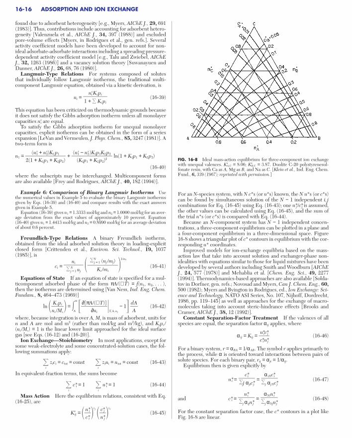
found due to adsorbent heterogeneity [e.g., Myers, AIChE J., 29, 691(1983)]. Thus, contributions include accounting for adsorbent hetero-geneity [Valenzuela et al., AIChE J., 34, 397 (1988)] and excludedpore-volume effects [Myers, in Rodrigues et al., gen. refs.]. Severalactivity coefficient models have been developed to account for non-ideal adsorbate-adsorbate interactions including a spreading pressure-dependent activity coefficient model [e.g., Talu and Zwiebel, AIChEJ., 32, 1263 (1986)] and a vacancy solution theory [Suwanayuen andDanner, AIChE J., 26, 68, 76 (1980)].
Langmuir-Type Relations For systems composed of solutesthat individually follow Langmuir isotherms, the traditional multi-component Langmuir equation, obtained via a kinetic derivation, is
ni = (16-39)
This equation has been criticized on thermodynamic grounds becauseit does not satisfy the Gibbs adsorption isotherm unless all monolayercapacities ns
i are equal.To satisfy the Gibbs adsorption isotherm for unequal monolayer
capacities, explicit isotherms can be obtained in the form of a seriesexpansion [LeVan and Vermeulen, J. Phys. Chem., 85, 3247 (1981)]. Atwo-term form is
n1 = + ln(1 + K1p1 + K2p2)
(16-40)
where the subscripts may be interchanged. Multicomponent formsare also available [Frey and Rodrigues, AIChE J., 40, 182 (1994)].
Example 6: Comparison of Binary Langmuir Isotherms Usethe numerical values in Example 5 to evaluate the binary Langmuir isothermsgiven by Eqs. (16-39) and (16-40) and compare results with the exact answersgiven in Example 5.
Equation (16-39) gives n1 = 1.3333 mol/kg and n2 = 1.0000 mol/kg for an aver-age deviation from the exact values of approximately 10 percent. Equation (16-40) gives n1 = 1.4413 mol/kg and n2 = 0.8990 mol/kg for an average deviationof about 0.6 percent.
Freundlich-Type Relations A binary Freundlich isotherm,obtained from the ideal adsorbed solution theory in loading-explicitclosed form [Crittenden et al., Environ. Sci. Technol., 19, 1037(1985)], is
ci = 1/mi
(16-41)
Equations of State If an equation of state is specified for a mul-ticomponent adsorbed phase of the form πA/(ℜ T) = f(n1, n2, . . . ),then the isotherms are determined using [Van Ness, Ind. Eng. Chem.Fundam., 8, 464–473 (1969)]
ln = ∞
A
T,A,nj
− 1 (16-42)
where, because integration is over A, Ms is mass of adsorbent, units forn and A are mol and m2 (rather than mol/kg and m2/kg), and Kipi /(ni /Ms) = 1 is the linear lower limit approached for the ideal surfacegas [see Eqs. (16-12) and (16-20)].
Ion Exchange—Stoichiometry In most applications, except forsome weak-electrolyte and some concentrated-solution cases, the fol-lowing summations apply:
i
zici = ctot = const i
zini = ntot = const (16-43)
In equivalent-fraction terms, the sums become
i
c*i = 1 i
n*i = 1 (16-44)
Mass Action Here the equilibrium relations, consistent with Eq.(16-25), are
K′ij = zj
zi
(16-45)c*jn*j
n*ic*i
dAA
∂[πA/(ℜ T)]
∂ni
Kipini /Ms
Nj = 1 (nj /mj)
Ki /mi
niN
j = 1 nj
(n1s − n2
s )K1p1K2p2
(K1p1 + K2p2)2
(n1s + n2
s)K1p12(1 + K1p1 + K2p2)
nisKipi
1 + Kipi
For an N-species system, with N c*s (or n*s) known, the N n*s (or c*s)can be found by simultaneous solution of the N − 1 independent i, jcombinations for Eq. (16-45) using Eq. (16-43); one n*j /c*j is assumed,the other values can be calculated using Eq. (16-45), and the sum ofthe trial n*s (or c*s) is compared with Eq. (16-44).
Because an N-component system has N − 1 independent concen-trations, a three-component equilibrium can be plotted in a plane anda four-component equilibrium in a three-dimensional space. Figure16-8 shows a triangular plot of c* contours in equilibrium with the cor-responding n* coordinates.
Improved models for ion-exchange equilibria based on the mass-action law that take into account solution and exchanger-phase non-idealities with equations similar to those for liquid mixtures have beendeveloped by several authors including Smith and Woodburn [AIChEJ., 24, 577 (1978)] and Mehablia et al. [Chem. Eng. Sci., 49, 2277(1994)]. Thermodynamics-based approaches are also available [Solda-tov in Dorfner, gen. refs.; Novosad and Myers, Can J. Chem. Eng., 60,500 (1982); Myers and Byington in Rodrigues, ed., Ion Exchange: Sci-ence and Technology, NATO ASI Series, No. 107, Nijhoff, Dordrecht,1986, pp. 119–145] as well as approaches for the exchange of macro-molecules taking into account steric-hindrance effects [Brooks andCramer, AIChE J., 38, 12 (1992)].
Constant Separation-Factor Treatment If the valences of allspecies are equal, the separation factor α ij applies, where
α ij = Kij = (16-46)
For a binary system, r = αBA = 1/αAB. The symbol r applies primarily tothe process, while α is oriented toward interactions between pairs ofsolute species. For each binary pair, rij = αji = 1/α ij.
Equilibrium then is given explicitly by
n*i = = (16-47)
and c*i = = (16-48)
For the constant separation factor case, the c* contours in a plot likeFig. 16-8 are linear.
αNin*ij αNjn*j
n*ij α ijn*j
α iNc*ij α jNc*j
c*ij α jic*j
n*ic*jc*in*j
16-16 ADSORPTION AND ION EXCHANGE
FIG. 16-8 Ideal mass-action equilibrium for three-component ion exchangewith unequal valences. K′A,C = 8.06; K′B,C = 3.87. Duolite C-20 polystyrenesul-fonate resin, with Ca as A, Mg as B, and Na as C. [Klein et al., Ind. Eng. Chem.Fund., 6, 339 (1967); reprinted with permission.]
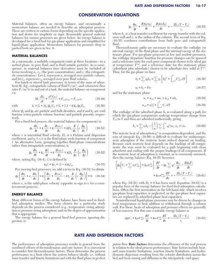
Material balances, often an energy balance, and occasionally amomentum balance are needed to describe an adsorption process.These are written in various forms depending on the specific applica-tion and desire for simplicity or rigor. Reasonably general materialbalances for various processes are given below. An energy balance isdeveloped for a fixed bed for gas-phase application and simplified forliquid-phase application. Momentum balances for pressure drop inpacked beds are given in Sec. 6.
MATERIAL BALANCES
At a microscale, a sorbable component exists at three locations—in asorbed phase, in pore fluid, and in fluid outside particles. As a conse-quence, in material balances time derivatives must be included ofterms involving ni, cpi (the pore concentration), and ci (the extraparti-cle concentration). Let ni represent ni averaged over particle volume,and let cpi represent cpi averaged over pore fluid volume.
For batch or stirred tank processes, in terms of the mass of adsor-bent Ms (kg), extraparticle volume of fluid Vf (m3), and volumetric flowrates Fv (m3/s) in and out of a tank, the material balance on componenti is
Ms + = Fv,incin,i − Fv,out ci (16-49)
with ni = ni + (εp /ρp)cpi = ni + [(1 − ε)εp /ρb]cpi (16-50)
where ρp and ρb are particle and bulk densities, and ε and εp are voidfraction (extra particle volume fraction) and particle porosity, respec-tively.
For a fixed-bed process, the material balance for component i is
ρb + ε + ε = εDL c (16-51)
where v is interstitial fluid velocity, DL is a Fickian axial dispersioncoefficient, and yi = ci /c is the fluid-phase mole fraction of componenti. An alternative form, grouping together fluid-phase concentrationsrather than intraparticle concentrations, is
ρb + εb + ε = εDL c (16-52)
where, noting Eq. (16-4), ci is defined byεbci = εci + (1 − ε)εpcpi (16-53)
For moving-bed processes, we add a term to Eq. (16-51) to obtain
ρb + vs + ε + − DL c = 0 (16-54)
where vs is the solid-phase velocity (opposite in sign to v for a coun-tercurrent process).
ENERGY BALANCE
Many different forms of the energy balance have been used in fixed-bed adsorption studies. The form chosen for a particular studydepends on the process considered (e.g., temperature swing adsorp-tion or pressure swing adsorption) and on the degree of approximationthat is appropriate.
The energy balance for a general fixed-bed process, ignoring dis-persion, is
∂yi∂z
∂∂z
∂(vci)
∂z∂ci∂t
∂ni∂z
∂ni∂t
∂yi∂z
∂∂z
∂(vci)
∂z∂ci∂t
∂ni∂t
∂yi∂z
∂∂z
∂(vci)
∂z∂ci∂t
∂ni∂t
d(Vfci)
dtdnidt
ρb + + = − (16-55)
where hw is a heat transfer coefficient for energy transfer with the col-umn wall and rc is the radius of the column. The second term of Eq.(16-55) combines contributions from both pore and extraparticlefluid.
Thermodynamic paths are necessary to evaluate the enthalpy (orinternal energy) of the fluid phase and the internal energy of the sta-tionary phase. For gas-phase processes at low and modest pressures,the enthalpy departure function for pressure changes can be ignoredand a reference state for each pure component chosen to be ideal gasat temperature T ref, and a reference state for the stationary phase(adsorbent plus adsorbate) chosen to be adsorbate-free solid at T ref.Thus, for the gas phase we have
hf = i
yihfi = i
yi hfiref + T
TrefC°pfi dT (16-56)
uf = hf − P/c (16-57)
and for the stationary phase
us = usol + nua ≈ usol + nha (16-58)
usol = usolref + T
TrefCs dT (16-59)
The enthalpy of the adsorbed phase ha is evaluated along a path forwhich the gas-phase components undergo temperature change fromTref to T and then are adsorbed isothermally, giving
ha = i
xihfi − i
ni
0qi
st(ni, nj, T) dni (16-60)
The isoteric heat of adsorption qist is composition-dependent, and the
sum of integrals Eq. (16-60) is difficult to evaluate for multicompo-nent adsorption if the isosteric heats indeed depend on loading.Because each isosteric heat depends on the loadings of all compo-nents, the sum must be evaluated for a path beginning with cleanadsorbent and ending with the proper loadings of all components. Ifthe isosteric heat of adsorption is constant, as is commonly assumed,then the energy balance (Eq. 16-55) becomes
ρbCs + i
niC°pfi + εbcC°pf − ρb i
qist −
+ εvcC°pf = − (16-61)
where Eq. (16-51) with DL = 0 has been used. Equation (16-61) is apopular form of the energy balance for fixed-bed adsorption calcula-tions. Often the first summation on the left-hand side, which involvesgas-phase heat capacities, is neglected, or the gas-phase heat capaci-ties are replaced by adsorbed-phase heat capacities.
Nonisothermal liquid-phase processes may be driven by changes infeed temperature or heat addition or withdrawal through a columnwall. For these, heats of adsorption and pressure effects are generallyof less concern. For this case a suitable energy balance is
(ρbCs + εbcC°pf) + εvcC°pf = − (16-62)2hw(T − Tw)
rc
∂T∂z
∂T∂t
2hw(T − Tw)
rc
∂T∂z
∂(εbP)
∂t∂ni∂t
∂T∂t
1n
2hw(T − Tw)
rc
∂(εvchf)
∂z
∂(εbcuf)
∂t∂us∂t
RATE AND DISPERSION FACTORS 16-17
CONSERVATION EQUATIONS
The performance of adsorption processes results in general from thecombined effects of thermodynamic and rate factors. It is convenientto consider first thermodynamic factors. These determine the processperformance in a limit where the system behaves ideally; i.e. withoutmass transfer and kinetic limitations and with the fluid phase in perfect
piston flow. Rate factors determine the efficiency of the real processin relation to the ideal process performance. Rate factors include heat-and mass-transfer limitations, reaction kinetic limitations, and hydro-dynamic dispersion resulting from the velocity distribution across thebed and from mixing and diffusion in the interparticle void space.
RATE AND DISPERSION FACTORS

TRANSPORT AND DISPERSION MECHANISMS
Figure 16-9 depicts porous adsorbent particles in an adsorption bedwith sufficient generality to illustrate the nature and location of indi-vidual transport and dispersion mechanisms. Each mechanism involvesa different driving force and, in general, gives rise to a different form ofmathematical result.
Intraparticle Transport Mechanisms Intraparticle transportmay be limited by pore diffusion, solid diffusion, reaction kinetics atphase boundaries, or two or more of these mechanisms together.
1. Pore diffusion in fluid-filled pores. These pores are suffi-ciently large that the adsorbing molecule escapes the force field of theadsorbent surface. Thus, this process is often referred to as macroporediffusion. The driving force for such a diffusion process can be approx-imated by the gradient in mole fraction or, if the molar concentrationis constant, by the gradient in concentration of the diffusing specieswithin the pores.
2. Solid diffusion in the adsorbed phase. Diffusion in pores suf-ficiently small that the diffusing molecule never escapes the forcefield of the adsorbent surface. In this case, transport may occur by anactivated process involving jumps between adsorption sites. Such aprocess is often called surface diffusion or, in the case of zeolites,micropore or intracrystalline diffusion. The driving force for theprocess can thus be approximated by the gradient in concentration ofthe species in its adsorbed state. Phenomenologically, the process isnot distinguishable from that of homogeneous diffusion that occursinside a sorbent gel or in a pore-filling fluid that is immiscible with theexternal fluid. The generic term solid diffusion is used here to encom-pass the general traits of these physically different systems.
3. Reaction kinetics at phase boundaries. Rates of adsorptionand desorption in porous adsorbents are generally controlled by masstransfer within the pore network rather than by the kinetics of sorp-tion at the surface. Exceptions are the cases of chemisorption andaffinity-adsorption systems used for biological separations, where thekinetics of bond formation can be exceedingly slow.
Intraparticle convection can also occur in packed beds when theadsorbent particles have very large and well-connected pores.Although, in general, bulk flow through the pores of the adsorbentparticles is only a small fraction of the total flow, intraparticle convec-tion can affect the transport of very slowly diffusing species such asmacromolecules. The driving force for convection, in this case, is the
pressure drop across each particle that is generated by the frictionalresistance to flow experienced by the fluid as this flows through thepacked bed [Rodrigues et al., Chem. Eng. Sci., 46, 2765 (1991); Cartaet al., Sep. Technol., 2, 62 (1992); Frey et al., Biotechnol. Progr., 9, 273(1993); Liapis and McCoy, J. Chromatogr., 599, 87 (1992)]. Intra-particle convection can also be significant when there is a total pres-sure difference between the center of the particle and the outside,such as is experienced in pressurization and depressurization steps ofpressure swing adsorption or when more gas is drawn into an adsor-bent to equalize pressure as adsorption occurs from the gas phasewithin a porous particle [Lu et al., AIChE J., 38, 857 (1992); Lu et al.,Gas Sep. Purif., 6, 89 (1992)].
Extraparticle Transport and Dispersion Mechanisms Extra-particle mechanisms are affected by the design of the contacting deviceand depend on the hydrodynamic conditions outside the particles.
4. External mass transfer between the external surfaces of theadsorbent particles and the surrounding fluid phase. The driving forceis the concentration difference across the boundary layer that sur-rounds each particle, and the latter is affected by the hydrodynamicconditions outside the particles.
5. Mixing, or lack of mixing, between different parts of the con-tacting equipment. This may occur through the existence of a velocitydistribution or dead zones in a packed bed or through inefficient mix-ing in an agitated contactor. In packed-bed adsorbers, mixing is oftendescribed in terms of an axial dispersion coefficient whereby all mech-anisms contributing to axial mixing are lumped together in a singleeffective coefficient.
Heat Transfer Since adsorption is generally accompanied by theevolution of heat, the rate of heat transfer between the adsorbent par-ticles and the fluid phase may be important. In addition, heat transfercan occur across the column wall in small diameter beds and is impor-tant in energy applications of adsorption. In gas adsorption systems,even with highly porous particles, the controlling heat transfer resis-tance is generally associated with extraparticle transport [Lee andRuthven, Can. J. Chem. Eng., 57, 65 (1979)], so that the temperaturewithin the particles is essentially uniform. In liquid-phase adsorption,intraparticle and extraparticle heat transfer resistances are generallycomparable. However, in this case the heat capacity of the fluid phaseis sufficiently high that temperature effects may be negligible exceptin extreme cases. General discussions of heat-transfer effects in adsor-bents and adsorption beds are found in Suzuki (gen. refs., pp. 187–208and pp. 275–290) and in Ruthven (gen. refs., pp. 189–198 and pp.215–219).
INTRAPARTICLE MASS TRANSFER
The phenomenological aspects of diffusional mass transfer in adsorp-tion systems can be described in terms of Fick’s law:
Ji = −Di(ci) (16-63)
This expression can be used to describe both pore and solid diffusionso long as the driving force is expressed in terms of the appropriateconcentrations. Although the driving force should be more correctlyexpressed in terms of chemical potentials, Eq. (16-63) provides a qual-itatively and quantitatively correct representation of adsorption sys-tems so long as the diffusivity is allowed to be a function of theadsorbate concentration. The diffusivity will be constant only for athermodynamically ideal system, which is only an adequate approxi-mation for a limited number of adsorption systems.
Results for several individual mechanisms will now be considered.The equations that follow refer to local conditions within the contact-ing equipment that may apply to the average concentrations in theneighborhood of a single adsorbent particle. Generally, they apply toparticles that can be approximated as spherical and of a uniform sizeand properties. An appropriately chosen mean particle size must beused in these equations when dealing with adsorbents having a broadparticle size distribution. The appropriate average depends on thecontrolling mass-transfer mechanism. For intraparticle mass-transfermechanisms, the volume or mass-average particle size usually pro-vides the best prediction.
∂ci∂x
16-18 ADSORPTION AND ION EXCHANGE
Flow
5 5
Wall
1 32
4
FIG. 16-9 General scheme of adsorbent particles in a packed bed showing thelocations of mass transfer and dispersive mechanisms. Numerals correspond tonumbered paragraphs in the text: 1, pore diffusion; 2, solid diffusion; 3, reactionkinetics at phase boundary; 4, external mass transfer; 5, fluid mixing.
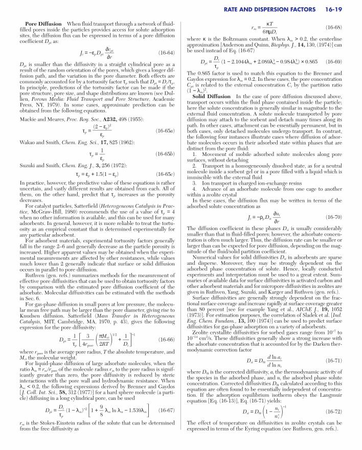
Pore Diffusion When fluid transport through a network of fluid-filled pores inside the particles provides access for solute adsorptionsites, the diffusion flux can be expressed in terms of a pore diffusioncoefficient Dpi as:
Ji = −εpDpi (16-64)
Dpi is smaller than the diffusivity in a straight cylindrical pore as aresult of the random orientation of the pores, which gives a longer dif-fusion path, and the variation in the pore diameter. Both effects arecommonly accounted for by a tortuosity factor τp such that Dpi = Di /τp.In principle, predictions of the tortuosity factor can be made if thepore structure, pore size, and shape distributions are known (see Dul-lien, Porous Media: Fluid Transport and Pore Structure, AcademicPress, NY, 1979). In some cases, approximate prediction can beobtained from the following equations.
Mackie and Meares, Proc. Roy. Soc., A232, 498 (1955):
τp = (16-65a)
Wakao and Smith, Chem. Eng. Sci., 17, 825 (1962):
τp = (16-65b)
Suzuki and Smith, Chem. Eng. J., 3, 256 (1972):
τp = εp + 1.5(1 − εp) (16-65c)
In practice, however, the predictive value of these equations is ratheruncertain, and vastly different results are obtained from each. All ofthem, on the other hand, predict that τp increases as the porositydecreases.
For catalyst particles, Satterfield (Heterogeneous Catalysis in Prac-tice, McGraw-Hill, 1980) recommends the use of a value of τp = 4when no other information is available, and this can be used for manyadsorbents. In general, however, it is more reliable to treat the tortu-osity as an empirical constant that is determined experimentally forany particular adsorbent.
For adsorbent materials, experimental tortuosity factors generallyfall in the range 2–6 and generally decrease as the particle porosity isincreased. Higher apparent values may be obtained when the experi-mental measurements are affected by other resistances, while valuesmuch lower than 2 generally indicate that surface or solid diffusionoccurs in parallel to pore diffusion.
Ruthven (gen. refs.) summarizes methods for the measurement ofeffective pore diffusivities that can be used to obtain tortuosity factorsby comparison with the estimated pore diffusion coefficient of theadsorbate. Molecular diffusivities can be estimated with the methodsin Sec. 6.
For gas-phase diffusion in small pores at low pressure, the molecu-lar mean free path may be larger than the pore diameter, giving rise toKnudsen diffusion. Satterfield (Mass Transfer in HeterogeneousCatalysis, MIT, Cambridge, MA, 1970, p. 43), gives the followingexpression for the pore diffusivity:
Dpi = 1/2
+ −1
(16-66)
where rpore is the average pore radius, T the absolute temperature, andMri the molecular weight.
For liquid-phase diffusion of large adsorbate molecules, when theratio λm = rm /rpore of the molecule radius rm to the pore radius is signif-icantly greater than zero, the pore diffusivity is reduced by stericinteractions with the pore wall and hydrodynamic resistance. Whenλm < 0.2, the following expressions derived by Brenner and Gaydos [J. Coll. Int. Sci., 58, 312 (1977)] for a hard sphere molecule (a parti-cle) diffusing in a long cylindrical pore, can be used
Dpi = (1 − λm)−2 1 + λm ln λm − 1.539λm (16-67)
rm is the Stokes-Einstein radius of the solute that can be determinedfrom the free diffusivity as
98
Diτp
1Di
πMri2RT
34rpore
1τp
1εp
(2 − εp)2
εp
∂cpi∂r
rm = (16-68)
where κ is the Boltzmann constant. When λm > 0.2, the centerlineapproximation [Anderson and Quinn, Biophys. J., 14, 130, (1974)] canbe used instead of Eq. (16-67)
Dpi = (1 − 2.1044λm + 2.089λm3 − 0.984λm
5 ) × 0.865 (16-69)
The 0.865 factor is used to match this equation to the Brenner andGaydos expression for λm = 0.2. In these cases, the pore concentrationCpi is related to the external concentration Ci by the partition ratio (1 − λm)2.
Solid Diffusion In the case of pore diffusion discussed above,transport occurs within the fluid phase contained inside the particle;here the solute concentration is generally similar in magnitude to theexternal fluid concentration. A solute molecule transported by porediffusion may attach to the sorbent and detach many times along itspath. In other cases, attachment can be essentially permanent, but inboth cases, only detached molecules undergo transport. In contrast,the following four instances illustrate cases where diffusion of adsor-bate molecules occurs in their adsorbed state within phases that aredistinct from the pore fluid:
1. Movement of mobile adsorbed solute molecules along poresurfaces, without detaching
2. Transport in a homogeneously dissolved state, as for a neutralmolecule inside a sorbent gel or in a pore filled with a liquid which isimmiscible with the external fluid
3. Ion transport in charged ion-exchange resins4. Advance of an adsorbate molecule from one cage to another
within a zeolite crystalIn these cases, the diffusion flux may be written in terms of the
adsorbed solute concentration as
Ji = −ρpDsi (16-70)
The diffusion coefficient in these phases Dsi is usually considerablysmaller than that in fluid-filled pores; however, the adsorbate concen-tration is often much larger. Thus, the diffusion rate can be smaller orlarger than can be expected for pore diffusion, depending on the mag-nitude of the fluid/solid partition coefficient.
Numerical values for solid diffusivities Dsi in adsorbents are sparseand disperse. Moreover, they may be strongly dependent on theadsorbed phase concentration of solute. Hence, locally conductedexperiments and interpretation must be used to a great extent. Sum-maries of available data for surface diffusivities in activated carbon andother adsorbent materials and for micropore diffusivities in zeolites aregiven in Ruthven, Yang, Suzuki, and Karger and Ruthven (gen. refs.).
Surface diffusivities are generally strongly dependent on the frac-tional surface coverage and increase rapidly at surface coverage greaterthan 80 percent [see for example Yang et al., AIChE J., 19, 1052(1973)]. For estimation purposes, the correlation of Sladek et al. [Ind.Eng. Chem. Fundam., 13, 100 (1974)] can be used to predict surfacediffusivities for gas-phase adsorption on a variety of adsorbents.
Zeolite crystallite diffusivities for sorbed gases range from 10−7 to10−14 cm2/s. These diffusivities generally show a strong increase withthe adsorbate concentration that is accounted for by the Darken ther-modynamic correction factor
Dsi = D0i (16-71)
where D0i is the corrected diffusivity, ai the thermodynamic activity ofthe species in the adsorbed phase, and ni the adsorbed phase soluteconcentration. Corrected diffusivities D0i calculated according to thisequation are often found to be essentially independent of concentra-tion. If the adsorption equilibrium isotherm obeys the Langmuirequation [Eq. (16-13)], Eq. (16-71) yields:
Dsi = D0i 1 − −1
(16-72)
The effect of temperature on diffusivities in zeolite crystals can beexpressed in terms of the Eyring equation (see Ruthven, gen. refs.).
nini
s
d ln aid ln ni
∂ni∂r
Diτp
κT6πµDi
RATE AND DISPERSION FACTORS 16-19

In ion-exchange resins, diffusion is further complicated by electri-cal coupling effects. In a system with M counterions, diffusion ratesare described by the Nernst-Planck equations (Helfferich, gen. refs.).Assuming complete Donnan exclusion, these equations can be writtenas:
Ji = −ρp z1
i
M − 1
j = 1
Di, j (16-73)
with Di, j = − (16-74a)
Di,i = Di − (16-74b)
which are dependent on the ionic self diffusivities Di of the individ-ual species. As a qualitative rule, ionic diffusivities of inorganic speciesin crosslinked polystyrene-DVB ion-exchange resins compared withthose in water are 1:10 for monovalent ions, 1:100 for divalent ions,and 1:1000 for trivalent ions. Table 16-8 shows typical ionic diffusivi-ties of inorganic ions in cation and anion exchange resins; largerorganic ions, however, can have ionic diffusivities much smaller thaninorganic ions of the same valence [see, for example, Jones and Carta,Ind. Eng. Chem. Research, 32, 117 (1993)].
For mixtures of unlike ions (the usual case), the apparent diffusivitywill be intermediate between these values because of the electricalcoupling effect. For a system with two counterions A and B, withcharge zA and zB, Eqs. (16-73) and (16-74) reduce to:
JA = −ρpDA, B = −ρp (16-75)
which shows that the apparent diffusivity DA,B varies between DA when the ionic fraction of species A in the resin is very small and DB when the ionic fraction of A in the resin approaches unity, indi-cating that the ion present in smaller concentration has the strongereffect on the local interdiffusion rate.
Combined Pore and Solid Diffusion In porous adsorbents andion-exchange resins, intraparticle transport can occur with pore andsolid diffusion in parallel. The dominant transport process is the fasterone, and this depends on the relative diffusivities and concentrationsin the pore fluid and in the adsorbed phase. Often, equilibriumbetween the pore fluid and the solid phase can be assumed to existlocally at each point within a particle. In this case, the mass-transferflux is expressed by:
Ji = −εpDpi + ρpDsi = −Dei(cpi) (16-76)
where dnie /dci is the derivative of the adsorption isotherm and it has
been assumed that at equilibrium cpi = ci. This equation suggests that
∂cpi∂r
∂cpi∂r
dnie
dci
∂nA∂r
DADB[zA2nA + zB
2nB]zA
2DAnA + zB2 DBnB
∂nA∂r
Di(Di − DM)z i2 ni
M
k = 1 Dkzk2 nk
Di(Dj − DM)z i2ni
M
k = 1 Dkzk2 nk
∂zjnj∂r
in such an adsorbent, pore and solid diffusivities can be obtained bydetermining the apparent diffusivity Dei for conditions of no adsorp-tion (dni
e /dci = 0) and for conditions of strong adsorption, wheredni
e /dci is large. If the adsorption isotherm is linear over the range ofexperimental measurement:
Dei = εp Dpi + ρpKiDsi (16-77)
Thus, a plot of the apparent diffusivity versus the linear adsorptionequilibrium constant should be linear so long as Dpi and Dsi remainconstant.
In a particle having a bidispersed pore structure comprisingspherical adsorptive subparticles of radius rs forming a macroporousaggregate, separate flux equations can be written for the macroporousnetwork in terms of Eq. (16-64) and for the subparticles themselves interms of Eq. (16-70) if solid diffusion occurs.
EXTERNAL MASS TRANSFER
Because of the complexities encountered with a rigorous treatment ofthe hydrodynamics around particles in industrial contactors, masstransfer to and from the adsorbent is described in terms of a mass-transfer coefficient kf. The flux at the particle surface is:
Ni = kf (ci − cis) (16-78)
where ci and cis are the solute concentrations in the bulk fluid and at
the particle surface, respectively. kf can be estimated from availablecorrelations in terms of the Sherwood number Sh = kf dp /Di and theSchmidt number Sc = ν/Di. For packed-bed operations, the correla-tions in Table 16-9 are recommended. A plot of these equations isgiven in Fig. 16-10 for representative ranges of Re and Sc with ε = 0.4.
External mass-transfer coefficients for particles suspended in agi-tated contactors can be estimated from equations in Levins and Glas-tonbury [Trans. Instn. Chem. Eng., 50, 132 (1972)] and Armenanteand Kirwan [Chem. Eng. Sci., 44, 2871 (1989)].
AXIAL DISPERSION IN PACKED BEDS
The axial dispersion coefficient [cf. Eq. (16-51)] lumps together allmechanisms leading to axial mixing in packed beds. Thus, the axialdispersion coefficient must account not only for molecular diffusionand convective mixing but also for nonuniformities in the fluid veloc-ity across the packed bed. As such, the axial dispersion coefficient isbest determined experimentally for each specific contactor.
The effects of flow nonuniformities, in particular, can be severein gas systems when the ratio of bed-to-particle diameters is small; inliquid systems when viscous fingering occurs as a result of large viscosity gradients in the adsorption bed; when very small particles(<50 µm) are used, such as in high performance liquid chromatog-raphy systems; and in large-diameter beds. A lower bound of the axial
16-20 ADSORPTION AND ION EXCHANGE
TABLE 16-8 Self Diffusion Coefficients in Polystyrene-divinylbenzene Ion Exchangers (units of 10-7 cm2/s)*
Temperature 0.3 °C 25 °C
Crosslinking, % 4 6 8 12 16 4 6 8 12 16
Cation exchangers (sulfonated): Dowex 50
Na+ 6.7 3.4 1.15 0.66 14.1 9.44 2.40Cs+ 6.6 1.11 13.7 3.10Ag+ 2.62 1.00 6.42 2.75Zn2+ 0.21 0.03 0.63 0.14La3+ 0.30 0.03 0.002 0.092 0.005
Anion exchangers (dimethyl hydroxyethylamine): Dowex 2
Cl− 1.25 3.54Br− (1.8) 1.50 0.63 0.06 (4.3) 3.87 2.04 0.26I− 0.35 1.33BrO3
− 1.76 4.55WO4
2− 0.60 1.80PO4
3− 0.16 0.57
*Data from Boyd and Soldano, J. Am. Chem. Soc., 75, 6091 (1953).
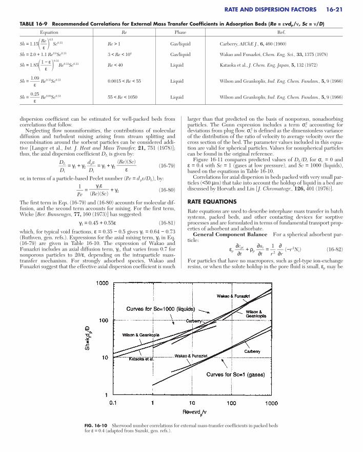
dispersion coefficient can be estimated for well-packed beds fromcorrelations that follow.
Neglecting flow nonuniformities, the contributions of moleculardiffusion and turbulent mixing arising from stream splitting andrecombination around the sorbent particles can be considered addi-tive [Langer et al., Int. J. Heat and Mass Transfer, 21, 751 (1978)];thus, the axial dispersion coefficient DL is given by:
= γ1 + γ2 = γ1 + γ2 (16-79)
or, in terms of a particle-based Peclet number (Pe = dpv/DL), by:
= + γ2 (16-80)
The first term in Eqs. (16-79) and (16-80) accounts for molecular dif-fusion, and the second term accounts for mixing. For the first term,Wicke [Ber. Bunsenges, 77, 160 (1973)] has suggested:
γ1 = 0.45 + 0.55ε (16-81)
which, for typical void fractions, ε = 0.35 − 0.5 gives γ1 = 0.64 − 0.73(Ruthven, gen. refs.). Expressions for the axial mixing term, γ2 in Eq.(16-79) are given in Table 16-10. The expression of Wakao andFunazkri includes an axial diffusion term, γ1, that varies from 0.7 fornonporous particles to 20/ε, depending on the intraparticle mass-transfer mechanism. For strongly adsorbed species, Wakao andFunazkri suggest that the effective axial dispersion coefficient is much
γ1ε(Re)(Sc)
1Pe
(Re)(Sc)
εdpvDi
DLDi
larger than that predicted on the basis of nonporous, nonadsorbingparticles. The Gunn expression includes a term σv
2 accounting fordeviations from plug flow. σv
2 is defined as the dimensionless varianceof the distribution of the ratio of velocity to average velocity over thecross section of the bed. The parameter values included in this equa-tion are valid for spherical particles. Values for nonspherical particlescan be found in the original reference.
Figure 16-11 compares predicted values of DL /Di for σv = 0 and ε = 0.4 with Sc = 1 (gases at low pressure), and Sc = 1000 (liquids),based on the equations in Table 16-10.
Correlations for axial dispersion in beds packed with very small par-ticles (<50 µm) that take into account the holdup of liquid in a bed arediscussed by Horvath and Lin [J. Chromatogr., 126, 401 (1976)].
RATE EQUATIONS
Rate equations are used to describe interphase mass transfer in batchsystems, packed beds, and other contacting devices for sorptiveprocesses and are formulated in terms of fundamental transport prop-erties of adsorbent and adsorbate.
General Component Balance For a spherical adsorbent par-ticle:
εp + ρp = (−r 2Ni) (16-82)
For particles that have no macropores, such as gel-type ion-exchangeresins, or when the solute holdup in the pore fluid is small, εp may be
∂∂r
1r 2
∂ni∂t
∂cpi∂t
RATE AND DISPERSION FACTORS 16-21
TABLE 16-9 Recommended Correlations for External Mass Transfer Coefficients in Adsorption Beds (Re = evdp/n, Sc = n/D)
Equation Re Phase Ref.
Sh = 1.15 0.5
Sc0.33 Re > 1 Gas/liquid Carberry, AIChE J., 6, 460 (1960)
Sh = 2.0 + 1.1 Re0.6Sc0.33 3 < Re < 104 Gas/liquid Wakao and Funazkri, Chem. Eng. Sci., 33, 1375 (1978)
Sh = 1.85 0.33
Re0.33Sc0.33 Re < 40 Liquid Kataoka et al., J. Chem. Eng. Japan, 5, 132 (1972)
Sh = Re0.33Sc0.33 0.0015 < Re < 55 Liquid Wilson and Geankoplis, Ind. Eng. Chem. Fundam., 5, 9 (1966)
Sh = Re0.69Sc0.33 55 < Re < 1050 Liquid Wilson and Geankoplis, Ind. Eng. Chem. Fundam., 5, 9 (1966)0.25
ε
1.09
ε
1 − ε
ε
Reε
FIG. 16-10 Sherwood number correlations for external mass-transfer coefficients in packed bedsfor ε = 0.4 (adapted from Suzuki, gen. refs.).
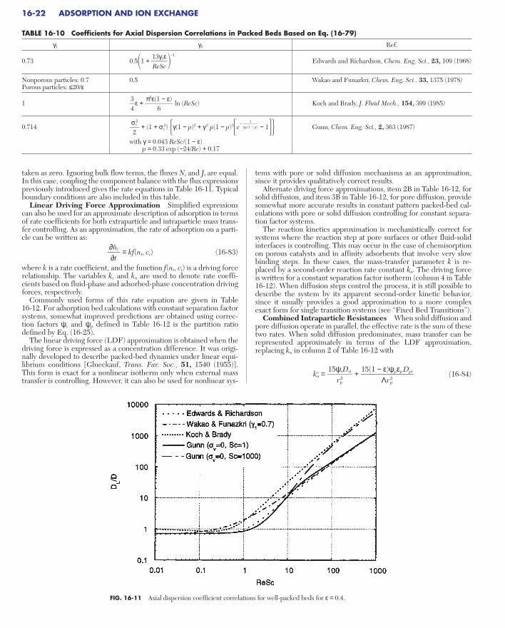
taken as zero. Ignoring bulk flow terms, the fluxes Ni and Ji are equal.In this case, coupling the component balance with the flux expressionspreviously introduced gives the rate equations in Table 16-11. Typicalboundary conditions are also included in this table.
Linear Driving Force Approximation Simplified expressionscan also be used for an approximate description of adsorption in termsof rate coefficients for both extraparticle and intraparticle mass trans-fer controlling. As an approximation, the rate of adsorption on a parti-cle can be written as:
= kf(ni, ci) (16-83)
where k is a rate coefficient, and the function f(ni, ci) is a driving forcerelationship. The variables kc and kn are used to denote rate coeffi-cients based on fluid-phase and adsorbed-phase concentration drivingforces, respectively.
Commonly used forms of this rate equation are given in Table 16-12. For adsorption bed calculations with constant separation factorsystems, somewhat improved predictions are obtained using correc-tion factors ψs and ψp defined in Table 16-12 is the partition ratiodefined by Eq. (16-25).
The linear driving force (LDF) approximation is obtained when thedriving force is expressed as a concentration difference. It was origi-nally developed to describe packed-bed dynamics under linear equi-librium conditions [Glueckauf, Trans. Far. Soc., 51, 1540 (1955)].This form is exact for a nonlinear isotherm only when external masstransfer is controlling. However, it can also be used for nonlinear sys-
∂ni∂t
tems with pore or solid diffusion mechanisms as an approximation,since it provides qualitatively correct results.
Alternate driving force approximations, item 2B in Table 16-12, forsolid diffusion, and item 3B in Table 16-12, for pore diffusion, providesomewhat more accurate results in constant pattern packed-bed cal-culations with pore or solid diffusion controlling for constant separa-tion factor systems.
The reaction kinetics approximation is mechanistically correct forsystems where the reaction step at pore surfaces or other fluid-solidinterfaces is controlling. This may occur in the case of chemisorptionon porous catalysts and in affinity adsorbents that involve very slowbinding steps. In these cases, the mass-transfer parameter k is re-placed by a second-order reaction rate constant ka. The driving forceis written for a constant separation factor isotherm (column 4 in Table16-12). When diffusion steps control the process, it is still possible todescribe the system by its apparent second-order kinetic behavior,since it usually provides a good approximation to a more complexexact form for single transition systems (see “Fixed Bed Transitions”).
Combined Intraparticle Resistances When solid diffusion andpore diffusion operate in parallel, the effective rate is the sum of thesetwo rates. When solid diffusion predominates, mass transfer can berepresented approximately in terms of the LDF approximation,replacing kn in column 2 of Table 16-12 with
knc = + (16-84)
15(1 − ε)ψpεpDpi
Λrp2
15ψsDsi
rp2
16-22 ADSORPTION AND ION EXCHANGE
TABLE 16-10 Coefficients for Axial Dispersion Correlations in Packed Beds Based on Eq. (16-79)
γ1 γ2 Ref.
0.73 0.51 + −1
Edwards and Richardson, Chem. Eng. Sci., 23, 109 (1968)
Nonporous particles: 0.7 0.5 Wakao and Funazkri, Chem. Eng. Sci., 33, 1375 (1978)Porous particles: ≤20/ε
1 ε + ln (ReSc) Koch and Brady, J. Fluid Mech., 154, 399 (1985)
0.714 + (1 + σv2) γ(1 − p)2 + γ2 p(1 − p)3e− − 1 Gunn, Chem. Eng. Sci., 2, 363 (1987)
with γ =0.043 ReSc/(1 − ε)p = 0.33 exp (−24/Re) + 0.17
1γp(1 − p)
σv2
2
π2ε(1 − ε)
634
13γ1εReSc
FIG. 16-11 Axial dispersion coefficient correlations for well-packed beds for ε = 0.4.

When pore diffusion predominates, use of column 3 in Table 16-12 ispreferable, with kn
c replacing kn.For particles with a bidispersed pore structure, the mass-
transfer parameter kn in the LDF approximation (column 2 in Table16-12) can be approximated by the series-combination of resistancesas:
= + (16-85)
where bs is a correction to the driving force that is described below. Inthe limiting cases where the controlling resistance is diffusion through
r s2
15ψsDsi
Λrp2
15(1 − ε)ψpεpDpi
1bs
1kn
c
the particle pores or diffusion within the subparticles, the rate coeffi-cients kn = 15(1 − ε)ψpεpDpi /Λr p
2 and kn = 15ψsDsi /r s2 are obtained.
Overall Resistance With a linear isotherm (R = 1), the overallmass transfer resistance is the sum of intraparticle and extraparticleresistances. Thus, the overall LDF coefficient for use with a particle-side driving force (column 2 in Table 16-12) is:
= + (16-86)
or = + (16-87)
for use with a fluid-phase driving force (column 1 in Table 16-12).
ρbΛkn
c
ρbrp3(1 − ε)kf
1kc
o
1kn
c
Λrp3(1 − ε)kf
1kn
o
RATE AND DISPERSION FACTORS 16-23
TABLE 16-11 Rate Equations for Description of Mass Transfer in Spherical Adsorbent Particles
Mechanism Flux equation Rate equation
A. Pore diffusion 16-64 εp + ρp = εpDpir 2 (∂cpi /∂r)r = 0 = 0, (εpDpi∂cpi /∂r)r = rp = kf (ci − cpi|r = rp)
or (cpi)r = rp= ci for no external resistance
B. Solid diffusion 16-70 = Dsir 2 (∂ni /∂r)r = 0 = 0, (ρpDsi∂ni /∂r)r = rp = kf(ci − ci
s)
or (ni)r = rp = nie (ci) for no external resistance
C. Parallel pore and solid diffusion 16-76 εp + ρp = r2εpDpi + ρpDsi (local equilibrium between pore and adsorbed phase)
(∂cpi /∂r)r = 0 = 0, [(εpDpi + ρpDsidnie/dci)∂cpi /∂r]r = rp = kf (ci − cpi|r = rp
)
or (cpi)r = rp= ci for no external resistance
D. Diffusion in bidispersed particles 16-64 and 16-70 = Dsiρ2 , (∂ni /∂ρ)ρ = 0 = 0, (ni)ρ = rs = nie(cpi)
(no external resistance)
ni(r,t) = rs
0ρ2ni dρ
εp + ρp = εpDpir2 , (∂cpi /∂r)r = 0 = 0, (cpi)r = rp = ci∂cpi∂r
∂∂r
1r2
∂ni∂t
∂cpi∂t
3rs
3
∂ni∂ρ
∂∂ρ
1ρ2
∂ni∂t
∂cpi∂r
dnie
dci
∂∂r
1r2
∂cpi∂t
dnie
dci
∂ni∂r
∂∂r
1r2
∂ni∂t
∂cpi∂r
∂∂r
1r 2
∂ni∂t
∂cpi∂t
TABLE 16-12 Expressions for Rate Coefficient k and Driving Force Relationships for Eq. 16-83
Mechanism 1. External film 2. Solid diffusion 3. Pore diffusion 4. Reaction kinetics
Expression for rate coefficient, k kc = = kn = kn = ka
A. Linear driving force (LDF) c − cie ni
e − ni nie − ni —
LDF for constant R ci − − ni − ni —
Correction factors ψ for constant R — —
B. Alternate driving force for constant R — —
Correction factors ψ for alternate driving force — —
C. Reaction kinetics for constant R — — —
References: 1A. Beaton and Furnas, Ind. Eng. Chem., 33, 1500 (1941); Michaels, Ind. Eng. Chem., 44, 1922 (1952)2A,3A. Glueckauf and Coates, J. Chem. Soc., 1315 (1947); Trans. Faraday Soc., 51, 1540 (1955); Hall et al., Ind. Eng. Chem. Fundam., 5, 212 (1966)2B. Vermeulen, Ind. Eng. Chem., 45, 1664 (1953)3B. Vermeulen and Quilici, Ind. Eng. Chem. Fundam., 9, 179 (1970)4C. Hiester and Vermeulen, Chem. Eng. Progr., 48, 505 (1952)
ci(nref − ni) − Rni(cref − ci)
1 − R
0.5481 − 0.452R0.5
0.5901 − 0.410R0.5
nie − ni
[1 − (R − 1)ni /nref ]0.5
nie2 − n i
2
2ni
0.7751 − 0.225R0.5
0.8941 − 0.106R0.5
nrefci /cref
R + (R − 1)ci /cref
nrefci /cref
R + (R − 1)ci /cref
Rcref ni /nref
1 − (R − 1)ni /nref
15ψp(1 − ε)εpDpi
Λrp2
15ψsDsi
rp2
3(1 − ε)kf
ρbrp
kf aρb

In either equation, knc is given by Eq. (16-84) for parallel pore and
surface diffusion or by Eq. (16-85) for a bidispersed particle. Fornearly linear isotherms (0.7 < R < 1.5), the same linear addition ofresistance can be used as a good approximation to predict the adsorp-tion behavior of packed beds, since solutions for all mechanisms arenearly identical. With a highly favorable isotherm (R → 0), however,the rate at each point is controlled by the resistance that is locallygreater, and the principle of additivity of resistances breaks down. Forapproximate calculations with intermediate values of R, an overalltransport parameter for use with the LDF approximation can be cal-culated from the following relationship for solid diffusion and filmresistance in series
+ =
= (16-88)
bs and bf are correction factors that are given by Fig. 16-12 as a func-tion of the separation factor R and the mechanism parameter
Ψ = (16-89)
Axial Dispersion Effects In adsorption bed calculations, axialdispersion effects are typically accounted for by the axial diffusionliketerm in the bed conservation equations [Eqs. (16-51) and (16-52)].For nearly linear isotherms (0.5 < R < 1.5), the combined effects ofaxial dispersion and mass-transfer resistances on the adsorptionbehavior of packed beds can be expressed approximately in terms ofan apparent rate coefficient kc for use with a fluid-phase driving force(column 1, Table 16-12):
= + (16-90)
which extends the linear addition principle to combined axial disper-sion and mass-transfer resistances. Even for a highly nonlinearisotherm (R = 0.33), the linear addition principle expressed by thisequation provides a useful approximation except in the extreme caseof low mass-transfer resistance and large axial dispersion, when DLρpkc
o /v2ε >> 5 [Garg and Ruthven, Chem. Eng. Sci., 30, 1192(1975)]. However, when the isotherm is irreversible (R → 0), the lin-ear addition principle breaks down and axial dispersion has to be takeninto account by explicit models (see “Fixed Bed Transitions”).
Rapid Adsorption-Desorption Cycles For rapid cycles withparticle diffusion controlling, when the cycle time tc is much smallerthan the time constant for intraparticle transport, the LDF approxi-mation becomes inaccurate. The generalized expression
= Ωkn(nie − ni) (16-91)
can be used for packed-bed calculations when the parameter Ω isdefined to be a function of the cycle time such that the amount ofsolute adsorbed and desorbed during a cycle is equal to that obtainedby solution of the complete particle diffusion equations. Graphicaland analytical expressions for Ω in the case of a single particle, usablefor very short beds, are given by Nakao and Suzuki [J. Chem. Eng.Japan, 16, 114 (1983)] and Carta [Chem. Eng. Sci., 48, 622 (1993)].With equal adsorption and desorption times, ta = td = tc /2, Ωapproaches the value π2/15 for long cycle times and the asymptote Ω = 1.877/tckn for short cycle times [Alpay and Scott, Chem. Eng.Sci., 47, 499 (1992)]. However, other results by Raghavan et al.[Chem. Eng. Sci., 41, 2787 (1986)] indicate that a limiting constantvalue of Ω (larger than 1) is obtained for very short cycles, when cal-culations are carried out for beds of finite length.
Determination of Controlling Rate Factor The most impor-tant physical variables determining the controlling dispersion factorare particle size and structure, flow rate, fluid- and solid-phase diffu-sivities, partition ratio, and fluid viscosity. When multiple resistancesand axial dispersion can potentially affect the rate, the spreading of aconcentration wave in a fixed bed can be represented approximately
∂ni∂t
1kc
o
DLv2
ρbε
1kc
1Sh
10ψsDsiΛ
Di
bfΛρbkc
o
bskn
o
rp2
15ψsDsi
Λrp3(1 − ε)kf
in terms of the single rate parameter k. In customary separation-process calculations, the height of an adsorption bed can be calculatedapproximately as the product of the number of transfer units times theheight of one fluid-phase transfer unit (HTU). The HTU is related tothe LDF rate parameters kc and kn by:
HTU = = (16-92)
Figure 16-13 is a plot of the dimensionless HTU (htu = HTU/dp) mul-tiplied times the correction factor bf (between 1 and 2) as a function ofthe dimensionless velocity (Re)(Sc) = εvdp /D and a ratio of the con-trolling diffusivity to the fluid-phase diffusivity, generated on the basisof results of Vermeulen et al. (gen. ref.) using typical values of theindividual physical factors likely to be found in adsorption beds. Thisfigure can be used to determine the controlling rate factor from aknowledge of individual physical parameters. If fluid-side effects con-trol, the dimensionless HTU is given by the bottom curve (dotted forgas and solid for liquid-phase systems). If particle-side diffusivitiescontrol, the dimensionless HTU is given by a point above the lowerenvelope on the appropriate diffusional contour (through the ψs, thecontour value depends slightly on the separation factor R). If pore andsolid diffusion occur in parallel, the reciprocal of the HTU is the sumof the reciprocals of the HTU values for the two mechanisms. Nearthe intersections of the diffusional contours with the envelope, thedimensionless HTU is the sum of the HTU values for fluid-side andparticle-side resistances.
Example 7: Estimation of Rate Coefficient An adsorption bed isused to remove methane from a methane-hydrogen mixture at 10 atm (abs.)(10.1 bar) and 25°C (298 K), containing 10 mol % methane. Activated carbonparticles having a mean diameter dp = 0.17 cm, a surface area A = 1.1 × 107 cm2/s,a bulk density ρb = 0.509 g/cm3, a particle density ρp = 0.777 g/cm3, and a skele-tal density ρs = 2.178 g/cm3 is used as the adsorbent. Based on data of Grant etal. [AIChE J., 8, 403 (1962)], adsorption equilibrium is represented by n = 2.0 ×10⁻³KApA/(1 + KApA) mol/g adsorbent, with KA = 0.346 atm−1. Estimate the ratecoefficient and determine the controlling rate factor for a superficial velocity of30 cm/s.
1. The intraparticle void fraction is εp = (0.777−1 − 2.178−1)/(0.777−1) = 0.643and the extraparticle void fraction is ε = (0.509−1 − 0.777−1)/(0.509−1) = 0.345.The pore radius is estimated from rp = 2εp /(Aρp) = 1.5 × 10⁻⁷ cm.
2. The fluid phase diffusivity is D = 0.0742 cm2/s. The pore diffusivity isestimated from Eq. (16-66) with a tortuosity factor τp = 4; Dp = 1.45 × 10⁻³ cm2/s.
3. The fluid-side mass transfer coefficient is estimated from Fig. 16-10. Forthese conditions, ν = 0.108 cm2/s, Re = 30 × 0.17/0.108 = 47, and Sc =0.108/0.0742 = 1.5. From Fig. 16-10 or equations in Table 16-9, Sh ∼ 13.
4. The isotherm parameters based on the feed concentration are R = 1/(1 + KApA) = 0.4 and Λ = 0.509 × 7.68 × 10−4/4.09 × 10−5 = 9.56. For pore diffu-sion, ψp = 0.961 from item 3A in Table 16-12. Thus, (1 − ε)ψpεpDp /D = (1 −0.345) × 0.961 × 0.643 × 1.45 × 10−3/0.0742 = 7.9 × 10⁻³. From Fig. 16-13 at ReSc = 69, b htu ∼ 150. b is found from Fig. 16-12. However, since the mecha-nism parameter Ψ is very small, b ∼ 1. Thus, kn = εv/(htu dpΛ) = 0.12 s−1. Thisvalue applies to the driving force ni
e − ni. Since pore diffusion is dominant, thisvalue is very close to the value kn = 15(1 − ε)ψpεpDp /(rp
2Λ) = 0.13 s−1 obtaineddirectly from Table 16-12. It should be noted that surface diffusion is neglectedin this estimation. Its occurrence could significantly affect the overall masstransfer rate (see Suzuki, gen. refs., pp. 70–85).
Example 8: Estimation of Rate Coefficient Estimate the ratecoefficient for flow of a 0.01-M water solution of NaCl through a bed of cationexchange particles in hydrogen form with ε = 0.4. The superficial velocity is 0.2cm/s and the temperature is 25°C. The particles are 600 µm in diameter, and thediffusion coefficient of sodium ion is 1.2 × 10⁻⁵ cm2/s in solution and 9.4 × 10⁻⁷
cm2/s inside the particles (cf. Table 16-8). The bulk density is 0.7 g dry resin/cm3
of bed, and the capacity of the resin is 4.9 mequiv/g dry resin. The mass actionequilibrium constant is 1.5.
1. Estimate the fluid-side mass transfer coefficient; Re = εvdp /ν = 0.2 ×0.06/0.00913 = 1.3, Sc = ν/D = 0.00913/1.2 × 10−5 = 761. From Fig. 16-10 orTable 16-9, Sh ∼ 23. Thus, kf = D Sh/dp = 4.5 × 10⁻³ cm/s.
2. From the equilibrium constant, R = 1/KNa, H = 0.67. Thus, from Table 16-12, item 2A, ψs = 0.979. Using nref = 4.9 mequiv/g and cref = 0.01 mmole/cm3, Λ = ρbnref/cref = 343. Thus, ψsDsΛ/D = 26 and the external mass-transfer resis-tance is controlling (cf. Fig. 16-13).
3. The rate coefficient for use with a fluid-phase driving force is kc =3(1 − ε)kf /(ρbrp) = 0.39 cm3/(g⋅s).
εvΛkn
εvρbkc
16-24 ADSORPTION AND ION EXCHANGE

In this section, we consider the transient adsorption of a solute from adilute solution in a constant-volume, well-mixed batch system or,equivalently, adsorption of a pure gas. The solutions provided canapproximate the response of a stirred vessel containing suspendedadsorbent particles, or that of a very short adsorption bed. Uniform,spherical particles of radius rp are assumed. These particles, initially ofuniform adsorbate concentration, are assumed to be exposed to a stepchange in concentration of the external fluid.
In general, solutions are obtained by coupling the basic conserva-tion equation for the batch system, Eq. (16-49) with the appropriaterate equation. Rate equations are summarized in Table 16-11 and 16-12 for different controlling mechanisms.
Solutions are provided for external mass-transfer control, intra-particle diffusion control, and mixed resistances for the case of con-stant Vf and Fv, in = Fv, out = 0. The results are in terms of the fractionalapproach to equilibrium F = (ni − ni
0′)/(ni∞ − n i
0′ ), where n i0′ and n i
∞ are
BATCH ADSORPTION 16-25
2.5
bs: solid resistance predominates
R = 0
0.1
0.2
0.30.40.5
bf: fluid resistance predominates2.0
1.5
1.25
0.1 0.2 0.3 0.4 0.5 1 2 3 4 5 10
b s o
r b f
1.1
1.0
Ψ = or10ΛΨs Ds
D • Sh
10(1 – ε)Ψp εp Dp
D • Sh
FIG. 16-12 Correction factors for addition of mass-transfer resistances, relative to effective overall solid phase or fluidphase rates, as a function of the mechanism parameter. Each curve corresponds to both bs and bf over its entire range.
FIG. 16-13 Effect of ReSc group, distribution ratio, and diffusivity ratio on height of a transferunit. Dotted lines for gas and solid lines for liquid-phase systems.
BATCH ADSORPTION
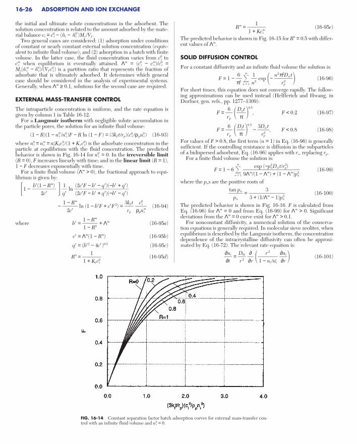
the initial and ultimate solute concentrations in the adsorbent. Thesolution concentration is related to the amount adsorbed by the mate-rial balance ci = c i
0 − (ni − ni0′)Ms /Vf .
Two general cases are considered: (1) adsorption under conditionsof constant or nearly constant external solution concentration (equiv-alent to infinite fluid volume); and (2) adsorption in a batch with finitevolume. In the latter case, the fluid concentration varies from c i
0 to c i
∞ when equilibrium is eventually attained. Λ∞ = (c i0 − c i
∞)/c i0 =
Ms(n i∞ − n i
0)/(Vf c i0 ) is a partition ratio that represents the fraction of
adsorbate that is ultimately adsorbed. It determines which generalcase should be considered in the analysis of experimental systems.Generally, when Λ∞ ≥ 0.1, solutions for the second case are required.
EXTERNAL MASS-TRANSFER CONTROL
The intraparticle concentration is uniform, and the rate equation isgiven by column 1 in Table 16-12.
For a Langmuir isotherm with negligible solute accumulation inthe particle pores, the solution for an infinite fluid volume:
(1 − R)(1 − n i0′/ni
0 )F − R ln (1 − F) = (3kf t/rp)(c i0 /ρpn i
0 ) (16-93)
where ni0 = ni
∞ = nisKic i
0 /(1 + K ic i0) is the adsorbate concentration in the
particle at equilibrium with the fluid concentration. The predictedbehavior is shown in Fig. 16-14 for ni
0′ = 0. In the irreversible limit(R = 0), F increases linearly with time; and in the linear limit (R = 1),1 − F decreases exponentially with time.
For a finite fluid volume (Λ∞ > 0), the fractional approach to equi-librium is given by:
1 − ln
− ln (1 − b′F + c′F 2) = (16-94)
where b′ = + Λ∞ (16-95a)
c′ = Λ∞(1 − R∞) (16-95b)
q′ = (b′2 − 4c′ )0.5 (16-95c)
R0 = (16-95d)1
1 + Kici
0
1 − R∞
1 − R0
ci0
ρpni
∞
3kf trp
1 − R∞
2c′
(2c′F − b′ − q′)(−b′ + q′)(2c′F − b′ + q′)(−b′ − q′)
1q′
b′(1 − R∞)
2c′
R∞ = (16-95e)
The predicted behavior is shown in Fig. 16-15 for R0 = 0.5 with differ-ent values of Λ∞.
SOLID DIFFUSION CONTROL
For a constant diffusivity and an infinite fluid volume the solution is:
F = 1 − ∞
n = 1
exp − (16-96)
For short times, this equation does not converge rapidly. The follow-ing approximations can be used instead (Helfferich and Hwang, inDorfner, gen. refs., pp. 1277–1309):
F = 0.5
, F < 0.2 (16-97)
F = 0.5
− , F < 0.8 (16-98)
For values of F > 0.8, the first term (n = 1) in Eq. (16-96) is generallysufficient. If the controlling resistance is diffusion in the subparticlesof a bidispersed adsorbent, Eq. (16-96) applies with rs, replacing rp.
For a finite fluid volume the solution is:
F = 1 − 6 ∞
n = 1
(16-99)
where the pns are the positive roots of
= (16-100)
The predicted behavior is shown in Fig. 16-16. F is calculated fromEq. (16-96) for Λ∞ = 0 and from Eq. (16-99) for Λ∞ > 0. Significantdeviations from the Λ∞ = 0 curve exist for Λ∞ > 0.1.
For nonconstant diffusivity, a numerical solution of the conserva-tion equations is generally required. In molecular sieve zeolites, whenequilibrium is described by the Langmuir isotherm, the concentrationdependence of the intracrystalline diffusivity can often be approxi-mated by Eq. (16-72). The relevant rate equation is:
= (16-101)∂ni∂r
r 2
1 − ni /ni
s
∂∂r
D0ir 2
∂ni∂t
33 + (1/Λ∞ − 1)pn
2
tan pn
pn
exp (−pn2 Dsi t/r2
p)9Λ∞/(1 − Λ∞) + (1 − Λ∞)pn
2
3Dsi t
r2p
Dstπ
6rp
Dsit
π6
rp
n2π2Dsi t
r2p
1n2
6π2
11 + Kci
∞
16-26 ADSORPTION AND ION EXCHANGE
FIG. 16-14 Constant separation factor batch adsorption curves for external mass-transfer con-trol with an infinite fluid volume and ni
0 = 0.
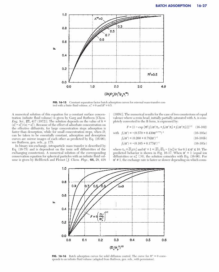
A numerical solution of this equation for a constant surface concen-tration (infinite fluid volume) is given by Garg and Ruthven [Chem.Eng. Sci., 27, 417 (1972)]. The solution depends on the value of λ =(ni
0 − ni0′)/(ni
s − ni0′). Because of the effect of adsorbate concentration on
the effective diffusivity, for large concentration steps adsorption isfaster than desorption, while for small concentration steps, when Ds
can be taken to be essentially constant, adsorption and desorptioncurves are mirror images of each other as predicted by Eq. (16-96);see Ruthven, gen. refs., p. 175.
In binary ion-exchange, intraparticle mass transfer is described byEq. (16-75) and is dependent on the ionic self diffusivities of theexchanging counterions. A numerical solution of the correspondingconservation equation for spherical particles with an infinite fluid vol-ume is given by Helfferich and Plesset [ J. Chem. Phys., 66, 28, 418
(1958)]. The numerical results for the case of two counterions of equalvalence where a resin bead, initially partially saturated with A, is com-pletely converted to the B form, is expressed by:
F = 1 − exp [π2( f1(α′ )τD + f2(α′ )τD2 + f3(α′ )τD
3 )]1/2 (16-102)
with f1(α′ ) = −(0.570 + 0.430α′ 0.775)−1 (16-103a)
f2(α′ ) = (0.260 + 0.782α′ )−1 (16-103b)
f3(α′ ) = −(0.165 + 0.177α′ )−1 (16-103c)
where τD = DAt/rp2 and α′ = 1 + (DA /DB − 1)nA
0′/ns for 0.1 ≤ α′ ≤ 10. Thepredicted behavior is shown in Fig. 16-17. When α′ = 1 (equal ion diffusivities or nA
0′ ∼ 0), the solution coincides with Eq. (16-96). For α′ ≠ 1, the exchange rate is faster or slower depending on which coun-
BATCH ADSORPTION 16-27
FIG. 16-15 Constant separation factor batch adsorption curves for external mass-transfer con-trol with a finite fluid volume, ni
0′ = 0 and R0 = 0.5.
FIG. 16-16 Batch adsorption curves for solid diffusion control. The curve for Λ∞ = 0 corre-sponds to an infinite fluid volume (adapted from Ruthven, gen. refs., with permission).

terion is initially present in the ion exchanger and on the initial level of saturation.
For an initially fully saturated particle, the exchange rate is fasterwhen the faster counterion is initially in the resin, with the differencein rate becoming more important as conversion from one form to theother progresses. Helfferich (gen. refs., pp. 270–271) gives explicitexpressions for the exchange of ions of unequal valence.
PORE DIFFUSION CONTROL
The rate equation is given by item A in Table 16-11. With pore fluidand adsorbent at equilibrium at each point within the particle and fora constant diffusivity, the rate equation can be written as:
= r 2 (16-104)
For a linear isotherm (ni = Kici), this equation is identical to the con-servation equation for solid diffusion, except that the solid diffusivityDsi is replaced by the equivalent diffusivity Dei = εpDpi /(εp + ρpKi).Thus, Eqs. (16-96) and (16-99) can be used for pore diffusion controlwith infinite and finite fluid volumes simply by replacing Dsi with Dei.
When the adsorption isotherm is nonlinear, a numerical solution isgenerally required. For a Langmuir system with negligible soluteholdup in the pore fluid, item A in Table 16-11 gives:
= (16-105)
This equation has the same form of that obtained for solid diffusioncontrol with Dsi replaced by the equivalent concentration-dependentdiffusivity Dei = εpDpi /[ρpn i
sKi(1 − ni /nis)2]. Numerical results for the
case of adsorption on an initially clean particle are given in Fig. 16-18for different values of λ = ni
0/nis = 1 − R. The uptake curves become
increasingly steeper, as the nonlinearity of the isotherm, measured bythe parameter λ, increases. The desorption curve shown for a particlewith ni
0′/nis = 0.9 shows that for the same step in concentration, adsorp-
tion occurs much more quickly than desorption. This difference, how-ever, becomes smaller as the value of λ is reduced and in the linearregion of the adsorption isotherm (λ → 0), adsorption and desorptioncurves are mirror images. The solution in Fig. 16-18 is applicable to anonzero initial adsorbent loading by redefining λ as (ni
0 − ni0′)/(ni
s − n0′)
∂ni∂r
r 2
(1 − ni /ni
s)2
∂∂r
1r 2
εpDpiρpn i
sKi
∂ni∂t
∂cpi∂r
∂∂r
1r 2
εpDpiεp + ρp dni
e /dci
∂cpi∂t
and the dimensionless time variable as [εpDpit/ρp(1 − ni0′/ni
s)2nisK ir p
2]1/2
(Ruthven, gen. refs.).In the irreversible limit (R < 0.1), the adsorption front within the
particle approaches a shock transition separating an inner core intowhich the adsorbate has not yet penetrated from an outer layer inwhich the adsorbed phase concentration is uniform at the saturationvalue. The dynamics of this process is described approximately by theshrinking-core model [Yagi and Kunii, Chem. Eng. (Japan), 19, 500(1955)]. For an infinite fluid volume, the solution is:
= − F − (1 − F)2/3 (16-106)
or, in explicit form [Brauch and Schlunder, Chem. Eng. Sci., 30, 540(1975)]:
F = 1 − + cos + cos−1 1 − 3
(16-107)
For a finite fluid volume with 0 < Λ∞ ≤ 1, the solution is [Teo andRuthven, Ind. Eng. Chem. Process Des. Dev., 25, 17 (1986)]:
= I2 − I1 (16-108)
where
I1 = tan−1 − tan−1 + ln 3
(16-109a)
I2 = ln (16-109b)
η = (1 − F)1/3 (16-109c)
λ′ = − 11/3
(16-109d)
COMBINED RESISTANCES
In general, exact analytic solutions are available only for the linear (R = 1) and irreversible limits (R → 0). Intermediate cases require
1Λ∞
λ′ 3 + η3
λ′ 3 + 1
13Λ∞
λ′ + 1λ′ + η
λ′ 3 + η3
λ′ 3 + 1
16λ′Λ ∞
2 − λ′λ′3
2η − λ′λ′3
1λ′Λ ∞3
c i0
ρpni
s
εpDpit
rp2
ci0
ρpni
s
12εpDpi t
rp2
13
π3
12
12
13
12
ci0
ρpni
s
εpDpit
rp2
16-28 ADSORPTION AND ION EXCHANGE
FIG. 16-17 Batch ion exchange for two equal-valence counterions. The exchanger is initiallyuniformly loaded with ion A in concentration nA
0′ and is completely converted to the B form. α′ = 1 + (DA /DB − 1)nA
0′/ns.

numerical solution or use of approximate driving force expressions(see “Rate and Dispersion Factors”).
Parallel Pore and Solid Diffusion Control With a linearisotherm, assuming equilibrium between the pore fluid and thesolid adsorbent, batch adsorption can be represented in terms of anequivalent solid diffusivity Dei = (εpDpi + ρp Dsi)/(εp + ρp Ki). Thus,Eqs. (16-96) and (16-99) can be used for this case with Dsi replacedby Dei.
External Mass Transfer and Intraparticle Diffusion ControlWith a linear isotherm, the solution for combined external masstransfer and pore diffusion control with an infinite fluid volume is(Crank, Mathematics of Diffusion, 2d ed., Clarendon Press, 1975):
F = 1 − ∞
n = 1
(16-110)
where Bi = kf rp /εpDpi is the Biot number and the pns are the positiveroots of
pn cot pn = 1 − Bi (16-111)
For a finite fluid volume the solution is:
F = 1 − 6 ∞
n = 1
(16-112)
where the pns are the positive roots of
= (16-113)
These expressions can also be used for the case of external mass trans-fer and solid diffusion control by substituting Dsi for εpDpi /(εp + ρpKi)and kf rp /(ρpKiDsi) for the Biot number.
In the irreversible limit, the solution for combined external resis-tance and pore diffusion with infinite fluid volume is (Yagi and Kunii):
= − 1 − F − (1 − F)2/3 (16-114)12
1Bi
13
12
ci0
ρpni
s
εpDpi t
rp2
3 − 1 −
Λ∞
Λ∞
pB
n
i
2
3 + 1 −
Λ∞
Λ∞
(Bi −
B1i)pn
2
tan pn
pn
exp [−(pn2εpDpi t/r p
2)/(εp + ρpKi)]
1
9−ΛΛ
∞
∞ + (1 − Λ∞)pn2 − (5Λ∞ + 1)
pB
n
i
2
+ (1 − Λ∞) Bpin4
2
6Bi2 exp [−(pn2εpDpi t/r p
2)/(εp + ρpKi)]
pn2 [pn
2 + Bi(Bi − 1)]
For a finite fluid volume the solution is (Teo and Ruthen):
= 1 − I2 − I1 (16-115)
where I1 and I2 are given be Eqs. (16-109a) and (16-109b).Bidispersed Particles For particles of radius rp comprising
adsorptive subparticles of radius rs that define a macropore network,conservation equations are needed to describe transport both withinthe macropores and within the subparticles and are given in Table 16-11, item D. Detailed equations and solutions for a linear isothermare given in Ruthven (gen. refs., p. 183) and Ruckenstein et al. [Chem.Eng. Sci., 26, 1306 (1971)]. The solution for a linear isotherm withno external resistance and an infinite fluid volume is:
F = 1 − ∞
m = 1∞
n = 1
(16-116)
where the pn, m values are the roots of the equation
αp2n, m − n2π2 = β(pn, m cot pn, m − 1) (16-117)
and α = (16-118a)
β = (16-118b)
In these equations, Dsi is the diffusivity in the subparticles, and Dpi isthe diffusivity in the pore network formed by the subparticles.
For large Ki values, the uptake curve depends only upon the valueof the parameter β representing the ratio of characteristic time con-stants for diffusion in the pores and in the subparticles. For small βvalues, diffusion in the subparticles is controlling and the solutioncoincides with Eq. (16-96) with rs replacing rp. For large β values,pore diffusion is controlling, and the solution coincides with Eq. (16-96) with εpDpi /(εp + ρpKi) replacing Dsi.
Lee [AIChE J., 24, 531 (1978)] gives the solution for batch adsorp-tion with bidispersed particles for the case of a finite fluid volume.
3αρpKi
εp
Dsi /r s2
Dpi /rp
2
exp(−p2n, mDsi t/r s
2)
α + β2
1 + co
pt
n
p
, m
n, m (pn, m cot pn, m − 1)
n2π2
p4
n, m
18β + 3α
1Bi
ci0
ρpni
s
εpDpi t
rp2
BATCH ADSORPTION 16-29
FIG. 16-18 Constant separation factor batch adsorption curves for pore diffusion control withan infinite fluid volume. λ is defined in the text.

As discussed in “Design Concepts,” a large fraction of adsorption andion-exchange processes takes place in fixed beds. Two classical meth-ods for analyzing fixed-bed transitions are described here. First, localequilibrium theory is presented. In this, all mass-transfer resistancesare ignored to focus on the often dominating role of isotherm shape.Second, results of constant pattern analysis are presented. This givesthe maximum breadth to which a mass-transfer zone will spread forvarious rate mechanisms. It is therefore conservative for design pur-poses. Both of these methods pertain to behavior in deep beds. Forshallow beds, the equations given below must be solved for the partic-ular case of interest.
DIMENSIONLESS SYSTEM
For the methods, we consider Eq. (16-52), the material balance for afixed bed, written in the form
ρb + εb + ε = εDL c (16-119)
where it has been assumed that DL is constant and that ci ≈ ci (or thatthe second term in the balance is small compared to the first—usuallya good assumption).
Dimensionless variables can be defined for time, the axial coordi-nate, and velocity:
τ = (16-120)
ζ = (16-121)
v* = (16-122)
where L is bed length, vref is the interstitial velocity at the bed inlet,and τ is equal to the number of empty bed volumes of feed passed intothe bed. The material balance becomes
ρb + εb + = c (16-123)
where NPe = εvrefL/DL is a Peclet number for the bed or a number ofdispersion units. Equation (16-123) or a similar equation is often thematerial balance used in nonisothermal problems, in problems involv-ing adsorption of nontrace components, and in calculations of cycles.
For a trace, isothermal system, we have v* = 1, and using thedimensionless system variables for concentrations [Eq. (16-10)], Eq.(16-123) becomes
Λ + εb + = (16-124)
where Λ is the partition ratio defined by
Λ = (16-125)
This important dimensionless group is the volumetric capacity of thebed for the sorbable component divided by the concentration of thesorbable component in the feed. The stoichiometric capacity of the bed for solute is exactly equal to Λ empty bed volumes of feed (tosaturate the sorbent at the feed concentration) plus a fraction of a bedvolume of feed to fill the voids outside and inside the particles. Alter-natively, we also obtain Eq. (16-124) using the dimensionless transi-tion variables for concentrations [Eq. (16-11)], but now the partitionratio in the first term of Eq. (16-124) pertains to the transition and isgiven by
Λ = ρb (16-126)
Equation (16-124) is a commonly used form of material balance for afixed-bed adsorber.
n″i − n′ic″i − c′i
ρbn iref
c i
ref
∂2c*i∂ζ2
1NPe
∂c*i∂ζ
∂c*i∂τ
∂n*i∂τ
∂yi∂ζ
∂∂ζ
1NPe
∂(v*ci)
∂ζ∂ci∂τ
∂ni∂τ
vvref
zL
εvreft
L
∂yi∂z
∂∂z
∂(vci)
∂z∂ci∂t
∂ni∂t
If the system under consideration involves use of the sorbent foronly a single feed step or reuse after uniform regeneration, as in manyapplications with activated carbons and ion exchangers, then one oftwo paths is often followed at this point to simplify Eq. (16-124) fur-ther. The second term on the left-hand side of the equation is oftenassumed to be negligibly small (usually a good assumption), and timeis redefined as
τ1 = (16-127)
to give + = (16-128)
Alternatively, in the absence of axial dispersion, a variable of the form
τ1 = (16-129)
can be defined to reduce Eq. (16-124) directly to
+ = 0 (16-130)
The variable τ1 defined by Eq. (16-127) or (16-129) is a through-put parameter, equal to unity (hence, the “1” subscript) at the timewhen the stoichiometric center of the concentration wave leaves thebed. This important group, in essence a dimensionless time variable,essentially determines the location of the stoichiometric center of thetransition in the bed at any time.
LOCAL EQUILIBRIUM THEORY
In local equilibrium theory, fluid and sorbed phases are assumed to bein local equilibrium with one another at every axial position in the bed.Thus, because of uniform concentrations, the overbar on n*i is not nec-essary and we have ci ≈ ci [note Eqs. (16-52) and (16-119)].
Single Transition System For a system described by a singlematerial balance, Eq. (16-130) gives
= − = (16-131)
where dτ1/dζ is the reciprocal of a concentration velocity. Equation(16-131) is the equation for a simple wave (or gradual transition orproportionate pattern). If a bed is initially uniformly saturated, thendτ1 /dζ = τ1 /ζ. Thus, for the dimensionless system, the reciprocal ofthe velocity of a concentration is equal to the slope of the isotherm atthat concentration. Furthermore, from Eq. (16-131), the depth ofpenetration of a given concentration into the bed is directly propor-tional to time, so the breadth of a simple wave increases in direct pro-portion to the depth of its penetration into the bed (or to time). Thus,for the simple wave, the length of the MTZ is proportional to thedepth of the bed through which the wave has passed. Consideration ofisotherm shape indicates that a simple wave occurs for an unfavorabledimensionless isotherm (d 2n*i /dc*i 2 > 0), for which low concentrationswill go faster than high concentrations. Equation (16-131) also per-tains to a linear isotherm, in which case the wave is called a contactdiscontinuity, because it has neither a tendency to spread norsharpen. If mass-transfer resistance is added to the consideration ofwave character for unfavorable isotherms, the wave will still asymp-totically approach the simple wave result given by Eq. (16-131).
For a favorable isotherm (d 2n*i /dc*i 2 < 0), Eq. (16-131) gives theimpossible result that three concentrations can coexist at one point inthe bed (see example below). The correct solution is a shock (orabrupt transition) and not a simple wave. Mathematical theory hasbeen developed for this case to give “weak solutions” to conservationlaws. The form of the solution is
shock speed = change in fluxchange in accumulated quantity
dn*idc*i
∂c*i /∂ζ∂c*i /∂τ1
dτ1dζ
∂c*i∂ζ
∂n*i∂τ1
τ − εbζ
Λ
∂2c*i∂ζ2
1NPe
∂c*i∂ζ
∂n*i∂τ1
τΛ
16-30 ADSORPTION AND ION EXCHANGE
FIXED-BED TRANSITIONS
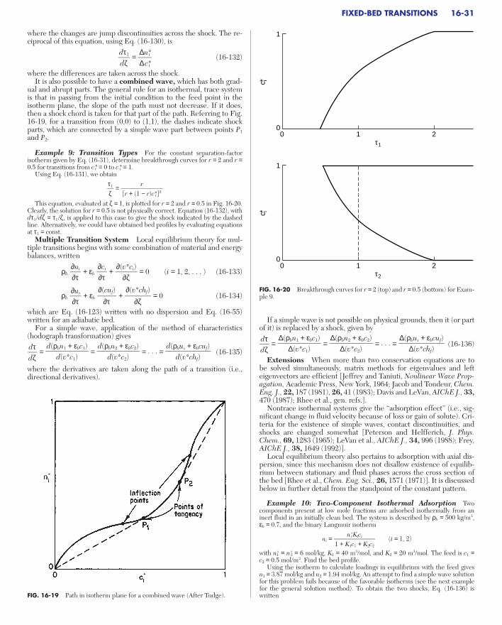
where the changes are jump discontinuities across the shock. The re-ciprocal of this equation, using Eq. (16-130), is
= (16-132)
where the differences are taken across the shock.It is also possible to have a combined wave, which has both grad-
ual and abrupt parts. The general rule for an isothermal, trace systemis that in passing from the initial condition to the feed point in theisotherm plane, the slope of the path must not decrease. If it does,then a shock chord is taken for that part of the path. Referring to Fig.16-19, for a transition from (0,0) to (1,1), the dashes indicate shockparts, which are connected by a simple wave part between points P1
and P2.
Example 9: Transition Types For the constant separation-factorisotherm given by Eq. (16-31), determine breakthrough curves for r = 2 and r =0.5 for transitions from c*i = 0 to c*i = 1.
Using Eq. (16-131), we obtain
=
This equation, evaluated at ζ = 1, is plotted for r = 2 and r = 0.5 in Fig. 16-20.Clearly, the solution for r = 0.5 is not physically correct. Equation (16-132), withdτ1 /dζ = τ1 /ζ, is applied to this case to give the shock indicated by the dashedline. Alternatively, we could have obtained bed profiles by evaluating equationsat τ1 = const.
Multiple Transition System Local equilibrium theory for mul-tiple transitions begins with some combination of material and energybalances, written
ρb + εb + = 0 (i = 1, 2, . . . ) (16-133)
ρb + εb + = 0 (16-134)
which are Eq. (16-123) written with no dispersion and Eq. (16-55)written for an adiabatic bed.
For a simple wave, application of the method of characteristics(hodograph transformation) gives
= = = . . . = (16-135)
where the derivatives are taken along the path of a transition (i.e.,directional derivatives).
d(ρbus + εbcuf)
d(v*chf)d(ρbn2 + εbc2)
d(v*c2)d(ρbn1 + εbc1)
d(v*c1)dτdζ
∂(v*chf)
∂ζ∂(cuf)
∂τ∂us∂τ
∂(v*ci)
∂ζ∂ci∂τ
∂ni∂τ
r[r + (1 − r)c*i ]2
τ1ζ
∆n*i∆c*i
dτ1dζ
If a simple wave is not possible on physical grounds, then it (or partof it) is replaced by a shock, given by
= = = . . . = (16-136)
Extensions When more than two conservation equations are tobe solved simultaneously, matrix methods for eigenvalues and lefteigenvectors are efficient [Jeffrey and Taniuti, Nonlinear Wave Prop-agation, Academic Press, New York, 1964; Jacob and Tondeur, Chem.Eng. J., 22, 187 (1981), 26, 41 (1983); Davis and LeVan, AIChE J., 33,470 (1987); Rhee et al., gen. refs.].
Nontrace isothermal systems give the “adsorption effect” (i.e., sig-nificant change in fluid velocity because of loss or gain of solute). Cri-teria for the existence of simple waves, contact discontinuities, andshocks are changed somewhat [Peterson and Helfferich, J. Phys.Chem., 69, 1283 (1965); LeVan et al., AIChE J., 34, 996 (1988); Frey,AIChE J., 38, 1649 (1992)].
Local equilibrium theory also pertains to adsorption with axial dis-persion, since this mechanism does not disallow existence of equilib-rium between stationary and fluid phases across the cross section ofthe bed [Rhee et al., Chem. Eng. Sci., 26, 1571 (1971)]. It is discussedbelow in further detail from the standpoint of the constant pattern.
Example 10: Two-Component Isothermal Adsorption Twocomponents present at low mole fractions are adsorbed isothermally from aninert fluid in an initially clean bed. The system is described by ρb = 500 kg/m3, εb = 0.7, and the binary Langmuir isotherm
ni = (i = 1, 2)
with n1s = n 2
s = 6 mol/kg, K1 = 40 m3/mol, and K2 = 20 m3/mol. The feed is c1 =c2 = 0.5 mol/m3. Find the bed profile.
Using the isotherm to calculate loadings in equilibrium with the feed gives n1 = 3.87 mol/kg and n2 = 1.94 mol/kg. An attempt to find a simple wave solutionfor this problem fails because of the favorable isotherms (see the next examplefor the general solution method). To obtain the two shocks, Eq. (16-136) is written
nisKici
1 + K1c1 + K2c2
∆(ρbus + εbcuf)
∆(v*chf)∆(ρbn2 + εbc2)
∆(v*c2)∆(ρbn1 + εbc1)
∆(v*c1)dτdζ
FIXED-BED TRANSITIONS 16-31
1
00 1 2
τ1
c i*c i*
1
00 1 2
τ2
FIG. 16-20 Breakthrough curves for r = 2 (top) and r = 0.5 (bottom) for Exam-ple 9.
FIG. 16-19 Path in isotherm plane for a combined wave (After Tudge).

= =
The concentration of one of the components will drop to zero in the shocknearest the bed inlet. If it is component 1, then using feed values and the equa-tion above, that shock would be at
= ≈ = 3870
Similarly, if the second component were to disappear in the first shock, wewould have τ /ζ = 1940. Material balance considerations require that we acceptthe shorter distance, so component 1 disappears in the first shock.
The concentrations of component 2 on the plateau downstream of the firstshock are then calculated from
= ≈ = 3870
and its pure component isotherm, giving c2 = 0.987 mol/m3 and n2 = 5.71 mol/kg.The location of this shock is determined using these concentrations and
= ≈
which gives τ /ζ = 2890. The bed profile is plotted in Fig. 16-21 using ζ /τ as theabsissa. (This example can also be worked with the h-transformation describedin this section under chromatography.)
Example 11: Adiabatic Adsorption and Thermal RegenerationAn initially clean activated carbon bed at 320 K is fed a vapor of benzene innitrogen at a total pressure of 1 MPa. The concentration of benzene in the feedis 6 mol/m3. After the bed is uniformly saturated with feed, it is regeneratedusing benzene-free nitrogen at 400 K and 1 MPa. Solve for both steps. For sim-plicity, neglect fluid-phase accumulation terms and assume constant mean heatcapacities for stationary and fluid phases and a constant velocity. The system isdescribed by
ρbn1 =
ρbn1s = 2750 mol/m3
K1 = 3.88 × 10⁻⁸T exp [q1st /(ℜ T)] m3/(mol K1/2)
ρbCsm = 850 kJ/(m3 K)
cCpfm = 11.3 kJ/(m3 K)
q1st = 43.5 kJ/mol
T ref = 320 K
Extensive analysis has been made of this system [Rhee et al., Chem. Eng. J., 1,241 (1970) and gen. refs.; LeVan, in Rodrigues et al., gen. refs.].
To obtain the concentration and temperature profiles, the two transitions arefirst assumed to be gradual. Equation (16-135) is written in the form
= ρb = ρb
where, from Eqs. (16-56) to (16-60),
ρbus = ρbCsm(T − T ref ) − ρbn1q1st
chf = cCpfm(T − T ref )
dusd(chf)
dn1dc1
τζ
ρbn1sK1c1
1 + K1c1
ρbn2
c2
ρbn2 + εbc2
c2
τζ
ρb∆n2
∆c2
∆(ρbn2 + εbc2)
∆c2
τζ
ρbn1
c1
ρbn1 + εbc1
c1
τζ
∆(ρbn2 + εbc2)
∆c2
∆(ρbn1 + εbc1)
∆c1
dτdζ
This equation is expanded in terms of c1 and T to obtain
= ρb + = − + Solving the rightmost equality for the directional derivative using the quadraticformula gives
=
with a = b = − +
d =
The plus sign corresponds to the downstream transition and the minus sign tothe upstream one. This equation is solved along each path beginning at therespective end points—the initial condition of the bed for the downstream tran-sition and the feed condition for the upstream transition. If either path fails toevolve continuously in the expected direction, the difference form, from Eq.(16-136),
= ρb = ρb
is used for that path (or part thereof, if appropriate); two solutions of this equa-tion pass through each composition point, and care must be taken to ensure thatthe correct path is taken. The two correct paths found intersect to give the com-position and temperature of an intermediate plateau region.
Letting c1ref = 6 mol/m3, the isotherm gives ρbn1
ref = 2700 mol/m3, and the par-tition ratio is Λ = 450.
In the figures, Γ(k) and Σ(k) symbolize simple waves and shocks, respectively,with k = 1 downstream and k = 2 upstream.
Adiabatic Adsorption The construction is shown in Figs. 16-22 and 16-23.The first path begins at the initial condition, point A (T = 320 K, c1 = 0 mol/m3).Since ∂n1 /∂T = 0 there, we obtain dc1/dT = 0 and τ /ζ = ρbCsm /(cCpfm) = 75.2 (orτ/Λ = 0.167 at ζ = 1), corresponding to a pure thermal wave along the c1 = 0 axisof Fig. 16-22. The second path begins at the feed condition, point B (T = 320 K,c1 = 6 mol/m3). A Γ(2) fails, so a Σ(2) is calculated and plotted in the two figures.The Γ(1) and Σ(2) intersect at point C (T = 348 K, c1 = 0 mol/m3) Breakthroughcurves of temperature and concentration are shown in Fig. 16-24.
Thermal Regeneration The bed, initially at point B, is fed with pure nitro-gen. The feed, at point D (T = 400 K, c1 = 0 mol/m3), provides a successful Γ(2).The Γ(1) from point B fails, so a Σ(1), which differs imperceptibly from Γ(1), isdetermined. The Σ(1) and Γ(2) meet at point E (T = 320.8 K, c1 = 8.93 mol/m3),where ρbn1 = 2716 mol/m3, which is greater than the initial loading, indicating“roll-up,” a term attributed to Basmadjian et al. [Ind. Eng. Chem. Process Des.Dev., 14, 328 (1975)], of the adsorbed-phase concentration. Breakthroughcurves are shown in Fig. 16-25. The Σ(1) leaves the bed at τ /Λ = 0.011. The Γ(2) begins to emerge at τ /Λ = 0.169, but regeneration is not complete until τ/Λ = 2.38.
It is possible (with lower initial bed temperature, higher initial loading, orhigher regeneration temperature or pressure) for the transition paths to contactthe saturated vapor curve in Fig. 16-22 rather than intersect beneath it. For thiscase, liquid benzene condenses in the bed, and the effluent vapor is saturatedduring part of regeneration [Friday and LeVan, AIChE J., 30, 679 (1984)].
CONSTANT PATTERN BEHAVIOR FOR FAVORABLE ISOTHERMS
With a favorable isotherm and a mass-transfer resistance or axial dis-persion, a transition approaches a constant pattern, which is anasymptotic shape beyond which the wave will not spread. The wave issaid to be “self-sharpening.” (If a wave is initially broader than theconstant pattern, it will sharpen to approach the constant pattern.)Thus, for an initially uniformly loaded bed, the constant pattern givesthe maximum breadth of the MTZ. As bed length is increased, theconstant pattern will occupy an increasingly smaller fraction of thebed. (Square-root spreading for a linear isotherm gives this same qual-itative result.)
The treatment here is restricted to the Langmuir or constant sepa-ration factor isotherm, single-component adsorption, dilute systems,isothermal behavior, and mass-transfer resistances acting alone. Ref-erences to extensions are given below. Different isotherms have beenconsidered, and the theory is well understood for general isotherms.
∆us∆(chf)
∆n1∆c1
dτdζ
ρb∂n1
∂T
ρb∂n1
∂c1
ρbCsm(cCpfm)
∂n1∂T
ρbq1st
(cCpfm)
∂n1∂c1
ρbq1st
(cCpfm)
−b b2− 4ad
2adc1dT
dc1dT
∂n1∂c1
∂n1∂T
ρbq1st
cCpfm
ρbCsmcCpfm
dTdc1
∂n1∂T
∂n1∂c1
τζ
16-32 ADSORPTION AND ION EXCHANGE
ci*
1.0
0.5
00 1 3 42 5
ζ /τ × 104
c2*
c1* & c2*
FIG. 16-21 Bed profiles for two-component isothermal adsorption, Exam-ple 10.
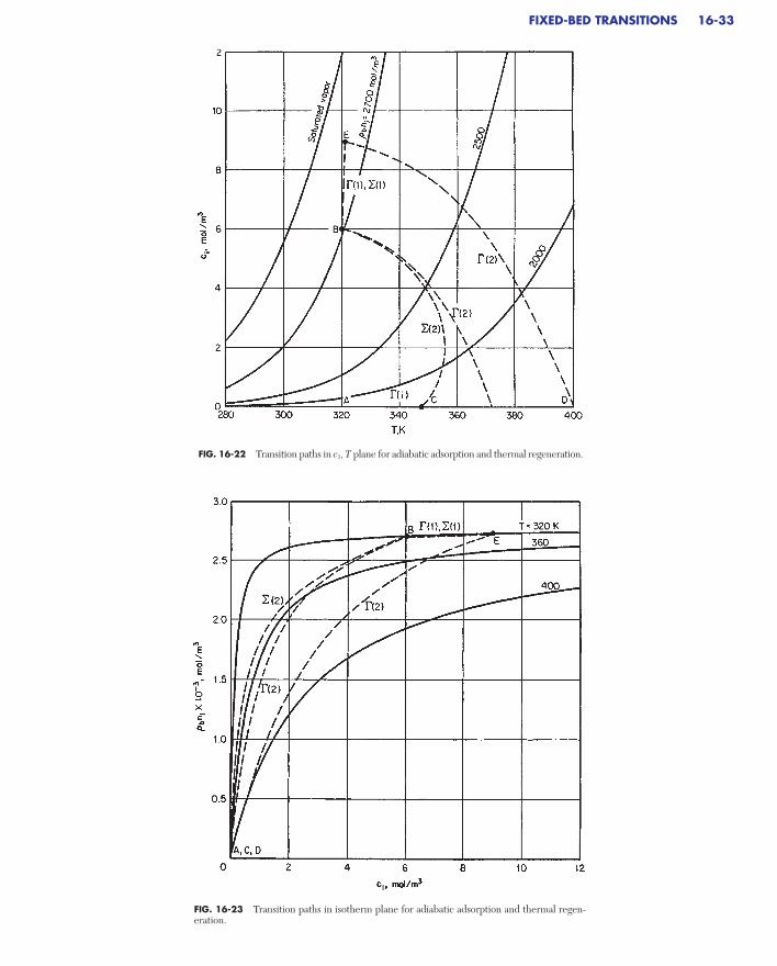
FIXED-BED TRANSITIONS 16-33
FIG. 16-22 Transition paths in c1, T plane for adiabatic adsorption and thermal regeneration.
FIG. 16-23 Transition paths in isotherm plane for adiabatic adsorption and thermal regen-eration.
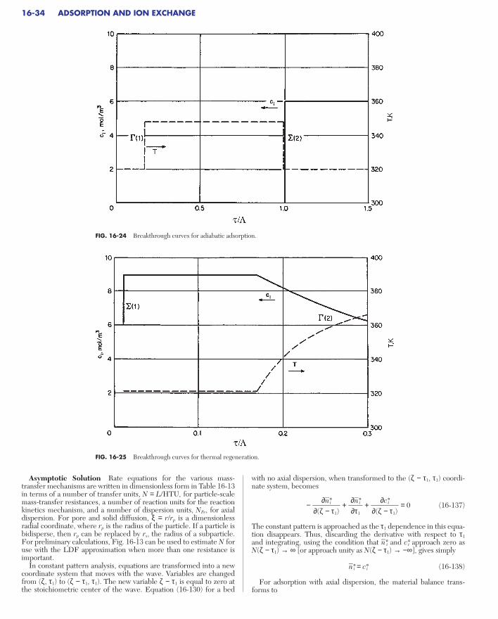
Asymptotic Solution Rate equations for the various mass-transfer mechanisms are written in dimensionless form in Table 16-13in terms of a number of transfer units, N = L/HTU, for particle-scalemass-transfer resistances, a number of reaction units for the reactionkinetics mechanism, and a number of dispersion units, NPe, for axialdispersion. For pore and solid diffusion, ξ = r/rp is a dimensionlessradial coordinate, where rp is the radius of the particle. If a particle isbidisperse, then rp can be replaced by rs, the radius of a subparticle.For preliminary calculations, Fig. 16-13 can be used to estimate N foruse with the LDF approximation when more than one resistance isimportant.
In constant pattern analysis, equations are transformed into a newcoordinate system that moves with the wave. Variables are changedfrom (ζ, τ1) to (ζ − τ1, τ1). The new variable ζ − τ1 is equal to zero atthe stoichiometric center of the wave. Equation (16-130) for a bed
with no axial dispersion, when transformed to the (ζ − τ1, τ1) coordi-nate system, becomes
− + + =0 (16-137)
The constant pattern is approached as the τ1 dependence in this equa-tion disappears. Thus, discarding the derivative with respect to τ1
and integrating, using the condition that n*i and c*i approach zero as N(ζ − τ1) → ∞ [or approach unity as N(ζ − τ1) → −∞], gives simply
n*i = c*i (16-138)
For adsorption with axial dispersion, the material balance trans-forms to
∂c*i∂(ζ − τ1)
∂n*i∂τ1
∂n*i∂(ζ − τ1)
16-34 ADSORPTION AND ION EXCHANGE
FIG. 16-24 Breakthrough curves for adiabatic adsorption.
FIG. 16-25 Breakthrough curves for thermal regeneration.
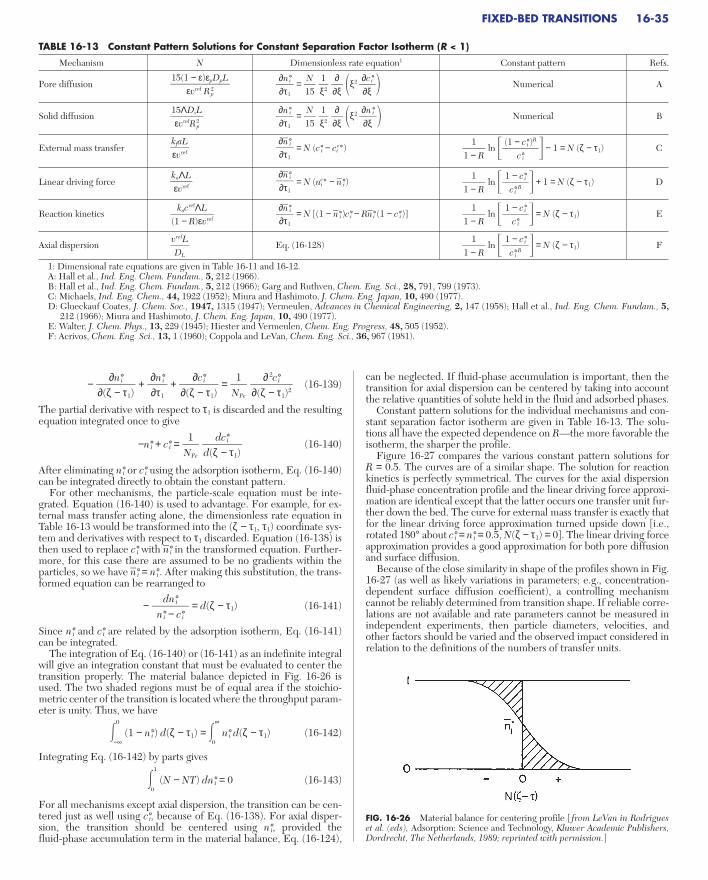
− + + = (16-139)
The partial derivative with respect to τ1 is discarded and the resultingequation integrated once to give
−n*i + c*i = (16-140)
After eliminating n*i or c*i using the adsorption isotherm, Eq. (16-140)can be integrated directly to obtain the constant pattern.
For other mechanisms, the particle-scale equation must be inte-grated. Equation (16-140) is used to advantage. For example, for ex-ternal mass transfer acting alone, the dimensionless rate equation inTable 16-13 would be transformed into the (ζ − τ1, τ1) coordinate sys-tem and derivatives with respect to τ1 discarded. Equation (16-138) isthen used to replace c*i with n*i in the transformed equation. Further-more, for this case there are assumed to be no gradients within theparticles, so we have n*i = n*i . After making this substitution, the trans-formed equation can be rearranged to
− = d(ζ − τ1) (16-141)
Since n*i and c*i are related by the adsorption isotherm, Eq. (16-141)can be integrated.
The integration of Eq. (16-140) or (16-141) as an indefinite integralwill give an integration constant that must be evaluated to center thetransition properly. The material balance depicted in Fig. 16-26 isused. The two shaded regions must be of equal area if the stoichio-metric center of the transition is located where the throughput param-eter is unity. Thus, we have
0
−∞(1 − n*i) d(ζ − τ1) = ∞
0n*i d(ζ − τ1) (16-142)
Integrating Eq. (16-142) by parts gives
1
0(N − NT) dn*i = 0 (16-143)
For all mechanisms except axial dispersion, the transition can be cen-tered just as well using c*i, because of Eq. (16-138). For axial disper-sion, the transition should be centered using n*i, provided thefluid-phase accumulation term in the material balance, Eq. (16-124),
dn*in*i − c*i
dc*id(ζ − τ1)
1NPe
∂ 2c*i∂(ζ − τ1)2
1NPe
∂c*i∂(ζ − τ1)
∂n*i∂τ1
∂n*i∂(ζ − τ1)
can be neglected. If fluid-phase accumulation is important, then thetransition for axial dispersion can be centered by taking into accountthe relative quantities of solute held in the fluid and adsorbed phases.
Constant pattern solutions for the individual mechanisms and con-stant separation factor isotherm are given in Table 16-13. The solu-tions all have the expected dependence on R—the more favorable theisotherm, the sharper the profile.
Figure 16-27 compares the various constant pattern solutions for R = 0.5. The curves are of a similar shape. The solution for reactionkinetics is perfectly symmetrical. The curves for the axial dispersionfluid-phase concentration profile and the linear driving force approxi-mation are identical except that the latter occurs one transfer unit fur-ther down the bed. The curve for external mass transfer is exactly thatfor the linear driving force approximation turned upside down [i.e.,rotated 180° about c*i = n*i = 0.5, N(ζ − τ1) = 0]. The linear driving forceapproximation provides a good approximation for both pore diffusionand surface diffusion.
Because of the close similarity in shape of the profiles shown in Fig.16-27 (as well as likely variations in parameters; e.g., concentration-dependent surface diffusion coefficient), a controlling mechanismcannot be reliably determined from transition shape. If reliable corre-lations are not available and rate parameters cannot be measured inindependent experiments, then particle diameters, velocities, andother factors should be varied and the observed impact considered inrelation to the definitions of the numbers of transfer units.
FIXED-BED TRANSITIONS 16-35
TABLE 16-13 Constant Pattern Solutions for Constant Separation Factor Isotherm (R < 1)
Mechanism N Dimensionless rate equation1 Constant pattern Refs.
Pore diffusion = ξ2 Numerical A
Solid diffusion = ξ2 Numerical B
External mass transfer = N (c*i − cie*) ln − 1 = N (ζ − τ1) C
Linear driving force = N (nie* − n*i ) ln + 1 = N (ζ − τ1) D
Reaction kinetics = N [(1 − n*i )c*i − Rn*i (1 − c*i )] ln = N (ζ − τ1) E
Axial dispersion Eq. (16-128) ln = N (ζ − τ1) F
1: Dimensional rate equations are given in Table 16-11 and 16-12.A: Hall et al., Ind. Eng. Chem. Fundam., 5, 212 (1966).B: Hall et al., Ind. Eng. Chem. Fundam., 5, 212 (1966); Garg and Ruthven, Chem. Eng. Sci., 28, 791, 799 (1973).C: Michaels, Ind. Eng. Chem., 44, 1922 (1952); Miura and Hashimoto, J. Chem. Eng. Japan, 10, 490 (1977).D: Glueckauf Coates, J. Chem. Soc., 1947, 1315 (1947); Vermeulen, Advances in Chemical Engineering, 2, 147 (1958); Hall et al., Ind. Eng. Chem. Fundam., 5,
212 (1966); Miura and Hashimoto, J. Chem. Eng. Japan, 10, 490 (1977).E: Walter, J. Chem. Phys., 13, 229 (1945); Hiester and Vermeulen, Chem. Eng. Progress, 48, 505 (1952).F: Acrivos, Chem. Eng. Sci., 13, 1 (1960); Coppola and LeVan, Chem. Eng. Sci., 36, 967 (1981).
1 − c*i
c*i R
11 − R
vrefLDL
1 − c*i
c*i
11 − R
∂n*i∂τ1
kacrefΛL(1 − R)εvref
1 − c*i
c*i R
11 − R
∂n*i∂τ1
knΛLεvref
(1 − c*i )R
c*i
11 − R
∂n*i∂τ1
kfaLεvref
∂n*i∂ξ
∂∂ξ
1ξ2
N15
∂n*i∂τ1
15ΛDsLεvrefR p
2
∂c*i∂ξ
∂∂ξ
1ξ2
N15
∂n*i∂τ1
15(1 − ε)εpDpL
εvref Rp2
FIG. 16-26 Material balance for centering profile [ from LeVan in Rodrigueset al. (eds), Adsorption: Science and Technology, Kluwer Academic Publishers,Dordrecht, The Netherlands, 1989; reprinted with permission.]

Breakthrough Behavior for Axial Dispersion Breakthroughbehavior for adsorption with axial dispersion in a deep bed is not ade-quately described by the constant pattern profile for this mechanism.Equation (16-128), the partial differential equation of the secondorder Fickian model, requires two boundary conditions for its solu-tion. The constant pattern pertains to a bed of infinite depth—inobtaining the solution we apply the downstream boundary conditionc*i → 0 as NPeζ → ∞. Breakthrough behavior presumes the existence ofa bed outlet, and a boundary condition must be applied there.
The full mathematical model for this problem is Eq. (16-128) withboundary conditions
c*i − = 1 at ζ = 0 (16-144)
= 0 at ζ = 1 (16-145)
and an initial condition. Equation (16-144) specifies a constant flux atthe bed inlet, and Eq. (16-145), the Danckwerts-type boundary con-dition at the bed outlet, is appropriate for fixed-bed adsorption, pro-vided that the partition ratio is large.
The solution to this model for a deep bed indicates an increase invelocity of the fluid-phase concentration wave during breakthrough.This is most dramatic for the rectangular isotherm—the instant thebed becomes saturated, the fluid-phase profile jumps in velocity fromthat of the adsorption transition to that of the fluid, and a near shock-like breakthrough curve is observed [Coppola and LeVan, Chem. Eng.Sci., 36, 967 (1981)].
Extensions Existence, uniqueness, and stability criteria havebeen developed for the constant pattern [Cooney and Lightfoot, Ind.Eng. Chem. Fundam., 4, 233 (1965); Rhee et al., Chem. Eng. Sci., 26,1571 (1971); Rhee and Amundson, Chem. Eng. Sci., 26, 1571 (1971),27, 199 (1972), 29, 2049 (1974)].
∂c*i∂ζ
∂c*i∂ζ
1NPe
The rectangular isotherm has received special attention. For this,many of the constant patterns are developed fully at the bed inlet, asshown for external mass transfer [Klotz, Chem. Revs., 39, 241 (1946)],pore diffusion [Vermeulen, Adv. Chem. Eng., 2, 147 (1958); Hall etal., Ind. Eng. Chem. Fundam., 5, 212 (1966)], the linear driving forceapproximation [Cooper, Ind. Eng. Chem. Fundam., 4, 308 (1965)],reaction kinetics [Hiester and Vermeulen, Chem. Eng. Progress, 48,505 (1952); Bohart and Adams, J. Amer. Chem. Soc., 42, 523 (1920)],and axial dispersion [Coppola and LeVan, Chem. Eng. Sci., 38, 991(1983)].
Multiple mass-transfer resistances have been considered in manystudies [Vermeulen, Adv. in Chem. Eng., 2, 147 (1958); Vermeulen etal., Ruthven, gen. refs.; Fleck et al., Ind. Eng. Chem. Fundam., 12, 95(1973); Yoshida et al., Chem. Eng. Sci., 39, 1489 (1984)].
Treatments of constant pattern behavior have been carried out formulticomponent adsorption [Vermeulen, Adv. in Chem. Eng., 2, 147(1958); Vermeulen et al., Ruthven, gen. refs.; Rhee and Amundson,Chem. Eng. Sci., 29, 2049 (1974); Cooney and Lightfoot, Ind. Eng.Chem. Fundam., 5, 25 (1966); Cooney and Strusi, Ind. Eng. Chem.Fundam., 11, 123 (1972); Bradley and Sweed, AIChE Symp. Ser. No.152, 71, 59 (1975)]. The behavior is such that coexisting compositionsadvance through the bed together at a uniform rate; this is the coher-ence concept of Helfferich and coworkers [gen. refs.].
Nontrace systems have been considered [Sircar and Kumar, Ind.Eng. Chem. Proc. Des. Dev., 22, 271 (1983)].
Constant patterns have been developed for adiabatic adsorption[Pan and Basmadjian, Chem. Eng. Sci., 22, 285 (1967); Ruthven et al.,Chem. Eng. Sci., 30, 803 (1975); Kaguei et al., Chem. Eng. Sci., 42,2964 (1987)].
The constant pattern concept has also been extended to circum-stances with nonplug flows, with various degrees of rigor, includingflow profiles in tubes [Sartory, Ind. Eng. Chem. Fundam., 17, 97(1978); Tereck et al., Ind. Eng. Chem. Res., 26, 1222 (1987)], walleffects [Vortmeyer and Michael, Chem. Eng. Sci., 40, 2135 (1985)],channeling [LeVan and Vermeulen in Myers and Belfort (eds.), Fun-damentals of Adsorption, Engineering Foundation, New York (1984),pp. 305–314, AIChE Symp. Ser. No. 233, 80, 34 (1984)], networks[Avilés and LeVan, Chem. Eng. Sci., 46, 1935 (1991)], and generalstructures of constant cross section [Rudisill and LeVan, Ind. Eng.Chem. Res., 29, 1054 (1991)].
SQUARE ROOT SPREADING FOR LINEAR ISOTHERMS
The simplest isotherm is n*i = c*i, corresponding to R = 1. For thisisotherm, the rate equation for external mass transfer, the linear driv-ing force approximation, or reaction kinetics, can be combined withEq. (16-130) to obtain
= − =N(c*i − n*i ) (16-146)
The solution to this equation, with initial condition n*i = 0 at τ1 = 0 andboundary condition c*i = 1 at ζ = 0, originally obtained for an analogousheat transfer case [Anzelius, Z. Angew Math. Mech., 6, 291 (1926);Schumann, J. Franklin Inst., 208, 405 (1929)], is
c*i = J(Nζ, Nτ1) n*i = 1 − J(Nτ1, Nζ) (16-147)
where the J function is [Hiester and Vermeulen, Chem. Eng. Prog.,48, 505 (1952)]
J(s, t) = 1 − s
0e−t − ξ I0(2tξ) dξ (16-148)
where I0 is the modified Bessel function of the first kind of order zero.This linear isotherm result can be generalized to remove the assump-tion that c*i ≈ c*I if the throughput parameter is redefined as
τ1 =
The J function is plotted in Fig. 16-28 and tables are available (e.g.,Sherwood et al., Mass Transfer, McGraw-Hill, New York, 1975). Ver-meulen et al. (gen. refs.) discuss several approximations of the J func-tion. For large arguments it approaches
τ − εζ(1 − ε)(ρpKi + εp)
∂c*i∂ζ
∂n*i∂τ1
16-36 ADSORPTION AND ION EXCHANGE
FIG. 16-27 Constant pattern solutions for R = 0.5. Ordinant is c*i or n*i exceptfor axial dispersion for which individual curves are labeled: a, axial dispersion; b,external mass transfer; c, pore diffusion (spherical particles); d, surface diffusion(spherical particles); e, linear driving force approximation; f, reaction kinetics.[ from LeVan in Rodrigues et al. (eds.), Adsorption: Science and Technology,Kluwer Academic Publishers, Dordrecht, The Netherlands, 1989; reprinted withpermission.]

J(s, t) = erfc [s − t] (16-149)
A derivation for particle-phase diffusion accompanied by fluid-sidemass transfer has been carried out by Rosen [J. Chem. Phys., 18, 1587(1950); ibid., 20, 387 (1952); Ind. Eng. Chem., 46, 1590 (1954)] witha limiting form at N > 50 of
c*i = erfc (ζ − τ1) (16-150)
For axial dispersion in a semi-infinite bed with a linear isotherm,the complete solution has been obtained for a constant flux inletboundary condition [Lapidus and Amundson, J. Phys. Chem., 56, 984(1952); Brenner, Chem. Eng. Sci., 17, 229 (1962); Coates and Smith,Soc. Petrol. Engrs. J., 4, 73 (1964)]. For large N, the leading term is
c*i = erfc (ζ − τ1) (16-151)
All of these solutions are very similar and show, for large N, a wavewith breadth proportional to the square root of the bed depth throughwhich it has passed.
COMPLETE SOLUTION FOR REACTION KINETICS
In general, full time-dependent analytical solutions to differentialequation-based models of the above mechanisms have not been foundfor nonlinear isotherms. Only for reaction kinetics with the constantseparation factor isotherm has a full solution been found [Thomas, J.Amer. Chem. Soc., 66, 1664 (1944)]. Referred to as the Thomas solu-tion, it has been extensively studied [Amundson, J. Phys. ColloidChem., 54, 812 (1950); Hiester and Vermeulen, Chem. Eng. Progress,48, 505 (1952); Gilliland and Baddour, Ind. Eng. Chem., 45, 330(1953); Vermeulen, Adv. in Chem. Eng., 2, 147 (1958)]. The solutionto Eqs. (16-130) and (16-130) for the same boundary conditions as Eq.(16-146) is
N2τ1
12
N
212
12
c*i =
n*i = (16-152)
The solution gives all of the expected asymptotic behaviors for largeN—the proportionate pattern spreading of the simple wave if R > 1,the constant pattern if R < 1, and square root spreading for R = 1.
NUMERICAL METHODS AND CHARACTERIZATION OF WAVE SHAPE
For the solution of sophisticated mathematical models of adsorptioncycles including complex multicomponent equilibrium and rateexpressions, two numerical methods are popular. These are finite dif-ference methods and orthogonal collocation. The former vary in themanner in which distance variables are discretized, ranging from sim-ple backward difference stage models (akin to the plate theory ofchromatography) to more involved schemes exhibiting little numeri-cal dispersion. Collocation methods are often thought to be fastercomputationally, but oscillations in the polynomial trial function canbe a problem. The choice of best method is often the preference ofthe user.
For both the finite difference and collocation methods a set of cou-pled ordinary differential equations results which are integrated for-ward in time using the method of lines. Various software packagesimplementing Gear’s method are popular.
The development of mathematical models is described in several ofthe general references [Guiochon et al., Rhee et al., Ruthven,Ruthven et al., Suzuki, Tien, Wankat, and Yang]. See also Finlayson[Numerical Methods for Problems with Moving Fronts, Ravenna Park,Washington, 1992; Holland and Liapis, Computer Methods for Solv-ing Dynamic Separation Problems, McGraw-Hill, New York, 1982;Villadsen and Michelsen, Solution of Differential Equation Models by
1 − J(Nτ1, RNζ)J(RNζ, Nτ1) + e−(R − 1)N(ζ − τ1)[1 − J(Nζ, RNτ1)]
J(RNζ, Nτ1)J(RNζ, Nτ1) + e−(R − 1)N(ζ − τ1)[1 − J(Nζ, RNτ1)]
FIXED-BED TRANSITIONS 16-37
FIG. 16-28 Plot of the function J(s, t) defined by Eq. (16-148).
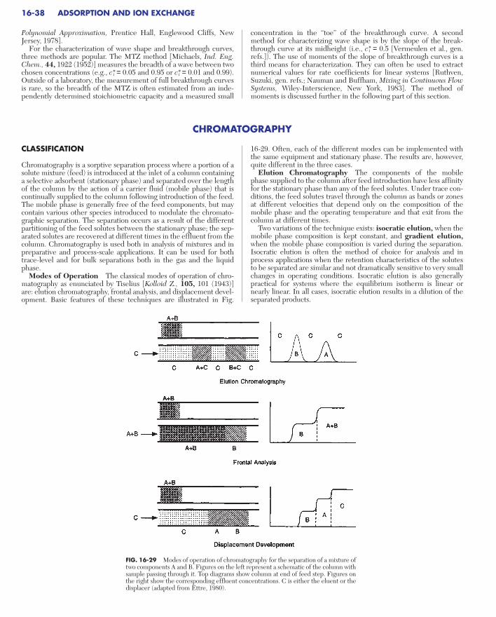
Polynomial Approximation, Prentice Hall, Englewood Cliffs, NewJersey, 1978].
For the characterization of wave shape and breakthrough curves,three methods are popular. The MTZ method [Michaels, Ind. Eng.Chem., 44, 1922 (1952)] measures the breadth of a wave between twochosen concentrations (e.g., c*i = 0.05 and 0.95 or c*i = 0.01 and 0.99).Outside of a laboratory, the measurement of full breakthrough curvesis rare, so the breadth of the MTZ is often estimated from an inde-pendently determined stoichiometric capacity and a measured small
concentration in the “toe” of the breakthrough curve. A secondmethod for characterizing wave shape is by the slope of the break-through curve at its midheight (i.e., c*i = 0.5 [Vermeulen et al., gen.refs.]). The use of moments of the slope of breakthrough curves is athird means for characterization. They can often be used to extractnumerical values for rate coefficients for linear systems [Ruthven,Suzuki, gen. refs.; Nauman and Buffham, Mixing in Continuous FlowSystems, Wiley-Interscience, New York, 1983]. The method ofmoments is discussed further in the following part of this section.
CLASSIFICATION
Chromatography is a sorptive separation process where a portion of asolute mixture (feed) is introduced at the inlet of a column containinga selective adsorbent (stationary phase) and separated over the lengthof the column by the action of a carrier fluid (mobile phase) that iscontinually supplied to the column following introduction of the feed.The mobile phase is generally free of the feed components, but maycontain various other species introduced to modulate the chromato-graphic separation. The separation occurs as a result of the differentpartitioning of the feed solutes between the stationary phase; the sep-arated solutes are recovered at different times in the effluent from thecolumn. Chromatography is used both in analysis of mixtures and inpreparative and process-scale applications. It can be used for bothtrace-level and for bulk separations both in the gas and the liquidphase.
Modes of Operation The classical modes of operation of chro-matography as enunciated by Tiselius [Kolloid Z., 105, 101 (1943)]are: elution chromatography, frontal analysis, and displacement devel-opment. Basic features of these techniques are illustrated in Fig.
16-29. Often, each of the different modes can be implemented withthe same equipment and stationary phase. The results are, however,quite different in the three cases.
Elution Chromatography The components of the mobilephase supplied to the column after feed introduction have less affinityfor the stationary phase than any of the feed solutes. Under trace con-ditions, the feed solutes travel through the column as bands or zonesat different velocities that depend only on the composition of themobile phase and the operating temperature and that exit from thecolumn at different times.
Two variations of the technique exists: isocratic elution, when themobile phase composition is kept constant, and gradient elution,when the mobile phase composition is varied during the separation.Isocratic elution is often the method of choice for analysis and inprocess applications when the retention characteristics of the solutesto be separated are similar and not dramatically sensitive to very smallchanges in operating conditions. Isocratic elution is also generallypractical for systems where the equilibrium isotherm is linear ornearly linear. In all cases, isocratic elution results in a dilution of theseparated products.
16-38 ADSORPTION AND ION EXCHANGE
CHROMATOGRAPHY
FIG. 16-29 Modes of operation of chromatography for the separation of a mixture oftwo components A and B. Figures on the left represent a schematic of the column withsample passing through it. Top diagrams show column at end of feed step. Figures onthe right show the corresponding effluent concentrations. C is either the eluent or thedisplacer (adapted from Ettre, 1980).
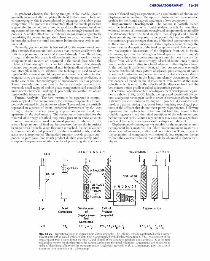
In gradient elution, the eluting strength of the mobile phase isgradually increased after supplying the feed to the column. In liquidchromatography, this is accomplished by changing the mobile phasecomposition. The gradient in eluting strength of the mobile phase thatis generated in the column is used to modulate the separation allow-ing control of the retention time of weakly and strongly retained com-ponents. A similar effect can be obtained in gas chromatography bymodulating the column temperature. In either case, the column has tobe brought back to the initial conditions before the next cycle is com-menced.
Generally, gradient elution is best suited for the separation of com-plex mixtures that contain both species that interact weakly with thestationary phase and species that interact strongly. Since the elutingstrength of the mobile phase is adjusted continuously, weakly retainedcomponents of a mixture are separated in the initial phase when therelative elution strength of the mobile phase is low, while stronglyretained components are separated later in the gradient when the elu-tion strength is high. In addition, the technique is used to obtainreproducible chromatographic separations when the solute retentioncharacteristics are extremely sensitive to the operating conditions, asin the case of the chromatography of biopolymers, such as proteins.These molecules are often found to be very strongly retained in anextremely small range of mobile phase compositions and completelyunretained elsewhere, making it practically impossible to obtainreproducible isocratic separations.
Frontal Analysis The feed mixture to be separated is continu-ously supplied to the column where the mixture components are com-petitively retained by the stationary phase. These solutes are partiallyseparated in a series of fronts, preceded downstream by the leaststrongly retained species forming a pure component band, andupstream by the feed mixture. The technique is best suited for theremoval of strongly adsorbed impurities present in trace amountsfrom an unretained or weakly retained product of interest. In thiscase, a large amount of feed can be processed before the impuritiesbegin to break through. When this point is reached, the bed is washedto remove any desired product from the interstitial voids, and theadsorbent is regenerated. The method can only provide a single com-ponent in pure form, but avoids product dilution completely. Multi-component separations require a series of processing steps; either a
series of frontal analysis separations, or a combination of elution anddisplacement separations. Example 10 illustrates bed concentrationprofiles for the frontal analysis separation of two components.
Displacement Development The column is partially loadedwith the feed mixture as in frontal analysis, usually for conditionswhere all solutes of interest are strongly and competitively retained bythe stationary phase. The feed supply is then stopped and a mobilephase containing the displacer, a component that has an affinity forthe stationary phase stronger than any of the feed components, is fedto the column. The advancement of the displacer front through thecolumn causes desorption of the feed components and their competi-tive readsorption downstream of the displacer front. As in frontalchromatography, the less strongly retained species tends to migratefaster down the column concentrating in a band farthest from the dis-placer front, while the most strongly adsorbed solute tends to movemore slowly concentrating in a band adjacent to the displacer front. If the column is sufficiently long, all feed components eventuallybecome distributed into a pattern of adjacent pure component bandswhere each upstream component acts as a displacer for each down-stream species located in the band immediately downstream. Whenthis occurs, all bands in the displacement train move at the samevelocity which is equal to the velocity of the displacer front and thebed concentration profile is called an isotachic pattern.
The various operational steps of a displacement development separa-tion are shown in Fig. 16-30. Ideally, the separated species exit the col-umn as adjacent rectangular bands in order of increasing affinity for thestationary phase as shown in this figure. In practice, dispersion effectsresult in a partial mixing of adjacent bands requiring recycling of por-tions of the effluent that do not meet purity requirements. Followingseparation, the displacer has to be removed from the column with asuitable regenerant and the initial conditions of the column restoredbefore the next cycle. Column regeneration may consume a significantportion of the cycle, when removal of the displacer is difficult.
Displacement chromatography is suitable for the separation of mul-ticomponent bulk mixtures. For dilute multicomponent mixtures itallows a simultaneous separation and concentration. Thus, it permitsthe separation of compounds with extremely low separation factorswithout the excessive dilution that would be obtained in elution tech-niques.
CHROMATOGRAPHY 16-39
FIG. 16-30 Operational steps in displacement chromatography. The column, initially equilibrated with a carriersolvent at time 0, is loaded with feed until time tF and supplied with displacer for a time tD + tE. Development of thedisplacement train occurs during the time tD and elution of the separated products ends at time tE. tR is the timerequired to remove the displacer from the column and restore the initial conditions. Components are numbered inorder of decreasing affinity for the stationary phase. [Reference: Horvath et al., J. Chromatogr., 218, 365 (1981).Reprinted with permission of J. Chromatogr.]

Other modes of operation, including recycle and flow reversalschemes and continuous chromatography, are discussed in Ganetsosand Barker (Preparative and Production Scale Chromatography,Marcel Dekker, New York, 1993).
CHARACTERIZATION OF EXPERIMENTALCHROMATOGRAMS
Method of Moments The first step in the analysis of chromato-graphic systems is often a characterization of the column response tosmall pulse injections of a solute under trace conditions in the Henry’slaw limit. For such conditions, the statistical moments of the responsepeak are used to characterize the chromatographic behavior. Such anapproach is generally preferable to other descriptions of peak proper-ties which are specific to Gaussian behavior, since the statisticalmoments are directly correlated to equilibrium and dispersion para-meters. Useful references are Schneider and Smith [AIChE J., 14,762 (1968)], Suzuki and Smith [Chem. Eng. Sci., 26, 221 (1971)], andCarbonell et al. [Chem. Eng. Sci., 9, 115 (1975); 16, 221 (1978)].
The relevant moments are:
µ0 = ∞
0ci dt (16-153)
µ1 = ∞
0cit dt (16-154)
σ2 = ∞
0ci(t − µ1)2 dt (16-155)
where ci is the peak profile. µ0 represents the area, µ1 the mean resi-dence time, and σ2 the variance of the response peak. Moments canbe calculated by numerical integration of experimental profiles.
The retention factor is defined as a dimensionless peak locator as:
k′i = (16-156)
where µ10 is the first moment obtained for an inert tracer which is
excluded from the stationary phase. k′i is a partition ratio represent-ing the equilibrium ratio of the amount of solute in the stationaryphase (including any pores) and the amount in the external mobilephase. Another commonly used definition of the retention factoruses as a reference the first moment of an inert that has access to allthe pores.
µ1 − µ10
µ1
0
1µ0
1µ0
The number of plates, Np, and the height equivalent to a theoreticalplate, HETP, are defined as measures of dispersion effects as:
Np = = (16-157)
HETP = (16-158)
A high number of plates and a low HETP indicate a high column effi-ciency.
Higher moments can also be computed and used to define theskewness of the response peak. However, difficulties often arise insuch computations as a result of drifting of the detection system.
In practice, experimental peaks can be affected by extracolumnretention and dispersion factors associated with the injector, connec-tions, and any detector. For linear chromatography conditions, theapparent response parameters are related to their corresponding truecolumn value by
µ1app = µ1 + µ1
inj + µ1conn + µ1
det (16-159)
σ2app = σ2 + σ2inj + σ2conn + σ2det (16-160)
Approximate Methods For certain conditions, symmetrical,Gaussian-like peaks are obtained experimentally. Such peaks may beempirically described by:
ci = exp − 2
= exp − − 12
(16-161)
where Qi is the amount of solute injected, Fv is the volumetric flowrate, and tRi is the peak apex time. The relationships between themoments and other properties of such peaks are shown in Fig. 16-31.For such peaks, approximate calculations of the number of plates canbe done with the following equations:
Np = 5.54 2
(16-162)
Np = 16 2
(16-163)
Np = 2π 2
(16-164)c i
max tRi
µ0
tRiW
tRi∆
ttRi
Np2
Np2π
Qi /Fv
tRi
t − tRiσ2
Qi /Fvσ2π
σ2Lµ1
2
µ12
σ2
LHETP
16-40 ADSORPTION AND ION EXCHANGE
FIG. 16-31 Properties of a Gaussian peak. cimax is the peak height; tRi, the peak apex time; σ, the
standard deviation; ∆, the peak width at midheight; and W, the distance between the baselineintercepts of the tangents to the peak.

where ∆ is the peak width at half peak height and W is the distancebetween the baseline intercepts of the tangents to the inflectionpoints of the peak.
In general, Gaussian behavior can be tested by plotting the cumu-lative fractional recovery t
0 ci dt/µ0 versus time on probability-linearcoordinates; if the plot is linear, Gaussian behavior is confirmed. Fornearly Gaussian peaks, calculations of Np based on Eqs. (16-162) to(16-164) provide results close to those obtained with a rigorous calcu-lation of moments. When deviations from Gaussian behavior are significant, however, large errors can be obtained using these expres-sions.
Tailing Peaks Tailing peaks can be obtained experimentallywhen the column efficiency is very low, when there are large extracol-umn dispersion effects, when the stationary phase is heterogeneous(in the sense that it contains different adsorption sites), or when theadsorption equilibrium deviates from the Henry’s law limit. Asymmet-rical tailing peaks can some times be described empirically by an expo-nentially modified Gaussian (EMG) defined as the convolute integralof a Gaussian constituent with mean time tG and standard deviation σG and an exponential decay with time constant τG [Grushka, Anal.Chem., 44, 1733 (1972)]:
ci = ∞
0exp −
2
− dt′ (16-165)
Although a numerical integration is required to compute the peakprofile, the moments are calculated directly as µ1 = tG + τG and σ2 =σG
2 + τG2 and the peak skew as:
Peak skew = ∞
0ci(t − µ1)3 dt ∼ (16-166)
For EMG peaks, peak skew increases with the ratio τG /σG. Figure 16-32 illustrates the characteristics of such a peak calculated for τG /σG = 1.5. In general, with τG /σG > 1 (peak skew > 0.7), a direct cal-culation of the moments is required to obtained a good approximationof the true value of Np, since other methods give a large error (Yau etal., Moderns Size-Exclusion Liquid Chromatography, Wiley, NewYork, 1979). Alternatively, Eq. (16-165) can be fitted to experimentalpeaks to determine the optimum values of tG, σG, and τG.
In practice, the calculation of peak skew for highly tailing peaks isrendered difficult by baseline errors in the calculation of thirdmoments. The peak asymmetry factor, As = b/a, at 10 percent ofpeak height (see Fig. 16-32) is thus frequently used. An approximaterelationship between peak skew and As for tailing peaks, based on datain Yau et al. is: Peak skew = [0.51 + 0.19/(As − 1)]−1. Values of As < 1.25
2(τG /σG)3
[1 + (τG /σG)2]3/2
1µ0σ3
t′τG
t − tG − t′
σG2Qi /FvσGτG2π
(corresponding to peak skew < 0.7) are generally desirable for an effi-cient chromatographic separation.
Resolution The chromatographic separation of two components,A and B, under trace conditions with small feed injections can becharacterized in terms of the resolution, Rs. For nearly Gaussianpeaks:
Rs = ∼ (16-167)
where ∆tR is the difference in retention time of the two peaks and σAB = (σA + σB)/2 is the average of their standard deviations. When Eq.(16-161) is applicable, the resolution for two closely spaced peaks isapproximated by:
Rs = Np
∼ Np, for α ∼ 1 (16-168)
where α = k′A /k′B and k′ = (k′A + k′B)/2.Equation (16-168) shows that the resolution is the result of inde-
pendent effects of the separation selectivity (α), column efficiency(Np), and capacity (k′). Generally, peaks are essentially completelyresolved when Rs = 1.5 (>99.5 percent separation). In practice, valuesof Rs ∼ 1, corresponding to 98 percent separation, are often consid-ered adequate.
The preceding equations are accurate to within about 10 percentfor feed injections that do not exceed 40 percent of the final peakwidth. For large, rectangular feed injections, the baseline width of theresponse peak is approximated by:
W ∼ 4σ + tF (16-169)
where 4σ is the baseline width obtained with a small pulse injectionand tF is the duration of feed injection. In this case, the resolution isdefined as (see Ruthven, gen. refs., pp. 324–331):
Rs = (16-170)
For strongly retained components (k′ >> 1), the number of platesrequired to obtain a given resolution with a finite feed injection isapproximated by:
Np = 4Rs2
2
1 + 2
(16-171)tF
4σABRs
α + 1α − 1
tR, A − tR, B − tF
4σAB
k′A1 + k′A
α − 1
4
k′i1 + k′i
α − 1α + 1
12
∆tR4σAB
2(tR, A − tR, B)
WA + WB
CHROMATOGRAPHY 16-41
FIG. 16-32 Exponentially modified Gaussian peak with τG /σG = 1.5. The graph also shows thedefinition of the peak asymmetry factor As at 10 percent of peak height.

PREDICTION OF CHROMATOGRAPHIC BEHAVIOR
The conservation equations and the rate models described in the“Rate and Dispersion Factors” can normally be used for a quantitativedescription of chromatographic separations. Alternatively, platemodels can be used for an approximate prediction, lumping togetherall dispersion contributions into a single parameter, the HETP or thenumber of plates [Sherwood et al., Mass Transfer, McGraw-Hill, NewYork, 1975, p. 576; Dondi and Guiochon, Theoretical Advancementsin Chromatography and Related Techniques, NATO-ASI, Series C:Mathematical and Physical Sciences, vol. 383, Kluwer, Dordrecht,1992, pp. 1–61]. Exact analytic solutions are generally available for lin-ear isocratic elution under trace conditions (see Dondi and Guiochon,ibid., Ruthven [gen. refs., pp. 324–335], Suzuki [gen. refs., pp. 224–243]). Other cases generally require numerical solution (see Guio-chon et al., gen. refs.) or approximate treatments with simplified ratemodels.
Isocratic Elution In the simplest case, feed with concentrationc i
F is applied to the column for a time tF followed by the pure carrierfluid. Under trace conditions, for a linear isotherm with external mass-transfer control, the linear driving force approximation or reactionkinetics (see Table 16-12), solution of Eq. (16-146) gives the followingexpression for the dimensionless solute concentration at the columnoutlet:
c*i = J(N, Nτ1) − J(N, Nτ′1) (16-172)
where N is the number of transfer units given in Table 16-13 and τ1 =(εvt/L − ε)/[(1 − ε)(ρpKi + εp)] the throughput parameter (see “SquareRoot Spreading for Linear Isotherms” in “Fixed Bed Transitions”). τ′1represents the value of τ1 with time measured from the end of thefeed step. Thus, the column effluent profile is obtained as the differ-ence between a breakthrough profile for a feed started at t = 0 andanother for a feed started at t = tF.
The behavior predicted by this equation is illustrated in Fig. 16-33with N = 80. τF = (εvtF /L)/[(1 − ε)(ρpKi + εp)] is the dimensionlessduration of the feed step and is equal to the amount of solute fed tothe column divided by the sorption capacity. Thus, at τF = 1, the col-umn has been supplied with an amount of solute equal to the station-ary phase capacity. The graph shows the transition from a case wherecomplete saturation of the bed occurs before elution (τF = 1) to incom-plete saturation as τF is progressively reduced. The lower curves withτF ≤ 0.4 are seen to be nearly Gaussian and centered at a dimension-less time τm ∼ (1 − τF /2). Thus, as τF → 0, the response curveapproaches a Gaussian centered at τ1 = 1.
When τF is small (<<0.4), the solution for a feed pulse representedby a Dirac’s delta function at ζ = 0 can be used in lieu of Eq. (16-172).In terms of the dimensionless concentration c*i = ci /ci
F (Sherwood etal., ibid., pp. 571–577):
c*i = e−Ne−Nτ1I1(2N τ1) (16-173)
where I1 is the Bessel function of imaginary argument. When N islarger than 5, this equation is approximated by:
c*i = (16-174)
The behavior predicted by Eq. (16-174) is shown in Fig. 16-34 asc*i /(τFN) versus τ1 for different values of N. For N > 50, the responsepeak is symmetrical, the peak apex occurs at τ1 = 1, and the dimen-sionless peak height is c*i max = τF N/4π. A comparison of this equationwith Eq. (16-172) with N = 80 is shown in Fig. 16-33 for τF = 0.05.
The moments of the response peak predicted by Eq. (16-173) are
µ1 = 1 + (εp + ρpKi) = (1 + k′i) (16-175)
σ2 = 2
(16-176)
where k′i = (1 − ε)(εp + ρpKi)/ε. Correspondingly, the number of platesand the HETP are:
Np = 2
(16-177)
HETP = 2
(16-178)
Since the term (1 + k′i )/k′i approaches unity for large k′-value, thenumber of plates is equal to one half the number of transfer units fora strongly retained component. For these conditions, when Np = N/2,Eq. (16-174) and Eq. (16-161) produce the same peak retention time,peak spreading, and predict essentially the same peak profile.
In the general case of axially dispersed plug flow with bidispersedparticles, the first and second moment of the pulse response are[Haynes and Sarma, AIChE J., 19, 1043 (1973)]:
µ1 = 1 + (εp + ρpKi) = (1 + k′i) (16-179)Lv
1 − ε
εLv
k′i1 + k′i
2LN
1 + k′i
k′iN2
k′i1 + k′i
2µ12
N
Lv
1 − ε
εLv
exp [−N(τ1 − 1)2]
(τ1)1/4
Nτ1
τF2π
τF Nτ1
16-42 ADSORPTION AND ION EXCHANGE
FIG. 16-33 Elution curves under trace linear equilibrium conditions for different feed loadingperiods and N = 80. Solid lines, Eq. (16-172); dashed line, Eq. (16-174) for τF = 0.05.
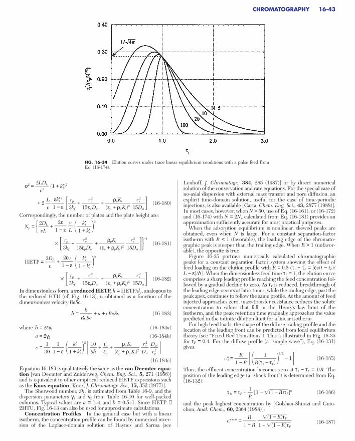
σ2 = (1 + k′i)2
+ 2 + + (16-180)
Correspondingly, the number of plates and the plate height are:
Np = + 2
+ + −1
(16-181)
HETP = + 2
+ + (16-182)
In dimensionless form, a reduced HETP, h = HETP/dp, analogous tothe reduced HTU (cf. Fig. 16-13), is obtained as a function of thedimensionless velocity ReSc:
h = + a + cReSc (16-183)
where b = 2εγ1 (16-184a)
a = 2γ2 (16-184b)
c = 2
+ + (16-184c)
Equation 16-183 is qualitatively the same as the van Deemter equa-tion [van Deemter and Zuiderweg, Chem. Eng. Sci., 5, 271 (1956)]and is equivalent to other empirical reduced HETP expressions suchas the Knox equation [Knox, J. Chromatogr. Sci., 15, 352 (1977)].
The Sherwood number, Sh, is estimated from Table 16-9, and thedispersion parameters γ1 and γ2 from Table 16-10 for well-packedcolumns. Typical values are a = 1–4 and b = 0.5–1. Since HETP ∼2HTU, Fig. 16-13 can also be used for approximate calculations.
Concentration Profiles In the general case but with a linearisotherm, the concentration profile can be found by numerical inver-sion of the Laplace-domain solution of Haynes and Sarma [see
Dpir 2
p
r 2s
Dsi
ρpKi(εp + ρpKi)2
τpεp
10Sh
k′i1 + k′i
11 − ε
130
bReSc
r 2s
15Dsi
ρpKi(εp + ρpKi)2
r 2p
15εpDpi
rp3kf
k′i1 + k′i
2εv1 − ε
2DL
v
r 2s
15Dsi
ρpKi(εp + ρpKi)2
r 2p
15εpDpi
rp3kf
k′i1 + k′i
vL
2ε1 − ε
2DLvL
r 2s
15Dsi
ρpKi(εp + ρpKi)2
r 2p
15εpDpi
rp3kf
εk′i 2
1 − ε
Lv
2LDL
v3
Lenhoff, J. Chromatogr., 384, 285 (1987)] or by direct numericalsolution of the conservation and rate equations. For the special case ofno-axial dispersion with external mass transfer and pore diffusion, anexplicit time-domain solution, useful for the case of time-periodicinjections, is also available [Carta, Chem. Eng. Sci., 43, 2877 (1988)].In most cases, however, when N > 50, use of Eq. (16-161), or (16-172)and (16-174) with N = 2Np calculated from Eq. (16-181) provides anapproximation sufficiently accurate for most practical purposes.
When the adsorption equilibrium is nonlinear, skewed peaks areobtained, even when N is large. For a constant separation-factorisotherm with R < 1 (favorable), the leading edge of the chromato-graphic peak is steeper than the trailing edge. When R > 1 (unfavor-able), the opposite is true.
Figure 16-35 portrays numerically calculated chromatographicpeaks for a constant separation factor system showing the effect offeed loading on the elution profile with R = 0.5 (τ1 − τF = [εv(t − tF)/L − ε]/Λ). When the dimensionless feed time τF = 1, the elution curvecomprises a sharp leading profile reaching the feed concentration fol-lowed by a gradual decline to zero. As τF is reduced, breakthrough ofthe leading edge occurs at later times, while the trailing edge, past thepeak apex, continues to follow the same profile. As the amount of feedinjected approaches zero, mass-transfer resistance reduces the soluteconcentration to values that fall in the Henry’s law limit of theisotherm, and the peak retention time gradually approaches the valuepredicted in the infinite dilution limit for a linear isotherm.
For high feed loads, the shape of the diffuse trailing profile and thelocation of the leading front can be predicted from local equilibriumtheory (see “Fixed Bed Transitions”). This is illustrated in Fig. 16-35for τF = 0.4. For the diffuse profile (a “simple wave”), Eq. (16-131)gives:
c*i = 1/ 2
− 1 (16-185)
Thus, the effluent concentration becomes zero at τ1 − τF = 1/R. Theposition of the leading edge (a “shock front”) is determined from Eq.(16-132):
τ1s = τF + [1 − (1 − R)τF]2 (16-186)
and the peak highest concentration by [Golshan-Shirazi and Guio-chon, Anal. Chem., 60, 2364 (1988)]:
c*i max = (16-187)(1 − R)τF
1 − (1 − R)τF
R1 − R
1R
1R(τ1 − τF)
R1 − R
CHROMATOGRAPHY 16-43
FIG. 16-34 Elution curves under trace linear equilibrium conditions with a pulse feed fromEq. (16-174).
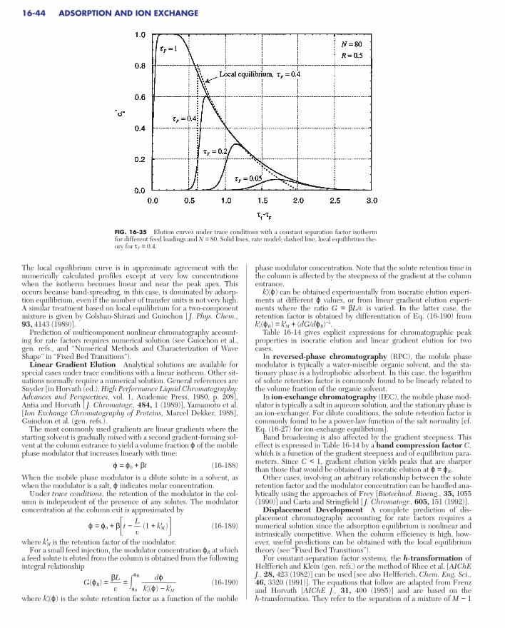
The local equilibrium curve is in approximate agreement with thenumerically calculated profiles except at very low concentrationswhen the isotherm becomes linear and near the peak apex. Thisoccurs because band-spreading, in this case, is dominated by adsorp-tion equilibrium, even if the number of transfer units is not very high.A similar treatment based on local equilibrium for a two-componentmixture is given by Golshan-Shirazi and Guiochon [ J. Phys. Chem.,93, 4143 (1989)].
Prediction of multicomponent nonlinear chromatography account-ing for rate factors requires numerical solution (see Guiochon et al.,gen. refs., and “Numerical Methods and Characterization of WaveShape” in “Fixed Bed Transitions”).
Linear Gradient Elution Analytical solutions are available forspecial cases under trace conditions with a linear isotherm. Other sit-uations normally require a numerical solution. General references areSnyder [in Horvath (ed.), High Performance Liquid Chromatography:Advances and Perspectives, vol. 1, Academic Press, 1980, p. 208],Antia and Horvath [ J. Chromatogr., 484, 1 (1989)], Yamamoto et al.[Ion Exchange Chromatography of Proteins, Marcel Dekker, 1988],Guiochon et al. (gen. refs.).
The most commonly used gradients are linear gradients where thestarting solvent is gradually mixed with a second gradient-forming sol-vent at the column entrance to yield a volume fraction ϕ of the mobilephase modulator that increases linearly with time:
ϕ = ϕ0 + βt (16-188)
When the mobile phase modulator is a dilute solute in a solvent, aswhen the modulator is a salt, ϕ indicates molar concentration.
Under trace conditions, the retention of the modulator in the col-umn is independent of the presence of any solutes. The modulatorconcentration at the column exit is approximated by
ϕ = ϕ0 + βt − (1 + k′M ) (16-189)
where k′M is the retention factor of the modulator.For a small feed injection, the modulator concentration ϕR at which
a feed solute is eluted from the column is obtained from the followingintegral relationship
G(ϕR) = = ϕR
ϕ0
(16-190)
where k′i(ϕ) is the solute retention factor as a function of the mobile
dϕk′i(ϕ) − k′M
βLv
Lv
phase modulator concentration. Note that the solute retention time inthe column is affected by the steepness of the gradient at the columnentrance.
k′i(ϕ) can be obtained experimentally from isocratic elution experi-ments at different ϕ values, or from linear gradient elution experi-ments where the ratio G = βL/v is varied. In the latter case, theretention factor is obtained by differentiation of Eq. (16-190) fromk′i(ϕR) = k′M + (dG/dϕR)−1.
Table 16-14 gives explicit expressions for chromatographic peakproperties in isocratic elution and linear gradient elution for twocases.
In reversed-phase chromatography (RPC), the mobile phasemodulator is typically a water-miscible organic solvent, and the sta-tionary phase is a hydrophobic adsorbent. In this case, the logarithmof solute retention factor is commonly found to be linearly related tothe volume fraction of the organic solvent.
In ion-exchange chromatography (IEC), the mobile phase mod-ulator is typically a salt in aqueous solution, and the stationary phase isan ion-exchanger. For dilute conditions, the solute retention factor iscommonly found to be a power-law function of the salt normality [cf.Eq. (16-27) for ion-exchange equilibrium].
Band broadening is also affected by the gradient steepness. Thiseffect is expressed in Table 16-14 by a band compression factor C,which is a function of the gradient steepness and of equilibrium para-meters. Since C < 1, gradient elution yields peaks that are sharperthan those that would be obtained in isocratic elution at ϕ = ϕR.
Other cases, involving an arbitrary relationship between the soluteretention factor and the modulator concentration can be handled ana-lytically using the approaches of Frey [Biotechnol. Bioeng., 35, 1055(1990)] and Carta and Stringfield [ J. Chromatogr., 605, 151 (1992)].
Displacement Development A complete prediction of dis-placement chromatography accounting for rate factors requires anumerical solution since the adsorption equilibrium is nonlinear andintrinsically competitive. When the column efficiency is high, how-ever, useful predictions can be obtained with the local equilibriumtheory (see “Fixed Bed Transitions”).
For constant-separation factor systems, the h-transformation ofHelfferich and Klein (gen. refs.) or the method of Rhee et al. [AIChEJ., 28, 423 (1982)] can be used [see also Helfferich, Chem. Eng. Sci.,46, 3320 (1991)]. The equations that follow are adapted from Frenzand Horvath [AIChE J., 31, 400 (1985)] and are based on the h-transformation. They refer to the separation of a mixture of M − 1
16-44 ADSORPTION AND ION EXCHANGE
FIG. 16-35 Elution curves under trace conditions with a constant separation factor isothermfor different feed loadings and N = 80. Solid lines, rate model; dashed line, local equilibrium the-ory for τF = 0.4.
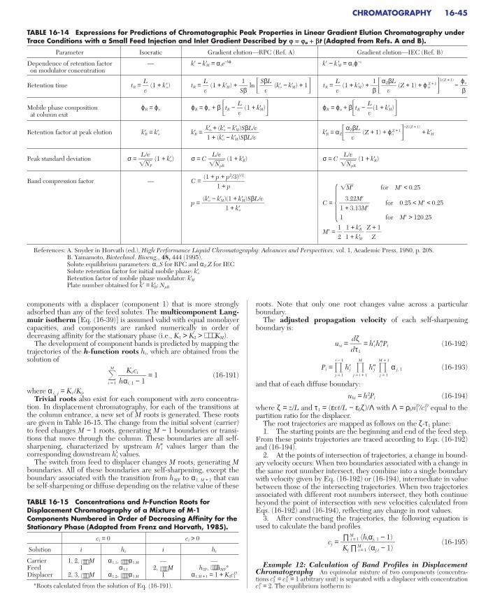
components with a displacer (component 1) that is more stronglyadsorbed than any of the feed solutes. The multicomponent Lang-muir isotherm [Eq. (16-39)] is assumed valid with equal monolayercapacities, and components are ranked numerically in order ofdecreasing affinity for the stationary phase (i.e., K1 > K2 > ⋅ ⋅ ⋅ KM).
The development of component bands is predicted by mapping thetrajectories of the h-function roots hi, which are obtained from thesolution of
M
i = 1
= 1 (16-191)
where α i, j = K i /Kj.Trivial roots also exist for each component with zero concentra-
tion. In displacement chromatography, for each of the transitions atthe column entrance, a new set of M roots is generated. These rootsare given in Table 16-15. The change from the initial solvent (carrier)to feed changes M − 1 roots, generating M − 1 boundaries or transi-tions that move through the column. These boundaries are all self-sharpening, characterized by upstream h″i values larger than thecorresponding downstream h′i values.
The switch from feed to displacer changes M roots, generating Mboundaries. All of these boundaries are self-sharpening, except theboundary associated with the transition from hMF to α1, M + 1 that canbe self-sharpening or diffuse depending on the relative value of these
Kicihα i, 1 − 1
roots. Note that only one root changes value across a particularboundary.
The adjusted propagation velocity of each self-sharpeningboundary is:
usi = = h′ih″i Pi (16-192)
Pi = i − 1
j = 1
h′j M
j = i + 1
h″j M + 1
j = 1
α j, 1 (16-193)
and that of each diffuse boundary:
uhi = h i2Pi (16-194)
where ζ = z/L and τ1 = (εvt/L − εbζ)/Λ with Λ = ρbn1D/c1
D equal to thepartition ratio for the displacer.
The root trajectories are mapped as follows on the ζ-τ1 plane:1. The starting points are the beginning and end of the feed step.
From these points trajectories are traced according to Eqs. (16-192)and (16-194).
2. At the points of intersection of trajectories, a change in bound-ary velocity occurs: When two boundaries associated with a change inthe same root number intersect, they combine into a single boundarywith velocity given by Eq. (16-192) or (16-194), intermediate in valuebetween those of the intersecting trajectories. When two trajectoriesassociated with different root numbers intersect, they both continuebeyond the point of intersection with new velocities calculated fromEqs. (16-192) and (16-194), reflecting any change in root values.
3. After constructing the trajectories, the following equation isused to calculate the band profiles
cj = (16-195)
Example 12: Calculation of Band Profiles in DisplacementChromatography An equimolar mixture of two components (concentra-tions c2
F = c3F = 1 arbitrary unit) is separated with a displacer with concentration
c1F = 2. The equilibrium isotherm is:
∏Mi = 1 (hiα j, 1 − 1)
Kj ∏M
i = 1 (α j,i − 1)
dζdτ1
CHROMATOGRAPHY 16-45
TABLE 16-14 Expressions for Predictions of Chromatographic Peak Properties in Linear Gradient Elution Chromatography underTrace Conditions with a Small Feed Injection and Inlet Gradient Described by j = jo + bt (Adapted from Refs. A and B).
Parameter Isocratic Gradient elution—RPC (Ref. A) Gradient elution—IEC (Ref. B)
Dependence of retention factor — k′ − k′M = αse−Sϕ k′ − k ′M = αzϕ−z
on modulator concentration
Retention time tR = (1 + k ′o) tR = (1 + k′M) + ln (k′o − k′M) + 1 tR = (1 + k′M) + (Z + 1) + ϕ oZ + 1
1/(Z + 1)
−
Mobile phase composition ϕR = ϕo ϕR = ϕo + β tR − (1 + k′M) ϕR = ϕo + βtR − (1 + k′M)at column exit
Retention factor at peak elution k′R = k′o k′R = k′R = αZ (Z + 1) + ϕoZ + 1
−Z/(Z + 1)
+ k′M
Peak standard deviation σ = (1 + k′o) σ = C (1 + k′R) σ = C (1 + k′R)
Band compression factor — C =M′ for M′ < 0.25
p = C = for 0.25 < M′ < 0.25
1 for M′ > 120.25
M′ =
References: A. Snyder in Horvath (ed.), High Performance Liquid Chromatography: Advances and Perspectives, vol. 1, Academic Press, 1980, p. 208.B. Yamamoto, Biotechnol. Bioeng., 48, 444 (1995).Solute equilibrium parameters: αs,S for RPC and αZ,Z for IECSolute retention factor for initial mobile phase: k′oRetention factor of mobile phase modulator: k′MPlate number obtained for k′ = k′R: NpR
Z + 1
Z1 + k′R1 + k′M
12
3.22M′1 + 3.13M′
(k′o − k′M)(1 + k′M)SβL/v
1 + k′o
(1 + p + p2/3)1/2
1 + p
L/vNpR
L/vNpR
L/vNP
αZβL
vk′o + (k′o − k′M)SβL/v1 + (k′o − k′M)SβL/v
Lv
Lv
ϕoβ
αZβL
v1
β
Lv
SβL
v1
Sβ
Lv
Lv
TABLE 16-15 Concentrations and h-Function Roots forDisplacement Chromatography of a Mixture of M-1Components Numbered in Order of Decreasing Affinity for theStationary Phase (Adapted from Frenz and Horvath, 1985).
ci = 0 ci > 0
Solution i hi i hi
Carrier 1, 2, ⋅⋅⋅⋅ M α1,1, ⋅⋅⋅⋅ α1,M — —Feed 1 α1,1 2, ⋅⋅⋅⋅ M h2F, ⋅⋅⋅⋅hMF*Displacer 2, 3, ⋅⋅⋅⋅ M α1,2, ⋅⋅⋅⋅ α1,M 1 α1,M + 1 = 1 + K1c1
D
*Roots calculated from the solution of Eq. (16-191).
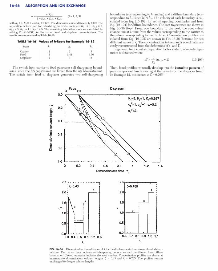
ni = (i = 1, 2, 3)
with K1 = 2, K2 = 1, and K3 = 0.667. The dimensionless feed time is τF = 0.2. Theseparation factors used for calculating the trivial roots are α1, 1 = 1, α1, 2 = 2, α1, 3 = 3, α1, 4 = 1 + K1c1
D = 5. The remaining h-function roots are calculated bysolving Eq. (16-191) for the carrier, feed, and displacer concentrations. Theresults are summarized in Table 16-16.
The switch from carrier to feed generates self-sharpening bound-aries, since the h″is (upstream) are larger than the h′is (downstream).The switch from feed to displacer generates two self-sharpening
nsKici1 + K1c1 + K2c2 + K3c3
boundaries (corresponding to h1 and h2) and a diffuse boundary (cor-responding to h3) since h″3 < h′3 . The velocity of each boundary is cal-culated from Eq. (16-192) for self-sharpening boundaries and fromEq. (16-194) for diffuse boundaries. The root trajectories are shown inFig. 16-36 (top). From one boundary to the next, the root valueschange one at a time from the values corresponding to the carrier tothe values corresponding to the displacer. Concentration profiles cal-culated from Eq. (16-195) are shown in Fig. 16-36 (bottom) for twodifferent values of ζ. The concentrations in the z and t coordinates areeasily reconstructed from the definitions of τ1 and ζ.
In general, for a constant separation factor system, complete sepa-ration is obtained when:
c1D > (α1, M − 1) (16-196)
Then, band profiles eventually develop into the isotachic pattern ofpure component bands moving at the velocity of the displacer front.In Example 12, this occurs at ζ = 0.765.
1K1
16-46 ADSORPTION AND ION EXCHANGE
TABLE 16-16 Values of h-Roots for Example 16-12
State h1 h2 h3
Carrier 1 2 3Feed 1 2.44 6.56Displacer 2 3 5
FIG. 16-36 Dimensionless time-distance plot for the displacement chromatography of a binarymixture. The darker lines indicate self-sharpening boundaries and the thinner lines diffuseboundaries. Circled numerals indicate the root number. Concentration profiles are shown atintermediate dimensionless column lengths ζ = 0.43 and ζ = 0.765. The profiles remainunchanged for longer column lengths.

The isotachic concentrations ciI in the fully developed train are
calculated directly from the single component isotherms using:
= = ⋅ ⋅ ⋅ = (16-197)
or cjI = c1
D − (1 − αj, 1) (16-198)
The graphical interpretation of Eq. (16-197) is shown in Fig. 16-37 forthe conditions of Example 12. An operating line is drawn from the ori-gin to the point of the pure displacer isotherm at c1 = c1
D. For dis-placement to occur, the operating line must cross the pure componentisotherms of the feed solutes. The product concentrations in the iso-tachic train are found where the operating line crosses the isotherms.When this condition is met, the feed concentrations do not affect thefinal product concentrations.
Analyses of displacement chromatography by the method of char-acteristics with non-Langmuirian systems is discussed by Antia andHorvath [ J. Chromatogr., 556, 199 (1991)] and Carta and Dinerman[AIChE J., 40, 1618 (1994)]. Optimization studies and analyses bycomputer simulations are discussed by Jen and Pinto [ J. Chromatogr.,590, 47 (1992)], Katti and Guiochon [ J. Chromatogr., 449, 24(1988)], and Phillips et al. [ J. Chromatogr., 54, 1 (1988)].
DESIGN FOR TRACE SOLUTE SEPARATIONS
The design objectives of the analyst and the production line engineerare generally quite different. For analysis the primary concern is typi-cally resolution. Hence operating conditions near the minimum valueof the HETP or the HTU are desirable (see Fig. 16-13).
In preparative chromatography, however, it is generally desirable toreduce capital costs by maximizing the productivity, or the amount offeed processed per unit column volume, subject to specified purityrequirements. This reduction, however, must be balanced against oper-ating costs that are determined mainly by the mobile phase flow rateand the pressure drop. In practice, preparative chromatography is oftencarried out under overload conditions, i.e., in the nonlinear region ofthe adsorption isotherm. Optimization under these conditions is dis-cussed in Guiochon et al. (gen. refs.). General guidelines for trace-level,isocratic binary separations, in the Henry’s law limit of the isotherm are:
1. The stationary phase is selected to provide the maximum selec-tivity. Where possible, the retention factor is adjusted (by varying themobile phase composition, temperature, or pressure) to an optimumvalue that generally falls between 2 and 10. Resolution is adverselyaffected when k′ << 2, while product dilution and separation time
1Kj
nMe
cM
I
n2e
c2
I
n1e
c1
I
increase greatly when k′ >> 10. When this is not possible for all feedcomponents and large differences exist among the k′-values of the dif-ferent solutes, gradient elution should be considered.
2. The average feed mixture charging rate, molar or volumetric, isfixed by the raw material supply or the demand for finished product.
3. The value of Np required to achieve a desired resolution isdetermined by Eq. (16-168) or (16-171). Since N = L/HTU ∼ 2Np =2L/HETP, Fig. 16-13 or Eq. (16-183) can be used to determine therange of the dimensionless velocity ReSc that maximizes Np for a givenparticle diameter and column length.
4. The allowable pressure drop influences the choice of the parti-cle size and helps determine the column length. Equations for esti-mating the pressure drop in packed beds are given in Section 6.
5. When only a few solutes are separated, they may occupy only asmall portion of the total column volume at any given instant. In suchcases, the productivity is improved by cyclic feed injections, timed sothat the most strongly retained component from an injection elutesjust before the least strongly retained component from the followinginjection (see Fig. 16-57). For a mixture of two components with k′ > 1, when the same resolution is maintained between bands of thesame injections and bands of successive injections, the cycle time tC
and the plate number requirement are:
tC = 2(tR,A − tR,B) = (k′A − k′B) (16-199)
Np = 4Rs2
2
(1 − 2φ)−2 (16-200)
where φ = tF /tC is the fraction of the cycle time during which feed issupplied to the column. The productivity, P = volume of feed/(time ×bed volume), is:
P = 2
φ(1 − 2φ)2
= 2
φ(1 − 2φ)2 (16-201)
For a given resolution, P is maximized when φ =1/6 (i.e., feed is sup-plied for one sixth of the cycle time), and by the use of small particlesizes. The function ReSc/(b/ReSc + a + cReSc) generally increases withReSc, so that productivity generally increases with the mobile phasevelocity. For typical columns, however, this function is within about 10percent of its maximum value (∼ 1/c) when ReSc is in the range30–100. Thus, increasing the velocity above this range must be bal-anced against the costs associated with the higher pressure drop.
ReScb/ReSc + a + cReSc
Didp
2
α − 1α + 1
14Rs
2
εvHETP
α − 1α + 1
14Rs
2
α + 1α − 1
2Lv
CHROMATOGRAPHY 16-47
FIG. 16-37 Schematic showing the intersection of the operating line with the pure-componentisotherms in displacement chromatography. Conditions are the same as in Fig. 16-36.
GENERAL CONCEPTS
Some applications of adsorption and ion exchange can be achieved bysorbent-fluid contact in batch equipment. Batch methods are welladapted to laboratory use and have also been applied on a larger scalein several specific instances. In a batch run for either adsorption or ionexchange, a sorbent is added to a fluid, completely mixed, and subse-quently separated. Batch treatment is adopted when the capacity andequilibrium of the sorbent are large enough to give nearly completesorption in a single step, as in purifying and decoloration of laboratorypreparations with carbons and clays. Batch runs are useful in the mea-surement of equilibrium isotherms and also of adsorptive diffusionrate. Batch tests or measurements are often conducted in portions ofadsorbent or ion-exchange material intended for larger-scale use. Forexample, either the equilibrium sorption of a solid and/or its ultimatesorption capacity can be determined in this way. The solid is firstequilibrated with a fluid at the concentration of interest; after sepa-rating the phases, gravimetric and chemical analyses can be used todetermine the sorbed amount and composition.
Like the laboratory batch use, some commercial applications usethe adsorbent on a throwaway basis. Reasons for using sorption non-regeneratively are usually: (1) low cost of the sorbent, (2) high value ofthe product, (3) very low dosage (sorbent-to-fluid ratio), and (4) diffi-culty in desorbing the sorbates. Magnesium perchlorate and bariumoxide are used for drying, iron sponge (hydrated iron oxide on woodchips) is used to remove hydrogen sulfide, and sodium or potassiumhydroxide is applied to removal of sulfur compounds or carbon diox-ide. In wastewater treatment, powdered activated carbon (PAC) isadded to enhance biological treatment but is not regenerated; instead,it remains with the sludge. Silica gel is used as a desiccant in packag-ing. Activated carbon is used in packaging and storage to adsorb otherchemicals for preventing the tarnishing of silver, retarding the ripen-ing or spoiling of fruits, “gettering” (scavenging) out-gassed solventsfrom electronic components, and removing odors. Synthetic zeolites,or blends of zeolites with silica gel, are used in dual-pane windows toadsorb water during initial dry-down and any in-leakage and to adsorborganic solvents emitted from the sealants during their cure; this pre-vents fogging between the sealed panes that could result from thecondensation of water or the solvents [Ausikaitis, Glass Digest, 61,69–78 (1982)]. Activated carbon is used to treat recirculated air inoffice buildings, apartments, and manufacturing plants using thin fil-ter-like frames to treat the large volumes of air with low pressure drop.On a smaller scale, activated carbon filters are in kitchen hoods, airconditioners, and electronic air purifiers. On the smallest scale, gasmasks containing carbon or carbon impregnated with promoters areused to protect individual wearers from industrial odors, toxic chemi-cals, and gas-warfare chemicals. Activated carbon fibers have beenformed into fabrics for clothing to protect against vesicant and percu-taneous chemical vapors [Macnair and Arons in Cheremisinoff andEllerbusch (eds.), gen. refs.].
Ion exchangers are sometimes used on a throwaway basis also. Inthe laboratory, ion exchangers are used to produce deionized water,purify reagents, and prepare inorganic sols. In medicine, they are usedas antacid, for sodium reduction, for the sustained release of drugs, inskin-care preparations, and in toxin removal.
Although there are many practical applications for which the sor-bent is discarded after one use, most applications of interest to chem-ical engineers involve the removal of adsorbates from the sorbent (i.e.,regeneration). This allows the adsorbent to be reused and the adsor-bates to be recovered.
The maximum efficiency that a cyclic adsorption process canapproach for any given set of operating conditions is defined by theadsorptive loading in equilibrium with the feed fluid. There are sev-eral factors that reduce the practical (or “operating”) adsorption:mass-transfer resistance (see above), deactivation (see above), andincomplete regeneration (or desorption). The severity of regenerationinfluences how closely the dynamic capacity of an adsorbent resem-bles that of fresh, virgin material. Regeneration, or reversal of the
adsorption process, requires a reduction in the driving force foradsorption. This is accomplished by increasing the equilibrium drivingforce for the adsorbed species to desorb from the solid to the sur-rounding fluid.
TEMPERATURE SWING ADSORPTION
A temperature-swing, or thermal-swing, adsorption (TSA) processcycle is one in which desorption takes place at a temperature muchhigher than adsorption. The elevation of temperature is used to shiftthe adsorption equilibrium and affect regeneration of the adsorbent.Figure 16-38 depicts a simplified (and ideal) TSA cycle. The feed fluidcontaining an adsorbate at a partial pressure of p1 is passed through anadsorbent at temperature T1. This adsorption step continues until theequilibrium loading n1 is achieved with p1. Next the adsorbent tem-perature is raised to T2 (heating step) so that the partial pressure inequilibrium with n1 is increased to p2, creating a partial pressure driv-ing force for desorption into any fluid containing less than p2 of theadsorbate. By means of passing a purge fluid across the adsorbent,adsorbate is swept away, and the equilibrium proceeds down theisotherm to some point such as p1, n2. (This point need not coincidewith the feed partial pressure; it is selected for illustrative purposes.Also, in some applications, roll-up of the adsorbed-phase concentra-tion can occur during heating such that in some regions of the bed p2
reaches the condensation pressure of the component, causing a con-densed liquid phase to form temporarily in particles [Friday andLeVan, AIChE J., 31, 1322 (1985)].) During a cooling step, the adsor-bent temperature is returned to T1. The new equilibrium p3, n2 repre-sents the best-quality product that can be produced from theadsorbent at a regenerated loading of n2 in the simplest cycle. Theadsorption step is now repeated. The differential loading, n1 − n2, isthe maximum loading that can be achieved for a TSA cycle operatingbetween a feed containing p1 at temperature T1, regeneration at T2,and a product containing a partial pressure p3 of the adsorbate. Theregeneration fluid will contain an average partial pressure between p2
and p1 and will therefore have accomplished a concentration of theadsorbate in the regenerant fluid. For liquid-phase adsorption, thepartial pressure can be replaced by the fugacity of the adsorbate.Then, the entire discussion above is applicable whether the regenera-tion is by a fluid in the gas or liquid phase.
In a TSA cycle, the heating step must provide the thermal energynecessary to raise the adsorbate, adsorbent, and adsorber tempera-tures, to desorb the adsorbate, and to make up for heat losses. TSAregeneration is classified as (1) heating-limited (or stoichiometric-limited) when transfer of energy to the system is limiting, or (2) strip-ping-limited (or equilibrium-limited) when transferring adsorbateaway is limiting. Heating is accomplished by either direct contact of the adsorbent by the heating medium (external heat exchange to a purge gas) or indirect means (heating elements, coils, or panelsinside the adsorber). Direct heating is the most commonly used, espe-cially for stripping-limited heating. Indirect heating can be consideredfor stripping-limited heating, but the complexity of indirect heatinglimits its practicality to heating-limited regeneration where purge gas is in short supply. Microwave fields [Benchanaa, Lallemant,Simonet-Grange, and Bertrand, Thermochim. Acta, 152, 43–51(1989)] and dielectric fields [Burkholder, Fanslow, and Bluhm, Ind.Eng. Chem. Fundam., 25, 414–416 (1986)] are also used to supplyindirect heating.
Because high temperatures can be used, resulting in thorough de-sorption, TSA cycles are characterized by low residual loadings andthus high operating loadings. These high capacities at low concentra-tions allow long cycle times for reasonably sized adsorbers (hours todays). Long cycle time is needed because particles of adsorbentrespond slowly to changes in gas temperature. Most applications ofTSA are for systems in which adsorbates are present at low concentra-tion (purification), such as drying, and in which species are stronglyadsorbed, such as sweetening, CO2 removal, and pollution control.
16-48 ADSORPTION AND ION EXCHANGE
PROCESS CYCLES
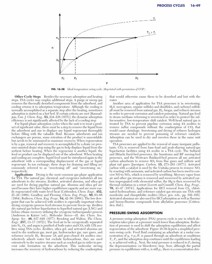
Other Cycle Steps Besides the necessary adsorption and heatingsteps, TSA cycles may employ additional steps. A purge or sweep gasremoves the thermally desorbed components from the adsorbent, andcooling returns it to adsorption temperature. Although the cooling isnormally accomplished as a separate step after the heating, sometimesadsorption is started on a hot bed. If certain criteria are met [Basmad-jian, Can. J. Chem. Eng., 53, 234–238 (1975)], the dynamic adsorptionefficiency is not significantly affected by the lack of a cooling step.
For liquid-phase adsorption cycles when the unit is to treat a prod-uct of significant value, there must be a step to remove the liquid fromthe adsorbent and one to displace any liquid regenerant thoroughlybefore filling with the valuable fluid. Because adsorbents and ionexchangers are porous, some retention of the product is unavoidablebut needs to be minimized to maximize recovery. When regenerationis by a gas, removal and recovery is accomplished by a drain (or pres-sure-assisted drain) step using the gas to help displace liquid from thesorbent before heating. When the regenerant is another liquid, thefeed or product can be displaced out of the adsorbent. When heatingand cooling are complete, liquid feed must be introduced again to theadsorbent with a corresponding displacement of the gas or liquidregenerant. In ion exchange, these steps for draining and filling arecommonly referred to as “sweetening off” and “sweetening on,”respectively.
Applications Drying is the most common gas-phase applicationfor TSA. The natural gas, chemical, and cryogenics industries all useadsorbents to dry streams. Zeolites, activated alumina, and silica gelare used for drying pipeline natural gas. Alumina and silica gel areused because they have higher equilibrium capacity and are more eas-ily regenerated with waste-level heat [Crittenden, Chem. Engr., 452,21–24 (1988); Goodboy and Fleming, Chem. Eng. Progr., 80, 63–68(1984); Ruthven, Chem. Eng. Progr., 84, 42–50 (1988)]. The low dew-point that can be achieved with zeolites is especially important whendrying cryogenic-process feed-streams to prevent freeze-up. Zeolitesdry natural gas before liquefaction to liquefied natural gas (LNG) andbefore ethane recovery utilizing the cryogenic turboexpander process[Anderson in Katzer (ed.), Molecular Sieves—II, Am. Chem. Soc.Symp. Ser., 40, 637–649 (1977); Brooking and Walton, The Chem.Engr., 257, 13–17 (1972)]. The feed air to be cryogenically separatedinto N2, O2, and argon is purified of both water and CO2 with 13X zeo-lites using TSA cycles. Zeolites, silica gel, and activated alumina areused to dry synthesis gas, inert gas, hydrocracker gas, rare gases, andreformer recycle H2. Because 3A and pore-closed 4A zeolites size-selectively adsorb water but exclude hydrocarbons, they are usedextensively to dry reactive streams such as cracked gas in order to pre-vent coke formation on the adsorbent. This molecular sievingincreases the recovery of hydrocarbons by reducing the coadsorption
that would otherwise cause them to be desorbed and lost with thewater.
Another area of application for TSA processes is in sweetening.H2S, mercaptans, organic sulfides and disulfides, and carbonyl sulfideall must be removed from natural gas, H2, biogas, and refinery streamsin order to prevent corrosion and catalyst poisoning. Natural gas feedto steam methane reforming is sweetened in order to protect the sul-fur-sensitive, low-temperature shift catalyst. Well-head natural gas istreated by TSA to prevent pipeline corrosion using 4A zeolites toremove sulfur compounds without the coadsorption of CO2 thatwould cause shrinkage. Sweetening and drying of refinery hydrogenstreams are needed to prevent poisoning of reformer catalysts.Adsorption can be used to dry and sweeten these in the same unitoperation.
TSA processes are applied to the removal of many inorganic pollu-tants. CO2 is removed from base-load and peak-shaving natural-gasliquefaction facilities using 4A zeolite in a TSA cycle. The Sulfacid and Hitachi fixed-bed processes, the Sumitomo and BF moving-bedprocesses, and the Westvaco fluidized-bed process all use activatedcarbon adsorbents to remove SO2 from flue gases and sulfuric acidplant tail gases [Juentgen, Carbon, 15, 273–283 (1977)]. Activatedcarbon with a catalyst is used by the Unitaka process to remove NOx
by reacting with ammonia, and activated carbon has been used to con-vert NO to NO2, which is removed by scrubbing. Mercury vapor fromair and other gas streams is removed and recovered by activated car-bon impregnated with elemental sulfur; the Hg is then recovered bythermal oxidation in a retort [Lovett and Cunniff, Chem. Eng. Progr.,70, 43–47 (1974)]. Applications for HCl removal from Cl2, chlori-nated hydrocarbons, and reformer catalyst gas streams use TSA withmordenite and clinoptilolite zeolites [Dyer, gen. refs., pp. 102–105].Activated aluminas are also used for HCl adsorption as well as fluorineand boron-fluorine compounds from alkylation processes [Critten-den, ibid.].
PRESSURE-SWING ADSORPTION
A pressure-swing adsorption (PSA) process cycle is one in which de-sorption takes place at a pressure much lower than adsorption. Reduc-tion of pressure is used to shift the adsorption equilibrium and affectregeneration of the adsorbent. Figure 16-39 depicts a simplified pres-sure-swing cycle. Feed fluid containing an adsorbate at a molar con-centration of y1 = p1 /P1 is passed through an adsorbent at conditionsT1, P1, and the adsorption step continues until the equilibrium loadingn1 is achieved with y1. Next, the total pressure is reduced to P2 duringthe depressurization (or blowdown) step. Now, although the partialpressure in equilibrium with n1 is still p1, there is a concentration driv-
PROCESS CYCLES 16-49
FIG. 16-38 Ideal temperature swing cycle. (Reprinted with permission of UOP.)
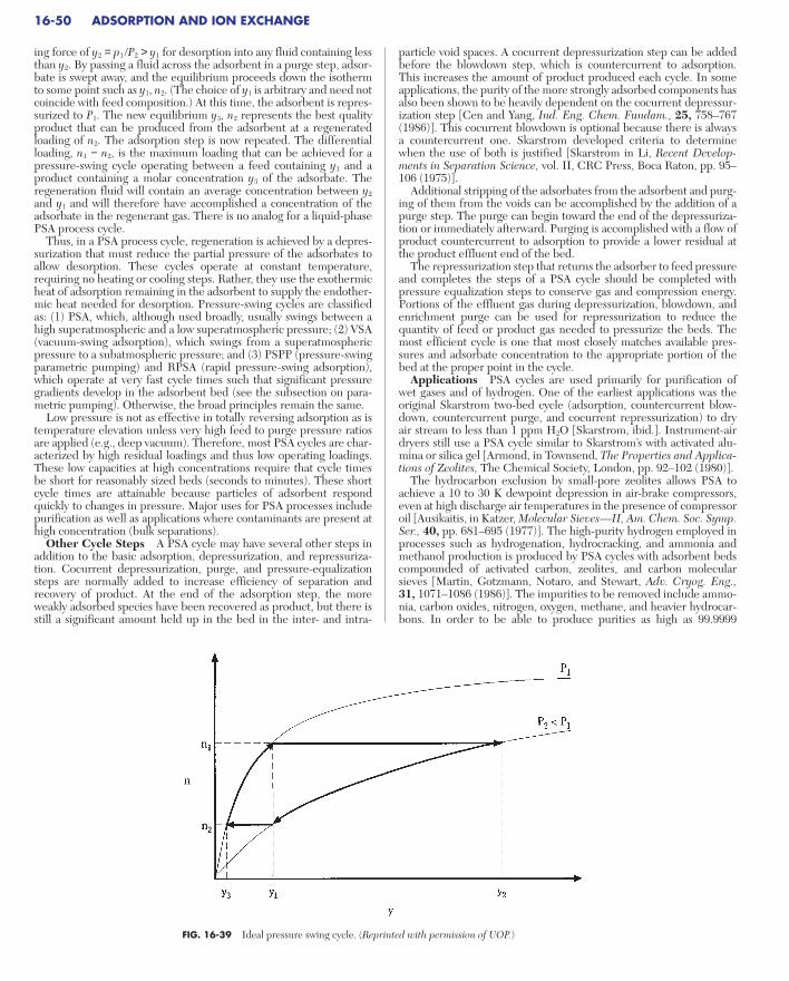
ing force of y2 = p1 /P2 > y1 for desorption into any fluid containing lessthan y2. By passing a fluid across the adsorbent in a purge step, adsor-bate is swept away, and the equilibrium proceeds down the isothermto some point such as y1, n2. (The choice of y1 is arbitrary and need notcoincide with feed composition.) At this time, the adsorbent is repres-surized to P1. The new equilibrium y3, n2 represents the best qualityproduct that can be produced from the adsorbent at a regeneratedloading of n2. The adsorption step is now repeated. The differentialloading, n1 − n2, is the maximum loading that can be achieved for apressure-swing cycle operating between a feed containing y1 and aproduct containing a molar concentration y3 of the adsorbate. Theregeneration fluid will contain an average concentration between y2
and y1 and will therefore have accomplished a concentration of theadsorbate in the regenerant gas. There is no analog for a liquid-phasePSA process cycle.
Thus, in a PSA process cycle, regeneration is achieved by a depres-surization that must reduce the partial pressure of the adsorbates toallow desorption. These cycles operate at constant temperature,requiring no heating or cooling steps. Rather, they use the exothermicheat of adsorption remaining in the adsorbent to supply the endother-mic heat needed for desorption. Pressure-swing cycles are classifiedas: (1) PSA, which, although used broadly, usually swings between ahigh superatmospheric and a low superatmospheric pressure; (2) VSA(vacuum-swing adsorption), which swings from a superatmosphericpressure to a subatmospheric pressure; and (3) PSPP (pressure-swingparametric pumping) and RPSA (rapid pressure-swing adsorption),which operate at very fast cycle times such that significant pressuregradients develop in the adsorbent bed (see the subsection on para-metric pumping). Otherwise, the broad principles remain the same.
Low pressure is not as effective in totally reversing adsorption as istemperature elevation unless very high feed to purge pressure ratiosare applied (e.g., deep vacuum). Therefore, most PSA cycles are char-acterized by high residual loadings and thus low operating loadings.These low capacities at high concentrations require that cycle timesbe short for reasonably sized beds (seconds to minutes). These shortcycle times are attainable because particles of adsorbent respondquickly to changes in pressure. Major uses for PSA processes includepurification as well as applications where contaminants are present athigh concentration (bulk separations).
Other Cycle Steps A PSA cycle may have several other steps inaddition to the basic adsorption, depressurization, and repressuriza-tion. Cocurrent depressurization, purge, and pressure-equalizationsteps are normally added to increase efficiency of separation andrecovery of product. At the end of the adsorption step, the moreweakly adsorbed species have been recovered as product, but there isstill a significant amount held up in the bed in the inter- and intra-
particle void spaces. A cocurrent depressurization step can be addedbefore the blowdown step, which is countercurrent to adsorption.This increases the amount of product produced each cycle. In someapplications, the purity of the more strongly adsorbed components hasalso been shown to be heavily dependent on the cocurrent depressur-ization step [Cen and Yang, Ind. Eng. Chem. Fundam., 25, 758–767(1986)]. This cocurrent blowdown is optional because there is alwaysa countercurrent one. Skarstrom developed criteria to determinewhen the use of both is justified [Skarstrom in Li, Recent Develop-ments in Separation Science, vol. II, CRC Press, Boca Raton, pp. 95–106 (1975)].
Additional stripping of the adsorbates from the adsorbent and purg-ing of them from the voids can be accomplished by the addition of apurge step. The purge can begin toward the end of the depressuriza-tion or immediately afterward. Purging is accomplished with a flow ofproduct countercurrent to adsorption to provide a lower residual atthe product effluent end of the bed.
The repressurization step that returns the adsorber to feed pressureand completes the steps of a PSA cycle should be completed withpressure equalization steps to conserve gas and compression energy.Portions of the effluent gas during depressurization, blowdown, andenrichment purge can be used for repressurization to reduce thequantity of feed or product gas needed to pressurize the beds. Themost efficient cycle is one that most closely matches available pres-sures and adsorbate concentration to the appropriate portion of thebed at the proper point in the cycle.
Applications PSA cycles are used primarily for purification ofwet gases and of hydrogen. One of the earliest applications was theoriginal Skarstrom two-bed cycle (adsorption, countercurrent blow-down, countercurrent purge, and cocurrent repressurization) to dryair stream to less than 1 ppm H2O [Skarstrom, ibid.]. Instrument-airdryers still use a PSA cycle similar to Skarstrom’s with activated alu-mina or silica gel [Armond, in Townsend, The Properties and Applica-tions of Zeolites, The Chemical Society, London, pp. 92–102 (1980)].
The hydrocarbon exclusion by small-pore zeolites allows PSA toachieve a 10 to 30 K dewpoint depression in air-brake compressors,even at high discharge air temperatures in the presence of compressoroil [Ausikaitis, in Katzer, Molecular Sieves—II, Am. Chem. Soc. Symp.Ser., 40, pp. 681–695 (1977)]. The high-purity hydrogen employed inprocesses such as hydrogenation, hydrocracking, and ammonia andmethanol production is produced by PSA cycles with adsorbent bedscompounded of activated carbon, zeolites, and carbon molecularsieves [Martin, Gotzmann, Notaro, and Stewart, Adv. Cryog. Eng.,31, 1071–1086 (1986)]. The impurities to be removed include ammo-nia, carbon oxides, nitrogen, oxygen, methane, and heavier hydrocar-bons. In order to be able to produce purities as high as 99.9999
16-50 ADSORPTION AND ION EXCHANGE
FIG. 16-39 Ideal pressure swing cycle. (Reprinted with permission of UOP.)

percent, systems such as a UOPTM PolybedTM separation unit use six toten adsorbers with complex cycles (see below) [Fuderer and Rudel-storfer, U.S. Patent 3,986,849 (1976)].
Air separation, methane enrichment, and iso/normal separationsare the major bulk separations utilizing PSA; recovery of CO and CO2
are also growing uses. PSA process cycles are used to produce oxygenand/or nitrogen from air. Synthetic zeolites, clinoptilolite, mordenite,and carbon molecular sieves are all used in various PSA, VSA, andRPSA cycles. The 85 to 95 percent purity oxygen produced isemployed for electric furnace steel, waste water treating, solid wastecombustion, and kilns [Martin et al., ibid.]. Small PSA oxygen unitsare used for patients requiring inhalation therapy in the hospital andat home [Cassidy and Holmes, AIChE Symp. Ser., 80 (1984), pp. 68–75] and for pilots on board aircraft [Tedor, Horch, and Dangieri,SAFE J., 12, 4–9 (1982)]. Lower purity oxygen (25 to 55 percent) canbe produced to enhance combustion, chemical reactions, and ozoneproduction [Sircar, in Rodrigues et al., gen. refs., pp. 285–321]. Highpurity nitrogen (up to 99.99 percent) for inert blanketing is producedin PSA and VSA processes using zeolites and carbon molecular sieves[Kawai and Kaneko, Gas Sep. & Purif., 3, 2–6 (1989); Ruthven, ibid.].Methane is upgraded to natural gas pipeline quality by another PSAprocess. The methane is recovered from fermentation gases of land-fills and wastewater purification plants and from poor-quality naturalgas wells and tertiary oil recovery. Carbon dioxide is the major bulkcontaminant but the gases contain water and other “garbage” compo-nents such as sulfur and halogen compounds, alkanes, and aromatics[Kumar and VanSloun, Chem. Eng. Progr., 85, 34–40 (1989)]. Theseimpurities are removed by TSA using activated carbon or carbon mol-ecular sieves and then the CO2 is adsorbed using a PSA cycle. Thecycle can use zeolites or silica gel in an equilibrium-selective separa-tion or carbon molecular sieve in a rate-selective separation [Kapoorand Yang, Chem. Eng. Sci., 44, 1723–1733 (1989); Richter, ErdoelKohle, Erdgas, Petrochem., 40, 432–438 (1987)]. The pore-size selec-tivity of zeolite 5A is employed to adsorb straight-chain moleculeswhile excluding branched and cyclic species in the UOP IsoSivSM
process. This PSA process separates C5 to C9 range hydrocarbons intoa normal-hydrocarbon fraction of better than 95 percent purity, and a higher-octane isomer fraction with less than 2 percent normals [Cassidy and Holmes, ibid.].
PURGE/CONCENTRATION SWING ADSORPTION
A purge-swing adsorption cycle is usually considered to be one inwhich desorption takes place at the same temperature and total pressure as adsorption. Desorption is accomplished either by partial-pressure reduction using an inert gas purge or by adsorbate displace-
ment with another adsorbable component. Purge cycles operate adia-batically at nearly constant inlet temperature and require no heatingor cooling steps. As with PSA, they utilize the heat of adsorptionremaining in the adsorbent to supply the heat of desorption. Purgeprocesses are classified as (1) inert or (2) displacement.
Inert Purge In inert-purge desorption cycles, inert refers to thefact that the purge is not adsorbable at the cycle conditions. Inertpurging desorbs the adsorbate solely by partial pressure reduction.Regeneration of the adsorbent can be achieved while maintaining thesame temperature and pressure by the introduction of an inert purgefluid. Figure 16-40 depicts a simplified inert-purge swing cycle utiliz-ing a nonadsorbing purge fluid. As before, the feed stream containingan adsorbate at a partial pressure of p1 is passed through an adsorbentat temperature T1, and the adsorption step continues until equilib-rium n1 is achieved. Next the nonadsorbing fluid is introduced toreduce the partial pressure below p1 by dilution. Therefore, there is apartial pressure driving force for desorption into the purge fluid, andthe equilibrium proceeds down the isotherm to the point p2, n2, wherep2 represents the best quality product that can be produced from theadsorbent at a regenerated loading of n2. The adsorption step is nowrepeated, and the differential loading is n1 − n2. The regeneration fluidwill contain an average partial pressure between p2 and p1, and thecycle will therefore not have accomplished a concentration of theadsorbate in the regenerant fluid. But it will have transferred the adsorbates to a fluid from which it may be more easily separatedby means such as distillation.
Like PSA cycles, inert-purge processes are characterized by highresidual loadings, low operating loadings, and short cycle times (min-utes). Bulk separations of contaminants not easily separable at highconcentration and of weakly adsorbed components are especiallysuited to inert-purge-swing adsorption. Another version of UOP’s Iso-Siv process employs H2 in an inert-purge cycle for separating C5 to C9
naphtha by adsorbing straight-chain molecules and excludingbranched and cyclic species on size selective 5A zeolite [Cassidy andHolmes, ibid.]. Automobiles made in the United States have canistersof activated carbon to adsorb gasoline vapors lost from the carburetoror the gas tank during running, from the tank during diurnal cycling,and from carburetor hot-soak losses; the vapors are desorbed by aninert purge of air that is drawn into the carburetor as fuel when theengine is running [Clarke, Gerrard, Skarstrom, Vardi and Wade,S.A.E. Trans., 76, 824–842 (1968)]. UOP’s Adsorptive Heat Recoverydrying system has been commercialized for drying azeotropic ethanolto be blended with gasoline into gasohol; the process uses a closedloop of N2 as the inert purge to desorb the water [Garg and Yon,Chem. Eng. Progr., 82, 54–60 (1986)].
Displacement Purge Isothermal, isobaric regeneration of the
PROCESS CYCLES 16-51
FIG. 16-40 Ideal inert-purge swing cycle. (Reprinted with permission of UOP.)
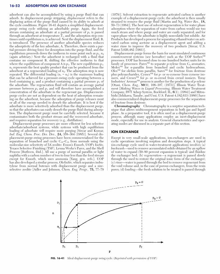
adsorbent can also be accomplished by using a purge fluid that canadsorb. In displacement-purge stripping, displacement refers to thedisplacing action of the purge fluid caused by its ability to adsorb atthe cycle conditions. Figure 16-41 depicts a simplified displacement-purge swing cycle utilizing an adsorbable purge. Again, the feedstream containing an adsorbate at a partial pressure of p1 is passedthrough an adsorbent at temperature T1, and the adsorption step con-tinues until equilibrium n1 is achieved. Next the displacement fluid, B,is introduced. The presence of another adsorbable species reducesthe adsorptivity of the key adsorbate, A. Therefore, there exists a par-tial pressure driving force for desorption into the purge fluid, and theequilibrium proceeds down the isotherm to some point such as p1, n2
(again arbitrary.) Next the adsorbent is recharged with a fluid thatcontains no component B, shifting the effective isotherm to thatwhere the equilibrium of component A is p3. The new equilibrium p3,n2 represents the best quality product that can be produced from theadsorbent at a regenerated loading of n2. The adsorption step is nowrepeated. The differential loading (n1 − n2) is the maximum loadingthat can be achieved for a pressure-swing cycle operating between afeed containing y1 and a product containing a partial pressure p3 of the adsorbate. The regeneration fluid will contain an average partialpressure between p2 and p1 and will therefore have accomplished aconcentration of the adsorbate in the regenerant gas. Displacement-purge cycles are not as dependent on the heat of adsorption remain-ing on the adsorbent, because the adsorption of purge releases mostor all of the energy needed to desorb the adsorbate. It is best if theadsorbate is more selectively adsorbed than the displacement purge,so that the adsorbates can easily desorb the purge fluid during adsorp-tion. The displacement purge must be carefully selected, because itcontaminates both the product stream and the recovered adsorbate,and requires separation for recovery (e.g., distillation).
Displacement-purge processes are more efficient for less selectiveadsorbate/adsorbent systems, while systems with high equilibriumloading of adsorbate will require more purging [Sircar and Kumar,Ind. Eng. Chem. Proc. Des. Dev., 24, 358–364 (1985)]. Several dis-placement-purge-swing processes have been commercialized for theseparation of branched and cyclic C10–C18 from normals using themolecular-size selectivity of 5A zeolite: Exxon’s Ensorb, UOP’s IsoSiv,Texaco Selective Finishing (TSF), Leuna Werke’s Parex, and the ShellProcess [Ruthven, ibid.]. All use a purge of normal paraffin or lightnaphtha with a carbon number of two to four less than the feed streamexcept for Ensorb, which uses ammonia [Yang, gen. refs.]. UOP has also developed a similar process, OlefinSiv, which separates isobu-tylene from normal butenes with displacement purge and a size-selective zeolite [Adler and Johnson, Chem. Eng. Progr., 75, 77–79
(1979)]. Solvent extraction to regenerate activated carbon is anotherexample of a displacement-purge cycle; the adsorbent is then usuallysteamed to remove the purge fluid [Martin and Ng, Water Res., 18,59–73 (1984)]. The best use of solvent regeneration is for water phaseadsorption where the separation of water from carbon would use toomuch steam and where purge and water are easily separated; and forvapor-phase where the adsorbate is highly nonvolatile but soluble. AirProducts has developed a process for separating ethanol/water on acti-vated carbon using acetone as a displacement agent and adding awater rinse to improve the recovery of two products [Sircar, U.S.Patent 5,026,482 (1991)].
Displacement-purge forms the basis for most simulated continuouscountercurrent systems (see hereafter) such as the UOP SorbexSM
processes. UOP has licensed close to one hundred Sorbex units for itsfamily of processes: ParexSM to separate p-xylene from C8 aromatics,MolexSM for n-paraffin from branched and cyclic hydrocarbons,OlexSM for olefins from paraffin, SarexSM for fructose from dextroseplus polysaccharides, CymexSM for p- or m-cymene from cymene iso-mers, and CresexSM for p- or m-cresol from cresol isomers. TorayIndustries’ AromaxSM process is another for the production of p-xylene[Otani, Chem. Eng., 80(9), 106–107, (1973)]. Illinois Water Treat-ment [Making Waves in Liquid Processing, Illinois Water TreatmentCompany, IWT Adsep System, Rockford, IL, 6(1), (1984)] and Mitsu-bishi [Ishikawa, Tanabe, and Usui, U.S. Patent 4,182,633 (1980)] havealso commercialized displacement-purge processes for the separationof fructose from dextrose.
Chromatography Chromatography is a sorptive separation tech-nique that allows multicomponent separations in both gas and liquidphase. As a preparative tool, it is often used as a displacement-purgeprocess, although many applications employ an inert-displacementmode, especially for use in analysis. General characteristics and oper-ating modes are discussed in a separate part of this section.
ION EXCHANGE
Except in very small-scale applications, ion-exchangers are used incyclic operations involving sorption and desorption steps. A typicalion-exchange cycle used in water-treatment applications involves (a)backwash—used to remove accumulated solids obtained by an upflowof water to expand (50–80 percent expansion is typical) and fluidizethe exchanger bed; (b) regeneration—a regenerant is passed slowlythrough the used to restore the original ionic form of the exchanger;(c) rinse—water is passed through the bed to remove regenerant fromthe void volume and, in the case of porous exchangers, from the resinpores; (d) loading—the fresh solution to be treated is passed through
16-52 ADSORPTION AND ION EXCHANGE
FIG. 16-41 Ideal displacement-purge swing cycle. (Reprinted with permission of UOP.)
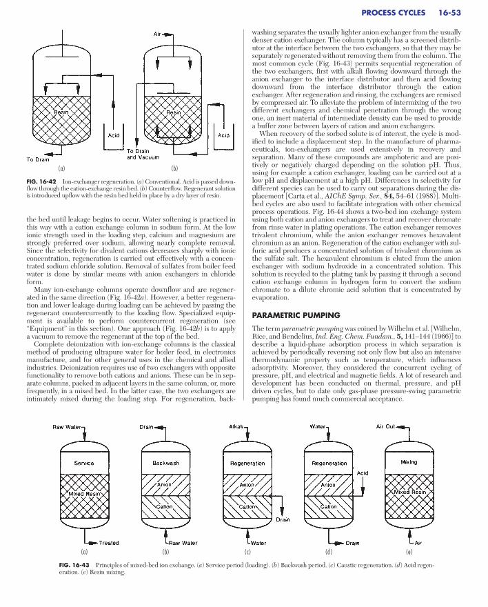
the bed until leakage begins to occur. Water softening is practiced inthis way with a cation exchange column in sodium form. At the lowionic strength used in the loading step, calcium and magnesium arestrongly preferred over sodium, allowing nearly complete removal.Since the selectivity for divalent cations decreases sharply with ionicconcentration, regeneration is carried out effectively with a concen-trated sodium chloride solution. Removal of sulfates from boiler feedwater is done by similar means with anion exchangers in chlorideform.
Many ion-exchange columns operate downflow and are regener-ated in the same direction (Fig. 16-42a). However, a better regenera-tion and lower leakage during loading can be achieved by passing theregenerant countercurrently to the loading flow. Specialized equip-ment is available to perform countercurrent regeneration (see“Equipment” in this section). One approach (Fig. 16-42b) is to applya vacuum to remove the regenerant at the top of the bed.
Complete deionization with ion-exchange columns is the classicalmethod of producing ultrapure water for boiler feed, in electronicsmanufacture, and for other general uses in the chemical and alliedindustries. Deionization requires use of two exchangers with oppositefunctionality to remove both cations and anions. These can be in sep-arate columns, packed in adjacent layers in the same column, or, morefrequently, in a mixed bed. In the latter case, the two exchangers areintimately mixed during the loading step. For regeneration, back-
washing separates the usually lighter anion exchanger from the usuallydenser cation exchanger. The column typically has a screened distrib-utor at the interface between the two exchangers, so that they may beseparately regenerated without removing them from the column. Themost common cycle (Fig. 16-43) permits sequential regeneration ofthe two exchangers, first with alkali flowing downward through theanion exchanger to the interface distributor and then acid flowingdownward from the interface distributor through the cationexchanger. After regeneration and rinsing, the exchangers are remixedby compressed air. To alleviate the problem of intermixing of the twodifferent exchangers and chemical penetration through the wrongone, an inert material of intermediate density can be used to providea buffer zone between layers of cation and anion exchangers.
When recovery of the sorbed solute is of interest, the cycle is mod-ified to include a displacement step. In the manufacture of pharma-ceuticals, ion-exchangers are used extensively in recovery andseparation. Many of these compounds are amphoteric and are posi-tively or negatively charged depending on the solution pH. Thus,using for example a cation exchanger, loading can be carried out at alow pH and displacement at a high pH. Differences in selectivity fordifferent species can be used to carry out separations during the dis-placement [Carta et al., AIChE Symp. Ser., 84, 54–61 (1988)]. Multi-bed cycles are also used to facilitate integration with other chemicalprocess operations. Fig. 16-44 shows a two-bed ion exchange systemusing both cation and anion exchangers to treat and recover chromatefrom rinse water in plating operations. The cation exchanger removestrivalent chromium, while the anion exchanger removes hexavalentchromium as an anion. Regeneration of the cation exchanger with sul-furic acid produces a concentrated solution of trivalent chromium asthe sulfate salt. The hexavalent chromium is eluted from the anionexchanger with sodium hydroxide in a concentrated solution. Thissolution is recycled to the plating tank by passing it through a secondcation exchange column in hydrogen form to convert the sodiumchromate to a dilute chromic acid solution that is concentrated byevaporation.
PARAMETRIC PUMPING
The term parametric pumping was coined by Wilhelm et al. [Wilhelm,Rice, and Bendelius, Ind. Eng. Chem. Fundam., 5, 141–144 (1966)] todescribe a liquid-phase adsorption process in which separation isachieved by periodically reversing not only flow but also an intensivethermodynamic property such as temperature, which influencesadsorptivity. Moreover, they considered the concurrent cycling ofpressure, pH, and electrical and magnetic fields. A lot of research anddevelopment has been conducted on thermal, pressure, and pHdriven cycles, but to date only gas-phase pressure-swing parametricpumping has found much commercial acceptance.
PROCESS CYCLES 16-53
FIG. 16-42 Ion-exchanger regeneration. (a) Conventional. Acid is passed down-flow through the cation-exchange resin bed. (b) Counterflow. Regenerant solutionis introduced upflow with the resin bed held in place by a dry layer of resin.
(b)(a)
FIG. 16-43 Principles of mixed-bed ion exchange. (a) Service period (loading). (b) Backwash period. (c) Caustic regeneration. (d) Acid regen-eration. (e) Resin mixing.
(a) (b) (c) (d ) (e)

16-54 ADSORPTION AND ION EXCHANGE
FIG. 16-44 Multicomponent ion-exchange process for chromate recovery from platingrinse water. (Adapted from Rhom & Haas with permission.)
FIG. 16-45 Flow diagram of desiccant cooling cycle. [Reprinted with permission of AmericanSociety of Heating, Refrigeration and Air Conditioning Engineers, Inc. (ASHRAE). Reference: Col-lier, Cohen, and Slosberg in Harrimam, Desiccant Cooling and Dehumidification, ASHRAE,Atlanta, 1992.]
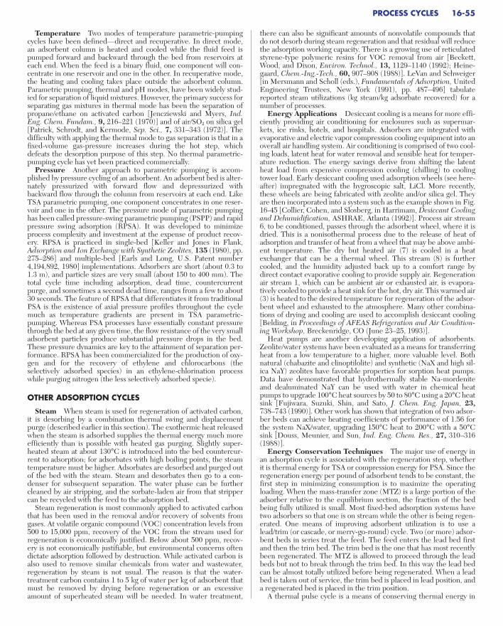
Temperature Two modes of temperature parametric-pumpingcycles have been defined—direct and recuperative. In direct mode,an adsorbent column is heated and cooled while the fluid feed ispumped forward and backward through the bed from reservoirs ateach end. When the feed is a binary fluid, one component will con-centrate in one reservoir and one in the other. In recuperative mode,the heating and cooling takes place outside the adsorbent column.Parametric pumping, thermal and pH modes, have been widely stud-ied for separation of liquid mixtures. However, the primary success forseparating gas mixtures in thermal mode has been the separation ofpropane/ethane on activated carbon [Jencziewski and Myers, Ind.Eng. Chem. Fundam., 9, 216–221 (1970)] and of air/SO2 on silica gel[Patrick, Schrodt, and Kermode, Sep. Sci., 7, 331–343 (1972)]. Thedifficulty with applying the thermal mode to gas separation is that in afixed-volume gas-pressure increases during the hot step, whichdefeats the desorption purpose of this step. No thermal parametric-pumping cycle has yet been practiced commercially.
Pressure Another approach to parametric pumping is accom-plished by pressure cycling of an adsorbent. An adsorbent bed is alter-nately pressurized with forward flow and depressurized withbackward flow through the column from reservoirs at each end. LikeTSA parametric pumping, one component concentrates in one reser-voir and one in the other. The pressure mode of parametric pumpinghas been called pressure-swing parametric pumping (PSPP) and rapidpressure swing adsorption (RPSA). It was developed to minimizeprocess complexity and investment at the expense of product recov-ery. RPSA is practiced in single-bed [Keller and Jones in Flank,Adsorption and Ion Exchange with Synthetic Zeolites, 135 (1980), pp.275–286] and multiple-bed [Earls and Long, U.S. Patent number4,194,892, 1980] implementations. Adsorbers are short (about 0.3 to1.3 m), and particle sizes are very small (about 150 to 400 mm). Thetotal cycle time including adsorption, dead time, countercurrentpurge, and sometimes a second dead time, ranges from a few to about30 seconds. The feature of RPSA that differentiates it from traditionalPSA is the existence of axial pressure profiles throughout the cyclemuch as temperature gradients are present in TSA parametric-pumping. Whereas PSA processes have essentially constant pressurethrough the bed at any given time, the flow resistance of the very smalladsorbent particles produce substantial pressure drops in the bed.These pressure dynamics are key to the attainment of separation per-formance. RPSA has been commercialized for the production of oxy-gen and for the recovery of ethylene and chlorocarbons (theselectively adsorbed species) in an ethylene-chlorination processwhile purging nitrogen (the less selectively adsorbed specie).
OTHER ADSORPTION CYCLES
Steam When steam is used for regeneration of activated carbon,it is desorbing by a combination thermal swing and displacementpurge (described earlier in this section). The exothermic heat releasedwhen the steam is adsorbed supplies the thermal energy much moreefficiently than is possible with heated gas purging. Slightly super-heated steam at about 130°C is introduced into the bed countercur-rent to adsorption; for adsorbates with high boiling points, the steamtemperature must be higher. Adsorbates are desorbed and purged outof the bed with the steam. Steam and desorbates then go to a con-denser for subsequent separation. The water phase can be furthercleaned by air stripping, and the sorbate-laden air from that strippercan be recycled with the feed to the adsorption bed.
Steam regeneration is most commonly applied to activated carbonthat has been used in the removal and/or recovery of solvents fromgases. At volatile organic compound (VOC) concentration levels from500 to 15,000 ppm, recovery of the VOC from the stream used forregeneration is economically justified. Below about 500 ppm, recov-ery is not economically justifiable, but environmental concerns oftendictate adsorption followed by destruction. While activated carbon isalso used to remove similar chemicals from water and wastewater,regeneration by steam is not usual. The reason is that the water-treatment carbon contains 1 to 5 kg of water per kg of adsorbent thatmust be removed by drying before regeneration or an excessiveamount of superheated steam will be needed. In water treatment,
there can also be significant amounts of nonvolatile compounds thatdo not desorb during steam regeneration and that residual will reducethe adsorption working capacity. There is a growing use of reticulatedstyrene-type polymeric resins for VOC removal from air [Beckett,Wood, and Dixon, Environ. Technol., 13, 1129–1140 (1992); Heine-gaard, Chem.-Ing.-Tech., 60, 907–908 (1988)]. LeVan and Schweiger[in Mersmann and Scholl (eds.), Fundamentals of Adsorption, UnitedEngineering Trustees, New York (1991), pp. 487–496] tabulatereported steam utilizations (kg steam/kg adsorbate recovered) for anumber of processes.
Energy Applications Desiccant cooling is a means for more effi-ciently providing air conditioning for enclosures such as supermar-kets, ice rinks, hotels, and hospitals. Adsorbers are integrated withevaporative and electric vapor compression cooling equipment into anoverall air handling system. Air conditioning is comprised of two cool-ing loads, latent heat for water removal and sensible heat for temper-ature reduction. The energy savings derive from shifting the latentheat load from expensive compression cooling (chilling) to coolingtower load. Early desiccant cooling used adsorption wheels (see here-after) impregnated with the hygroscopic salt, LiCl. More recently,these wheels are being fabricated with zeolite and/or silica gel. Theyare then incorporated into a system such as the example shown in Fig.16-45 [Collier, Cohen, and Slosberg, in Harrimam, Desiccant Coolingand Dehumidification, ASHRAE, Atlanta (1992)]. Process air stream6, to be conditioned, passes through the adsorbent wheel, where it isdried. This is a nonisothermal process due to the release of heat ofadsorption and transfer of heat from a wheel that may be above ambi-ent temperature. The dry but heated air (7) is cooled in a heatexchanger that can be a thermal wheel. This stream (8) is furthercooled, and the humidity adjusted back up to a comfort range bydirect contact evaporative cooling to provide supply air. Regenerationair stream 1, which can be ambient air or exhausted air, is evapora-tively cooled to provide a heat sink for the hot, dry air. This warmed air(3) is heated to the desired temperature for regeneration of the adsor-bent wheel and exhausted to the atmosphere. Many other combina-tions of drying and cooling are used to accomplish desiccant cooling[Belding, in Proceedings of AFEAS Refrigeration and Air Condition-ing Workshop, Breckenridge, CO (June 23–25, 1993)].
Heat pumps are another developing application of adsorbents. Zeolite/water systems have been evaluated as a means for transferringheat from a low temperature to a higher, more valuable level. Bothnatural (chabazite and clinoptilolite) and synthetic (NaX and high sil-ica NaY) zeolites have favorable properties for sorption heat pumps.Data have demonstrated that hydrothermally stable Na-mordeniteand dealuminated NaY can be used with water in chemical heatpumps to upgrade 100°C heat sources by 50 to 80°C using a 20°C heatsink [Fujiwara, Suzuki, Shin, and Sato, J. Chem. Eng. Japan, 23,738–743 (1990)]. Other work has shown that integration of two adsor-ber beds can achieve heating coefficients of performance of 1.56 forthe system NaX/water, upgrading 150°C heat to 200°C with a 50°Csink [Douss, Meunier, and Sun, Ind. Eng. Chem. Res., 27, 310–316(1988)].
Energy Conservation Techniques The major use of energy inan adsorption cycle is associated with the regeneration step, whetherit is thermal energy for TSA or compression energy for PSA. Since theregeneration energy per pound of adsorbent tends to be constant, thefirst step in minimizing consumption is to maximize the operatingloading. When the mass-transfer zone (MTZ) is a large portion of theadsorber relative to the equilibrium section, the fraction of the bedbeing fully utilized is small. Most fixed-bed adsorption systems havetwo adsorbers so that one is on stream while the other is being regen-erated. One means of improving adsorbent utilization is to use alead/trim (or cascade, or merry-go-round) cycle. Two (or more) adsor-bent beds in series treat the feed. The feed enters the lead bed firstand then the trim bed. The trim bed is the one that has most recentlybeen regenerated. The MTZ is allowed to proceed through the leadbeds but not to break through the trim bed. In this way the lead bedcan be almost totally utilized before being regenerated. When a leadbed is taken out of service, the trim bed is placed in lead position, anda regenerated bed is placed in the trim position.
A thermal pulse cycle is a means of conserving thermal energy in
PROCESS CYCLES 16-55

ADSORPTION
General Design Adsorbents are used in adsorbers with fixedinventory, with intermittent solids flow, or with continuous-movingsolids flow. The most common are fixed beds operating as batch unitsor as beds of adsorbent through which the feed fluid passes, with peri-odic interruption for regeneration. Total systems consist of pressurevessels or open tanks along with the associated piping, valves, controls,and auxiliary equipment needed to accomplish regeneration of theadsorbent. Gas treating equipment includes blowers or compressorswith a multiplicity of paths to prevent dead-heading. Liquid treatingequipment includes pumps with surge vessels as needed to assurecontinuous flow.
Adsorber Vessel The most frequently used method of fluid-solidcontact for adsorption operations is in cylindrical, vertical vessels, with
the adsorbent particles in a fixed and closely but randomly packedarrangement. The adsorbers must be designed with consideration forpressure drop and must contain a means of supporting the adsorbentand a means of assuring that the incoming fluid is evenly distributedto the face of the bed. There are additional design considerations foradsorbers when the streams are liquid and for high-performance sep-aration applications using very small particles (<0.05 mm) such as inHPLC.
For most large-scale processes, adsorbent particle size varies from0.06 to 6 mm (0.0025 to 0.25 in), but the adsorbent packed in a fixedbed will have a fairly narrow particle size range. Pressure drop inadsorbers can be changed by changing the diameter to bed depth ratioand by changing the particle size (see Sec. 5). Adsorbent size alsodetermines separation performance of adsorbent columns—increas-ing efficiency with decreasing particle size. In liquid-phase process-
heating-limited desorption. A process cycle that is heat-limited needsonly a very small time (dwell) at temperature to achieve satisfactorydesorption. If the entire bed is heated before the cooling is begun,every part of the bed will dwell at temperature for the entire time ittakes the cooling front to traverse the bed. Thus, much of the heat inthe bed at the start of cooling would be swept from the bed. Instead,cooling is begun before any heat front has exited the bed, creating athermal pulse that moves through the bed. The pulse expends its ther-mal energy for desorption so that only a small temperature peakremains at the end of the regeneration and no excess heat has beenwasted. If the heating step is stripping-limited, a thermal pulse is notapplicable.
A series cool/heat cycle is another way in which the heat that ispurged from the bed during cooling can be conserved. Sometimes theoutlet fluid is passed to a heat sink where energy is stored to be reusedto preheat heating fluid, or cross exchanged against the purge fluid torecover energy. However, there is also a process cycle that accom-plishes the same effect. Three adsorbers are used, with one on adsorp-tion, one on heating, and one on cooling. The regeneration fluid flowsin series, first to cool the bed just heated and then to heat the bed tobe desorbed. Thus all of the heat swept from the adsorber duringheating can be reused to reduce the heating requirement. Unlikethermal pulse, this cycle is applicable to both heat- and stripping-limited heating.
Process Selection The preceding sections present many processcycles and their variations. It is important to have some guidelines fordesign engineers to narrow their choice of cycles to the most econom-ical for a particular separation. Keller and coworkers [Keller et al.,gen. refs.] have presented a method for choosing appropriate adsorp-
tion processes. Their procedure considers the economics of capital,energy, labor, and other costs. Although these costs can vary from siteto site, the procedure is robust enough to include most scenarios. InTable 16-17, nine statements are made about the character of the sep-aration being considered. The numbers of the statements that are true(i.e., applicable) are used in the matrix in Table 16-18. A “no” for anytrue statement under a given process should remove that process fromfurther consideration. Any process having all “yes” answers for truestatements deserves strong consideration. Entries other than “yes” or“no” provide a means of prioritizing processes when more than onecycle is satisfactory.
16-56 ADSORPTION AND ION EXCHANGE
TABLE 16-17 Process Descriptors
Number Statement
1 Feed is a vaporized liquid or a gas.2 Feed is a liquid that can be fully vaporized at less than about
200°C.3 Feed is a liquid that cannot be fully vaporized at 200°C.4 Adsorbate concentration in the feed is less than about 3 wt %.5 Adsorbate concentration in the feed is between about 3 and 10 wt %.6 Adsorbate concentration in the feed is greater than about 10 wt %.7 Adsorbate must be recovered in high purity (> than 90–99%
rejection of nonadsorbed material).8 Adsorbate can be desorbed by thermal regeneration.9 Practical purge or displacement agents cannot be easily separated
from the adsorbate.
Keller, Anderson, and Yon in Rousseau (ed.), Handbook of Separation ProcessTechnology, John Wiley & Sons, Inc., New York, 1987; reprinted with permission.
TABLE 16-18 Process Selection Matrix
StatementGas- or vapor-phase processes Liquid-phase processes
number, Temperature Inert Displacement Pressure Chroma- Temperature Simulated Chroma-Table 16-17 swing purge purge swing tography swing* moving bed tography
1 Yes Yes Yes Yes Yes No No No2 Not likely Yes Yes Yes Yes Yes Yes Yes3 No No No No No Yes Yes Yes4 Yes Yes Not likely Not likely Not likely Yes Not likely Maybe5 Yes Yes Yes Yes Yes No Yes Yes6 No Yes Yes Yes Yes No Yes Yes7 Yes Yes Yes Maybe† Yes Yes Yes Yes8 Yes No No No No Yes‡ No No9 Maybe§ Not likely Not likely N/A Not likely Maybe§ Not likely Not likely
*Includes powdered, fixed-bed, and moving-bed processes.†Very high ratio of feed to desorption pressure (>10:1) will be required. Vacuum desorption will probably be necessary.‡If adsorbate concentration in the feed is very low, it may be practical to discard the loaded adsorbent or reprocess off-site.§If it is not necessary to recover the adsorbate, these processes are satisfactory.Keller, Anderson, and Yon in Rousseau (ed.), Handbook of Separation Process Technology, John Wiley & Sons, Inc., New York, 1987; reprinted with permission.
EQUIPMENT
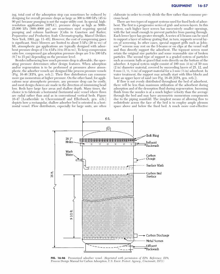
ing, total cost of the adsorption step can sometimes be reduced bydesigning for overall pressure drops as large as 300 to 600 kPa (45 to90 psi) because pumping is not the major utility cost. In special, high-resolution applications (HPLC), pressure drops as high as 5000–25,000 kPa (800–4000 psi) are sometimes used requiring specialpumping and column hardware [Colin in Ganetsos and Barker,Preparative and Production Scale Chromatography, Marcel Dekker,New York, 1993, pp. 11–45]. However, the cost of compressing gasesis significant. Since blowers are limited to about 5 kPa (20 in wc) oflift, atmospheric gas applications are typically designed with adsor-bent pressure drops of 1 to 4 kPa (4 to 16 in wc). To keep compressionratio low, compressed gas adsorption pressure drops are 5 to 100 kPa(0.7 to 15 psi) depending on the pressure level.
Besides influencing how much pressure drop is allowable, the oper-ating pressure determines other design features. When adsorptionand/or regeneration is to be performed at pressures above atmos-pheric, the adsorber vessels are designed like process pressure vessels(Fig. 16-46 [EPA, gen. refs.]). Their flow distributors can consumemore gas momentum at higher pressure. On the other hand, for appli-cations near atmospheric pressure, any pressure drop can be costly,and most design choices are made in the direction of minimizing headloss. Beds have large face areas and shallow depth. Many times, thechoice is to fabricate a horizontal (horizontal axis) vessel where flowsare radial rather than axial as in conventional vertical beds. Figure 16-47 [Leatherdale in Cheremisinoff and Ellerbusch, gen. refs.]depicts how a rectangular, shallow adsorber bed is oriented in a hori-zontal vessel. Flow distributors, especially for large units, are often
elaborate in order to evenly divide the flow rather than consume pre-cious head.
There are two types of support systems used for fixed beds of adsor-bent. The first is a progressive series of grid- and screen-layers. In thissystem, each higher layer screen has successively smaller openings,with the last small enough to prevent particles from passing through.Each lower layer has greater strength. A series of I-beams can be usedto support a layer of subway grating that, in turn, supports several lay-ers of screening. In other cases, special support grills such as John-sonTM screens may rest on the I-beams or on clips at the vessel walland thus directly support the adsorbent. The topmost screen mustretain the original size particles and some reasonable size of brokenparticles. The second type of support is a graded system of particlessuch as ceramic balls or gravel that rests directly on the bottom of theadsorber. A typical system might consist of 100 mm (4 in) of 50 mm (2 in) diameter material, covered by succeeding layers of 25, 12, and 6 mm (1, a, d in) of support material for a 3 mm (f in) adsorbent. Inwater treatment, the support may actually start with filter blocks andhave an upper layer of sand (see Fig. 16-48 [EPA, gen. refs.]).
If flow is not evenly distributed throughout the bed of adsorbent,there will be less than maximum utilization of the adsorbent duringadsorption and of the desorption fluid during regeneration. Incomingfluids from the nozzles is at a much higher velocity than the averagethrough the bed and may have asymmetric momentum componentsdue to the piping manifold. The simplest means of allowing flow toredistribute across the face of the bed is to employ ample plenumspace above and below the fixed bed. A much more cost-effective
EQUIPMENT 16-57
FIG. 16-46 Pressurized adsorber vessel. (Reprinted with permission of EPA. Reference: EPA,Process Design Manual for Carbon Adsorption, U.S. Envir. Protect. Agency., Cincinnati, 1973.)
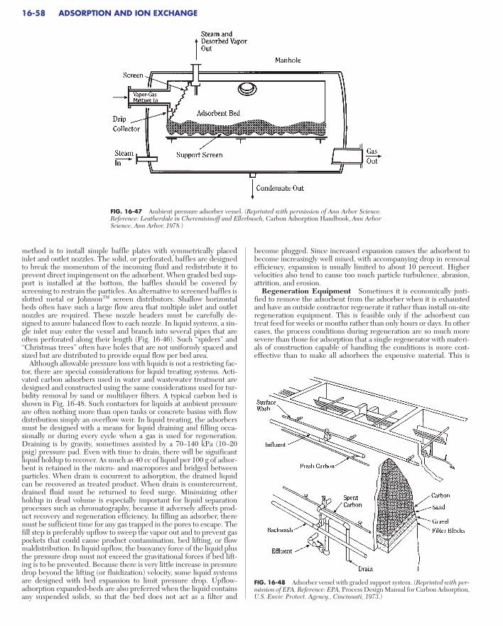
method is to install simple baffle plates with symmetrically placedinlet and outlet nozzles. The solid, or perforated, baffles are designedto break the momentum of the incoming fluid and redistribute it toprevent direct impingement on the adsorbent. When graded bed sup-port is installed at the bottom, the baffles should be covered byscreening to restrain the particles. An alternative to screened baffles isslotted metal or JohnsonTM screen distributors. Shallow horizontalbeds often have such a large flow area that multiple inlet and outletnozzles are required. These nozzle headers must be carefully de-signed to assure balanced flow to each nozzle. In liquid systems, a sin-gle inlet may enter the vessel and branch into several pipes that areoften perforated along their length (Fig. 16-46). Such “spiders” and“Christmas trees” often have holes that are not uniformly spaced andsized but are distributed to provide equal flow per bed area.
Although allowable pressure loss with liquids is not a restricting fac-tor, there are special considerations for liquid treating systems. Acti-vated carbon adsorbers used in water and wastewater treatment aredesigned and constructed using the same considerations used for tur-bidity removal by sand or multilayer filters. A typical carbon bed isshown in Fig. 16-48. Such contactors for liquids at ambient pressureare often nothing more than open tanks or concrete basins with flowdistribution simply an overflow weir. In liquid treating, the adsorbersmust be designed with a means for liquid draining and filling occa-sionally or during every cycle when a gas is used for regeneration.Draining is by gravity, sometimes assisted by a 70–140 kPa (10–20psig) pressure pad. Even with time to drain, there will be significantliquid holdup to recover. As much as 40 cc of liquid per 100 g of adsor-bent is retained in the micro- and macropores and bridged betweenparticles. When drain is cocurrent to adsorption, the drained liquidcan be recovered as treated product. When drain is countercurrent,drained fluid must be returned to feed surge. Minimizing otherholdup in dead volume is especially important for liquid separationprocesses such as chromatography, because it adversely affects prod-uct recovery and regeneration efficiency. In filling an adsorber, theremust be sufficient time for any gas trapped in the pores to escape. Thefill step is preferably upflow to sweep the vapor out and to prevent gaspockets that could cause product contamination, bed lifting, or flowmaldistribution. In liquid upflow, the buoyancy force of the liquid plusthe pressure drop must not exceed the gravitational forces if bed lift-ing is to be prevented. Because there is very little increase in pressuredrop beyond the lifting (or fluidization) velocity, some liquid systemsare designed with bed expansion to limit pressure drop. Upflow-adsorption expanded-beds are also preferred when the liquid containsany suspended solids, so that the bed does not act as a filter and
become plugged. Since increased expansion causes the adsorbent tobecome increasingly well mixed, with accompanying drop in removalefficiency, expansion is usually limited to about 10 percent. Highervelocities also tend to cause too much particle turbulence, abrasion,attrition, and erosion.
Regeneration Equipment Sometimes it is economically justi-fied to remove the adsorbent from the adsorber when it is exhaustedand have an outside contractor regenerate it rather than install on-siteregeneration equipment. This is feasible only if the adsorbent cantreat feed for weeks or months rather than only hours or days. In othercases, the process conditions during regeneration are so much moresevere than those for adsorption that a single regenerator with materi-als of construction capable of handling the conditions is more cost-effective than to make all adsorbers the expensive material. This is
16-58 ADSORPTION AND ION EXCHANGE
FIG. 16-47 Ambient pressure adsorber vessel. (Reprinted with permission of Ann Arbor Science.Reference: Leatherdale in Cheremisinoff and Ellerbusch, Carbon Adsorption Handbook, Ann ArborScience, Ann Arbor, 1978.)
FIG. 16-48 Adsorber vessel with graded support system. (Reprinted with per-mission of EPA. Reference: EPA, Process Design Manual for Carbon Adsorption,U.S. Envir. Protect. Agency., Cincinnati, 1973.)

true for most water and wastewater treatment with thermally reacti-vated carbon. Otherwise, desorption is conducted in situ with anyadditional equipment connected to the adsorbers.
Figure 16-49 [Engineering Data Book, 10th ed., Gas ProcessorsSuppliers Association, Tulsa, 1988, Sec. 20, p. 22] depicts the flowscheme for a typical two-bed TSA dryer system showing the auxiliaryequipment associated with regeneration. Some of the dry product gasis externally heated and used countercurrently to heat and desorbwater from the adsorber not currently drying feed. The wet, spentregeneration gas is cooled; the water is condensed out; and the gas isrecycled to feed for recovery.
The thermal reactivation of spent activated carbon may require thesame high temperatures and reaction conditions used for its manufac-ture. Although the exact conditions to be used for reactivation dependon the type of carbon and the adsorbates to be removed, the objectiveis to remove the adsorbed material without altering the carbon struc-ture. This occurs in four stages: (a) drying, (b) desorption, (c) pyroly-sis and carbonization, and (d) burnoff. Each of these steps isassociated with a particular temperature range and is carried out in amultiple hearth furnace such as that depicted in Fig. 16-50. This six-hearth system is a typical configuration for water treatment carbons.The gas temperature ranges from 100°C on the top hearth to 950°C atthe bottom. The rotating rabble arms rake the carbon from hearth tohearth. Wet, spent carbon is fed to the top, where it is dried by the toptwo hearths. Pyrolysis (desorption and decomposition) is accom-plished on the next hearth. The bottom four hearths are for reactiva-tion. Varying amounts of air, steam, and/or fuel are added to thedifferent hearths to maintain the conditions established for the partic-ular reactivation. A hearth area requirement of 0.1 m2/kg/hr (0.5 ft2/lb/hr) is adequate for cost estimating, but there are also detaileddesign procedures available [von Dreusche in Cheremisinoff andEllerbusch, gen. refs.].
In addition to the multiple-hearth furnace, the reactivation systemis comprised of additional equipment to transport, store, dewater, andquench the carbon.
A typical two-bed PSA dryer process flow scheme is very similar toFig. 16-49 without the regeneration gas heater. A portion of the dryproduct gas is used countercurrently to purge the water from theadsorber not currently drying feed. Again, the wet, spent purge gas iscooled, and the water is condensed out and recycled to feed for recov-ery. If the cycle is VSA, then instead of the regeneration gas compres-sor, there is a vacuum compressor at the purge outlet upstream of theregeneration cooler. Some PSA cycles such as in air-brake dryersoperate with one adsorber, a surge volume, and a three-way valve to
switch between pressurizing and countercurrent blowdown. Theother extreme of complexity is demonstrated by the UOP nine-bedPolybed PSA H2 unit shown in Fig. 16-51 [Fuderer and Rudelstorfer,U.S. Patent number 3,986,849, 1976]. This cycle requires nine adsor-bers sequenced by fifty-five valves to maximize purity and recovery.
Cycle Control Valves are the heart of cycle control for cyclicadsorption systems. These on/off valves switch flows among beds so
EQUIPMENT 16-59
FIG. 16-49 Two-bed TSA system with regeneration equipment. (Reprinted with permission ofGPSA. Reference: Engineering Data Book, 10th ed., Gas Processors Suppliers Association, Tulsa,1988, Sec. 20, p. 22.)
FIG. 16-50 Multiple hearth furnace for carbon reactivation. (Reprinted withpermission of EPA. Reference: EPA, Process Design Manual for Carbon Adsorp-tion, U.S. Envir. Protect. Agency., Cincinnati, 1973.)

that external to the system it appears as if operation is continuous. Ingeneral, one valve is needed for each bed at each end for each stepthat is performed (e.g., for a two-bed system with an adsorption stepplus heating and cooling step [carried out in the same direction andduring the same step], only 2 × 2 × 2 = 8 valves would be needed [seeFig. 16-49]). In some cycles such as pressure-swing systems, it may bepossible to use valves for more than one function (e.g., repressuriza-tion with feed gas using the same manifold as adsorption feed). With-out multiple use, the cycle in Fig. 16-51 would need 9 × 2 × 5 = 90valves instead of 55 to accommodate the five steps of adsorption,purge to product, blowdown, purge, and feed repressurization (evenwithout the equalization). For some applications, 3- and 4-way valvescan replace two and four valves, respectively. The ultimate integrationof switching valves is the UOP rotary valve discussed below. For longstep times (8 hours or more) it is possible for the valves to be manually
switched by operators. For most systems, it is advantageous for theopening and closing of the valves be controlled by automatic timers.The same controller can be responsible for maintaining flows andpressure, logic for proceeding only on completion of events, andsafety bypass or shutdown. Automatic control can provide for a periodof parallel flow paths to assure transitions. In some applications,process analyzers can interface with the controller to initiate bed-switching when adsorbate is detected breaking through into the effluent.
Continuous Countercurrent Systems Most adsorption sys-tems use fixed-bed adsorbers. However, if the fluid to be separatedand that used for desorption can be countercurrently contacted by amoving bed of the adsorbent, there are significant efficiencies to berealized. Because the adsorbent leaves the adsorption section essen-tially in equilibrium with the feed composition, the inefficiency of the
16-60 ADSORPTION AND ION EXCHANGE
FIG. 16-51 UOP nine-bed polybed PSA H2 unit: (a) flow scheme; (b) cycle diagram. (Reference: Fuderer and Rudelstorfer, U.S. Patentnumber 3,986,849, 1976.)

mass-transfer zone is eliminated. The adsorption section only needs tocontain a MTZ length of adsorbent compared to a MTZ plus an equi-librium section in a fixed bed. Likewise, countercurrent regenerationis more efficient. Since the adsorbent is moved from an adsorptionchamber to another chamber for regeneration, only the regenerationsection is designed for the often more severe conditions. Countercur-rent adsorption can take advantage of an exceptionally favorable equi-librium in water softening; and the regeneration step can be madefavorable by the use of relatively concentrated elutent. Continuousunits generally require more headroom but much less footprint. Theforemost problems to be overcome in the design and operation of con-tinuous countercurrent sorption operations are the mechanical com-plexity of equipment and the attrition of the sorbent.
An early example of a commercial countercurrent adsorptionprocesses is the hypersorption process developed by Union Oil Com-pany for the recovery of propane and heavier components from natural gas [Berg, Chem. Eng. Progr., 47, 585–590 (1951)]. Hyper-sorption used an activated carbon adsorbent moving as a dense bedcontinuously downward through a rising gas stream (Fig. 16-52 [Berg,ibid.]). However, this process proved to be less economical than cryo-genic distillation and had excessive carbon losses resulting from attri-tion. The commercialization by Kureha Chemical Co. of Japan of anew, highly attrition-resistant, activated-carbon adsorbent, alloweddevelopment of a process employing fluidized-bed adsorption andmoving bed desorption for removal of VOC compounds from air. Theprocess has been marketed as GASTAKSM in Japan and as PuraSivSM
HR (Fig. 16-53 [Anon., Chem. Eng., 84(18), 39–40 (1977)]) in theUnited States, and now as SOLDACS by Daikin Industries, Ltd. A
similar process using beaded polymeric resin is offered by Chematur[Heinegaard, Chem.-Ing.-Tech., 60, 907–908 (1988)]. The recent dis-covery [Acharya and BeVier, U.S. Patent number 4,526,877, 1985]that the graphite coating of zeolites can dramatically improve attritionresistance without significantly impairing adsorption performancecould allow the extension of moving-bed technology to other separa-tions. A good review of continuous ion-exchange applications is pre-sented by Wankat [gen. refs.].
Continuous Cross-Flow Systems There are at least threeimplementations of moving-bed adsorption that are cross flow ratherthan fixed beds or countercurrent flow: (1) panel beds, (2) adsorbentwheels, and (3) rotating annular beds. By cross flow is meant that theadsorbent is moving in a direction perpendicular to the fluid flow. Allof these employ moving adsorbent—the first, a down-flowing solid;and the others, a constrained solid. Panel beds of activated carbon likethose depicted in Fig. 16-54 [Lovett and Cunniff, Chem. Eng. Progr.,70(5), 43–47 (1974)] have been applied to odor control [Lovett andCunniff, ibid.] and to the desulfurization of waste gas [Richter,Knoblauch, and Juntgen, Verfahrenstechnik (Mainz), 14, 338–342(1980)]. The spent solid falls from the bottom panel into a load-outbin, and fresh regenerated carbon is added to the top; gas flowsthrough as shown.
The heart of an adsorbent wheel system is a rotating cylinder con-taining the adsorbent. Figure 16-55 illustrates two types: horizontaland vertical. In some adsorbent wheels, the adsorbent particles areplaced in basket segments (a multitude of fixed beds) to form a hori-
EQUIPMENT 16-61
FIG. 16-52 Hypersorption adsorber vessel [Reprinted with permission ofAIChE. Reference: Berg, Chem. Eng. Progr., 47, 585–590 (1951).]
FIG. 16-53 PuraSiv HR adsorber vessel. [Reprinted with permission of Chem-ical Engineering. Reference: Anon., Chem. Eng., 84(18), 39–40 (1977).]

zontal wheel that rotates around a vertical axis. In other instances, theadsorbent is integral to the monolithic wheel or coated onto a metal,paper, or ceramic honeycomb substrate. These monolithic or honey-comb structures rotate around either a vertical or a horizontal axis.The gas to be treated usually flows through the wheel parallel to theaxis of rotation, although some implementations use radial flow con-
figurations. Most of the wheel is removing adsorbates. The remaining(smaller) portion of the wheel is undergoing thermal regeneration—usually countercurrently. The wheel constantly rotates to provide acontinuous treated stream and a steady concentrated stream. Adsor-bent wheels are most often used to treat ambient air because theyhave very low pressure drop. One application of wheels is the removalof VOC where the regeneration stream is usually sent to an incinera-tor for destruction of VOC. Another use is in desiccant cooling (seepreviously). They do suffer from low efficiency due to the short con-tact time, mechanical leakage at seals, and the tendency to allow thewheel to exceed breakthrough in order to get better adsorbent utiliza-tion. Some adsorbent wheels are operated in an intermittent mannersuch that the wheel periodically indexes to a new position; this is par-ticularly true of radial flow wheels.
The rotating annular bed system for liquid chromatographic sepa-ration (two-dimensional chromatography) is analogous to the horizon-tal adsorbent wheel for gases. Feed to be separated flows to a portionof the top face of an annular bed of sorbent. A displacement purge inthe form of a solvent or carrier gas flows to the rest of the annulus. Theless strongly adsorbed components travel downward through the sor-bent at a higher rate. Thus, they will exit at the bottom of the annulusat a smaller angular distance from the feed sector. The more stronglyadsorbed species will exit at a greater angle. The mechanical andpacking complexities of such an apparatus have been overcome for apressurized system by workers at the Oak Ridge National Laboratoryshown in Fig. 16-56 [Canon, Begovich, and Sisson, Sep. Sci. Technol.,15, 655–678 (1980)]. Several potential applications are reviewed byCarta and Byers [Chromatographic and Membrane Processes inBiotechnology, NATO ASI Proceeding, Kluwer, 1991].
Simulated Continuous Countercurrent Systems Because ofthe problems associated with moving adsorbent in true continuouscountercurrent mode, most commercial application of continuouscountercurrent processes has been accomplished by using flowschemes that simulates the flow of adsorbent and process fluid. Thereare at least four types of implementation: (1) units designed to inter-mittently move the adsorbent rather than continuously, (2) continu-ously operating chromatographic columns to which the feed isperiodically pulsed, (3) enhancement of the chromatographic separa-tion by dividing the column and using recycles, and (4) moving thepoint of introduction of the feed and regeneration point along a seriesof beds.
Pulsed beds of activated carbon are used in water and wastewatertreatment systems. The adsorber tank is usually a vertical cylindricalpressure vessel, with fluid distributors at top and bottom, similar tothe arrangement of an ion exchanger. The column is filled with gran-ular carbon. Fluid flow is upward, and carbon is intermittently dis-
16-62 ADSORPTION AND ION EXCHANGE
FIG. 16-54 Cross-flow panel-bed adsorber. [Reprinted with permission ofAIChE. Reference: Lovett and Cunniff, Chem. Eng. Progr., 70(5), 43–47 (1974).]
FIG. 16-55 Adsorbent wheels for gas separation: (a) horizontal with fixed beds; (b) vertical monolith. (Reprinted with permissionof UOP.)
(b)(a)

placed downward by opening a valve at the bottom and injecting ameasured slug of carbon into the top of the vessel. The exhausted slug(a small fraction of the total charge in order to approximate fully coun-tercurrent operation very closely) is transferred to the sweeten-offtank, where residual product is displaced. It next is dewatered and fedto the regeneration furnace. The carbon is eventually returned to theadsorber where fluid flow is interrupted briefly to permit carbontransfer in, as in continuous ion exchanger systems.
Liquid chromatography has been used commercially to separateglucose from fructose and other sugar isomers, for recovery of nucleicacids, and other uses. A patent to Sanmatsu Kogyo Co., Ltd [Yoritomi,Kezuka, and Moriya, U.S. Patent number 4,267,054, 1981] presentsan improved chromatographic process that is simpler to build andoperate than simulated moving-bed processes. Figure 16-57 [Keller etal., gen. refs.] diagrams its use for a binary separation. It is a displace-ment-purge cycle where pure component cuts are recovered, whilecuts that contain both components are recycled to the feed end of thecolumn.
The UOP CyclesorbSM is another adsorptive separation processwith semicontinuous recycle. It utilizes a series of chromatographiccolumns to separate fructose from glucose. A series of internal recyclestreams of impure and dilute portions of the chromatograph are usedto improve the efficiency [Gerhold, U.S. Patent numbers 4,402,832,1983; and 4,478,721, 1984]. A schematic diagram of a six-vessel UOPCyclesorb process is shown in Fig. 16-58 [Gembicki et al., gen. refs.,p. 595]. The process has four external streams and four internal recy-cles: Dilute raffinate and impure extract are like displacement steps;and impure raffinate and dilute extract are recycled from the bottomof an adsorber to its top. Feed and desorbent are fed to the top of eachcolumn in a predetermined sequence. The switching of the feed anddesorbent are accomplished by the same rotary valve used for Sorbexswitching (see hereafter). A chromatographic profile is established ineach column that is moving from top to bottom, and all portions of anadsorber are performing a useful function at any time.
The concept of a simulated moving bed (SMB) was originally usedin a process developed and licensed under the name UOP Sorbexprocess [Broughton, Bieser, and Anderson, Pet. Int. (Milan), 23(3), p. 91 (1976); Broughton, Bieser, and Persak, Pet. Int. (Milan), 23(5),p. 36 (1976)]. The following discussion is based on that process, butthe concepts can be generally applied. In a moving-bed system forcontinuous countercurrent effect, solids move continuously in aclosed loop past fixed points of introduction and withdrawal of feedand regenerant. The same effect can be achieved by holding the bedstationary and periodically moving the points of introduction andwithdrawal of the various streams. Shifting those points in the direc-tion of fluid flow simulates the movement of solid in the oppositedirection. Since moving the positions continuously is impractical, afinite number of access lines are provided to a limited series of adsor-bent beds. The Sorbex commercial application of this concept is por-trayed in Fig. 16-59, which shows the adsorbent as a stationary bedand the auxiliary distillation columns needed to separate the desor-bent from raffinate and extract so that it can be recycled to theprocess. In this example, feed flows through the three beds of Zone 1,where the most strongly adsorbed component A is adsorbed anddepleted from the raffinate. Desorbent flows through the three bedsof Zone 3 to displace component A into the extract. The less stronglyadsorbed component B is adsorbed slightly in the two beds of Zone 4between raffinate outlet and desorbent, inlet to prevent it from con-taminating extract in Zone 3. Component B is desorbed in the fourbeds of Zone 2 between the extract outlet and the feed inlet and mostleaves with the raffinate. A pump draws liquid from the bottom outletto the top inlet of the adsorbent chamber. All flows in the beds aredownward, simulating an upward flow of solid. The four active portpositions are likewise moved downward by the selection of the rotaryvalve. The rotary valve functions in the same manner as a multiportstopcock or chromatography valve, sequencing the four streams onthe right to the lines connected to the inlet/outlet nozzles on theadsorber. The next position of the rotary valve will direct desorbent to
EQUIPMENT 16-63
FIG. 16-56 Annular bed for liquid separation. [Reprinted with permission of Marcel Dekker. Reference:Canon, Begovich, and Sisson, Sep. Sci. Technol., 15, 655–678 (1980).]
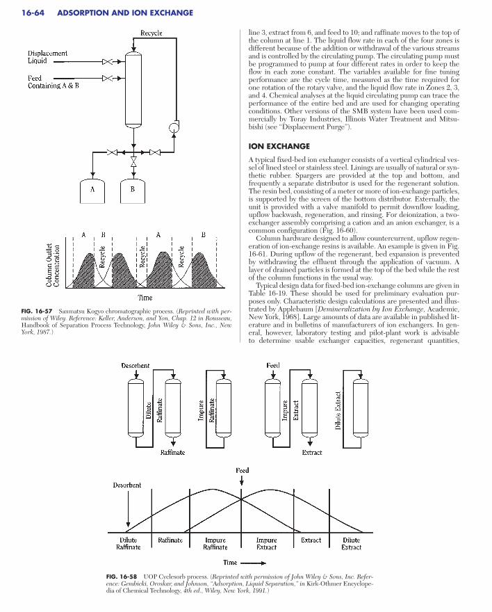
line 3, extract from 6, and feed to 10; and raffinate moves to the top ofthe column at line 1. The liquid flow rate in each of the four zones isdifferent because of the addition or withdrawal of the various streamsand is controlled by the circulating pump. The circulating pump mustbe programmed to pump at four different rates in order to keep theflow in each zone constant. The variables available for fine tuning performance are the cycle time, measured as the time required forone rotation of the rotary valve, and the liquid flow rate in Zones 2, 3,and 4. Chemical analyses at the liquid circulating pump can trace theperformance of the entire bed and are used for changing operatingconditions. Other versions of the SMB system have been used com-mercially by Toray Industries, Illinois Water Treatment and Mitsu-bishi (see “Displacement Purge”).
ION EXCHANGE
A typical fixed-bed ion exchanger consists of a vertical cylindrical ves-sel of lined steel or stainless steel. Linings are usually of natural or syn-thetic rubber. Spargers are provided at the top and bottom, andfrequently a separate distributor is used for the regenerant solution.The resin bed, consisting of a meter or more of ion-exchange particles,is supported by the screen of the bottom distributor. Externally, theunit is provided with a valve manifold to permit downflow loading,upflow backwash, regeneration, and rinsing. For deionization, a two-exchanger assembly comprising a cation and an anion exchanger, is acommon configuration (Fig. 16-60).
Column hardware designed to allow countercurrent, upflow regen-eration of ion-exchange resins is available. An example is given in Fig.16-61. During upflow of the regenerant, bed expansion is preventedby withdrawing the effluent through the application of vacuum. Alayer of drained particles is formed at the top of the bed while the restof the column functions in the usual way.
Typical design data for fixed-bed ion-exchange columns are given inTable 16-19. These should be used for preliminary evaluation pur-poses only. Characteristic design calculations are presented and illus-trated by Applebaum [Demineralization by Ion Exchange, Academic,New York, 1968]. Large amounts of data are available in published lit-erature and in bulletins of manufacturers of ion exchangers. In gen-eral, however, laboratory testing and pilot-plant work is advisable to determine usable exchanger capacities, regenerant quantities,
16-64 ADSORPTION AND ION EXCHANGE
FIG. 16-57 Sanmatsu Kogyo chromatographic process. (Reprinted with per-mission of Wiley. Reference: Keller, Anderson, and Yon, Chap. 12 in Rousseau,Handbook of Separation Process Technology, John Wiley & Sons, Inc., NewYork, 1987.)
FIG. 16-58 UOP Cyclesorb process. (Reprinted with permission of John Wiley & Sons, Inc. Refer-ence: Gembicki, Oroskar, and Johnson, “Adsorption, Liquid Separation,” in Kirk-Othmer Encyclope-dia of Chemical Technology, 4th ed., Wiley, New York, 1991.)
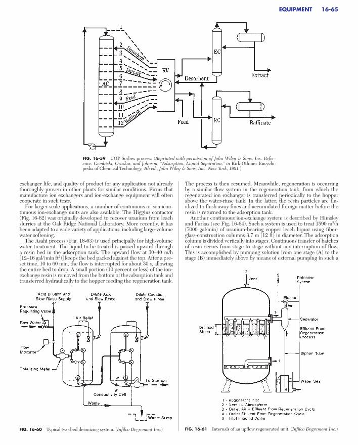
exchanger life, and quality of product for any application not alreadythoroughly proven in other plants for similar conditions. Firms thatmanufacture ion exchangers and ion-exchange equipment will oftencooperate in such tests.
For larger-scale applications, a number of continuous or semicon-tinuous ion-exchange units are also available. The Higgins contactor(Fig. 16-62) was originally developed to recover uranium from leachslurries at the Oak Ridge National Laboratory. More recently, it hasbeen adapted to a wide variety of applications, including large-volumewater softening.
The Asahi process (Fig. 16-63) is used principally for high-volumewater treatment. The liquid to be treated is passed upward through a resin bed in the adsorption tank. The upward flow at 30–40 m/h[12–16 gal/(min ft2)] keeps the bed packed against the top. After a pre-set time, 10 to 60 min, the flow is interrupted for about 30 s, allowingthe entire bed to drop. A small portion (10 percent or less) of the ion-exchange resin is removed from the bottom of the adsorption tank andtransferred hydraulically to the hopper feeding the regeneration tank.
The process is then resumed. Meanwhile, regeneration is occurringby a similar flow system in the regeneration tank, from which theregenerated ion exchanger is transferred periodically to the hopperabove the water-rinse tank. In the latter, the resin particles are flu-idized to flush away fines and accumulated foreign matter before theresin is returned to the adsorption tank.
Another continuous ion-exchange system is described by Himsleyand Farkas (see Fig. 16-64). Such a system is used to treat 1590 m3/h(7000 gal/min) of uranium-bearing copper leach liquor using fiber-glass-construction columns 3.7 m (12 ft) in diameter. The adsorptioncolumn is divided vertically into stages. Continuous transfer of batchesof resin occurs from stage to stage without any interruption of flow.This is accomplished by pumping solution from one stage (A) to thestage (B) immediately above by means of external pumping in such a
EQUIPMENT 16-65
FIG. 16-59 UOP Sorbex process. (Reprinted with permission of John Wiley & Sons, Inc. Refer-ence: Gembicki, Oroskar, and Johnson, “Adsorption, Liquid Separation,” in Kirk-Othmer Encyclo-pedia of Chemical Technology, 4th ed., John Wiley & Sons, Inc., New York, 1991.)
FIG. 16-60 Typical two-bed deionizing system. (Infilco Degremont Inc.) FIG. 16-61 Internals of an upflow regenerated unit. (Infilco Degremont Inc.)
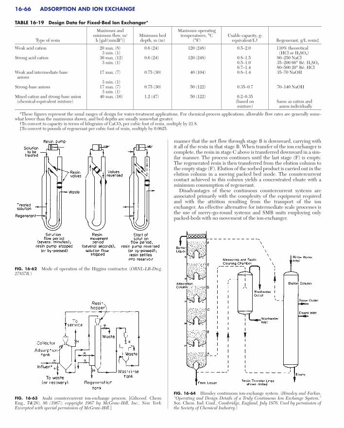
16-66 ADSORPTION AND ION EXCHANGE
TABLE 16-19 Design Data for Fixed-Bed Ion Exchanger*
Maximum and Maximum operatingminimum flow, m/ Minimum bed temperatures, °C Usable capacity, g-
Type of resin h [gal/(min⋅ft2)] depth, m (in) (°F) equivalent/L† Regenerant, g/L resin‡
Weak acid cation 20 max. (8) 0.6 (24) 120 (248) 0.5–2.0 110% theoretical3 min. (1) (HCl or H2SO4)
Strong acid cation 30 max. (12) 0.6 (24) 120 (248) 0.8–1.5 80–250 NaCl3 min. (1) 0.5–1.0 35–200 66° Bé. H2SO4
0.7–1.4 80–500 20° Bé. HClWeak and intermediate base 17 max. (7) 0.75 (30) 40 (104) 0.8–1.4 35–70 NaOHanions
3 min. (1)Strong-base anions 17 max. (7) 0.75 (30) 50 (122) 0.35–0.7 70–140 NaOH
3 min. (1)Mixed cation and strong-base anion 40 max. (16) 1.2 (47) 50 (122) 0.2–0.35(chemical-equivalent mixture) (based on Same as cation and
mixture) anion individually
*These figures represent the usual ranges of design for water-treatment applications. For chemical-process applications, allowable flow rates are generally some-what lower than the maximums shown, and bed depths are usually somewhat greater.
†To convert to capacity in terms of kilograins of CaCO3 per cubic foot of resin, multiply by 21.8.‡To convert to pounds of regenerant per cubic foot of resin, multiply by 0.0625.
FIG. 16-63 Asahi countercurrent ion-exchange process. [Gilwood, Chem.Eng., 74(26), 86 (1967); copyright 1967 by McGraw-Hill, Inc., New York.Excerpted with special permission of McGraw-Hill.]
FIG. 16-64 Himsley continuous ion-exchange system. (Himsley and Farkas,“Operating and Design Details of a Truly Continuous Ion Exchange System,”Soc. Chem. Ind. Conf., Cambridge, England, July 1976. Used by permission ofthe Society of Chemical Industry.)
FIG. 16-62 Mode of operation of the Higgins contractor. (ORNL-LR-Dwg.27857R.)
manner that the net flow through stage B is downward, carrying withit all of the resin in that stage B. When transfer of the ion exchanger iscomplete, the resin in stage C above is transferred downward in a sim-ilar manner. The process continues until the last stage (F) is empty.The regenerated resin is then transferred from the elution column tothe empty stage (F). Elution of the sorbed product is carried out in theelution column in a moving packed bed mode. The countercurrentcontact achieved in this column yields a concentrated eluate with aminimum consumption of regenerant.
Disadvantages of these continuous countercurrent systems areassociated primarily with the complexity of the equipment requiredand with the attrition resulting from the transport of the ionexchanger. An effective alternative for intermediate scale processes isthe use of merry-go-round systems and SMB units employing onlypacked-beds with no movement of the ion-exchanger.