admissible statistics from a latent variable perspective · admissible statistics from a latent...
TRANSCRIPT

UvA-DARE is a service provided by the library of the University of Amsterdam (http://dare.uva.nl)
UvA-DARE (Digital Academic Repository)
Admissible statistics from a latent variable perspective
Zand Scholten, A.
Link to publication
Citation for published version (APA):Zand Scholten, A. (2011). Admissible statistics from a latent variable perspective
General rightsIt is not permitted to download or to forward/distribute the text or part of it without the consent of the author(s) and/or copyright holder(s),other than for strictly personal, individual use, unless the work is under an open content license (like Creative Commons).
Disclaimer/Complaints regulationsIf you believe that digital publication of certain material infringes any of your rights or (privacy) interests, please let the Library know, statingyour reasons. In case of a legitimate complaint, the Library will make the material inaccessible and/or remove it from the website. Please Askthe Library: http://uba.uva.nl/en/contact, or a letter to: Library of the University of Amsterdam, Secretariat, Singel 425, 1012 WP Amsterdam,The Netherlands. You will be contacted as soon as possible.
Download date: 01 Jul 2018


ADMISSIBLE STATISTICS FROM A
LATENT VARIABLE PERSPECTIVE
ANNEMARIE ZAND SCHOLTEN

ADMISSIBLE STATISTICS
FROM A LATENT VARIABLE PERSPECTIVE
ACADEMISCH PROEFSCHRIFT
ter verkrijging van de graad van doctor
aan de Universiteit van Amsterdam
op gezag van de Rector Magnificus
prof. dr. D.C. van den Boom
ten overstaan van een door het college voor promoties ingestelde
commissie, in het openbaar te verdedigen in de Agnietenkapel
op vrijdag 21 januari 2011, te 12:00 uur
door
Annemarie Zand Scholten
geboren te Haarlem

PROMOTIECOMMISSIE:
Promotor: Prof. dr. H.L.J. van der Maas
Copromotores: Dr. D. Borsboom
Dr. P. Koele
Overige leden: Prof. dr. P.A.L. de Boeck
Prof. dr. G.K.J. Maris
Prof. dr. K. Sijtsma
Prof. dr. H. Kelderman
Dr. E.M. Wagenmakers
Faculteit der Maatschappij- en Gedragswetenschappen

voor Zand Scholten en Prins

Contents
Acknowledgements xi
Preface xv
1 Introduction 1
1.1 Measurement in Psychology . . . . . . . . . . . . . . . . . . . . 1
1.2 Admissible Statistics . . . . . . . . . . . . . . . . . . . . . . . . 3
1.3 Representational Measurement Theory . . . . . . . . . . . . . 4
1.4 Latent Variable Models . . . . . . . . . . . . . . . . . . . . . . . 5
1.5 Overview . . . . . . . . . . . . . . . . . . . . . . . . . . . . . . . 7
2 A Reanalysis of Lord’s Statistical Treatment of Football Numbers 11
2.1 Admissible Statistics . . . . . . . . . . . . . . . . . . . . . . . . 12
2.2 The Treatment of Football Numbers . . . . . . . . . . . . . . . 15
2.3 Vending Machine Bias . . . . . . . . . . . . . . . . . . . . . . . 19
vii
2.4 Conclusion . . . . . . . . . . . . . . . . . . . . . . . . . . . . . . 24
3 The Rasch Model as Additive Conjoint Measurement 29
3.1 Measurement Levels and Admissible Statistics . . . . . . . . . 30
3.2 Representational Measurement Theory . . . . . . . . . . . . . 32
3.3 Assumptions of Latent Variable Models . . . . . . . . . . . . . 36
3.4 Rasch and Additive Conjoint Measurement . . . . . . . . . . . 38
3.5 Conclusion . . . . . . . . . . . . . . . . . . . . . . . . . . . . . . 45
4 The Guttman-Rasch Paradox in Item Response Theory 47
4.1 Measurement Level Difference in IRT Models . . . . . . . . . . 48
4.2 Guttman and Rasch . . . . . . . . . . . . . . . . . . . . . . . . . 50
4.3 Measurement Pretensions . . . . . . . . . . . . . . . . . . . . . 53
4.4 Why Guttman Fails to Yield Interval Measurement . . . . . . . 55
4.5 Rasch Is Guttman Plus Error . . . . . . . . . . . . . . . . . . . . 59
4.6 Error that Improves Precision . . . . . . . . . . . . . . . . . . . 61
4.7 Error and Precision in the Rasch Model . . . . . . . . . . . . . 66
4.8 Discussion . . . . . . . . . . . . . . . . . . . . . . . . . . . . . . 69
5 How to Avoid Misinterpretation of Interaction Effects 73
5.1 Arbitrary Interactions . . . . . . . . . . . . . . . . . . . . . . . . 74
5.2 Method . . . . . . . . . . . . . . . . . . . . . . . . . . . . . . . . 86
5.3 Results . . . . . . . . . . . . . . . . . . . . . . . . . . . . . . . . 89
5.4 Assessing Risk . . . . . . . . . . . . . . . . . . . . . . . . . . . . 96
5.5 Discussion . . . . . . . . . . . . . . . . . . . . . . . . . . . . . . 99
viii

Contents ix
6 The Interpretation of Interactions Based on Polytomous Items 101
6.1 Introduction . . . . . . . . . . . . . . . . . . . . . . . . . . . . . 102
6.2 Simulation Study . . . . . . . . . . . . . . . . . . . . . . . . . . 105
6.3 Method . . . . . . . . . . . . . . . . . . . . . . . . . . . . . . . . 106
6.4 Results . . . . . . . . . . . . . . . . . . . . . . . . . . . . . . . . 110
6.5 Discussion . . . . . . . . . . . . . . . . . . . . . . . . . . . . . . 119
7 Discussion 121
7.1 Summary . . . . . . . . . . . . . . . . . . . . . . . . . . . . . . . 121
7.2 Conclusion . . . . . . . . . . . . . . . . . . . . . . . . . . . . . . 130
A A Bisymmetrical Structure for Vending Machine Bias 135
B The Axioms of ACM Applied to the Guttman and Rasch Models 139
C Types of Interactions According to Group Mean Ordering 145
References 151
Dutch Summary/Samenvatting 161


Acknowledgments
Don Mellenbergh once identified several types of PhD students: The in-decisive, the eager, the pragmatic and the perfectionist type. Not every
advisor can handle every type of student. Since I have been all of these typesat some time or other during different stages of my project, one can imag-ine I presented my advisors with somewhat of a challenge. During the firststage I refused to stop reading because I wanted to find direction, which Iof course failed to discover until I started writing something down. In thesecond stage, I just wanted to get the writing over with so I could start a newpaper, which ended up prolonging the first. In the third stage I was happy tobe working with data again, only to find in the fourth stage that I had a hardtime giving up tweaking my simulations in favour of deciding on a formatand, again, actually writing things down. Somehow I feel I ended up whereI started.
Fortunately I had three great advisors to help me through each of thesestages. Denny, I daresay you can handle every type of student. You gaveme the freedom to pursue whatever held my interest and bombarded mewith ideas, but you also encouraged me to put something down on paper,even if I didn’t yet know what it was I wanted to say. I wish I had beena little less stubborn and had taken that advice sooner. I am very honoredto be your first PhD student! Han, thanks for your insightful comments onmy work and thank you for presenting me with some interesting paradoxesand practical problems to solve. Even with your incredibly busy scheduleyou were always available for a quick word and an efficient and pragmatic

xii Acknowledgements
solution. Pieter, thank you for your confidence that all would be well. Ofcourse my thanks also goes out to the committee members, Paul de Boeck,Klaats Sijtsma, Henk Kelderman, Gunter Maris and Eric-Jan Wagenmakers–and Conor Dolan, filling in for EJ on the big day– for taking the time toread this thesis and taking part in the opposition. I am back where I started,but this time well prepared and eager to start the cycle anew (see, I alreadyskipped a stage!).
Being a PhD student can be a pretty thankless job, especially when youare still months away from finishing a manuscript or when your papers arebeing rejected left and right. Why not abort the whole enterprise and get areal job? I have to say, the thought crossed my mind once or twice, but thereare some fringe benefits to working as a PhD student: The people you get towork with.
Michiel, Jelte and Sophie, my roommates during the first few years of myproject, thanks for all the laughs and all your help. Jelte (my phone is off!)your zeal, determination and crazy obsessiveness with doing the researchright is sometimes overwhelming but always inspiring. I hope we get torealize our collaborative research plans once Pelle is out of his diapers. Han:give this guy a raise already.
Ruud, Gilles and Dora, it was a great pleasure to spend the last fewyears of my project having you as roommates. I already really miss kid-ding around with you. I don’t know why, I’ve tried, but your fart jokes withhomo-erotic subtext just don’t go over very well with most people in my newbuilding. Ruud, Gilles, EJ and Don, I had so much fun organizing MP2010with you. I think we did a killer job, right down to the bright orange... liferafts? We worked hard but we also played hard (even though it was mostlyin the Roeter) and it was great to get to know you all a bit better under boththese circumstances. Gilles, you’re just the weirdest person ever, but also thestraightest (not in a non-homo-erotic way). Thanks for all our alcoholically –and more recently– non-alcoholically-infused talks. Thanks for sharing yourIcelandic ponies, sewing machine and cactus stories with me, as well as moreserious stuff. Ruud, you really are a rock; You work like an ox, you keep yourcool and you get things done, all the while exchanging deadpan insults withthe rest of us. Thanks for making me laugh each day for the last few years,guys. I hope we get to become closer friends, now that I no longer have toactively ignore you half of the time in order to get some work done!

Acknowledgements xiii
EJ (aka Mausbarchen) you really are awe-inspiring. Writing papers dur-ing your vacation under an umbrella at the beach at Curacao, all the whilecomplaining about the sand that is ruining your laptop, that’s work ethosfor you! Thanks for getting me involved with the MathPsych crowd andadvising me on all things Irvine, it really helped me a lot.
Speaking of Irvine, I would like to extend a big thank you to GeoffreyIverson and Michael Lee. Geoff, thanks for having me and putting up withme and being so kind and caring during what was a rough time. I knowitem response theory is not exactly your cup of tea, and I repeatedly did amiserable job of explaining why I wanted to link it to representational mea-surement theory anyway. So thank you most of all for bearing with me andkeeping an open mind. Matthew (Boston), Shunan (taking a nap on my key-board), James (Bobby D DJ from hell) and Tim (crackin’ the backin’), thanksfor giving me such a warm welcome. You really made me feel part of thegang with the barbeque, Monday-night football tacos and frozen yoghurtruns. Michael, thanks for looking out for me in Irvine and involving me inthe Society. I really enjoy being a part of the MathPsych community. I alsowant to thank Trish for reeling me in to do the website. It was a lot of funsetting it up with you. Thanks for doing all the truly hard work of keepingthe site updated and monitored (”What are those bees doing there?”).
I would like to thank my fellow UvAPro members, Joris Muris (”Showme the money”), Jacobien Kieffer, Marjolein Cremer, Robert Huis in ’t Veld,Cassandra Dixon -Steer, Rudolf Strijkers en Anniek de Ruijter. RebuildingUvAPro was a lot of work but also a lot of fun. Power to the PhD student!
Of course I can’t leave out the regulars of the vrijdagmiddagborrel whohave contributed to many a useless Saturday spent in bed with paracetamoland a cold rag over my head: Renee (”zeker geen ...”), Martijn, Ilja, Romke,Hilde, Marthe, Yair, Anouk, Sennai, Andries, Lucia, Birte, Jasper, Thomas,Marcus, Sarah, Richard and of course my colleagues who frequently repre-sented psych methods at Kriterion or the Roeter: Rogier, Mariska, Marjan,Dylan, Kees-Jan and Verena. Raoul, thanks for all the intense discussions onmeasurement, representation and admissibility, you really helped shape mythoughts on these issues.
Maarten en Ron, I’m so glad you decided to take an obscure program-ming course on PHP. I can’t believe you two both ended up getting your PhD
xiv Acknowledgements
before me! Well actually I can; You are both so talented, such hard workersand so much fun. I count myself lucky to call you my friends. Ron, you bet-ter get your behind back from Columbia asap. Maarten, I hope we will stillbe eating sushi and frequenting Paradiso long past our sell-by dates! Chris-tine, Bas, Esther, Pieter, Jeroen, Cara, Sander and Doris, thanks for adoptingme into the Amstelveen-gang. You are great people. Daphne, thanks for theL&B marathons. Let’s make loads of sushi together!
Steven and Annermarie, thanks for all the vrijdagmiddag good times,for listening to my rants and for asking me to perform your wedding cere-mony. Steven, thanks for showing a true interest in my life and work and forkeeping such a good eye on not just me but all your friends and colleagues.Annemarie, thanks for being a wonderful paranymph! I knew you were agem right from our first encounter during the OnderzoeksPracticum. Erik,thanks for your hands-on didactical support.
Harrie, you are probably the reason I ended up at psychological meth-ods. You were an inspiration during my OP, you kept thinking up new jobsfor me, you pushed me to teach the internet course, you introduced me touniversity politics and you encouraged me every step of the way. You alsothrow a mean party. Sorry I wasn’t there for my going-away presents andspeech. You, and Ineke of course, really are the heart of PML. I am veryproud that you agreed to be my paranymph.
Mams en paps, jullie zijn de beste ouders. De beste. Bedankt voor al jul-lie begrip en steun gedurende kleinere en grotere dipjes en alle lol en gezel-ligheid gedurende de rest van de tijd. Dit proefschrift is voor jullie.
Rolf, arme jongen, niemand heeft moeten lijden onder mijn lijden zoalsjij. Bedankt voor het aanhoren van al mijn twijfels en frustraties, het nuchtereadvies en je onvoorwaardelijke steun. Alhoewel dit proefschrift officieelgeen stellingen heeft, hier dan toch een: Je bent de slimste, de leukste ende liefste (... nee jij!).
Annemarie

Preface
The idea for this thesis came about while teaching a sophomore psychol-ogy research course. I had to teach students that they could not perform
t-tests and ANOVAs on ordinal data and I thought it would be good to ex-plain the rationale behind this rule of thumb. But when I asked myself whysuch tests are a bad idea I drew a blank. One thing led to another, and whatstarted out as a small research course assignment turned into a PhD project.I have been occupied with admissible statistics and measurement levels forquite some time now and have encountered very different schools of thoughton the issue, including approaches that say these tests should not be consid-ered bad practice at all. If you ask me which of these approaches is the rightone I can give you two answers. The short answer will still vary accordingto which day you ask me. The long answer will take a very long time to pro-duce, since it contains a lot of ifs and buts, and of course it will turn out to bea compromise that tries to do justice to all sensible viewpoints. You can findit in the concluding chapter of this book.
Hopefully you will find the chapters that precede it more interesting.They illustrate, pretty much in chronological order, how my thoughts onmeasurement levels and admissible statistics evolved. In Chapter 2 the ar-gument that statistics do nothing more than answer the question whether itis likely that a sample originated from a certain distribution and thereforehave nothing to do with what the numbers refer to. This position seemed
xvi Preface
very attractive for a while. But then researchers are generally in the businessof inferring conclusions about what the numbers refer to, not the numbersthemselves. A more in depth reading of the representational and meaning-fulness literature convinced me that even with a pragmatic outlook, the le-gitimacy of inferences needs to be warranted.
A similar change of heart happened while writing Chapter 3. I started outthinking the correspondence between the Rasch model and Additive Con-joint Measurement (ACM) was just a happy coincidence and the claims ofinterval level measurement should be taken with a large grain of salt. WhenI found out that Rasch developed his model with the express purpose ofobtaining interval level measurement, this made me reconsider its measure-ment pretensions. The use of probabilities in an emprical structure is critizedby some, but this does not form a substantial problem for the interval levelclaim in my view. I do find it very hard to conceive that it is possible tokeep finding items that can be placed between existing items in terms of dif-ficulty ad infinitum. Only a few, if any abilities will allow their structure tobe captured by items for which this is possible. Given a set of items that havedesirable test qualities and are deemed good indicators by experts, I find ithard to claim the interval level of measurement for a test that consists of asubset of these items, where some have been eliminated due to model misfitwhile experts cannot point out any flaw in the item. The Rasch model mayform an instantiation of ACM, but for all but some properties it will neverhold for all conceivable items that tap into the property of interest.
When my promotor Han told me about an interesting little paradox con-cerning the Guttman and Rasch model I was once again confused about theinterval level measurement associated with the Rasch model. Could prob-abilities be a problem for the Rasch model after all? Perhaps their lack ofspatio-temporal presence could be accommodated but the fact that proba-bilities that represent and introduce error produce a higher measurementlevel had me stumped. After a long process involving many frustratingdiscussions with Denny and Gunter on this issue I feel I now have a morefirm grasp on the role of error, precision, information and probability in theGuttman and Rasch model. I am comfortable with our conclusion that thereis in fact nothing paradoxical about the difference in measurement level, butour analysis has left me uncomfortable with the fact that the logistic func-tion is so pivotal in obtaining additivity. The normal ogive model, whichseems entirely equivalent in substantive terms at least, cannot boast interval

Preface xvii
level measurement. The lack of a substantive argument to prefer one overthe other remains troublesome.
With the Rasch model as the only viable option to approach interval levelmeasurement as specified in RMT, the chances of interval level measurementin psychology seem limited. Not very many properties can be scores usingtest or questionnaire items, and even if they can only very few will resultin acceptable fit. A more practical approach seems to be to promote aware-ness of the risk of illegitimate inference and assess the amount of risk underrelevant circumstances. Although focused on a very specific set of circum-stances – small sample, fixed-effect two-by-two design – and very specificassumptions – a two parameter logistic or graded response model –, it was anice change to be able to contribute to the debate on legitimate inference in amore practical and positive way.
We may not have many opportunities to demonstrate interval level mea-surement and latent variable models may have a limited use in this respect,but in a more indirect way they can be a very important tool to ensure that atleast we are not setting ourselves up for illegitimate inference, in the case ourinterval level assumption are valid. This is the message I hope comes acrossin the chapters that follow.
Finally it should be noted that, although this thesis can be read as a book,the chapters are based on research papers that have been published or arecurrently under review. These papers have been altered slightly in someparts, considerably in others to form more cohesive chapters. There remainssome overlap between the chapters however in terms of explanation of back-ground and basic concepts to ensure that each chapter can be read on its own.The research papers that the chapters are based on are listed below.
Chapter 2: Zand Scholten, A. & Borsboom, B. (2009). A reanalysis of Lord’sstatistical treatment of football numbers. Journal of Mathematical Psy-chology, 53, 69-75.
Chapter 3: Borsboom, B. & Zand Scholten, A. (2008). The Rasch model andconjoint measurement theory from the perspective of psychometrics.Theory & Psychology, 18, 111-117.
Chapter 4: Zand Scholten, A., Borsboom, D. van der Maas, H.L.J., Maris,G.K.J. & Iverson, G. (under review). The Guttman-Rasch paradox in

xviii Preface
Item Response Theory.
Chapter 5: Zand Scholten, A. & Borsboom, D. (under review). How toavoid the misinterpretation of interaction effects.
Chapter 6: Zand Scholten, A. & Borsboom, D. (under review). Using theGraded Response Model to assess the risk of misinterpreted interactioneffects in fixed-effects ANOVA settings: Polytomous items mitigate in-ferential error.
Chapter 1
Introduction
I often say that when you can measure what you arespeaking about, and express it in numbers, you knowsomething about it; but when you cannot measure it,when you cannot express it in numbers, yourknowledge is of a meagre and unsatisfactory kind; itmay be the beginning of knowledge, but you havescarcely in your thoughts advanced to the state ofScience, whatever the matter may be.
Lord Kelvin
All science is either physics or stamp collecting.
Ernest Rutherford
1.1 Measurement in Psychology
Measurement has always come naturally to the physical sciences. Thesubject matter in these fields lets itself be expressed in numbers rela-
tively easily. Construction of measurement instruments is – again relatively– straightforward, since our grasp of the structure of the property that is tobe measured is often clear. The famed statements quoted above, emphasiz-ing the importance of quantification in science were obviously made froma position of privilege. Unfortunately fields like psychology have to makedo under less desirable circumstances. The ontological status of psychologi-cal variables is in most cases uncertain. Concepts are fuzzy and vague. Thestructure of psychological traits or abilities such as extraversion, intelligence

2 1. Introduction
or quality of life is poorly understood. Whether such traits and abilities formvariables appearing consistently in nature, effecting change in other vari-ables in a systematic manner, is questionable for most variables. Even if suchstructure exists at all, psychological variables are messy things, ridden withsystematic and random error. It should come as no surprise that measure-ment in psychology has been surrounded with controversy from its incep-tion.
Whether psychological variables can be measured of course depends onwhat one means by ‘measurement’. Around the time that psychology cameon the scientific scene – at the close of the nineteenth century – the best def-inition representing the state of affairs in physics was given by Campbell(1920). He maintained that the basis for measurement is the assignment ofnumbers to objects. But this definition is not complete. The reason for ex-pressing some property in numbers is to enable the application of mathe-matics to these numbers and the formulation of physical laws. In doing so,the additive structure of the real numbers is used. In order for the results tobe representative of the property being measured, this property needs to ex-hibit the same additive structure. To show additive structure requires director indirect concatenation of objects and the adherence to several axioms thatensure additivity. For example, to show that length is an additive propertyone can lay different rods end to end and compare the resulting concatena-tion to other rods. If any comparison of singular or concatenated rods can beshown to be a weak order and other axioms are also satisfied, then we canconclude length is additive.
Not many psychological variables are even remotely likely to conform tothis definition of measurement. This led physicists like Norman Campbell toobject to claims of measurement in psychology (Campbell, 1940). These ob-jections resulted in the formation of a committee (Ferguson et al., 1940) thatwas to investigate whether measurement of psychological variables was atall possible. The committee was unable to reach consensus, even after eightyears of deliberation and the matter remained unsettled for several years.
Stevens (1946) broke this impasse by suggesting we let the numbers con-form to the structure of the property, not the other way around. Insteadof demanding additive properties because we want to use the additivity ofnumbers, we can consider what structure is determinable and use only thecorresponding characteristics of numbers. This redefinition of measurement

1.2. Admissible Statistics 3
resulted in the well-known levels of measurement. The nominal level refersto assignment of numbers where only the inequality of the numbers is usedto denote different types or classes of objects. Similarly the ordinal level con-cerns the representation of ordering of the objects on the property of interest;the interval level concerns the representation of quantitative comparison ofdifferences between objects; and finally, the ratio level concerns representa-tion of direct quantitative comparison of objects.
1.2 Admissible Statistics
Letting the numbers conform to the structure of the property of interest doeshave some drawbacks. It means that the additive structure of numbers fordata that represent a property on the ordinal level, for example, does nothave an empirical counterpart. Since there is no additive structure in theproperty, we should not use this structure in the numbers. This idea wasreformulated into the theory of admissible statistics, in which level of mea-surement is identified by the type of transformation that leaves the structureintact. Numbers that represent a property at the nominal level can be trans-formed according to any one-to-one function; for the ordinal level the corre-sponding transformation can be any monotonically increasing function; forthe interval level an affine transformation is needed; and for the ratio levelmultiplication by a positive constant is the only allowed transformation.
When an inadmissible transformation is performed, the structure thatwas originally represented is lost. This applies not only to transformationsbut also to other numerical manipulations of the data, such as the computa-tion of test statistics. A test statistic, or at least the conclusion that is based onit, should not be determined by structure in the numbers that is not presentin the underlying property. More importantly, the conclusion based on atest statistic should remain invariant under any permissible transformationof the data. If it is not invariant this means that the conclusion depends onsome arbitrary characteristic of the chosen scale.
The theory of measurement levels and the accompanying theory of ad-missible statistics was eagerly accepted by psychologists, since it uncompli-cated the problem of measurement in psychology. The question whetherpsychological measurement was at all possible transformed into the ques-tion of what level of measurement could be achieved. Statisticians however,
4 1. Introduction
where not charmed with the notion that level of measurement should limitthe use of statistics. They argued that a statistical test tells us somethingabout the probability that a sample was drawn from a specific distributionof numbers The assumptions involved in statistical testing contain no refer-ence to what the numbers actually represent and a test can therefore alwaysbe performed on any data that satisfy the assumptions (Lord, 1953; Burke,1953; Gaito, 1980; Velleman & Wilkinson, 1993). A fierce debate ensued. Thisdebate, discussed in Chapter 2, fell silent however with the advent of Repre-sentational Measurement Theory.
1.3 Representational Measurement Theory
RMT was built on the ideas of Stevens’ levels of measurement but far exceedsit in scope and rigor. In RMT representation of the structure of a propertyis formalized in terms of a homomorphism between an empirical relationalstructure and a numerical relational structure. The empirical structure con-sists of a clearly defined set of objects that exhibit the property (rods), anda set of empirical relations (comparing the extension of adjacent rods) andoperations that define the property (laying rods end-to-end). The goal inmeasurement is to find a homomorphism – a structure-preserving mapping– into a numerical structure that consists of a set of numbers (the reals) and aset of numerical relations (’larger than’) and operations (addition). Whethersuch a mapping exists is axiomatized in a representation theorem. The as-sociated measurement level is provided in a uniqueness theorem. Severaltypes of measurement structures exist. Besides the additive structure thatbest suits the property of length there are, for example, also multiplicativestructures and conjoint structures that are indirectly additive.
RMT is a very elegant and fully formalized theory of measurement andis considered the accepted view by most people who write on the subject ofmeasurement in psychology (Hand, 2004; Roberts, 1979). Not all subscribeto this view however. The most noted critic of RMT is Michell (1986, 1990,1993, 1994, 1997, 2003) who advocates a classical theory of measurement thatvia Holder (Holder & Michell, 1997) goes back to Euclid. According to thistheory, measurement consists of the determination of ratios of quantities.These ratios are discovered rather than constructed, as is the case in RMT.The divide between empirical objects and numbers, the latter of which exist

1.4. Latent Variable Models 5
separately in a non-empirical realm, is the basis for RMT does not exist in theclassical theory. Numbers are the ratios between quantities that are found innature. Whether any property can be expressed as a ratio between quantitiesis a question that needs to be decided empirically. Although the two the-ories have very different philosophical underpinnings, the axioms of RMT,at least for interval and ratio structures, can be used to provide empiricalsupport that a property is measurable or quantitative. Note that in the clas-sical theory measurement and quantitativeness can be used interchangeably.In RMT measurement is defined as structure-preserving representation, andalthough the emphasis is on quantitative structures, measurement can alsorefer to ordering or classification.
As to the admissibility of statistical test, both theories agree that an infer-ence based on a test statistic should not change under structure-preservingtransformations of the data. In RMT the concept of invariant statistics firstproposed by Stevens (1946) was formalized and reformulated into the con-cept of meaningfulness. Meaningfulness refers to the invariance of the truth-value of a statement based on a test statistic, not the invariance of the statisticitself. Unfortunately the formalization of the concept resulted in necessarybut not sufficient conditions for meaningfulness (Narens, 1988, 2002). In theclassical theory of measurement the concept of meaningfulness is acceptedbut often referred to as legitimate inference, which is perhaps a more befit-ting term.
It is interesting that in most introductory psychology textbooks on re-search methods and statistics (Tabachnick & Fidell, 2007; Agresti & Franklin,2008) neither RMT nor the classical theory is discussed. The measurementlevels first introduced by Stevens are rehashed and rules of thumb concern-ing the inadmissibility of certain statistical tests are provided, mostly with-out any justification. Unfortunately this has led to the widespread practiceof simply assuming an interval measurement level, without testing this as-sumption. The lack of familiarity with more rigorous theories of measure-ment has certainly not helped advance psychological measurement.
1.4 Latent Variable Models
It remains questionable whether measurement in psychology would improveif these theories were well-known among experimental psychologists. Both
6 1. Introduction
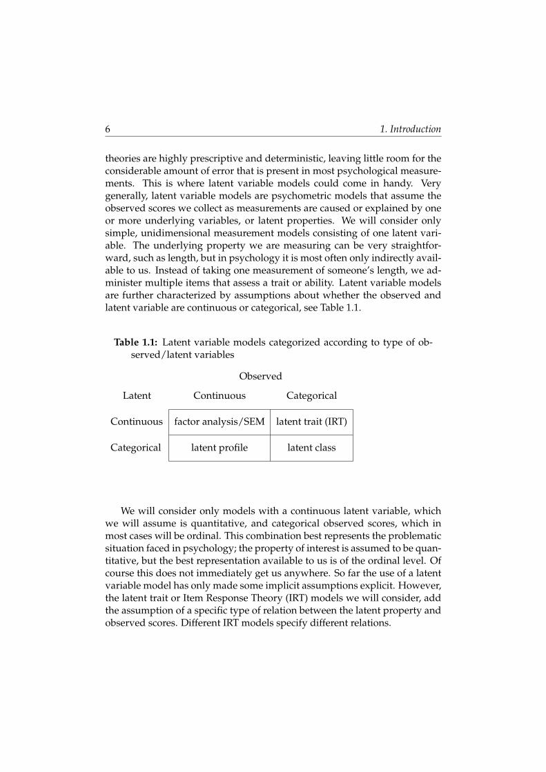
theories are highly prescriptive and deterministic, leaving little room for theconsiderable amount of error that is present in most psychological measure-ments. This is where latent variable models could come in handy. Verygenerally, latent variable models are psychometric models that assume theobserved scores we collect as measurements are caused or explained by oneor more underlying variables, or latent properties. We will consider onlysimple, unidimensional measurement models consisting of one latent vari-able. The underlying property we are measuring can be very straightfor-ward, such as length, but in psychology it is most often only indirectly avail-able to us. Instead of taking one measurement of someone’s length, we ad-minister multiple items that assess a trait or ability. Latent variable modelsare further characterized by assumptions about whether the observed andlatent variable are continuous or categorical, see Table 1.1.
Table 1.1: Latent variable models categorized according to type of ob-served/latent variables
Observed
Latent Continuous Categorical
Continuous factor analysis/SEM latent trait (IRT)
Categorical latent profile latent class
We will consider only models with a continuous latent variable, whichwe will assume is quantitative, and categorical observed scores, which inmost cases will be ordinal. This combination best represents the problematicsituation faced in psychology; the property of interest is assumed to be quan-titative, but the best representation available to us is of the ordinal level. Ofcourse this does not immediately get us anywhere. So far the use of a latentvariable model has only made some implicit assumptions explicit. However,the latent trait or Item Response Theory (IRT) models we will consider, addthe assumption of a specific type of relation between the latent property andobserved scores. Different IRT models specify different relations.
1.5. Overview 7
The general question that formed the motivation for this thesis is howwe should deal with the problem of admissible statistics and legitimate in-ference from a latent variable perspective. The concept of admissible statis-tics entails a very strict limitation on the tests that we can perform on datathat were modeled with a latent variable model. Whether this prescriptionshould be given heed or whether assumptions or other characteristics of la-tent variable models protect us from making illegitimate inferences is an im-portant topic, especially since psychometrics has been under increased at-tack recently from critics who maintain that psychometrics is shirking itsresponsibility to actively inquire into the quantitative status of psycholog-ical measurement (Michell, 1986, 1997, 2008a, 2008b, 2009). Perhaps latentvariable models can be used to lay bare this elusive quantitative structurein more psychological properties or assist in the answering of measurementlevel questions in other, more indirect ways.
1.5 Overview
In this thesis the feasibility of legitimate inference and the assessment of mea-surement level for psychological properties is discussed from a latent vari-able perspective. The three chapters following this introduction are devotedto several theoretical problems associated with admissible statistics and le-gitimate inference. The first chapter deals with arguments against the restric-tions that admissible statistics pose. In the second and third chapter a latentvariable model is addressed that is claimed to ensure legitimate inference.There are several conceptual problems that surround this claim. The finaltwo chapters concern a more practical approach. In both chapters a simu-lation study is presented that assesses the risk of inferential error. Differentlatent variable models were used to generate the simulated data.
In Chapter 2 the origins of the measurement-statistics debate are dis-cussed. The argument that statistics should not be governed by measure-ment level considerations is critically evaluated. The focus of the chapter ison a thought experiment by Lord (1953) that for a large part set off and per-petuated this debate. The thought experiment concerns a fictional professorwho feels guilty performing inadmissible tests on his students’ ordinal examscores. He suffers a breakdown and retires early. In his new job, selling jer-sey numbers to the football teams, an altercation between two teams arises.

8 1. Introduction
One team complains that they received lower numbers due to tampering bythe other team. A statistician settles the matter by performing a t-test on themean of the numbers. Although this test is inadmissible, since the numbersare of the nominal level, only distinguishing players on the field, the con-clusion seems useful and somehow meaningful. A critical evaluation of thisthought experiment shows however, that the parable can be reinterpreted sothat it is perfectly in line with the rationale behind the concept of legitimateinference. A latent variable perspective is used to identify the underlyingproperty of interest and a representational approach is used to show thatthis property can be represented at the interval level. This analysis showsnot only that the most influential argument against inadmissible statisticsis flawed and that application of only admissible statistics seems justified,but also that measurement level considerations are more complex than wegenerally think.
The property of bias in a number-issuing machine in Lord’s thought ex-periment is not a very interesting one from a psychological point of view. Formost properties that are of interest to psychology, interval level measurementis unattainable. There are circumstances however where such measurementis possibly within reach. These circumstances are captured by the assump-tions of the well-known Rasch Model. This model, according to many, is aninstantiation of an additive conjoint representational measurement structure.This is a structure for which it was shown (Luce & Tukey, 1964) that if its ax-ioms hold, the representation is of the interval level. This is a potentiallyimportant foothold for psychology. If the Rasch model can provide us with amethod to attain interval level measurement then for at least some propertieslegitimate inference will no longer be a problem. The claim that the Raschmodel ensures interval level measurement is not uniformly accepted how-ever. In Chapter 3 general problems of combining the latent variable model-ing perspective with representational measurement in general and the Raschmodel in particular are examined concerning the interpretation of probabil-ities, the spatio-temporal status of model parameters and the finite and in-herently discrete nature of many psychological properties.
Unfortunately these are not the only problems with the interval levelclaim associated with the Rasch model. Another issue concerns a paradoxwe call the Guttman-Rasch paradox. This paradox consists of a counter-intuitive difference in measurement level between the Guttman and Raschmodel. Both models are IRT models that describe the probability of answer-

1.5. Overview 9
ing an item correctly as a function of the difference of the person ability anditem difficulty. The Guttman model is deterministic and states that this prob-ability is 0 if the ability is lower than the item difficulty and 1 if it is higher.The Rasch model is probabilistic and specifies the probability as a logisticfunction of the difference between person and item. The Rasch model can beconsidered an extension of the Guttman model that arises from the additionof error by assuming a monotonically increasing relation between probabil-ity correct and the latent trait. Now, the Guttman model, which contains noerror, allows ordering of items and persons. In contrast, the Rasch model,which does contain error, allows interval level measurement. Introductionof error is therefore associated with an increase in measurement level. Thisparadoxical situation is discussed in Chapter 4, where it is shown that al-though an increase due to error is counter-intuitive, it is not paradoxical perse. Since the error in the Rasch model is dependent on the difference betweenitem and person, it is in fact informative about the latent trait. In physics andbiology this phenomenon is known as stochastic resonance.
Latent variable models can also be incorporated to investigate admissi-ble statistics in a very different way. They are employed to assess the actualrisk of obtaining ambiguous or distorted results when an inadmissible test isperformed. One type of research effect for which inadmissible tests can leadto distorted results, or inference errors, is the interaction effect. Latent vari-able modeling can be used to make specific assumptions about the relationbetween ordinal observed scores and the assumed underlying quantitativevariable. In Chapter 5 several types of interaction effects were simulatedaccording to the two-parameter logistic IRT model (2PL). An experimentalsetting was simulated by using a fixed-effects, small sample two-by-two de-sign. Results showed that inferential errors occur when the test is ill-matchedin difficulty to the ability of the sample. If a test is too hard, floor effects occurthat result in unequal stretching of the observed scale, due to the nonlinearrelation that the 2PL model specifies. Inference errors only occur howeverwhen test discrimination is high and only for certain types of interaction ef-fects. The risk of inferential error therefore seems limited to very special cir-cumstances. Moreover, in these specific circumstances, inferential error canbe mitigated to some extent by performing a normalizing transformation onthe observed scores.
In Chapter 6 an extension of this simulation study is presented. The samesimulation was performed, but this time the Graded Response Model (GRM)
10 1. Introduction
was used to transform latent values into observed scores. The GRM modelsitem responses for items that have multiple ordered response categories. Be-sides the match between test difficulty and item ability, other factors such asitem discrimination, effect size, type of effect and number of response cate-gories was investigated. Results were comparable but much less severe forthe data that was generated using the polytomous GRM model comparedto the binary 2PL model. The risk of inferential error clearly decreased asthe number of response categories increased. A normalizing transformationwas also more effective in mitigating the risk of inferential error. These re-sults support the conclusion that inadmissible statistics pose a real threat toour inferences. Only if a test is extremely hard or easy, and only then if theitems also discriminate strongly and if certain interaction effects occur.
A summary and discussion of both the theoretical (Chapters 2, 3 and4) and more practical (Chapters 5 and 6) treatment of admissible statisticsis provided in Chapter 7. Here it will be argued that the prescriptive re-quirement of axiom testing advanced by representationalists as well as theirfiercest critics, the traditionalists, is not a fruitful strategy to further scientificknowledge of the structure of psychological properties. The properties thatare even remotely amenable to such rigid methods are scarce and the avail-able methods themselves are ill-equipped to deal with psychology’s error-laden properties. Psychological researchers would do well to be a bit moreconservative in their inferences and use of the word measurement when themeasurement status of their observed data is dodgy at best. This is not tosay that psychology should no longer be considered a science. The fact thatpsychology deals with a much more elusive subject matter than physics doesnot mean we should give up at the outset. It is important to realize however,that this is where psychology as a quantitative science still finds itself. Weare a nascent quantitative field, not an established one.

Chapter 2
A Reanalysis of Lord’s Statistical Treatment ofFootball Numbers
‘I checked it very thoroughly,’ said the computer, ‘andthat quite definitely is the answer. I think the problem,to be quite honest with you, is that you’ve neveractually known what the question is.’
Douglas Adams - The Hitchhiker’s Guide to theGalaxy
Abstract
Stevens’ theory of admissible statistics (1946) states that measurement lev-els should guide the choice of statistical test, such that the truth value ofstatements based on a statistical analysis remains invariant under admissibletransformations of the data. Lord (1953) challenged this theory. In a thoughtexperiment, a t-test is performed on football numbers (identifying players: anominal representation) to decide whether a sample from the machine issuingthese numbers should be considered non-random. This is an inadmissible test,since its outcomes are not invariant under admissible transformations for thenominal measurement level. Nevertheless, it results in a sensible conclusion:the number-issuing machine was tampered with. The present aim is to showthat the thought experiment contains a serious flaw. First, the assumptionthat the numbers are nominal is shown to be false. Second, it is argued that thefootball numbers represent the amount of bias in the machine. The level of biasin the machine, indicated by the population mean, conforms to a bisymmetricstructure, which means that it lies on an interval scale. In this light, Lord’sthought experiment interpreted by many as a problematic counterexample toStevens’ theory of admissible statistics conforms perfectly to Stevens’ dictum.

12 2. A Reanalysis of Lord’s Statistical Treatment of Football Numbers
2.1 Admissible Statistics
In a typical introductory statistics class, psychology students are taught thatthe level of measurement should be taken into account when choosing a
statistical test. For example, a t-test should not be performed on data thatare of a nominal or ordinal level. Exactly why this rule should be followedis rarely explained and not widely known among psychologists; thereforethe rationale for it is reiterated. Suppose mathematical proficiency of chil-dren was measured on an ordinal level. In such a case, one is justified intransforming the data by taking the square for example, because the ordi-nal property in the data, the original ordering of the children, is preserved.For an ordinally measured property, all monotonically increasing, or order-preserving transformations of the data are completely equivalent in theirrepresentational capacities, i.e. they all represent the measured propertyequally well. In fact, in measurement theory this is the defining feature ofscale levels (Krantz, Luce, Suppes, & Tversky, 1971).
With respect to the results of parametric statistical analyses that may beexecuted on the differently transformed data, however, no such equivalenceexists. For instance, it is possible that when scores on the aforementionedmathematical proficiency test are analyzed for sex differences with a t-test,different results are obtained for the original and transformed scores. Boysmay significantly outperform girls when analyzing the original scores, whileboys and girls may not differ significantly in their performance when ana-lyzing the transformed scores (or vice versa; see Hand, 2004, for some in-teresting examples). Since there is no sense in which the original scores arepreferable or superior to the transformed, squared scores, this means thatresearch findings and conclusions depend on arbitrary, and usually implicit,scaling decisions on part of the researcher. This hinders scientific progressbecause it obscures a factor, namely the choice of scaling, that is influen-tial in determining conclusions based on empirical research. It is important,therefore, to have a clear understanding of how level of measurement canaffect our conclusions.
Stevens (1946) introduced the concept of measurement levels and rulesfor choosing a statistical test according to the dependent variable’s measure-ment level in order to prevent arbitrary scaling decisions from affecting re-search outcomes. His theory has become known as the theory of admissi-

2.1. Admissible Statistics 13
ble statistics (e.g., Robinson, 1965). The basic idea is that one should onlyperform statistical tests that yield conclusions that are invariant under all so-called ‘admissible transformations’ (admissible in the purely technical andnon-pejorative sense of having the same representational capacities) of thedata. These admissible transformations are one-to-one transformations fornominal data, order-preserving transformations for ordinal data, positivelinear transformations for interval data and transformations that multiplywith a positive constant for ratio data (see Krantz et al., 1971; Suppes &Zinnes, 1963). Using admissible statistics ensures that conclusions about themeasured property are not dependent on numerical values arbitrarily chosento encode the data. Thus, in respecting the measurement level, one removesa threat to the validity of the conclusions, which is a good thing.
2.1.1 The Measurement-Statistics Debate
On first sight, one may expect this simple fact to be universally appreciatedas a powerful insight into the relation between measurement and statistics.Therefore, it may be considered surprising that the concept was not uni-formly welcomed by statisticians, some of whom vehemently rejected thesuggestion that measurement levels could have any bearing on data analy-sis. Several arguments have been adduced in support of this view. Some ar-gue that the level of measurement is often very hard to determine. Vellemanand Wilkinson (1993) maintain that in real situations, data do not always fallneatly into the scale levels describes by Stevens (1946), which is problematicwhen applying his rules. Others have argued that theoretically inadmissiblestatistics can be arbitrary, but that in practice they rarely are (Baker, Hardyck,& Petrinovich, 1966). That is, inadmissible parametric statistics tend to agreewith their more cumbersome admissible counterparts, so that real harm israrely done by executing statistical analyses that are strictly inappropriate.
These arguments against the idea of admissible statistics are pragmatic incharacter (i.e., determining the level of measurement is too hard, parametricanalyses are easier to use, etc.). Hence it may seem as if substantial agree-ment exists among scholars regarding the general validity of Stevens’ ideas,even if adhering to this idea is not generally advisable. This is not the case,however. Some are of the opinion that there is a principled problem withStevens’ view and think that there exists no connection between the levels ofmeasurement and the validity of results attained through statistical analyses
14 2. A Reanalysis of Lord’s Statistical Treatment of Football Numbers
at all. Statistical tests simply help the researcher to decide whether their data– in the form of a set of numbers – is likely to be a random sample drawnfrom a larger population of numbers having a specific distribution. Whatthe numbers measure is irrelevant to this particular decision, and hence is-sues concerning the level of measurement are irrelevant as well (Burke, 1953;Gaito, 1980).
2.1.2 Lord’s Controversial Argument
One of the most important arguments supporting this ‘statistical’ perspec-tive was provided by Lord (1953). He is uniformly cited among opponentsof the theory of admissible statistics (Gaito, 1960; Anderson, 1961; Baker etal., 1966; Gaito, 1980; Velleman & Wilkinson, 1993; Kampen & Swyngedouw,2000; Harwell & Gatti, 2002; Pell, 2005). Lord introduces a thought experi-ment in which the use of an inadmissible parametric test on nominal num-bers leads to a legitimate, useful and seemingly non-arbitrary conclusion.Lord thus appears to present a clear counterexample to Stevens’ theory ofadmissible statistics. In doing so, he lends support to the view that levels ofmeasurement should not influence one’s choice of statistical analysis. Lord’sargument sparked what is now called the measurement-statistics debate, andmust be considered the most influential and certainly the most entertainingcritique of the theory of admissible statistics to date. As such, the two-pageletter about a nutty statistics professor has become something of a locus clas-sicus in the literature on psychological measurement and statistics.
Notwithstanding its rhetoric force, Lord’s contribution was severely crit-icized. Some responded by clarifying the basic principles of Stevens theory,giving examples where computations on nominal data lead to absurd con-clusions (Behan & Behan, 1954; Bennet, 1954; Stine, 1989). Others pointedout that although computations can be performed on a nominal variable, theresults have no reference to the empirical world and so they are irrelevant(Townsend & Ashby, 1984). In our view, however, most of the publishedcriticisms have not gotten to the heart of the matter, in that they fail to ex-plain why the conclusion in Lord’s thought experiment is useful, while at thesame time the statistical test is inadmissible.
The goal here is to unravel this problem, and to show that Lord’s thoughtexperiment does not provide a valid counterexample to Stevens’ theory of

2.2. The Treatment of Football Numbers 15
admissible statistics. We start by revisiting Lord’s thought experiment indetail. After analyzing an important, but implicit assumption, it is arguedthat the validity of the thought experiment hinges on the question of whatproperty the numbers represent in relation to the statistical question that isasked. It is then shown that in relation to this statistical question, the num-bers clearly do not represent a nominal property.
This conclusion is enough to disqualify Lord’s thought experiment as avalid counterexample to Stevens’ theory. Additionally however, it is pos-sible to identify a property that actually is relevant to the statistical ques-tion. The structure of this property and its measurement level is explored.It is argued that the data can represent this newly identified property on aninterval level, which provides a genuinely new outlook on Lord’s thoughtexperiment. For in this new light, Lord’s thought experiment is not a coun-terexample, but instead a perfect illustration of Stevens’ theory of admissi-ble statistics. Related arguments made by critics of the theory of admissi-ble statistics are addressed, and it is argued that statistics and measurementcannot be viewed separately when one wants to make meaningful inferencesabout the properties that one intends to measure. Finally, ways are discussedin which researchers can deal with the implications of our discussion of Lordand incorporate decisions about measurement levels in their research.
2.2 The Treatment of Football Numbers
2.2.1 The Nutty Professor
Lord (1953) describes a university professor who loves to compute meansand standard deviations of his students’ grades, which measure proficiencyon an ordinal level only. He knows this is against Stevens’ rules and he feelsso guilty that he goes into early retirement. Instead of a gold watch, the uni-versity gives him an enormous amount (a hundred quadrillion) of two-digitcloth numbers and a vending machine. He can sell these numbers to thefootball teams, so they can use the numbers to distinguish players on thefield. In somewhat oblique terms, one could say that the numbers ‘measure’the uniqueness of the players, obviously on a nominal level. After makingan inventory of the numbers, the professor shuffles them, puts them in thevending machine, and sells a large pile of numbers (1600 to be exact), first

16 2. A Reanalysis of Lord’s Statistical Treatment of Football Numbers
to the sophomore team and then to the freshman team. After a few days thefreshmen come back with a complaint. The sophomores have been makingfun of them for having received lower numbers. The professor now facesa problem: The freshmen receiving lower numbers could be either a coinci-dence or the result of foul play. The professor decides to ask a statistician forhelp.
The statistician computes means and standard deviations for the popula-tion and the freshmen sample, computes a critical ratio test statistic, whichis essentially a one group t-test comparing the sample mean to the popula-tion mean using the population standard deviation. He then applies Cheby-shev’s inequality (since the population is not normally distributed) and findsa very small p value. The professor of course protests heavily that such a testis inadmissible for a variable measured on a nominal level. The statisticianresponds by challenging him to draw new samples from the vending ma-chine and to see how many times he finds a mean equal to, or lower thanthe freshman mean. The professor does so many times and finds only twosuch values. He is now satisfied that the machine was tampered with andprovides the freshmen with new numbers. He is so heartened by this mean-ingful use of a parametric test on a variable measured on a nominal level,that he decides to come out of retirement.
2.2.2 The Implicit Argument
The covert moral in this parable seems to be that Stevens’ theory of admis-sible statistics is incorrect, because the argument provides a counterexamplewhere an inadmissible test leads to a meaningful result. But does this conclu-sion necessarily follow from Lord’s thought experiment? A more structuredapproach may clarify this issue. The implicit argument Lord makes can berepresented by a logical statement about two propositions:
• P1: performing interval manipulations on data that represent mea-surement on the nominal level results in a meaningless conclusion (i.e.Stevens’ theory of admissible statistics is valid);
• P2: performing a parametric test on the football numbers results in ameaningless conclusion.
2.2. The Treatment of Football Numbers 17
The logical statement is: if P1, then P2; If Stevens’ theory of admissiblestatistics is valid, then what Lord’s statistician does, results in a meaning-less conclusion. But the results are not meaningless, for they lead to a usefulconclusion; based upon the results of the test, it is concluded that the ma-chine was tampered with and decided that the freshmen should receive newnumbers. So, P2 is false, which, by modus tollens, entails that P1 is false;since performing a parametric test in this situation is sensible, performinginadmissible statistical tests on data must be justified, at least in some in-stances. Lord’s parable thus leads the reader to the conclusion that levels ofmeasurement are not always relevant to the choice of statistics.
The above representation, however, does not paint a full picture of Lord’sthought experiment. There is an implicit assumption concerning the mea-surement level of the football numbers that is not included as a proposition.Lord’s parable is better represented by making this assumption explicit:
• P1a: performing interval manipulations on data that represent mea-surement on the nominal level results in a meaningless conclusion (i.e.Stevens’ theory of admissible statistics is valid);
• P1b: the football numbers measure a property on the nominal level;
• P2: performing a parametric test on the football numbers results in ameaningless conclusion.
The logical statement now becomes: if P1a and P1b, then P2; if Stevens’ the-ory of admissible statistics is valid and the football numbers measure a prop-erty on the nominal level, then what the statistician does is nonsensical. Itnow becomes clear that the reason that P2 does not hold could lie elsewhere.If P2 is false, either P1a, or P1b, or both, must be false. P1b is not questionedin Lord’s parable; the football numbers obviously measure a property on thenominal level. But is it really so obvious that the relevant property in Lord’sthought experiment is a property on a nominal scale? If it can be shown thatP1b is false, then P1a, and with it the theory of admissible statistics, does nothave to be rejected.
18 2. A Reanalysis of Lord’s Statistical Treatment of Football Numbers
2.2.3 What Do the Football Numbers Measure?
The professor in Lord’s thought experiment repeatedly emphasizes that thenumbers are nominal representations of the uniqueness of the players. Now,the numbers can certainly be used to distinguish players on the field; but thisis not the property for which the statistician uses the numbers. Instead, theprofessor asks a question and draws a conclusion about the machine, namelythat it was unlikely to be in its original state (randomly shuffled by the pro-fessor) when the freshman numbers were issued. Thus, while an informativeinference to the state of the world has been made, this inference does not con-cern the uniqueness of the football players at all. The level of measurementthat the numbers have with respect to these players is completely irrelevantto the thought experiment. Since the players are where the numbers get theirstatus as nominal measurements from, a further conclusion must be drawn:whether a nominal level of measurement plays any role at all in the argu-ment is as yet unsubstantiated. For this reason, premise P1a cannot figure inthe argument as described by Lord.
It is prudent to note that we are not the first to point out that the profes-sor’s conclusion does not pertain to the football players. Several of Lord’scritics have argued this point (Behan & Behan, 1954; Bennet, 1954). Theyemphasize that Stevens’ rules of admissible statistics presuppose that thestatistics are performed on measurements of some empirical property, andmaintain that the numbers as they are used in the test do not represent anysuch property; hence Lord’s parable does not provide a counterexample torefute Stevens’ dictum. Adams, Fagot, and Robinson (1965, p. 125 ) actu-ally state: “In other words, the hypothesis is concerned with the method ofassigning numbers, and has nothing to do with any hypotheses about mea-surable properties of objects”. Unfortunately, these critics fail to note thatwhile the numbers do not refer to the football players in any relevant way,they may refer to another property that is relevant, i.e., the degree to whichthe machine is biased.
This observation puts us back at square one, for the basic premise thatshould support Lord’s logical construction and the many papers that haveused it to substantiate arguments against the theory of admissible statis-tics is left in doubt. The relevance of Lord’s argument to Stevens’ theoryis no longer obvious. The property that fosters measurement level claims(uniqueness of players) and the property that the statistical conclusion refers
2.3. Vending Machine Bias 19
to (state of the machine) should be one and the same. This is plainly notthe case in Lord’s parable. Treatment of Lord’s parable could cease here,since this conclusion alone is enough to disqualify the thought experimentas a counterexample to Stevens’ dictum. However, the intriguing questionwhy the conclusion based on the parametric test seems so sensible remainsunanswered. Perhaps Lord’s story about the nutty professor does have somerelevance to Stevens’ theory, but in a way different from how it is generallyviewed. To evaluate such relevance if there is any we need to reconsider thebasic question what the football numbers measure and, especially, what theassociated level of measurement may be.
It could be argued that, since the statistician performs a one-sample t-testwith a fixed population mean, the results will not be invariant under anytransformation of the data, so that the statistician is actually assuming an ab-solute scale. However, in such a line of reasoning one attempts to ascertainthe measurement level of the data by looking at the invariance of statisticalresults, which is not in line with the representational measurement literatureor Stevens’ dictum. Establishing a measurement level implies the invarianceof statistical tests with respect to the class of admissible transformations, butthe reverse is not necessarily true: the invariance of statistical tests with re-spect to a class of admissible transformations does not imply a measurementlevel. Otherwise one could infer that one has interval level measurementsfrom the fact that the results of a t-test are invariant under linear transforma-tions of the data; this is clearly not the case, because the results of a t-test arealways invariant under linear transformations of the data, whether these areat the interval level or not.
2.3 Vending Machine Bias
Lord’s statistician uses the statistical results to make an inference about thestate of the vending machine, and decides that the freshman mean did notcome from the machine in its original state. Thus, Lord’s inference concernsthe state of the machine relative to another (possible) state of the machine.His reference class is not a set of football players, but a set of possible statesof the machine (e.g., fair and biased states). Insofar as measurement is tak-ing place in the thought experiment, therefore, it relates to the assignment

20 2. A Reanalysis of Lord’s Statistical Treatment of Football Numbers
of a label to the machine. And in this regard, Lord’s example is in perfectaccordance with Stevens’ theory of admissible statistics.
To see this, it is necessary to first consider how the machine came to bein its altered condition. If we have a better idea what we mean by the stateof the machine, better insight may be developed into the nature of the infer-ence being made. Lord gives us a clue how the state of the machine couldhave been altered by hinting that the professor suspects foul play by thesophomores. Now, the sophomores could have tampered with the machinein several ways. For example, the vending machine could be imagined as anenormous stacked pile of numbers. The numbers are issued one by one fromthe top of the stack. The sophomores could have tampered with the vendingmachine by replacing or removing specific numbers at the top of the stack.This way they could ensure that the freshmen received an inordinate amountof even numbers, or numbers ranging from 20 to 30, or prime numbers; thepossibilities are endless.
2.3.1 Nominal Bias
If we do not make any assumptions about the way in which the machinewas tampered with, the question posed to the statistician may be reformu-lated into the following research hypothesis: is the machine tampered withor not? This state of tampering can be conceived of as a property of the ma-chine that can be represented nominally with two distinct categories: tam-pered with and not tampered with. However, it is clear that this way ofthinking about Lord’s method is in poor accordance with the statistical pro-cedure utilized. That is, if the question were merely “was the machine tam-pered with or not?”, then the test that the statistician performs is not a verygood one. It is possible, for instance, that the sophomores removed all thenumbers from 01 to 30 and from 70 to 99. The machine would, in this case,clearly be tampered with, but the expected sample mean would not be dif-ferent from the population mean in the long run. The tampering would notshow up in a test were the mean is used to detect a deviation in the samplefrom the population; the sensitivity of the assignment procedure would bevery low.

2.3. Vending Machine Bias 21
2.3.2 Ordinal Bias
Now consider the fact that Lord provided the statistician with a good argu-ment to use the mean to discover any tampering. The freshmen do not justcomplain that their sample is different from the expected population, butthat the numbers are lower. The freshmen’s distaste for low numbers doesnot magically imbue the numbers with a higher level of measurement, ofcourse, but it does give us more information on how the machine was tam-pered with. This enables us to refine our understanding of the property ofthe machine that we are interested in. Knowing that low numbers wouldupset the freshmen could have prompted the sophomores to remove highnumbers from the top of the stack of numbers in the machine. If we focuson this specific type of tampering we can say not only whether the machinewas tampered with or not, we can now also say whether the machine wastampered with to a greater or lesser extent. Bias can be introduced into themachine (still consisting of a stack of shuffled numbers) by replacing highnumbers with low numbers (or vice versa), resulting in a lower (or higher)population mean. The tampering method suspected by Lord’s professor andtested in the statistical analysis is clearly one that introduces a bias towardlower numbers. The sophomores could have been very subtle and removedonly a few high numbers, or they could have been extremely overt in theirmischief and removed all the numbers larger than 10. The more consistentlythis replacement is performed, the more bias will be present.
More formally, the amount of bias can be thought of as a variable byimagining a population of vending machines with varying amounts of bias.This idea is illustrated in the right panel in Figure 2.1 by machine 1 to n,which is a subset of the total conceivable population of machines, in whichevery amount of bias possible is present. The amount of bias in the machinecan be represented pragmatically by taking the population mean of the num-bers as an indicator for the ordering of the locations of the distributions inquestion, or by using a nonparametric concept such as stochastic orderingfor this purpose. The mean of the extracted numbers may then be comparedto the population mean of a fair machine. If there is no bias, the expectedvalue of the sample mean is expected to be equal to this population mean.
To compare this point of view to Lord’s sketch of the situation, considerthe left panel in Figure 2.1. The property of uniqueness or non-identity ofthe players is denoted by the relational symbol 6≈. This property is repre-

22 2. A Reanalysis of Lord’s Statistical Treatment of Football Numbers
Figure 2.1: Graphical representation of measurement on the nominallevel of the uniqueness of the football players (left panel) and mea-surement on the interval level of the bias in n vending machines(right panel)
� ��
� ��� � � … �
������������� �� ��� � �� ��� A� �B �C ��� �A
� ��… ����DEF���� DEF������ DEF����� DEF������
��Measurement on the nominal level of uniqueness of the players, the vending machine is irrelevant.
: Measurement on the interval level of bias in the conceptual machines, the players are irrelevant.
: Indicates correspondence of empirical ( ,� �) relations between objects on the attribute of interest on one hand, and numerical ( ≠ , < ) relations between numbers on the other hand.
��
: The mean of machine n.
������
�����
����
sented by using different numbers to represent unique players, denoted inthe figure by the symbol 6=. In the right panel of Figure 2.1, bias in a machineis represented by a mean, in the same way a football player’s uniquenessis represented by a single football number. Clearly, the players can only bejudged to be different from one another. Equally clearly however, the ma-chines are not merely different from one another; they can also be orderedaccording to the amount of bias they possess. Normally, relations betweenobjects on the empirical level are described in qualitative terms and thenthe numbers come in to represent these relations on the numerical level. Itmight seem a bit strange that in our case the objects on the empirical levelalready consist of numbers, but this is the nature of the vending machine asconstructed by Lord. That is, the numbers in the machine are numbers, notrepresentations, and therefore relations between these numbers can be used(in this case by the sophomores) to make up empirical relational systems thatare subsequently represented by a separate numerical relational system.
2.3. Vending Machine Bias 23
2.3.3 Interval Bias
It is clear that such an empirical relational system can be constructed, andthat Lord’s measurement problem involves at least an ordinal structure atthe level of the machine. However, it appears that more structure than mereorder can be established in the property of bias; one suspects, in fact, that thisstructure is quantitative in the sense that it should be meaningful to say thatthe difference in bias between two machines is equal to the difference in biasbetween two other machines. It turns out that it is possible to show that thebias in the machines has quantitative structure and that the number that thestatistician uses to represent it (i.e., the mean) is actually an interval measureof this structure. To this purpose, we need to show that additive structure ispresent in our bias property and that this structure is represented uniquelyup to linear transformations by the population mean.
To show that the machines’ level of bias towards low numbers possessesquantitative structure, it suffices to show that an operation exists that al-lows us to concatenate machines, and that the resulting concatenation hasthe right properties (Krantz et al., 1971). The operation proposed here veryloosely follows the analogy of concatenating temperatures in volumes of liq-uid. Two equal volumes of liquid, each of a particular temperature, can beadded to each other. The resulting temperature is the mean of the separatetemperatures. A similar operation on the machines can be conceptualized;the bias in two machines could be ‘added’ by concatenating the numbersdrawn from each machine into a new randomly shuffled pile, which func-tions as the concatenation of the original machines. This operation allowsfor the establishment of a relation that satisfies the requirements for mea-surement on an interval level. The operation is based on the representationalmeasurement theorems describing bisymmetric structures by Krantz et al.(1971, p. 294), which were developed for mean structures. A formal treat-ment of the bisymmetric structure and how it applies to Lord’s thought ex-periment is provided in Appendix A. That the operation results in measure-ment on an interval level is intuitively clear. Any non-linear transformationwould stretch or shrink the scale somewhere and make comparison of dif-ferences in bias of machines impossible. Any linear transformation however,would represent the bias towards low numbers in these machines equallywell.

24 2. A Reanalysis of Lord’s Statistical Treatment of Football Numbers
It was already shown that Lord’s parable does not provide a counterex-ample to Stevens’ dictum, because the assumption that the numbers are ona nominal level is invalid. No further analysis of Lord’s thought experimentis needed to make this point. However, when we do take a closer look at itsstructure, it is clear that there exists at least one conceptualization of Lord’sthought experiment in which the statistician is operating in accordance withStevens’ principles. Therefore, in addition we have now shown that the pro-cedure followed can actually be viewed as an illustration of the theory ofadmissible statistics. Viewing Lord’s thought experiment in this way alsoanswers the question why the statistician’s conclusion seems so sensible. Itis sensible because it is about a relevant property of the machine.
2.4 Conclusion
We have examined extensively why the test in Lord’s thought experimentappears to be inadmissible, while at the same time it leads to a scientificallyuseful and informative conclusion. In doing so Lord’s argument was foundto depend on the assumption that the football numbers represent a prop-erty on the nominal level. Not only was it shown that it is immaterial tothe argument that the numbers represent nominal uniqueness of the players,it was also possible to identify another relevant property, namely the levelof bias towards low numbers that a machine exhibits. The numbers in factrepresent both the property of uniqueness (in relation to the players) on anominal level and the property of bias (in relation to machines) on an inter-val level. What is important here is that the property that corresponds tothe statistical question must be considered in determining the admissibilityof a test. Because the freshmen complain about low numbers and becausethe statistician uses a test of the mean that is sensitive to order and differ-ences we conclude that Lord’s professor was actually interested in inferringsomething about bias in the machine towards low numbers. This propertyof bias was argued to have a structure that can be measured on an intervalscale by the population mean, thereby transforming Lord’s counterexampleinto a perfect illustration of Stevens’ theory of admissible statistics.
2.4. Conclusion 25
2.4.1 Representing Several Properties at Once
Our analysis relies on the assumption that a single set of numbers may havemultiple representational purposes. It is interesting, in this respect, that someof Stevens’ critics have used the fact that the same data can represent differ-ent properties as an argument against Stevens’ theory of admissible statistics.Velleman and Wilkinson (1993), for instance, argue that the level of measure-ment is not a characteristic of the data. They state that the same numbers canrelate to different properties at different measurement levels. Why this is anargument against Stevens might (and should) seem oblique to the reader. Itwas probably incited by Stevens’ procedure for determining the level mea-surement by assessing the rule used to assign numbers.
In Stevens’ thinking, a property can be represented on an interval level ifparticipants can judge intervals on this property to be equal. The rule used toassign numbers thereby determines the measurement level for these partic-ular numbers; once a rule is chosen, the measurement level is set. However,even in Stevens’ original papers, one can identify appeals to the requirementthat the rules used to assign numbers must yield a numerical structure thatis isomorphic to that of the property measured, or to its behavior under em-pirical operations (Stevens, 1946, p. 677). In a more sophisticated form, thisrequirement became a cornerstone of representational measurement theory.When one accepts that representational measurement theory has replacedStevens’ original, rather crude theory of levels of measurement, Vellemanand Wilkinson’s point becomes moot. In representational measurement the-ory, the level of measurement is determined jointly by the structure of theproperty of interest and the relation that the numerical assignments bear tothat structure. According to this view, nothing prevents the same numbersfrom representing different aspects of a property, or different properties al-together.
2.4.2 Lord’s Forgotten Rejoinder
[h] Reflection on Lord’s thought experiment and the critique by Vellemanand Wilkinson (1993) nicely illustrates that what our numbers and our con-clusions refer to is not always as obvious as we may think. The fact that asimple football number example still puzzles us after more than fifty yearsshows that measurement issues in relation to legitimate inference (a term

26 2. A Reanalysis of Lord’s Statistical Treatment of Football Numbers
coined by Michell, 1986) concerning a measured property deserve our atten-tion. Researchers should be aware of the inferential power of their statisticalconclusions or the lack thereof. Perhaps surprisingly, Lord would probablyhave agreed. In a response to his critics, published a year after the originalarticle (Lord, 1954), he stated that when one wants to draw an unambiguousconclusion about a property that at best can be represented ordinally, inde-pendent of the scale that was used, then nonparametric statistics should beemployed.
The point Lord ostensibly intended to make is that Stevens’ rules shouldnot be applied mindlessly when choosing a statistical test, but that each sit-uation should be considered anew. In the football numbers argument, Lordattempted to show that there are situations conceivable where these rulesdo not have to be applied. In all likelihood, however, Lord did not recog-nize that a relevant property allowing interval level representation could beidentified in his example. Had Lord recognized that the football numbersrepresent the property of bias in the machine on an interval level, he proba-bly would have agreed that his thought experiment does not provide a com-pelling argument against Stevens’ ideas. It remains to be seen if anyone isable to come up with an example where a question about a nominally mea-sured property, answered with a parametric test, results in a truly sensibleconclusion about the same nominal property that the numbers refer to. Thischallenge, of course, stands for all those who argue that statistics and mea-surement are completely disconnected scientific domains.
2.4.3 Determining the Level of Measurement
Unfortunately, Lord’s first publication (1953) has had an enormous influenceon the measurement statistics debate; nearly every contributing author refersto this publication. All of Stevens’ opponents use Lord’s thought experimentand the infamous quote1 “the numbers don’t know where they came from”(Lord, 1953, p. 751) to illustrate their arguments, sometimes even using thequote itself as an argument (Gaito, 1980, p. 565). In contrast, his follow-uppublication (1954) has been cited only three times (web of science citationsearch, at the time of publication). This is regrettable, because Lord’s in-
1The text actually reads: “The numbers don’t know that. Since the numbers don’t remem-ber where they came from, they behave just the same way, regardless.”
2.4. Conclusion 27
tended point was right on the money: Stevens’ rules should not be appliedmindlessly.
Careful deliberation is necessary, because one can easily lose sight of thecorrespondence between the property that is actually being measured andthe property about which one wants to make an inference. When choos-ing a statistical test, considerable thought should be given to the propertyabout which one wants to draw a conclusion, the way this property is mea-sured, and the level it is measured on. Of course, drawing firm conclu-sions about the achieved measurement level is almost always beyond ourreach (see Roberts, 1986, on how the theory of meaningfulness can be ap-plied in psychology). Demanding that the level of measurement for psycho-logical properties is unequivocally determined before continuing with sub-stantive research would bring psychological inquiry to a grinding halt. Wecertainly would not want to contribute to such a disastrous development.However, researchers need to at least consider the property they want to in-fer something about and commit to a level of measurement associated withthis property, preferably using plausible arguments. Having done so, re-searchers should consider whether their statistics allow them to draw con-clusions that are independent of the specific scale that was used. Of course,future research could always show that the assumptions about the level ofmeasurement were wrong, but this way the research was at least performedin a manner that is internally consistent. To paraphrase Lord: The numbersdon’t have to know where they came from; researchers have to know wherethey came from, since they assigned them in the first place.
In conclusion, the current analysis shows that Lord’s parable is ill-suitedto serve as an argument against the relevance of measurement level to thechoice of statistical analysis. However, it may be fruitfully reinterpreted asa warning to researchers that measurement can be much more complicatedthan it seems, and that measurement levels in fact are important, even incases where they initially seem irrelevant. Perhaps this point would comeacross better if we abandon Stevens’ interpretation of admissibility of tests,along with the pejorative connotation of this terminology, and encouragepsychological researchers to consider the validity of their inferences, not theadmissibility of their statistical tests.

Chapter 3
The Rasch Model as Additive ConjointMeasurement
To be sure, mathematics can be extended to any branchof knowledge [...] provided the concepts are so clearlydefined as to permit accurate symbolic representation.That is only another way of saying that in somebranches of discourse it is desirable to know what youare talking about.
James R. Newman
Abstract
The relation between Representational Measurement Theory (RMT) and La-tent Variable Models (LVM) originating from psychometrics is investigated.RMT requires the empirical demonstration of adherence to axioms to ensureinterval measurement. This deterministic theory, unable to accommodate er-ror, seems incompatible with the imprecise measurement and fuzzy proper-ties of psychology. Psychometrics, where messy variables are modeled usinga probabilistic structure, fails to pose any direct, testable measurement levelassumptions. These theories meet however in the Rasch model, a psychometricmodel considered by many to be a form of RMT. We investigate whether theRasch model ensures quantitativeness by considering several problems associ-ated with this claim. Although structurally equivalent, there are some validreasons not to treat the models as interchangeable. These concern the interpre-tation of the concepts objects and empirical demonstration in RMT. The lack ofcontinuity for many psychological properties, sequential item deletion and theuse of probabilities as empirical objects is discussed. It is concluded that theproblem in linking RMT and the Rasch model lies with the limited structure ofpsychological properties, not the statistical characteristics of the Rasch modelitself.

30 3. The Rasch Model as Additive Conjoint Measurement
3.1 Measurement Levels and Admissible Statistics
Measurement in the social sciences has always formed a controversialsubject. Just after the turn of the nineteenth century, the status of mea-
surement in the newly established field of psychology was immediately ques-tioned by physicists such as Campbell (1940). According to the acceptedview at that time, measurement requires that the property of interest hasan additive structure that needs to be demonstrated through physical con-catenation of objects. This is necessary since the goal of any measurementprocedure is to assess the empirical validity of scientific laws, formulated inmathematical terms, involving numerical operations. The full use of suchoperations is warranted only if the empirical objects have the same addi-tive structure as the numbers assigned to them (Campbell, 1920). A spe-cial committee (Ferguson et al., 1940), assembled for the express purpose ofevaluating the feasibility of psychological measurement, was unable to set-tle whether any psychological property could be considered amenable to therequirements associated with this definition of measurement.
Stevens (1946, 1951) gave new impulse to the debate by turning the defi-nition of measurement on its head. He proposed to let the numbers conformto whatever structure is present in the objects, instead of requiring that theempirical objects conform to the additive structure of numbers. For this pur-pose he redefined measurement as the assignment of numerals according torule, and defined his famous levels of measurement – nominal, ordinal, inter-val, and ratio – as dependent solely on the question which rule was followedin assigning the numerals (e.g., determination of equality for nominal scales,determination of order for ordinal scales, etc.).
For each of these levels, different properties of the assigned numbers arerelevant to the empirical structure. For example, if the empirical structureallows no more than the ordering of objects, then only the order of the as-signed numbers is relevant. In this case the additive structure should beignored and arithmetical operations that are based on the additive structureof numbers should be avoided. This restriction on numerical operations ex-tends to a restriction on statistical operations. Statistical tests that make useof means for example, are therefore not permissible when measurements areonly of the ordinal level.

3.1. Measurement Levels and Admissible Statistics 31
Rarely explicit in Stevens’ papers is the acknowledgement that some sortof similarity between the numerical assignments and the property measuredshould exist for his procedures to make sense. Without such similarity or iso-morphism, however, his definition of measurement is completely vacuous,because the mere fact that numerals are assigned to rule is trivially satisfiedin almost all cases, which makes it difficult to impossible not to be engagedin measurement. As a result of the fact that this requirement was left im-plicit, and because Stevens was vague on how to ascertain the structure ofa property in the first place, it became common practice to just assume aninterval level and be done with the measurement problem.
This should have changed with the advent of Representational Measure-ment Theory (RMT). With RMT (Krantz et al., 1971) the notion of represen-tation of empirical structures through structure-preserving mappings intoor onto numerical structures, which was already present in Stevens’ theory,was fully formalized. In RMT the requirements to show that a property canbe represented quantitatively (at the interval or ratio level) are specified inextenso. Interestingly enough however, RMT has had a less than spectacu-lar impact on the social sciences. Applications of RMT concepts and actualtesting of axioms has mostly remained reserved to psychophysics (Stevens,1957; Luce, 1959a, 1959b; Iverson & Luce, 1998) and the field of subjectiveutility (Neumann & Morgenstern, 1953; Luce & Raiffa, 1957).
One of the reasons offered for this lack of interest from the broader field ofpsychology concerns the inaccessibility of the material due to its high level ofabstraction and formalization (Cliff, 1992; Narens & Luce, 1993). In this con-text however, it is especially curious that RMT has failed to have a substantialimpact on psychometrics, since this field is generally considered mathemati-cally oriented. More importantly, psychometrics is concerned with formulat-ing measurement models for psychological attitudes, abilities and personalitytraits.
One would expect a special interest in RMT from a field that seems tooccupy itself with the same subject. So far however, RMT and psychometricshave only been linked successfully in one latent variable model, namely theRasch model. This begs the question how RMT and latent variable modelsrelate to each other and whether concepts from RMT can be incorporatedin psychometric latent variable models. These questions will be addressedby first summarizing the key concepts and problems facing each of these

32 3. The Rasch Model as Additive Conjoint Measurement
approaches separately and then seeing how they come together in the Raschmodel. Several conceptual problems raised by critics of the psychometricand the representational approach will be discussed.
3.2 Representational Measurement Theory
In RMT we start out by identifying a set of objects that can be compared onthe property of interest. We subsequently specify one or more relations andpossibly one or more operations that pertain to the objects. Together these el-ements form an empirical relational structure. This structure fully ‘captures’the property of interest in terms of objects, the qualitative relations that holdbetween them and the operations that can be performed on them. The goalof measurement is to represent this empirical system consisting of qualitativerelations and operations by finding a numerical system consisting of numer-ical relations and operations that has the same structure. Whether this canbe done for a specific empirical structure is axiomatized in a representationtheorem. How different but equally appropriate numerical representationsare related to each other, i.e. what measurement level is associated with theempirical structure, is specified in a uniqueness theorem.
In modern day social sciences, at least in measurement theoretic circles,representational measurement theory is now the accepted view of measure-ment. The concept that numbers are convenient placeholders for more cum-bersome qualitative relations is appealing. Social scientists have a greaterinsight into the empirical structures that might be available to them and arein principle able to rigorously test whether they have achieved a certain levelof measurement. Also, the controversial concept of permissible statistics hasbeen refined in terms of ‘meaningfulness’. Where permissible statistics areconcerned with invariance of test statistics, meaningfulness focuses on in-variance of the truth value of a statistical statement with respect to the repre-sented empirical structure, thereby transforming the problem into the legiti-macy of the inference based on the statistic, not the legitimacy of the statisticitself.

3.2. Representational Measurement Theory 33
3.2.1 Conceptual Issues in RMT
RMT carries with it some conceptual problems that render the representa-tional approach problematic for psychology in general and for psychomet-rics in particular. Perhaps the most important issue concerns the determinis-tic nature of RMT and the associated lack of room for error. Representationtheorems in RMT, whether they concern measurement at the nominal or ra-tio level, specify very strict axioms for the empirical relational structure. Psy-chological properties are often fuzzy in nature and difficult to assess throughthe haze of error that surrounds them. For such properties the requirementsspecified in these axioms are exceedingly likely to be violated. Transitivity,for example is a basic requirement of the weak order relation that figuresprominently in many empirical structures. A relation < is transitive if forany objects a, b and c, if a < b and b < c, then a < c. In practice it is impos-sible to show transitivity for all objects, even for a property such as length.Due to the limited precision of our measurement instruments it is possible tofind for example a set of rods where rod a extends at least as far as b, and bextends at least as far as c, for example if each pair seems to extend equallyfar, but where a does not extend at least as far as c (a structure known as apartial order).
In physics the lack of formal treatment of error in the theory is consideredunproblematic, since the precision of measurement is generally very high.Critics of RMT have argued however that RMT is rendered useless when itcomes to psychological measurement (Sijtsma, 2011). The structure of mostpsychological properties is little understood and any hope of filtering outsystematic and random sources of noise to an acceptable degree seems far off.Under such circumstances one needs a way to deal with error. There havebeen some isolated efforts that employ probabilistic latent variable modelsto directly test RMT axioms (e.g., Karabatsos, 2001, 2005), but the applica-tion of these procedures seems limited for now. It has been suggested thatRMT needs to be recast into the mapping of qualitative relations to distribu-tions of random variables, instead of the random variables themselves, as ispresently the case (Narens & Luce, 1993). What such a new approach to RMTwill look like remains unclear however.
Another conceptual problem somewhat related to the deterministic na-ture of RMT is its heavy dependence on infinite sets. Most useful measure-ment structures describe homomorphisms (structure-preserving mappings)

34 3. The Rasch Model as Additive Conjoint Measurement
of an infinite set of empirical objects to the also infinite real numbers. Giventhat the number of objects accessible to us is finite, this can pose a problem,depending on how strict one interprets the axioms of RMT. Batitsky (1998)advances the use of infinite structures as an argument against the empiricistview present in RMT. RMT is appealing in part because it is presented as ifobservation is the only epistemological link necessary between our theoriesabout the world and the world itself. RMT is not commensurable with thisview however and requires a realist view to be internally consistent.
Axioms concerning infinite sets for example are principally untestablethrough direct observation. Abstract representation axioms require the phys-ically impossible comparison of an object with itself: a < a. Batitsky arguesthat from a strict empiricists’ view, one cannot solve this problem withoutresorting to replication or duplication of an object which is either strictlyimpossible or changes the object so fundamentally, that the comparison isrendered meaningless. Another problem lies in the use of natural numbersin the Archimedean axiom, included in all representation theorems concern-ing infinite sets of objects. Put very generally, the Archimedean conditionrequires that no ratio between any object is infinitely small or large. In theadditive case this means that for any object a no matter how large, and anyobject b no matter how small, there exists a positive integer n so that object bconcatenated with itself n times is larger that object a: nb < a. These naturalnumbers have no directly observable empirical counterpart however.
If violations of axioms are interpreted as error, as occurs with the intran-sitivity of length when the measurement instrument becomes exceedinglyprecise, then we accept something that is measurement-independent aboutthe property. We consider a true and a measured value of the property, oth-erwise we would have to reject quantitative measurement of length. A mini-mal amount of realism is needed: the cognitive step necessary to accept thata numerical system represents an empirical system (since we know perfectadherence or perfect empirical demonstration is impossible) requires a real-ist position, ”even when construed as involving no more than the belief in[the] theory’s agreement with all measurable results”(Batitsky, 1998, p. 68).This shows that RMT is incompatible with strict empiricism. Although thisargument seems sound, it does not disqualify RMT as valid theory of mea-surement if we are prepared to accept at least a minimal level of realism intoour philosophical outlook on science.

3.2. Representational Measurement Theory 35
A final problem that is relevant in this context is the lack of formal ma-turity of the concept of meaningfulness. Although several attempts havebeen made to fully formalize the concept in RMT and set-theoretic terms,this task remains unfinished (Robinson, 1965; Roberts, 1986; Marcus-Roberts& Roberts, 1987). For now the formal property of meaningfulness can beshown to be a necessary but not a sufficient condition for empirical signifi-cance. Meaningless statements that do not adhere to the formalized require-ments of meaningfulness can be eliminated as empirically insignificant, butunfortunately we cannot conclude that a statement that does adhere to theformal requirements is guaranteed to be empirically significant.
3.2.2 Classical Theory of Measurement
It is important to note that although RMT is the generally accepted viewon measurement in measurement theoretic and psychometric circles (Hand,2004; Embretson & Reise, 2000; Bond & Fox, 2007), it is not the only view.According to Michell (1986, 1993, 1994, 1997) we should return to a moreclassical definition of measurement that goes back to Euclid. This definitionasserts that measurement is equivalent to the establishment of ratios betweenquantities of some property. Quantitative properties are not constructed rep-resentations as in RMT, but quantitative structures that exists independentlyin the world, awaiting our discovery of them. The ratios between quantities,for example between some chosen unit and an object of interest, are iden-tifiable with the real numbers. In RMT numbers exist aside from physicalreality, they form a representation of reality that is assigned or constructedat an abstract level. In classical measurement theory the real numbers arein fact the relations between magnitudes and therefore the product of mea-surement. Michell maintains that the classical theory is preferable to RMTsince it does not entail a vague ontological status of numbers and since itis not based on a set-theoretic foundation, which is associated with formalinconsistencies as pointed out in Godel’s incompleteness theorems (Michell,1999).
In this classical theory of measurement the word quantification and mea-surement refer to the same thing. Classification and ordering – or nominaland ordinal measurement in RMT – are not considered measurement. Thetwo theories concur however in the method in which quantitative structureneeds to be demonstrated. Adherence to the axioms of an interval or ratio

36 3. The Rasch Model as Additive Conjoint Measurement
level RMT measurement structure will be an acceptable form of support forquantitativeness for a classical measurement theorist. The relevant axioms ofRMT agree with the classical approach first axiomatized by Holder (Holder& Michell, 1997). We will therefore take a pragmatic stance, and considerwhat role axiomatic measurement theory in general, whether it be classicalor representational, can play in psychometric models, given the difficultiesassociated with direct axioms testing, error and continuity.
3.3 Assumptions of Latent Variable Models
To loosely paraphrase Luce (1996), RMT essentially deals with the structureof measurable properties by way of axioms concerning empirical relations,whereas psychometrics deals with variability in measurable properties us-ing the statistical random variable approach. In psychometric measurementmodels one or more latent variables are postulated that are assumed to causeor explain responses to items or problems. A Latent Variable Model (LVM)is data-oriented, aimed at providing a more parsimonious description of thedata, possibly with more appealing characteristics than the raw scores. Thisdoes not necessarily mean however, that a LVM does not have anything tosay on the structure of measurable properties. One could say that there aresome structural assumptions hidden in the statistical assumptions that formthe basis of at least some LVMs. We will consider a specific subset of LVMsthat are characterized by the following assumptions concerning a set of itemresponses, denoted by a vector of random variables X and one latent vari-able denoted by θ:
• A probability distribution is specified for X .
• θ is unidimensional.
• θ is continuous.
• Local independence: Xi is independent, conditioned on θ.
• A link function is specified that relates the probability of each item re-sponse to θ.
• Monotonicity: the link function is non-decreasing.
3.3. Assumptions of Latent Variable Models 37
Local independence means that the item responses are independent oncethe effect of the latent variable on the responses is accounted for. Mono-tonicity means that a higher value on the latent ability or trait will result ina higher probability of a correct response or endorsement of the item. Theseassumptions were distilled from several sources (Hambleton, Swaminathan,& Rogers, 1991; Embretson & Reise, 2000; Mellenbergh, 1994; Ellis & Junker,1997). Most specify unidimensionality, local independence and monotonic-ity, some subsume unidimensionality under local independence, since thefirst follows from the second when there is one latent variable. Specificationof a link function is often pooled together with monotonicity. Other typesof LVMs are achieved by considering multiple or multidimensional latentvariables, non-monotonic link functions or categorical latent variables.
It is important to note that this very general set of assumptions appliesto Item Response Theory (IRT) Models that assume a nonlinear relation be-tween the latent and observed level, but also to the linear model used inFactor Analysis. In any case these assumptions seem orthogonal to the ax-ioms of RMT. Nothing is explicitly specified about the internal structure ofthe property or the measurement level associated with the observed or la-tent variables. Michell (1986, 1990, 1997, 2008b, 2009) points out that psycho-metricians structurally assume a continuous latent variable has an intervalstructure without ever testing this hypothesis. This reproach certainly hasmerit. Direct testing of these assumptions is not part and parcel of the gen-eral procedure followed when these models are applied to data. However,it is unfair to say that no attention has been given to this issue whatsoever.Psychometrics has been involved with the evaluation of assumptions thathave an indirect, but nevertheless important bearing on the measurementpretensions of LVMs.
For example, Ellis and Junker (1997) examined what conditions the ob-served variables need to satisfy in order to allow a latent variable represen-tation. It was shown that observed responses X satisfy a LVM model if andonly if θ is tail-measurable, i.e. two extra conditions of conditional associa-tion and vanishing conditional dependence hold. Without going into detailsof these conditions, tail-measurability means that the latent variable can beestimated consistently from the observed responses even though a subset ofthe responses is removed. Their finding is also associated with a unique-ness statement, namely that such a LVM is unique up to a strictly increasingmonotonic function, resulting in an ordinal scale.
38 3. The Rasch Model as Additive Conjoint Measurement
Other examples of research into the structure of psychological propertiesare studies that attempt to ascertain the dimensionality of variables usingconfirmatory factor analysis or research where the comparative fit of latentclass and latent trait models is assessed to determine whether a propertyshould be viewed as a categorical or continuous variable (Quinlan, Maas,Jansen, Booij, & Rendell, 2007). Still another example concerns the investiga-tion of ergodicity, or rather lack thereof, in psychological properties. A mea-surement instrument that is supposed to assess variation between persons onsome quantitative property can only do so if the property has the same struc-ture for all persons. When the intra-individual structure of a property is notconsistent with the inter-individual structure, but a measurement instrumentis based on the latter, attempts at quantification seem pointless. Differencesbetween inter- and intra-individual structure are examined by comparingstandard factor analysis based on group data with repeated measures of oneperson (Hamaker, Dolan, & Molenaar, 2005). As for direct testing of axiomshowever, there seems to be only one LVM that can be directly linked to RMT.
3.4 Rasch and Additive Conjoint Measurement
Largely in parallel with the development of RMT, several latent variablemodels were developed in psychometrics during the 1950s and 1960s, whichhave been used extensively in empirical situations: for instance, such mod-els are routinely used in large-scale educational testing. It was soon appar-ent that one of these models, namely the Rasch model (Rasch, 1960), bearsa striking resemblance to structures developed in RMT. In a Rasch model, amonotone transformation of the dependent variable (the item response prob-ability) is an additive function of two independent variables, namely personability and item difficulty. This is precisely the way that Additive ConjointMeasurement (ACM) pictures the situation (Luce & Tukey, 1964). Becausethe model is structurally equivalent to ACM, but also incorporates proba-bilities – so that we may deal with measurement imprecision in our model– it appears to give us the best of two worlds. Some have enthusiasticallyconcluded that, with the Rasch model, psychologists are capable of true in-terval level measurement, comparable to that in physics (Perline, Wright, &Wainer, 1979; Embretson & Reise, 2000; Bond & Fox, 2007). Bond and Fox(2007) go so far as to decorate their book on Rasch models with the subtitle‘fundamental measurement in the social sciences’. It is suggested in such
3.4. Rasch and Additive Conjoint Measurement 39
works that fitting a Rasch model to data automatically gives one an intervalrepresentation of person ability and item difficulty.
The Rasch model that ascribes observed item responses to the differencebetween person ability and item difficulty, was developed with the expresspurpose of obtaining interval level measurement in mind. Rasch’s intentionwas to specify a model that allows for the determination of person abilitiesthat do not depend on the specific items that were used for this determi-nation and reversely, that allows for the determination of item difficultiesthat do not depend on the persons that were used. He termed this property‘specific-objectivity’. This property holds when the probability of answeringan item correctly is given by the logistic function of the difference betweenperson ability and item difficulty – any other function such as the normalogive will fail to produce this property. Models using other functions ormore parameters also fail to provide the raw sum score as a sufficient statisticfor latent ability or item difficulty. The Rasch model is not only structurallydifferent from other IRT models, it was also developed to be used very dif-ferently. Other IRT models are used to describe and fit data; when fit is poor,the model is adapted or discarded in favor of another model. In contrast, theRasch model is more prescriptive. The data are required to fit the model andwhen they do not, items that show misfit are discarded until a satisfactory fitis obtained.
When data are generated by, or perfectly fit the Rasch model, the esti-mated abilities, item difficulties and probabilities of answering an item cor-rectly will meet the axioms of ACM. The three most important axioms statethat the item difficulties and person abilities , and the result of comparingthese – i.e. the probabilities – should be weakly ordered; that the pairing ofability and difficulty should show single cancellation, also referred to as in-dependence, which corresponds to specific-objectivity; and that the probabil-ities should also conform to double cancellation, which in very broad termsmeans that a simultaneous increase (or decrease) in ability combined with anincrease (or decrease) in difficulty should result in a consistent change in theprobability, always in the same direction no matter which ability or difficultyone starts out with.

40 3. The Rasch Model as Additive Conjoint Measurement
3.4.1 Problems with the Rasch Model as ACM
Although data generated or perfectly described by a Rasch model result inadherence to the axioms of ACM, the conclusion that the underlying prop-erty is therefore measured on an interval level seems premature. There areseveral reasons why this claim is contentious. The Rasch model might bearan uncanny structural resemblance to the ACM structure of RMT, but itsimplementation does not sit well with some more fundamental elements ofRMT. In RMT one is required to specify in advance what set of objects theaxioms will apply to. For physical properties such as length, it is relativelyeasy to specify what sort of objects this set consists of (e.g. rigid rods of acertain material). Even for seemingly ‘simple’ psychological properties suchas difficulty of items that assess arithmetic or spatial ability this is alreadymuch harder.
Also, the process of sequential deletion to obtain adequate model fit ap-pears inconsistent with RMT when items initially seem perfectly unbiasedindicators of an ability, and no substantive reason for misfit can be identi-fied. Suppose we were to construct a measurement instrument for lengthusing paired comparison of people with wooden rods. If we discarded therods that do not conform to our additivity axioms, we would be at seriousrisk of producing a measurement instrument that produces interval levelmeasurement for only a subset of the objects that the axioms should holdfor. Now if we could disqualify these wayward rods by pointing out thatthey were all rods made of freshly cut wood that was still highly flexible,we could legitimately adjust our demarcation of the set of objects. However,for psychological properties such an identification is often impossible, or anattempt to do so is not even made. When the focus is only on claiming inter-val level measurement for some property, and not on identifying factors thatmay confound the variable of interest, the use of the Rasch model can give usa false sense of accomplishment and can result in measurement instrumentsthat falsely claim to represent some quantitative property.
Another problem in aligning the Rasch model with RMT is that quantita-tive structures, such as ACM, are infinite structures, thus one should alwaysbe able to supply an object that lies between two other objects with ever-increasing precision. Now although the number of wooden, sufficiently rigidrods on this planet is finite, we can imagine shaving a minute slice off the endof some rod to obtain the required object. When we ignore constraints of a

3.4. Rasch and Additive Conjoint Measurement 41
pragmatic nature for a moment, it is easy to imagine obtaining a rod of anylength. For psychological properties this is often intrinsically impossible. Forexample, what arithmetic item lies between the problems ‘1 + 1’ and ‘1 + 2’in terms of difficulty? For the property of length it is immediately obvioushow we obtain such an object, since we know the structure of the property.For most psychological properties this knowledge still eludes us.
3.4.2 Empirical Status of Probabilities in the Rasch Model
The empirical status of probabilities, that function as objects in the conjointempirical relational system, also pose a source of contention concerning theclaim that the Rasch model is an instantiation of ACM. Kyngdon (2008a)argues that there is no basis for this claim. He states that, from the RMT per-spective, in order to call something conjoint measurement one has to provethat a mapping of an empirical relational structure into a numerical struc-ture, with the right uniqueness properties, has been achieved. In RMT, thisis done by checking whether certain axioms hold in the data and constructingthe numerical representation from the ground up. In latent variable model-ing in general, and Rasch modeling in particular, this is never done. Hence,Rasch enthusiasts are leaving something out; and, according to Kyngdon,this something is not just important, but essential.
To counter potential confusion in the reader, it is useful to note that thereis no discussion about whether the properties of the mathematical structureas presumed in a Rasch model, i.e., about the way the parameters combineinto item response probabilities, are similar to those of additive conjoint mea-surement; at the level of mathematical representation, the models are clearlyequivalent (see, e.g., Borsboom, 2005). Kyngdon’s argument is rather thatthe system of probabilities, on which the Rasch model operates and which issupposed to play the role of empirical relational structure, does not qualifyas a bona fide candidate for such a structure from the perspective of RMT.Further, Kyngdon argues that merely fitting a Rasch model to a dataset isinsufficient as a basis for claiming that fundamental measurement has beenachieved, because in the process of model fitting as ordinarily executed, therelevant axioms are not explicitly tested. These issues are addressed in turn.
Kyngdon argues that the empirical relational system presumed in theRasch model, and in latent variable models in general, does not qualify as an
42 3. The Rasch Model as Additive Conjoint Measurement
empirical relational structure from the RMT perspective. Kyngdon’s pointhere is not as clear as possible, partly due to statements involving the claimthat probabilities are Platonic realm pure sets of numbers, which are likelyto confuse many readers. The point here is not really what probabilitiesare; the point is rather what probabilities are not. Probabilities, as Kyng-don thinks RMT must interpret them, are not themselves observable empir-ical entities and hence cannot function as the proper basis for an empiricalrelational system. More specifically, according to Kyngdon, RMT specifiesthat objects on which the empirical relational structure is defined should be‘spatio-temporally located’, and this, he argues, is not a requirement thatprobabilities could meet. Kyngdon thinks that RMT must interpret probabil-ities as non-empirical Platonic realm stuff, i.e., as mathematical rather thanempirical entities. And because the Rasch model decomposes a structure ofprobabilities (mathematical entities) into a set of person and item parameters(also mathematical entities), it really relates one numerical system to another,instead of relating an empirical relational system to a numerical one. Henceit fails to satisfy the demands of RMT. This reasoning is not foolproof how-ever.
3.4.3 The Spatio-Temporal Location of Probabilities
Kyngdon’s argument would seem to hinge on whether RMT does or does notinherently assume that probabilities are numerical, abstract, Platonic realmentities. Probabilities are certainly highly troublesome entities in any philo-sophical analysis, but there do exist interpretations of probability in whichprobabilities are considered to be real empirical entities: most notably, thepropensity interpretation of probability (e.g., Hacking, 1965). In this inter-pretation, probabilities are real entities that could, in principle, form thebasis for the construction of an empirical relational system—if only therewere some way of noticing relations between them. And of course standardmodel-fitting techniques assume there is such a way, namely estimation. Ifone buys into this line of reasoning, and endows probabilities with a gooddeal of realism, there would appear not to be a major problem in the fact thatRasch models, and latent variable models in general, work on probabilisticstructures.
Does RMT necessarily deny this possibility? Who the authoritative sourceis supposed to be remains unclear, but at least in the volumes on the Founda-

3.4. Rasch and Additive Conjoint Measurement 43
tions of Measurement (Krantz et al., 1971), we do not find such claims. Philo-sophically speaking, these works are not very explicit at all. We are left withthe rather vague notion that relations between objects should be noticeable,with no specification on who should do the noticing and how. This vague-ness leaves open the possibility that different RMT protagonists may havevery different ideas about this issue. In the work of Scheiblechner (1999),for instance, stochastic dominance relations between persons and items aredefined in terms of probabilities. If one could notice these relations and usethem to build up an empirical relational system, for instance through appro-priate estimation techniques, would there necessarily be a problem? This isdoubtful, especially given the fact that latent variable models are not used tomodel probabilities as such, or to map the real numbers into themselves, asKyngdon appears to think. At least in the model formulation, probabilitiesare used instrumentally, namely to order persons and items, not real num-bers, and it is this structure on which the measurement model is supposedto operate.
In all likelihood, Kyngdon would grant us the fact that persons and itemsare bona fide spatio-temporally located empirical objects, and also assumethat he would acknowledge that these are the things that the empirical re-lational structure is supposed to be about. Even though the mathematicalmodel consists of estimates and probabilities, which may or may not be in-terpreted as abstract Platonic entities, an applied researcher immediately su-perimposes spatio-temporally located, empirical counterparts onto these es-timates and probabilities, namely persons and items. Certainly, we cannotstub our toe on a probability; we need to estimate it. But of course that is whywe use statistical models. We assume the model describes a structure actu-ally present in the world, and the statistical machinery gives us parameterestimates that are supposed to capture this structure, or at least approximateit. Naturally, it is hard to tell whether we have succeeded in doing this, butthat is not significant here; the question is whether this is possible in princi-ple. This reduces the issue to the question whether RMT should allow empir-ical relational systems to contain relations such as stochastic dominance ornot, and whether model-fitting approaches could in principle uncover suchrelations.
44 3. The Rasch Model as Additive Conjoint Measurement
3.4.4 Strict vs. Weak Representationalism
Let us divide the representational world into two sorts of people accord-ing to the answer they would give to this question: strict representational-ists and weak representationalists. For the strict representationalist, notice-able means directly observable. For this representationalist, it is out of thequestion that any probabilistic model could be conjoint measurement, sinceprobabilistic relations are not directly observable (whether they live in thePlatonic realm or somewhere else is not important in this respect). For theweak representationalist, however, noticeable may mean noticeable in prin-ciple, or noticeable for an ideal observer, or perhaps even true. Such a weakrepresentationalist may perhaps suppose that persons and items are actu-ally ordered by probabilities, and capture this hypothesis in a latent variablemodel. It would seem that fitting a Rasch model, in this case, could leadto a bona fide measurement structure, provided that the generating modelis properly specified and the statistical machinery works out as it should.This may not be in the spirit of RMT, and the position may lead to seriousconceptual difficulties (Borsboom, 2005); but that would not clinch the ar-gument here. The question is whether such weak representationalists wouldencounter insurmountable difficulties in doing empirical research and build-ing measurements models, or whether we could point to a genuine inconsis-tency in their reasoning. This is doubtful. Given the serious difficulties ofRMT to accommodate such a mundane thing as measurement error, if thereare any representationalists among those involved in actual research, theyshould better be weak representationalists in order to get anything done atall.
Even from such a weak point of view, however, there is absolutely noguarantee of success, and Kyngdon is certainly right to point this out. Fit-ting statistical models is wrought with difficulties; especially troublesome isascertaining whether the model fits the data or not. In this respect we shouldbe very careful. When we want to draw strong conclusions, such as that wehave achieved ‘fundamental measurement’, based on a model-fitting exer-cise alone, there is bound to be trouble. In such a case, one may concludethat one has conjoint measurement, based on a fitting Rasch model, when infact there is no additive conjoint structure present. This would occur whena Rasch model fits the data adequately, but at the same time the relevant ax-ioms of the additive conjoint model are violated. Kyngdon supposes that this

3.5. Conclusion 45
may regularly happen, referring to Wood (1978), who demonstrates this byimagining that we let people toss a coin several times and mark the heads ortails as if they were responses to items. However, although such data wouldnot reject a Rasch model, the experiment should result in flat item responsefunctions, which give constant probabilities at 0.5; as a result, each responsepattern would be equally likely. Presumably, this would be noticed in theanalysis. The example does show that the failure to reject a model does notguarantee that the axioms of conjoint measurement are supported; however,it is not entirely clear what to make of this given that the example is rathercontrived (one also wonders what an axiomatic approach would lead to inthis case). Moreover, it would seem to us that serious violations of the Raschmodel, such as intersecting item response functions, will be picked up bydecent statistical methods (e.g., likelihood ratio tests) if power is sufficientlyhigh.
3.5 Conclusion
If the Rasch model is ‘true’, axioms imposed from additive conjoint measure-ment, for instance as used in Karabatsos’ (2001) approach, will ordinarily besatisfied. However, it is an open question how sensitive different goodnessof fit statistics are to deviances from the model structure that would lead tothe violation of such axioms. For this reason, researchers who aim to usethe Rasch model and interpret it in terms of fundamental measurement maydo well to use direct axiom checking approaches such as those developedby Karabatsos (2001), as Kyngdon suggests. Given the general difficulty ofascertaining the fit of latent variable models, such methods should certainlybe hailed as important additions to the statistical methods currently in place.
However, since the empirical checks that such methods perform are im-plied by the Rasch model whether one thinks it is an RMT structure or not,these methods can be used regardless of one’s philosophical inclinationson the relations between Rasch models and additive conjoint measurement.Whether there is a difference in effectiveness of axiom checking versus con-ventional model fitting is an interesting question of some importance, butthat importance is not of a theoretical nature. Perhaps under Karabatsos’(2001) approach the Rasch model will be rejected more often, and perhapsnot. Whatever turns out to be the case, it will have no relevance for the con-

46 3. The Rasch Model as Additive Conjoint Measurement
ceptual question whether the Rasch model could instantiate additive con-joint measurement or not.
The fundamental question of whether the Rasch model may or may notbe interpreted as a probabilistic species of RMT does not depend on whichmodel-checking approach is best. It depends on how far one is prepared tostretch one’s interpretation of both Rasch models and RMT. Kyngdon showsthat one has to stretch quite far; the present discussion has demonstratedthis more or less in vivo, by executing some of the theoretical manoeuvresnecessary for connecting Rasch models to RMT. Hopefully, this will cautionresearchers to consider Rasch models and RMT to be exchangeable terms;they certainly are not. At least, not without considerable stretching.
The question of the empirical status of probabilities put forth by Kyngdon(2008a) is one of two serious objections raised against the claim of intervallevel measurement attached to the Rasch model (see the next chapter for adiscussion of the second objection). The problematic status of probabilitiesseems overshadowed however by the problem of the intrinsically discretenature of many psychological properties, the lack of clear definition or de-marcation of the set of objects that display these properties and the risk as-sociated with sequential item deletion in the Rasch model. The problem inlinking RMT and the Rasch model lies more with the limited structure ofpsychological properties than with the statistical characteristics of the Raschmodel. These problems should receive more attention: A critical look shouldbe taken, not at the statistical model itself, but at the method with which it isapplied and at the properties it is applied to.

Chapter 4
The Guttman-Rasch Paradox in Item ResponseTheory
For the truth of the conclusions of physical science,observation is the supreme Court of Appeal. It does notfollow that every item which we confidently accept asphysical knowledge has actually been certified by theCourt; our confidence is that it would be certified bythe Court if it were submitted. But it does follow thatevery item of physical knowledge is of a form whichmight be submitted to the Court.
Sir Arthur Eddington
Abstract
Recently, quantitative measurement in Item Response Theory was questionedbecause it seems based on a paradox concerning error and precision (Michell,2008a). The Rasch model ensures interval level measurement. If precision in-creases in Rasch items, they become Guttman items, losing their quantitativeproperties. Removing error decreases precision. To address this paradox weconsider to what extent both models meet the requirements for interval levelmeasurement. This leads us to conclude that the Guttman model cannot sim-ply be considered an error-free version of the Rasch model. Furthermore, weargue that an increase in precision by adding error is not paradoxical per se,by discussing the well-known phenomenon of stochastic resonance. These ar-guments together lead us to conclude that the paradox disappears when thecrucial aspects of continuity and measurement level, and not error and preci-sion, are considered.
48 4. The Guttman-Rasch Paradox in Item Response Theory
4.1 Measurement Level Difference in IRT Models
There is an unusual difference in measurement level between the closelyrelated Guttman and Rasch models in Item Response Theory (IRT). The
Rasch model, a stochastic model that incorporates error, is said to yield mea-surement at the interval level (e.g., Wright, 1999; Bond & Fox, 2007). A de-terministic, error-free version of this model is the Guttman model (Guttman,1950). Although this model is devoid of error, it provides measurement atthe ordinal level only. It has been pointed out by various scholars that thispresents us with a paradox (Duncan, 1984; Fischer, 1995; Kyngdon, 2008b).The problem is stated most eloquently by Michell, who asks: Is it not para-doxical that improving the precision of our observational conditions decreases theprecision of our observations? (Michell, 2008a, p. 15, l. 5-7). In other words, onewould hardly expect that removing measurement error from our proceduresand instruments would hurt, rather than help measurement precision.
Previous comments on this paradoxical loss of measurement level werenever much more than cursory notes, until Michell (2008a, 2009) recentlyreintroduced the paradox to argue against the claim that the Rasch modelyields interval level measurement. His objection is nicely illustrated by thefollowing analogy. Suppose astronomers discover a new star. They thinka planetary system around this star can be observed, although an obscuringhaze impedes observation. Now suppose this haze suddenly disappears andobservation is entirely unobstructed. If, along with the haze, the planetarysystem were no longer detectable, what would the astronomers conclude?Obviously the existence of the system would be considered highly doubtful,because the observation depends solely on the presence of error. By analogy,the claim that the Rasch model yields interval level measurement should bedoubted, because it too disappears when our view is no longer obstructedby error (Michell, 2008a, p. 15, l. 8-19, paraphrased).
This argument clearly demonstrates a deep concern regarding the meritof measurement claims in psychometrics and psychology in general. Weshare this concern. The assertion of interval level measurement is anythingbut trivial. It involves assumptions and restrictions that far too often re-main implicit and untested. Objections to such claims, when based on lackof empirical verification or blind acceptance of shaky assumptions, need tobe addressed. In this context the Guttman-Rasch paradox clearly demands

4.1. Measurement Level Difference in IRT Models 49
our attention. It is important with respect to the status of commonly usedmeasurement models, and by extension to the status of applications of psy-chological measurement in society at large.
We therefore hope to answer two questions that naturally follow from therenewed interest in the Guttman-Rasch paradox. First, does the paradox in-deed have merit as an argument against the claim of interval level measure-ment by the Rasch model? Second, is the change in measurement level trulyparadoxical? Both questions will be answered with a resounding ‘no’. To beclear, the goal is not to argue in support of the claim of interval level measure-ment by the Rasch model. Instead, we show that the paradox is irrelevantto the discussion. The recent characterization of the Guttman-Rasch paradoxdoes not contribute constructively to the debate on the status of measure-ment pretensions associated with psychological models and measurementprocedures. The paradox, as presented above, paints a grossly oversimpli-fied picture of the relation between the Guttman and Rasch models and therelation between measurement level and measurement precision in general.We consider how the argument that employs the paradox is structured andshow why this argument is flawed. From this we will see that the paradoxitself is an illusion, fostered primarily by ill-chosen formulation. The differ-ence in measurement level between the Guttman and Rasch models is in factentirely non-paradoxical (see also Sijtsma, 2011 for another approach leadingto the same conclusion).
The argument, as we believe it to be generally understood, consists of thefollowing propositions:
1. The Guttman model yields ordinal measurement;
2. The Rasch model yields interval measurement;
3. The only difference between the models is error, and:
4. Removal of error cannot decrease measurement precision.
This last proposition is false when we apply it to the Guttman-Raschparadox; precision does decrease when we remove error from the Raschmodel and are left with the ordinal Guttman model. Therefore scholars likeMichell conclude that the second proposition (i.e. the Rasch model yields in-terval measurement) is false. To show where this argument fails and to better
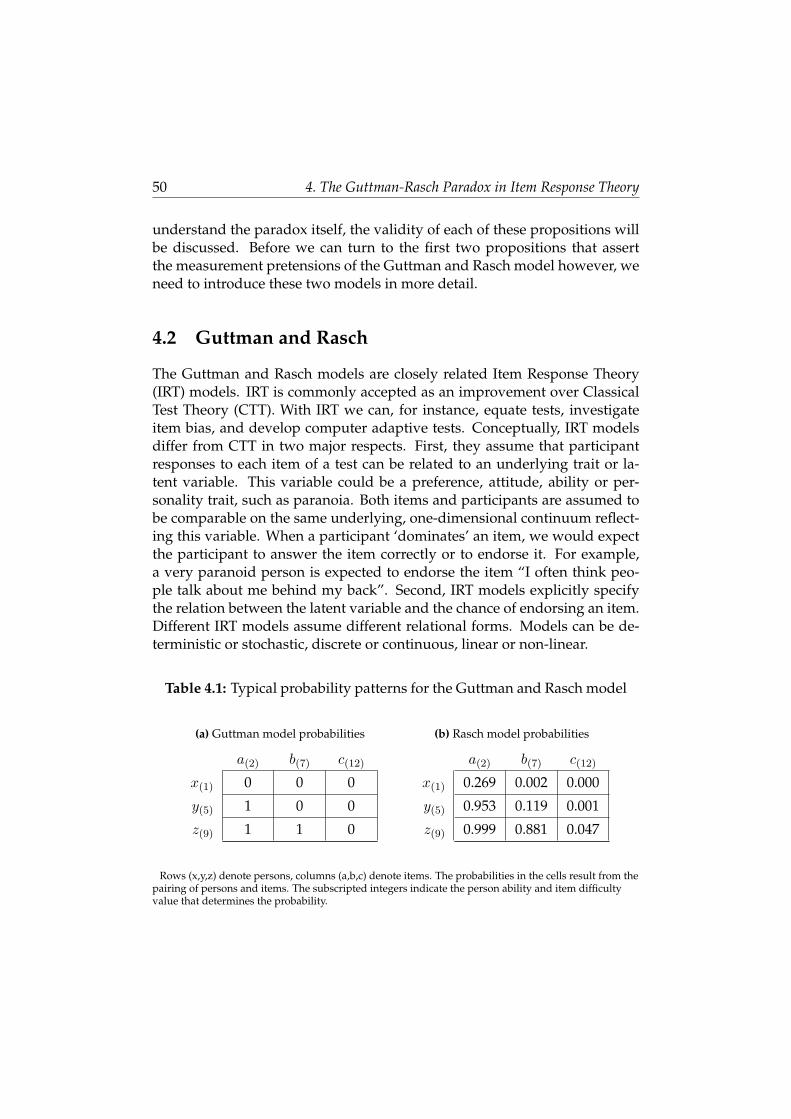
50 4. The Guttman-Rasch Paradox in Item Response Theory
understand the paradox itself, the validity of each of these propositions willbe discussed. Before we can turn to the first two propositions that assertthe measurement pretensions of the Guttman and Rasch model however, weneed to introduce these two models in more detail.
4.2 Guttman and Rasch
The Guttman and Rasch models are closely related Item Response Theory(IRT) models. IRT is commonly accepted as an improvement over ClassicalTest Theory (CTT). With IRT we can, for instance, equate tests, investigateitem bias, and develop computer adaptive tests. Conceptually, IRT modelsdiffer from CTT in two major respects. First, they assume that participantresponses to each item of a test can be related to an underlying trait or la-tent variable. This variable could be a preference, attitude, ability or per-sonality trait, such as paranoia. Both items and participants are assumed tobe comparable on the same underlying, one-dimensional continuum reflect-ing this variable. When a participant ‘dominates’ an item, we would expectthe participant to answer the item correctly or to endorse it. For example,a very paranoid person is expected to endorse the item “I often think peo-ple talk about me behind my back”. Second, IRT models explicitly specifythe relation between the latent variable and the chance of endorsing an item.Different IRT models assume different relational forms. Models can be de-terministic or stochastic, discrete or continuous, linear or non-linear.
Table 4.1: Typical probability patterns for the Guttman and Rasch model
(a) Guttman model probabilities
a(2) b(7) c(12)
x(1) 0 0 0
y(5) 1 0 0
z(9) 1 1 0
(b) Rasch model probabilities
a(2) b(7) c(12)
x(1) 0.269 0.002 0.000
y(5) 0.953 0.119 0.001
z(9) 0.999 0.881 0.047
Rows (x,y,z) denote persons, columns (a,b,c) denote items. The probabilities in the cells result from thepairing of persons and items. The subscripted integers indicate the person ability and item difficultyvalue that determines the probability.

4.2. Guttman and Rasch 51
The most restrictive model is the Guttman model. This model specifiesthat if participants dominate an item, they will always answer this item andall ‘easier’ items correctly. If an item dominates the participant, the partici-pant will always get this item and all more ‘difficult’ items wrong (Guttman,1950). When such data are coded as zeros and ones, and ordered accordingto persons’ ability and item difficulty, the resulting table will show a perfecttriangular pattern of zeros and ones. An example of such a Guttman patternis provided in Table 4.1a.
Guttman was concerned with deviations from a perfect pattern and theability to use the sum score to order persons. He never presented his modelin terms of a latent variable or a probability of answering items correctly.However, others have done so (e.g., Andrich, 1985) and the Guttman modelis now generally regarded as the most basic IRT model. As such, the Guttmanmodel is a deterministic IRT model: the probability of answering an itemcorrectly is 1 for participants who dominate an item, for the others the prob-ability is 0. The relation between probability of answering an item correctlyand person ability is represented by a step function for each item (see Figure4.1a). The location of the step function on the latent ability scale is deter-mined by the difficulty of the item. Harder items are placed further to theright, requiring a higher ability to answer the item correctly. The model canbe formally represented as follows: P (x+) = 1 if θ > β; else P (x+) = 0,where P (x+) denotes probability of answering an item correctly, θ denotesperson ability and β denotes item difficulty.
The Rasch model can be viewed as a stochastic extension of the Guttmanmodel. The Rasch model specifies the relation between the latent variableand the probability of endorsing the item as a logistic function (Rasch, 1960;see Figure 4.1c). The Rasch model is a restrictive model, but it does allowthe chance of item endorsement to increase as the latent trait increases. Thismakes sense to most people: for any given math problem, participants whoare increasingly good at math will have an increasingly higher probabilityof getting the problem right than people who are bad at math. Data that fita Rasch model will result in estimated probabilities like those presented inTable 4.1b. The Rasch model can be represented formally as follows:
P (x+) =e(θ−β)
1 + e(θ−β).
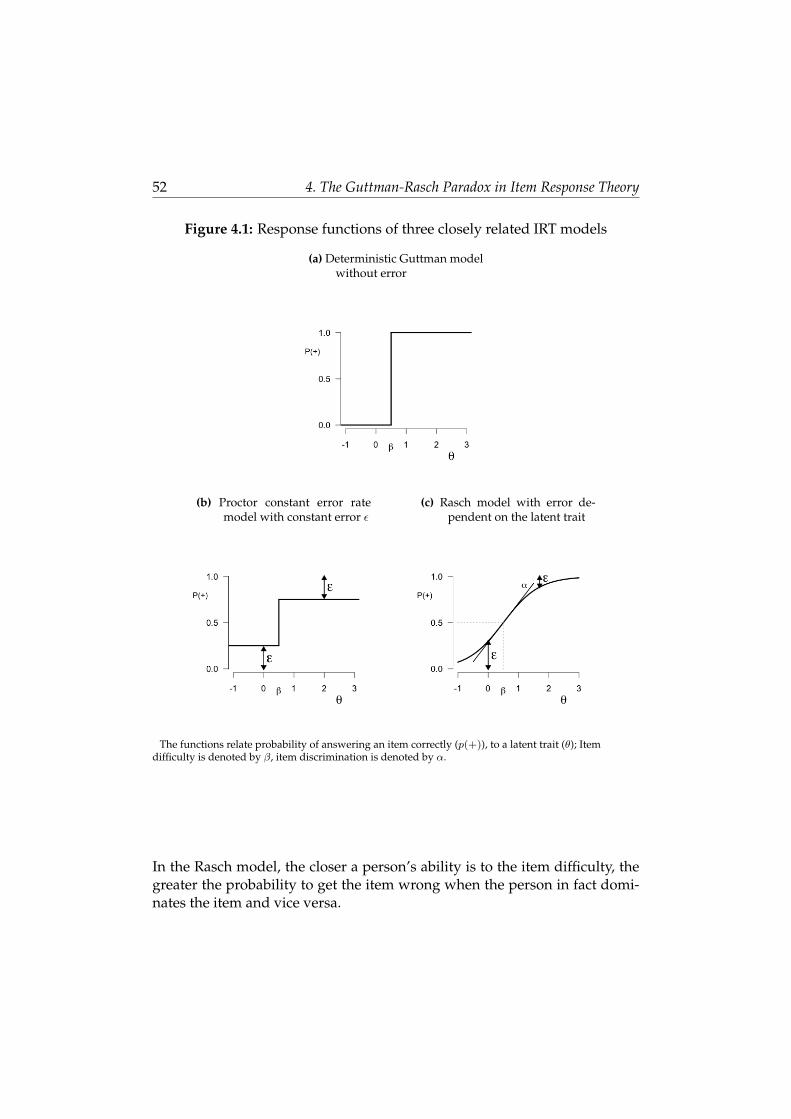
52 4. The Guttman-Rasch Paradox in Item Response Theory
Figure 4.1: Response functions of three closely related IRT models
(a) Deterministic Guttman modelwithout error
(b) Proctor constant error ratemodel with constant error ε
(c) Rasch model with error de-pendent on the latent trait
The functions relate probability of answering an item correctly (p(+)), to a latent trait (θ); Itemdifficulty is denoted by β, item discrimination is denoted by α.
In the Rasch model, the closer a person’s ability is to the item difficulty, thegreater the probability to get the item wrong when the person in fact domi-nates the item and vice versa.

4.3. Measurement Pretensions 53
4.3 Measurement Pretensions
To understand the seemingly paradoxical difference in measurement levelbetween the Guttman and Rasch models it is essential to know why thesemodels are associated with different measurement levels in the first place.The Guttman model only allows ordering of participants and items on thelatent dimension. Differences between participants or items cannot be com-pared meaningfully. It should be noted that although the Guttman paradigmonly allows us to represent the property on an ordinal level, this does notnecessarily mean that the latent property lacks quantitative structure. Adifferent measurement procedure could perhaps be used to represent thesame latent variable on the interval or even ratio level. When we employthe Guttman procedure we simply do not know whether the proposed la-tent variable has quantitative structure. Even if we assume that it does, thereis no way to determine how distances between persons on the selected testitems relate to differences on the latent variable. Perhaps the items were allfairly close together in difficulty, or perhaps the hardest item was dispropor-tionally difficult; we cannot be sure. At best we can say that the sum scoreon the test is related to the latent variable via some monotonically increas-ing function. What the exact shape of this function is cannot be determinedwithout further experimentation or extension of the model.
When item responses fit the Rasch model, this allows us not only to orderparticipants and items, but also to interpret differences between them. Thisis because in the Rasch model differences are considered meaningful. In fact,according to many psychometricians (Rasch, 1960; Brogden, 1977; Perline etal., 1979; Fischer, 1995; Fischer & Molenaar, 1995; Embretson & Reise, 2000;Bond & Fox, 2007) the Rasch model is a probabilistic version of AdditiveConjoint Measurement (ACM), a measurement structure described by repre-sentational measurement theory (Krantz et al., 1971). For different types ofmeasurement structures this formalized theory specifies a set of axioms thatensure measurement at a certain level is possible. According to this theorythe assignment of numerals to objects is considered measurement if the nu-merical relations between the assigned numerals accurately represent (are anisomorphism of) the empirical relations between the objects. The empiricaland numerical relational structure and the axioms that ensure the possibil-ity of representation are specified in a representation theorem. If the axiomshold, we still do not know which subset of the infinite number of possible nu-

54 4. The Guttman-Rasch Paradox in Item Response Theory
merical assignments actually accurately represents the empirical structure.This question is answered in the uniqueness theorem, which specifies whatlevel of measurement is possible by stating the type of transformation thatcan be used to translate all isomorphic (structure-preserving) numerical as-signments into each other (e.g., strictly increasing monotone transformationsdenote ordinal level, linear transformations denote interval level).
In ACM the empirical relational structure is made up of two disjoint setsof objects and their Cartesian product (Luce & Tukey, 1964). In our case thetwo sets of objects are items (I = {a, b, c, . . .}) and persons (P = {x, y, z, . . .}).The Cartesian product is the pairing of each item awith each person x, result-ing in the probability (a, x) that the person will endorse the item. The empiri-cal relation between these objects is a weak ordering on the latent property ofinterest denoted by <. The numerical relational structure that can representthis relation between items, persons and probabilities, consists of the reals,and the numerical relation ≥. The ACM uniqueness theorem specifies thatitems, as well as persons and their pairings (i.e. the item response probabili-ties) can conjointly be represented on the interval level. We can now addressthe truly interesting elements of the representation theorem: the axioms. Forsake of brevity we only give a very general description. A full treatment isprovided in Appendix B.
ACM specifies five axioms, of which the first three are directly empiri-cally testable. The first axiom requires that the ordering of any two proba-bilities is a weak order and is consistent with the ordering between personsor items. If one person has a higher probability of getting an item right thananother person, then the ability of the first person needs to be higher thanthe ability of the second (idem for items and persons reversed). In the Raschmodel the probability is fully determined by the difference between personability and item difficulty. The only way a probability on a given item canbe higher is if the ability of the person is higher. If data fit the mathemati-cal structure of the Rasch model, they will always satisfy this axiom of weakordering. The same goes for the second axiom of independence. This ax-iom requires that the ordering between any two persons remains the same,no matter what item you compare them on (idem for items and persons re-versed). Since the Rasch model produces non-intersecting, monotonicallyincreasing item response curves this axiom cannot be violated. The thirdaxiom, called double cancellation, requires a more complicated form of con-sistency, comparing more than two probabilities at once. This axiom will be

4.4. Why Guttman Fails to Yield Interval Measurement 55
discussed more extensively in the next section. Here it suffices to say thatthe Rasch model meets this axiom for the same reason it meets the first two:its mathematical form simply incorporates it. The same can be said for thelast two axioms. The solvability axiom requires that there is no gap in ourset of items, persons or probabilities. If we know the probability (a, x) ofpersons x answering item a correctly and we have a different person y, thenwe have to be able to find an item b that will give us the same probabilityas (a, x) (idem for items and persons reversed). Because both the probabilityand the latent variable on which the items and persons vary are continuous,this axiom will be met if we imagine we can always find or construct an itemof any difficulty or a person of any ability. A similar argument applies to theArchimedean axiom that requires no difference between persons or items isinfinitely small. This axiom will also be discussed in more detail in the nextsection.
We see that the Rasch model meets the requirements for interval mea-surement. We have also seen that the Guttman model allows for perfectordering of persons and items. What remains somewhat vague howeveris why exactly the Guttman model does not allow for the representation ofquantitative structure. An obvious question therefore presents itself: if theonly difference between the Guttman and Rasch model is the presence oferror, then why does the Guttman model fail to meet the axioms of ACM?One would expect that the removal of error would result in a model with atleast the same measurement level and a higher precision. Examining theanswer to this question will provide more insight into the true nature ofthe paradox. We will therefore evaluate two axioms that prove to be es-pecially problematic for the Guttman model, namely the double cancellationand Archimedean axiom.
4.4 Why Guttman Fails to Yield Interval Measurement
A special case of the double cancellation axiom, the Luce-Tukey condition(Luce & Tukey, 1964; Michell, 1988), will be considered first. The axiom isrepresented graphically in Figure 4.2, where the Cartesian product of items{a, b, c} and persons {x, y, z} is displayed. The Luce-Tukey condition re-quires the resulting probabilities at the tails of the arrows to be comparedwith the probabilities at the arrowheads in Figure 4.2a. If the probabilities
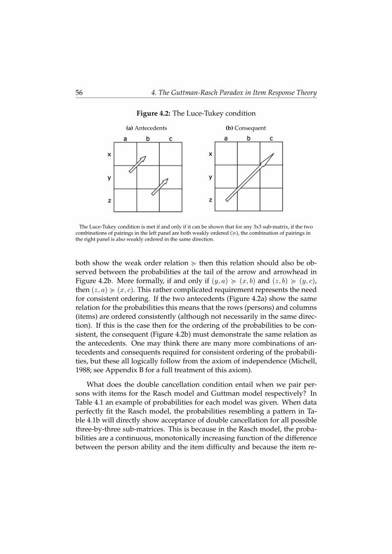
56 4. The Guttman-Rasch Paradox in Item Response Theory
Figure 4.2: The Luce-Tukey condition
(a) Antecedents (b) Consequent
The Luce-Tukey condition is met if and only if it can be shown that for any 3x3 sub-matrix, if the twocombinations of pairings in the left panel are both weakly ordered (<), the combination of pairings inthe right panel is also weakly ordered in the same direction.
both show the weak order relation < then this relation should also be ob-served between the probabilities at the tail of the arrow and arrowhead inFigure 4.2b. More formally, if and only if (y, a) < (x, b) and (z, b) < (y, c),then (z, a) < (x, c). This rather complicated requirement represents the needfor consistent ordering. If the two antecedents (Figure 4.2a) show the samerelation for the probabilities this means that the rows (persons) and columns(items) are ordered consistently (although not necessarily in the same direc-tion). If this is the case then for the ordering of the probabilities to be con-sistent, the consequent (Figure 4.2b) must demonstrate the same relation asthe antecedents. One may think there are many more combinations of an-tecedents and consequents required for consistent ordering of the probabili-ties, but these all logically follow from the axiom of independence (Michell,1988; see Appendix B for a full treatment of this axiom).
What does the double cancellation condition entail when we pair per-sons with items for the Rasch model and Guttman model respectively? InTable 4.1 an example of probabilities for each model was given. When dataperfectly fit the Rasch model, the probabilities resembling a pattern in Ta-ble 4.1b will directly show acceptance of double cancellation for all possiblethree-by-three sub-matrices. This is because in the Rasch model, the proba-bilities are a continuous, monotonically increasing function of the differencebetween the person ability and the item difficulty and because the item re-

4.4. Why Guttman Fails to Yield Interval Measurement 57
Table 4.2: Two problematic Guttman patterns
(a)
a(4) b(6) c(2)
x(5) 1 0 1
y(1) 0 0 0
z(3) 0 0 1
(b)
a(2) b(4) c(5)
x(6) 1 1 1
y(3) 1 0 0
z(1) 0 0 0
Rows (x,y,z) denote persons, columns (a,b,c) denote items. The probabilities in the cells result from thepairing of persons and items. The subscripted integers indicate the ordering of persons and items thatdetermines whether the probability is 1 or 0.
sponse curves are stochastically ordered. This automatically results in themore complicated consistent ordering required by the double cancellationaxiom1. If Guttman probabilities (Table 4.1a) are put to the test however,double cancellation will be violated in many of three-by-three matrices thatare possible.
Two problematic patterns are displayed in Table 4.2. In both cases theantecedents show an equivalence relation (0 ∼ 0 or 1 ∼ 1) which conformsto <. In contrast, the consequent shows a simple order relation (1 ≺ 0) thatcontradicts the weak order found in the antecedents. In the Rasch model,differences between persons and items will always result in differences be-tween the associated probabilities.
In the Guttman model this is not necessarily the case. Two persons differ-ing greatly in their ability still have the same probability of 1 for all the itemsthat the person with the lower ability dominates and the probability of 0 forall the items that dominate the person with the higher ability. The lumpingtogether of persons or items in terms of probabilities leads to the rejection ofdouble cancellation in the Guttman model.
1Not everybody accepts this view. Kyngdon (2008a) argues that probabilities in the Raschmodel can satisfy the order axioms (see Appendix B) but not necessarily the double cancel-lation axiom. If this were the case however, the model would not fit. Of course a perfectlyfitting model will never occur in practice, but we are interested here not in practical limita-tions of the model, but in the structural difference between the Rasch and Guttman model,which is what the Guttman-Rasch paradox is about. The fact is that probabilities in a perfectlyfitting Rasch model will always conform to double cancellation.
58 4. The Guttman-Rasch Paradox in Item Response Theory
The Archimedean axiom requires that no difference between objects ineither set is infinitely small. In other words, it ensures that no item difficultyor person ability is infinitely small or large. This cannot be tested empiricallybut we can examine it by imagining we have an infinite supply of items andpersons. Formally it requires one to order items and persons and denote thisorder by using natural numbers. Now if you pair person xi with item a, andyou then take the next person xi+1, it should take a different (more difficultor easy) item b to get the same result. In the Rasch model, this is clearly thecase. If a person with a certain ability answers an easy item, a person with aslightly higher ability would have to answer a more difficult item to get thesame probability of answering this new item correctly. In the Guttman modelthis is not the case. If a person with a certain ability has a probability of 1 toanswer an easy item correctly, a person with slightly higher ability will haveexactly the same probability of answering the item correctly, an essential fea-ture of the Guttman model. It does not take a different (more difficult) itemto get an equivalence relation between the first person-item pairing and thesecond. The Guttman model therefore also fails the Archimedean axiom.
The reason Guttman fails to conform to ACM is again due to the lump-ing together of different persons or items. The Archimedean axiom mostclearly shows that the objects of measurement need to vary in a continuousmanner. In the case of ACM the objects are not only items and persons butalso probabilities. The discrete nature of the Guttman probabilities precludesmeasurement at the interval level. This can also be understood as follows:the continuous probabilities in the Rasch model that are each associated witha specific ability and difficulty value can only be estimated by using informa-tion from other persons and other items. However, once they are estimatedthe probability of any item contains information on the probabilities on allthe other items. Once we know someone’s probability on one item, we knowthe ability. Combined with knowledge of item difficulties, we know this per-son’s probability on all other items we can imagine, provided they conformto the same model. In the Guttman model this is not the case. Knowing theprobability of 1 or 0 for a certain item does not give information on the prob-ability on all other items. If the probability is 1, we know that this personwill answer all easier items correctly, but we have no idea what this person’sprobability is on more difficult items (and vice versa for probability of 0 andeasier items).

4.5. Rasch Is Guttman Plus Error 59
This is not to say it is impossible that the Guttman model can be associ-ated with interval level measurement. One way this can be conceptualizedis by considering the sum score on the test instead of the response probabil-ities separately. The number of items answered correctly might be able toprovide more than just the ordering of persons and items if we consider adifferent representational structure and add some assumptions concerningrandom selection from an infinite pool of items or persons. However suchan approach is so fundamentally different from the ACM framework whereitems and persons are conjointly measured that we would be comparing ap-ples and oranges. The Guttman model would have to be considered a verydifferent measurement procedure. In that case a difference in measurementlevel would no longer be considered unexpected or paradoxical.
4.5 Rasch Is Guttman Plus Error
We have seen that the essential property responsible for the difference inmeasurement level between the Guttman and Rasch models is the discreteversus the continuous nature of the probabilities incorporated in the respec-tive models. This suggests that error is perhaps not the only or at least not therelevant difference between the models. One could argue however that thetwo are inextricably linked and therefore the distinction is immaterial. Wewill consider whether this argument has merit. To do so we examine in moredetail the proposition that the Rasch model is equivalent to the Guttmanmodel with the addition of error.
In psychometric theory, error is defined as the deviance from the ex-pected response (Lord & Novick, 1968). Concerning the Guttman model wecan be brief. In this model, measurement error is absent. The expected re-sponse is either one or zero, and the deviance from this score is always zero(see Figure 4.1a). This makes the model very hard to fit in practice. For ex-ample, it takes only one very paranoid person who endorses an item indica-tive of low paranoia for the model to fail. To describe such data more accu-rately an obvious approach is to allow for some form of measurement errorin the model. There are at least two different ways to incorporate error in theGuttman model. In the first approach it is assumed that deviations from theexpected response are independent of the ability of the subject. For instance,in the Proctor constant error rate model (Proctor, 1970), the probability of

60 4. The Guttman-Rasch Paradox in Item Response Theory
a deviation from the expected response, ε, is constant. It does not matterwhether the ability is greatly or only slightly above (or below) the item dif-ficulty. The simplest version of this model is represented in Figure 4.1b. Invariants of the Proctor model, ε may depend on the item or on the value ofthe expected score, but it will not depend on the ability, denoted by θ, in acontinuous way.
In the second approach, it is assumed that the probability of a deviationfrom the expected response does depend on the ability level. In these modelsit is essential that the probability of a deviation decreases monotonically as afunction of the difference between ability of the subject and difficulty of theitem. Put more formally: ε = f(|θ − β|) where f(a) > f(b) for all a > b.Another way to state this assumption is that the item response functionshave to be monotonically increasing in θ. The Rasch model, with its itemresponse curve represented in Figure 4.1c, fits into this second category.
We now consider the relation between the Guttman and Rasch modelsin terms of IRT parameters. The Rasch model contains measurement errorthat one would prefer to minimize. In IRT models the relevant parameteris the discriminatory power of an item, which is represented by the slope ofthe item response curve. Items with high discrimination, i.e. steep slopes,differentiate well between persons in a specific range of the latent variable.In the Rasch model the slope of the curve, i.e. the discrimination of an itemis not a parameter but a constant. Items are all required to have the sameslope or discrimination. However, we could imagine changing the wordingof the items or the testing procedure to make all items more discriminating.In this light, reconsider for a moment the curve in Figure 4.1c. For any givenability value, the error becomes smaller when the slope of the curve, denotedby α, becomes steeper. A good test therefore consists of items with highdiscrimination2.
Suppose we apply this adage in the extreme. If we keep improving theitems by removing error and therefore make them even more discriminating,the paradox emerges. The slope of the response curves become so steep thatin the limit our Rasch items turn into Guttman items and we are left with an
2It is of course also important that the items vary in difficulty in the range of interest.High ability participants who are presented with items that strongly discriminate, but onlyon a much lower ability level, will answer all the items correctly, resulting in very low mea-surement precision (in terms of item information, not retest reliability).

4.6. Error that Improves Precision 61
ordinal scale. Thus, by removing error from our items we lose the intervallevel. Stated in reverse: to achieve interval level measurement, all we have todo is add error to the deterministic Guttman model. This comes across as aBaron von Munchhausen adventure. We pulled ourselves out of the swampof measurement problems using error as bootstraps. Stated yet another way:we have observed a planetary system where there previously was none to beobserved, just by fogging up the lens of our telescope!
Our unease with this paradoxical effect of error relies heavily on the as-sertion that error is the only difference between the two models. Mathemat-ically it is true that in the limit we arrive at the Guttman model if we letthe discrimination of the items approach infinity in the Rasch model. In thissense the difference between the two models is indeed error. However, wesaw earlier that the use of discrete versus continuous probabilities is perhapsa more relevant difference between the models. If we consider the differentways error can be added to the Guttman model we see that this discreteversus continuous characteristic is indeed more relevant and not an imma-terial by-product of error per se. One cannot achieve a higher measurementlevel by adding just any error. The Proctor constant error model for instancecan also be considered Guttman plus error. However, there is no famousGuttman-Proctor paradox. This is of course because the error added to pro-duce the Proctor constant error rate model results in discrete probabilities. Itis not error in general that allows for interval level measurement, but a veryspecific characteristic of the special type of error incorporated in the Raschmodel, namely the continuity of probabilities and their systemic dependenceon the latent ability, that allows for the specification of a monotonically in-creasing relation between items and persons.
4.6 Error that Improves Precision
Although we have shown that error in itself is not responsible for the differ-ence in measurement level, it remains counter-intuitive to introduce continu-ity by letting it ride piggy-back on the shoulders of a highly specific type oferror. One would think error, no matter how special, cannot bear informationconcerning the property we measure – it is merely a nuisance that restrictsour measurement precision. This last proposition plays an important role inperpetuating the Guttman-Rasch paradox. However, the proposition is not
62 4. The Guttman-Rasch Paradox in Item Response Theory
only irrelevant, since it focuses on error instead of continuity, it is also false.Even though untutored intuition has it that measurement error should al-ways decrease the quality of our measurements, there are in fact a numberof well-known cases where adding noise to a measurement process is ben-eficial. This phenomenon is generally referred to as stochastic resonance, aterm used to describe the enhancement of a signal by adding noise in certainnonlinear systems. It occurs when a weak signal, often in bistable systems, isamplified by noise. Stochastic resonance was originally proposed to accountfor the periodicity of ice ages, but has since been shown to occur in manydifferent systems (Gammaitoni, Marchesoni, Menichella-Saetta, & Santucci,1989; Wiesenfeld & Moss, 1995).
An example that is particularly interesting in the context of the disap-pearing planets analogy concerns the improved detection of faint stars byadding noise. These stars can be detected better against a slight backgroundfog than against a perfectly black night sky (Dunlop, 1991). Another exampleof stochastic resonance is the enhancement of audio signals perceived withand without hearing aids by adding white noise (Zeng, Fu, & Morse, 2000;Chatterjee & Robert, 2001; Ries, 2007). In a similar vein, the perception ofwater movement in the mechanoreceptor cells of crayfish was enhanced byrandomly perturbing these receptor cells (Douglass, Wilkens, Pantazelou, &Moss, 1993).
A process related to stochastic resonance is dithering. In digital signalprocessing repeated quantization of analog signals may lead to correlatederrors in the resulting signal, leading to large artifacts. By adding dither(noise), to the quantization process, correlated errors are avoided, and bet-ter results are obtained (Schuchman, 1964). Optimization provides anotherexample. In simulated annealing, global solutions are found, and local so-lutions are avoided, by making many non-optimal steps in the initial phaseof the search (Kirkpatrick, Gelatt, & Vecchi, 1983). These examples showthat the relation between measurement error and precision is a complicatedone. Noise can apparently contain information on the latent property, whichmeans there has to be some systematic relation between the error and thelatent variable. To illustrate how such a relationship can be conceptualized,we present a simple example inspired by Lumsden (1976).
Suppose we want to measure the length of a number of people, say A,B, C and D with lengths of 160 cm, 165 cm, 190 cm, and 195 cm. Further-
4.6. Error that Improves Precision 63
more, suppose we – being social scientists, lacking the rigorous measure-ment instruments of physics – have no clue about the actual lengths. Wetherefore resort to a procedure that is familiar to us, the application of pair-wise comparisons. Because we are aware of the high risk of measurementerror we repeat our comparisons several times, just to be sure. If we let ayoung PhD student, of sufficient height and with good eyesight, repeatedlycompare the persons in a precise way, D is always larger than C, B and A,C is always larger B and A, and B is always larger than A. This results inan ordinal Guttman scale. Now we ask a somewhat older, farsighted profes-sor to repeat the procedure. Unfortunately this professor forgot her glassesand makes several mistakes. Obviously, she makes more errors when shecompares A and B and when she compares C and D, because these are closetogether and therefore harder for her to judge. For the same reason, errorsare less probable when she compares B and C. This gives her quantitativeinformation. Because she makes more errors when comparing A and B, andC and D she can infer that the differences between A and B and between Cand D are small relative to the difference between B and C (and A and C andB and D). She can even make a quantitative estimation of these differences,which may be a relatively accurate estimation of the real differences. Herethe paradox reappears: the farsighted professor achieves an improvement inprecision by making mistakes.
A simulation of this example will illustrate the beneficial effect of errormore clearly. Persons A, B, C, and D (respective lengths 160, 165, 190 and195 centimeters) were compared. For each unique comparison a point wasawarded to the longest person, resulting in a number of ‘wins’ for each per-son. To simulate measurement error, normally distributed noise was addedto the actual difference in length for each comparison. The standard devia-tion of the distribution providing the noise varied from 0 to 30. The compar-isons were repeated 1, 2, 5, 10, 20 or 50 times. Each of these ‘trials’ that variedin amount of error and number of repetitions, was simulated 500 times. Tosee whether the added error resulted in a better or worse representation ofthe length of persons A, B, C and D, the root mean square error (RMSE) ofthe number of wins and the actual length (both scaled to z-scores for eas-ier interpretation) was calculated for each trial. Since the actual length andnumber of wins were both scaled to have a mean of zero and a variance ofone, the RMSE will be zero if the number of wins perfectly represents thelength and will increase as the number of wins becomes a less perfect linear

64 4. The Guttman-Rasch Paradox in Item Response Theory
representation of the actual length. Figure 4.3a shows that adding noise re-sults in a clear decrease in the RMSE, which means that precision improves.If we choose a large number of comparisons, we may even allow for highlevels of noise. The optimal level of precision in this simulation is reachedwhen error with a standard deviation between 5 and 10 is added.
Whether the beneficial effect of error appears depends on many things,among which the measurement procedure and the distribution in the sam-ple. If the simulation is performed with the same scoring-procedure but withlengths of 160, 170, 180, and 190 centimeters, adding error does not improvemeasurement precision (i.e., does not decrease the RMSE). The results arepresented in Figure 4.3b. This result is due to the way we set up our mea-surement procedure. If, instead of looking at the number of wins per per-son, we compare each win or loss (scored 0 or 1) per unique comparisonto the difference in actual length, the distribution of lengths becomes irrele-vant. The results of the simulation using this alternative scoring method arepresented in Figures 4.3c and 4.3d for the non-equidistant and equidistantlengths respectively. This time the RMSE decreases (i.e. precision improves)in both the equidistant and the non-equidistant case when error is added,albeit only when we repeat our procedure many times. The positive effect oferror is much more dramatic, especially with many repetitions. The overallprecision of the alternative scoring method is much lower (RMSE is higher)than that of the original method however, because it is much more indirect.Of course indirect methods like paired comparison are often the only onesavailable to represent latent properties in psychological research.
The point of these examples is to show that error, when dependent on thelatent property, can help to increase measurement precision. Whether it doesso in a particular research situation depends on the presence of quantitativestructure in the latent property, on what measurement procedure was used,on the amount of error in the procedure, and in some cases on the spacing ofobjects in the sample. Although the effect of error on precision is probablyonly favorable in very few cases, the main point here is to establish a proofof principle: a positive effect of error on precision is possible. A favorableeffect of error on precision should therefore not necessarily be consideredparadoxical. As a result, our untutored intuition that error should not im-prove precision cannot bolster a general argument against the claim that theRasch model yields interval level measurement. Since the conditions for afavorable effect of error to occur are very restrictive, and since the example

4.6. Error that Improves Precision 65
Figure 4.3: The measurement of length through paired comparison
(a) Non-equidistant, scoring of winsper person
(b) Equidistant, scoring of wins perperson
(c) Non-equidistant, scoring of winsper comparison
(d) Equidistant, scoring of wins percomparison
The precision of measuring length of four persons using paired comparison is ascertained.Non-equidistant refers to a set of persons with actual lengths of 160, 165, 190 and 195 cm; Equidistantrefers to a set of persons with actual lengths of 160, 170, 180 and 190 cm. SD indicates the standarddeviation of the normally distributed error added to comparisons. The lines represent different numberof repeated comparison. A score of one can either be awarded per person or per comparison. The RMSEof the score and the length (difference in case of scoring per comparison) indicates measurementprecision. A lower RMSE value indicates higher precision.
– while informative – does not match typical applications of IRT models wepresent a third simulation that directly involves the Rasch model.
66 4. The Guttman-Rasch Paradox in Item Response Theory
4.7 Error and Precision in the Rasch Model
The setup of the simulation study is simple. Item responses to 16 items weregenerated according to a Rasch model for 500 subjects. Person ability valueswere sampled from a standard normal distribution. The level of discrimina-tion was varied systematically from very low (.1) to very high (50). For eachlevel of discrimination, the simulation was repeated 50 times. Increasing dis-crimination corresponds to the removal of error, making the item more likea deterministic Guttman item. In terms of the previous example, where aforgetful and farsighted professor made comparisons between the length ofpersons, increasing the discrimination parameter would correspond to pro-viding her with a borrowed pair of glasses: the closer the prescription is toher own glasses, the fewer errors she will make.
In the previous simulation it turned out to be important whether the per-sons were spaced equidistantly. This makes sense from the Rasch perspec-tive. It is not just the discrimination that influences precision when pairwisecomparison is used. The spacing of the items is also important; when itemsare highly discriminating but much too easy, precision will be low for per-sons with higher ability and therefore precision for the entire test will suffer.Therefore the spacing of the item difficulties was investigated by generat-ing six item difficulty distributions. The degree to which a distribution ade-quately covered the distribution of abilities was varied first of all by gener-ating a very narrow and a very wide distribution (as compared to the abilitydistribution). Both these distributions were equidistantly spaced and con-sisted of a single group of items centered around the mean ability. Secondlywe were interested to see how precision would be affected if there was agap in the coverage of the ability scale. Therefore we generated distributionsconsisting of two separate groups of equidistantly spaced items. Again, anarrow and a wide distribution were generated. Finally we were interestedto see how precision in the Rasch model would be affected if the items werenot equidistant. To this end we generated non-equidistantly spaced itemsconcentrated at the mean of the ability distribution and non-equidistantlyspaced items concentrated at the tails of the ability distribution. The six re-sulting distributions are displayed in the right panels of Figure 4.4. The cov-erage of the ability scale can be assessed by comparing the item distributionto the curve in each panel, which represents the ability distribution of thesimulated subjects.

4.7. Error and Precision in the Rasch Model 67
Figure 4.4: The effect of error on measurement precision in the Raschmodel
The effect of error on measurement precision, in terms of RMSE is displayed for the Rasch model with16 items, under varying amounts of error and item difficulty spacing. Higher item discriminationindicates lower error. The different item difficulty distributions are shown in the right panels. A lowerRMSE value indicates higher measurement precision.
From the simulated data, the maximum a posteriori (MAP) estimate ofability was computed3. As before, the root mean square error (RMSE) wascalculated, this time of the estimated and original ability values. This indi-cates how well our ability estimates represent the original ability values. Adecrease in RMSE signals an improvement in precision. In Figure 4.4 themean RMSE of the 50 iterations is reported for each value of the discrimina-tion and item difficulty distribution.
3This estimate is relatively easy to compute because the difficulty parameters are knownfrom the simulation setup. That is, we did not need to fit the Rasch model using standardestimation algorithms, which is problematic for data simulated with very high discriminationparameters.

68 4. The Guttman-Rasch Paradox in Item Response Theory
From Figure 4.4 we can derive the following important results. First, inthe normal range of discrimination values (below 5), increasing the discrimi-natory value of items is obviously beneficial to measurement precision, sincethe RMSE decreases. However, in some cases a further increase in discrimi-nation results in an increase in RMSE (case 1: one narrow group; case 3: twonarrow groups; and to a much lesser extent case 5: centered). This meansthat the removal of error until it is almost entirely absent leads to a decreasein measurement precision. Just as in the previous simulation of pairwiselength measurement, precision is optimal when a certain amount of error ispresent, not when error is absent. This allows us to conclude error can alsoenhance measurement precision in this more realistic Rasch set-up. How-ever, this effect only occurs under special circumstances, when the spread initem difficulties is minimal (relative to the distribution of abilities) or con-tains gaps. The beneficial effect of error on precision disappears when itemsare reasonably well spaced over the scale of the latent property.
These simulations have shown that in some cases error can improve pre-cision. In the natural sciences this effect is well-known and sometimes evenactively employed to enhance measurement precision. The proposition thata favorable effect of error on precision is paradoxical therefore cannot forma general, conclusive argument against claims of interval level measurementby the Rasch model. However, in the Rasch simulation we found that thebeneficial effect of error only appears under very select circumstances andthat precision can go both up or down as error increases. This brings atten-tion to another problem with the proposition that error should not improveprecision. This problem concerns the focus on precision.
The assertion that we lose ‘precision’ by removing error from the Raschmodel is unhelpful to say the least. We in fact gain precision in the sensethat we are now able to observe order perfectly, without fault. If we inter-pret ‘precision’ as ‘the proximity between the observed and latent scores’then precision is gained or lost, depending on the circumstances. Only ifwe take ‘precision’ to mean ‘information concerning quantitative structure’,is Michell’s assertion correct. Interpreted as such, we indeed lose precision,but this is not an unfortunate side-effect of our noble effort to minimize error.We have purposefully discarded useful information; a drop in measurementlevel is therefore to be expected and can hardly be considered paradoxical.

4.8. Discussion 69
4.8 Discussion
In our analysis of the Guttman-Rasch paradox, and its use as an argumentagainst the interval level claim by advocates of the Rasch model, we haveshown three things. First, we focused on the measurement pretensions ofboth models in general and the requirements for interval level measurementin particular. We showed that the Guttman model fails these requirementsbecause it employs discrete probabilities where the Rasch model uses con-tinuous probabilities. It is not the removal of error per se, but the transfor-mation of the Rasch probabilities into discrete ones and zeros that preventsus from accessing the quantitative structure that is present in the underlyingvariable. The assertion that the removal of error from the Rasch model ob-viously presents an overly simplified picture of the relation between the twomodels.
Second, to show that our focus on continuity indeed constitutes a mean-ingful distinction relevant to understanding the paradox, we investigated thedifference between the models in terms of error in more detail. The proposi-tion that the Rasch model is equivalent to the Guttman model with the addi-tion of error should also be considered too general a statement. Moving be-tween the Guttman and Rasch model involves more than just the general ad-dition or removal of error. Error can be added to the deterministic Guttmanmodel in many different ways, not all resulting in interval level measure-ment. Only the special type of error incorporated in the Rasch model, charac-terized by its continuous nature and relation to the latent variable, producesthis change in measurement level.
Third, the proposition that error cannot improve precision was shown tobe unfounded. There are indeed cases where error can enhance precision.Using three simulations it was demonstrated how such a beneficial effect oferror can arise. Error can provide more information about the latent prop-erty when the expected number or size of errors is related to the size of in-tervals or values on the latent property. In such cases, removing error cannon-paradoxically have a negative effect on precision. This result was alsofound for the Rasch model, but only when the items are spaced very awk-wardly. When the items cover the entire range of the latent property withno big gaps in between, removing error generally improves precision. Er-ror and precision are sometimes monotonically related and sometimes not,

70 4. The Guttman-Rasch Paradox in Item Response Theory
depending on the circumstances. This has little to do with measurementlevel however. Phrasing the Guttman-Rasch paradox in terms of precisiondeflects our attention from the question that actually requires explanation,namely why removal of error results in a drop in measurement level.
We have already seen that the removal, not of error in general, but ofcontinuity is the decisive factor here. We have also seen that error is not asunlikely a candidate to provide information about the latent property as wemight have thought. By removing the particular type of error that is embed-ded in the Rasch model we are throwing away information about the latentproperty, just as we lose information about the difference in lengths betweenpersons when we provide the nearsighted professor with her glasses. If aperson’s probability of an error is large, then we know that this person’s abil-ity is very close to the item difficulty. By making the probability a discrete0 or 1, we lose this information. A drop in measurement level due to activedismissal of information, although seeming unusual if formulated in termsof precision, is not paradoxical at all. The Guttman-Rasch paradox shouldtherefore be considered a chimera.
If one wishes to contest the claim of interval measurement by the Raschmodel, one needs to present an argument different from the Guttman-Raschparadox. One avenue is to object to the use of probabilities as objects ofmeasurement on the basis that additive conjoint measurement requires theseobjects to be spatio-temporally located (Kyngdon, 2008a, 2008b; Borsboom &Zand Scholten, 2008; Michell, 2008a). This objection does not bear directly onthe Guttman-Rasch paradox, since both models incorporate probabilities andtherefore sin equally against the assumptions of representational measure-ment theory. However we can see that it is quite a leap to view a probabilitythat can never be observed directly as a form of measurement on par withsay, the recording of a person’s length. However if we imagine repeatedlyadministering the test and replacing the probability with a proportion, thisleap becomes less extreme. The proportions can now be observed and therequirements placed upon them empirically tested. This does require eithera substantive assumption or the effort required to experimentally investigatethem. We agree with opponents of the claim of interval level measurementby the Rasch model that such assumptions are made much too easily andexperimental testing is sorely lacking. We do believe however that this is aproblem that is in principle surmountable, it just has not been addressed yet.

4.8. Discussion 71
Another objection is that an ACM framework should apply to generalsets of objects, not a specific subset of items or persons. The introductionof a new, inconsistent object could easily lead to rejection of the axioms(Kyngdon, 2008a; Michell, 2008a). This argument is supported by the factthat it is not always easy to fit a Rasch model to data. One can imagine thatit is tempting to discard items that do negatively affect model fit, even whenthe substantive reasons for considering the item unidimensionally indicativeof the latent property remain unchanged. This goes against the foundationsof ACM, which require the specification of a well-defined, and in most cases,infinite set of objects. We agree that claims of interval level measurement aremade far too easily for tests that consist of conveniently selected items. Thisdoes not mean however that the Rasch model can never be associated withinterval level measurement.
To conclude our discussion of the paradox we return to the disappear-ing planets analogy. In this analogy, the observation of a planetary system,or lack thereof, is compared to the assumption of an interval level, or lackthereof, depending on the presence or absence of error. Similar to the focuson error and precision, this analogy can be considered somewhat mislead-ing. The astronomers suddenly stop observing a physical object when erroris removed from their measurement instrument. Psychometricians do notsuddenly stop observing qualitative relations because error was removed.They are no longer able to detect the quantitative structure present in theserelations because they use a fundamentally different measurement proce-dure. The Rasch procedure requires the psychometrician to assume a latentproperty and a specific functional relation between this property and theprobability of answering an item correctly. The claim of interval measure-ment applies to probabilities, which is still considered controversial by some(Kyngdon, 2008a; Michell, 2008a).
If we make use of the Guttman model we do not have to consider proba-bilities or make strong assumptions. We do have to settle for a discrete mea-surement procedure however, which is intrinsically different from the Raschmodel. We also have to accept that we have to purposefully disregard infor-mation about the latent property that is contained within the measurementerror of the Rasch model. Psychometricians are therefore better compared toastronomers who can all of a sudden no longer observe a planetary system,not because the initial observation was due solely to error, but because theyhad to change from using an infrared telescope to using binoculars. These as-

72 4. The Guttman-Rasch Paradox in Item Response Theory
tronomers would certainly not find the disappearance of the planets suspectper se. And even if they did, it would be highly unlikely that they woulddiscard the infrared telescope, blaming it for seeing the planetary system inthe first place.

Chapter 5
How to Avoid Misinterpretation of InteractionEffects
The only possible interpretation of any researchwhatever in the ‘social sciences’ is: some do, somedon’t.
Ernest Rutherford
Abstract
Inferences about interactions can be invalid due to arbitrary choice of measure-ment scale. Such inferences are at risk when ordinal observations are assumedto represent a quantitative underlying property that is related to the observedvalues via a monotonically increasing function as in Item Response Theory.With a simulation study, the risk of inferential error concerning interaction ef-fects is investigated under conditions that are typical for experimental studiesin psychology. A standard ANOVA F-test shows inferential errors if the trueeffect consists of two main effects, an order-independent, minimal or even apartial interaction in some cases. However, inferential error only occurs whentest difficulty is ill-matched to the latent abilities in the sample and test dis-crimination is high. When true interactions are present, this result is morepronounced when sample size is small. When true interactions are lacking,this result is mitigated by larger sample size. Box-Cox transformed observedscores show much less inferential error. Previous results are combined withcurrent results into a flowchart to provide an easy reference.
74 5. How to Avoid Misinterpretation of Interaction Effects
5.1 Arbitrary Interactions
Experimental psychologists aim to draw general conclusions about psy-chological properties based on their particular research findings. For ex-
ample, a higher mean IQ score for Asians, as compared to Caucasians, mightbe used to conclude that Asians are more intelligent. However, experimentalresearchers have to be very cautious when making an inference about an un-derlying psychological variable (intelligence) based on observed results (IQscores). There are many well-known methodological threats to the validityof such conclusions. One threat that is rarely addressed, even though it canhave a serious effect on the substantive interpretation of research findings,occurs when we employ a statistical test that is inappropriate with respect tothe measurement level of the dependent variable.
A statistical test is inappropriate if it makes use of either ordinal, inter-val or ratio level properties, while the observed data represent the underly-ing variable on a lower measurement level. Such a test can lead to differentconclusions, when performed on transformed scores that still correctly rep-resent the underlying property. Tests of interaction effects, which are verycommon in experimental studies in psychology, are especially vulnerable tothis threat.
We present a comprehensive simulation study, investigating importantfactors that increase the risk of invalid inference concerning interaction ef-fects. We focus on factors that are typical and therefore highly relevant forexperimental research. In doing so, we also provide a general reference forapplied and experimental researchers, allowing easy identification of factorsassociated with higher risk for inferential error. Before we can identify thesefactors, we will start by discussing what makes an inference invalid in thefirst place1.
5.1.1 Legitimate Inference
Consider a factitious study into the effect of alcohol on spatial ability. Sup-pose we compared the number of errors men and women make on a spatialability test. In the experimental condition, the participant is asked to drink
1The next three sections treat the concept of admissible statistics similarly to previouschapters and may therefore be skipped if the reader so wishes.
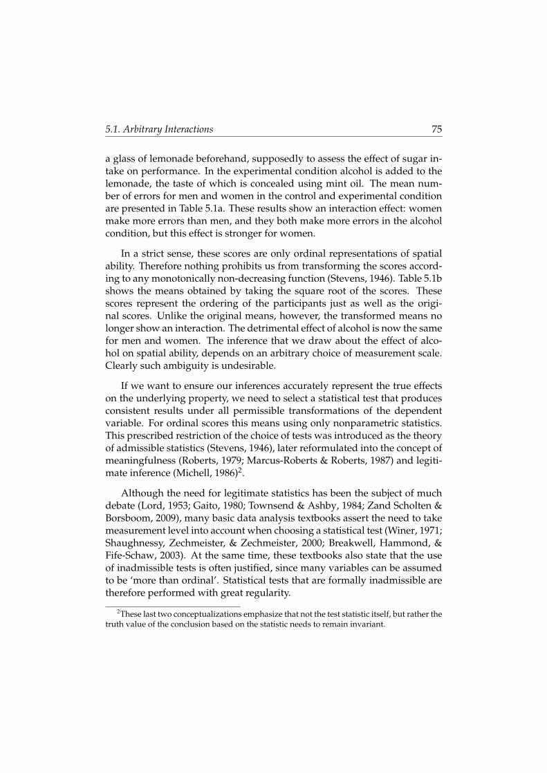
5.1. Arbitrary Interactions 75
a glass of lemonade beforehand, supposedly to assess the effect of sugar in-take on performance. In the experimental condition alcohol is added to thelemonade, the taste of which is concealed using mint oil. The mean num-ber of errors for men and women in the control and experimental conditionare presented in Table 5.1a. These results show an interaction effect: womenmake more errors than men, and they both make more errors in the alcoholcondition, but this effect is stronger for women.
In a strict sense, these scores are only ordinal representations of spatialability. Therefore nothing prohibits us from transforming the scores accord-ing to any monotonically non-decreasing function (Stevens, 1946). Table 5.1bshows the means obtained by taking the square root of the scores. Thesescores represent the ordering of the participants just as well as the origi-nal scores. Unlike the original means, however, the transformed means nolonger show an interaction. The detrimental effect of alcohol is now the samefor men and women. The inference that we draw about the effect of alco-hol on spatial ability, depends on an arbitrary choice of measurement scale.Clearly such ambiguity is undesirable.
If we want to ensure our inferences accurately represent the true effectson the underlying property, we need to select a statistical test that producesconsistent results under all permissible transformations of the dependentvariable. For ordinal scores this means using only nonparametric statistics.This prescribed restriction of the choice of tests was introduced as the theoryof admissible statistics (Stevens, 1946), later reformulated into the concept ofmeaningfulness (Roberts, 1979; Marcus-Roberts & Roberts, 1987) and legiti-mate inference (Michell, 1986)2.
Although the need for legitimate statistics has been the subject of muchdebate (Lord, 1953; Gaito, 1980; Townsend & Ashby, 1984; Zand Scholten &Borsboom, 2009), many basic data analysis textbooks assert the need to takemeasurement level into account when choosing a statistical test (Winer, 1971;Shaughnessy, Zechmeister, & Zechmeister, 2000; Breakwell, Hammond, &Fife-Schaw, 2003). At the same time, these textbooks also state that the useof inadmissible tests is often justified, since many variables can be assumedto be ‘more than ordinal’. Statistical tests that are formally inadmissible aretherefore performed with great regularity.
2These last two conceptualizations emphasize that not the test statistic itself, but rather thetruth value of the conclusion based on the statistic needs to remain invariant.
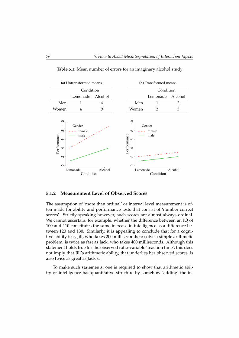
76 5. How to Avoid Misinterpretation of Interaction Effects
Table 5.1: Mean number of errors for an imaginary alcohol study
(a) Untransformed means
Condition
Lemonade Alcohol
Men 1 4
Women 4 9
(b) Transformed means
Condition
Lemonade Alcohol
Men 1 2
Women 2 3
Gender
female
male
Lemonade Alcohol
02
46
810
Perf
orm
ance
Condition
Gender
female
male
Lemonade Alcohol
02
46
810
Perf
orm
ance
Condition
5.1.2 Measurement Level of Observed Scores
The assumption of ‘more than ordinal’ or interval level measurement is of-ten made for ability and performance tests that consist of ‘number correctscores’. Strictly speaking however, such scores are almost always ordinal.We cannot ascertain, for example, whether the difference between an IQ of100 and 110 constitutes the same increase in intelligence as a difference be-tween 120 and 130. Similarly, it is appealing to conclude that for a cogni-tive ability test, Jill, who takes 200 milliseconds to solve a simple arithmeticproblem, is twice as fast as Jack, who takes 400 milliseconds. Although thisstatement holds true for the observed ratio-variable ‘reaction time’, this doesnot imply that Jill’s arithmetic ability, that underlies her observed scores, isalso twice as great as Jack’s.
To make such statements, one is required to show that arithmetic abil-ity or intelligence has quantitative structure by somehow ‘adding’ the in-

5.1. Arbitrary Interactions 77
telligence of any two people and showing that their combined intelligencecan be compared consistently to the combined intelligence of any other twopeople (Krantz et al., 1971). Of course the concatenation does not have tobe direct, or even additive. Few psychological properties lend themselvesto direct or indirect forms of concatenation however, which leaves us withat most an ordinal level of measurement in many situations3. Without fur-ther qualification this means almost all inferences in experimental psychol-ogy based on parametric tests, including inferences about interactions basedon ANOVA, would have to be considered questionable. Fortunately this con-clusion is premature.
5.1.3 Linearity and Inadmissible Tests
For many questionnaires and tests, the advice to treat ordinal scores as in-terval level scores, and to perform strictly inadmissible tests, is sound. If therelation between the ordinal observed scores and the underlying latent inter-val variable is linear, the observed scores will produce differences in groupmeans that closely represent the true effects on the latent property (all elsebeing equal)4. It is generally assumed that tests of sufficient length, consist-ing of Likert-scale items with around five to seven response categories willresult in a near-to linear relation between latent and observed scores (Dolan,1994). For a specific subset of tests however, it is not feasible to assume alinear relation between observed scores and the latent property. In IRT it isassumed that for dichotomous items, the relation between the latent vari-able and the probability of answering an item correctly is best described by alogistic-type function. For the total test score this leads to a nonlinear relationbetween the observed and latent level.
3A noted exception to this rule, at least according to some (Embretson & Reise, 2000; Bond& Fox, 2007), is provided by the Rasch model. This Item Response Theory (IRT) model canbe viewed as a form of additive conjoint measurement. This involves the concatenation ofitems and persons resulting in pairings that correspond to the probability for a person to getthe item right. If these pairings can be shown to adhere to a set of axioms (Luce & Tukey,1964) then interval measurement is said to be achieved. (See Kyngdon, 2008a, Borsboom &Zand Scholten, 2008 and Michell, 2008a, for a discussion concerning this claim.)
4It is important to note that the assumption of a linear relation between latent and ob-served scores presupposes that the underlying property has quantitative structure. This as-sumption is almost never plausibly supported, empirically or otherwise. See Michell for adetailed discussion on this topic (Michell, 1997).
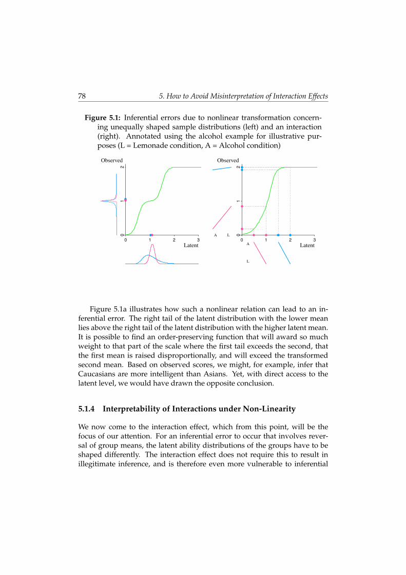
78 5. How to Avoid Misinterpretation of Interaction Effects
Figure 5.1: Inferential errors due to nonlinear transformation concern-ing unequally shaped sample distributions (left) and an interaction(right). Annotated using the alcohol example for illustrative pur-poses (L = Lemonade condition, A = Alcohol condition)
0 1 2 3
01
2
Latent
Observed
ll
ll
0 1 2 30
12
Latent
Observed
l
l
l
l
l l l lA L
A
L
Figure 5.1a illustrates how such a nonlinear relation can lead to an in-ferential error. The right tail of the latent distribution with the lower meanlies above the right tail of the latent distribution with the higher latent mean.It is possible to find an order-preserving function that will award so muchweight to that part of the scale where the first tail exceeds the second, thatthe first mean is raised disproportionally, and will exceed the transformedsecond mean. Based on observed scores, we might, for example, infer thatCaucasians are more intelligent than Asians. Yet, with direct access to thelatent level, we would have drawn the opposite conclusion.
5.1.4 Interpretability of Interactions under Non-Linearity
We now come to the interaction effect, which from this point, will be thefocus of our attention. For an inferential error to occur that involves rever-sal of group means, the latent ability distributions of the groups have to beshaped differently. The interaction effect does not require this to result inillegitimate inference, and is therefore even more vulnerable to inferential

5.1. Arbitrary Interactions 79
errors. Figure 5.1b illustrates how an interaction effect can be susceptible toinferential error. Two main effects on the latent variable (parallel lines) aretransformed by a logistic function that stretches the lower end of the scale,thereby disproportionally lowering the bottom mean and creating an inter-action (non-parallel lines).
If it is plausible to assume that the observed scores are linearly relatedto the underlying variable, we have little reason for concern. But what ifwe assume a nonlinear relation? Does this mean all interactions should thenbe considered uninterpretable? Fortunately, such a drastic conclusion is notnecessary. Interactions come in many shapes and sizes, not all of which areequally vulnerable to invalid inference. Assuming all four group means dif-fer, the means can be ordered in 24 different ways. These 24 permutationscan be categorized into three classes of effects: crossing interactions, partialinteractions and order-independent (main or interaction) effects. When cer-tain group means are equal, additional types of main effects and interactionsoccur (see Appendix C).
Figure 5.2 displays these effects, annotated in line with the alcohol exam-ple to facilitate interpretation. The crossing interaction entails a reversal ofthe group means between levels of one factor on the other factor (i.e., whensex is plotted on the x-axis the lines still cross). The partial interaction isso named because the group means only reverse for one factor (i.e., whensex is plotted on the x-axis the lines will diverge up and down). The orderindependent interaction and double main effect are both characterized bythe irrelevance of the ordering of the non-extreme means (men in the alco-hol condition and women in the lemonade condition). These means can bereversed without affecting the substantial interpretation of the effect. Theminimal interaction is named for the minimal requirement needed to createit, namely the deviation of only one group mean.
If nothing is known about the form of the functional relation betweenlatent and observed scores, except that it is nonlinear and nondecreasing,then crossing, partial and minimal interactions will always remain consis-tent (Loftus, 1978). For these types of interactions, the effect is entirely de-termined by the ordering of the group means. Uneven stretching of the scalewill affect the size of the group differences, but not the substantive interpre-tation of the effect. The absence of an interaction in combination with exactlyone main effect is also unambiguous, as is the total absence of any effect (i.e.,
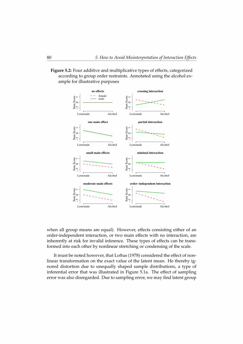
80 5. How to Avoid Misinterpretation of Interaction Effects
Figure 5.2: Four additive and multiplicative types of effects, categorizedaccording to group order restraints. Annotated using the alcohol ex-ample for illustrative purposes
no effects
Lemonade Alcohol
−1
01
Sum
Score
female
male
one main effect
Lemonade Alcohol
−1
01
Sum
Score
small main effects
Lemonade Alcohol
−1
01
Sum
Score
moderate main effects
Lemonade Alcohol
−1
01
Sum
Score
crossing interaction
Lemonade Alcohol
−1
01
Sum
Score
partial interaction
Lemonade Alcohol
−1
01
Sum
Score
minimal interaction
Lemonade Alcohol
−1
01
Sum
Score
order−independent interaction
Lemonade Alcohol
−1
01
Sum
Score
when all group means are equal). However, effects consisting either of anorder-independent interaction, or two main effects with no interaction, areinherently at risk for invalid inference. These types of effects can be trans-formed into each other by nonlinear stretching or condensing of the scale.
It must be noted however, that Loftus (1978) considered the effect of non-linear transformation on the exact value of the latent mean. He thereby ig-nored distortion due to unequally shaped sample distributions, a type ofinferential error that was illustrated in Figure 5.1a. The effect of samplingerror was also disregarded. Due to sampling error, we may find latent group
5.1. Arbitrary Interactions 81
means that differ from the latent means in the population. This can becomea problem when hypothesized effects consist of two or more equal popula-tion means. Two values that are equal will remain equal after any one-to-onetransformation. However, small differences between group means due tosampling error can be exacerbated by nonlinear transformation, thereby re-sulting in large differences in observed group means. To our knowledge thisproblem has not been addressed in the literature so far.
In contrast, the detrimental effect of unequally shaped sample distri-butions has received much more attention. In the simple two-group com-parison or one-way ANOVA case, inference is disambiguated if the groupsare normally distributed with homogeneous variances (Davison & Sharma,1988). Such a restriction preempts the type of invalid inference in Figure 5.1a.However, this approach does not work in factorial ANOVA designs withtwo or more factors (Davison & Sharma, 1990). Combining the results fromLoftus (1978) and Davison and Sharma (1990), we see that the assumptions ofnormality and homogeneity unfortunately fail to provide a way to excludeinferential error concerning order-independent main or interaction effects.Also, the extent of the detrimental effect of sampling error on effects thatincorporate equal means, remains unclear.
5.1.5 Interactions under Specific Non-Linear Assumptions
Besides type of interaction and distributional shape, another factor to con-sider is the exact form of the relation between the latent and observed vari-ables. When this relation is specified, it is possible to investigate the effect ofother research designs and test characteristics on the validity of inferences.Embretson (1996) and Kang and Waller (2005) simulated latent and observedscores using the Rasch model and a two-parameter IRT model, respectively.The impact of main and interaction effect size, item difficulty, item discrimi-nation and test length on the detection of interaction effects was investigated.Inferential errors were found only when the test was too easy or difficult forthe simulated sample of persons. This result was more pronounced whentest length and effect sizes were greater and the test consisted of highly dis-criminating items, i.e., items that differentiate well between values of thelatent ability.

82 5. How to Avoid Misinterpretation of Interaction Effects
These results make sense when we consider the functional form of therelation between scores on, for example, an inappropriately difficult test andthe latent variable. Over the range of the group means, the function willincrease slowly for the lowest means, but faster for the higher means (seeFigure 5.3 for examples). The means are located where the function is ‘leastlinear’ and therefore unequal stretching or condensing of the means is likely,with a higher risk of distorting effects. The longer a test, the more consistentthe item responses will be, resulting in an even stronger floor or ceiling ef-fect. The higher the item discrimination, the steeper the slope of the curve,resulting in more sudden and extreme differential stretching and condensingof the scale. The IRT perspective thus allows us to identify when and whythe relationship between the latent and observed level is more nonlinear andtherefore at risk of producing invalid inferences.
In addition to identifying parameters associated with inferential error,IRT can also help us to avoid inferential error altogether, at least according toEmbretson (1996) and Kang and Waller (2005). They advocate the use of IRTmodeling to obtain latent ability estimates. These estimates can be analyzedin place of the observed sum scores. Although such advice seems sound intheir setting (moderated multiple regression with large sample size), this av-enue is often closed to experimental researchers. In many cases the samplesize in experimental studies is too small to fit an IRT model. Even if esti-mates can be obtained, the model still has to show adequate fit. Obviously,latent ability estimates are not going to provide a one-stop, fix-all solutionto our inferential problems. More insight is needed into the risk of infer-ential error under circumstances that are typical for experimental studies.Also, a method to mitigate inferential error when these risk factors cannot beavoided would form a welcome addition to our statistical toolkit.
5.1.6 Identifying and Avoiding Inferential Errors
By considering a specific non-linear relation, we have further reduced the setof inferentially ambiguous interactions: order-independent effects, and pos-sibly minimal interactions (due to sampling error) are at risk for inferentialerror, but only when the test is mismatched to the abilities of the persons inthe sample. Of course this reduction comes at a cost. We have introducedseveral assumptions in the process, namely that a latent variable exists, thatit has quantitative structure and that this structure is represented by the ob-
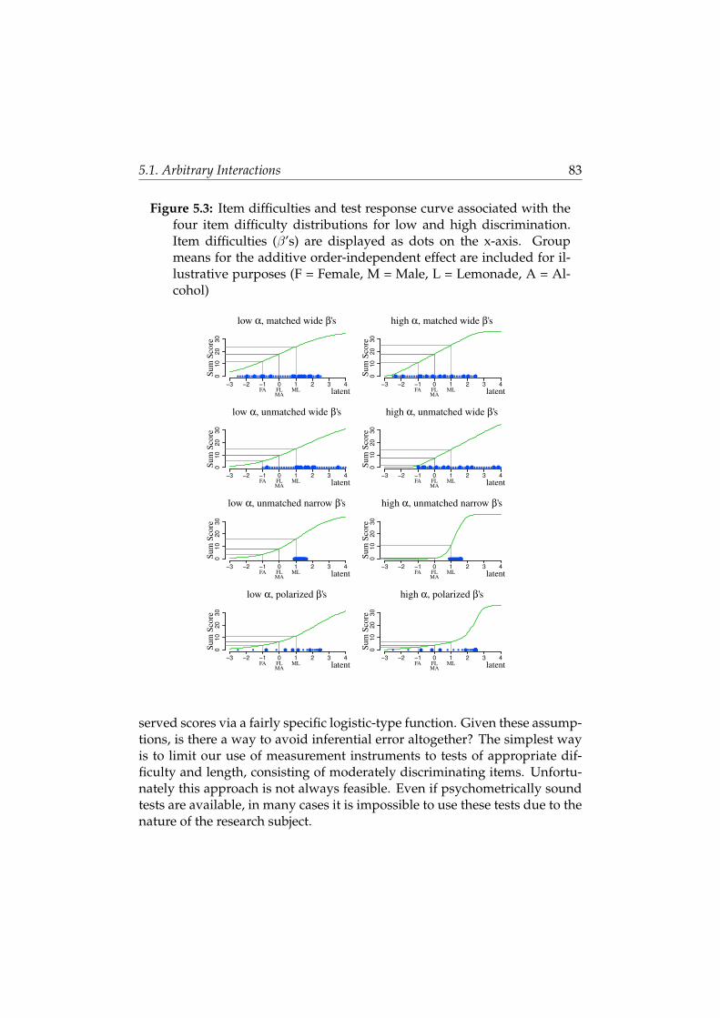
5.1. Arbitrary Interactions 83
Figure 5.3: Item difficulties and test response curve associated with thefour item difficulty distributions for low and high discrimination.Item difficulties (β’s) are displayed as dots on the x-axis. Groupmeans for the additive order-independent effect are included for il-lustrative purposes (F = Female, M = Male, L = Lemonade, A = Al-cohol)
low α, matched wide β's
−3 −2 −1 0 1 2 3 4
010
20
30
latent
Su
m S
core
FLFA MLMA
l l l l l l l l l l l l l l l l l l l l l l l l l l l l l l l l l l l l
low α, unmatched wide β's
−3 −2 −1 0 1 2 3 4
010
20
30
latent
Su
m S
core
FLFA MLMA
l l l l l l l l l l l l l l l l l l l l l l l l l l l l l l l l l l l l
low α, unmatched narrow β's
−3 −2 −1 0 1 2 3 4
010
20
30
latent
Su
m S
core
FLFA MLMA
llllllllllllllllllllllllllllllllllll
low α, polarized β's
−3 −2 −1 0 1 2 3 4
010
20
30
latent
Su
m S
core
FLFA MLMA
llllllllllllllllllllllllllllllllllll
high α, matched wide β's
−3 −2 −1 0 1 2 3 4
010
20
30
latent
Su
m S
core
FLFA MLMA
l l l l l l l l l l l l l l l l l l l l l l l l l l l l l l l l l l l l
high α, unmatched wide β's
−3 −2 −1 0 1 2 3 4
010
20
30
latent
Su
m S
core
FLFA MLMA
l l l l l l l l l l l l l l l l l l l l l l l l l l l l l l l l l l l l
high α, unmatched narrow β's
−3 −2 −1 0 1 2 3 4
010
20
30
latent
Su
m S
core
FLFA MLMA
llllllllllllllllllllllllllllllllllll
high α, polarized β's
−3 −2 −1 0 1 2 3 4
010
20
30
latent
Su
m S
core
FLFA MLMA
llllllllllllllllllllllllllllllllllll
served scores via a fairly specific logistic-type function. Given these assump-tions, is there a way to avoid inferential error altogether? The simplest wayis to limit our use of measurement instruments to tests of appropriate dif-ficulty and length, consisting of moderately discriminating items. Unfortu-nately this approach is not always feasible. Even if psychometrically soundtests are available, in many cases it is impossible to use these tests due to thenature of the research subject.
84 5. How to Avoid Misinterpretation of Interaction Effects
For example, tests used to diagnose psychopathological disorders likedepression or schizophrenia need to discriminate well at the high end of thescale to identify people at risk for suicide or sudden aggressive behavior.Such tests will be inappropriately ‘difficult’ for most of the sample. Anotherexample of a test that is inappropriate by design, occurs when a teachingmethod is so effective that it renders the test too easy for the participantsin the experimental condition while remaining appropriate for those in thecontrol condition. The use of inappropriately difficult tests can also be un-avoidable for more substantive reasons, as in the context of stereotype threat,for example. Stereotype threat occurs when the performance of a stereotypedgroup is lowered compared to the performance of a non-stereotyped group,due to activation of the stereotype (Steele & Aronson, 1995). The detrimentaleffect of the threatening stereotype on performance of the stereotypes grouponly occurs when the possibility of confirming the stereotype is real. For thispossibility to be perceived, the test has to be sufficiently difficult (O’Brien &Crandall, 2003).
Given that mismatched tests cannot always be avoided, and IRT model-ing is rarely a viable option in experimental settings, alternative methodsare needed to signal and possibly mitigate an elevated risk of inferentialerror. With the focus on latent ability estimates, the previous IRT studies(Embretson, 1996; Kang & Waller, 2005) put less emphasis on results pertain-ing to the distributional properties of the observed scores. Inferential errorwas found when the test was mismatched and highly discriminating, whichentails that the lowest scoring groups on a difficult test (highest for an easytest) will show a floor (ceiling) effect. The scores in these extreme groups willbe more heavily skewed and will show less variability. Group differences indescriptive statistics could signal high-risk situations. With standard testsof normality and homogeneity of variances already in place, the requiredadditional effort is minimal.
We therefore conducted a simulation of a typical two-by-two factorial de-sign study. The first aim was to confirm that mismatched item difficulty andhigh item discrimination would result in inferential errors in a typical small-sample, fixed-effects study. The second aim was to assess the impact of sam-pling error. Therefore, all effects presented in Figure 5.2, including the min-imal interaction, were considered. Third, inferential error was assessed fordifferent sample sizes. Since sample size relates directly to statistical powerand generalizability, an effect on inferential error is to be expected. Apart

5.1. Arbitrary Interactions 85
from identifying general factors associated with inferential error, a normal-izing transformation was performed in the hope of suppressing inferentialerror.
5.1.7 Simulation Study
The aim was to investigate the risk of inferential errors for different types ofinteraction effects under conditions typical for experimental studies. A two-by-two fixed effects design was chosen. The effects generated on the latentvariable are the crossing, partial, minimal and order-independent interactionand corresponding main effects depicted in Figure 5.2. Latent ability valueswere transformed into observed scores using the two-parameter IRT model.A test of moderate length was simulated. Sample size, item difficulty anddiscrimination were varied systematically.
To investigate whether increasing sample size would decrease the riskof inferential error, we compared a typically small sample size with a largersample size. Test difficulty was manipulated to produce items that variedin how well they matched latent abilities and to what extent they coveredthe range of abilities. Discrimination was manipulated to be high or low. Tosee how changes in sample size, difficulty and discrimination affect inferen-tial validity, data were simulated repeatedly for each combination of factors.ANOVAs were performed on the latent scores and the observed scores. Thenumber of significant interactions on the latent and observed level were com-pared. Also, several descriptive statistics and a normalizing transformationof the observed scores were considered. Deviations from normality signaledby descriptive statistics and tests could indicate that the risk of inferentialerror is elevated. A normalizing transformation could help to counter thedistortion caused by the nonlinear transformation from latent to observedscores. The exact simulation setup is discussed in more detail below.
86 5. How to Avoid Misinterpretation of Interaction Effects
5.2 Method
5.2.1 Generating latent and observed scores
We simulated an experimental study with two independent factors F1 andF2, each with two levels, and one dependent response variable. The sim-ulation consisted of two steps. First, latent ability values were generatedaccording to the model θ = t + w1 · F1 + w2 · F2 + w12 · F1 · F2, where twas randomly sampled from a standard normal distribution. Factors F1 andF2 indicate assignment to one of two levels (contrast coded -1 or 1) on eachfactor, and w1, w2 and w12 indicate the weights used to determine main andinteraction effects on the latent level. Sample size was set at 120 or 360, re-sulting in group sizes of 30 or 90 respectively. The first choice reflects samplesizes that are generally found in experimental research.
Second, latent scores were transformed into sum scores. Item responseswere generated according to the two parameter logistic model:
pij(+) =exp(α(θj − βi))
1 + exp(α(θj − βi))
Where pij(+) indicates the probability of answering item i correctly for per-son j. θj denotes the latent ability of person j, simulated in step one. βidenotes the item difficulty and α the item discrimination of item i. Althoughitem discrimination was the same for all items in a particular simulated test,discrimination was treated as a factor in the simulation study and was set toeither a high or low value. The probability pij(+) was then recoded into a bi-nary score of 0 or 1, by drawing from a Bernoulli distribution with probabil-ity pij(+). Finally the item responses were added for each person, resultingin sum scores.
5.2.2 Spurious and overlooked interactions
Latent abilities were simulated under either an additive model or a multi-plicative model. In the additive model the interaction term was taken out ofthe model by setting the weight w12 to zero. Except for sampling error, latentabilities will display no interaction under this model. We therefore expectedto find very few significant interactions on the corresponding simulated sum
5.2. Method 87
scores (low Type I error rate). Any significant interaction will therefore bedesignated a spurious interaction. Under the multiplicative model, latentabilities were generated with a non-zero weight w12. Barring sampling error,latent abilities generated under this model will show interactions and there-fore we expected a high number of significant interactions on the simulatedsum scores (low Type II error rate, high power). A non-significant interac-tion effect found under the multiplicative model will be termed an overlookedinteraction.
5.2.3 Types of simulated latent effects
The effects displayed in Figure 5.2 were simulated by choosing differentcombinations of weights w1, w2 and w12. The weights (0.0, 0.0, 0.5) resultsin no main effects under the additive model and a fully crossing interactionunder the multiplicative model. The weights (0.0,−0.5, 0.3) result in onemoderate main effect, and a partial interaction under the additive and multi-plicative model, respectively. The weights (0.3,−0.3, 0.3) result in two smallmain effects under the additive model, and in a minimal interaction underthe multiplicative model. Finally we included the weights (0.5,−0.5, 0.3),that result in two moderate main effects under the additive model, and anorder-independent interaction under the multiplicative model.
5.2.4 Test characteristics
The test consisted of 36 items to simulate a test of moderate length, therebyapproximating the short to moderate test length typically used in experimen-tal studies. Item response probabilities were generated using four differentlygrouped sets of item difficulties. In the first three cases, the item difficul-ties were all equally spaced, either between -2.5 and 2.5 (‘matched wide’),between -1 and 4 (‘mismatched wide’), or between 0.875 and 1.625 (‘mis-matched narrow’). Finally, the spacing between the item difficulties was var-ied by polarizing at the extreme of 2.5 and moving in increasing steps, usinga power function, towards the extreme of -2.5 (‘polarized’). This item dis-tribution was included to simulate tests that are heavily targeted at extremevalues at one end of scale, but that do include a few items that cover the restof the scale to allow for some response variation.

88 5. How to Avoid Misinterpretation of Interaction Effects
Item discrimination was either low (α = 1) or high (α = 4). Figure 5.3 dis-plays the test response curve that relates the latent ability to the sum scoresand the item difficulty values for the four different sets of difficulties andlow and high discrimination. Higher item discrimination corresponds to asteeper test response curve and concentration of item difficulties result inmore changes in slope. These changes in slope will be smoothed by lowdiscrimination, resulting in a more linear curve.
5.2.5 Descriptive statistics and tests
Altogether this study consisted of 128 levels: 2 (additive / multiplicativemodel) × 4 (choice of weights resulting in main / interaction effects) × 4(item difficulty sets) × 2 (item discrimination) × 2 (sample size). For eachcombination of levels the simulation was repeated a 1000 times. For eachof these simulation runs, an ANOVA was performed on the latent and ‘ob-served’ scores, employing a significance level of 0.05. Pearson χ2-tests wereperformed to see if the number of spurious and overlooked interactions ex-ceeded the number of significant results expected due to chance. These testsare not to be confused with the standard χ2-test of independence. Using theBonferroni correction, a significance level of 0.001 was adopted, due to thelarge number of iterations and the considerable number of statistical tests.
Shapiro-Wilks’ test of normality and Levene’s test of homogeneity ofvariances were performed on the observed and latent scores. Skewness andkurtosis coefficients were also considered. We expected non-normality andheterogeneity of variances, especially in the groups with the lowest means.For these groups the latent scores will be transformed according to the leastlinear part of the function that relates the latent and observed level resultingin unequal stretching of the scale and a change in sample distribution. Insuch cases a normalizing transformation could provide a good way to ap-proximate the latent scores without modeling. A byproduct of an attemptto restore the sample distribution to its (assumed) original shape is that un-equally stretched parts of the scale are in effect condensed again. Sum scoreswere therefore transformed according to a Box-Cox transformation. All de-scriptive statistics and analyses that were performed using the original scoreswere also performed using the Box-Cox transformed scores.
5.3. Results 89
5.3 Results
5.3.1 Main Effects Generated by the Additive Model
The primary results of the simulation, generated under the additive model,are presented in Table 5.2. Results generated using small and large samplesizes (N=120, 360) are presented in the same table. The number of significantinteractions, obtained from a standard ANOVA performed on the simulatedobserved scores, is cross-tabulated for all combinations of item difficultiesand item discriminations. Under the additive model, a significant interaction(i.e., a Type I error) is expected in 50 out of a 1000 iterations. The Pearson χ2-test statistics5 and p-values are also provided in Table 5.2. As witnessed bythe non-significant χ2 tests, the number of significant interactions did notdiffer from the expected count of 50 when no main effects or only one maineffect were present. The most extreme deviation constitutes an increase inType I error of less than 1%. Even when discrimination is high and when theitem difficulties are ill-matched to the sample, the conclusion concerning thegroup means is unaffected by the nonlinear relation with the latent ability.
The situation is different when there are two main effects. Only when thetest matches the sample and item difficulties cover the entire ability range,does Type I error rate stay in check. For all three inappropriately targetedtests, increased discrimination leads to more Type I errors. As the test be-comes more inappropriate, Type I error rate goes up, in some cases quitedrastically. For the least appropriate test (unmatched narrow), Type I er-ror rate increases to 44%, and even to 90% for small and large sample sizerespectively, when effect sizes are moderate and discrimination is high. Thepolarized test, which covers the entire range of abilities, albeit very unevenly,shows less dramatic but similarly inflated Type I error rates. Inferential errorclearly forms a substantial problem when the true effect consists of two maineffects, the test is ill-matched to the sample and items are high in discrimi-nation. Increased sample size only aggravates the situation. The χ2-test issignificant in all these cases.
5The χ2 was calculated using both the number of significant and non-significant interac-tions (1000 - #(significant interactions)). Due to limited space, only the number of significantinteractions is displayed.

90 5. How to Avoid Misinterpretation of Interaction Effects
Table 5.2: Number of significant interaction effects (Type I errors) underthe additive model with N=120, 360; The expected count is 50
no effects
N = 120 discrimination
difficulties low high
matched wide 46 55
unmatched wide 55 50
unmatched narrow 59 57
polarized 43 52
χ2(7) 5.24
p-value 0.630
1 main effect
discrimination
low high
45 56
48 45
50 53
56 36
6.97
0.432
2 small effects
discrimination
low high
53 45
43 45
59 110
68 68
93.41
< 0.0001
2 mod. effects
discrimination
low high
43 55
72 78
120 443
96 178
3772.44
< 0.0001
no effects
N = 360 discrimination
difficulties low high
matched wide 49 49
unmatched wide 51 47
unmatched narrow 44 50
polarized 55 51
χ2(7) 1.56
p-value 0.980
1 main effect
discrimination
low high
49 52
48 51
52 49
49 42
1.68
0.975
2 small effects
discrimination
low high
44 51
50 61
82 247
94 122
991.81
< 0.0001
2 mod. effects
discrimination
low high
47 40
101 142
266 900
258 510
21793.56
< 0.0001
5.3.2 Interaction Effects Generated by the Multiplicative Model
For latent abilities generated under the multiplicative model, the number ofsignificant interaction effects corresponds to the power of the statistical test,and is expected to be high. Power is influenced by significance level, samplesize, and effect size. Since these last two vary between conditions, the num-ber of significant interactions on the appropriate test (matched wide) wasused, averaged for low and high discrimination. This provided a more rea-sonable expected count. The results for the multiplicative model, includingthe expected counts and test results6, are displayed in Table 5.3.
6In several cases the expected count for non-significant interactions (not displayed in Ta-ble 5.3) was zero. In these cases the expected count was changed to 0.1. Another problemwas the occurrence of empty or very low cell counts for the non-significant columns. In these
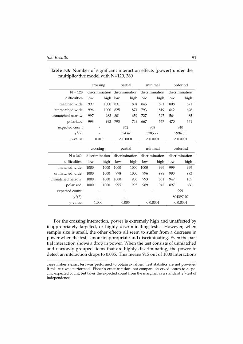
5.3. Results 91
Table 5.3: Number of significant interaction effects (power) under themultiplicative model with N=120, 360
crossing
N = 120 discrimination
difficulties low high
matched wide 999 1000
unmatched wide 996 1000
unmatched narrow 997 983
polarized 998 993
expected count -
χ2(7) -
p-value 0.010
partial
discrimination
low high
831 894
825 874
801 659
793 749
862
554.47
< 0.0001
minimal
discrimination
low high
845 891
793 819
727 397
667 557
868
3385.77
< 0.0001
orderind
discrimination
low high
808 871
642 696
564 85
470 361
840
7994.55
< 0.0001
crossing
N = 360 discrimination
difficulties low high
matched wide 1000 1000
unmatched wide 1000 1000
unmatched narrow 1000 1000
polarized 1000 1000
expected count -
χ2(7) -
p-value 1.000
partial
discrimination
low high
1000 1000
998 1000
1000 986
995 995
-
-
0.005
minimal
discrimination
low high
1000 999
996 998
993 851
989 942
-
-
< 0.0001
orderind
discrimination
low high
999 999
983 993
947 167
897 686
999
804397.40
< 0.0001
For the crossing interaction, power is extremely high and unaffected byinappropriately targeted, or highly discriminating tests. However, whensample size is small, the other effects all seem to suffer from a decrease inpower when the test is more inappropriate and discriminating. Even the par-tial interaction shows a drop in power. When the test consists of unmatchedand narrowly grouped items that are highly discriminating, the power todetect an interaction drops to 0.085. This means 915 out of 1000 interactions
cases Fisher’s exact test was performed to obtain p-values. Test statistics are not providedif this test was performed. Fisher’s exact test does not compare observed scores to a spe-cific expected count, but takes the expected count from the marginal as a standard χ2-test ofindependence.

92 5. How to Avoid Misinterpretation of Interaction Effects
were overlooked. This unsettling result is less pronounced in the large sam-ple. For the partial interaction the decrease in power is no longer significant.Of course, this is not unexpected, since an increased sample size improvespower. Although the detrimental effect is smaller in the minimal and par-tial interaction, these findings are nonetheless interesting, since according toLoftus (1978), these types of interactions should be robust against nonlinearmonotonic transformation of the scale.
To give an idea of what the observed effects actually look like, the ob-served means were averaged over iterations and plotted in Figure 5.4. Thesmall and moderate main effects and the order-independent interaction plot-ted for the observed means obviously look different compared to the effectsplotted for the latent means in Figure 5.2.
Figure 5.4: Mean observed effects for unmatched narrow test with highdiscrimination and sample size 120. Annotated using the alcohol ex-ample for illustrative purposes
no effects
Lemonade Alcohol
04
81
2
Sum
Score
female
male
one main effect
Lemonade Alcohol
04
81
2
Sum
Score
small main effects
Lemonade Alcohol
04
81
2
Sum
Score
moderate main effects
Lemonade Alcohol
04
81
2
Sum
Score
crossing interaction
Lemonade Alcohol
04
81
2
Sum
Score
partial interaction
Lemonade Alcohol
04
81
2
Sum
Score
minimal interaction
Lemonade Alcohol
04
81
2
Sum
Score
order−independent interaction
Lemonade Alcohol
04
81
2
Sum
Score
5.3. Results 93
5.3.3 Distributional Shape of Observed and Box-Cox TransformedScores
It seems highly likely that inferential error is indicated by non-normal ornon-symmetric sample distributions. Therefore the assumptions of normal-ity and homogeneity of variances were tested for all combinations of effecttype, sample size, discrimination and difficulty. Skewness and kurtosis coef-ficients were also calculated. Tests and coefficients were determined for boththe original observed scores and the Box-Cox transformed observed scores.Figure 5.5 shows the number of significant Shapiro-Wilks and Levene’s testsand the mean skewness and kurtosis. The results based on the latent abili-ties are provided as a base rate. Since the same pattern emerged for differ-ent types of effects and sample sizes, the results were collapsed over thesefactors. Unfortunately this means that tests of normality and homogeneityof variances cannot be used to distinguish between situations that are moreat risk for inferential error (e.g. between small and moderate main effects).However, violation of these tests is associated with inappropriate tests ingeneral.
It is interesting to note that virtually all inferential errors could be avoidedby considering uninterpretable those effects that coincided with violation ofnormality or homogeneity of variances. Of course this leads one to err onthe side of caution by also discarding a large proportion of valid inferences.Inferential error and violation of normality and homogeneity are not per-fectly correlated however. Data are not provided due to limited space, butan informal inspection of the simulated data showed that inferential errorscan be associated with samples that do not violate assumptions of normalityand homogeneity, but only if the mismatch between items and abilities is lessextreme.
As for skewness and kurtosis, the sum scores were skewed to the leftwith a longer right tail in all cases, but extremely so and moreover highlypeaked (leptokurtotic) when discrimination was high and test difficulty wasunmatched and narrowly targeted or polarized. As expected, the Box-Coxtransformed sum scores show much lower rejection of normality and het-erogeneity of variance assumptions and much less extreme skewness andkurtosis.

94 5. How to Avoid Misinterpretation of Interaction Effects
Figure 5.5: Rejection rate for Shapiro-Wilks and Levene’s test and stan-dard Skewness and Kurtosis coefficients for sum scores, Box-Coxsum scores and latent scores
Normality
matched unmatched unmatched polarizedwide wide narrow
low high low high low high low high
02
00
40
06
00
80
0
Homogeneity
matched unmatched unmatched polarizedwide wide narrow
low high low high low high low high
02
00
40
06
00
80
0
Skewness
matched unmatched unmatched polarizedwide wide narrow
low high low high low high low high
−0
.50
.51
.52
.5
Kurtosis
matched unmatched unmatched polarizedwide wide narrow
low high low high low high low high
−1
01
23
45
SumBox−CoxLatent
5.3.4 Box-Cox Transformed Scores and Group Differences in Reli-ability
A final goal of this study was to see whether a normalizing transformationcould be used to approximate the latent scores and minimize inferential er-ror. Therefore ANOVAs were also performed on the Box-Cox transformedscores. Tables 5.4 and 5.5 show the main results for the Box-Cox trans-formed sum scores when true effects were generated using the additive andmultiplicative model respectively. The results show the elevated risk of in-ferential error for tests that are ill-targeted, provide poor scale coverage, and
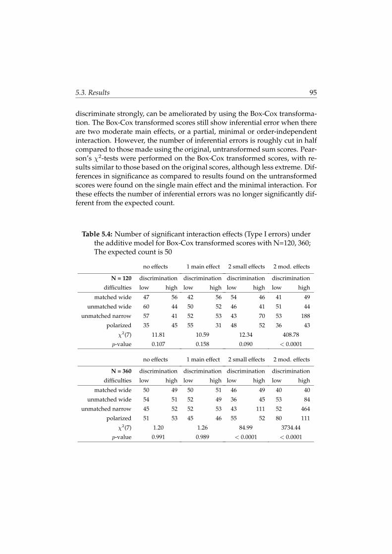
5.3. Results 95
discriminate strongly, can be ameliorated by using the Box-Cox transforma-tion. The Box-Cox transformed scores still show inferential error when thereare two moderate main effects, or a partial, minimal or order-independentinteraction. However, the number of inferential errors is roughly cut in halfcompared to those made using the original, untransformed sum scores. Pear-son’s χ2-tests were performed on the Box-Cox transformed scores, with re-sults similar to those based on the original scores, although less extreme. Dif-ferences in significance as compared to results found on the untransformedscores were found on the single main effect and the minimal interaction. Forthese effects the number of inferential errors was no longer significantly dif-ferent from the expected count.
Table 5.4: Number of significant interaction effects (Type I errors) underthe additive model for Box-Cox transformed scores with N=120, 360;The expected count is 50
no effects
N = 120 discrimination
difficulties low high
matched wide 47 56
unmatched wide 60 44
unmatched narrow 57 41
polarized 35 45
χ2(7) 11.81
p-value 0.107
1 main effect
discrimination
low high
42 56
50 52
52 53
55 31
10.59
0.158
2 small effects
discrimination
low high
54 46
46 41
43 70
48 52
12.34
0.090
2 mod. effects
discrimination
low high
41 49
51 44
53 188
36 43
408.78
< 0.0001
no effects
N = 360 discrimination
difficulties low high
matched wide 50 49
unmatched wide 54 51
unmatched narrow 45 52
polarized 51 53
χ2(7) 1.20
p-value 0.991
1 main effect
discrimination
low high
50 51
52 49
52 53
45 46
1.26
0.989
2 small effects
discrimination
low high
46 49
36 45
43 111
55 52
84.99
< 0.0001
2 mod. effects
discrimination
low high
40 40
53 84
52 464
80 111
3734.44
< 0.0001

96 5. How to Avoid Misinterpretation of Interaction Effects
Table 5.5: Number of significant interaction effects (power) under themultiplicative model for Box-Cox transformed scores with N=120,360
crossing
N = 120 discrimination
difficulties low high
matched wide 999 1000
unmatched wide 998 1000
unmatched narrow 999 996
polarized 997 1000
expected count -
χ2(7) -
p-value 0.429
partial
discrimination
low high
825 896
826 864
807 778
800 836
860
144.53
< 0.0001
minimal
discrimination
low high
848 899
838 885
824 649
759 782
874
704.04
< 0.0001
orderind
discrimination
low high
806 883
768 914
767 327
685 730
844
2469.44
< 0.0001
crossing
N = 360 discrimination
difficulties low high
matched wide 1000 1000
unmatched wide 1000 1000
unmatched narrow 1000 1000
polarized 1000 1000
expected count -
χ2(-) -
p-value 1.000
partial
discrimination
low high
1000 1000
998 1000
999 996
996 1000
-
-
0.315
minimal
discrimination
low high
1000 999
998 1000
998 988
997 999
-
-
0.118
orderind
discrimination
low high
1000 999
995 1000
997 751
982 990
-
-
< 0.0001
5.4 Assessing Risk
Results from previous studies by Dolan (1994), Loftus (1978), Davison andSharma (1990), Embretson (1996) and Kang and Waller (2005) can be com-bined with current results to better identify potential high risk research set-tings for typical experimental studies. The flowchart displayed in Figure 5.6provides a decision tree that addresses the most important factors in an ef-ficient order. Assuming the dependent variable is measured with a ques-tionnaire or test, the first consideration is the number of response categories.When items are polytomous, with five to seven or more response categories,
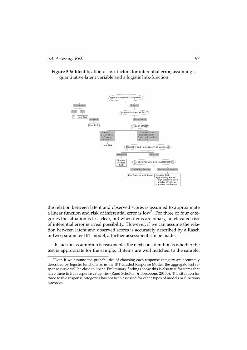
5.4. Assessing Risk 97
Figure 5.6: Identification of risk factors for inferential error, assuming aquantitative latent variable and a logistic link-function
Type of Response Categories?
Polytomous
3-4
?
5+
Low Risk
Binary*
Appropriateness of Test?
Matched
Low Risk
Mismatched
Type of Effect?
No Effects, 1 Main Effect or Crossing Interaction
Low Risk
2 Main Effects or Partial/Minimal/ Order-Independent Interaction
Normality and Homogeneity of Variances?
Accepted
Slightly Elevated
Risk
Rejected
Results after Box-Cox transformation?
Conflicting Results
Use Transformed Scores
Concurrent Results
Elevated Risk, Aggravating Factors: - high discrimination - greater effect size - greater test length
the relation between latent and observed scores is assumed to approximatea linear function and risk of inferential error is low7. For three or four cate-gories the situation is less clear, but when items are binary, an elevated riskof inferential error is a real possibility. However, if we can assume the rela-tion between latent and observed scores is accurately described by a Raschor two-parameter IRT model, a further assessment can be made.
If such an assumption is reasonable, the next consideration is whether thetest is appropriate for the sample. If items are well matched to the sample,
7Even if we assume the probabilities of choosing each response category are accuratelydescribed by logistic functions as in the IRT Graded Response Model, the aggregate test re-sponse curve will be close to linear. Preliminary findings show this is also true for items thathave three to five response categories (Zand Scholten & Borsboom, 2010b). The situation forthree to five response categories has not been assessed for other types of models or functionshowever.
98 5. How to Avoid Misinterpretation of Interaction Effects
risk of inferential error is low. However, when the items are very difficultor very easy and provide poor coverage of the ability scale, inferential er-ror could occur (Kang & Waller, 2005). If this is the case, the next step isto consider the type of effect, since not all effects are equally vulnerable toinferential error.
If the group means show no effects, one main effect or a crossing inter-action, risk of inferential error is low. In contrast, if the group means showan order-independent interaction or two main effects, caution is warranted(Loftus, 1978). Due to the combined effect of nonlinear transformation andsampling error, the same applies to partial and minimal interactions, albeitto a lesser extent. Fortunately, when tests show that normality and homo-geneity of variances can be accepted, risk of inferential error is only slightlyelevated. However, when normality or homogeneity have to be rejected, thiscould be due to a distorting effect of the nonlinear relation. Scores can betransformed to normalize the data, by using a procedure such as the Box-Cox transformation.
When results from an analysis based on Box-Cox transformed scores op-pose those based on the original scores, the transformed scores can be usedas an approximation of the latent ability values, similar to latent ability esti-mates obtained from IRT modeling. When results concur with those basedon the original scores, we have to accept that the risk of inferential error isstill present, although its magnitude is hard to assess. Some factors that canbe considered are effect size, test length, item discrimination and sample size.Effect size and test length increase the risk of inferential error as they growlarger. For sample size, the same applies if the true effect is additive, but ifa true interaction is present, a larger sample size is beneficial and decreasesthe risk of inferential error. Of course, in practice, the true effect is unknown,so that the impact of sample size is hard to determine. An effect that is morereadily interpretable is the effect of item discrimination. For almost all ef-fects low item discrimination can greatly ameliorate the risk of inferentialerror. A test with moderate item discrimination is only at risk for inferentialerror when effect size is large and the effect consists of an order-independentinteraction or two main effects.

5.5. Discussion 99
5.5 Discussion
Our results show that there is a substantial risk of making inferential errorsconcerning interaction effects under conditions that are typical for many ex-perimental studies in psychology. This danger is only clear and present how-ever, when a test with dichotomous items is employed that is inappropriatelydifficult (or easy). Under these conditions, the number of spurious interac-tions or Type I errors increased sharply when the true effects consisted of twomoderate main effects. Increasing item discrimination, which corresponds toimproving the reliability of the test, only exacerbated the problem. The situ-ation was even more serious when interactions were actually present on thelatent level. More than 90 percent of the latent order-independent interac-tions was overlooked when observed scores on an ill-targeted test with poorability scale coverage and high discrimination. Of course we chose an ex-tremely difficult test to better illustrate the problem, but it is apparent thatmismatched tests can cause serious difficulties for experimental researchers.
The rejection rate of the tests of normality and homogeneity of variancesincreased when the test was inappropriate for the sample. This result is notunexpected. When a test is inappropriate, group means will tend to be moreextreme, resulting in ceiling or floor effects that are associated with skewedsample distributions and reduced variance. The skewness and kurtosis co-efficients underlined this. Unfortunately, these results are uniformly foundfor all types of effects. This means rejection of normality and equal varianceassumptions is linked to test inappropriateness, but cannot be used to differ-entiate between situations that are less or more at risk for inferential error.
Our results replicate earlier findings that suggest appropriate coverageof the ability sample is essential in guarding against invalid inference con-cerning interaction effects. This means that where possible, tests need tobe psychometrically sound, consisting of a moderate number of items, withmoderate item discrimination and item difficulties that are targeted at themean ability that is expected in the sample. In other words, items need tobe selected that produce a test characteristic curve that is maximally linear.It is interesting to note that actions to improve the internal and external va-lidity of research findings that are generally considered good practice, suchas increasing effect size, sample size, and test length, can be highly counter-productive when it comes to mitigating the risk of inferential errors.

100 5. How to Avoid Misinterpretation of Interaction Effects
But what if we are unable to use appropriate tests? Applying a Box-Coxtransformation to the observed scores resulted in less Type I errors under theadditive model and higher power to detect significant interactions under themultiplicative model. This transformation also improves rejection rates fortests of normality and homogeneity of variances. Skewness and kurtosis arealso much less extreme, which is to be expected of a transformation that isaimed at normalizing the data. Thus it seems that a Box-Cox transformationcan be used to kill two birds with one stone. Both statistical test assumptionsof normality and equal variances will be met more often, and the risk ofinferential errors is minimized.
In fact, the Box-Cox transformation can be viewed as an attempt to ap-proximate the latent values, which we assume to be distributed normally,without actually having to model the latent variable. Of course IRT mod-eling or generalized linear mixed modeling could provide a more elegantsolution to the problem of inferential error raised here, but since such meth-ods are not always available it is important to have an alternative way ofdealing with the risk of inferential error.
We have narrowed down potential problem situations to settings with in-appropriate tests that use dichotomous items, showing either minimal, par-tial or order-independent interactions, or two main effects. This reductioncomes at the cost of several additional assumptions. The most importantof these assumptions concerns the specification of the relation between thelatent and observed variable. We have chosen the two-parameter model be-cause it is simple and has the monotone likelihood ratio property, whichentails that the items result in a consistent ordering of persons abilities basedon the sum score. Although these models perhaps form an oversimplifiedrepresentation of the relation between latent and observed level, some sortof logistic-type function seems plausible. Other models can be consideredthat introduce more parameters that model characteristics such as guessingor slippage, for example. The effect of additional parameters on the linearityof the test response curve could provide more insight into our understandingof the risk of inferential error.

Chapter 6
The Interpretation of Interactions Based onPolytomous Items
Misinterpretation is the most deadly of human sins.
Lester del Rey
Abstract
Inferences about interactions can arbitrarily depend on choice of measurementscale. Inferential error can occur when ordinal observed scores, assumed torepresent an underlying quantitative variable, are related to the latent valuesnonlinearly, as is the case in Item Response Theory (IRT) models. Using sev-eral IRT models to simulate data, the risk of inferential error for interactionseffects based on dichotomous data was assessed to be high when the test wasinappropriate targeted and strongly discriminating for large and small sam-ple sizes and several types of interaction effects (Embretson, 1996; Kang &Waller, 2005; Zand Scholten & Borsboom, 2010a). We extended this work forpolytomous items using the Graded Response Model (GRM) to simulate datain a small sample, standard ANOVA setting. We also considered the effect ofincreasing the number of response categories on the risk of inferential error forseveral types of interaction effects. Results show that inferential error for in-appropriately targeted, highly discriminating test is present in data simulatedusing the GRM. An increase in number of response categories is associatedwith a decrease in inferential error. Box-Cox transformed observed scores showacceptable levels of inferential error.
102 6. The Interpretation of Interactions Based on Polytomous Items
6.1 Introduction
The truth value of inferences based on ‘inadmissible’ statistics, such asparametric tests performed on ordinal data, can depend on the arbi-
trary choice of numerical scale1. A conclusion that reverses with a changein scale, even though both numerical assignments represent the underlyingordinal relations equally well, is meaningless and therefore highly undesir-able. This is why basic textbooks teach social scientists that performing at-test or ANOVA on ordinal data is, strictly speaking, not allowed (Winer,1971; Shaughnessy et al., 2000; Breakwell et al., 2003). In the same breathhowever, such textbooks often downplay the actual risk of making an infer-ential error based on inadmissible statistics, by stating that in practice thesetests can be performed without qualm, since ordinal data often provide a suf-ficiently close approximation to the interval level of measurement. Whetherthis assurance is warranted however has received relatively little attention.
A conclusion concerning two group means based on ordinal scores can bereversed by a transformation according to a monotonically increasing func-tion (leaving order intact) that stretches or condenses a certain part of thescale. This can bring the means closer together or further apart, or evenchange their order. Some interesting examples are provided by Townsendand Ashby (1984), Hand (2004) and Zand Scholten and Borsboom (2010a).Such a change in conclusion can only be arrived at under certain conditionshowever. When the sample distributions in the two groups have the sameshape, they are stochastically ordered, which means it is impossible to finda monotonically increasing function that will change the inference based onthese scores (Davison & Sharma, 1988). Early simulation research into theeffect of several nonlinear transformations on sensitivity to inferential errorin the t-test showed the risk was small (Baker et al., 1966). The same unfor-tunately does not apply to more complicated comparisons of group meanshowever.
A more complicated type of comparison that runs a much higher riskof producing inferential errors is the interaction effect considered in stan-dard factorial designs. Loftus (1978) was the first to point out that when weassume the data represent a latent quantitative variable and the relation to
1The next six paragraphs treat the concept of admissible statistics similarly to previouschapters and may therefore be skipped if the reader so wishes.
6.1. Introduction 103
the ordinal observed scores is some unknown nonlinear function, then cer-tain interaction effects are at risk for inferential error while others are not.When the effect consists of no effects, one main effect, a crossing interactionor what we term a partial and minimal interaction (see Figure 6.1), then itis impossible to find a transformation that will change these effects. How-ever, when there are two main effects or an order-independent interaction(see Figure 6.1) it is possible to find a transformation that will change theformer into the latter or vice versa, thereby causing an inferential error.
It is important to note that Loftus (1978) did not take measurement errorinto account, and therefore considered equal means, which cannot be madeto differ by any one-to-one transformation, safe from inferential error. Inpractice, two or more means will never be exactly equal, leaving the risk ofinferential error undetermined. In order to narrow down the conditions thatpresent a risk of inferential error, an effort was made to investigate whetherstandard ANOVA assumptions of normality and homogeneity of variances,resulting in equivalently shaped sample distributions, would preclude infer-ential error for a two-by-two interaction design (Davison & Sharma, 1990).Unfortunately this attempt was not successful.
Embretson (1996) was the first to employ Item Response Theory (IRT)modeling to investigate a specific type of relation between assumed quan-titative latent values and ordinal observed scores. Data were simulated ac-cording to the Rasch model, which results in a logistic-type relation betweenlatent and observed scores. Parameters such as item difficulty and discrim-ination, that influence the linearity of this relation, were manipulated togauge the risk of inferential error, and to assess the usefulness of IRT abil-ity estimates to mitigate inferential error. Only when the test was inappro-priately targeted to the sample, which corresponds to a less linear function,did spurious interactions occur. Latent ability estimates were successfullyused to lessen the risk of inferential error. Extension of this line of investiga-tion showed similar results for data simulated using the 2-Parameter Logistic(2PL) IRT model (Kang & Waller, 2005).
Simulation research based on IRT modeling constitutes a great step for-ward in fleshing out the conditions associated with an elevated risk of infer-ential error. However, this research (Embretson, 1996; Kang & Waller, 2005)uses a Moderated Multiple Regression (MMR) approach with large samplesize, only considers the order-independent interaction and presents IRT abil-

104 6. The Interpretation of Interactions Based on Polytomous Items
Figure 6.1: Four additive and multiplicative types of effects, categorizedaccording to group order restraints
no effects
Control Treatment
−1
01
Su
m S
co
re
level 1
level 2
one main effect
Control Treatment
−1
01
Su
m S
co
re
small main effects
Control Treatment
−1
01
Su
m S
co
re
moderate main effects
Control Treatment
−1
01
Su
m S
co
re
crossing interaction
Control Treatment
−1
01
Su
m S
co
re
partial interaction
Control Treatment
−1
01
Su
m S
co
re
minimal interaction
Control Treatment
−1
01
Su
m S
co
re
order−independent interaction
Control Treatment
−1
01
Su
m S
co
re
ity estimation as a solution to the problem of inferential error. Zand Scholtenand Borsboom (2010a) approach the problem from the perspective of exper-imental researchers who often only have access to small sample sizes andfixed effect designs. Estimation of latent abilities using IRT is not an optionin this case. IRT modeling can still be useful in this context however, since itallows us to make coherent assumptions about the function that relates latentand observed scores. Using the 2PL model to simulate data, Zand Scholten

6.2. Simulation Study 105
and Borsboom (2010a) showed that for small to moderate sample sizes too,the risk of inferential error for inappropriately targeted tests is sizeable. In-ferential error occurred for order-independent interactions, but also for othertypes of effects, namely two moderate main effects, as well as the partial andminimal interaction, albeit to a lesser extent. An alternative solution to IRTestimation of latent abilities was found in a normalizing transformation: Theuse of normally transformed scores showed a marked decrease in inferentialerror.
A natural extension of previous research employing IRT modeling is toinvestigate the risk of inferential error for tests that consist of polytomousitems. When more response categories are available allowing persons to pro-vide a more fine-grained response, it is possible that the relation betweenassumed quantitative latent values and ordinal observed scores will becomemore linear. To investigate this for the MMR, large sample size case, Morse(submitted) simulated data according to the Graded Response Model (GRM)using five response categories. As in previous research, inferential error isagain present for inappropriate tests and can be mitigated using ability esti-mates. The risk of inferential error is somewhat lower however.
In the current paper we aim to extend this research for the small samplesize, standard ANOVA case. As before, we considered several other typesof interaction effects besides the order-independent interaction. We also in-vestigated the effect of different numbers of response categories. As the pos-sibility to differentiate one’s response increases, the relation between latentand observed is expected to become more linear, resulting in less inferentialerror. We were interested to see whether an increase in response categoriescould reduce the risk of inferential error to acceptable levels. We also con-sidered the effect of a normalizing transformation on the risk of inferentialerror, expecting an error decrease. In the next section a general descriptionof the simulation is provided, followed by a more elaborate treatment in themethod section.
6.2 Simulation Study
Our goal was to asses the risk of inferential errors based on Likert-scale dataunder conditions typical for experimental studies. Therefore a two-by-twofixed effects design with small sample size was chosen. The types of effects
106 6. The Interpretation of Interactions Based on Polytomous Items
considered are the crossing, partial, minimal and order-independent inter-action and corresponding main effects depicted in Figure 5.2. Ability valueswere generated producing these effects at the latent level. These values weretransformed into observed scores using the Graded Response Model, one ofthe simplest polytomous IRT models available. A test of moderate to shortlength was simulated. The effect of test appropriateness was investigated byvarying item discrimination and response category threshold values, whichcorrespond to item difficulty in the dichotomous case.
The effect of test appropriateness on inferential validity was assessed us-ing data that were simulated repeatedly for each combination of factors. Thelatent scores and the observed scores were subjected to ANOVAs. A dis-crepancy between the number of significant interactions obtained from theobserved scores and those obtained from the latent scores indicates infer-ential error. Descriptive statistics and a normalizing transformation of theobserved scores were considered, to see if these could signal or mitigate anelevated risk of inferential error. The exact simulation setup is discussed inmore detail below.
6.3 Method
6.3.1 Simulation of Latent Scores
We simulated an experimental study with two independent factors F1 andF2, each with two levels, and one dependent response variable. The simula-tion consisted of two steps. In the first step latent ability values were gener-ated according to the model θ = t+ w1 · F1 + w2 · F2 + w12 · F1 · F2, where twas randomly sampled from a standard normal distribution. Factors F1 andF2 indicate assignment to one of two levels (contrast coded -1 or 1) on eachfactor, and w1, w2 and w12 indicate the weights used to determine main andinteraction effects on the latent level. Sample size was set at 120, resulting ingroup sizes of 30.

6.3. Method 107
6.3.2 Simulation of Observed Scores
In the second step of the simulation, latent scores were transformed into sumscores. Item responses were generated according to the Graded ResponseModel, which models item responses to more than two categories using a lo-gistic function with an item discrimination parameter and between-categorythreshold parameters. The between-category thresholds are introduced foreach item i in order to obtain response probabilities for each ofXi categories.This means there are Mi = Xi−1 thresholds for item i. Given the latent abil-ity, the probability of a response falling in or above category x on item i is:
p∗ijx(θ) =exp(αi(θj − βik))
1 + exp(αi(θj − βik))
This equation produces what is called an operating curve, where θj denotesthe latent ability of person j, simulated in step one. βik denotes the abilityvalue associated with a .50 probability of responding above threshold k foritem i, where x = k = 1, 2, . . .Mi. α denotes the item discrimination ofitem i, which is the same for all operating curves 2. The probability pijx(θ)for person j of answering in response category x on item i, is obtained bysubtraction:
pijx(θ) = p∗ijx(θ)− p∗ij(x+1)(θ)
Where x = 0, 1, . . . Xi, and where pij0(θ) = 1, and pij(Xi+1)(θ) = 0 by defi-nition. The resulting response category probabilities were then recoded intoscores between 1 and Xi. This was achieved separately for each person oneach item, by drawing from a multinomial distribution where the responsecategories formed the classes and the response category probabilities of theperson formed the class probabilities. Finally the item responses were addedfor each person, resulting in sum scores.
6.3.3 Expected Interaction Effects
Either an additive model or a multiplicative model was used to simulate thelatent ability values. The additive model contained no interaction term by
2Although item discrimination was the same for all items in a particular simulated test,discrimination was treated as a factor in the simulation study and was set to either a high orlow value. We therefore retain the subscript.
108 6. The Interpretation of Interactions Based on Polytomous Items
setting the weight w12 to zero. Any interaction on the latent level under thismodel will be due to sampling error. The number of significant interactionson the simulated sum scores was therefore expected to be small (low Type Ierror rate). A significant interaction under this model is spurious and indi-cates inferential error. Under the multiplicative model, an interaction termwas introduced by setting the weight w12 to a non-zero value. Latent abil-ities generated under this model will show significant interactions, exceptfor sampling error. A high number of significant interactions are thereforeexpected on the simulated sum scores (low Type II error rate, high power).A non-significant interaction effect under the multiplicative model indicatesinferential error.
6.3.4 Types of Simulated Effects
The effects displayed in Figure 6.1 were simulated by choosing the followingcombinations of weights w1, w2 and w12. The weights (0.0, 0.0, 0.5) produceno main effects (additive model) or a fully crossing interaction (multiplica-tive model). The weights (0.0,−0.5, 0.3) produce one moderate main effect(additive model), or a partial interaction (multiplicative model). The weights(0.3,−0.3, 0.3) result in two small main effects (additive model), or a minimalinteraction (multiplicative model). The weights (0.5,−0.5, 0.3) produce twomoderate main effects (additive model), or an order-independent interaction(multiplicative model).
6.3.5 Test Characteristics
The number of items was set to 15, to simulate a moderately short test. Itemdiscrimination was low (α = 1) or high (α = 4). Item response thresh-old values were based on item difficulty values used in a previous study(Zand Scholten & Borsboom, 2010a), where differently grouped sets of itemdifficulties were compared. In the first case the item difficulties matchedthe distribution of abilities and were spaced equidistantly over a wide rangeof the ability scale, from -2.5 and 2.5, resulting in an appropriately targetedtest. In the second case item difficulties were mismatched to the distributionof abilities and equidistantly over a narrow range, between 0.875 and 1.625,resulting in an inappropriately targeted test. Of course these item difficul-
6.3. Method 109
ties pertain to dichotomous items and need to be transformed into responsethreshold categories. The number of response categories varied from threeto seven categories. Threshold values were chosen around the item difficultyof each item. For example, for three categories the lower threshold was set to(difficulty - 1.00) and the upper threshold was set to (difficulty + 0.00). Thethreshold values were chosen around the item difficulty as follows for eachnumber of categories:
• three categories: -1.00 and 0.00
• four categories: -1.25, -0.50 and 0.25
• five categories: -1.50, -0.75, 0.00 and 0.50
• six categories: -1.75, -1.25, -0.25, 0.25 and 0.75
• seven categories: -2.00, -1.50, -0.75, 0.00, 0.50 and 1.00
6.3.6 Descriptive Statistics and Tests
The current study consisted of 160 levels: 2 (additive/multiplicative model)× 4 (choice of weights resulting in main/interaction effects) × 2 (item dif-ficulty sets used to generate thresholds) × 2 (item discrimination) × 5 (re-sponse categories). Data were simulated a 1000 times for each combinationof levels. For each simulation run, an ANOVA was performed on the latentand ‘observed’ scores. The significance level was set at 0.05. To see if sig-nificant interactions exceeded the expected number, Pearson χ2-tests wereperformed. These tests are not to be confused with the standard χ2-test ofindependence. Due to the considerable number of tests, a Bonferroni correc-tion was applied, resulting in a significance level of 0.001.
Both the observed and latent scores were subjected to Shapiro-Wilks testof normality and Levene’s test of homogeneity of variances. Skewness andkurtosis coefficients were also calculated. Non-normality and heterogeneityof variances were expected in the groups with the lowest means, due to afloor effect. A normalizing transformation could provide a way to mitigatethe distorting effect of the non-linear relation between latent and observedscores. Normalization could be considered an approximation to the latentscores without having to resort to modeling. Sum scores were thereforetransformed according to a Box-Cox transformation. All descriptive statis-
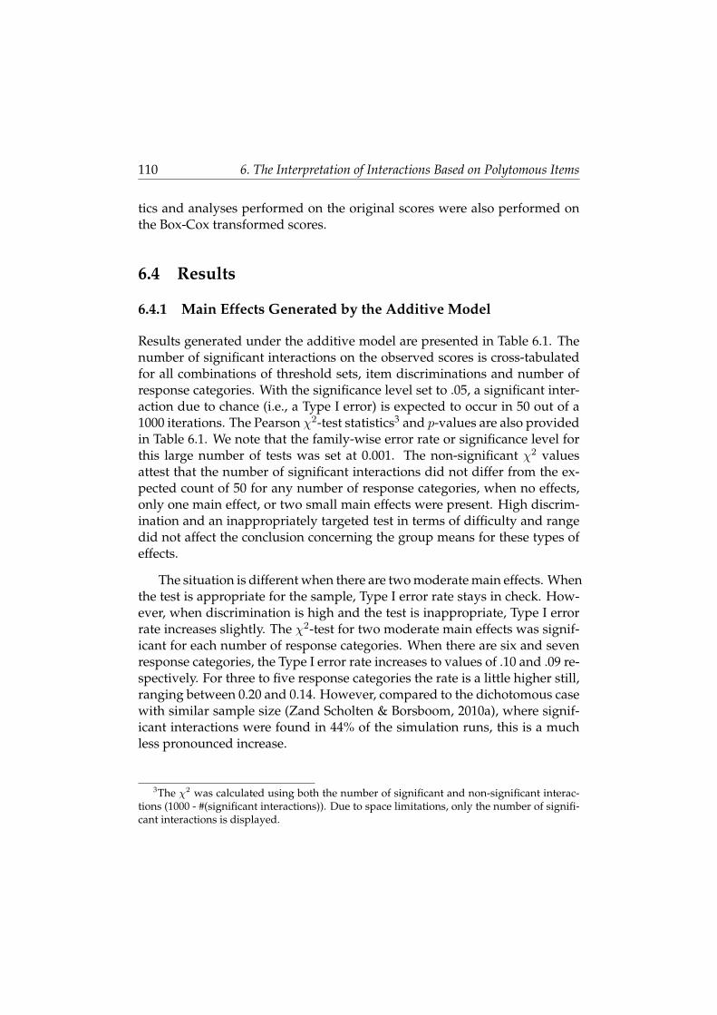
110 6. The Interpretation of Interactions Based on Polytomous Items
tics and analyses performed on the original scores were also performed onthe Box-Cox transformed scores.
6.4 Results
6.4.1 Main Effects Generated by the Additive Model
Results generated under the additive model are presented in Table 6.1. Thenumber of significant interactions on the observed scores is cross-tabulatedfor all combinations of threshold sets, item discriminations and number ofresponse categories. With the significance level set to .05, a significant inter-action due to chance (i.e., a Type I error) is expected to occur in 50 out of a1000 iterations. The Pearson χ2-test statistics3 and p-values are also providedin Table 6.1. We note that the family-wise error rate or significance level forthis large number of tests was set at 0.001. The non-significant χ2 valuesattest that the number of significant interactions did not differ from the ex-pected count of 50 for any number of response categories, when no effects,only one main effect, or two small main effects were present. High discrim-ination and an inappropriately targeted test in terms of difficulty and rangedid not affect the conclusion concerning the group means for these types ofeffects.
The situation is different when there are two moderate main effects. Whenthe test is appropriate for the sample, Type I error rate stays in check. How-ever, when discrimination is high and the test is inappropriate, Type I errorrate increases slightly. The χ2-test for two moderate main effects was signif-icant for each number of response categories. When there are six and sevenresponse categories, the Type I error rate increases to values of .10 and .09 re-spectively. For three to five response categories the rate is a little higher still,ranging between 0.20 and 0.14. However, compared to the dichotomous casewith similar sample size (Zand Scholten & Borsboom, 2010a), where signif-icant interactions were found in 44% of the simulation runs, this is a muchless pronounced increase.
3The χ2 was calculated using both the number of significant and non-significant interac-tions (1000 - #(significant interactions)). Due to space limitations, only the number of signifi-cant interactions is displayed.
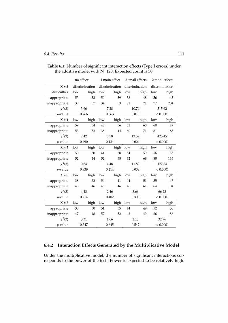
6.4. Results 111
Table 6.1: Number of significant interaction effects (Type I errors) underthe additive model with N=120; Expected count is 50
no effects
X = 3 discrimination
difficulties low high
appropriate 53 53
inappropriate 39 57
χ2(3) 3.96
p-value 0.266
X = 4 low high
appropriate 59 54
inappropriate 53 53
χ2(3) 2.42
p-value 0.490
X = 5 low high
appropriate 50 50
inappropriate 52 44
χ2(3) 0.84
p-value 0.839
X = 6 low high
appropriate 38 52
inappropriate 43 46
χ2(3) 4.48
p-value 0.214
X = 7 low high
appropriate 38 50
inappropriate 47 48
χ2(3) 3.31
p-value 0.347
1 main effect
discrimination
low high
50 59
34 53
7.28
0.063
low high
43 56
38 44
5.58
0.134
low high
41 58
52 58
4.48
0.214
low high
54 41
48 46
2.46
0.482
low high
51 55
57 52
1.66
0.645
2 small effects
discrimination
low high
58 48
51 71
10.74
0.013
low high
51 60
60 71
13.52
0.004
low high
54 59
62 68
11.89
0.008
low high
44 51
46 61
3.66
0.300
low high
44 49
42 49
2.15
0.542
2 mod. effects
discrimination
low high
56 45
77 204
515.92
< 0.0001
low high
60 47
81 188
423.45
< 0.0001
low high
56 55
80 135
172.34
< 0.0001
low high
55 47
64 104
66.23
< 0.0001
low high
52 50
66 86
32.76
< 0.0001
6.4.2 Interaction Effects Generated by the Multiplicative Model
Under the multiplicative model, the number of significant interactions cor-responds to the power of the test. Power is expected to be relatively high.

112 6. The Interpretation of Interactions Based on Polytomous Items
Because power is influenced by effect size, and since effect size varies be-tween conditions, a reasonable expected count for each type of effect neededto be determined. Therefore the number of significant interactions on theappropriate, matched wide test, averaged over high and low discrimination,was used as a baseline for each type of effect. The number of significant in-teractions, expected counts and test results obtained under the multiplicativemodel4, are displayed in Table 6.2.
Power is very high and unaffected by an inappropriate test with highdiscrimination when the effect consists of a crossing interaction, no matterthe number of response categories. The same seems to apply to the partialinteraction. Although the χ2-test is significant for each number of responsecategories for this type effect, the drop in power is not very great and actu-ally goes up when discrimination is high. Overall differences between highand low discrimination are greater than differences between the appropri-ate and inappropriate test. For the minimal interaction a similar patternemerges when there are seven response categories. When there are threeto six response categories, the power dropped more than 10% if the test isinappropriate and discrimination is high versus low. The decreased powervaries between .68 at its worst and .83 at its best, increasing with the numberof response categories.
Compared to data generated under the additive model, this is nowherenear as extreme as in the dichotomous case, where power dropped to .40under otherwise comparable circumstances. For the order-independent in-teraction the situation is somewhat more serious. The number of significantinteractions is markedly lower for the inappropriate test compared to the ap-propriate test, especially when discrimination is high. Power varies between.38 and .74, once more increasing with the number of response categories.Compared to the dichotomous case however, the decrease is less impressive.With the same simulation generating dichotomous data, power dropped to.09 (!). We also see a change in direction of the effect of discrimination. High
4In several cases the expected count for non-significant interactions (not displayed in Ta-ble 6.2) was zero. In these cases the expected count was changed to 0.1. Another problemwas the occurrence of empty or very low cell counts for the non-significant columns. In thesecases Fisher’s exact test was performed to obtain p-values. Test statistics are not providedif this test was performed. Fisher’s exact test does not compare observed scores to a spe-cific expected count, but takes the expected count from the marginals as a standard χ2-test ofindependence.

6.4. Results 113
Table 6.2: Number of significant interaction effects (Type II er-rors/power) under the multiplicative model with N=120
crossing
X = 3 discrimination
difficulties low high
appropriate 998 1000
inappropriate 997 999
exp. count -
χ2(3), p-value - , 0.538
X = 4 low high
appropriate 997 1000
inappropriate 1000 1000
exp. count -
χ2(3), p-value - , 0.341
X = 5 low high
appropriate 1000 1000
inappropriate 997 999
exp. count -
χ2(3), p-value - , 0.736
X = 6 low high
appropriate 998 1000
inappropriate 999 1000
exp. count -
χ2(3), p-value - , 0.617
X = 7 low high
appropriate 996 1000
inappropriate 997 1000
exp. count -
χ2(3), p-value - , 0.072
partial
discrimination
low high
758 875
779 817
816
54.71, < 0.0001
low high
777 890
796 833
834
56.56, < 0.0001
low high
762 884
797 847
823
59.68, < 0.0001
low high
774 890
808 872
832
63.70, < 0.0001
low high
788 897
789 882
842
77.80, < 0.0001
minimal
discrimination
low high
770 902
710 682
836
352.32, < 0.0001
low high
790 892
754 730
841
187.65, < 0.0001
low high
794 906
752 765
850
181.18, < 0.0001
low high
801 916
752 800
858
174.11, < 0.0001
low high
802 904
771 833
853
98.30, < 0.0001
order-indep.
discrimination
low high
774 902
634 376
838
1939.16, < 0.0001
low high
802 912
612 440
857
1958.07, < 0.0001
low high
780 913
618 522
846
1272.64, < 0.0001
low high
795 911
653 661
853
666.65, < 0.0001
low high
815 913
717 741
864
353.52, < 0.0001
discrimination leads to lower power when the number of response categorieslies between three and five. For six or seven response categories, discrimina-tion does not seem to affect power in the ill-matched test.
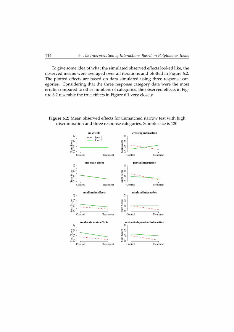
114 6. The Interpretation of Interactions Based on Polytomous Items
To give some idea of what the simulated observed effects looked like, theobserved means were averaged over all iterations and plotted in Figure 6.2.The plotted effects are based on data simulated using three response cat-egories. Considering that the three response category data were the mosterratic compared to other numbers of categories, the observed effects in Fig-ure 6.2 resemble the true effects in Figure 6.1 very closely.
Figure 6.2: Mean observed effects for unmatched narrow test with highdiscrimination and three response categories. Sample size is 120
no effects
Control Treatment
15
25
35
45
Sum
Score
level 1
level 2
one main effect
Control Treatment
15
25
35
45
Sum
Score
small main effects
Control Treatment
15
25
35
45
Sum
Score
moderate main effects
Control Treatment
15
25
35
45
Sum
Score
crossing interaction
Control Treatment
15
25
35
45
Sum
Score
partial interaction
Control Treatment
15
25
35
45
Sum
Score
minimal interaction
Control Treatment
15
25
35
45
Sum
Score
order−independent interaction
Control Treatment
15
25
35
45
Sum
Score

6.4. Results 115
6.4.3 Distributional Shape of Observed and Box-Cox TransformedScores
Deviations from normality and homogeneity of variances could indicate anincreased risk of inferential error. Normality and homogeneity of variancesassumptions were therefore tested for all combinations of effect types, num-ber of response categories, discrimination and threshold sets. Skewness andkurtosis coefficients were also calculated. All the tests and statistics were cal-culated for the original scores and the Box-Cox transformed observed scores.Figure 6.3 shows the number of significant Shapiro-Wilks and Levene’s testsand the mean skewness and kurtosis, averaged over effect type and numberof response categories.
Figure 6.3: Rejection rate for Shapiro-Wilks and Levene’s test and stan-dard Skewness and Kurtosis coefficients for sum scores, Box-Coxsum scores and latent scores
Normality
matched unmatchedwide narrow
low high low high
0200
600
1000
SumBox−CoxLatent
Homogeneity
matched unmatchedwide narrow
low high low high
0200
600
1000
Skewness
matched unmatchedwide narrow
low high low high
0.0
0.5
1.0
Kurtosis
matched unmatchedwide narrow
low high low high
−2.0
−1.5
−1.0
−0.5
0.0

116 6. The Interpretation of Interactions Based on Polytomous Items
The same results, based on the latent ability scores can serve as base ratecomparison. In general, violation of normality and homogeneity of vari-ances, and the presence of skewness and kurtosis are associated with in-appropriate tests that show high discrimination. The Box-Cox transformedsum scores do much better in this regard.
6.4.4 Box-Cox Transformed Scores and Group Differences in Reli-ability
A normalizing transformation could be used to approximate the latent scoreswithout having to resort to IRT modeling. An added benefit could be theminimization of inferential error. ANOVAs were therefore performed onthe Box-Cox transformed scores. Tables 6.3 and 6.4 show the main resultswhen data were simulated using the additive and multiplicative model re-spectively.
When compared to the results based on the original scores, it is clear thatthe Box-Cox transformation is beneficial in all cases. The Box-Cox trans-formed scores show no inferential error when there are two moderate maineffects. There is still some inferential error when there is a minimal or order-independent interaction but the number of inferential errors is roughly cut inhalf compared to the untransformed sum scores. Pearson’s χ2-tests were nolonger significant for any number of response categories on any of the typesof additive effects.
Table 6.4 shows that the partial, minimal and order-independent inter-actions still showed significant deviations from the expected count. This isprobably accounted for by the choice of expected number of significant in-teractions that was not ideal due to a relatively large overall difference insignificant interactions between low and high discrimination. Only for threeresponse categories in the minimal interaction case and three and four re-sponse categories in the order-independent interaction case, did the powerin the Box-Cox transformed scores drop more than 10%.

6.4. Results 117
Table 6.3: Number of significant interaction effects (Type I errors) un-der the additive model based on Box-Cox transformed scores withN=120; Expected count is 50
no effects
X = 3 discrimination
difficulties low high
appropriate 52 51
inappropriate 35 55
χ2(3) 5.37
p-value 0.147
X = 4 low high
appropriate 57 54
inappropriate 56 57
χ2(3) 3.16
p-value 0.368
X = 5 low high
appropriate 51 51
inappropriate 53 53
χ2(3) 0.42
p-value 0.936
X = 6 low high
appropriate 39 54
inappropriate 44 50
χ2(3) 3.64
p-value 0.303
X = 7 low high
appropriate 42 52
inappropriate 50 51
χ2(3) 1.45
p-value 0.693
1 main effect
discrimination
low high
49 61
32 50
9.39
0.025
low high
43 59
42 38
7.12
0.068
low high
41 60
51 64
7.96
0.047
low high
52 39
46 47
3.16
0.368
low high
49 55
62 55
4.11
0.250
2 small effects
discrimination
low high
57 50
54 48
1.45
0.693
low high
52 61
56 54
3.73
0.293
low high
49 53
49 51
0.25
0.969
low high
41 52
49 63
5.37
0.147
low high
40 46
45 48
3.05
0.384
2 mod. effects
discrimination
low high
48 37
62 64
10.8
0.013
low high
55 36
41 62
9.39
0.025
low high
50 44
63 46
4.65
0.199
low high
54 41
44 42
4.15
0.246
low high
51 44
56 40
3.64
0.303

118 6. The Interpretation of Interactions Based on Polytomous Items
Table 6.4: Number of significant interaction effects (Type II er-rors/power) under the multiplicative model based on Box-Coxtransformed scores with N=120
crossing
X = 3 discrimination
difficulties low high
appropriate 998 1000
inappropriate 998 1000
exp. count -
χ2(3), p-value - , 0.388
X = 4 low high
appropriate 1000 1000
inappropriate 998 999
exp. count -
χ2(3), p-value - , 1.000
X = 5 low high
appropriate 1000 1000
inappropriate 998 999
exp. count -
χ2(3), p-value - , 1.000
X = 6 low high
appropriate 998 1000
inappropriate 998 1000
exp. count -
χ2(3), p-value - , 0.366
X = 7 low high
appropriate 996 1000
inappropriate 997 1000
exp. count -
χ2(3), p-value - , 0.082
partial
discrimination
low high
754 877
771 838
816
67.10, < 0.0001
low high
777 894
796 852
834
62.24, < 0.0001
low high
759 886
805 867
823
70.88, < 0.0001
low high
771 892
808 885
832
76.59, < 0.0001
low high
784 897
790 890
842
85.67, < 0.0001
minimal
discrimination
low high
761 894
760 781
836
129.76, < 0.0001
low high
779 879
790 820
841
62.29, < 0.0001
low high
785 896
796 855
850
72.8, < 0.0001
low high
794 905
792 872
858
89.11, < 0.0001
low high
791 892
806 884
853
68.07, < 0.0001
order-indep.
discrimination
low high
741 877
749 665
838
359.32, < 0.0001
low high
763 870
701 747
857
370.79, < 0.0001
low high
752 881
727 820
846
191.11, < 0.0001
low high
760 871
760 864
853
141.5, < 0.0001
low high
778 881
804 883
864
99.11, < 0.0001

6.5. Discussion 119
6.5 Discussion
The results show that although a Likert-scaled, inappropriate test is still as-sociated with the risk of inferential error, this risk is much smaller than whendichotomous items are used. Furthermore, the risk decreases as the numberof response categories increases. When an inappropriate test is used thatconsists of items with seven response categories, the only problematic effecttypes are the order-independent interaction and the double main effect. ABox-Cox transformation provides a substantial improvement in these cases.
Of course it is important to note the limitations of our simulation setup.We chose a moderately short test and small sample size to simulate typicalconditions for an experimental setting. The inappropriateness of the test wasfixed by choosing specific values for the response category thresholds. Theaim was to facilitate comparison to previous results based on dichotomousresponses generated by the 2-parameter logistic IRT model. A drawback isthat we did not sample threshold values. The threshold values also resultedin extremely hard items, perhaps harder than we typically see in researchsettings where inappropriate tests cannot be avoided. This leads us to theoptimistic conclusion however, that the risk of inferential error in these ap-plied settings is therefore likely to be even smaller.
The Box-Cox transformation again proved to mitigate inferential error,as it did with dichotomous data. For all types of effects, for both types oftest appropriateness and for each number of response categories, the Box-Cox transformation reduced inferential error to acceptable levels. The onlyexception was when the true effect concerned an order-independent inter-action and the test was both inappropriate and consisted of a small numberof response categories. A normalizing transformation such as the Box-Coxtransformation seems to adequately approximate the latent scores in smallexperiments where IRT modeling is not an option.
Assuming data are generated according to a process that can accuratelybe described by the GRM, these data are only at risk for producing inferentialerrors under very specific circumstances. A sizable risk only occurs when thetest is highly inappropriate and the number of response categories is low.This does not mean that appropriately difficult items or a high number ofresponse categories will ensure that risk of inferential error will be absent.An important assumption here is that data behave as if generated by the

120 6. The Interpretation of Interactions Based on Polytomous Items
GRM. Whether this model provides an accurate description for many testsis questionable. Additional work needs to be done on more complex modelsthat a can be associated with much more non-linearity in the test responsecurve that ultimately determines the risk of inferential error.

Chapter 7
Discussion
The purpose of models is not to fit the data but tosharpen the question.
Samuel Karlin
7.1 Summary
The contribution of latent variable models to the determination of mea-surement level and the legitimacy of inferences is obviously controver-
sial. In this thesis I have tried to argue that latent variable models can beuseful in this respect but perhaps in a more modest way than some propose.In this final chapter first the conclusions and results of the preceding chap-ters will be summarized, followed by a more general conclusion about theusefulness of latent variables in addressing measurement level issues in psy-chology.
7.1.1 Measurement vs. Statistics
Chapter 2 of this thesis focused on Lord’s influential contribution to themeasurement-statistics debate (1953), which supplied most of the ammuni-tion in this fierce conflict. The theory of measurement levels and admissiblestatistics (Stevens, 1946) states that the choice of statistical test should dependon the measurement level associated with the data. This is because a statisticshould remain invariant, resulting in the same inference about the measuredproperty, under all structure-preserving transformations. Lord presented afictional example where an inadmissible t-test was performed on nominal
122 7. Discussion
football numbers, in order to conclude whether a sample of these numberswas taken randomly from the population. The implicit message is that inad-missible tests can be useful and should not be prohibited.
Lord’s argument was shown to be flawed however. The assumption thatthe numbers are nominal representations can be questioned. A reinterpre-tation of the thought experiment showed that the test can be considered anadmissible test on data representing the interval property of bias towardslow numbers in the machine issuing the numbers. A conclusion Lord him-self would probably have agreed with, given his follow-up publication a yearlater (Lord, 1954). In this short rejoinder he indicates that when the numbersrepresent a property at the ordinal level and the goal is to infer somethingabout this underlying property, then a t-test is ill-advised. The initial, in-tended point was ostensibly that each research question requires a carefulanalysis of what property the data represent, what level is associated withthis representation and what inference is to be made based on the statisticalanalysis.
It is unfortunate that this rejoinder did not receive more attention, sincethe debate was rekindled using Lord’s original thought experiment severaltimes (Gaito, 1980; Velleman & Wilkinson, 1993). Although the debate lostsome of its fire with the advent of Representational Measurement Theory(RMT), it was never fully resolved. Perhaps this is because RMT, which fullyformalized Stevens’ concept of isomorphism between the empirical objectsand numbers, changed the nature of the debate by also recasting the prob-lem of admissible statistics into the concept of meaningfulness. This focusedour attention on what was at the center of the issue all along, namely thelegitimacy of the inference, not the admissibility of the statistic per se.
Although it was welcomed by experts in the field of measurement the-ory and psychometrics (Hand, 2004; Embretson & Reise, 2000; Bond & Fox,2007), RMT was never incorporated by the broader research community.Textbooks to this day present measurement levels and the associated restric-tion on statistical manipulation in Stevens’ terms, without even explaininghis informal concepts of representation and meaningfulness, let alone theimproved versions of these concepts, axiomatized in RMT (Tabachnick &Fidell, 2007; Agresti & Franklin, 2008). Glossing over the rationale behindStevens’ theory, students are encouraged to simply assume data based onLikert-scale items provide interval level measurements, thereby ignoring the

7.1. Summary 123
need to show empirically what type of isomorphism exists between the ob-jects and the numbers.
On the other hand, one can ask what the practical consequences of suchmisapplication of Stevens’ theory are. In Lord’s thought experiment an in-admissible test resulted in a useful conclusion; it was found to be useful be-cause it actually concerned an interval level property. The alternative moralof Lord’s story could therefore be that we should not worry so much aboutwhat test we should or should not perform, but instead we should direct ourattention to results of inadmissible tests that consistently turn up under repli-cation. Although they do not provide direct evidence that the property thatwas intended to be measured has a quantitative structure, such results couldvery well indicate that there is an interesting property lurking in our data,waiting to be identified, not unlike the property of bias in Lord’s thoughtexperiment.
Whether such an interpretation seems appealing or not, and whether onedecides to adhere to the prescription of admissible tests or not, the generalconclusion that follows from both approaches is that we should put moreeffort into actually testing assumptions about the structure of the propertywe are measuring. Improving our understanding of the structure of psy-chological variables seems the only way to increase our ability to concludesomething interesting about them.
7.1.2 Rasch Model as Additive Conjoint Measurement
In chapter 3 the usefulness of a particular latent variable model in assessingthe measurement level of psychological variables was discussed. The Raschmodel according to some is an instantiation of Additive Conjoint Measure-ment (ACM). ACM is a measurement structure defined in RMT that allowsadditive representation of an empirical structure indirectly for two proper-ties that conjointly determine a third. In the Rasch model item difficulty andperson ability jointly affect a third variable, namely the probability of an-swering an item correctly. In order to decide whether the Rasch model canhelp us to identify quantitative properties, several objections and problemswith this claim of interval level measurement by the Rasch model were dis-cussed.
124 7. Discussion
To do so it is important to first ensure it is clear what we mean with quan-titative measurement. According to RMT, the goal is to show that certainqualitative relations hold for a set of objects, and that these can be validlyrepresented by the numerical relational system of the real numbers. Moreexplicitly, a property is quantitative if the numerical mapping is unique upto affine transformation or multiplication by a positive constant.
This is not the only theory on measurement however. Michell (1997) ad-vocates a return to what he calls the classical theory of measurement, goingback to Euclid. In this theory measurement is the discovery of ratios be-tween quantities. Numbers are not mathematical constructs but rather theyare instantiations of the ratios and thereby empirical entities. Whichever the-ory one subscribes to does not have pragmatic consequences as far as thepresent discussion goes however, since both theories require the empiricaldemonstration of adherence to the axioms formulated in RMT.
Therefore the question that remains is whether the axioms of ACM aremet by data generated by the Rasch model and whether this guarantees in-terval level measurement. The first part of the question seems uncontro-versial. No critic has raised objection to the claim that the Rasch model isstructurally equivalent to ACM. The aim in developing the model was toachieve specific objectivity, which corresponds to the single cancellation ax-iom of ACM. Specific objectivity refers to the fact that the determination ofperson abilities is independent of the items, and vice versa. Adherence tothe other important axiom of double cancellation is ensured by the choice ofthe logistic function that translates the difference between person ability anditem difficulty into the probability of answering an item correctly. The objec-tions against the claim of interval level lie not with the structural equivalencewith ACM, but with differences in the interpretation of the concepts ‘objects’and ‘empirical demonstration’ in RMT.
In RMT the set of objects that the measurement structure applies to needsto be clearly defined. Unfortunately it is impossible for most psychologicalproperties that are amenable to measurement using test items, to specify be-forehand what the characteristics of a valid item are. A fitting Rasch modelis often achieved by sequential item deletion, where items that do not fitthe model are discarded while the cause of misfit is unclear. This results inad hoc, arbitrary tests that show an artificially created quantitative structureby careful selection. Obviously if the focus is on producing such measure-

7.1. Summary 125
ment instruments without investigating the reason that items do not fit, noprogress will be made.
Another problem concerns the intrinsic impossibility for many psycho-logical properties to find increasingly precise item difficulties. If propertiesare truly quantitative it has to be possible to always find an object in betweenany other two objects even if they are very close together. How this can bedone for items that assess traits such as extraversion or spatial ability, is un-clear.
The empirical status of probabilities is also considered problematic whenregarding the Rasch model as a form of ACM. RMT requires the empiricaldemonstration of adherence to its axioms. This means the objects and theirrelations should be somehow observable. Kyngdon (2008a) objects that theprobability of answering an item correct, which figures as an object in theRMT formulation of the Rasch model, is not spatio-temporally located. Itremains to be seen whether the representationalists would not accept theRasch probabilities as empirically testable or observable, since they are notvery explicit about what is required exactly. For example, the probability canbe replaced by a more tangible property, the proportion with which the itemis answered correctly after repeated administration. Alternatively items ofthe same difficulty can be administered once to determine the proportion foran equivalence class of items, or the proportion can be obtained by adminis-tering an item to persons with the same ability level. This objection to the useof probabilities in the empirical relational structure seems overshadowed byproblems associated with the discrete structure of many psychological prop-erties and item selection however.
7.1.3 Guttman-Rasch Paradox
Chapter 3 discussed objections against the claim that the Rasch model is aform of ACM. In chapter 4, a more general critique of this claim was consid-ered. The critique is based on an apparently paradoxical difference in mea-surement level between the Rasch model and what is considered an error freeversion of this model, namely the Guttman model. If precision is increasedin the Rasch model, the probabilistic model transforms into the deterministicGuttman model, which is associated with an ordinal level of measurement.The claim of interval level measurement linked to the Rasch model should

126 7. Discussion
be doubted because of this paradox, since the addition of error to a deter-ministic structure resulting in quantitative representation is contradictory, atleast according to Michell (2008a, 2009).
Our analysis of the paradox showed however, that the addition of errorper se is not critical for producing a higher measurement level. For bothmodels the axioms of ACM and the manner in which error is incorporatedin the model were considered. There are several ways to add error to theGuttman model that do not change the measurement level. It is the contin-uous versus the discrete nature of the error and the direct relation betweenthe size of the error and the underlying property, that leads to a higher mea-surement level for the Rasch model.
The fact remains that, even if the error in the Rasch model is of a veryspecial continuous kind, it is still error that produces better measurementcharacteristics. The argument that error should not increase measurementprecision remains persuasive. This argument is somewhat misleading how-ever, since it is phrased in terms of precision, not measurement level andphrased as such it does not apply in all circumstances. The addition of errorto a measurement procedure does not necessarily have to lead to a decreasein precision. In fact, in some cases error can improve the quality of measure-ment or ability to detect a signal. This phenomenon is known as stochas-tic resonance in physics and biology (Gammaitoni et al., 1989; Chatterjee &Robert, 2001; Ries, 2007).
With a simple simulation of a thought experiment where length is mea-sured by paired comparison, we showed how error that is somehow relatedto the property being measured, can lead to higher precision. Another sim-ulation showed that stochastic resonance can also occur in the Rasch model,but that it is only apparent when items are awkwardly spaced in terms ofdifficulty. Since the size of the error is directly related to the difference initem difficulty and person ability, removing it is equivalent to throwing awayvaluable information.
The difference in measurement level between the Guttman and Raschmodel should not be considered paradoxical. The Rasch model uses continu-ous probabilities that are related to the underlying trait; the Guttman modeluses discrete probabilities of zero and one, which cannot be distinguishedfrom the raw scores and therefore contain no extra information beyond these

7.1. Summary 127
raw scores. To call a difference in precision – or measurement level – betweenthese models a paradox is like saying the difference in ability to detect far-offplantery systems between a pair of binoculars and an infrared telescope isparadoxical. The two models should be viewed as modeling two differentmeasurement procedures, which differ in many more respects than simplythe addition of random error.
7.1.4 Assessing Inferential Error with IRT
Even if one accepts that the Rasch model is an instantiation of ACM andtherefore provides interval level measurement, even if one is willing to ac-cept probabilities as measurements and even if one is willing to assume thatan endless supply of people and items is available for a particular trait orability, it is unlikely that the Rasch model can be used to establish inter-val level measurement for very many psychological properties because ofits stringent nature. Although other latent variable IRT models cannot beused directly to ascertain interval level measurement, these types of modelscan be used to answer other questions pertaining to measurement level andlegitimacy of inferences. In most cases we assume an underlying propertyis quantitative, but we are only able to obtain data at the ordinal level. Wecan only assume that these ordinal data are related to the latent variable viasome monotonically increasing function. In such a situation, latent variablemodels can be used to assess the risk of making an inferential error based onan inadmissible test if these assumptions hold.
IRT models specify parameters that refer to substantive characteristics ofitems and persons and can therefore guide our assumptions about the spe-cific form of the relation between the latent and observed level. This allowsus to narrow down the circumstances that put us at risk of making inferentialerrors. In the final two chapters 5 and 6 the Two-Parameter Logistic model(2PL) and the Graded Response Model (GRM) were used to transform latenteffects into observed scores to asses the risk of inference errors for factorialresearch design concerned with interaction effects. These effects are poten-tially vulnerable to misinference due to arbitrary choice of scale for ordinaldata. For standard two-group mean comparisons, inferential error is im-possible if the assumptions of the statistical test are met – samples are inde-pendent and normally distributed with equal variances (Davison & Sharma,1988). For simultaneous comparison of groups on two or more factors, the

128 7. Discussion
normality and homogeneity of variances assumptions do not protect againstinferential error however (Davison & Sharma, 1990, 1994).
Simulation research using the Rasch and 2PL model showed that inap-propriate test difficulty, increased item discrimination, test length and effectsize had a detrimental effect on the number of significant interactions de-tected in data that showed no interaction on the latent level (Embretson,1996; Kang & Waller, 2005). These simulations were performed using aModerated Multiple Regression (MMR) approach, with random factors anda large sample size. Under such circumstances latent ability estimates ob-tained from IRT modeling can be used to limit the risk of inferential error.For more typical experimental settings with small sample sizes, it is not pos-sible to reliably fit an IRT model. To assess the risk of inferential error undertypical experimental settings we simulated a two-by-two fixed effects de-sign, with small sample size and small to moderate effect sizes with differenttypes of main and interaction effects at the latent level.
The effect of inappropriate test difficulty, item discrimination and sam-ple size was investigated for latent values transformed according to the 2PLmodel. The 2PL model extends the Rasch model by allowing items to dis-criminate differentially between persons on the latent ability. Results showedthat an inappropriately difficult test results in a floor effect on the observedscale, distorting the original interactions, or lack thereof, thereby increasingthe number of inference errors. High item discrimination exacerbates thisrisk. The risk is elevated only for certain types of effects however. Whenthere are two main effects and no interaction or there is an order-independentinteraction present at the latent level, risk of inferential error is high. Due tosampling error a risk is also present, albeit to a much lesser degree, for par-tial and minimal interactions. Sample size distorted results more when the‘true’ effect showed no interaction, but less when this effect did consist of aninteraction.
Tests of the assumptions of normality and homogeneity of variances bothshowed higher rejection rates due to the floor effect caused by the nonlin-ear transformation specified by the 2PL model. Unfortunately these ratesincreased equally for effects that were distorted and effects that remainedunchanged. Although rare, the latent effects could be distorted even whennormality and homogeneity of variances assumption held. For situationswhere IRT modeling is not an option, such as experimental settings with

7.1. Summary 129
small sample size, checking of these assumptions does filter out a large partof inferential errors but not all of them; it can also easily lead one to discarda sound inferences.
A better way to safeguard against inferential errors is to employ a testthat is appropriate for the sample in terms of difficulty. If this is not pos-sible a normalizing transformation of the data can at least mitigate the riskof inferential error. Such a transformation can be considered an informal at-tempt at approximating the latent ability values, without modeling the latentability.
These and previous results all pertain to binary scored items. Of course,it is interesting to see whether the risk of inferential error is also present foritems that allow a person to choose a response from more than two responseoptions. Since these types of Likert-scale items are supposed to provide mea-surement that is close enough to assume the interval level, we would expecta smaller risk of inferential error here. Results from a simulation study us-ing the GRM to transform latent values into observed scores confirmed thisexpectation. The same setup as before was chosen with the difference thatonly a small sample size was used and that different numbers of responsecategories were simulated.
Results were similar to, but less extreme than those found for the dichoto-mous item models. As the number of response categories increased, thenumber of inference errors in high-risk circumstances decreased. A normal-izing transformation seems to provide a good way to mitigate the remainingrisk of inferential error, removing the risk almost entirely for higher numbersof response categories.
Of course these results all hinge on the assumption that a quantitativelatent variable is present, that the observed scores are ordinal and that thedata were generated by a process that produces results that are accuratelydescribed by the 2PL model and GRM respectively. Whether these modelsare plausible forms the subject for another thesis. If we provisionally acceptthem however, these models enable us at least to identify situations that putus at an elevated risk of making inferential errors when we perform strictlyinadmissible tests.
130 7. Discussion
7.2 Conclusion
Legitimate inference is essential to any scientific endeavor. In most physicalsciences the legitimacy of inferences is not an issue because measurement isstraightforward and the quantitativeness of properties is self-evident, ren-dering almost all tests admissible and the corresponding inferences legiti-mate. In the social sciences the situation is quite different. It is highly doubt-ful whether many variables intrinsically have a quantitative structure, andeven if they do, it remains to be seen whether measurement procedures willever be found that allow representation of such structure at an interval orratio level.
One would expect that in the face of so much uncertainty, social scientistswould take up the challenge and put a fair amount of effort into establishingat least an ordinal level of measurement for their measurement procedures,into singling out and investigating the structure of those properties that arethe most likely candidates for showing quantitativeness, and into activelyassessing or avoiding the risk of inferential error. Except for in some areas ofpsychophysics however, most researchers in experimental and applied psy-chology seem happy to simply assume an interval level of measurement andto leave the task of verifying this assumption to psychometrics.
7.2.1 Measurement in psychometrics
Unfortunately, psychometricians do not seem to put verification of measure-ment level assumptions very high on their list of priorities. Psychometrics isconcerned with the formulation of latent variable models that at first glancedo not seem to say much about the quantitative structure of psychologi-cal properties. In factor analysis continuous latent and observed variables,requiring an interval level, are assumed; this assumption is never directlytested in the model however. The same applies to IRT models that specifythe underlying variable as continuous and the observed variable as categor-ical. The ‘measurement’ models in latent variable modeling apparently ad-dress the question whether certain observed scores are good indicators ofsome underlying latent variable, not whether the structure of this variable isquantitative.
7.2. Conclusion 131
This kind of question is tackled in psychometrics when the fit of factoror IRT models is compared to the fit of latent class or latent profile models,which assume a categorical latent variable. These types of comparisons areused to establish, for example, whether the development of certain cognitiveabilities should be seen as a gradual increase on a single continuum (assum-ing a continuous and quantitative structure) or as the progressive acquisitionof more elaborate solving strategies. Of course such a strategy helps to iden-tify latent properties with a strictly nominal structure, but if such investiga-tions show preference for a model specifying a continuous latent variable,this does not mean we can assume the latent variable is quantitative, sinceordinal variables are generally well approximated by continuous linear andnonlinear models.
Other even more basic questions that psychometricians are engaged withconcern the dimensionality of properties and the identification of coherentsets of indicators of a latent variable. An appeal to test the assumption ofquantitativeness seems very ambitious when in many cases the prerequisitesfor determining nominal and ordinal, let alone quantitative structure havenot even been met.
7.2.2 Role of Latent Variable Models
One model that might allow verification of measurement assumptions is theRasch model, which is said to be structurally equivalent to ACM. Althoughobjections to this claim that concern the use of probabilities as empirical ob-servations and the counter-intuitive role of error have been assuaged, it isunlikely that the model will allow for the indisputable claim of interval mea-surement for many psychological variables. It is hard to conceive of psycho-logical properties for which a clearly defined set of items can be specified inadvance that will allow the endless production of items that will all fit themodel. In practice the number of items that will result in acceptable fit issmall; a good explanation of why some items show misfit cannot always befound. Even for relatively simple properties it is often hard to conceptualizeincreasingly – let alone infinitely – more fine-grained items between two ex-isting items in terms of difficulty. It must be noted that the limited usefulnessof the Rasch model is due to the nature of psychological properties, not the(statistical) characteristics of the model itself.

132 7. Discussion
Another, more modest but much more useful application of latent vari-able models, at least for now, lies in the assessment of the risk of inferentialerror due to inadmissible tests, combined with the assessment of researchand test characteristics that could be associated with the risk of inferentialerror. Of course such investigation starts from the assumption that the latentvariable actually has a quantitative structure, but as long as this assumptionis clear and explicit, the assessment of this risk seems very welcome informa-tion. Another way that latent variable models can be of use, is the continueddevelopment of models and tests for ordinal structures, so that more alter-natives to inadmissible tests become available. This issue was not addressedin this thesis, since it does not bear directly on (il)legitimate inference.
7.2.3 Admissible Statistics, Yes or No
Should inferences be made based on inadmissible tests? The legitimacy ofinferences should be warranted, but requiring the empirical demonstrationof quantitativeness before allowing any type of parametric test would bringthe social sciences to a grinding halt. The conclusion is therefore that inad-missible tests can be performed, but that a disclaimer should accompany theinference based upon it. As long as the conclusion one draws is an informedone, in which the risk of inference error due to arbitrary choice of scale is notonly recognized but assessed, it should not be prohibited.
In many cases this risk, or lack thereof, is known or at least somethingcan be said about it. For many simple two-group comparison tests the as-sumptions of the statistical test eliminate this risk. For comparisons wheregroups are compared simultaneously on two or more factors, the risk is of-ten negligible and when it is not it can be mitigated by optimizing researchdesign and choice of measurement instruments. For more complicated testsand models, more research is obviously needed. Another interesting avenueof research is to investigate, in situations where the risk of inference errorsis present, what type of transformation produces erroneous inferences. It isconceivable that although a distorting transformation can be found, in manycases the transformation will be so outrageous that it seems very unlikelyto represent the true relation with the underlying property (again assumingthis has quantitative structure).

7.2. Conclusion 133
7.2.4 RMT in Psychometrics
This is not to say that social science is off the hook as far as investigatingthe (quantitative) structure of its properties is concerned. The question iswhether we should actively try to fit our existing measurement proceduresinto the molds of RMT measurement structures. Given that we are still strug-gling to come to grips with the dimensionality and fundamental structure(nominal vs. ordinal) of our properties, adherence to the unforgiving ax-ioms of RMT seems far beyond our reach for quite some time to come. Per-haps critics such as Michell have a point when they argue that the socialsciences should not present themselves as a quantitative field when they arenot. However, even if the word measurement was no longer used for theact of categorizing or ordering on some property starting tomorrow, thesecritics would probably argue that the object of any science is to express theworld in terms of quantitative laws and urge us to actively seek out ratios ofquantities. Such admonitions will not bring psychology closer to being onpar with physics however, because the subject matter in psychology is muchmore complex and we have only barely started to study it. We will eitherslowly plough our way through the mess that is psychological measurementor, if we fail to make any progress, be required to reinvent ourselves as aqualitative science, as large parts of medicine, biology and genetics are. Ineither case, the critics demanding quantitativeness will get it later, ratherthan sooner.


Appendix A
A Bisymmetrical Structure for VendingMachine Bias
In order to show that the bias in Lord’s vending machines is a quantitativeproperty that allows for an interval representation, we use the representa-tional measurement theorems describing bisymmetric structures by Krantzet al. (1971, p. 294), which were developed for mean structures (means ofpairs of numbers). We use a slightly adapted version, which we denote as anAbelian bisymmetric structure, for purposes of simplification1.
An Abelian idempotent bisymmetrical structure 〈A,<, ◦〉, where A is anonempty set of objects, < is a binary relation on A and ◦ is a binary opera-tion fromA×A intoA, exists iff, for all a, b, b−, b−, c, d ∈ A, the five followingaxioms hold:
weak order 〈A,<〉is a weak order.(1)commutativity a ◦ b ∼ b ◦ a(where ∼ denotes equality).(2)idempotency a ◦ a ∼ a.(3)monotonicity a < b iff a ◦ c < b ◦ c iff c ◦ a < c ◦ b.(4)
bisymmetry (a ◦ b) ◦ (c ◦ d) ∼ (a ◦ c) ◦ (b ◦ d).(5)restricted solvability if b− ◦ c < a < b− ◦ c(6)
then there exists b′ ∈ A such that b′ ◦ c ∼ a.Archimedean every strictly bounded standard sequence(7)
is finite where ai ∈ A, i ∈ N is a standardsequence iff there exist p, q ∈ Asuch that p � q and, for all i, i+ 1 ∈ N,ai ◦ p ∼ ai+1 ◦ q.
1We would like to thank professor Duncan Luce for his suggestion to simplify the bisym-metric structure in this way.

136 A. A Bisymmetrical Structure for Vending Machine Bias
The objects in our empirical relational structure are the football numberproducing machines; relations between these objects are represented in a nu-merical relational structure by the set of positive real numbers R+. We areinterested in the bias towards low numbers in these machines, introducedby replacing high numbers with low numbers. This method of introducingbias by replacement is assumed here because its formalization is the moststraightforward. We ascertain the bias in a machine by drawing a numberfrom the machine with replacement an infinite number of times and takingthe mean of these draws. The empirical relational structure further consistsof the relation of weak ordering of the machines according to their means,denoted by the symbol <. In the numerical relational structure this relationis represented by the numerical relation symbol ≥. The empirical relationalsystem also includes an empirical concatenation operation, denoted by thesymbol ◦. Concatenation of two machines a and b is achieved by alternatelydrawing a number from each machine with replacement an infinite numberof times. The concatenation of bias in these machines is the mean of thesedraws, which equals .5µa + .5µb, where µa and µb represent the popula-tion means of machines a and b. Trivially, this matches the result of takingthe mean of the means of the two machines, represented in the numericalrelational structure by (a+b)
2 , where a and b represent the means of two ma-chines. Concatenating machines a and b into a◦ b and then concatenating c isachieved by drawing alternately from (a ◦ b) and c. The resulting bias equals.25µa + .25µb + .5µc. In the numerical relational structure this correspondsto first taking the mean of the means of a and b ( (a+b)
2 ), then taking the mean
of the resulting mean and the mean of c: (((a+b)
2)+c)
2 . It is important to notethat this method of concatenation ensures that the size of a machine is irrel-evant, which automatically entails that the operation is not associative. Theconcatenation (a ◦ b) ◦ c does not result in the same level of bias as the con-catenation of a ◦ (b ◦ c). In each individual concatenation the two machines(or concatenations of machines) always contribute equally.
The axioms of weak order, commutativity, idempotency, monotonicityand bisymmetry hold. The first requirement is met: the machines can beweakly ordered according to their means, where a lower values obviouslyindicates more bias; the ordering is transitive, connected and reflexive. Ourstructure can be called commutative when the order in which two machinesare added does not matter; this is clearly the case. A structure is idempo-
A. A Bisymmetrical Structure for Vending Machine Bias 137
tent when the concatenation of two objects, equal in terms of the relevantproperty, is equal to either of the original objects. This holds for our vend-ing machines: adding two machines that are equally biased results in a ma-chine with the same amount of bias as the original two. The requirement ofmonotonicity holds also; if one machine has a lower mean than another, thenconcatenating them with the same machine will not affect their ordering.
The requirement of bisymmetry is somewhat more complicated to ex-plain. Bisymmetry means that the order in which concatenations are primar-ily and secondarily concatenated is irrelevant. Concatenating a and b intoab, c and d into cd, and the resulting concatenations ab and cd into abcd isequivalent to concatenating a and c into ac, b and d into bd and ac and bd intoacbd. In the primary concatenations, the same number of machines are con-catenated, namely two. The elements a, b, c and d all contribute equally inthe primary and the secondary concatenation. Therefore the combination ofelements one chooses to concatenate first is arbitrary. Thus, the requirementof bisymmetry is also met.
Axiom (6) and (7) are structural, or existential axioms. Axiom (6), re-stricted solvability, ensures that a bounded set of objects is sufficiently dense.When two objects are concatenated, a third can always be found that is equalto the concatenation of the first two. Normally, such an axiom could neverbe shown to hold in a real setting with a finite set of objects. Fortunately,in a thought experiment we can imagine an infinite number of machines,limited only by the structure of the machines and the tampering method weassumed. We only have to know whether we could construct a machineto be equal to any concatenation of two other machines. With a hundredquadrillion numbers per vending machine, that Lord providentially pro-vided, we could at least approximate any concatenation extremely well. Ax-iom (7), the Archimedean axiom, entails that no element can be infinitelysmall or large. This axiom obviously holds in our case, where a and b arealways positive rational numbers2.
2If the reader is uncomfortable with these structural axioms: Krantz et al. (1971, p. 297)also provide a representation and uniqueness theorem for the finite, equally spaced case. Forsuch a case the axioms of restricted solvability and the Archimedean axiom can be dropped.Adding the assumption of equal spacing and the assumption that the operation is idempo-tent and commutative results in the bisymmetry axiom being dropped as well. This versionof the bisymmetric structure however, seems less intuitive and therefore the more readilyinterpretable theorems for the general case were used here.

138 A. A Bisymmetrical Structure for Vending Machine Bias
With all the requirements met, we may assume that the structure of biasin the machine is additive. Now we want to know how different instantia-tions of numerical representations relate to each other, i.e. what level of mea-surement can be achieved. Krantz et al. (1971, p. 295) have proven that whena bisymmetric structure exists, representations of this structure are relatedlinearly. The uniqueness theorem for bisymmetrical structures that statesthis fact, has again been altered to fit our Abelian idempotent bisymmetricalstructure:
Given the Abelian idempotent bisymmetric structure 〈A,<, ◦〉, there existreal numbers µ = ν = 1
2 and a real-valued function φ on A, such that fora, b ∈ A:
I. a < b iff φ(a) ≥ φ(b).
II. φ(a ◦ b) = µφ(a) + νφ(b).
III. If µ′, ν ′, φ′ is another representation fulfilling I. and II., then there existconstants α > 0 and β such that:φ′ = αφ+ β,µ′ = µ, ν ′ = ν.
Krantz et al. (1971, p. 295) show that the fact that µ and ν equal 12 follows
directly from the fact that our concatenation operation is idempotent andcommutative. The function that translates one numerical representation ofthe bisymmetric structure into another is linear (φ′ = αφ + β). This meansthat vending machine bias can be represented on the interval level by anylinear transformation of the mean of the football numbers.

Appendix B
The Axioms of ACM Applied to the Guttmanand Rasch Models
In ACM (Luce & Tukey, 1964) the empirical relational structure is made upof two disjoint sets of objects, their Cartesian product and a weak order re-lation. In our case the two sets of objects are items (I = {a, b, c, . . .}) andpersons (P = {x, y, z, . . .}). The Cartesian product is the pairing of each itema with each person x, resulting in the probability (a, x) that the person willendorse the item. The empirical relation between these objects is a weakordering on the latent property of interest denoted by <. The numerical re-lational structure that can represent this relation between items, persons andprobabilities, consists of the reals, and the numerical relation ≥.
The first axiom states that the objects in each of the two sets have to forma weak order. This is the case if and only if, when we let any two personsx and y (from P ) answer the same item a (from I), and the resulting prob-abilities stand in relation (x, a) < (y, a), then the persons also stand in rela-tion x < y. The relation < should be transitive and connected. The sameshould hold when we present any two items a and b to the same person x.This axiom of weak order is met by the probabilities associated with datathat perfectly fit the Rasch model. A numerical example is provided in Ta-ble 4.1b. In the Rasch model the probability of answering an item correctly isa strictly increasing monotonic function of the difference between ability anddifficulty. A higher (or equal) probability of correctly answering an item canonly be achieved if the ability is higher (or equal), since all other parametervalues remain unchanged. Also, connectedness and transitivity hold; anyitem can be paired with any person (connectedness) and if (x, a) < (y, b) and(y, b) < (z, c), then (x, a) < (z, c) (transitivity).
140 B. The Axioms of ACM Applied to the Guttman and Rasch Models
Whether the axiom of weak order holds for the probabilities associatedwith a perfectly fitting Guttman model is less straightforward. An exampleof Guttman data is given in Table 4.1a. If person y has a probability of 1 toanswer item b correctly and person z has a probability of 0, then accordingto the axiom person y must have a higher or equal ability than z. Let us sayfor example that person y is smarter. But what if, for item c (a more difficultitem), person y has the same probability of 0 as person z to answer this itemcorrectly? In this case (y, c) < (z, c) and therefore y < z holds, but so does(z, c) < (y, c), and therefore z < y. This seems counter-intuitive to say theleast. It is strange to have to accept that while we know person y is smarter,this is not reflected in the equivalent scores of 0 on the harder item for bothpersons. In the Rasch model, if the probabilities show a specific order orequivalence for two persons on an item, then the persons themselves willshow this same specific order or equivalence. Mathematically however, thereasoning in the Guttman case is sound, given the nature of the relation <.This weak order relation entails that the ‘greater than’ and equivalence rela-tion cannot be unraveled. The relation is not required to be antisymmetric (ifa < b and b < a, then a ∼ b) or asymmetric (if a < b, then not b < a). The dis-crepancy in the meaning of the weak order relation in terms of the pairings(probabilities) on the one hand and the objects (person, items) on the other isdisquieting however. The interpretation of transitivity suffers from the sameproblem. Support for adherence to the axiom of weak order by the Guttmanmodel is clearly up for discussion, but let us first consider the other axioms.
The second axiom is that of independence. It states that when any twoobjects from the first set are paired with any object from the second set, theordering of the pairings should in no way depend on the object selected fromthe second set. So if person x has a higher or equal ability compared to per-son y, then for all items the probability of answering an item correctly shouldbe higher or equal for person x compared to person y. The same goes foritems of course, if item a is easier that item b, this item should have a higheror equal probability of being answered correctly, no matter the ability of theperson that answers the two items. The independence axiom holds for boththe Rasch and the Guttman model. In the Rasch model the item responsecurves stochastically dominate each other. The item curves that describe therelation between ability and probability of answering an item correctly areparallel, ensuring that the probability of answering the easier item correctlywill always be higher for any given value of the ability (and vice versa for
B. The Axioms of ACM Applied to the Guttman and Rasch Models 141
persons and abilities). In the Guttman model the probabilities for differentitems overlap in large parts, but they never ‘flip over’ because this is exactlythe restriction that Guttman puts on the data. Suppose person x has a proba-bility of 1 to answer item c correctly and person y has a probability of 0. Nowfor an easier item b they could have these same probabilities or both have aprobability of 1, but the smarter person x will never have a lower probabil-ity than person y. The same goes for a harder item d; If the Guttman modelapplies, they could both answer this item incorrectly or the same as item c,but the less smart person y will never do better than person x.
The second axiom can be considered somewhat redundant, since it a spe-cial case of the third axiom, which is called the double cancellation axiom(Michell, 1988). We present the axioms separately however, because if oneposits the axiom of independence, then only one specific instantiation of thedouble cancellation axiom, called the Luce-Tversky condition, needs to hold.The double cancellation axiom is less intuitive than the others and is easiestto understand graphically. The simple diagram in Figure 4.2 illustrates thespecial instance of the axiom. The Cartesian product of object (a, b, c) fromset I and objects (x, y, z) from set P is displayed. The Luce-Tversky condi-tion requires the pairings at the arrow-tails to be compared with the pairingsat the arrowheads in Figure 4.2a. If in both cases the probabilities show aweak order relation in the same direction then there should also be a weakorder relation in the same direction between the probabilities at the arrow-tail and arrowhead in Figure 4.2b. More formally, if and only if (y, a) < (x, b)and (z, b) < (y, c), then (z, a) < (x, c). It suffices to show that this require-ment holds for the cells depicted in Figure 4.2 in all possible three-by-threematrices. There are other combinations of antecedents (Figure 4.2a) and con-sequents (Figure 4.2b) that form different instantiation of double cancella-tion, but these all logically follow from the axiom of independence (Michell,1988).
What does the double cancellation condition entail when we pair per-sons with items for the Rasch model and Guttman model respectively? InTable 4.1 an example of probabilities for each model was given. When dataperfectly fit the Rasch model, the probabilities resembling a pattern in Ta-ble 4.1b will directly show acceptance of double cancellation for all possiblethree-by-three sub-matrices. This is because in the Rasch model, the proba-bilities are a continuous, monotonically increasing function of the differencebetween the person ability and the item difficulty and because the item re-
142 B. The Axioms of ACM Applied to the Guttman and Rasch Models
sponse curves are stochastically ordered. This automatically results in themore complicated consistent ordering required by the double cancellationaxiom.
If Guttman probabilities (Table 4.1a) are put to the test however, doublecancellation will be violated in many of the possible three-by-three matrices.Two problematic patterns are displayed in Table 4.2. In both cases the an-tecedents show an equivalence relation (0 ∼ 0 or 1 ∼ 1) which conformsto <. In contrast, the consequent shows a simple order relation (1 ≺ 0) thatcontradicts the weak order found in the antecedents. In the Rasch model, dif-ferences between persons and items will always result in differences betweenthe associated probabilities. In the Guttman model this is not necessarily thecase. Two persons that differ greatly in their ability still have the same prob-ability of 1 for all the items that the person with the lower ability dominatesand the probability of 0 for all the items that dominate the person with thehigher ability. The lumping together of persons or items in terms of proba-bilities leads to the rejection of double cancellation in the Guttman model.Other problematic patterns can occur, for example when the antecedentsshow an equivalence relation (0 ∼ 0 or 1 ∼ 1) and the consequent showsa simple order relation (higher than: 1 ≺ 0). These Guttman patterns violatedouble cancellation as specified by Michell, who showed that equivalencerelations in the antecedents and a simple order in the consequent constitutesa rejection of double cancellation (Michell, 1988).
Here the same issue arises as before, when we discussed the weak orderaxiom. The interpretation of the relation < is problematic. The binary codingcreates a discrepancy between what the relation < means in terms of thelatent variable (on which items and persons are compared) and what therelation means in terms of probabilities. In other words, if we observe theequivalence (y, a) ∼ (x, b), this does not mean that f(y) − g(a) is equivalentto f(x) − g(b). This means the equivalence relation for the pairings has adifferent interpretation than the equivalence relation for the objects. This ishighly ambiguous and undesirable.
The fourth axiom of additive conjoint measurement concerns the solv-ability of the relation <. It ensures that the set of pairings of objects does notcontain gaps. This means that when we consider the relation between twopairings of the sets of objects, say (x, a) and (z, c), for any three of these fourelements we can find a fourth that makes the relation between these pair-

B. The Axioms of ACM Applied to the Guttman and Rasch Models 143
ings an equivalence (x, a) ∼ (z, c). This axiom is not empirically testable, butin both the Rasch and Guttman models it is obvious that one can imaginea person or item that would satisfy this axiom. Say person x is of low abil-ity, person z is of high ability and item a is slightly easier compared to theability of x. If we had endless items and persons that conform to the Raschmodel, we should be able to find an item c that is just as easy for person zas item a is for person x. In the Guttman model the same applies, x will an-swer item a correctly, so we only have to find an item c that is easy enoughfor person z to answer correctly. It is noteworthy that this item could eitherbe just a little easier compared to the ability of person z, or much easier. Inthe Rasch model, there will be only one item c that satisfies the condition; inthe Guttman model there are an infinite number of items that will satisfy it.Again, the Guttman model meets the condition technically, but it is obviousthat the ACM axiom system was not intended for discrete pairings of objects.
The fifth and final axiom is called the Archimedean condition and re-quires that no difference between objects in either set is infinitely small. Inother words, it ensures that no item difficulty or person ability is infinitelysmall or large. This condition is like the solvability axiom in the sense thatit cannot be tested empirically. More formally it requires that, when you or-der items and persons and denote this order by using natural numbers, ifyou pair person xi with item a, and if you then take the next person xi+1,it should take a different (more difficult) item b to get the same result. Inthe Rasch model, this is clearly the case. If a person with a certain abilityanswers an easy item, a person with a slightly higher ability would have toanswer a more difficult item to get the same probability of answering theitem correctly. In the Guttman model this is not the case. If a person with acertain ability has a probability of 1 to answer an easy item correctly, a per-son with slightly higher ability will have the same probability of answeringthe item correctly. It does not take a different (more difficult) item to get anequivalence relation between the first person-item pairing and the second.The Guttman model therefore fails the last axiom.


Appendix C
Types of Interactions According to GroupMean Ordering
When no two group means are equal in a two-by-two interaction design, thegroup means can be ranked 1,2, 3 and 4. All possible effects, correspondingto all possible permutations of this ranking, are provided in Figure C.1. Thefirst column consists of effects that show two main effects and no interac-tion, which we will name an order-independent effect (for reasons that willbecome apparent later). The second column consists of crossing interactions,where the ordering of the groups on one factor reverses for the levels of theother factor and vice versa. The third column consists of partial interactionswhere the ordering of the groups on one factor reverses for the levels of theother factor but not vice versa.
When group means are allowed to be equal there are several possibilities.If all group means are equal there are obviously no effects whatsoever. Thissituation is represented in the top left subplot in Figure C.2. The remain-ing four plots in the first column represent the possible permutations of thegroup means when three group means are equal. These effects all consistsof a minimal interaction, the interaction is caused by a minimal differencecaused by one group mean. The possible permutations when two pairs ofinteractions are equal, are shown in the second column of Figure C.2. Theseeffects consist of either exactly one main effect or a perfectly crossing inter-action that cancels out the main effects.
When two means are equal but the remaining other two are not, sev-eral types of effects can occur, as shown in Figure C.3. First of all, an effectthat is very similar to the minimal interaction can occur. The ordering of thegroups on one factor shows a difference on the first level of the other fac-

146 C. Types of Interactions According to Group Mean Ordering
tor but no difference on the second level. For the minimal interaction thesame holds when we reverse the factors. This is not the case for this typeof interaction, which we shall term a near-minimal interaction. This typeof interaction, shown in the first column in Figure C.3, is less vulnerable todistortion due to sampling error than the true minimal interaction. In thesecond column types of effects are shown that we have already seen, namelythe order-independent effect and the crossing interaction. In the third col-umn the last type of effect is displayed. This type of effect is similar to thepartial interaction. For one factor the ordering of the group means reversesbetween the levels of the other factor. For the other factor the group meansdo not reverse between the levels of the other factor, because for one levelthe group means are equal. We will call this type of effect a near-partial in-teraction.
In summary we can distinguish only eight basic types of effects: theorder-independent effect, crossing interaction, partial interaction, no effectswhatsoever, minimal interaction, one main effect only, near-minimal inter-action and near-partial interaction. For all these types of effects, except theorder-independent type, the type changes as soon as the rank order of one ofthese means relative to the others is changed. Only for the order-independenteffect can the order of the means, specifically the non-extreme means, bechanged without changing the effect type. This is the reason for the nameorder-independent. For all other types a monotonically increasing transfor-mation of the ranks will not result in a change in substantive interpretationof the effect. For example, in a minimal interaction, the type of effect re-mains the same, no matter whether the one group that deviates does so toa small or to a very large degree. Order-independent effects however, canbe transformed so that an existing interaction is eliminated or reversely, aninteraction can be introduced where there previously was none.

C. Types of Interactions According to Group Mean Ordering 147
Figure C.1: All possible interactions when group means are unequal.Factor levels are designated by control (C) and experimental (E) anda dashed (D) and solid (S) line. Group mean ordering for groups DC,SC, DE, SE is provided above each subplot
1 2 3 4
C E
12
34
1 3 2 4
C E
12
34
2 1 4 3
C E
12
34
3 1 4 2
C E
12
34
2 4 1 3
C E
12
34
3 4 1 2
C E
12
34
4 2 3 1
C E
12
34
4 3 2 1
C E
12
34
1 3 4 2
C E
12
34
1 4 3 2
C E
12
34
2 3 4 1
C E
12
34
2 4 3 1
C E
12
34
3 1 2 4
C E
12
34
3 2 1 4
C E
12
34
4 1 2 3
C E
12
34
4 2 1 3
C E
12
34
1 2 4 3
C E
12
34
2 1 3 4
C E
12
34
3 4 2 1
C E
12
34
4 3 1 2
C E
12
34
1 4 2 3
C E
12
34
2 3 1 4
C E
12
34
3 2 4 1
C E
12
34
4 1 3 2
C E
12
34

148 C. Types of Interactions According to Group Mean Ordering
Figure C.2: All possible interactions when all, three or two pairs of groupmeans are equal. Factor levels are designated by control (C) and ex-perimental (E) and a dashed (D) and solid (S) line. Group mean or-dering for groups DC, SC, DE, SE is provided above each subplot
1 1 1 1
C E
12
34
1 2 2 2
C E
12
34
2 1 2 2
C E
12
34
2 2 1 2
C E
12
34
2 2 2 1
C E
12
34
1 1 2 2
C E
12
34
2 2 1 1
C E
12
34
1 2 1 2
C E
12
34
2 1 2 1
C E
12
34
1 2 2 1
C E
12
34
2 1 1 2
C E
12
34

C. Types of Interactions According to Group Mean Ordering 149
Figure C.3: All possible interactions when two group means are equaland the remaining two unequal. Factor levels are designated by con-trol (C) and experimental (E) and a dashed (D) and solid (S) line.Group mean ordering for groups DC, SC, DE, SE is provided aboveeach subplot
1 2 3 3
C E
12
34
2 1 3 3
C E
12
34
3 3 1 2
C E
12
34
3 3 2 1
C E
12
34
1 3 2 3
C E
12
34
2 3 1 3
C E
12
34
3 1 3 2
C E
12
34
3 2 3 1
C E
12
34
1 3 3 2
C E
12
34
2 3 3 1
C E
12
34
3 1 2 3
C E
12
34
3 2 1 3
C E
12
34
1 2 2 3
C E
12
34
2 1 3 2
C E
12
34
2 3 1 2
C E
12
34
3 2 2 1
C E
12
34
1 2 3 2
C E
12
34
2 1 2 3
C E
12
34
2 3 2 1
C E
12
34
3 2 1 2
C E
12
34
1 3 2 2
C E
12
34
2 2 1 3
C E
12
34
2 2 3 1
C E
12
34
3 1 2 2
C E
12
34

References
Adams, E., Fagot, R., & Robinson, R. (1965). A theory of appropriate statis-tics. Psychometrika, 30, 99-127.Page 18.
Agresti, A., & Franklin, C. (2008). Statistics: The art and science of learning fromdata (2nd ed.). Upper Saddle River, NJ: Pearson Higher Education.Pages 5, 122, 163.
Anderson, N. (1961). Scales and statistics: Parametric and nonparametric.Psychological bulletin, 58, 305-316.Page 14.
Andrich, D. (1985). An elaboration of Guttman scaling with Rasch modelsfor measurement. Sociological Methodology, 15, 33-80.Page 51.
Baker, B., Hardyck, C., & Petrinovich, L. (1966). Weak measurements vs.strong statistics: An empirical critique of S.S. Stevens’ proscriptions onstatistics. Educational and Psychological Measurement, 26, 291-309.Pages 13, 14, 102.
Batitsky, V. (1998). Empiricism and the myth of fundamental measurement.Synthese, 116, 51-73.Page 34.
Behan, F., & Behan, R. (1954). Football numbers (continued). The AmericanPsychologist, 16, 262-263.Pages 14, 18.

152 References
Bennet, E. (1954). On the statistical mistreatment of index numbers. TheAmerican Psychologist, 16, 264.Pages 14, 18.
Bond, T., & Fox, C. (2007). Applying the Rasch model: Fundamental measurementin the human sciences. New Jersey: Lawrence Erlbaum Associates.Pages 35, 38, 48, 53, 77, 122, 163.
Borsboom, D. (2005). Measuring the mind: Conceptual issues in contemporarypsychometrics. Cambridge: Cambridge University Press.Pages 41, 44.
Borsboom, D., & Zand Scholten, A. (2008). The Rasch model and conjointmeasurement from the perspective of psychometrics. Theory & Psychol-ogy, 18, 111-117.Pages 70, 77.
Breakwell, G., Hammond, S., & Fife-Schaw, C. (2003). Research methods inpsychology (2nd ed.). London: Sage.Pages 75, 102.
Brogden, H. (1977). The Rasch model, the law of comparitive judgement andadditive conjoint measurement. Psychometrika, 42, 631-634.Page 53.
Burke, C. (1953). Additive scales and statistics. Psychological Review, 73, 73-75.Pages 4, 14.
Campbell, N. (1920). Physics: The elements. Cambridge: Cambridge UniversyPress.Pages 2, 30.
Campbell, N. (1940). Physics and psychology. British Association for theAdvancement of Science, 2, 347-348.Pages 2, 30.
Chatterjee, M., & Robert, M. (2001). Noise enhances modulation sensitivityin cochlear implant listeners: Stochastic resonance in a prosthetic sen-sory system? Journal of the Association for Research in Otolaryngology, 2,159-171.Pages 62, 126, 167.
Cliff, N. (1992). Abstract measurement theory and the revolution that neverhappened. Psychological Science, 3, 186-190.Page 31.
Davison, M., & Sharma, A. (1988). Parametric statistics and levels of mea-surement. Psychological Bulletin, 104, 137-144.
References 153
Pages 81, 102, 127, 169.Davison, M., & Sharma, A. (1990). Parametric statistics and levels of mea-
surement: Factorial designs and multiple regression. Psychological Bul-letin, 107, 394-400.Pages 81, 96, 103, 128, 169.
Davison, M., & Sharma, A. (1994). Anova and ancova of pre- and post-test,ordinal data. Psychometrika, 59, 593-600.Pages 128, 169.
Dolan, C. (1994). Factor analysis of variables with 2, 3, 5 and 7 responsecategories: A comparison of categorical variable estimators using sim-ulated data. British Journal of Mathematical and Statistical Psychology, 47,309-326.Pages 77, 96.
Douglass, J., Wilkens, L., Pantazelou, E., & Moss, F. (1993). Noise enhance-ment of information transfer in crayfish mechanoreceptors by stochas-tic resonance. Nature, 365, 337-340.Page 62.
Duncan, O. (1984). Measurement and structure: Strategies for the designand analysis of subjective survey data. In C. Turner & E. Martin (Eds.),Surveying subjective phenomena, vol. 1 (p. 220). New York: Russell SageFoundation.Page 48.
Dunlop, S. (1991). Something old, something new. Science News, 139, 307.Page 62.
Ellis, J., & Junker, B. (1997). Tail-measurability in monotone latent variablemodels. Psychometrika, 62, 495-523.Page 37.
Embretson, S. (1996). Item response theory models and spurious interactioneffects in factorial anova designs. Applied Psychological Measurement, 20,201-212.Pages 81, 82, 84, 96, 101, 103, 128, 169.
Embretson, S., & Reise, S. (2000). Item response theory for psychologists. NewJersey: Lawrence Erlbaum Associates.Pages 35, 37, 38, 53, 77, 122, 163.
Ferguson, A., Myers, C., Bartlett, R., Banister, H., Bartlett, F., Brown, W., et al.(1940). Final report of the committee appointed to consider and reportupon the possibility of quantitative estimates of sensory events. Reportof the British Assiocation for the Advancement of Science, 2, 331 - 349.

154 References
Pages 2, 30.Fischer, G. (1995). Some neglected problems in IRT. Psychometrika, 60, 459-
487.Pages 48, 53.
Fischer, G., & Molenaar, I. (1995). Rasch models: Foundations, recent develop-ments and applications. New York: Springer-Verlag.Page 53.
Gaito, J. (1960). Scale classification and statistics. Psychological Review, 67,277-278.Page 14.
Gaito, J. (1980). Measurement scales and statistics: Resurgence of an oldmisconception. Psychological Bulletin, 87, 564-567.Pages 4, 14, 26, 75, 122, 162.
Gammaitoni, L., Marchesoni, F., Menichella-Saetta, E., & Santucci, S. (1989).Stochastic resonance in bistable systems. Physical Review Letters, 62,349-352.Pages 62, 126, 167.
Guttman, L. (1950). The basis for scalogram analysis. In S. Stoufer,L. Guttman, E. Suchman, P. Lazarsfeld, S. Star, & J. Clausen (Eds.), Stud-ies in social psychology in world war II: Vol. IV. measurement and prediction(p. 60-90). Princeton, NJ: Princeton University Press.Pages 48, 51.
Hacking, I. (1965). The logic of statistical inference. Cambridge: CambridgeUniversity Press.Page 42.
Hamaker, E. L., Dolan, C. V., & Molenaar, P. C. M. (2005). Statistical modelingof the individual: Rationale and application of multivariate stationarytime series analysis. Multivariate Behavioral Research, 40, 207-233.Page 38.
Hambleton, R., Swaminathan, H., & Rogers, H. (1991). Fundamentals of itemresponse theory. Newbury Park, CA: Sage.Page 37.
Hand, D. (2004). Measurement theory and practice: The world through quantifi-cation. New York: Wiley.Pages 4, 12, 35, 102, 122, 163.
Harwell, M., & Gatti, G. (2002). Rescaling ordinal data to interval data ineducational research. Review of Educational Reseach, 71, 105-131.Page 14.
References 155
Holder, O., & Michell, J. (1997). The axioms of quantity and the theory ofmeasurement: translated from part II of Otto Holder’s German text“Die axiome der quantitat und die lehre vom mass”. Journal of Mathe-matical Psychology, 41, 345-356. (Translator: Ernst, C.)Pages 4, 36.
Iverson, G., & Luce, R. (1998). The representational approach to psychophys-ical and judgmental problems. In M. Birnbaum (Ed.), Measurement,judgment, and decision-making (p. 1-79). San Diego, CA: Academic Press.Page 31.
Kampen, J., & Swyngedouw, M. (2000). The ordinal controversy revisited.Quality & Quantity, 34, 87-102.Page 14.
Kang, S., & Waller, N. (2005). Moderated multiple regression, spurious inter-action effects, and IRT. Applied Psychological Measurement, 29, 87-105.Pages 81, 82, 84, 96, 98, 101, 103, 128, 169.
Karabatsos, G. (2001). The Rasch model, additive conjoint measurement andnew models of probabilistic measurement theory. Journal of AppliedMeasurement, 2, 389-423.Pages 33, 45.
Karabatsos, G. (2005). The exchangeable multinomial model as an approachto testing deterministic axioms of choice and measurement. Journal ofMathematical Psychology, 49, 51-69.Page 33.
Kirkpatrick, S., Gelatt, C., & Vecchi, M. (1983). Optimization by simulatedannealing. Science, 220, 671-680.Page 62.
Krantz, D., Luce, R., Suppes, P., & Tversky, A. (1971). Foundations of measure-ment, vol. I. New York: Academic Press.Pages 12, 13, 23, 31, 43, 53, 77, 135, 137, 138.
Kyngdon, A. (2008a). The Rasch model from the perspective of the represen-tational theory of measurement. Theory & Psychology, 18, 89-109.Pages 41, 46, 57, 70, 71, 77, 125, 166.
Kyngdon, A. (2008b). Conjoint measurement, error and the Rasch model: Areply to Michell, and Borsboom and Zand Scholten. Theory & Psychol-ogy, 18, 125-131.Pages 48, 70.
Loftus, G. (1978). On interpretation of interactions. Memory & Cognition, 6,312-319.

156 References
Pages 79, 80, 81, 92, 96, 98, 102, 103.Lord, F. (1953). On the statistical treatment of football numbers. The American
Psychologist, 8, 750-751.Pages 4, 7, 11, 14, 15, 26, 75, 121, 162.
Lord, F. (1954). Further comments on football numbers. The American Psy-chologist, 9, 264-265.Pages 26, 122, 162.
Lord, F., & Novick, M. (1968). Statistical theories of mental test scores. Reading,MA: Addison-Wesley.Page 59.
Luce, R. (1959a). On the possible psychophysical laws. Psychological Review,66, 81-95.Page 31.
Luce, R. (1959b). On the possible psychophysical laws revisited: Remarkson cross-modal matching. Psychological Review, 97, 66-77.Page 31.
Luce, R. (1996). The ongoing dialog between empirical science and measure-ment theory. Journal of Mathematical Psychology, 40, 78-98.Page 36.
Luce, R., & Raiffa, H. (1957). Games and decisions: Introduction and criticalsurvey. New York: Dover publishers.Page 31.
Luce, R., & Tukey, J. (1964). Simultaneous conjoint measurement: A newtype of fundamental measurement. Journal of Mathematical Psychology,1, 1-27.Pages 8, 38, 54, 55, 77, 139.
Lumsden, J. (1976). Test theory. Annual Review of Psychology, 27, 251-280.Page 62.
Marcus-Roberts, H., & Roberts, F. (1987). Meaningless statistics. Journal ofEducational Statistics, 12, 383-394.Pages 35, 75.
Mellenbergh, G. (1994). Generalized linear item response theory. Psychologi-cal Bulletin, 115, 300-307.Page 37.
Michell, J. (1986). Measurement scales and statistics: A clash of paradigms.Psychological Bulletin, 100, 398-407.Pages 4, 7, 26, 35, 37, 75.
Michell, J. (1988). Some problems in testing the double cancellation condition
References 157
in conjoint measurement. Journal of Mathematical Psychology, 32, 466-473.Pages 55, 56, 141, 142.
Michell, J. (1990). An introduction to the logic of psychological measurement.Hillsdale, NJ: Lawrence Erlbaum Associates.Pages 4, 37.
Michell, J. (1993). The origins of the representational theory of measurement:Helmholtz, Holder, and Russell. Studies in History and Philosophy ofScience, 24, 185-206.Pages 4, 35.
Michell, J. (1994). Numbers as quantitative relations and the traditionaltheory of measurement. The British Journal for the Philosophy of Science,45, 389-406.Pages 4, 35.
Michell, J. (1997). Quantitative science and the definition of measurement inpsychology. British Journal of Psychology, 88, 355-383.Pages 4, 7, 35, 37, 77, 124, 164.
Michell, J. (1999). Measurement in psychology: A critical history of a methodolog-ical concept. New York: Cambridge University Press.Page 35.
Michell, J. (2003). Epistemology of measurement: The relevance of its historyfor quantification in the social sciences. Social Science Information, 42,515-534.Page 4.
Michell, J. (2008a). Conjoint measurement and the Rasch paradox: A re-sponse to Kyngdon. Theory & Psychology, 18, 119-124.Pages 7, 47, 48, 70, 71, 77, 126, 167.
Michell, J. (2008b). Is psychometrics pathological science? Measurement, 6,7-24.Pages 7, 37.
Michell, J. (2009). The psychometricians’ fallacy: Too clever by half? BritishJournal of Mathematical and Statistical Psychology, 62, 41-55.Pages 7, 37, 48, 126, 167.
Morse, B. (submitted). Using the graded response model to control spuriousinteractions in moderated multiple. in preparation.Page 105.
Narens, L. (1988). Meaningfulness and the erlanger program of Felix Klein.Mathematiques Informatique et Sciences Humaines, 101, 61-72.
158 References
Page 5.Narens, L. (2002). Theories of meaninfulness. Mahway, NJ: Lawrence Erlbaum
Associates.Page 5.
Narens, L., & Luce, R. (1993). Further comments on the “nonrevolution”arising from axiomatic measurement theory. Psychological Science, 4,127-130.Pages 31, 33.
Neumann, J. von, & Morgenstern, O. (1953). Theory of games and economicbehavior. Princeton, NJ: Princeton University Press.Page 31.
O’Brien, L., & Crandall, C. (2003). Stereotype threat and arousal: Effects onwomen’s math performance. Personality and Social Psychology Bulletin,29, 782-789.Page 84.
Pell, G. (2005). Use and misuse of likert scales. Medical Education, 39, 970.Page 14.
Perline, R., Wright, B., & Wainer, H. (1979). The Rasch model as additiveconjoint measurement. Applied Psychological Measurement, 3, 237-255.Pages 38, 53.
Proctor, C. (1970). A probabilistic formulation and statistical analysis ofGuttman scaling. Psychometrika, 35, 73-78.Page 59.
Quinlan, P. T., Maas, H. L. J. van der, Jansen, B. R. J., Booij, O., & Rendell, M.(2007). Rethinking stages of cognitive development: An appraisal ofconnectionist models of the balance scale task. Cognition, 103, 413-459.Page 38.
Rasch, G. (1960). Probabilistic models for some intelligence and attainment tests.Copenhagen: Paedagogiske Institut.Pages 38, 51, 53.
Ries, D. (2007). The influence of noise type and level upon stochastic reso-nance in human audition. Hearing Research, 228, 136-143.Pages 62, 126, 167.
Roberts, F. (1979). Measurement theory, with applications to decision making,utility, and the social sciences. Reading, MA: Addison-Wesley.Pages 4, 75.
Roberts, F. (1986). Applications of the theory of meaningfulness to psychol-ogy. Journal of Mathematical Psychology, 29, 311-332.
References 159
Pages 27, 35.Robinson, R. (1965). Measurement and statistics: Towards a clarification of
the theory of “permissible statistics”. Philosophy of Science, 32, 229-243.Pages 13, 35.
Scheiblechner, H. (1999). Additive conjoint isotonic probabilistic models.Psychometrika, 64, 295-316.Page 43.
Schuchman, L. (1964). Dither signals and their effect on quantization noise.IEEE Transcripts Communication Technology, 12, 162-165.Page 62.
Shaughnessy, J., Zechmeister, E., & Zechmeister, J. (2000). Research methodsin psychology (5th ed.). New York: McGraw-Hill.Pages 75, 102.
Sijtsma, K. (2011). Psychological measurement between physics and statis-tics. Theory & Psychology, in press.Pages 33, 49.
Steele, C., & Aronson, J. (1995). Stereotype threat and the intellectual testperformance of African Americans. Journal of Personality and Social Psy-chology, 69, 797-811.Page 84.
Stevens, S. (1946). On the theory of scales of measurement. Science, 103,677-680.Pages 2, 5, 11, 12, 25, 30, 75, 121, 161.
Stevens, S. (1951). Mathematics, measurement and psychophysics. InS. Stevens (Ed.), Handbook of experimental psychology (p. 1-49). New York:Wiley.Page 30.
Stevens, S. (1957). On the psychophysical law. Psychological Review, 64, 153-181.Page 31.
Stine, W. (1989). Meaningful inference: The role of measurement in statistics.Psychological Bulletin, 105, 147-155.Page 14.
Suppes, P., & Zinnes, J. (1963). Basic measurement theory. In R. Luce, R. Bush,& E. Galanter (Eds.), Handbook of mathematical psychology (p. 3-76). NewYork: Wiley.Page 13.
Tabachnick, B., & Fidell, L. (2007). Using multivariate statistics. Boston, MA:

160 References
Allyn and Bacon.Pages 5, 122, 163.
Townsend, J., & Ashby, F. (1984). Measurement scales and statistics: Themisconception misconceived. Psychological Bulletin, 96, 394-401.Pages 14, 75, 102, 162.
Velleman, P., & Wilkinson, L. (1993). Nominal, ordinal, interval, and ratiotypologies are misleading. American Statistician, 47, 65-72.Pages 4, 13, 14, 25, 122, 162.
Wiesenfeld, K., & Moss, F. (1995). Stochastic resonance and the benefits ofnoise: From ice ages to crayfish and squids. Nature, 373, 33-36.Page 62.
Winer, B. (1971). Statistical principles in experimental design (2nd ed.). NewYork: McGraw-Hill.Pages 75, 102.
Wood, R. (1978). Fitting the Rasch model: A heady tale. British Journal ofMathematical and Statistical Psychology, 31, 27-32.Page 45.
Wright, D. (1999). Fundamental measurement. In S. Embretson & S. Her-shberger (Eds.), The new rules of measurement. New Jersey: LawrenceErlbaum Associates.Page 48.
Zand Scholten, A., & Borsboom, D. (2009). A reanalysis of Lord’s statisticaltreatment of football numbers. Journal of Mathematical Psychology, 53,69-75.Page 75.
Zand Scholten, A., & Borsboom, D. (2010a). How to avoid the misinterpre-tation of interaction effects. submitted.Pages 101, 102, 104, 105, 108, 110.
Zand Scholten, A., & Borsboom, D. (2010b). Using the graded responsemodel to assess the risk of misinterpreted interaction effects in fixed-effects anova settings: Polytomous items mitigate inferential error. sub-mitted.Page 97.
Zeng, F., Fu, Q., & Morse, R. (2000). Human hearing enhanced by noise.Brain Research, 869, 251-255.Page 62.

Dutch Summary/Samenvatting
In dit proefschrift wordt nagegaan hoe de invloed van het meetniveau vanpsychologische variabelen op de legitimiteit van inferenties over psycholo-
gische eigenschappen kan worden bezien vanuit een latente variabele model-benadering. De algemene vraag is hoe latente variabele modellen zich ver-houden tot, en in verband kunnen worden gebracht met representationelemeetheorie (RMT), waarin formeel beschreven is aan welke voorwaardenmoet worden voldaan om van kwantitatieve meting te kunnen spreken. Vanveel psychologische variabelen wordt aangenomen dat de achterliggende,latente eigenschap een kwantitatieve structuur heeft. In latente variabelemodellen wordt deze aanname soms impliciet, soms expliciet gemaakt, maarhij wordt bijna nooit getoetst. Aangezien veel statistische technieken alleentot legitieme, consistente conclusies leiden als ze zijn gebaseerd op kwanti-tatieve metingen, lijkt het toetsen van deze aanname zeer belangrijk.
Meten en toegestane statistiek
In Hoofdstuk 2 van dit proefschrift wordt een belangrijk punt van kritiekop de theorie van meetniveaus en toegestane statistiek besproken. In dezetheorie (Stevens, 1946) wordt gesteld dat er verschillende meetniveaus (nom-inaal, ordinaal, interval en ratio) zijn die corresponderen met een steeds rij-kere structuur (onderscheidbaarheid, ordening, vergelijkbaarheid van ver-

162 Samenvatting
schillen tussen objecten en directe vergelijkbaarheid van objecten). Meet-niveaus kunnen worden gedefinieerd aan de hand van het type transfor-matie dat op de getallen kan worden uitgevoerd zonder dat de structuurverloren gaat die in eerste instantie door de getallen werd gevangen. Gekop-peld hieraan is een beperking in de toegestane wiskundige bewerking vande getallen. Een statistische toets die onder een structuurbehoudende, toege-stane transformatie verandert is ambigu en ongewenst. De keuze voor eenbepaalde statistische toets moet daarom afhangen van het meetniveau vande geobserveerde data.
Lord (1953) zette dit laatste deel van de theorie op losse schroeven doormiddel van een gedachte-experiment waarin een niet-toegestane t-toets werduitgevoerd op nominale american footballnummers, om te bepalen of denummers random uit een van tevoren bekende populatie getrokken waren.Deze toets leidde tot een zinvolle conclusie – namelijk dat er met de machinedie de nummers uitgaf is geknoeid. De impliciete boodschap is dat een niet-toegestane toets wel degelijk informatief kan zijn en het gebruik ervan dusniet moet worden beperkt.
Dit argument heeft geleid tot een heftig debat over de relatie tussen metenen statistiek dat een aantal keer opnieuw is opgelaaid (Gaito, 1980; Townsend& Ashby, 1984; Velleman & Wilkinson, 1993). Lord’s argument is echterniet waterdicht. In Hoofdstuk 2 wordt beargumenteerd dat de aanname on-juist is dat de nummers nominaal zijn en alleen de eigenschap van onder-scheidbaarheid van de spelers representeren. Wanneer de nummers als re-presentaties van een eigenschap van de machine en niet van de spelers wordtgezien, namelijk de interval eigenschap van bias naar lage nummers, dan isde toets een schoolvoorbeeld van een toegestane toets. De eigenschap kanzelfs gerepresenteerd worden volgens de strenge axioma’s van RMT. Lord(1954) gaf zelf aan dat het beperken van het gebruik van statistische toetsennaar gelang het meetniveau van de geobserveerde scores wel belangrijk isals er een inferentie naar een achterliggende eigenschap wordt gemaakt. Nude obscure, achterliggende eigenschap van bias is geıdentificeerd kunnen wehet gedachte-experiment definitief als een invalide argument bestempelen.
Hoewel het ‘meten versus statistiek’ debat nooit definitief is beeindigd,is het wel langzaam verstomd nadat RMT ten tonele verscheen. RMT is eenvolledig geformaliseerde versie van Stevens’ theorie, waarin meten wordtgedefinieerd als de mogelijkheid om een isomorfisme (structuurbehoudende

Samenvatting 163
relatie) aan te tonen tussen een empirische relationeel systeem (objecten ofpersonen die een bepaalde eigenschap vertonen) en een numeriek relationeelsysteem. Een set axioma’s specificeert of het mogelijk is om een numeriekerepresentatie voor een bepaald systeem te vinden. Voor verschillende em-pirische systemen is bewezen wat de relatie is tussen alle mogelijke scha-lingen van het numerieke relationele systeem, oftewel, wat het bijbehorendemeetniveau van zo’n systeem is. Het concept toegestane statistiek komt inRMT terug in de vorm van ‘betekenisvolheid’. Hierbij ligt de nadruk op deinvariantie van de waarheidswaarde van de conclusie die voortkomt uit eenstatistische toets, niet op de invariantie van de waarde van de toetsingsgroot-heid zelf. Hiermee lijkt voor statistici althans de angel uit het debat te zijnverwijderd.
RMT lijkt een welkome formalisering van ons begrip van meten en kwan-titeit, die ons beter in staat stelt om kwantitatieve eigenschappen als zodanigte herkennen. Men zou verwachten dat deze theorie en de bijbehorende ax-ioma’s die ons in principe in staat stellen het meetniveau empirisch vast testellen, omarmd zouden worden door psychologisch onderzoekers. Voor-alsnog is de theorie echter alleen bekend onder meettheoretici en een kleinegroep psychometrici, (Hand, 2004; Embretson & Reise, 2000; Bond & Fox,2007). RMT is nooit gemeengoed geworden in het bredere onderzoeksveld.Leerboeken behandelen meetniveaus en de bijbehorende beperkingen aanstatistische toetsen nog steeds in termen van Stevens, zonder zijn informeleconcept van representatie en betekenisvolheid van conclusies uit te leggen,laat staan dat de verbeterde versies van deze concepten, geformaliseerd inRMT worden besproken (Tabachnick & Fidell, 2007; Agresti & Franklin, 2008).De redenering achter legitieme inferentie en de invloed van meetniveau hier-op wordt niet besproken, de lezer wordt aangeraden om voor Likert-itemsen soortgelijke meetinstrumenten aan te nemen dat het interval niveau isbereikt. De noodzaak om empirisch aan te tonen welk meetniveau met eenmeetmethode kan worden geassocieerd wordt daarmee genegeerd.
Aan de andere kant kan men zich afvragen wat de praktische consequen-ties van deze aanpak zijn. In Lord’s gedachte-experiment resulteerde eenniet-toegestane toets in een nuttig resultaat; Het resultaat was echter nut-tig omdat het in feite een interval eigenschap, namelijk bias in de machine,betrof. Een alternatief moraal in het verhaal van Lord zou dus kunnen zijndat we ons niet zozeer moeten bezighouden met de legitimiteit van de toets,maar met het zoeken naar resultaten op basis van niet-toegestane toetsen,
164 Samenvatting
die bij herhaalde replicatie met verschillende instrumenten steeds consistentoptreden. Hoewel dit geen direct bewijs is dat er sprake is van kwantitatievestructuur, vormen dergelijke resultaten toch een aanknopingspunt om naarkwantitatieve structuur op zoek te gaan. Of we nu besluiten om ons wel ofniet te beperken tot het uitvoeren van toegestane toetsen, de algemene con-clusie is in beide gevallen dat er meer aandacht uit zou moeten gaan naarhet onderzoeken van de structuur van psychologische eigenschappen en hettoetsen van onze aannames over deze structuur.
Het Rasch Model als Additief Conjunct Meten
In Hoofdstuk 3 wordt de bruikbaarheid van een specifiek latent variabelemodel, namelijk het Rasch model, besproken om het meetniveau van psy-chologische variabelen te bepalen. Het Rasch model is volgens sommigeneen vorm van Additief Conjunct Meten (ACM). ACM is een meetstructuurgedefinieerd door RMT, welke op indirecte wijze een additieve, interval re-presentatie van een empirische structuur mogelijk maakt voor twee eigen-schappen die samen een derde eigenschap bepalen. In het Rasch modelbepalen item moeilijkheid en persoonsvaardigheid samen de kans dat ie-mand een item goed beantwoordt. Om te kunnen beoordelen of het Raschmodel ons kan helpen om kwantitatieve eigenschappen te identificeren, wor-den verschillende punten van kritiek besproken op de stelling dat het Raschmodel interval niveau metingen garandeert.
Om deze kritiek te kunnen bespreken is het eerst van belang om duidelijkte maken wat er wordt bedoeld met kwantitatieve of interval metingen. Vol-gens RMT vereist het meten van een eigenschap dat bepaalde kwalitatieverelaties opgaan voor een verzameling objecten die de eigenschap vertonenen dat het empirisch relationele systeem van objecten en relaties isomorf ismet een numeriek relationeel systeem. Een eigenschap is kwantitatief als denumerieke afbeelding uniek is tot affiene transformatie of vermenigvuldig-ing met een constante. RMT is echter niet de enige theorie die zich aan eendefinitie van meten waagt (Michell, 1997). Een alternatief is de traditionelemeettheorie waarin meten beschouwd wordt als het ontdekken van ratio’stussen grootheden. Getallen zijn geen mathematische constructen maar in-stantieringen van ratio’s en daarmee empirische entiteiten. Welke van dezetheorieen men aanhangt heeft echter geen directe praktische consequenties

Samenvatting 165
voor zover de discussie hier reikt, aangezien beide theorieen de empirischedemonstratie vereisen van de axioma’s zoals geformuleerd in RMT.
De vraag blijft daarom of aan deze axioma’s van ACM wordt voldaandoor data die goed kan worden beschreven met het Rasch model en of ditdaadwerkelijk metingen op het interval niveau oplevert. Het eerste deelvan de vraag is weinig controversieel. Geen enkele criticaster heeft geageerdtegen de stelling dat het Rasch model structureel equivalent is aan ACM. Hetmodel is speciaal ontwikkeld om de eigenschap van specifieke-objectiviteitte hebben, welke correspondeert met het ‘single cancellation’ axioma in ACM.Specifieke-objectiviteit houdt in dat de persoonsvaardigheid onafhankelijkvan de itemmoeilijkheden is te bepalen en andersom. Tegemoetkoming aaneen ander belangrijk axioma, dat van ‘double cancellation’, is gegarandeerdvanwege de keuze voor de logistische functie om het verschil in persoons-vaardigheid en itemmoeilijkheid om te zetten in de kans om een item goedte beantwoorden. Kritiek op de claim van interval niveau metingen moetdaarom niet gericht worden op de structurele equivalentie met ACM, maarop de verschillende interpretaties van de concepten ‘objecten’ en ‘empirischedemonstratie’ in RMT.
In RMT moet de verzameling objecten die de te meten eigenschap ver-tonen duidelijk gedefinieerd zijn. Helaas is het onmogelijk voor de meestepsychologische eigenschappen die zich laten meten met behulp van test- ofvragenlijst items, om van tevoren onomstotelijk vast te stellen wat de eigen-schappen van een valide item zijn. Een Rasch model past vaak pas goed opdata nadat slecht passende items een voor een verwijderd zijn, waarbij hetonduidelijk is waarom deze items gebrekkige passing vertonen. Dit resul-teert in ad hoc, arbitraire tests of vragenlijsten die een kunstmatig gecreeerdekwantitatieve structuur vertonen. Het ligt voor de hand dat wanneer er ge-noegen wordt genomen met dergelijke schijn-kwantitativiteit zonder dat dereden van gebrekkige passing wordt onderzocht, er weinig vooruitgang zalworden geboekt op het terrein van kwantitatieve meting van psychologischevariabelen.
Een ander probleem betreft de onmogelijkheid voor veel psychologischevariabelen om steeds preciezer onderscheid te maken tussen itemmoeilijk-heden. Als een eigenschap werkelijk een kwantitatieve structuur heeft danmoet het in principe mogelijk zijn om altijd een object te vinden tussen tweeandere objecten, hoe dicht deze twee ook bij elkaar liggen. Hoe dit mogelijk

166 Samenvatting
zou moeten zijn voor eigenschappen als extraversie of rekenvaardigheid isonduidelijk.
De empirische status van kansen is een ander problematisch onderwerpwanneer we het Rasch model als vorm van ACM zien. RMT vereist dat em-pirisch wordt gedemonstreerd dat de objecten die de te meten eigenschapvertonen aan bepaalde axioma’s voldoen. Dit betekent dat de objecten enhun onderlinge relatie op een of andere manier moet kunnen worden geob-serveerd. Kyngdon (2008a) stelt dat de kans om een item goed te beantwoor-den niet aan deze eis van observeerbaarheid voldoet. Het is de vraag of eenstrikte representationalist kansen zoals beschreven in het Rasch model nietzou accepteren, aangezien RMT niet helder beschrijft wat onder ‘observeer-baar’ moet worden verstaan. De kansen in het Rasch model kunnen door eenmeer tastbaar kenmerk worden vervangen, bijvoorbeeld door de proportiegoed beantwoorde items na herhaalde afname of de proportie goed beant-woorde items van dezelfde moeilijkheid. Wellicht is een dergelijke interpre-tatie in termen van proporties of kansen als benaderingen van proporties welacceptabel voor representationalisten.
Ofschoon de stelling dat het Rasch model interval metingen oplevert dusin twijfel kan worden getrokken op basis van wetenschapsfilosofische gron-den, lijken de meer praktische bezwaren dat weinig psychologische variabe-len een kwantitatieve structuur hebben en het gevaar dat itemselectie tijdensmodelpassing de illusie van kwantitatieve structuur wekt veel grotere pro-blemen op te leveren.
De Guttman-Rasch paradox
In Hoofdstuk 3 werden verschillende punten van kritiek besproken op destelling dat het Rasch model een vorm van ACM is en dus metingen op in-terval niveau oplevert. In Hoofdstuk 4 wordt een andere vorm van kritiek opdeze stelling besproken. Dit punt van kritiek betreft het ogenschijnlijk para-doxale verschil in meetniveau dat kan worden geassocieerd met het Raschmodel en het sterk gerelateerde Guttman model. Het Guttman model kanworden gezien als het Rasch model, ontdaan van meetfout. Wanneer de pre-cisie (discriminatie) in het Rasch model wordt opgevoerd verandert dit pro-babilistische model in de limiet in het deterministische Guttman model, dat

Samenvatting 167
is geassocieerd met een ordinaal meetniveau. De claim dat het Rasch modelinterval metingen oplevert moet volgens sommigen betwijfeld worden om-dat het verlies van meetniveau, veroorzaakt door het verhogen van de pre-cisie en verwijderen van meetfout, paradoxaal is (Michell, 2008a, 2009).
Een nadere analyse van dit argument laat echter zien dat de toevoegingvan meetfout niet de essentiele factor is die voor een hoger, interval niveauzorgt. Er zijn verschillende manieren om meetfout aan het Guttman modeltoe te voegen die geen hoger meetniveau ten gevolge hebben. Voor beidemodellen is nagegaan waarom ze precies wel en niet voldoen aan de ax-ioma’s van ACM. Hieruit komt naar voren dat het continue versus het dis-crete karakter van de ‘meetfout’ en de directe relatie tussen de grootte vande meetfout en de onderliggende eigenschap zijn die leiden tot een hogermeetniveau in het Rasch model.
Dit neemt niet weg dat meetfout een belangrijke rol speelt bij het bereikenvan het interval niveau in het Rasch model. Het argument dat meetfout nietzou horen te leiden tot een toename in precisie lijkt overtuigend. Dit argu-ment is echter misleidend geformuleerd in termen van precisie, niet meet-niveau. Afgezien van het feit dat niet de meetprecisie maar het niveau intwijfel wordt getrokken, is het argument, zoals geformuleerd, niet juist. Hettoevoegen van meetfout aan een meetprocedure kan wel degelijk leiden toteen nauwkeuriger waarneming. Dit fenomeen staat bekend als stochastischeresonantie in onder andere de biologie en de natuurkunde (Gammaitoni etal., 1989; Chatterjee & Robert, 2001; Ries, 2007).
Met een simpele simulatie van een gedachte-experiment waarbij lengtewordt gemeten met behulp van gepaarde vergelijkingen wordt getoond hoemeetfout die samenhangt met de latente eigenschap tot hogere nauwkeu-righeid kan leiden. Met een tweede simulatie wordt geıllustreerd hoe diteffect op kan treden onder het Rasch model, namelijk wanneer items quamoeilijkheid ongelijk verdeeld zijn. Aangezien de grootte van de meetfoutdirect gerelateerd is aan het verschil tussen persoonsvaardigheid en item-moeilijkheid staat het verwijderen van meetfout gelijk aan het verwijderenvan waardevolle informatie.
Het verschil in meetniveau tussen het Guttman en Rasch model moetniet als paradoxaal worden gezien. Het Rasch model maakt gebruik vancontinue kansen die gerelateerd zijn aan de onderliggende eigenschap; het

168 Samenvatting
Guttman model maakt gebruik van discrete kansen van nul en een, die nietonderscheiden kunnen worden van de ruwe scores en daarom geen extra in-formatie bevatten. Een verschil in precisie – laat staan meetniveau – tussendeze modellen is niet paradoxaal aangezien het in feite twee zeer verschil-lende meetmethoden betreft, die meer van elkaar verschillen dan alleen inde aanwezigheid van meetfout, zoals de criticasters het doen voorkomen.
Inschatten van risico op inferentie-fouten met IRT
Zelfs als we accepteren we dat het Rasch model een vorm van ACM is en zointerval metingen oplevert, dat geschatte kansen metingen kunnen vormenen dat er een eindeloze hoeveelheid mensen en items beschikbaar is om eenbepaalde eigenschap te meten, dan nog is het onwaarschijnlijk dat het Raschmodel gebruikt kan worden om voor meer dan enkele eigenschappen eeninterval niveau vast te stellen. Weinig psychologische eigenschappen hebbeneen structuur die oneindige verfijning tussen nabijgelegen objecten toelaat.Andere, meer complexe IRT modellen vertonen geen structurele gelijkenismet ACM. Deze modellen zouden in eerste instantie dus van nog mindernut lijken om aannames over het meetniveau te onderzoeken. Hoewel zeniet direct bruikbaar zijn om dergelijke aannames te toetsen, kunnen dezemodellen wel ingezet worden om op indirecte wijzen vragen omtrent hetmeetniveau en de legitimiteit van inferenties te beantwoorden.
In veel gevallen nemen we aan dat een onderliggende eigenschap kwan-titatief is terwijl de geobserveerde scores ten hoogste ordinaal zijn. De re-latie tussen deze ordinale data en de latente trek wordt beschreven dooreen onbekende monotoon stijgende functie. Latente variabele modellen, indit geval IRT modellen, kunnen behulpzaam zijn bij het inschatten van hetrisico op het maken van een verkeerde inferentie op basis van niet-toegestanestatistiek. In IRT modellen worden parameters gespecificeerd die inhoudelij-ke eigenschappen van items en personen vertegenwoordigen en het daarommogelijk maken om een bepaalde, theoretisch plausibele relatie te veronder-stellen tussen geobserveerde en latente variabelen.
Hierdoor is het mogelijk om de risicofactoren om een foute inferentie temaken meer nauwkeurig in kaart te brengen. In Hoofdstuk 5 en 6 wordenhet Twee-Parameter Logistisch (2PL) model en het Graded-Response Model(GRM) gebruikt om effecten op het latente niveau om te zetten in geob-
Samenvatting 169
serveerde scores om het risico op inferentie-fouten in factorieel onderzoekmet interactie-effecten te bepalen.
Deze effecten zijn gevoelig voor inferentie-fouten veroorzaakt door dearbitraire keuze van meetschaal wanneer data ordinaal zijn. Bij standaardvergelijkingen van twee groepen is het onmogelijk om een inferentie-foutte maken als aan de aannamen van de statistische toets – onafhankelijke,normaal-verdeelde steekproeven met gelijke varianties – is voldaan (Davison& Sharma, 1988). bij simultane vergelijkingen van groepen op twee of meerfactoren geldt dit echter niet (Davison & Sharma, 1990, 1994).
In eerder simulatie onderzoek met behulp van het Rasch en 2PL model isaangetoond dat extreme test moeilijkheid, hoge item discriminatie, testlengteen effectgrootte het aantal significante interacties deed toenemen dat werdgevonden in data gegenereerd met een model dat geen interacties bevatte(Embretson, 1996; Kang & Waller, 2005). Deze simulaties werden gedaanaan de hand van Moderated Multiple Regression (MMR) opzet met ran-dom factoren en een grote steekproef. Onder zulke omstandigheden kan hetrisico van inferentie-fouten tegengegaan worden door latente trekwaardente schatten met behulp van een IRT model en deze te analyseren in plaatsvan de geobserveerde scores. Voor typisch experimentele onderzoeksopzet-ten met kleine steekproeven is het niet mogelijk om een IRT model te passen.Om het risico op inferentıele fouten in te schatten voor typisch experimente-le omstandigheden werd in Hoofdstuk 5 en 6 een twee-bij-twee fixed factorsdesign met kleine steekproefgrootte, kleine tot middelgrote effecten en ver-schillende typen hoofd- en interactie-effecten op het latente niveau gesimu-leerd.
Het effect van extreme test moeilijkheid, item discriminatie en steekproef-grootte is allereerst onderzocht aan de hand van het 2PL model (Hoofdstuk5). Dit model is een uitbreiding van het Rasch model waarbij items ver-schillend discrimineren tussen personen op de latente trek. Uit de resultatenblijkt dat een te moeilijke (of makkelijke) test een bodem-effect tot gevolgheeft op de geobserveerde schaal, wat de oorspronkelijke interactie-effectenop latent niveau verstoort en tot inferentie-fouten leidt. Hoge item discri-minatie verergert dit risico. Dit geldt echter alleen voor een beperkt aantaleffecten. Alleen als er twee hoofdeffecten zonder interactie zijn, of een orde-onafhankelijke interactie op het latente niveau aanwezig zijn is het risico opverkeerde conclusies groot. Een aantal andere interacties, namelijk partiele

170 Samenvatting
en minimale, kunnen dit risico ook lopen vanwege sampling error. voor dezeeffecten is het risico wel vele malen kleiner. Steekproefgrootte tenslotte, ver-vormde de resultaten meer wanneer er op latent niveau geen interactie aan-wezig dan wanneer deze wel aanwezig was.
Toetsing van de aannamen van normaliteit en homogeniteit van de vari-anties werden beide vaker verworpen door het bodem-effect veroorzaaktdoor de niet-lineaire transformatie volgens het 2PL model. De frequentiewaarmee dit gebeurde was echter gelijk voor verschillende typen effecten.Hoewel relatief zeldzaam, kwam het een aantal keer voor dat verkeerdeconclusies over de aanwezigheid van een interactie getrokken werden ter-wijl zowel normaliteit als homogeniteit niet verworpen konden worden. Inde experimentele situatie met fixed effects en een kleine steekproef loont hetdus om met het toetsen van de statistische aannames verkeerde conclusies teelimineren, maar hierbij is het risico een valide conclusie te elimineren grooten de methode is niet waterdicht.
Een betere manier om het maken van inferentiele fouten te voorkomenis om een test te gebruiken die een gepaste moeilijkheidsgraad heeft voorde steekproef. Als dit niet mogelijk is kan een normaliserende transformatiehet risico op een inferentie-fout tenminste verkleinen. Een dergelijke trans-formatie kan gezien worden als een poging om de latente waarden te be-naderen zonder de trek daadwerkelijk met een formeel model te beschrijvenen te schatten.
Deze en eerdere resultaten hebben betrekking op binair gescoorde items.Een logische uitbreiding is om te zien of hetzelfde risico op inferentie-foutenoptreedt wanneer er meer antwoordcategorieen beschikbaar zijn. Aangezienvan dergelijke Likert-schaal items wordt gezegd dat ze het interval niveauvoldoende benaderen om dit meetniveau aan te nemen, verwachten we eenkleiner risico voor deze items. In Hoofdstuk 6 werd deze verwachting beves-tigd in een simulatie-onderzoek waarbij latente effecten omgezet werdennaar geobserveerde scores met behulp van het GRM. De opzet was hetzelfde,met als enig verschil dat alleen een kleine steekproef werd onderzocht enverschillende aantallen antwoordcategorieen werden gesimuleerd.
De resultaten waren vergelijkbaar maar minder extreem dan de resul-taten gebaseerd op de data die werden gesimuleerd aan de hand van hetbinaire 2PL model. Naarmate het aantal antwoordcategorieen steeg nam

Samenvatting 171
het aantal inferentie-fouten onder risicovolle omstandigheden (extreme testmoeilijkheid, hoge itemdiscriminatie, orde-onafhankelijke effecten) af. Op-nieuw bleek een normaliserende transformatie een geschikte manier om hetaantal verkeerde inferenties nog verder te doen afnemen. Voor hogere aan-tallen antwoordcategorieen (6,7) leidde dit tot zeer acceptabele risico-niveaus.
Natuurlijk hangen al deze conclusies af van de aanname dat een kwan-titatieve eigenschap aan de scores ten grondslag ligt, dat de geobserveerdescores daadwerkelijk ordinaal zijn en dat de data gegenereerd zijn aan dehand van een proces dat dezelfde structuur oplevert als het gebruikte IRTmodel. Of deze aannamen plausibel zijn vormt het onderwerp voor een heelnieuw proefschrift. Als we de modellen in ieder geval voorlopig accepterenals werkbaar, dan staan ze ons toe om een beter inschatting te maken van hetrisico op inferentie-fouten en het identificeren van de factoren die dit risicoverhogen wanneer we toetsen uitvoeren die strikt genomen niet zijn toege-staan.
