ADMin: Adaptive Monitoring Dissemination for theInternet of Things

Demetris Trihinas, George Pallis, Marios D. Dikaiakos

Department of Computer ScienceUniversity of Cyprus

Email: { trihinas, gpallis, mdd }@cs.ucy.ac.cy

Abstract—As more knowledge is vastly added to thedevices fuelling the Internet of Things (IoT) energyefficiency and real-time data processing are great chal-lenges that must be tackled. In this paper, we introduceADMin, a low-cost IoT framework that reduces ondevice energy consumption and the volume of datadisseminated across the network. This is achieved byefficiently adapting the rate at which IoT devices dis-seminate monitoring streams based on run-time knowl-edge of the stream evolution, variability and seasonalbehavior. Rather than transmitting the entire stream,ADMin favors sending updates for its estimation modelfrom which values can be inferred, triggering dissem-ination only when shifts in the stream evolution aredetected. Results on real-life testbeds, show that AD-Min is able to reduce energy consumption by at least83%, data volume by 71%, shift detection delays by 61%while maintaining accuracy above 91% in comparisonto other IoT frameworks.

I. IntroductionAs consumers embrace the prevalence of ubiquitously

connected smart devices, computing as we know it evolvesin surprising ways impacting our everyday life and formingwhat is known as the Internet of Things (IoT) [27].Network-enabled devices in the form of wearables, homeappliances, vehicles and drones differ from traditionalsensing devices. In particular, IoT devices feature logicto produce analytic insights from raw monitoring data byincorporating smart algorithms [25]. However, to producesuch an unprecedented wealth of insights intense process-ing is often required and for a battery-powered deviceprocessing along with constant data dissemination meansless battery life [15]. While IoT hardware capabilities areprojected to increase, battery capacity and bandwidth arenot growing in the same rate [2].

In spite attempts of augmenting IoT devices with thepower of the cloud there still exist numerous inhibitorsmasked under constant data dissemination such as band-width limitations and network latencies [6] [22]. Accordingto Cisco’s projections by 2019 IoT devices will be pro-ducing 500 ZB of monitoring data [5] with IDC reportingthat by 2020 IoT monitoring data will account for 12% ofthe digital universal [12]. Therefore, it is no wonder whytaming data velocity and energy efficiency are consideredas great challenges to overcome in IoT [20] [22].

The remedy to reduce data velocity and consequentlyenergy and bandwidth consumed for constant data dissem-ination is to suppress IoT data with approximation tech-niques [8] [28]. Ideally, an approximation technique willdecide based on an estimation model following the metricstream evolution when values do not differ and can besuppressed within certain accuracy guarantees. However,in practice, current IoT approximation techniques are notsuitable for abrupt and volatile metric streams [18] [21]. Inturn, current cloud monitoring tools are not designed forthis task, assuming the cloud as the center of all connectedresources (e.g., VMs) when in reality IoT devices arescattered across the Internet backbone [26] [29]. Hence,the best they can do is to apply aggregation schemes toreduce bandwidth consumption. However, these schemesignore significant knowledge that can be extracted fromthe metric stream evolution and in particular trends andseasonality behavior which are highly evident in IoT data(i.e., human body indicators, environmental data) [1].

To address these challenges we introduce ADMin. AD-Min is an open-source framework that efficiently adapts, inplace, the rate at which IoT devices disseminate monitor-ing streams to receiving entities based on the evolution andvariability of the metric stream. To achieve this, ADMinincorporates low-cost adaptive and probabilistic learningalgorithms which approximate the metric stream evolu-tion. Thus, when metric stream values can be inferred fromADMin’s estimation model, instead of sending these val-ues, ADMin favors sending updates to its estimation modelinstead. From the estimation model receiving entities canthen infer any missing values. In turn, dissemination tometric receivers is enabled only when shifts are detectedand exceed the confidence intervals given by the user.This significantly reduces on device energy consumptionallowing the IoT device’s network unit to remain for longerperiods in idle state and reduces the volume of datadisseminated to receivers, easing processing in large-scalestreaming networks. In order to reduce shift detectiondelays and the rate of false alarms (values that initiallyappear as shifts but are not), ADMin takes into accountseasonality knowledge. In case seasonality is not helpful inthe estimation process, ADMin detects this using onlinestatistical testing, thus ignoring its contribution.

Fig. 1: PV Panel Current Production Trace

Fig. 2: Weather Station Temperature TracePreview of our results. A thorough evaluation wasconducted by comparing the performance and accuracyof ADMin to other state-of-the-art IoT frameworks. Alltestbeds utilize real-life traces from different domainsand in specific, from a photovoltaic production panel, aweather station and a wearable device. Figures 1-3 depictthese traces in comparison to ADMin. Results show thatADMin reduces energy consumption by at least 76%,data volume by 60%, while maintaining accuracy alwaysabove 86% when compared to a baseline approach. Whenincorporating seasonality knowledge, energy consumptionis reduced by at least 83%, data volume by 71% whileaccuracy is always above 91%. Most importantly, thefalse alarm rate and shift detection delays are reduced by47% and 61% respectively, when compared to other IoTframeworks. Moreover, our wearable dataset containingraw timestamped data (steps, heartrate, calories, activeminutes) for a span of 6 months in 2016 is open-sourced.To the best of our knowledge, this makes it one of thelargest activity tracking datasets publically available1.

The rest of the paper is structured as follows: Sec-tion 2 presents the related work. Section 3 the problemstatement. Section 4 introduces ADMin while Section 5presents the evaluation. Section 6 concludes the paper.

II. Related WorkTo date, there exists a number of shift detection and

data reduction techniques for monitoring metrics. Forexample, PELT is an algorithm that can be used todetect optimal shifts in the evolution of a metric [16]. In

1https://github.com/dtrihinas/FitbitDataExtractor

Fig. 3: Heartrate Trace from Wearable Deviceturn, Singular Value Decomposition (SVD) and PiecewiseConstant Approximation (PCA) techniques can producecompressed metric digests via curve fitting [14]. However,a common denominator for these techniques, is that theywere not originally developed for metric streams runningon monitoring sources scattered across IoT networks.

In contrast to the above, Silberstein et al. [23] introducea framework that provides sensor networks with metricsuppression for monitoring query responses that do notdiffer between sensors. The proposed mechanism reducesenergy consumption but with the caveat that sensors musthave knowledge of the network topology. In turn, Deli-giannakis et al. [7] suggest buffering metric values at eachsensing device and rather than transmitting all content, abase signal (wavelet) of fewer values is transmitted instead.The original signal is then reconstructed by the base signalwithin a certain accuracy. However, in order to providesuch a base signal, a large portion of the signal must firstbe stored on the monitoring source.

LANCE [28] is a framework that reduces the bandwidthconsumed for metric value dissemination by edge devices.Instead of sending all metric values, LANCE sends sum-maries of windowed values in the form of an average.The receiver then decides based on user-defined policiesif the summarized values are of interest and must bedownloaded or not. Another approach is G-SIP, proposedby Gaura et al [8]. G-SIP is an IoT framework thatsends metric updates only when the metric stream changesin a way that cannot be predicted from previous valueknowledge. As a prediction mechanism, G-SIP uses anexponential weighted average to follow the rate at whichthe metric stream changes in time. Hence, if the rate ofchange exceeds a threshold, metric updates are sent tothe remote service, otherwise dissemination is suppressed.The downside of these frameworks is that they are slow toreact to abrupt and volatile changes and static thresholdsare used which are fixed upon initialization.

ADWIN [3] is an adaptive shift detection framework forstreams. It uses a Naive Bayes predictor to maintain up-to-date estimations of the conditional probabilities describinga metric stream and is able to reduce shift detection delaysand the false alarm ratio. To achieve this, it follows a linearapproach with two sliding windows to detect shifts basedon given confidence intervals. However, while dissemina-

tion is triggered when a shift is detected, all metric valuescollected up to the shift are still disseminated. In turn,Matsubara et al propose RegimeCast [18], a tensor-basedframework that detects arbitrary length shifts in metricstreams. RegimeCast also forecasts possible future events(e.g., a person after sweeping floor most likely will mopit). However, RegimeCast is a server-side framework notintended to run on IoT devices.

Finally, techniques such as AdaM [25] and L-SIP [8],reduce on device energy consumption and data volume,but tackle the problem by dynamically adjusting the rateat which metrics are generated based on the monitor-ing stream evolution. We note that such techniques cancomplement our framework, thus further reducing energyconsumption and the volume of IoT disseminated data.

III. Problem StatementA. Preliminaries

We define a metric stream M = {di}ni=0 published by a

monitoring source on an IoT device to a receiving entity, asa large stochastic sequence of independent and identicallydistributed (i.i.d) datapoints di, where i = 0, 1, ..., n andn → ∞. Each datapoint di is a tuple (eid, ti, vi, ...)described, at the minimum, by a unique identifier eid, atimestamp ti and a value vi. A datapoint may include a setof other attributes (e.g., location coordinates), althoughfor brevity, when describing a datapoint we will omit theseattributes without loss of generality. In turn, no assump-tions are made for the type and number of generateddatapoints which depend solely on the task assigned tothe monitoring source. Therefore, receiving entities haveno control on the input rate, with datapoint disseminationscheduled by monitoring sources based on some push-basedmetric delivery protocol (e.g., pub/sub) [26].

B. Adaptive Monitoring Dissemination OverviewMonitoring stream dissemination is a fundamental pro-

cess of IoT devices commonly implemented by periodicallydisseminating collected datapoints, such that for a fixedperiod of time T , the i-th datapoint is reported at ti = i·T .Due to its simplicity, this approach is widely adopted bymonitoring systems although for battery-powered sensingdevices, metric stream dissemination is the primary energydrain [21]. Thus, we argue that periodically disseminatingmetric streams features energy and resource constraints,especially when consecutive metric values do not vary.

To accommodate these challenges adaptive dissemina-tion is used. Adaptive dissemination is the process ofapplying approximation techniques to sensed datapointsin order to reduce the communication overhead by sup-pressing from dissemination consecutive datapoints with“little” change in their metric values. How much “change”is considered as “little” depends on the given confidenceδ ∈ [0, 1], denoting the probability with which esti-mated datapoints are approximated from sensed data-points. Each monitoring source must maintain a runtime

estimation model, denoted as ρ(M), capturing knowledgeof the monitoring stream evolution. This model is thendisseminated to interested receivers. Let the model bereported at the i-th time interval. From this point, thereceiver operates on the assumption that sensed data-points can be approximated within the given confidenceby a forecasting function of the estimation model, denotedas f(). Therefore, subsequent k-datapoints reported attk = ti + k · T | k ⊆ Z+, are inferred from the modelwith di+k|i = f(ρ(M), di). At the same time, the monitor-ing source withholds datapoint dissemination, interactingwith the receiver only when shifts in the metric streamrender the model no longer able to describe the metricstream evolution within the given confidence guarantees.At this point the monitoring source must disseminate tothe receiver an updated version of the estimation model.C. Requirements & Objectives

Obviously, absolute guarantees defeat the purpose ofadaptive monitoring dissemination. In turn, if a degree ofimprecision is tolerable but the estimation model cannotfollow the metric stream evolution, then constant modelupdating will be required. Hence, metric dissemination willbe replaced with model dissemination but the energy drainwill not be reduced. Thus, the following requirements mustbe taken into consideration when designing an adaptivemonitoring dissemination framework:R1: The estimation process must be lightweight andperformed in place right on the monitoring source itself.R2: The estimation process must be efficient, meaning itmust infer overall less costs than actually disseminatingall collected datapoints and later discarding them.R3: While parameters of the framework can be tweaked,no user should be required to enter “magic numbers” forany given parameter.R4: The framework must be practical, achieving goodperformance for numerous and diverse real-life testbeds.

Thus, our main objective is: to provide an estimationmodel capable of capturing runtime knowledge of the metricstream evolution to produce approximate datapoint valueswithin given confidence guarantees and detect when theseguarantees are violated to update the model in real-time.This will allow IoT devices to preserve energy by reducingthe volume of disseminated IoT data while ensuring accu-racy guarantees are maintained at all times.

IV. The ADMin FrameworkTo address the above objective, we have designed the

ADaptive Monitoring dissemINation framework. ADMinprovides IoT devices with model-based monitoring dis-semination, by adapting the rate at which metrics aredisseminated to receiving entities based on the evolution,variability and seasonality of the metric stream. ADMin isdeveloped in java as a lightweight framework embeddablein the source code of IoT devices (e.g., raspberry Pi,android devices). It can also be ported to other popularprogramming frameworks as it has no external source code

dependencies. Figure 4 depicts ADMin embedded in thesoftware core of an IoT device. ADMin coordinates metricvalue dissemination by interacting, as a proxy, between theSensing and Network Unit of the IoT device.

In particular, when the Sensing Unit collects a new dat-apoint it is passed through ADMin’s API to the AdaptiveStream Estimation module. This module updates a localreference estimation model capturing the metric streamevolution and trend. Trend estimation assists in reducingany lagging effects in the estimation process of the currentstream evolution. At the same time, this module labelsthe current datapoint as “expected” or “unexpected”, asdocumented in Section IV-A. If the datapoint is “ex-pected”, meaning it can be inferred by the model, it issuppressed; otherwise, the datapoint is locally stored andwill be disseminated when dissemination is triggered.

After updating the evolution and trend, the Seasonal-ity Enrichment module detects if seasonality enrichmentprovides a more accurate estimation of the metric streamevolution via online statistical testing. If so, it enriches themodel with seasonality knowledge; otherwise, the estima-tion will roll-back to the model’s previous estimation state.Although seasonality enrichment is optional, as shown inSection V, if a metric stream exhibits such behavior, theestimation error and shift detection delay are significantlyreduced. However, detecting the optimal seasonal period-icity is a complex problem by itself [1]. Thus, the usermay enable ADMin to utilize the lightweight tensor-basedand parameter-free ComCube framework to determine thenear-optimal seasonal periodicity [19].

Next, the Shift Detection module determines if thereis a shift in the metric stream evolution rendering theestimation model as inconsistent or if the local storagehas reached maximum capacity. If so, the Network Unit isenabled and a compressed message containing an updatedversion of the estimation model and the contents of thelocal storage, is disseminated to interested receivers. Oth-erwise, monitoring dissemination is suppressed with theNetwork Unit remaining in an idle state.A. Adaptive Estimation Model

We base our approach such that the estimation model ismaintained in constant time and space (O(1) complexity),thus satisfying R1, which requires a low-cost estimationmodel able to run on IoT devices with limited processingcapabilities. In turn, our estimation model incorporatesenough knowledge of the metric stream to allow us toprovide long-range approximations, thus reducing contin-uous model updates and satisfying R2. ADMin supportsmodel parameterization, although as input it only requiresfrom the user to provide the certain confidence δ. Theconfidence will be obeyed by the estimation model, thussatisfying R3. As mentioned in Section III, no assumptionsare made on the type or domain of the data, thus pro-viding a generic framework and satisfying R4. Algorithm1 provides an abstract overview of ADMin’s adaptive

Fig. 4: The ADMin Framework embedded to IoT Deviceestimation model which captures runtime knowledge of themetric stream evolution, trend and seasonality.Evolution estimation. When a datapoint is made avail-able, ADMin will compute the current metric streamevolution ρ(M), by using a moving average, denoted asµi. This will give an initial estimation for the next dat-apoint value, denoted as vi+1. Moving averages provideone-step ahead estimations. They are easy to compute,though many types exist, and can be calculated on the flywith only previous value knowledge. A cumulative movingaverage for streaming data is the Exponential WeightedMoving Average (EWMA), µi = αµi−1 + (1−α)vi, wherea weighting parameter α, is introduced to decrease expo-nentially the effect of older values. However, the EWMAfeatures a significant drawback; it is volatile to abrupttransient changes [25]. Thus, we adopt a ProbabilisticEWMA (PEWMA) [4], which dynamically adjusts theweighting based on the probability density of the given ob-servation. The PEWMA acknowledges sufficiently abrupttransient changes, adjusting quickly to long-term shiftsin the metric evolution and when incorporated in ouralgorithmic estimation process (steps 1-2), it requires noparameterization, scaling to numerous datapoints.

µi ={vi, i = 1α(1− βPi)µi−1 + (1− α(1− βPi))vi, i > 1

(1)

Equation 1 presents the PEWMA where instead of afixed weighting factor, we introduce a probabilisticallyadaptable weighting factor ai = α(1 − βPi). In thisequation, the p-value, is the probability of the current vi

to follow the modeled distribution of the metric streamevolution. In turn, β is a weight placed on Pi and as β → 0the PEWMA converges to a common EWMA2. The logicbehind probabilistic reasoning is that the current valuevi depending on it’s p-value will contribute respectivelyto the estimation process. In turn, if a datapoint fallsinside the prediction intervals determined from the givenconfidence, it is labeled as “expected” or “unexpected”

2 For simplicity in our model we will consider β = 1

Algorithm 1 Adaptive Estimation ModelInput: datapoint d(ti, vi), confidence δ given by user and

local storage bufOutput: updated estimation modelEnsure: µi, σi, Xi, Si are initialized (see Section IV-A)

and k ← 0 after dissemination

compute p– and z–value1: Pi, Zi ← probDistro(vi, vi, σi) (eq. 2)

update estimation model2: µi, σi ← updPEWMA(Pi, vi) (eq. 1)3: Xi ← updTrend(µi) (eq. 3)4: Si ← updSeasonality(µi, Xi, L) (eq. 5)

if datapoint is unexpected then store in buffer5: if isDatapointUnexpected(δ, Pi, Zi) then6: buf ← vi

7: end if8: y1 ← µi + kXi (eq. 4)9: y2 ← µi + kXi + Si (eq. 6)

is seasonality enrichment beneficial?10: if T–Test(δ, σi, y1) > T–Test(δ, σi, y2) then11: vi+1 ← y112: else13: vi+1 ← y214: end if15: k ← k + 116: return estModel(vi+1, µi, σi, Xi, Si)

otherwise. Therefore, we update the weighting by 1− βPi

so that sudden ”unexpected” spikes are accounted for inthe estimation process, however, offer little influence tosubsequent estimations, thus restraining the model fromoverestimating subsequent vi’s. In turn, if an “unexpected”value turns out to be a shift in the metric stream evolution,as the probability kernel shifts, subsequent “unexpected”values are awarded with greater p-values, allowing themto contribute more to the estimation process. Moreover,in [25] the authors show that for the PEWMA, the αparameter can take a wide range of values if a small im-precision can be tolerated as most of the error is absorbedby the probabilistic weighting.

Assuming, as stated in Section III, a stochastic and i.i.ddistribution as the bare minimum for a metric stream,we adopt a Gaussian kernel N(µ, σ2), which satisfies theaforementioned requirements. Thus, Pi is the probabilityof vi evaluated under a Gaussian distribution, which iscomputed by Equation 2. Nonetheless, we note that whilea Gaussian distribution is assumed, if prior knowledge ofthe distribution is available and given by the user thenonly step 1 must change in the estimation process.

Pi = 1√2π

exp(−Z2i

2 )

Zi = vi − vi

σi

(2)

To reduce the volume of disseminated data, ADMin will

suppress “expected” datapoints that can be approximatedby the estimation model. Intuitively, the more consecu-tive datapoints that can be approximated by the modelthe larger the compression of the metric stream will be.Nonetheless, uncertainties in the form of anomalies canbe introduced when sensing the physical world. Thus, “un-expected” datapoints are locally stored and disseminatedwhen dissemination is triggered3 (steps 5-6).Trend estimation. First-order moving averages onlyperform one-step ahead estimations. Thus, solely usingthe mean to forecast subsequent k-estimations is errorprone. Therefore, having updated the evolution of themetric stream we then compute the current trend (step3), denoted as Xi and shown in Equation 3:

Xi ={vi − vi−1, i = 2γ (µi − µi−1) + (1− γ) Xi−1, i > 2

(3)

Equation 3 adopts Holt’s Trend method [10] which cap-tures an estimation of the metric stream growth/decay atthe end of each i-th time interval. In this equation, γ is asmoothing parameter for the trend in the range [0, 1] withγ usually set to 1 for a perfect linear effect or a value > 0.9for a damped effect [24]. The ultimate goal of this methodis to reduce lagging effects in the estimation process whichare highly evident in time intervals with trends. Thus, anylagging effects are reduced by bringing the moving averageto the appropriate value base. Therefore, after updatingthe trend, it can now be used with the PEWMA toapproximate and forecast subsequent k-values as follows:

vi+k|i = µi + k Xi (4)

Seasonality estimation. Seasonality is defined as thetendency of the metric stream to exhibit behavior thatrepeats itself every L periods (e.g., hourly, daily) [1]. IoTdata, such as human body indicators and environmentaldata, present seasonality behavior [11]. In this context,we compute the seasonality contribution (step 4), denotedas Si, by adopting the Holt-Winter’s Seasonality method(Equation 5) [9]. In this method, the seasonal contributionSi, is computed based on the seasonal factor Si−L of thelast season (e.g., mean of the datapoints collected theprevious hour), while ω is a smoothing parameter in therange [0, 1] and usually set to a value < 0.5.

Si ={

0, i < L

ω (vi − µi −Xi) + (1− ω) (vi − Si−L), i > L(5)

With the addition of seasonality knowledge Equation 4 cannow be formed as:

vi+k|i = µi + k Xi + Si (6)

However, in real-life systems perfect seasonal behavior israrely observed. Rather, seasonality behavior is exhibitedalthough irregularities in the form of noise are introduced

3Anomalies may be a sign of quality degradation for an IoT device

Algorithm 2 Adaptive Shift DetectionInput: estModel, confidence δ, local storage buf and

actT ime denoting if actual shift time is returnedOutput: msg for disseminationEnsure: length(buf) < max(buf)

1: if dissemination triggered then2: hi ← updShiftThres(δ, σi) (eq. 10)3: end if4: ci ← updLikelihood(vi, vi, µi, σi) (eq. 9)5: Ci,low, Ci,high ← updCusum(ci) (eq. 7)6: Gi,low, Gi,high ← updDecision(ci) (eq. 8)7: if Gi,{low, high} > hi then8: if actT ime == true then9: ts ← getActShiftTime(Ci,low, Ci,high) (eq. 8)

10: return msg(ts, buf, estModel)11: else12: return msg(buf, estModel)13: end if14: end if

in the seasonal cycle (e.g. Fig. 2-3) [11]. Thus, consideringprior knowledge, may result in overestimating subsequentvi’s, if the current evolution completely differs from theseasonal behavior [1]. To address such irregularities, twoonline pairwise T-tests (steps 10-14) are conducted toevaluate and select which contribution –before (y1) or after(y2)– seasonality enrichment, allows ADMin to deliver amore accurate estimation.

B. Adaptive Shift DetectionAlgorithm 2 introduces an abstract overview of AD-

Min’s adaptive shift detection approach, which is basedon the lightweight and online Cumulative Sum test(CUSUM). The CUSUM, denoted as Ci, is a hypothesistest for detecting shifts in i.i.d timeseries [17]. In particu-lar, there are two hypothesis θ′ and θ′′ with probabilitiesP (M, θ′) and P (M, θ′′), where the first corresponds to thestatistical distribution of the metric stream prior to a shift(i < ts) and the second to the distribution after a shift(i > ts) with ts denoting the time interval the shift occurs.The CUSUM is computed with sequential probabilitytesting on the instantaneous log-likelihood ratio given fora metric stream at the i-th time interval, as follows:

ci = ln P (Mi, θ′′)

P (Mi, θ′)Ci,{low, high} = Ci−1,{low, high} + ci

(7)

where low and high denote the separation of the CUSUMto identify both positive and negative shifts respectively.

The typical behavior of the log-likelihood ratio includesa negative drift before a shift and a positive drift afterthe shift. Thus, the relevant information for detecting ashift in the evolution of the metric stream lays in thedifference between the value of the log-likelihood ratio andthe current minimum value. A decision function, denotedas Gi, is used to determine a shift in the metric stream

when its outcome surpasses a threshold (also referred to asa decision interval) denoted as h and measured in standarddeviation units. The time interval at which a shift actuallyoccurs, is computed from the CUSUM as follows:

Gi,,{low, high} = {Gi−1,{low, high} + ci}+

ts = arg minj≤s≤i

(Cs−1) (8)

In Equation 8, z+ = sup(z, 0), ti is the time ADMindetects the shift and tj is the time the last shift priorts occurs. Now, let us consider the particular case of anIoT metric stream constituted of i.i.d datapoints followinga Gaussian kernel with the metric stream supposed toundergo possible shifts in its evolution modelled by amoving average. Thus, θ′ and θ′′ can be rewritten asµ′ and µ′′ respectively, with µ′ representing the currentevolution, while µ′′ the output of the estimation modelwith µ′′ = µ′+ ε, and ε denoting the estimated magnitudeof change of the metric stream evolution. As the metricstream evolution is used to provide an estimation for vi,the magnitude of change is equal to ε = vi − vi. In turn,let P (M,µ′) and P (M,µ′′) be computed from Equation 2.With some calculations [13], ci in Equation 7 is rewrittenas follows to perform the decision-making process withonly previous value knowledge:

ci,{low, high} = ± |ε|σ2

i

(vi − µ′ ∓|ε|2 ) (9)

However, the CUSUM test features two significant draw-backs: (i) determining the actual ts requires linear time;and (ii) the threshold h is never updated to reflect theruntime evolution shift of the metric stream. In regardsto the first drawback, if exact knowledge of ts is notrequired, then ti, the time a shift is detected from ADMin,can be used as an approximate answer. Nonetheless, incases of metric streams with gradual trends, ti may greatlydiffer from ts [17]. However, in the case where trend andseasonality behavior knowledge is added to the estimationprocess, the metric stream is approximated by ADMinwith greater accuracy by quickly adapting to unexpected,abrupt and volatile changes of the metric stream. Thus,with the estimated magnitude of change approximatingthe actual change in the evolution of the metric stream, thedecision function is able to reduce shift detection delays. Inregards to the second downside, the rationale for choosingh is primarily based on both reducing the risk of falselyindicating a shift in the metric stream distribution whilealso preserving the ability of the CUSUM to promptlydetect shifts that matter. Hence, we follow an adaptiveapproach where h is updated after a dissemination istriggered, based on the number of standard deviationsrespecting the given user-defined confidence [17]. In turn,an optional positive value (hmin) may be used to restrictthe sensitivity of the CUSUM so as to not oscillate betweenlow values when the metric stream is relatively stable.

hi = max{hmin, h(δi, σi)} (10)

V. EvaluationIn this section we present a thorough evaluation of AD-

Min by comparing its performance and accuracy to otherstate-of-the-art IoT frameworks with the experimentationbased on real-life testbeds and traces.

We compare ADMin to three frameworks: G-SIP [8],LANCE [28] and ADWIN [3], described in Section II.Specifically, G-SIP uses an EWMA as its estimationmodel, to follow the rate at which the metric stream evo-lution changes in time, triggering datapoint disseminationonly if this rate exceeds a threshold policy. We adopta policy which determines if the estimation falls in theconfidence interval given as input by the user. Similarto G-SIP is LANCE, which also uses an EWMA as itsestimation model but for summarizing datapoint values ina given window (N = 32 gave the best results). The re-ceiver downloads the datapoints only if the summarizationexceeds a threshold policy. We will adopt a similar policyto G-SIP. On the other hand, ADWIN follows a linearapproach with two sliding windows used to detect shifts inthe metric stream (N = 20 gave the best results). ADWINuses a Naive Bayes predictor as its estimation model. Wewill compare all frameworks to ADMin under differentconfigurations and conduct each experiment with a tightconfidence parameter of δ = 0.9. For the frameworks usinga moving average, we set the smoothing parameter toα = 0.45, which is the best configuration for both G-SIPand LANCE. We will also leave the trend and seasonalitysmoothing parameter for G-SIP and ADMin to a defaultvalue of γ = 0.95 and ω = 0.35 respectively.

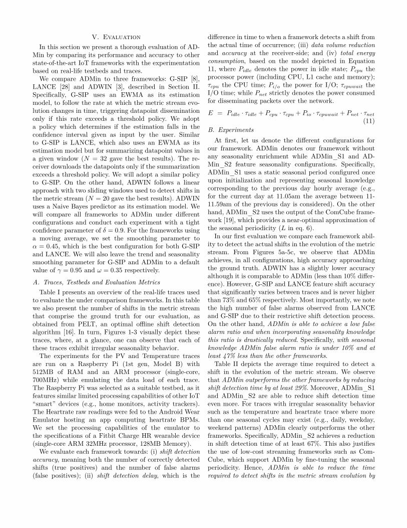
A. Traces, Testbeds and Evaluation MetricsTable I presents an overview of the real-life traces used

to evaluate the under comparison frameworks. In this tablewe also present the number of shifts in the metric streamthat comprise the ground truth for our evaluation, asobtained from PELT, an optimal offline shift detectionalgorithm [16]. In turn, Figures 1-3 visually depict thesetraces, where, at a glance, one can observe that each ofthese traces exhibit irregular seasonality behavior.

The experiments for the PV and Temperature tracesare run on a Raspberry Pi (1st gen, Model B) with512MB of RAM and an ARM processor (single-core,700MHz) while emulating the data load of each trace.The Raspberry Pi was selected as a suitable testbed, as itfeatures similar limited processing capabilities of other IoT“smart” devices (e.g., home monitors, activity trackers).The Heartrate raw readings were fed to the Android WearEmulator hosting an app computing heartrate BPMs.We set the processing capabilities of the emulator tothe specifications of a Fitbit Charge HR wearable device(single-core ARM 32MHz processor, 128MB Memory).

We evaluate each framework towards: (i) shift detectionaccuracy, meaning both the number of correctly detectedshifts (true positives) and the number of false alarms(false positives); (ii) shift detection delay, which is the

difference in time to when a framework detects a shift fromthe actual time of occurrence; (iii) data volume reductionand accuracy at the receiver-side; and (iv) total energyconsumption, based on the model depicted in Equation11, where Pidle denotes the power in idle state; Pcpu theprocessor power (including CPU, L1 cache and memory);τcpu the CPU time; Pi/o the power for I/O; τcpuwait theI/O time; while Pnet strictly denotes the power consumedfor disseminating packets over the network.

E = Pidle · τidle + Pcpu · τcpu + Pio · τcpuwait + Pnet · τnet

(11)B. Experiments

At first, let us denote the different configurations forour framework. ADMin denotes our framework withoutany seasonality enrichment while ADMin S1 and AD-Min S2 feature seasonality configurations. Specifically,ADMin S1 uses a static seasonal period configured onceupon initialization and representing seasonal knowledgecorresponding to the previous day hourly average (e.g.,for the current day at 11.05am the average between 11-11.59am of the previous day is considered). On the otherhand, ADMin S2 uses the output of the ComCube frame-work [19], which provides a near-optimal approximation ofthe seasonal periodicity (L in eq. 6).

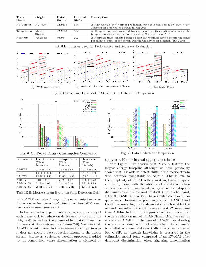
In our first evaluation we compare each framework abil-ity to detect the actual shifts in the evolution of the metricstream. From Figures 5a-5c, we observe that ADMinachieves, in all configurations, high accuracy approachingthe ground truth. ADWIN has a slightly lower accuracyalthough it is comparable to ADMin (less than 10% differ-ence). However, G-SIP and LANCE feature shift accuracythat significantly varies between traces and is never higherthan 73% and 65% respectively. Most importantly, we notethe high number of false alarms observed from LANCEand G-SIP due to their restrictive shift detection process.On the other hand, ADMin is able to achieve a low falsealarm ratio and when incorporating seasonality knowledgethis ratio is drastically reduced. Specifically, with seasonalknowledge ADMin false alarm ratio is under 10% and atleast 47% less than the other frameworks.

Table II depicts the average time required to detect ashift in the evolution of the metric stream. We observethat ADMin outperforms the other frameworks by reducingshift detection time by at least 29%. Moreover, ADMin S1and ADMin S2 are able to reduce shift detection timeeven more. For traces with irregular seasonality behaviorsuch as the temperature and heartrate trace where morethan one seasonal cycles may exist (e.g., daily, weekday,weekend patterns) ADMin clearly outperforms the otherframeworks. Specifically, ADMin S2 achieves a reductionin shift detection time of at least 67%. This also justifiesthe use of low-cost streaming frameworks such as Com-Cube, which support ADMin by fine-tuning the seasonalperiodicity. Hence, ADMin is able to reduce the timerequired to detect shifts in the metric stream evolution by

TraceName

Origin DataPoints

OptimalShifts

Description

PV Current PV Panel 1209598 194 A Photovoltaic (PV) current production trace collected from a PV panel every1 second for a period of 2 weeks in Jan 2015

Temperature MeteoStation

1209598 572 A Temperature trace collected from a remote weather station monitoring thetemperature every 1 second for a period of 2 weeks in Jan 2015

Heartrate Wearable 40908 202 A Heartrate trace collected from a Fitbit HR wearable device monitoring beatsper minute (bpm) of the person wearing the device for a month (Jun 2016)

TABLE I: Traces Used for Performance and Accuracy Evaluation

(a) PV Current Trace (b) Weather Station Temperature Trace (c) Heartrate Trace

Fig. 5: Correct and False Metric Stream Shift Detection Comparison

Fig. 6: On Device Energy Consumption ComparisonFramework PV Current

(TimeIntervals)

Temperature(TimeIntervals)

Heartrate(TimeIntervals)

ADWIN 9.34 ± 3.47 9.94 ± 3.84 10.39 ± 3.96G-SIP 10.02 ± 3.96 11.76 ± 4.16 14.17 ± 4.93LANCE 10.78 ± 4.12 12.63 ± 3.92 15.97 ± 4.12ADMin 6.04 ± 2.19 7.12 ± 1.97 8.03 ± 2.78ADMin S1 3.13 ± 2.03 5.11 ± 2.10 6.22 ± 2.83ADMin S2 2.62 ± 1.94 3.23 ± 2.26 4.73 ± 2.43

TABLE II: Metric Stream Evolution Shift Detection Delay

at least 29% and when incorporating seasonality knowledgeto the estimation model reduction is at least 67% whencompared to other frameworks.

In the next set of experiments we compare the ability ofeach framework to reduce on device energy consumption(Figure 6), as well as, the volume of IoT data and estima-tion error at the receiver-side (Figures 7-8). We note that,ADWIN is not present in the receiver-side comparison asit does not apply a data reduction scheme to the metricstream. Moreover, a reference baseline approach is addedto the comparison where dissemination is withhold by

Fig. 7: Data Reduction Comparison

applying a 10 time interval aggregation scheme.From Figure 6 we observe that ADWIN features the

largest energy footprint although we have previouslyshown that it is able to detect shifts in the metric streamwith accuracy comparable to ADMin. This is due tothe complexity of the ADWIN algorithm, linear in spaceand time, along with the absence of a data reductionscheme resulting in significant energy spent for datapointdissemination and the algorithm itself. On the other hand,LANCE, G-SIP and ADMin have similar complexity re-quirements. However, as previously shown, LANCE andG-SIP feature a high false alarm ratio which enables thenetwork controller of the IoT device at least x2 times morethan ADMin. In turn, from Figure 7 one can observe thatthe data reduction model of LANCE and G-SIP are not asefficient as ADMin. In the case of LANCE, downloadingthe entire window length of data when the summaryis labelled as meaningful drastically affects performance.For G-SIP, not enough knowledge is preserved in theestimation model (only comprised of an EWMA) afterdatapoint dissemination, often triggering dissemination

Fig. 8: Receiver-Side Mean Absolute Percentage Error

in subsequent intervals for model updating. Nonetheless,ADMin is able to reduce data volume by at least 71% whichaccounts for a reduction in energy consumption of at least83%. Most importantly, from Figure 8 one can observethat in regards to accuracy ADMin outperforms the otherframeworks by always maintaining accuracy at the receiverto at least 86%, increasing to at least 91% when seasonalitybehavior is acknowledged by the estimation model.

VI. ConclusionIn this paper we have presented ADMin, an adaptive

monitoring dissemination framework for IoT devices. Ourmain idea is to provide IoT devices with a lightweight andmodel-based framework capable of adapting the rate atwhich monitoring streams are disseminated to receivingentities based on the evolution, variability and seasonalityof the stream. The ADMin framework reduces IoT deviceenergy consumption, as well as, allocated bandwidth andthe volume of data disseminated through IoT networks.Exploiting the variability and seasonality of IoT moni-toring streams, ADMin incorporates novel low-cost andprobabilistic learning algorithms which efficiently modeland estimate at runtime the monitoring stream evolu-tion. Results show that ADMin is a viable solution thatis lightweight, practical and achieves a balance betweenefficiency and accuracy for numerous diverse and real data.Acknowledgement. This work is partially supported bythe EU Commission in terms of Unicorn 731846 H2020project (H2020-ICT-2016-1).

References[1] A. G. Barnett and A. J. Dobson, Introduction to Seasonality.

Berlin, Heidelberg: Springer Berlin Heidelberg, 2010, pp. 49–74.[2] H. Bauer, M. Patel, and J. Veira, “The internet of things: Sizing

up the opportunity,” McKinsey Report, Dec 2014.[3] A. Bifet and R. Gavalda, “Learning from time-changing data

with adaptive windowing,” in In SIAM International Confer-ence on Data Mining, 2010.

[4] K. M. Carter and W. W. Streilein, “Probabilistic reasoning forstreaming anomaly detection,” in Statistical Signal ProcessingWorkshop (SSP), 2012 IEEE. IEEE, 2012, pp. 377–380.

[5] Cisco, “Forecast and methodology 2014–2019,” Global CloudIndex, 2013.

[6] D. Trihinas, G. Pallis and M. D. Dikaiakos, “Monitoring Elas-tically Adaptive Multi-Cloud Services,” IEEE Transactions onCloud Computing, vol. 4, 2016.

[7] A. Deligiannakis, Y. Kotidis, and N. Roussopoulos, “Compress-ing historical information in sensor networks,” in Proceedings ofthe 2004 ACM SIGMOD International Conference on Manage-ment of Data, 2004, pp. 527–538.

[8] E. Gaura, J. Brusey, M. Allen, R. Wilkins, D. Goldsmith, andR. Rednic, “Edge Mining the Internet of Things,” SensorsJournal, IEEE, vol. 13, no. 10, pp. 3816–3825, Oct 2013.

[9] S. Gelper, R. Fried, and C. Croux, “Robust forecasting with ex-ponential and holt–winters smoothing,” Journal of forecasting,vol. 29, no. 3, pp. 285–300, 2010.

[10] C. C. Holt, “Forecasting seasonals and trends by exponentiallyweighted moving averages,” International journal of forecasting,vol. 20, no. 1, pp. 5–10, 2004.

[11] R. J. Hyndman and G. Athanasopoulos, “Forecasting: principlesand practice,” Online textbook, 2013.

[12] IDC, “Rich Data and the Increasing Value of IoT,” 2014.[13] W. Jiang, L. Shu, and D. W. Apley, “Adaptive cusum pro-

cedures with ewma-based shift estimators,” IIE Transactions,vol. 40, no. 10, pp. 992–1003, 2008.

[14] E. Keogh, K. Chakrabarti, M. Pazzani, and S. Mehrotra, “Lo-cally adaptive dimensionality reduction for indexing large timeseries databases,” SIGMOD, vol. 30, no. 2, pp. 151–162, 2001.

[15] S. Khalifa, M. Hassan, A. Seneviratne, and S. Das, “Energy-harvesting wearables for activity-aware services,” Internet Com-puting, IEEE, vol. 19, no. 5, pp. 8–16, Sept 2015.

[16] R. Killick, P. Fearnhead, and I. A. Eckley, “Optimal detectionof changepoints with a linear computational cost,” Journal ofthe American Statistical Association, vol. 107, no. 500, 2012.

[17] Y. Luo, Z. Li, and Z. Wang, “Adaptive cusum control chart withvariable sampling intervals,” Computational Statistics & DataAnalysis, vol. 53, no. 7, pp. 2693 – 2701, 2009.

[18] Y. Matsubara and Y. Sakurai, “Regime shifts in streams: Real-time forecasting of co-evolving time sequences,” in Proceedingsof the 22th ACM SIGKDD international conference on Knowl-edge discovery and data mining. ACM, 2016.

[19] Y. Matsubara, Y. Sakurai, and C. Faloutsos, “Non-linear miningof competing local activities,” in 25th Int’l Conference on WorldWide Web (WWW ’16), 2016, pp. 737–747.

[20] C. Perera, C. Liu, and S. Jayawardena, “The Emerging Internetof Things Marketplace From an Industrial Perspective: A Sur-vey,” Emerging Topics in Computing, IEEE Transactions on,vol. PP, no. 99, pp. 1–1, 2015.

[21] U. Raza, A. Camerra, A. L. Murphy, T. Palpanas, and G. P.Picco, “Practical data prediction for real-world wireless sensornetworks,” IEEE Transactions on Knowledge and Data Engi-neering, vol. 27, no. 8, pp. 2231–2244, Aug 2015.

[22] W. Shi and S. Dustdar, “The promise of edge computing,”Computer, vol. 49, no. 5, pp. 78–81, May 2016.

[23] A. Silberstein, R. Braynard, and J. Yang, “Constraint chaining:On energy-efficient continuous monitoring in sensor networks,”in Proceedings of the 2006 ACM SIGMOD International Con-ference on Management of Data, ser. SIGMOD ’06. New York,NY, USA: ACM, 2006, pp. 157–168.

[24] J. W. Taylor, “Exponential smoothing with a damped multi-plicative trend,” International Journal of Forecasting, vol. 19,no. 4, pp. 715 – 725, 2003.

[25] D. Trihinas, G. Pallis, and M. D. Dikaiakos, “AdaM: an Adap-tive Monitoring Framework for Sampling and Filtering on IoTDevices,” in IEEE International Conference on Big Data, 2015,pp. 717–726.

[26] D. Trihinas, G. Pallis, and M. Dikaiakos, “JCatascopia: Moni-toring Elastically Adaptive Applications in the Cloud,” in Clus-ter, Cloud and Grid Computing (CCGrid), 14th IEEE/ACMInternational Symposium on, May 2014, pp. 226–235.

[27] H.-L. Truong and S. Dustdar, “Principles for engineering iotcloud systems,” IEEE Cloud Computing, vol. 2, no. 2, 2015.

[28] G. Werner-Allen, S. Dawson-Haggerty, and M. Welsh, “Lance:optimizing high-resolution signal collection in wireless sensornetworks,” in Proceedings of the 6th ACM conference on Em-bedded network sensor systems. ACM, 2008, pp. 169–182.

[29] B. Zhang, N. Mor, J. Kolb, D. S. Chan, K. Lutz, E. Allman,J. Wawrzynek, E. Lee, and J. Kubiatowicz, “The cloud is notenough: Saving iot from the cloud,” in 7th USENIX Hot Topicsin Cloud Computing (HotCloud 15). USENIX, Jul. 2015.