Adjusted Plus-Minus for NHL Players usingRidge Regression with Goals, Shots, Fenwick,

and Corsi

Brian Macdonald∗

October 3, 2012

Abstract

Regression-based adjusted plus-minus statistics were developed in bas-ketball and have recently come to hockey. The purpose of these statistics isto provide an estimate of each player’s contribution to his team, independentof the strength of his teammates, the strength of his opponents, and othervariables that are out of his control. One of the main downsides of the or-dinary least squares regression models is that the estimates have large errorbounds. Since certain pairs of teammates play together frequently, collinear-ity is present in the data and is one reason for the large errors. In hockey, therelative lack of scoring compared to basketball is another reason. To dealwith these issues, we use ridge regression, a method that is commonly usedin lieu of ordinary least squares regression when collinearity is present inthe data. We also create models that use not only goals, but also shots, Fen-wick rating (shots plus missed shots), and Corsi rating (shots, missed shots,and blocked shots). One benefit of using these statistics is that there areroughly ten times as many shots as goals, so there is much more data whenusing these statistics and the resulting estimates have smaller error bounds.The results of our ridge regression models are estimates of the offensive anddefensive contributions of forwards and defensemen during even strength,power play, and short handed situations, in terms of goals per 60 minutes.The estimates are independent of strength of teammates, strength of oppo-nents, and the zone in which a player’s shift begins.

Keywords: adjusted plus-minus, plus-minus, hockey, nhl, performance analysis

∗email: bmac@jhu.edu

1

arX

iv:1

201.

0317

v2 [

stat

.AP]

1 O

ct 2

012

Contents1 Introduction 3

1.1 Brief summary of the new models . . . . . . . . . . . . . . . . . 41.2 Notation . . . . . . . . . . . . . . . . . . . . . . . . . . . . . . . 51.3 Example of the results . . . . . . . . . . . . . . . . . . . . . . . 6

2 Ridge Regression Model 82.1 Differences in OLS and Ridge Estimates . . . . . . . . . . . . . . 102.2 Year-to-year correlations . . . . . . . . . . . . . . . . . . . . . . 11

3 Results 123.1 Four-year Selke Trophy finalists for Best Defensive Forward . . . 133.2 Four-year Norris Trophy finalists for Best Defensemen . . . . . . 143.3 Four-year Hart Trophy finalists for Most Valuable Player . . . . . 15

4 Conclusions and Future Work 15

5 Appendix 195.1 Ordinary Least Squares . . . . . . . . . . . . . . . . . . . . . . . 195.2 Ridge Regression . . . . . . . . . . . . . . . . . . . . . . . . . . 205.3 Choosing λ . . . . . . . . . . . . . . . . . . . . . . . . . . . . . 215.4 Supplemental figures . . . . . . . . . . . . . . . . . . . . . . . . 23

List of Tables1 Summary of notation for APM results using goals. . . . . . . . . . 62 The top 10 offensive players in the NHL according to Goff. . . . . 73 Sidney Crosby’s APM statistics during 2007-11 using goals. . . . 74 Alex Ovechkin’s EV offense statistics, with standard errors. . . . . 85 The top 5 defensive forwards according to Gdef. . . . . . . . . . . 136 The top 5 defensemen during the last 4 seasons, according to G. . 147 The top 5 players according to G. . . . . . . . . . . . . . . . . . . 15

List of Figures1 Estimates of Goff

PP,60 for some players, for different values of λ . . . 112 Goff

PP,60 vs λ for players whose estimates change the most . . . . . 123 Year-to-year correlations of OLS and Ridge estimates . . . . . . . 134 Shift lengths for all PP shifts and PP shifts when a goal is scored . 235 Distribution of players’ ice time for EV and PP situations . . . . . 24

2

1 IntroductionThough the plus-minus statistic was first used in hockey, advanced versions ofplus-minus have been developing more quickly in basketball. These new versionsattempt to correct one or more of the problems associated with the traditional plus-minus statistic, which depends heavily on the strength of a player’s teammatesand opponents, and on other variables out of a player’s control. Regression-basedversions of adjusted plus-minus (APM) statistics for NBA players can be foundin Winston (2009), Rosenbaum (2004), Lewin (2007), Witus (2008), Ilardi andBarzilai (2008), Sill (2010), and Fearnhead and Taylor (2011).

In Macdonald (2011a) and Macdonald (2011b), the author developed similarmodels for hockey. In Macdonald (2011a), the author used weighted least squaresmodels similar to those in Rosenbaum (2004) and Ilardi and Barzilai (2008) tofind the estimates of each player’s offensive and defensive contribution duringeven strength situations, adjusted for the strength of his teammates and opponents.The contributions are given in terms of goals per 60 minutes and goals per season.Special teams situations are addressed in Macdonald (2011b). Information aboutthe zone in which each shift begins was also used in Macdonald (2011b) in orderto get estimates that are independent of the zone on the ice in which a playertypically begins his shifts.

In many of the basketball articles, and also in the hockey articles Macdonald(2011a) and Macdonald (2011b), it was noted that one downside of the ordinaryleast squares regression models is that the results can have large error bounds,which are measures of uncertainty in the estimates. Since two main uses of theseestimates could be (1) deciding which players to trade for and (2) establishing pa-rameters for salary negotiations, smaller errors, and hence more precise estimates,have significant value to NHL analysts and decision-makers.

One reason for the large errors is the high collinearity in the data caused byteammates who play together frequently, a common occurrence in many sports.For example, Henrik and Daniel Sedin, twin brothers who play for the VancouverCanucks, are almost always on the ice together. A regression model will havea difficult time telling them apart (both statistically and biologically) and theirestimates tend to have large errors. In an extreme case where two players alwaysplay together, the ordinary least squares estimates will not even be unique.

Another reason for the high errors in hockey is the relative lack of scoringwhen compared to a sport like basketball. A typical hockey team only scores twoto four goals per game on average during a season. The low goal scoring rates,coupled with randomness and luck involved with goal scoring, makes it difficultto properly judge players using goals alone without using multiple seasons ofdata. Additionally, a player’s goals for and goals against while he is on the iceis dependent on the quality of goalies on the ice. Ideally, one would prefer toestimate a player’s abilities in a way that is independent of the quality of the

3

goalies he faces, and independent of the quality of goalies on his team.

1.1 Brief summary of the new modelsIn light of these observations, we make two modifications to the models givenin Macdonald (2011a) and Macdonald (2011b). First, in lieu of ordinary leastsquares regression models, we use ridge regression models (Hoerl (1962), Hoerland Kennard (1970)), similar to the model used for basketball in Sill (2010). Ridgeregression frequently reduces the error bounds in the estimates and improves thepredictive performance of the model when collinearly exists in the data. Ridge re-gression introduces bias in the estimates, but the tradeoff is typically worthwhile.The model is discussed in detail in Section 2.

The second change we make is to form additional models that use three otherstatistics, in addition to goals, as the dependent variable. These additional mod-els use shots, Fenwick rating (shots plus missed shots), and Corsi rating (shots,missed shots, and blocked shots). These statistics were chosen because each ofthem has been shown to be very good indicators of performance at the team level(JLikens (2011), Ferrari (2009)).

There are pros and cons to using these statistics, and that is one reason thatwe will use them in addition to goals and not instead of goals. For example,on one hand, shots, Fenwick rating, and Corsi rating ignore the shooting abilityof players, although many hockey analysts would argue that a player’s shootingability is not nearly as significant as his ability to generate shots. Also, somewould argue that missed shots and blocked shots should not be included or shouldnot be considered good, since they are attempted shots that never reached thegoal. However, if a team has more shots, missed shots, and blocked shots thantheir opponents, it is most likely an indication of a territorial advantage and anadvantage in terms of puck possession. In order to take a shot, a player mustpossess the puck, and typically that player is also in the offensive zone.

The relationships among goals, shots, Fenwick rating, and Corsi rating aredescribed well in JLikens (2011) and discussed further in Macdonald (2012). Inboth articles, the authors show that shots, Fenwick rating, and Corsi rating arebetter indicators than goals of a team’s future performance when one uses datafrom only half of a season. Based on this analysis, we believe the results based onshots, Fenwick rating and Corsi rating do have value, especially for our modelsthat are based on only one season’s worth of data. The reader can decide for him-or herself how much value those results have.

One nice benefit of using of these additional statistics is that they are far moreprevalent than goals. Typically, there are roughly 10 shots to every goal. The ex-tra data goes a long way to producing estimates with much smaller error bounds.Also, for the most part, those statistics are independent of goalies, so the strengthof the goalies on a player’s team will not have much of an affect on the estimates

4

of his contributions. When using goals, the estimate of a player’s defensive con-tribution, in particular, can be positively or negatively affected by the performanceof the goalie playing behind him.

In order to more easily compare the results based on these additional statis-tics with the results based on goals, the new results were rescaled using leagueaverage shooting percentages. By shooting percentages we mean goals per shot(Goals

Shots

), goals per Fenwick rating

( GoalsShots+Missed Shots

), and goals per Corsi rating( Goals

Shots+Missed Shots+Blocked Shots

). League averages of these shooting percentages

were computed for even strength, power play, and short handed situations sepa-rately, using data from the last four full NHL seasons.

The results based on shots, Fenwick rating, and Corsi rating were then rescaledby multiplying by the league average goals per shot, goals per Fenwick rating, andgoals per Corsi rating, respectively. These results are in the units of expected goalsper 60 minutes based on shots, Fenwick, or Corsi. A player’s rescaled resultsbased on shots can be thought of as his contribution to his team, in the units ofexpected goals per 60 minutes, based on shots for and shots against when he wason the ice. The results remain independent of the strength of his teammates, thestrength of his opponents, and the zone in which his shifts begin. The rescaledresults based on Fenwick rating and Corsi rating can be interpreted similarly.

We use four separate ridge regression models for even strength situations usingeach of these four statistics (goals, shots, Fenwick rating, and Corsi rating) as theresponse variable. Each even strength model gives an even strength offensive anddefensive component of APM for each player in terms of goals per 60 minutes orexpected goals per 60 minutes. These components can be added to give a player’stotal contribution at even strength in terms of goals per 60 minutes. We alsohave four separate models for special teams situations, one for each of the fourstatistics. Each special teams model gives an offensive and defensive componenton the power play, as well as an offensive and defensive component during shorthanded situations, in terms of goals per 60 minutes. In total, we get 36 estimatesfor each player in terms of goals per 60 minutes. If the results are expressed interms of goals per season, then even strength, power play, and shorthanded resultscan be added to give estimates of offensive, defensive, and total contributions inall situations, in terms of goals per season. So, in this case, we get 48 differentratings for each player. This can be a bit of information overload, and when wepresent the results here, we will need to be selective regarding which componentsof APM are listed. Notation will be important as well.

1.2 NotationNotation for the offensive, defensive, and total contribution of a player (forward ordefensemen) during even strength, power play, and short handed situations, using

5

the model with goals as the response variable, is given in Table 1. The adjusted

Table 1: Summary of notation for APM results using goals. For each player (for-ward or defensemen), we have offensive, defensive, and total contributions duringeven strength, power play, and short handed situations, in terms of goals per sea-son.

Strength Offense Defense Total

Even strength GoffEV Gdef

EV GEV

Power play GoffPP Gdef

PP GPP

Short handed GoffSH Gdef

SH GSH

All situations Goff Gdef G

plus-minus results based on shots, Fenwick rating and Corsi rating are denotedsimilarly, except with “S”, “F”, and “C”, respectively, instead of the “G” that isused for goals. For example, the even strength offensive component of APM us-ing goals, shots, Fenwick rating, and Corsi rating are denoted Goff

EV ,SoffEV ,F

offEV and

CoffEV , respectively. The per 60 minute versions of these statistics are denoted simi-

larly, but with a subscript of “60” included. For example, even strength offensivecomponent of adjusted plus-minus per 60 minutes using goals is denoted Goff

EV,60.

1.3 Example of the resultsIn Table 2, we give an example of the results. We list the top 10 players in offenseduring the 2007-08, 2008-09, 2009-10, and 2010-11 seasons according to Goff,the offensive component of APM in terms of goals per season. We also list theplayers’ offensive contributions according to the APM models based on the otherstatistics.

Recall that Soff, Foff, and Coff have been rescaled by multiplying by the leagueaverage goals per shot, goals per Fenwick rating, and goals per Corsi rating, re-spectively. Note that these statistics are in the units of goals per season or expectedgoals per season based on shots, Fenwick, or Corsi, so they do depend on playingtime. Sidney Crosby, for example, has missed significant time in two of the fourseasons, and that has a big impact on his rating, although he still leads the leaguein Goff by a sizeable margin.

Some per 60 minute results, GoffEV,60 and Soff

EV,60, along with their standard er-rors, are given in the last four columns of that table. These statistics are indepen-dent of playing time, so they do not depend on how much their coaches play them.They also do not depend on how much time these players have spent on injured

6

Table 2: The top 10 offensive players in the NHL according to Goff.

Player Pos Team Goff Soff Foff Coff GoffEV,60 Err Soff

EV,60 Err

1 Sidney Crosby C PIT 23 12 13 14 0.83 0.20 0.42 0.072 Jonathan Toews C CHI 18 8 8 9 0.45 0.20 0.22 0.073 Alex Ovechkin LW WSH 17 17 20 24 0.46 0.18 0.45 0.074 Daniel Sedin LW VAN 16 13 13 15 0.47 0.18 0.44 0.085 Joe Thornton C S.J 16 11 11 15 0.34 0.18 0.26 0.066 Nicklas Backstrom C WSH 16 11 12 14 0.23 0.19 0.28 0.077 Evgeni Malkin C PIT 15 11 11 12 0.40 0.20 0.31 0.068 Ryan Getzlaf C ANA 15 6 8 9 0.31 0.19 0.07 0.079 Pavel Datsyuk C DET 15 10 11 12 0.53 0.19 0.27 0.07

10 Jason Spezza C OTT 13 7 8 9 0.37 0.21 0.25 0.07

reserve. We believe that both the per season and per 60 minutes versions of thesestatistics have value, and we will continue to list both versions in our tables.

In this paper, we will mostly give results based on models that contain datafrom four NHL seasons: 2007-08, 2008-09, 2009-10, and 2010-11. However,since we are now using ridge regression, single season results are stable enough tohave value. One might prefer to see a player’s progression from season to seasonrather than seeing a single number for all four years. Also, one might prefer tomake adjustments so that the statistics for a player are relative to a replacementplayer at the same position. An example of Sidney Crosby’s APM statistics in eachof the past four seasons, with adjustments for position and replacement players, isgiven in Table 3. We have also included his 4-year results for comparison.

Table 3: Sidney Crosby’s APM statistics over the past four seasons using goals.

Year Age GP Goff Gdef G GoffEV Gdef

EV GEV GoffPP Gdef

PP GPP

2007 20 53 25 9 33 19 7 26 6 2 72008 21 77 30 3 33 21 2 23 9 1 102009 22 81 37 4 41 31 2 34 5 2 72010 23 41 17 1 18 13 0 13 3 1 54-yr 20-23 63 29 1 30 23 1 24 5 1 6

We also note that the errors in our estimates are lower than those reported inMacdonald (2011a) and Macdonald (2011b), where the author used ordinary leastsquares (OLS) regression instead of ridge regression. As an example, we giveAlex Ovechkin’s even strength offensive contributions per 60 minutes in Table 4,along with their standard errors. The errors in Ovechkin’s Goff

EV,60 are smaller thanthose reported in Macdonald (2011a) and Macdonald (2011b). Also, the errors in

7

Ovechkin’s SoffEV,60, Foff

EV,60, and CoffEV,60 are smaller than the errors in Goff

EV,60. Thistrend can also be seen in Table 2. The standard errors in Soff

EV,60 are much lowerthan the standard errors in Goff

EV,60 for all of the players in that table. The errors arestill not small enough to be ignored, as the confidence intervals of many of the es-timates still overlap. Nevertheless, the APM estimates with smaller error bounds,coupled with the additional APM estimates based on shots, Fenwick rating, andCorsi rating, are useful metrics with which to analyze the performance of NHLplayers.

Table 4: Alex Ovechkin’s EV offense statistics, with standard errors.

Player Pos Team GoffEV,60 Err Soff

EV,60 Err FoffEV,60 Err Coff

EV,60 Err

Alex Ovechkin LW WSH 0.46 0.18 0.45 0.07 0.53 0.06 0.63 0.05

The rest of this paper is organized as follows. First, we describe the ridgeregression models in detail in Section 2. In Section 3, we give the players thatAPM determines as the Hart Trophy, Norris Trophy, and Selke Trophy finalists(most valuable player, best defensemen, and best defensive forward, respectively)during the 2007-08, 2008-09, 2009-10, and 2010-11 seasons combined. We finishwith conclusions and future work in Section 4. In the Appendix, we give a briefcomparison of ordinary least squares and ridge regression, and describe how wechose our ridge parameter in our ridge regression models.

2 Ridge Regression ModelWe now describe the setup of our model. We use information about the playerson the ice during every shift of every game during the 2007-08, 2008-09, 2009-10, and 2010-11 seasons, as well as the outcome of each shift. We divide thisdata into even strength and special teams situations, and we remove empty netsituations from both data sets. Each shift gives two lines of data: one line cor-responding to the goals per 60 minutes scored by the home team, and one linecorresponding to the goals per 60 minutes scored by the away team. Both of theseobservations are weighted by the duration of that shift. We denote the total num-ber of observations by N. For even strength, we have N = 2,324,528, while forspecial teams situations, we have N = 461,022. We note that the average durationof a shift is 4.5 seconds longer for special teams than for even strength. Other ob-servations about shift lengths and ice time for players, along with accompanyingfigures, can be found in Figures 4 and 5 the Appendix.

Let J denote the number of players in the league, let y denote the goals (orshots, Fenwick rating, or Corsi rating) per 60 minutes during an observation, and

8

let X j and D j be indicator variables that are defined as follows:

X j =

1, skater j is on offense during the observation;0, skater j is not playing or is on defense during the observation;

D j =

1, skater j is on defense during the observation;0, skater j is not playing or is on offense during the observation;

(1)

where 1 ≤ j ≤ J. Note that by “skater” we mean a forward or a defensemen,but not a goalie. We also note that for the models which use goals, we includeddefensive variables for goalies. Let Zo f f and Zde f be indicator variables definedas follows:

Zo f f =

1, the observation corresponds to a shift that begins with a faceoff in

the offensive zone,0, otherwise

Zde f =

1, the observation corresponds to a shift that begins with a faceoff in

the defensive zone,0, otherwise

(2)

To clarify, we give an example. Suppose that in one shift, skaters 1-5 are onthe ice for the home team, and skaters 6-10 are on the ice for the away team.Suppose that this is a shift of duration t1 seconds, and that the home team scores agoal during this shift. For this shift we would have two lines of data, one for goalsper 60 minutes scored by the home team, and the second for goals per 60 minutesscored by the away team. These two rows of data would look like this:

X = [1 1 1 1 1 0 0 0 0 0 0 · · ·0],D = [0 0 0 0 0 1 1 1 1 1 0 · · ·0], y =1t1·3600,

X = [0 0 0 0 0 1 1 1 1 1 0 · · ·0],D = [1 1 1 1 1 0 0 0 0 0 0 · · ·0], y =0t1·3600.

We note that 1t1

is in the units of goals per second, so we multiple by 3,600 to getgoals per 60 minutes. For even strength situations, we start with the followinglinear model:

y = β0 +β1X1 + · · ·+βJXJ +δ1D1 + · · ·+δJDJ +ζo f f Zo f f +ζde f Zde f . (3)

The quantities of interest are the β js and δ js, which are player j’s offensive anddefensive contributions, respectively, in terms of goals per 60 minutes. The coef-ficients ζo f f and ζde f can be regarded as estimates of the value of starting a shiftin the offensive or defensive zone, respectively, in terms of goals per 60 minutes.

9

For special teams situations, we start with a model that is similar to (3) and isdescribed in Macdonald (2011b). In total, there are 8 models: an even strengthmodel and a special teams model for each of the four statistics.

A linear model like (3) can also be expressed as a system of linear equationsin matrix form as

y = Xβ , (4)

where y is an N × 1 vector of response variables, X is an N × (2J + 3) matrixof the explanatory variables, and β is an (2J + 3)× 1 vector of coefficients, thequantities we are interested in. Typically, when the number of observations, N, ismuch greater than the number of explanatory variables, 2J +3, no solution to (4)exists, and one must find some sort of “best fit” solution.

Instead of using OLS as in Macdonald (2011a) and Macdonald (2011b) tofind the best fit, we use ridge regression. For the sake of those readers who areunfamiliar with ridge regression, we give a brief description of how to find the bestfit estimates using OLS regression and ridge regression, and how the two methodsare related, in the Appendix. We also discuss how we chose the ridge parameterλ in that section.

2.1 Differences in OLS and Ridge EstimatesThe effect that this ridge parameter λ has on the estimates can be seen in Figure1. In this example, we plot the estimated coefficient for Goff

PP,60 (offensive contri-bution on the power play in terms of goals per 60 minutes) of a few players inthe league for different choices of λ . Note that when λ = 0, Pavel Datsyuk (solidred line) actually has a negative estimate, and Brandon Dubinsky (solid blue line)has a very high positive estimate in line with the league’s elite offensive players.Dubinsky is a valuable offensive player, but one would not expect his rating tobe that much higher than Datsyuk’s rating or among the league’s elite. Also, wewould not consider Datsyuk to be a below average player on the power play. Wenote that λ = 0 corresponds to the ordinary least squares estimates, so these arethe estimates we would have gotten for Dubinsky and Datsyuk if we had not usedridge regression.

However, notice that for larger choices of λ , the estimates begin to stabi-lize. Datsyuk’s estimate moves towards the estimates of the league’s elite players,while Dubinsky’s estimate returns to a more reasonable level. These estimatesagree with most people’s intuition that Datysuk is an elite offensive player, whileDubinsky is an above average offensive player, but not an elite player as his ordi-nary least squares estimate suggested.

For Dubinsky, the unexpected result for λ = 0 is probably due to minimalplaying time. For Datsyuk, it is probably due to the fact that he spent 90% of his

10

0.0 0.5 1.0 1.5 2.0

0.0

0.5

1.0

1.5

2.0

2.5

Estimates of GPPoff vs λ

λ

Est

imat

e of

GP

Pof

f

Pavel Datsyuk CSidney Crosby CAlex Ovechkin LWHenrik Sedin CDaniel Sedin LWNicklas Lidstrom DBrandon Dubinsky C

Datsyuk's OLS estimate

Dubinsky's OLS estimate

Datsyuk's ridge estimate

Dubinsky's ridge estimate

Figure 1: Estimates of GoffPP,60 for some players, for different values of λ .

power play time with one of his teammates, Nicklas Lidstrom. While Datsyuk’sestimate starts below zero for λ = 0 and increases as λ increases, Lidstrom’sestimate (dotted and dashed, light blue line) is off the figure near 4.0 for λ = 0,and rapidly decreases as λ increases. While we would expect Lidstrom to havea good offensive rating on the power play, 4.0 is unusually high, and the ridgeregression seems to be tempering Lidstrom’s estimate while correcting Datsyuk’s.

Datsyuk and Dubinsky are not the only players whose estimates exhibit thisbehavior. We give the tracecurves of the 25 players whose coefficients were themost positively (resp. negatively) affected by the ridge regression as the dotted(resp. solid) lines in Figure 2. In many cases, there are drastic changes in aplayer’s value relative the other players in the league. A player may be worth 1goal per 60 minutes more than another player according to their OLS estimates(λ = 0) but worth 0.5 goals per 60 minutes less according to their ridge estimates(λ = 0.5).

2.2 Year-to-year correlationsWe note that the ridge estimates tend to be more consistent from year to year thanthe OLS estimates. In Figure 3 we give three examples of year-to-year corre-lations for three of the components of APM. In the left figure, we see that ourridge estimates for offense at even strength using goals tend to be more consistent

11

0.0 0.1 0.2 0.3 0.4 0.5

−2

02

4

Estimates of GPPoff vs λ

λ

Est

imat

e of

GP

Pof

f

RisersFallers1st percentile99th percentile

Figure 2: Estimates of GoffPP,60 for different values of λ for the 25 players whose

coefficients were the most positively (resp. negatively) affected by the ridge re-gression, plotted as dashed (resp. solid) lines.

than the corresponding OLS estimates from Macdonald (2011a) (which also usedgoals). Also, the ridge estimates that use shots, Fenwick, and Corsi tend to bemore consistent than the ridge estimates that use goals.

In the middle figure, we see that these trends are true for power play offenseas well. For short handed defense, the ridge estimates using goals are not moreconsistent than the OLS estimates, although the correlations for shots, Fenwickand Corsi are still higher. We note that, in general, the even strength estimatestend to have higher year-to-year correlations than the power play and short handedestimates. This trend is expected, since there is much less data for special teamssituations than for even strength situations.

3 ResultsWe now consider performance during the 2007-08, 2008-09, 2009-10, and 2010-11 seasons combined and determine the “four-year” Selke Trophy finalists (bestdefensive forwards), Norris Trophy finalists (best defensemen), and Hart Trophyfinalists (most valuable players), according to APM. Although the NHL typicallyannounces three finalists for each trophy, we will give our top 5 finalists for each

12

OLS Goals Shots Fenwick Corsi

Year−to−year correlations of APM estimates (EV offense)

Cor

rela

tion

0.0

0.2

0.4

0.6

0.28

0.36

0.47

0.56

0.63

OLS Goals Shots Fenwick Corsi

Year−to−year correlations of APM estimates (PP offense)

Cor

rela

tion

0.0

0.2

0.4

0.6

0.18

0.26

0.340.39

0.44

OLS Goals Shots Fenwick Corsi

Year−to−year correlations of APM estimates (SH defense)

Cor

rela

tion

0.0

0.2

0.4

0.6

0.22 0.210.26

0.29 0.3

Figure 3: A comparison of year-to-year correlations for OLS estimates (OLS)and our new ridge regression estimates (Goals, Shots, Fwick, Corsi). (Left) Evenstrength offense, minimum 500 minutes. (Middle) Power play offense, minimum150 minutes. (Right) Short handed defense, minimum 150 minutes. To computethe correlations, the per 60 minutes versions of these statistics were used.

award and discuss other notable players.

3.1 Four-year Selke Trophy finalists for Best Defensive For-ward

Each season, the Selke Trophy is awarded to the forward that “best excels at thedefensive aspects of the game” NHL.com (2010). In practice, the award winner istypically a great defensive forward who contributes offensively as well. In Table5, we give the top defensive forwards in the league during the 2007-08, 2008-09, 2009-10, and 2010-11 seasons according to Gdef. Recall that Soff, Foff, Coff

Table 5: The top 5 defensive forwards according to Gdef.

Player Pos Team Gdef Sdef Fdef Cdef GdefEV,60 Err Sdef

EV,60 Err

Pavel Datsyuk C DET 12 8 7 6 0.44 0.19 0.30 0.07David Krejci C BOS 11 3 2 0 0.52 0.20 0.18 0.07Chris Higgins LW VAN 10 0 −1 −2 0.33 0.21 0.03 0.07Tomas Plekanec C MTL 10 −0 −1 −3 0.30 0.20 0.03 0.07Mikko Koivu C MIN 9 3 3 3 0.53 0.21 0.20 0.08

have been rescaled by multiplying by the league average goals per shot, goals perFenwick rating, and goals per Corsi rating, respectively. Recall that these statisticsare in the units of goals per season or expected goals per season based on shots,Fenwick, or Corsi.

Pavel Datsyuk seems to be the clear choice as the best defensive forward inthe NHL according to APM. He is the league leader in all 4 flavors of defensive

13

contribution, and is also the best offensive player on the list. The voters seem toagree: Datsyuk was awarded the Selke Trophy in 2007-08, 2008-09, and 2009-10, and he was a finalist in 2010-11. Tomas Plekanec and Chris Higgins areon this list, but one might consider the next best candidates to be David Krejicand Mikko Koivu due to their superior ability to reduce the opposition’s shots,Fenwick rating and Corsi rating. Interestingly, multi-year finalist and 2010-11winner Ryan Kesler is not on this list, although he did have very good numbers in2010-11. We note that 5 other players were tied with Koivu for 5th in Gdef with9 to round out the top 10 in that category. Daymond Langkow, who was 11th inGdef with 8, missed the top 10 in Gdef, but was second in Sdef, and third in bothFdef and Cdef. In light of those rankings, Langkow could be considered one of thebest defensive forwards in the game.

3.2 Four-year Norris Trophy finalists for Best DefensemenThe James Norris Memorial Trophy is given each year to the defensemen who“demonstrates throughout the season the greatest all-round ability in the position”NHL.com (2010). In Table 6, we give the top defensemen in the league duringthe 2007-08, 2008-09, 2009-10, and 2010-11 seasons according to G. It is not too

Table 6: The top 5 defensemen during the last 4 seasons, according to G.

Player Pos Team G S F C GoffEV,60 Soff

EV,60 GoffPP,60 Err Soff

PP,60 Err

Zdeno Chara D BOS 19 9 9 10 0.10 0.21 0.43 0.33 0.58 0.07Nicklas Lidstrom D DET 19 1 3 5 −0.06 0.07 1.37 0.26 0.71 0.05Brian Campbell D CHI 14 7 7 8 0.12 0.16 0.23 0.36 0.32 0.08Andrei Markov D MTL 13 −3 −1 1 0.20 0.13 1.75 0.37 0.59 0.08Brian Rafalski D DET 13 9 8 11 −0.02 0.22 0.84 0.30 0.65 0.06

surprising that Zdeno Chara and Nicklas Lidstrom were the best defenseman inthe NHL during those seasons according to G. Zdeno Chara’s APM results basedon shots, Fenwick rating, and Corsi rating are better than those of Lidstrom, soone might choose to select him as the best defenseman. Brian Campbell andBrian Rafalski are both strong across the board. Interestingly, Andrei Markovdoes not rate very well in the APM estimates based on shots, Fenwick rating,and Corsi rating. One might prefer to include Chris Pronger, Dan Boyle, or KrisLetang instead of Markov on this list due to their ratings in S,F and C. Boyle, forexample, led the league in S, F and C.

14

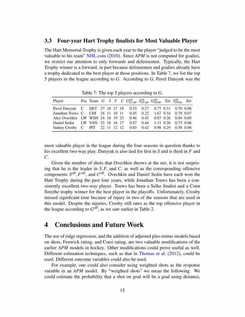
3.3 Four-year Hart Trophy finalists for Most Valuable PlayerThe Hart Memorial Trophy is given each year to the player “judged to be the mostvaluable to his team” NHL.com (2010). Since APM is not computed for goalies,we restrict our attention to only forwards and defensemen. Typically, the HartTrophy winner is a forward, in part because defensemen and goalies already havea trophy dedicated to the best player at those positions. In Table 7, we list the top5 players in the league according to G. According to G, Pavel Datsyuk was the

Table 7: The top 5 players according to G.

Player Pos Team G S F C GoffEV,60 Soff

EV,60 GoffPP,60 Err Soff

PP,60 Err

Pavel Datsyuk C DET 27 18 17 18 0.53 0.27 0.77 0.31 0.70 0.06Jonathan Toews C CHI 24 11 10 11 0.45 0.22 1.67 0.34 0.79 0.07Alex Ovechkin LW WSH 24 18 19 23 0.46 0.45 0.87 0.26 0.84 0.05Daniel Sedin LW VAN 23 16 16 17 0.47 0.44 1.11 0.26 0.73 0.06Sidney Crosby C PIT 22 11 12 12 0.83 0.42 0.98 0.29 0.58 0.06

most valuable player in the league during the four seasons in question thanks tohis excellent two-way play. Datsyuk is also tied for first in S and is third in F andC.

Given the number of shots that Ovechkin throws at the net, it is not surpris-ing that he is the leader in S,F, and C, as well as the corresponding offensivecomponents Soff,Foff, and Coff. Ovechkin and Daniel Sedin have each won theHart Trophy during the past four years, while Jonathan Toews has been a con-sistently excellent two-way player. Toews has been a Selke finalist and a ConnSmythe trophy winner for the best player in the playoffs. Unfortunately, Crosbymissed significant time because of injury in two of the seasons that are used inthis model. Despite the injuries, Crosby still rates as the top offensive player inthe league according to Goff, as we saw earlier in Table 2.

4 Conclusions and Future WorkThe use of ridge regression, and the addition of adjusted plus-minus models basedon shots, Fenwick rating, and Corsi rating, are two valuable modifications of theearlier APM models in hockey. Other modifications could prove useful as well.Different estimation techniques, such as that in Thomas et al. (2012), could beused. Different outcome variables could also be used.

For example, one could also consider using weighted shots as the responsevariable in an APM model. By “weighted shots” we mean the following. Wecould estimate the probability that a shot on goal will be a goal using distance,

15

type of shot, and other details as explanatory variables. Such shot quality modelshave been developed by Ken Krzywicki in Krzywicki (2005), Krzywicki (2009),and Krzywicki (2010) and Michael Schuckers in Schuckers (2011). Then, eachshot can be weighted based on the probability that it will be a goal. In a forth-coming article Macdonald et al., the authors create a shot quality model similarto Krzywicki’s logistic regression models, and use the resulting weighted shots asthe outcome variable in a ridge regression model similar to the one described inthis paper. The results of this model are estimates of W , an adjusted plus-minusrating based on weighted shots.

Also, recall that Fenwick rating and Corsi rating are combinations of shots,missed shots, and blocked shots, and are a good indication of possession advan-tage and team performance in general. One could build on the idea of using thosestatistics and consider other statistics like hits, faceoffs, and zone starts as well.In Macdonald (2012), the author estimates the combinations of these statistics arethe best predictors of goal scoring at the team level. The results of the modelcan be interpreted as “expected goals”. These expected goals are then used as theoutcome in a ridge regression similar to the model described in this paper. Theresults are estimates of E, an adjusted plus-minus rating based on expected goals.Another approach that uses several different statistics can be found in Schuckerset al. (2011).

We hope that the ideas presented in this paper will be useful to fans, analysts,coaches and teams as they analyze the performance of NHL players, and willinspire future work in performance analysis in hockey.

AcknowledgementsI would like to thank William Pulleyblank for many useful conversations aboutthis work and for his comments and suggestions after reading a draft of the paper.I would also like to thank the referees for many comments and suggestions thatimproved the quality of this paper.

ReferencesBretscher, O. (2009): Linear Algebra with Applications, Pearson Prentice Hall,

4th edition.

Fearnhead, P. and B. M. Taylor (2011): “On estimating the abilityof nba players,” Journal of Quantitative Analysis in Sports, 7,11, URL http://EconPapers.repec.org/RePEc:bpj:jqsprt:v:7:

y:2011:i:3:n:11.

16

Ferrari, V. (2009): “Possession is Everything,” http://vhockey.blogspot.

com/2009/05/possession-is-everything.html, Accessed 09-16-2011.

Girard, D. (1991): “Asymptotic optimality of the fast randomized versions ofGCV and CL in ridge regression and regularization,” Ann. Statist., 19,1950–1963.

Hoerl, A. E. (1962): “Application of ridge analysis to regression prob-lems,” Chemical Engineering Progress, 58, 54?59, URL http:

//scholar.google.com/scholar?hl=en&btnG=Search&q=intitle:

Application+of+ridge+analysis+to+regresion+problems#0.

Hoerl, A. E., R. W. Kannard, and K. F. Baldwin (1975): “Ridge regression:somesimulations,” Communications in Statistics, 4, 105–123, URL http://

www.tandfonline.com/doi/abs/10.1080/03610927508827232.

Hoerl, A. E. and R. W. Kennard (1970): “Ridge regression: Biased estimation fornonorthogonal problems,” Technometrics, 12, 55–67.

Hutchinson, M. (1989): “A stochastic estimator of the trace of the influence matrixfor Laplacian smoothing splines,” Commun. Stat. Simula., 18, 1059–1076.

Ilardi, S. and A. Barzilai (2008): “Adjusted Plus-Minus Ratings: New and Im-proved for 2007-2008,” http://www.82games.com/ilardi2.htm.

JLikens (2011): “Shots, Fenwick and Corsi,” http://objectivenhl.

blogspot.com/2011/02/shots-fenwick-and-corsi.html, Ac-cessed 09-03-2011.

Krzywicki, K. (2005): “Shot Quality Model: A logistic regression approachto assessing NHL shots on goal,” http://www.hockeyanalytics.com/

Research_files/Shot_Quality_Krzywicki.pdf.

Krzywicki, K. (2009): “Removing Observer Bias from Shot Dis-tance - Shot Quality Model - NHL Regular Season 2008-09,” http://www.hockeyanalytics.com/Research_files/

SQ-DistAdj-RS0809-Krzywicki.pdf.

Krzywicki, K. (2010): “NHL Shot Quality 2009-10: A look at shot an-gles and rebounds,” http://hockeyanalytics.com/2010/10/

nhl-shot-quality-2010/.

17

Kutner, M. H., C. J. Nachtsheim, and J. Neter (2004): Applied Lin-ear Regression Models, McGraw-Hill/Irwin, fourth international edi-tion, URL http://www.amazon.com/exec/obidos/redirect?tag=

citeulike07-20&path=ASIN/0072955678.

Lay, D. (2006): Linear Algebra and its Applications (Third edition), Pearson,Addison Wesley.

Lewin, D. (2007): “2004-2005 Adjusted Plus-Minus Ratings,” http://www.

82games.com/lewin3.htm.

Macdonald, B. (2011a): “A Regression-Based Adjusted Plus-Minus Statistic forNHL Players,” Journal of Quantitative Analysis in Sports, 7, 29, URLwww.bepress.com/jqas/vol7/iss3/4/.

Macdonald, B. (2011b): “An Improved Adjusted Plus-Minus Statistic for NHLPlayers,” Proceedings of the MIT Sloan Sports Analytics Conference, URLhttp://www.sloansportsconference.com/?p=2838.

Macdonald, B. (2012): “An Expected Goals Model for Evaluating NHL Teamsand Players,” Proceedings of the 2012 MIT Sloan Sports Analytics Confer-ence, http://www.sloansportsconference.com/?p=6157, Accessed2-20-2012.

Macdonald, B., C. Lennon, and R. Sturdivant (????): “Evaluating NHL Goalies,Skaters, and Teams Using Weighted Shots,” In preparation.

Marquardt, D. W. (1970): “Generalized inverses, ridge regression, biased linearestimation, and nonlinear estimation,” Technometrics, 12, 591–612, URLhttp://www.jstor.org/stable/1267205?origin=crossref.

NHL.com (2010): “The official website of the National Hockey League,” http:

//www.nhl.com/.

Rosenbaum, D. (2004): “Measuring How NBA Players Help Their Teams Win,”http://www.82games.com/comm30.htm.

Schuckers, M. (2011): “DIGR: A Defense Independent Rating of NHL Goal-tenders using Spatially Smoothed Save Percentage Maps,” http://www.

sloansportsconference.com/?p=648.

Schuckers, M. E., D. F. Lock, C. Wells, C. J. Knickerbocker, andR. H. Lock (2011): “National Hockey League Skater RatingsBased upon All On-Ice Events: An Adjusted Minus/Plus Probabil-ity (AMPP) Approach,” http://myslu.stlawu.edu/~msch/sports/

LockSchuckersProbPlusMinus113010.pdf.

18

Sill, J. (2010): “Improved NBA Adjusted +/- Using Regularization and Out-of-Sample Testing,” Proceedings of the 2010 MIT Sloan Sports AnalyticsConference.

Strang, G. (1988): Linear Algebra and Its Applications, Brooks Cole,URL http://www.amazon.ca/exec/obidos/redirect?tag=

citeulike09-20&path=ASIN/0155510053.

Thomas, A. C., S. L. Ventura, S. Jensen, and S. Ma (2012): “Competing Pro-cess Hazard Function Models for Player Ratings in Ice Hockey,” ArXivpreprint: http: // arxiv. org/ abs/ 1205. 1746 , accessed 8-25-2012.

Winston, W. L. (2009): Mathletics: how gamblers, managers, and sports en-thusiasts use mathematics in baseball, basketball, and football, PrincetonUniversity Press.

Witus, E. (2008): “Count the Basket,” http://www.countthebasket.com/

blog/.

5 Appendix

5.1 Ordinary Least SquaresTo find the “best fit” solution of (4) using ordinary least squares (OLS) regression,one finds the β js, δ js, and ζ s that minimize the sum of squared error

Q =N

∑i=1

(yi − yi)2, (5)

where yi is the predicted outcome for observation i and is given by

yi = β0 +β1X1,i + · · ·+βJXJ,i +δ1D1,i + · · ·+δJDJ,i +ζo f f Zo f f ,i +ζde f Zde f ,i.(6)

In matrix notation, the sum of squared error Q in (5) can be written

Q = (y−Xβ )T (y−Xβ ), (7)

where (y−Xβ )T denotes the transpose of y−Xβ . Equivalently, finding the leastsquares estimates of β amounts to finding the β that solves the system

XT X β = XT y, (8)

19

which is obtained by multiplying both sides of (4) by XT on the left. When thereis only one predictor variable, finding β can be thought of as finding the line thatbest fits the data. With two predictor variables, one finds the plane that best fitsthe data. With more than two variables, the case we have in this paper, one findsthe best fit hyperplane.

If the kernel (or nullspace) of X is 0, which is typically true when N >> J,then XT X is invertible, and we can solve for β by multiplying both sides of (8) by(XT X)−1 on the left, giving

β = (XT X)−1XT y.

Further details about OLS from a linear algebraic point of view can be found inmost standard undergraduate linear algebra textbooks (for example, Strang (1988),Bretscher (2009), or Lay (2006)) or a multiple linear regression textbook (forexample, Kutner et al. (2004)).

Ordinary least squares was the approach taken in Macdonald (2011a) andMacdonald (2011b) and several of the basketball articles. Unfortunately, collinear-ity in X results in high standard errors for β . A linear algebraist might prefer theviewpoint that if two teammates play together often, then two columns of X arenearly the same, the columns of X are nearly linearly dependent, and the corre-sponding columns (and rows) XT X are nearly linearly dependent, which meansthat XT X is nearly singular and has a high condition number. A high conditionnumber means that solutions to (8) are sensitive to small changes in the data, anundesirable property. It also leads to large standard errors in the estimates of β .

5.2 Ridge RegressionIn ridge regression, instead of finding the β that minimizes (7), one standardizesthe columns of X and finds the β that minimizes

Q = (y−Xβ )T (y−Xβ )+λβT

β (9)

where λ is a ridge parameter that needs to be chosen. Note that (9) is similar to(7) but with the penalty term λβ T β included. Equivalently, instead of solving (8)for β , one solves the equation

(XT X +λ I)β = XT y, (10)

for β , where I denotes the identity matrix. Note that (11) is similar to (8) but withthe penalty term λ I included.

To solve (11), one multiples both sides of the equation by (XT X +λ I)−1 onthe left, which gives

β = (XT X +λ I)−1XT y. (11)

20

These estimates β are the estimates that we use in the next section to evaluateplayers. The interpretation of β is the same for ridge regression as it was withOLS regression. In our case, coefficients β are estimates of the offensive anddefensive contributions of players in terms of goals per 60 minutes, independentof the strength of their teammates and opponents, and independent of the zone inwhich their shifts begin.

The effect of the penalty term is to penalize large values for the coefficients β .Ridge regression can be thought of like OLS regression, which finds the “best fit”hyperplane, but with constraints on the coefficients β that prevent them from beingpoorly behaved. Note that for the choice λ = 0, (9) becomes (7), and (11) becomes(8), so λ = 0 in ridge regression corresponds to the ordinary least squares esti-mates, where the coefficients are unconstrained and may have high error bounds.As λ increases, the coefficients tend to stabilize and move toward zero.

We remark that including the penalty term λ I in (11) can seem somewhatad hoc or arbitrary, but fortunately there is a nice Bayesian justification for thisapproach. The ridge regression model (11) is equivalent to a Bayesian regressionmodel in which the coefficients β are given a normal prior distribution with mean0 and a variance that depends on λ . Changing λ corresponds to changing howinfluential the mean 0 prior will be on the value of the estimates. From a linearalgebra perspective, the term λ I is effectively padding the diagonal of XT X , whichlowers its condition number, and makes the solutions β less volatile.

5.3 Choosing λ

Often, the ridge parameter λ is chosen using cross-validation. With large data,specifically when n, the number of rows, is large, computing λ in this way canbe computationally expensive, as it requires one to compute n leave-one-out es-timates. Another alternative is generalized cross-validation (GCV), which is alsocomputationally expensive. To see why, consider the hat matrix

H = X(XT X +λ I)−1XT . (12)

Finding H, or the trace of H, is a required step for GCV. If X has n rows, then His an n-by-n matrix. For our even strength model, for example, we have well over1,000,000 rows, meaning H is a 1,000,000 by 1,000,000 matrix.

In our work, we use an estimate of the trace of H to get a randomized versionof GCV simliar to that in Girard (1991). This method uses the following lemmagiven in Hutchinson (1989):

Lemma (Hutchinson (1989)). Let B be an n× n symmetric matrix and let u =(u1, . . . ,un)

T be a vector of n independent samples from a random variable Uwith mean 0 and variance σ2. Then,

E(εT Bε) = σ2tr(B). (13)

21

Note that E(·) denotes expectation and tr(·) denotes the trace of a matrix. Thehat matrix H is symmetric, so the lemma applies. The lemma is useful because1

σ2 εT Hε is easier to compute than tr(H), and 1σ2 εT Hε is an unbiased estimate

for tr(H) according to the lemma. Also, the estimate is very accurate (see, forexample Girard (1991) or Hutchinson (1989)).

Note that using (13) and (12) we can write

tr(H)≈ 1σ2 ε

T Hε =1

σ2 εT [X(XT X +λ I)−1XT ]ε (14)

and since matrix multiplication is associative, we can group the terms in

εT [X(XT X +λ I)−1XT ]ε

in any order. We can write (14) as

tr(H)≈ 1σ2 (ε

T X)(XT X +λ I)−1(XTε). (15)

Note that if X is an n× p matrix and ε is an n×1 matrix, then

εT X is a 1× p matrix,

XT X +λ I is a p× p matrix, and

XTε is a p×1 matrix,

so our biggest matrix is p× p. Since typically p << n when n is very large, it ismuch easier to work with a p× p matrix than an n× n matrix. In our case, forexample, n is on the order of 1,000,000, while p is on the order of only 1,000. Weused the estimate for the trace in (15) to obtain a randomized GCV choice for λ

as in Girard (1991).In some cases, we preferred to increase the value of λ obtained by this method.

This change can be justified in several ways. For example, in some cases, inspec-tion of the trace curves (that is, the curves like those in Figure 1) revealed thatthe estimates did not yet appear to be stabilized at those values of λ , and thisobservation can be used to justify increasing λ . We also considered the Hoerl-Kannard-Baldwin estimate Hoerl et al. (1975) of λ . The Hoerl-Kennard-Baldwinestimate is given by

λHKB =p MSE

β T β, (16)

where MSE denotes mean-squared error. Finally, we considered variance infla-tion factors (VIF), which quantify the level of collinearity present in the data,when choosing λ . As stated in Marquardt (1970), the VIF can be expressed as thediagonal elements of

(XT X +λ I)−1XT X(XT X +λ I)−1. (17)

22

Typically, values in the single digits are preferred. Often the VIF were high forthe values of λ that we got using GCV. We chose λ at least high enough so thatthe VIF were below 10.

These four pieces of information were considered when choosing λ for eachof our 8 models that used 4 seasons of data from the 2007-08 through 2010-2011seasons. We also used this information with models that only used a single sea-son’s worth of data, giving 8 more values of λ for each season. In each case, wechose the highest value of λ suggested by these four methods. These values ofλ were used in (11) to obtain estimates of the coefficients in each of our models.The vertical line at λ = 0.5 in Figure 1 indicates the value of λ that we chose forthat model. Note that the estimates seem to have stabilized for the most part bythe time λ reaches 0.5.

5.4 Supplemental figures

Histogram of shift lengths on the power play

Shift length in seconds

Fre

quen

cy

0 20 40 60 80 100 120

010

000

2000

030

000

4000

050

000

6000

0 Histogram of shift lengths when a PP goal is scored

Shift length in seconds

Fre

quen

cy

0 20 40 60 80 100 120

010

020

030

040

050

0

Figure 4: A comparison of the shift lengths during power play situations for allshifts (left) and only shifts during which a goal is scored (right). Typically, shiftlengths are longer for the shifts when a goal is scored. This observation is similarto that made by (Thomas et al., 2012, Figure 6) for even strength situations.

23

Histogram of even strength ice time for players

Minutes

Fre

quen

cy

0 2000 4000 6000 8000 10000 12000 14000

050

100

150

200

250

300

350

Histogram of power play ice time for players

Minutes

Fre

quen

cy

500 1000 1500 2000

050

100

150

200

Figure 5: Distribution of players’ ice time during even strength (left) and powerplay (right) situations. The small grouping of players with more than 10,000 min-utes of even strength playing time are all goalies.

24