adjoints and passive control in thermoacousticsmpj1001/papers/cism_juniper_2015.pdf · adjoints and...
TRANSCRIPT
Adjoints and Passive Control in Thermoacoustics
Matthew P. Juniper∗
Engineering Department, University of Cambridge, CB2 1PZ, UK
June 2015
Contents
1 Introduction 2
2 Theoretical background 22.1 Definition of the direct governing equations . . . . . . . . . . . . . . . . . . 22.2 The continuous adjoint approach . . . . . . . . . . . . . . . . . . . . . . . 32.3 The bi-orthogonality condition . . . . . . . . . . . . . . . . . . . . . . . . . 42.4 Receptivity of an eigenvalue to external forcing . . . . . . . . . . . . . . . 42.5 Sensitivity of an eigenvalue to intrinsic feedback . . . . . . . . . . . . . . . 62.6 The discrete adjoint approach . . . . . . . . . . . . . . . . . . . . . . . . . 7
3 Sensitivity analysis of a simple eigenvalue problem 83.1 The direct governing equations . . . . . . . . . . . . . . . . . . . . . . . . 83.2 The adjoint governing equations . . . . . . . . . . . . . . . . . . . . . . . . 83.3 Direct and adjoint eigenmodes . . . . . . . . . . . . . . . . . . . . . . . . . 93.4 Sensitivity of the eigenvalue to an intrinsic feedback mechanism . . . . . . 93.5 Solution . . . . . . . . . . . . . . . . . . . . . . . . . . . . . . . . . . . . . 9
4 Introduction to a thermoacoustic Helmholtz solver 114.1 Thermoacoustic instability . . . . . . . . . . . . . . . . . . . . . . . . . . . 114.2 Derivation of the thermoacoustic Helmholtz equation . . . . . . . . . . . . 124.3 Solving the 1D thermoacoustic Helmholtz equation . . . . . . . . . . . . . 15
5 The adjoint of a thermoacoustic Helmholtz solver 175.1 Continuous adjoint of the 1D Helmholtz equation . . . . . . . . . . . . . . 175.2 Discrete adjoint of the 1D Helmholtz equation . . . . . . . . . . . . . . . . 195.3 Receptivity to external forcing and sensitivity to intrinsic feedback . . . . . 195.4 The Influence of a Helmholtz resonator . . . . . . . . . . . . . . . . . . . . 215.5 The influence of a passive drag device . . . . . . . . . . . . . . . . . . . . . 245.6 Sensitivity of the eigenvalue to changes in the base state . . . . . . . . . . 245.7 Convergence check (the Taylor test) . . . . . . . . . . . . . . . . . . . . . . 27
6 Summary, conclusions, and further work 27
CISM - 1 -
2 BACKGROUND
1 Introduction
Adjoint equations have been used for many years for the control of steady flows. A costfunction is chosen, such as the drag on an object, and then a Lagrangian constrainedoptimization problem is formed in which the constraints are the Navier–Stokes or theEuler equations. By re-arranging the equations, one obtains governing equations for theLagrange multipliers. These equations are known as the adjoint equations. When solved,these give the sensitivity of the cost function to any change in the flow. Aerodynamicshape design using adjoint equations is summarized in Jameson’s 2003 lectures at the vonKarman Institute for Fluid Mechanics. An introduction to constrained optimization, withMatlab tutorials can be found in Cossu (2014).
More recently, this technique has been extended to linear stability analysis. Here,one typically calculates a linear system’s eigenmodes. These encapsulate the frequency,growth rate, and mode shape of each natural mode of the system. One can then set thecost function to be the eigenvalue, and use similar adjoint techniques to those used insteady flows. In linear stability analysis, we distinguish between receptivity analysis andsensitivity analysis. Receptivity analysis quantifies the receptivity of each eigenmode toexternal (open loop) forcing. Sensitivity analysis quantifies the sensitivity of each modeeither to internal feedback, which is known as the structural sensitivity, or to changes inthe base state, which is known as the base state sensitivity. The use of adjoint methodsis computationally efficient and accurate. Sensitivity analysis can be performed by finitedifference - e.g. by computing the system’s eigenvalues at two slightly different base statesand then calculating the gradient with respect to the change between the two states - butthis is computationally expensive and prone to numerical error due to division by a smallnumber. Nevertheless, these finite difference calculations provides a useful check whendebugging an adjoint code.
The use of adjoint equations in flow instability dates back to the early 1990s (Hill,1992a,b; Chomaz, 1993; Hill, 1995a) but did not become widespread until the late 2000s(Giannetti and Luchini, 2007; Marquet et al., 2008). The concepts are explained in threereview articles (Chomaz, 2005; Sipp et al., 2010; Luchini and Bottaro, 2014), which areessential reading. Pedagogical examples with Matlab tutorials designed for graduate stu-dents who are new to the field can be found in Schmid and Brandt (2014).
2 Theoretical background
This section is adapted from a 2014 von Karman Institute lecture ‘Application of recep-tivity and sensitivity analysis to thermoacoustic instability’ by Matthew Juniper and LucaMagri, which was published in Magri, L., & Juniper, M. P. (2014). ‘Adjoint-based linearanalysis in reduced-order thermo-acoustic models’. International Journal of Spray andCombustion Dynamics, 6(3), 225–246.
2.1 Definition of the direct governing equations
In a linear stability analysis, the direct equations are formed by considering the behaviourof small perturbations around a base state. These perturbations are expressed as a state
CISM - 2 -

2.2 Continuous adjoint 2 BACKGROUND
vector q whose time evolution is governed by the direct equation:
A∂q
∂t− Lq = s exp (σst) , (1)
where the term on the right hand side is a forcing signal. In this forcing signal, s is thespatial distribution and σs is its growth rate / frequency. For a thermoacoustic system,the state vector, q, is equal to (F, u, p)T , where F contains the flame variables, such asthe mixture fraction for diffusion flames, u is the acoustic velocity, and p is the acousticpressure. In the Helmholtz solver in section 4, q contains only p. The velocity u can bederived from p.
Sections 2.2 to 2.5 describe the continuous adjoint framework, which is more convenientfor conceptual understanding. Section 2.6 describes the discrete adjoint framework, whichis more convenient for calculations. The details of sections 2.2 to 2.5 can be skipped on afirst reading.
2.2 The continuous adjoint approach
The adjoint state vector, q+, evolves according to the adjoint equation:
A+∂+q+
∂t− L+q+ = 0, (2)
If (1) and (2) represent the equations for continuous distributions q and q+ then A, L, A+,and L+ are operators. In this case, the adjoint operators and equations are analyticallyderived and then numerically discretized (CA, discretization of Continuous Adjoints).When we follow the CA approach, the adjoint systems are defined through a bilinearform1 [·, ·], such that:[
q+,
(A∂
∂t− L
)q
]−[(
A+∂+
∂t− L+
)q+,q
]= constant, (3)
which, in this paper, defines an inner product2. For brevity, in this lecture we define thefollowing bracket operators to represent inner products:
〈f ,g〉 =1
V
∫V
f∗ · g dV, (4)
[f ,g] =1
T
1
V
∫ T
0
∫V
f∗ · g dV dt, (5)
where f and g are arbitrary functions in the function space in which the problem is defined;V is the space domain; t is the time; and ∗ is the complex conjugate. Therefore, in thistutorial, the adjoint operator is defined through the following relation:∫
T
∫V
q+∗·(
A∂
∂t− L
)q dV dt −
∫T
∫V
(A+∂
+
∂t− L+
)∗q+∗·q dV dt = constant.
(6)
1The calculation of the adjoint function depends on the choice of the bilinear form.2A discussion of possible definitions of the adjoint operator is reported in the supplementary material
of Luchini and Bottaro (2014).
CISM - 3 -
2 BACKGROUND 2.3 Bi-orthogonality
To find the adjoint operator with the CA approach we perform integration by parts of(6). The above relation is an elaboration of the generalized Green’s identity (Dennery andKrzywicky, 1996; Magri and Juniper, 2013). The adjoint boundary / initial conditions,which arise from integration by parts of (6), are defined such that the constant on theRHS is zero.
2.3 The bi-orthogonality condition
In stability/receptivity analysis, we perform a Laplace transform and consider the eigen-value problems of (1) and (2):
σAq− Lq = 0, (7)
σ+A+q+ − L+q+ = 0, (8)
where q and q+ are the eigenfunctions, and σ and σ+ are the eigenvalues. A very im-portant property of the adjoint and direct eigenpairs {σi, qi} and {σ+
j , q+j } is the bi-
orthogonality condition: (σi − σ+∗
j
) ⟨q+j ,Aqi
⟩= 0, (9)
which states that the inner product⟨q+j ,Aqi
⟩is zero for every pair of eigenfunctions except
when i = j, for which σ+j = σ∗j , in accordance with Salwen and Grosch (1981). This means
that the adjoint operator’s spectrum is the complex conjugate of the direct operator’sspectrum. This information serves as good check when validating adjoint algorithms.
2.4 Receptivity of an eigenvalue to external forcing
Here, we show that the adjoint eigenfunction quantifies the system’s receptivity to open-loop forcing. The receptivity of boundary layers has been calculated from the Orr-Sommerfeld equation by Salwen and Grosch (1981) and Hill (1995b). Another elegant for-mulation of the receptivity problem, based on the inverse Laplace transform and residuestheorem, is described by Giannetti and Luchini (2007, pp. 172–174). A more generalapproach to the receptivity problem via adjoint equations can be found, among others,in Marino and Luchini (2009, p. 42), Meliga et al. (2009, p. 605), Sipp et al. (2010, p.10), and Luchini and Bottaro (2014). These studies all concern flow stability. In this lec-ture, we extend these methods to be able to consider thermoacoustic instability using theformulation by Chandler (2010, pp. 63–68), which is sufficiently general for our purposes.
Let q be a time-dependent state vector defined in a suitable function space and L bea linear operator that also encapsulates the boundary conditions. We consider the con-tinuous inhomogeneous linear problem (1), with harmonic forcing at complex frequency,σs, and initial condition Aq(t = 0) = q0. The general solution of this problem is:
q = qs exp (σst) + qd + qcs, (10)
where qs is the spatially varying part of the particular solution, qd =∑N
j βjqj exp (σjt)is the discrete-eigenmodes solution, and qcs is the continuous spectrum solution, whereN is the number of elements in the discretization. Oden (1979) and Kato (1980) containrigorous mathematical treatises of spectral decomposition of linear operators. Note that an
CISM - 4 -
2.4 Receptivity of an eigenvalue to external forcing 2 BACKGROUND
open loop forcing term, such as s exp(σst), does not change the spectrum of the operator.Assuming that the discrete eigenmodes and continuous spectrum form a complete basis,then the particular and homogenous solutions can be projected onto these spaces. Invokingthe adjoint eigenfunction and taking advantage of the bi-orthogonality condition (9), werearrange (10) as:
q =N∑j=1
⟨q+j ,q
+0 exp (σjt) + s
exp (σst)− exp (σjt)
σs − σj
⟩qj⟨
q+j ,Aqj
⟩ + proj[qs, qcs] exp (σst) + qcs,
(11)
where proj[qs, qcs] is the projection of the forcing term onto the continuous spectrum. Thesolution (11) is valid for a continuous operator (e.g. Orr-Sommerfeld) in an unboundedor semi-unbounded domain. In these notes we wish to consider reduced-order thermo-acoustic systems in which acoustic and combustion domains are bounded. In this case,there is no continuous spectrum, therefore qcs = 0.
The first term of (11) provides a physical interpretation of the adjoint eigenfunction.The response of the jth component of q in the long-time limit increases (i) as the forcingfrequency, σs, approaches the jth eigenvalue, σj, and (ii) as the spatial structure of theforcing, s, approaches the spatial structure of the adjoint eigenfunction, q+
j . For constantamplitude forcing (Re(σs) = 0) of a system with one unstable eigenfunction (Re(σ1)> 0)the linear response (11), in the limit t→∞, reduces to
q =
⟨q+1 ,q
+0 −
s
σs − σ1
⟩q1⟨
q+1 ,Aq1
⟩ exp (σ1t) . (12)
This shows that the linear response has the frequency/growth rate, σ1, and the spatialstructure, q1, of the most unstable direct eigenfunction. Furthermore, the magnitudeof this response is determined by the extent to which the spatial structure of the initialconditions, q+
0 , and the spatial structure of the forcing, s, project onto the spatial structureof the adjoint eigenfunction, q+
1 . In other words, the flow behaves as an oscillator withan intrinsic frequency, growth rate, and shape (Huerre and Monkewitz, 1990) and thecorresponding adjoint shape quantifies the sensitivity of this oscillation to changes in thespatial structure of the forcing or initial condition. For constant amplitude forcing actingon a stable system (i.e. with no unstable eigenfunctions), the linear response in the limitt→∞ reduces to
q =N∑j=1
⟨q+j ,
s
σs − σj
⟩qj⟨
q+j ,Aqj
⟩ exp (σst) . (13)
This shows that the linear response is at the forcing frequency, σs, and that the spatialstructure contains contributions from all eigenfunctions, qj. Furthermore, the amplitudeof each eigenfunction’s contribution increases (i) as σs approaches one eigenvalue, σj and(ii) as the spatial structure of the forcing, s, approaches the spatial structure of thatadjoint eigenfunction, q+
1 . This shows that the sensitivity of the response of each modeto changes in the spatial structure of the forcing is quantified by each (corresponding)adjoint eigenfunction, q+
j . This is seen most clearly by considering the special case in
CISM - 5 -

2 BACKGROUND 2.5 Sensitivity
which the forcing term has σs → σj. By applying l’Hopital’s rule to (11) for t → ∞ thesolution is
q =⟨q+j , s⟩ qj⟨
q+j ,Aqj
⟩t exp (σjt) . (14)
The sensitivity of the amplitude of the response to changes in the spatial distribution ofthe forcing term is the adjoint eigenfunction, q+
j . This is how we define receptivity.
2.5 Sensitivity of an eigenvalue to intrinsic feedback
In a sensitivity analysis, one calculates how much an eigenvalue changes when the operator,L, changes slightly. The direct operator, L, is perturbed to L + εδL. Consequently, theeigenvalues are perturbed to σj + εδσj, the direct eigenfunctions to qj + εδqj, and theadjoint eigenfunctions to q+
j +εδq+j . We substitute these into the continuous eigenproblem
(7) and examine the terms of order ε:
(σjA− L)εδqj + (εδσjA− εδL)qj = 0 (15)
Then we take the inner product with the corresponding adjoint eigenvector:
〈q+j , (σjA− L)εδqj〉+ 〈q+
j , (εδσjA− εδL)qj〉 = 0 (16)
The first term on the left hand side is zero because taking the inner products of Aδqjand Lδqj with q+
j extracts only the components that are parallel to qj (see eqn. (9)), forwhich (σjA− L)qj = 0. This means that the eigenvalue drift, at order ε, is
δσj =〈q+
j , δLqj〉〈q+
j ,Aqj〉. (17)
Note that the denominator is always different from zero because the dimension of theadjoint space is equal to the original space’s dimension, under not restrictive conditionsMaddox (1988). This shows that, once the perturbation operator/matrix is known, we canevaluate the first order eigenvalue drift exactly (or, more precisely, to machine precision).To do this, we need to solve one eigenvalue problem to obtain the direct eigenvalue anddirect eigenfunction and then another eigenvalue problem to obtain the correspondingadjoint eigenfunction. (Although the eigenvalue is already known for the second eigen-value problem, it is usually quickest to solve this eigenvalue problem from scratch.) Thisgreatly reduces the number of computations, compared with a finite difference calculation.Equation (17) is well known results from perturbation methods (Stewart and Sun, 1990;Hinch, 1991). Although the adjoint equation depends on the choice of the bilinear form,as explained previously, (17) does not not.
When the perturbation operator, δL, represents a perturbation to the base state pa-rameters, we label this process a base-state sensitivity analysis. When δL represents aperturbation introduced by additional feedback between the direct variables and the lin-earized equations, e.g. by a passive feedback device, then we label it a structural sensitivityanalysis.
CISM - 6 -
2.6 The discrete adjoint approach 2 BACKGROUND
2.6 The discrete adjoint approach
The Matlab script associated with this tutorial uses the discrete adjoint approach. Thethermoacoustic Helmholtz problem is expressed as a generalized eigenvalue problem inone spatial dimension, x:
Lq = σAq (18)
which admits discrete solutions (σ, q), where q is a column vector.To calculate the adjoint equation we will express the inner product (4) in matrix
form. For this, we need to relate the inner product defined between two continuous scalarfunctions f(x) and g(x) to the inner product defined between the two column vectors fand g. These column vectors hold the values of f and g at N discrete points, x1 . . . xN .To evaluate the inner product, the integrand f ∗g must be multiplied by the width δx ofthe element at that point. This can be expressed as:
〈f, g〉 ≡ 1
V
∫X
f ∗g dx ≈∑i=1,N
f ∗i giδxiV
= fHMg ≡ 〈f ,g〉 (19)
where the matrix M is a diagonal matrix containing the values of δxi/V along the leadingdiagonal. (Other integration rules could be used and, if so, M would change accordingly.)
The adjoint equation is calculated from the discrete equivalent of (6) with the constantset to zero. (Note that we have not specified that q and q+ are eigenvectors of theproblem.)
(q+)HM(σA− L)q =((σ+A+ − L+)q+
)HMq (20)
(q+)HM(σA− L)q = (q+)H(σ+∗(A+)H − (L+)H)Mq (21)
For this to be true for general q and q+,
M(σA− L) = (σ+∗(A+)H − (L+)H)M (22)
M(σA− L)M−1 = σ+∗(A+)H − (L+)H (23)
We see that this equation is satisfied if
σ+ = σ∗ (24)
A+ = (MAM−1)H = M−1AHM (25)
L+ = (MLM−1)H = M−1LHM (26)
(M is diagonal and real, so MH = M). For a receptivity analysis, we simply calculatethe eigenvectors, q+, of the adjoint problem
L+q+ = σ∗A+q+ (27)
For a sensitivity analysis, we then consider the influence of making a small perturbationto L. (We can also perturb A, which can be useful when considering changes in theboundary conditions.)
(L + εδL)(q + εδq) = (σ + εδσ)A(q + εδq) (28)
CISM - 7 -
3 A SIMPLE EIGENVALUE PROBLEM
At order ε this is:
δLq + (L− σA)δq = δσAq (29)
Pre-multiply by (q+)HM and use the fact that (q+)HM(L− σA) = 0 when (q+)H is theadjoint eigenvector corresponding to eigenvalue σ.
(q+)HMδLq = δσ(q+)HMAq (30)
δσ =(q+)HMδLq
(q+)HMAq(31)
This equation for the eigenvalue drift is used in the Matlab script.
3 Sensitivity analysis of a simple eigenvalue problem
Adjoint sensitivity analysis for eigenvalues can be demonstrated easily with a simple twovariable problem. Although this seems trivial, it demonstrates (i) that the techniqueworks and (ii) that it is much easier than a finite difference sensitivity analysis for largerproblems. This section consists of 7 exercises. Model solutions are in the final section.
3.1 The direct governing equations
The simple example is a lightly-damped linear oscillator consisting of a mass-spring-damper system, whose displacement, x, obeys the governing equation:
d2x
dt2+ b
dx
dt+ cx = 0, (32)
given some initial conditions.
Exercise 1 Write the above second order ODE as two first order ODEs by defininganother variable y ≡ dx/dt.
Exercise 2 Define a state vector q ≡ [x, y]T and write the two ODEs in the formdq/dt− Lq = 0 where L is a 2× 2 matrix.
3.2 The adjoint governing equations
We define the adjoint operator, L+, through (3).
Exercise 3 Define an adjoint state vector q+ ≡ [x+, y+]T and use (3) to derive anexpression for L+ where the adjoint state vector evolves according to (2). Write down thetwo ODEs that govern the evolution of x+ and y+. Note that the integration over spacein (3) is not required because x, y, x+, and y+ are functions of t only.
CISM - 8 -
3.3 Eigenmodes 3 A SIMPLE EIGENVALUE PROBLEM
3.3 Direct and adjoint eigenmodes
Exercise 4 Calculate the eigenvalues and eigenvectors of L and L+. We will assumethat the system is lightly damped and therefore that b∗2 − 4c∗ has a negative real part.
3.4 Sensitivity of the eigenvalue to an intrinsic feedback mech-anism
Exercise 5 Perturb the system of two ODEs for the evolution of x and y with a smallfeedback mechanism that feeds from x into the first governing equation:
dx
dt= . . .+ εx (33)
dy
dt= . . . (34)
where ε is a small number. Write down δL.
Exercise 6 Work out the change in the eigenvalue caused by this perturbation, using(17).
Exercise 7 Work out the change in the eigenvalue caused by this perturbation, bydirectly calculating the eigenvalue of the perturbed system. Hint: you will need to performa Taylor expansion around the unperturbed system.
3.5 Solution
Answer 1 This second order ODE can be written as two first order ODEs by introducingthe velocity, y:
dx
dt= y, (35)
dy
dt= −by − cx. (36)
Answer 2 We define the state vector q and the operator L, which in this case is amatrix of constant coefficients, such that (1) can be written as:
dq
dt− Lq = 0, (37)
where
q =
[xy
], Lq =
[0 1−c −b
] [xy
]. (38)
CISM - 9 -
3 A SIMPLE EIGENVALUE PROBLEM 3.5 Solution
Answer 3∫ T
0
[x+∗ y+∗]
[0 1−c −b
] [xy
]dt =
∫ T
0
([L+11 L+
12
L+21 L+
22
] [x+
y+
])H [xy
]∫ T
0
(x+∗y − cy+∗x− by+∗y
)dt =
∫ T
0
(L+∗11 x
+∗x+ L+∗12 y
+∗x+ L+∗21 x
+∗y + L+∗22 y
+∗y)dt
Note that here the bilinear form does not involve spatial integration over V because theproblem is governed by ODEs. By inspection:
q+ =
[x+
y+
], L+q+ =
[0 −c∗1 −b∗
] [x+
y+
], (39)
so the adjoint governing equations are:
−dx+
dt= −c∗y+, (40)
−dy+
dt= −b∗y+ + x+. (41)
By comparing with (35),(36) we see that the two first order equations do not create aself-adjoint system3. We could have expressed the first order equations as x =
√cy and
y = −by −√cx, which would give a self-adjoint system of equations.
Answer 4 The eigenvalues and eigenvectors of L and L+ can be found by hand calcu-lations:
σ1 =−b+
√b2 − 4c
2, σ+
1 = σ∗1, q = q exp(σt), q+ = q+ exp(−σt) (42)
q1 =
[xy
]1
=
[2
−b+√b2 − 4c
], q+
1 =
[x+
y+
]1
=
[−2c∗
−b∗ −√b∗2 − 4c∗
].
(43)
where the minus sign in front of the square root in the y component of q+1 in (43) arises
because the system is lightly damped and therefore b∗2 − 4c∗ is negative.
Answer 5 We perturb the system (35),(36) with a small feedback mechanism that feedsfrom x into the first governing equation:
dx
dt= εx+ y, (44)
dy
dt= −by − cx. (45)
Note that we considered b and c to be real, so b = b∗ and c = c∗. The perturbed state isnow:
(L + δL)q =
[ε 1−c −b
] [xy
], (46)
or in other words:
δL =
[ε 00 0
]. (47)
3Self-adjointness occurs when the direct operator is equal to its adjoint.
CISM - 10 -

4 A HELMHOLTZ SOLVER
Answer 6 We can work out the change in eigenvalue by using the formula derived withthe aid of the adjoint eigenfunction (17):
δσ1 =〈q+
1 , δLq1〉〈q+
1 , q1〉(48)
=x+∗1 εx1〈q+
1 , q1〉(49)
= ε
(1
2+
b
2√b2 − 4c
)(50)
Answer 7 As a check, we can work out δσ1 by solving exactly the perturbed eigenprob-lem. We will use the notation σ′j ≡ σj + δσj for convenience:
det[(L + δL)− σ′jI
]= 0, (51)
det
[ε− σ′j 1−c −b− σ′j
]= 0. (52)
(σ′j − ε)(σ′j + b) + c = 0. (53)
Therefore:
σ′1 =−(b− ε) +
√(b− ε)2 − 4(c− εb)
2(54)
σ′2 =−(b− ε)−
√(b− ε)2 − 4(c− εb)
2(55)
To calculate the sensitivity to the perturbation, we differentiate with respect to ε
d
dε
((b− ε)2 − 4(c− εb)
)1/2=
−(b− ε) + 2b((b− ε)2 − 4(c− εb)
)1/2 . (56)
So the Taylor expansion of (54) around ε = 0, at first order, gives:
σ′1 =−b+
√b2 − 4c
2+ ε
(1
2+−(b) + 2b
2(b2 − 4c
)1/2), (57)
and therefore the eigenvalue drift is
δσ1 = ε
(1
2+
b
2√b2 − 4c
), (58)
which is the same as (50), as we wished to show.
4 Introduction to a thermoacoustic Helmholtz solver
4.1 Thermoacoustic instability
When a fluctuating source of heat interacts with acoustic waves, for example inside com-bustion chambers of aeroplane and rocket engines, thermoacoustic oscillations can occur.
CISM - 11 -

4 A HELMHOLTZ SOLVER4.2 Derivation of the thermoacoustic Helmholtz equation
In the cyclic process created by the acoustic waves, mechanical energy is fed into oscil-lations over one cycle if higher heat release occurs at moments of higher pressure andlower heat release occurs at moments of lower pressure. This is because the extra heatrelease at the moments of high pressure causes more work to be extracted during thedecompression phase than was required during the compression phase. If the heat releasefluctuations are within one quarter cycle of the pressure fluctuations then the amplitudeof the thermo-acoustic oscillations grows with time. For a linear stability analysis, onetypically examines small acoustic perturbations around a steady flow. If these grow intime then this steady flow is thermoacoustically unstable.
Thermoacoustic oscillations were first documented in the 1880s (Rayleigh, 1880, 1878)but at that stage were little more than a curiosity discovered during the glass-blowing pro-cess. They became a serious research subject from the late 1930s, particularly during theUS Apollo program in the 1960s, during which thermoacoustic oscillations were one of themost important challenges facing the program. Research during this period is extensivelyreviewed in the early chapters of Culick (2006). Recently, as NOx emissions targets forcivil aircraft and power generation have become stricter, manufacturers have attemptedto lower the fuel to air ratio in the combustion chambers of gas turbines. This makesflames more receptive to acoustic perturbations and thereby increases their propensityfor thermoacoustic oscillations (Lieuwen, 2012). Despite over 60 years of research, ther-moacoustic oscillations still present one of the biggest problems facing rocket and aircraftengine manufacturers. Our intention is that, by applying receptivity and sensitivity anal-ysis in this field, new insights into control of thermacoustic oscillations can be achievedand gradient-based optimization tools can be embedded within the design process.
4.2 Derivation of the thermoacoustic Helmholtz equation
This derivation is adapted from that in Nicoud et al. (2007). We start from from transportequations for mass, momentum (neglecting viscous forces), and entropy and from the stateequation and the entropy expression:
Dρ
Dt= −ρ∇ · u + εδm (59)
ρDu
Dt= −∇p + εδf (60)
ρDs
Dt=
rqfp
+ εrδq
p(61)
p
ρ= rT (62)
s− sst =
∫ T
Tst
cp(T′)
T ′dT ′ − r ln
(p
pst
)(63)
where qf is the heat release at the flame. The terms in red are small perturbations tothe mass, momentum, and energy equations, which will become useful when we considerreceptivities and sensitivities of this system:
• δm is a mass injection per unit volume per unit time (e.g. kg s−1 m−3). This isuseful when considering the influence of Helmholtz resonators and acoustic liners.
CISM - 12 -

4.2 Derivation 4 A HELMHOLTZ SOLVER
• δf is a body force per unit volume (e.g. N m−3). This is useful when consideringthe influence of drag elements in the flow and drag at the boundaries.
• δq is a heat addition per unit volume per unit time (e.g. J s−1m−3). This is usefulwhen considering thermal conduction to the boundaries or to droplets in the flow.
We now consider small amplitude fluctuations (subscript 1, of order ε) superimposed ontoa steady zero Mach number mean flow (subscript 0, of order 1.). The terms in red donot contribute to the mean flow. Keeping only terms of order ε leads to the linearizedtransport equations, linearized state equation, and linearized entropy expression:
∂ρ1∂t
+ u1 · ∇ρ0 + ρ0∇ · u1 = δm (64)
ρ0∂u1
∂t+∇p1 = δf (65)
∂s1∂t
+ u1 · ∇s0 =rqf1p0
+rδq
p0(66)
p1p0− ρ1ρ0− T1T0
= 0 (67)
s1 = cpT1T0− rp1
p0(68)
Take the time derivative of (64) divided by ρ0 and subtract the divergence of (65)divided by ρ0:
∂2
∂t2
(ρ1ρ0
)+∂
∂t(u1 · ∇ ln ρ0)−∇ ·
(1
ρ0∇p1
)=
1
ρ0
∂δm
∂t−∇ ·
(δf
ρ0
)(69)
Combine (67) and (68):
ρ1ρ0
=1
γ
p1p0− s1cp
(70)
Substitute (70) into (69)
1
γ
∂2
∂t2
(p1p0
)− ∂2
∂t2
(s1cp
)+∂
∂t(u1 · ∇ ln ρ0)−∇ ·
(1
ρ0∇p1
)=
1
ρ0
∂δm
∂t−∇ ·
(δf
ρ0
)(71)
Take the time derivative of (66) divided by cp:
∂2
∂t2
(s1cp
)=
r
p0cp
∂qf1∂t
+r
p0cp
∂δq
∂t− ∂
∂t
(u1 · ∇
s0cp
)(72)
Substitute this into (71):
1
γ
∂2
∂t2
(p1p0
)− r
p0cp
∂qf1∂t− r
p0cp
∂δq
∂t+∂
∂t
(u1 · ∇
(ln ρ0 +
s0cp
))−∇ ·
(1
ρ0∇p1
)= . . .(73)
. . .1
ρ0
∂δm
∂t−∇ ·
(δf
ρ0
)CISM - 13 -

4 A HELMHOLTZ SOLVER 4.2 Derivation
Use (63), assume that the gas is a perfect gas, and use the fact that pst and ρst are uniformto obtain:
∇(s0cp
+ ln ρ0
)=
1
γ∇ ln p0 (74)
Substitute (74) into (73)
1
γ
∂2
∂t2
(p1p0
)− r
p0cp
∂qf1∂t− r
p0cp
∂δq
∂t+
1
γ
∂
∂t(u1 · ∇ ln p0)−∇ ·
(1
ρ0∇p1
)=
1
ρ0
∂δm
∂t−∇ ·
(δf
ρ0
)If the thermodynamic pressure, p0, is uniform over the domain then this becomes:
1
γ
∂2
∂t2
(p1p0
)− γ − 1
γp0
∂qf1∂t−γ − 1
γp0
∂δq
∂t−∇ ·
(1
ρ0∇p1
)=
1
ρ0
∂δm
∂t−∇ ·
(δf
ρ0
)(75)
Re-arranging the order of the terms and multiplying by −1:
∇ ·(
1
ρ0∇p1
)− 1
γ
∂2
∂t2
(p1p0
)= −γ − 1
γp0
∂qf1∂t− 1
ρ0
∂δm
∂t−γ − 1
γp0
∂δq
∂t+∇ ·
(δf
ρ0
)(76)
For the sensitivity analysis, which we will do later, we need m, f , and q to be functions ofu and p:
δm(u, p) = δmuu + δmpp (77)
δf(u, p) = δfuu + δfpp (78)
δq(u, p) = δquu + δqpp (79)
This is a linear equation, so we can examine the superposition of wavy solutions of theform p1 = p exp(−iωt), u1 = u exp(−iωt), q1 = q exp(−iωt), Substituting (77) to (79)into (76) gives:
∇ ·(
1
ρ0∇)p+
ω2
γp0p = iω
γ − 1
γp0qf1+
iω
ρ0(δmuu + δmpp) . . .
+∇ ·(δfuu + δfpp
ρ0
)+iω
γ − 1
γp0(δquu + δqpp) (80)
where u can be expressed in terms of p from the momentum equation in the low Machnumber limit:
u = − i
ωρ0∇p (81)
We shall drop the terms in red now and consider the unperturbed problem. The heatrelease term is taken from equation (16) of Nicoud et al. (2007):
iωqf1 =qtot
ρ0(xref )Ubulknu(x)eiωτu(x)∇p(xref ) · nref (82)
Physically, this represents a model that listens to u in the direction nref at position xrefand then causes heat release perturbations in a region of space nu(x) at some delayed
CISM - 14 -
4.3 Solving the 1D thermoacoustic Helmholtz equation 4 A HELMHOLTZ SOLVER
time τu(x). For a flame in a combustion chamber, xref is at the base of the fuel injector,nu(x) is the envelope of the flame and τu(x) is the time delay between acoustic velocityperturbations at the base of the fuel injector and subsequent heat release fluctuationsat the flame. This time delay varies in space. Substituting (82) into (80) gives thethermoacoustic Helmholtz equation:
∇ ·(
1
ρ0∇)p+
ω2
γp0p =
γ − 1
γp0
qtotρ0(xref )Ubulk
nu(x)eiωτu(x)∇p(xref ) · nref (83)
This eigenvalue problem is linear in p but nonlinear in ω. It has discrete pairs of solutions(ω, p). Because it is nonlinear in ω, it needs to be solved via a series of linear eigenvalueproblems. The most convenient sequence is:
• solve the pure acoustics problem, with no heat release, for ω0;
• for iterations n = 1 to N , solve the thermoacoustic problem for ωn, evaluating theheat release term at ωn−1;
• repeat until convergence of ωN .
4.3 Solving the thermoacoustic Helmholtz equation in 1D
We will simplify (83) by considering a system with a single spatial dimension and byencapsulating all constants into nu(x):
∂
∂x
(1
ρ0
∂
∂x
)p+
ω2
γp0p = nu(x)eiωτu(x) ∂
∂xp(xref ) (84)
We will solve this numerically on a Gauss-Lobatto grid spanning x ∈ [−1, 1] using Cheby-shev differentiation matrices, labelled D. For numerical details, see Trefethen (2000). Wewill define matrix R to be a diagonal matrix contains the values of 1/ρ0 at the Gauss-Lobatto gridpoints. We will impose Dirichlet boundary conditions for the pressure atx = ±1, which crudely models an open-ended tube.
The first step is to solve the acoustic problem without heat release.
∂
∂x
(1
ρ0
∂
∂x
)p+
ω2
γp0p = 0 (85)
In matrix form, this is written:
DRDp = σAp where σ ≡ ω2 and A ≡ − 1
γp0I (86)
and this value of ω is labelled ω0. The next iteration is for the non-homogenous problem,in which the RHS is calculated at ω0:
∂
∂x
(1
ρ0
∂
∂x
)p+
ω2
γp0p = nu(x)eiω0τu(x)
∂
∂xp(xref ) (87)
Let’s examine the RHS term, which has two parts. The first part is ∂∂xp(xref ) compo-
nent, which evaluates the speed, u, at the reference position xref . The second part is
nu(x)eiωτu(x), which is the distribution of the heat release fluctuation in space, x.
CISM - 15 -
4 A HELMHOLTZ SOLVER 4.3 1D Helmholtz solver
In the Chebyshev formulation, we can measure ∂∂xp(xref ) by extracting the row of the
Chebyshev differentiation matrix that gives the derivative at xref . We can then create asquare matrix, each row of which is the above row. We can then pre-multiply it by a diago-
nal matrix whose diagonal contains the value of nu(x)eiωτu(x) at the gridpoints. The result
is a matrix that inputs p, calculates ∂p∂x
at xref , and then outputs nu(x)eiωτu(x) ∂∂xp(xref )
at each gridpoint. In matrix form this is:
(DRD−NΦF) p = σAp, (88)
where N contains nu(x) along the diagonal, Φ contains τu(x) along the diagonal and F isthe measurement matrix. This measurement matrix is created with these lines of Matlabcode:
% Find the index of xref
ixref = dsearchn(x,xref);
% Extract the row of D that calculates dp/dx at xref
Dxref = D(ixref,:);
% Create a square matrix comprised entirely of this row
F = repmat(Dxref,N+1,1);
This iteration process is repeated to convergence.The above heat release model, in which the velocity is measured at a reference point, is
somewhat brutal, as we see when we examine the continuous adjoint next. The eigenvalueis exceedingly sensitive to the velocity eigenfunction at that point, which makes the adjointproblem numerically ill-posed. On numerical grounds, and probably also on physicalgrounds, it is wiser to replace the Dirac with a Gaussian:
∂
∂xp(xref ) =
∫∂p
∂xδ(x− xref )dx (89)
=
∫∂p
∂x
1
a√π
exp
(−(x− xref )2
a2
)dx (90)
The measurement matrix for the Gaussian is created with these lines of Matlab code:
% Generate the Gaussian, centred on x_ref
Gmat = diag(b/sqrt(pi)*exp(-b^2*(x-xref).^2));
% Generate a square matrix with m along each row
Mmat = repmat(m,N+1,1);
% Generate the measurement matrix
F = Mmat*Gmat*D;
An example of this calculation is shown in figure 1.
Exercise 1 Familiarize yourselves with the Matlab program Direct_adjoint.m.
Exercise 2 Change the parameters in the model. Observe how the eigenfunctionschange. Observe how many iterations are required for convergence of the nonlinear eigen-value solver.
CISM - 16 -
5 ADJOINT
5 The adjoint of a thermoacoustic Helmholtz solver
5.1 Continuous adjoint of the 1D Helmholtz equation
For this thermoacoustic toy model, the discrete adjoint is both easier to implement andmore accurate. However, the continuous adjoint gives useful physical insight into themeaning of the adjoint equations. In order to derive the continuous adjoint of the toymodel, we form the inner product (over space) of an adjoint variable p+ and the governingequation: ⟨
p+,∂
∂x
(1
ρ0
∂
∂x
)p+
ω2
γp0p− n(x)eiωτ ∂
∂xp(xref )
⟩(91)
We perform integration by parts. We will do this in two parts:⟨p+,
∂
∂x
(1
ρ0
∂
∂x
)p+
ω2
γp0p
⟩−⟨p+, n(x)eiωτ ∂
∂xp(xref )
⟩(92)
The left hand term becomes (ignoring boundary terms):⟨∂
∂x
(1
ρ0
∂
∂x
)p+ +
ω∗2
γp0p+, p
⟩(93)
The second term needs to be done carefully. First, we consider what we mean by∂p(xref )/∂x. We mean ‘we measure dp/dx at the point xref ’. We can do this with aDirac function or, more generally, by converting the Dirac into a Gaussian using a pa-rameter a:
∂
∂xp(xref ) =
∫∂p
∂xδ(x− xref )dx (94)
=
∫∂p
∂x
1
a√π
exp
(−(x− xref )2
a2
)dx (95)
Now let us consider the inner product:⟨p+, n(x)eiωτ ∂
∂xp(xref )
⟩(96)
The last part, ∂p(xref )/∂x, is just a number. It can therefore come out of the innerproduct:
=⟨p+, n(x)eiωτ
⟩ ∂
∂xp(xref ) (97)
We now express the last part as an integral:
=⟨p+, n(x)eiωτ
⟩∫ ∂p
∂x
1
a√π
exp
(−(x− xref )2
a2
)dx (98)
Now we note that the first part,⟨p+, n(x)eiωτ
⟩is just a number. It can therefore go
inside the integral:
=
∫ ⟨p+, n(x)eiωτ
⟩ ∂p∂x
1
a√π
exp
(−(x− xref )2
a2
)dx (99)
CISM - 17 -

5 ADJOINT 5.1 Continuous adjoint
Now we need to perform integration by parts in order to change dp/dx to p. Ignoring theboundary terms, we get:
= −∫ ⟨
p+, n(x)eiωτ⟩p
1
a√π
∂
∂x
{exp
(−(x− xref )2
a2
)}dx (100)
= +
∫ ⟨p+, n(x)eiωτ
⟩p
2(x− xref )
a3√π
exp
(−(x− xref )2
a2
)dx (101)
= +
⟨⟨p+, n(x)eiωτ
⟩∗ 2(x− xref )
a3√π
exp
(−(x− xref )2
a2
), p
⟩(102)
(Note the complex conjugate of the embedded inner product.) Therefore, the originalinner product (91) can be re-written as:⟨
∂
∂x
(1
ρ0
∂
∂x
)p+ +
ω∗2
γp0p+ −
⟨p+, n(x)eiωτ
⟩∗ 2(x− xref )a3√π
exp
(−(x− xref )2
a2
), p
⟩(103)
and therefore the continuous adjoint equation is:
∂
∂x
(1
ρ0
∂
∂x
)p+ +
ω∗2
γp0p+ −
⟨p+, n(x)eiωτ
⟩∗ 2(x− xref )
a3√π
exp
(−(x− xref )2
a2
)= 0(104)
This tells us that the forcing term in the adjoint equation measures the product of the
heat release n(x)eiωτ and the adjoint pressure, integrated over all space, and then appliesthis forcing to the measurement region. This is a nice mirror image of the direct problem,which integrates the velocity in the measurement region and then applies this forcing tothe heat release region. If a Dirac measurement point is used in the direct equationsthen there is a Dirac forcing term in the adjoint equations, which can be difficult to solvenumerically.
Equation (104) can be implemented in Matlab as follows:(DRD−
(2
a3√π
)X1X2MN
)p+ = −ω∗2
(1
γp0
)p+ (105)
where
• X1 is a matrix containing x− xref along its diagonal.
• X2 is a matrix containing exp(− (x−xref )2
a2
)along its diagonal.
• M is a matrix with identical rows, each row containing the elements of the massmatrix
• N is a matrix containing(n(x)eiωτ(x)
)∗along the diagonal
Exercise After completing the other exercises, write Matlab code to implement thecontinuous adjoint and the compare the results with those from the discrete adjoint.
CISM - 18 -

5.2 Discrete adjoint of the 1D Helmholtz equation 5 ADJOINT
5.2 Discrete adjoint of the 1D Helmholtz equation
For this problem, the discrete adjoint method is both easier to implement and moreaccurate than the continuous adjoint. After the direct generalized eigenvalue problemis solved, the adjoint matrices are formed with (25) and (26). The adjoint generalizedeigenvalue problem is solved. One of the eigenvalue is the complex conjugate of the directeigenvalue. Its eigenvectors are the adjoint eigenvectors. (Alternatively, one can calculatethe null-space of (σ∗A+−L+) but this does not seem to be faster in Matlab.) The Matlabcode is:
% Solve the direct eigenvalue problem
[dd,ee] = eig(Lbc,Abc);
% reduce the eigenvalues to a vector from a matrix
ee = diag(ee);
% Sort the eigenmodes by size of real part
[~,i1] = sort(real(ee)); dd = dd(:,i1); ee = ee(i1);
% Select the eigenmode to follow for the remaining iterations
ind = 1; e = ee(ind); d = dd(:,ind);
% Create the adjoint L matrix
Labc = diag(1./m(2:N))*Lbc’*diag(m(2:N));
% Create the adjoint A matrix
Aabc = diag(1./m(2:N))*Abc’*diag(m(2:N));
% Solve the adjoint eigenvalue problem
[dd,ee] = eig(Labc,Aabc); ee = diag(ee);
% Extract the eigenvalue closest to e
i2 = dsearchn(ee,conj(e)); da = dd(:,i2); ea = ee(i2);
% Check that the eigenvalues are close (this should be a small number)
disp([’direct and adjoint evals differ by ’,num2str(abs(ea-conj(e)))])
5.3 Receptivity to external forcing and sensitivity to intrinsicfeedback
In many situations, we wish to calculate the eigenvalue drift due to a feedback mechanism.This could be due to a local passive device such as a Helmholz resonator, or an activedevice, such as an active control loop between a microphone and a loudspeaker. Here,we will consider six generic feedback mechanisms, shown by the red terms in (80). Thesemechanisms are feedback from u or p into either the mass, momentum, or energy equa-tions. Any linear feedback device can be modelled as a combination of these six feedback
CISM - 19 -

5 ADJOINT 5.3 Receptivity and Sensitivity
mechanisms. The eigenvalue drift, δσ, is given by the sum of:
〈p+,− iωρ0δmuu〉
〈p+, p〉for feedback from velocity into mass equation (106)
〈p+,− iωρ0δmpp〉
〈p+, p〉for feedback from pressure into mass equation (107)
〈p+,− ∂∂x
(δfuuρ0
)〉
〈p+, p〉for feedback from velocity into momentum equation (108)
〈p+,− ∂∂x
(δfpp
ρ0
)〉
〈p+, p〉for feedback from pressure into momentum equation (109)
〈p+,−iω γ−1γp0
δquu〉〈p+, p〉
for feedback from velocity into energy equation (110)
〈p+,−iω γ−1γp0
δqpp〉〈p+, p〉
for feedback from pressure into energy equation (111)
(Note that ω =√σ.) In the discretized system, we now define six matrices, Mu,Mp,Fu,Fp,Qu,Qp
that quantify the (small) feedback from each gridpoint to all the others. If all the feedbackis local (i.e. all ‘sensors’ and ‘actuators’ are co-located) then all the non-diagonal termsof these matrices are zero. In matrix form, their influence on the eigenvalue drift, δσ isthe sum of:
(p+)HM(−iω)RMuu
(p+)HMApfor feedback from velocity into mass equation (112)
(p+)HM(−iω)RMpp
(p+)HMApfor feedback from pressure into mass equation (113)
(p+)HM(−DR)Fuu
(p+)HMApfor feedback from velocity into momentum equation(114)
(p+)HM(−DR)Fpp
(p+)HMApfor feedback from pressure into momentum equation(115)
(p+)HM(−iω)γ−1γp0
Quu
(p+)HMApfor feedback from velocity into energy equation (116)
(p+)HM(−iω)γ−1γp0
Qpp
(p+)HMApfor feedback from pressure into energy equation (117)
where u = (−i/ω)RD (118)
Now we define
(m+)H ≡ (p+)HM(−iω)R
(p+)HMAp(119)
(u+)H ≡ (p+)HM(−DR)
(p+)HMAp(120)
(q+)H ≡(p+)HM(−iω)γ−1
γp0
(p+)HMAp(121)
CISM - 20 -

5.4 The Influence of a Helmholtz resonator 5 ADJOINT
so that the eigenvalue drift is:
δσ = (m+)HMuu+ (m+)HMpp+ (u+)HFuu+ (u+)HFpp+ (q+)HQuu+ (q+)HQpp
Re-arranging, and noting that M and R are diagonal and real, so that RH = R andMH = M, we obtain the receptivity of the eigenvalue to (i) m+, mass injection into themass equation, (ii) u+, a body force in the momentum equation , and (iii) q+, heat releasein the energy equation, in terms of (iv) p+, the receptivity of the eigenvalue to forcing ofthe Helmholtz equation.
m+ =(iω∗RM)p+
(MAp)H p+(122)
u+ =(−RDHM)p+
(MAp)H p+(123)
q+ =
(iω∗ γ−1
γp0M)p+
(MAp)H p+(124)
Note that δω = δσ/(2√σ). These are plotted in the bottom frame of figure 1. The above
equation for σ is valid for any type of linear feedback, either local or non-local. A usefulconcept, called the component-wise structural sensitivity (Qadri et al., 2013) is obtainedby considering only local feedback. This is the product of the sensitivity of the mass,momentum, or energy equations with the velocity or pressure eigenfunction at each pointin space: i.e. (m+)HMuu, (m+)HMpp, (u+)HFuu, (u+)HFpp, (q+)HQuu, or (q+)HQppat each point in space. When divided by the volume associated with each gridpoint (i.e.the corresponding element of the mass matrix, M) this gives the sensitivity per unitvolume to this feedback mechanism. This is useful when considering the effectiveness ofvarious passive feedback devices such as Helmholtz resonators and acoustic liners. Thesestructural sensitivity components are shown in figure 2.
5.4 The Influence of a Helmholtz resonator
A Helmholtz resonator is a tuned mass damper. Compression of gas in the volume of theresonator acts like a spring while the mass in the neck of the resonator acts like a mass.Damping occurs due to viscous dissipation and turbulence generation (and hence viscousdissipation at the Kolmogorov scale) due to vortex shedding at the ends of the neck.Oscillations in the neck are driven by the pressure difference across the neck and theyinject or subtract mass from the thermoacoustic system. Therefore, Helmholtz resonatorsare driven by the pressure field and force the mass equation. The appropriate componentof structural sensitivity is (m+)HMpp.
In order to evaluate the influence on the eigenvalue, we need to deduce the linearrelationship between m and p for a Helmholtz resonator (chapter 6 of Dowling and Ffowcs-Williams (1983)). For this tutorial we shall use the simple expression
m = iωω2H
ω2H − iζωHω − ω2
kp (125)
where ω is the frequency of the thermoacoustic oscillation, ωH is the natural frequency ofthe Helmholtz resonator, ζ is the damping factor of the Helmhotz resonator, and k is a
CISM - 21 -
5 ADJOINT 5.4 Helmholtz resonator
−1 −0.8 −0.6 −0.4 −0.2 0 0.2 0.4 0.6 0.8 10.5
1
1.5
ρ0
1D Helmholtz solver: (1−3) base state, (4−5) direct modes, (6−8) adjoint modes
−1 −0.8 −0.6 −0.4 −0.2 0 0.2 0.4 0.6 0.8 10
0.5
nu(x
)
−1 −0.8 −0.6 −0.4 −0.2 0 0.2 0.4 0.6 0.8 1−0.2
0
0.2
τ(x
)
−1 −0.8 −0.6 −0.4 −0.2 0 0.2 0.4 0.6 0.8 1−2
0
2
p
−1 −0.8 −0.6 −0.4 −0.2 0 0.2 0.4 0.6 0.8 1−5
0
5
u
−1 −0.8 −0.6 −0.4 −0.2 0 0.2 0.4 0.6 0.8 1−5
0
5
m+
−1 −0.8 −0.6 −0.4 −0.2 0 0.2 0.4 0.6 0.8 1−5
0
5
u+
−1 −0.8 −0.6 −0.4 −0.2 0 0.2 0.4 0.6 0.8 1−1
0
1
q+
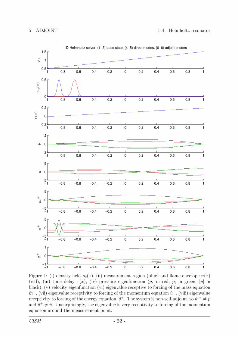
Figure 1: (i) density field ρ0(x), (ii) measurement region (blue) and flame envelope n(x)(red), (iii) time delay τ(x), (iv) pressure eigenfunction (pr in red, pi in green, |p| inblack), (v) velocity eigenfunction (vi) eigenvalue receptive to forcing of the mass equationm+, (vii) eigenvalue receptivity to forcing of the momentum equation u+, (viii) eigenvaluereceptivity to forcing of the energy equation, q+. The system is non-self-adjoint, so m+ 6= pand u+ 6= u. Unsurprisingly, the eigenvalue is very receptivity to forcing of the momentumequation around the measurement point.
CISM - 22 -
5.4 Helmholtz resonator 5 ADJOINT
−1 −0.5 0 0.5 1−0.3
−0.2
−0.1
0
0.1
0.2
0.3
0.4
...
to m
ass e
q.
from u ...
δ freq
δ g.rate
−1 −0.5 0 0.5 1−0.2
0
0.2
0.4
0.6
0.8from p ...
δ freq
δ g.rate
−1 −0.5 0 0.5 1−0.8
−0.6
−0.4
−0.2
0
0.2
0.4
0.6
...
to m
om
en
tum
eq
.
δ freq
δ g.rate
−1 −0.5 0 0.5 1−0.4
−0.3
−0.2
−0.1
0
0.1
0.2
0.3
δ freq
δ g.rate
−1 −0.5 0 0.5 1−0.1
−0.05
0
0.05
0.1
...
to e
ne
rgy e
q.
δ freq
δ g.rate
−1 −0.5 0 0.5 1−0.05
0
0.05
0.1
0.15
0.2
0.25
0.3
δ freq
δ g.rate
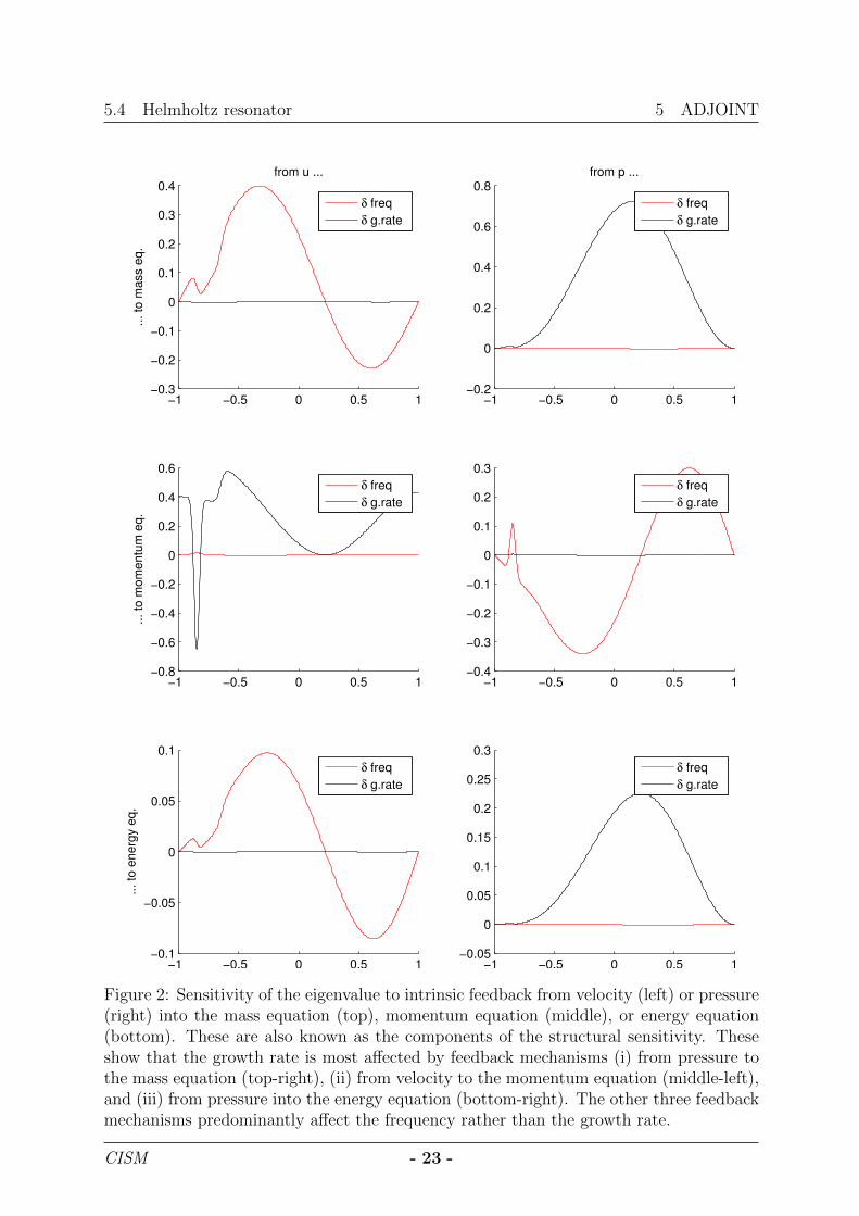
Figure 2: Sensitivity of the eigenvalue to intrinsic feedback from velocity (left) or pressure(right) into the mass equation (top), momentum equation (middle), or energy equation(bottom). These are also known as the components of the structural sensitivity. Theseshow that the growth rate is most affected by feedback mechanisms (i) from pressure tothe mass equation (top-right), (ii) from velocity to the momentum equation (middle-left),and (iii) from pressure into the energy equation (bottom-right). The other three feedbackmechanisms predominantly affect the frequency rather than the growth rate.
CISM - 23 -
5 ADJOINT 5.5 The influence of a passive drag device
constant calculated from the geometry of the resonator. This influence is shown in figure3
It might sound reasonable to assume that the best place to put a Helmholtz resonatoris at the pressure anti-node. This would indeed be true if thermo-acoustic systems wereself-adjoint, as are acoustic systems, because the sensitivity of the mass equation, m+,would then be identical to the pressure eigenfunction, p. In a thermo-acoustic system,however, m+ differs from p. The best place to put a Helmholtz resonator is where theproduct of m+ and p is maximal.
5.5 The influence of a passive drag device
A passive drag device, such as a mesh, forces the flow in the opposite direction to theinstantaneous velocity. Provided that the velocity perturbation is small compared withthe mean velocity, the force is linearly proportional to the velocity:
f = −CD ×1
2ρUu (126)
where CD is the drag coefficient of the mesh. This influence is shown in figure 4
Exercise In solid rocket engines, the reaction rate of the fuel increases as the localpressure increases. With reference to figure 2 explain whether or not you expect solidrocket engines to be susceptible to thermoacoustic oscillations.
Exercise Use the structural sensitivity to estimate the influence that the momentumboundary layer has on the growth rate of the eigenvalue.
Exercise Use the structural sensitivity to estimate the influence that the thermal bound-ary layer has on the growth rate of the eigenvalue.
5.6 Sensitivity of the eigenvalue to changes in the base state
We start from the unperturbed problem with no external feedback (88)
(DRD−NΦF) p = +σAp, (127)
where R contains 1/ρ0 along the diagonal, N contains nu(x) along the diagonal, Φ containsexp(iωτu(x)) along the diagonal and F is the measurement matrix. If we define L ≡DRD−NΦF then we see that
δL = D(δR)D− (δN)ΦF−N(δΦ)F−NΦ(δF) (128)
(The matrix A can depend on the boundary conditions but we will not consider changesto the boundary conditions in this tutorial.) Therefore the shift in the eigenvalue δσ fora change in nu(x) is given by:
δσ = −(p+)HMδNΦFp
(p+)HMAp(129)
CISM - 24 -

5.6 Base state sensitivity 5 ADJOINT
−1 −0.8 −0.6 −0.4 −0.2 0 0.2 0.4 0.6 0.8 1−2
0
2
p
Sh i f t in e igenvalue c aused by He lmholtz re sonator at x
−1 −0.8 −0.6 −0.4 −0.2 0 0.2 0.4 0.6 0.8 1−1
0
1
m+
−1 −0.8 −0.6 −0.4 −0.2 0 0.2 0.4 0.6 0.8 1−150
−100
−50
0
δ g
.rate
−1 −0.8 −0.6 −0.4 −0.2 0 0.2 0.4 0.6 0.8 10
10
20
30
δ fre
q.
Figure 3: (i) pressure eigenfunction (pr in red, pi in green, |p| in black), (ii) receptivity ofthe eigenvalue to forcing of the mass equation, m+, (iii) sensitivity of the growth rate to aHelmholtz resonator placed at position x, (iv) sensitivity of the frequency to a Helmholtzresonator. A common assumption is that a Helmholtz resonator most reduces the growthrate where p2 is largest. However, this analysis shows that it actually has most influencewhere the product pm+ is largest and, furthermore, that p 6= m+ because, unlike anacoustic system, the thermoacoustic system is not self-adjoint.
CISM - 25 -

5 ADJOINT 5.6 Base state sensitivity
−1 −0.8 −0.6 −0.4 −0.2 0 0.2 0.4 0.6 0.8 1−1
0
1
u
Sh i f t in e igenvalue c aused by a gauz e at x
−1 −0.8 −0.6 −0.4 −0.2 0 0.2 0.4 0.6 0.8 1−2
0
2
u+
−1 −0.8 −0.6 −0.4 −0.2 0 0.2 0.4 0.6 0.8 1−1
0
1
δ g
.ra
te
−1 −0.8 −0.6 −0.4 −0.2 0 0.2 0.4 0.6 0.8 1−0.04
−0.02
0
0.02
δ f
req
.
Figure 4: (i) velocity eigenfunction (ur in red, ui in green, |u| in black), (ii) receptivity ofthe eigenvalue to forcing of the momentum equation, m+, (iii) sensitivity of the growthrate to a drag device placed at position x, (iv) sensitivity of the frequency to a drag device.
CISM - 26 -
5.7 Convergence check (the Taylor test) 6 SUMMARY
We can either specify δnu(x) and then calculate δσ or, more usefully, calculate the function
δσ = −((p+)HM)T × ΦFp
(p+)HMAp(130)
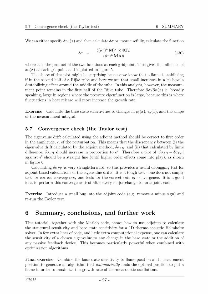
where × is the product of the two functions at each gridpoint. This gives the influence ofδn(x) at each gridpoint and is plotted in figure 5.
The shape of this plot might be surprising because we know that a flame is stabilizingif in the second half of a Rijke tube and here we see that small increases in n(x) have adestabilizing effect around the middle of the tube. In this analysis, however, the measure-ment point remains in the first half of the Rijke tube. Therefore ∂σ/∂n(x) is, broadlyspeaking, large in regions where the pressure eigenfunction is large, because this is wherefluctuations in heat release will most increase the growth rate.
Exercise Calculate the base state sensitivities to changes in ρ0(x), τn(x), and the shapeof the measurement integral.
5.7 Convergence check (the Taylor test)
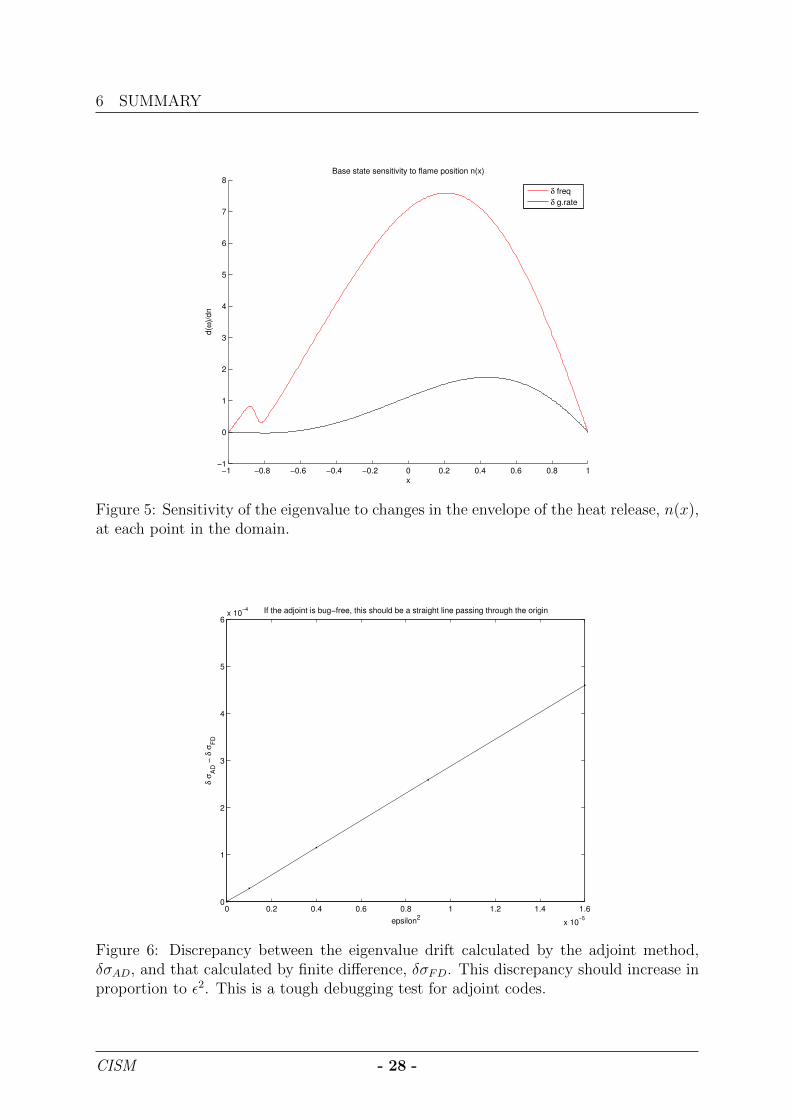
The eigenvalue drift calculated using the adjoint method should be correct to first orderin the amplitude, ε, of the perturbation. This means that the discrepancy between (i) theeigenvalue drift calculated by the adjoint method, δσAD, and (ii) that calculated by finitedifference, δσFD should increase in proportion to ε2. Therefore a plot of |δσAD − δσFD|against ε2 should be a straight line (until higher order effects come into play), as shownin figure 6.
Calculating δσFD is very straightforward, so this provides a useful debugging test foradjoint-based calculations of the eigenvalue drifts. It is a tough test - one does not simplytest for correct convergence; one tests for the correct rate of convergence. It is a goodidea to perform this convergence test after every major change to an adjoint code.
Exercise Introduce a small bug into the adjoint code (e.g. remove a minus sign) andre-run the Taylor test.
6 Summary, conclusions, and further work
This tutorial, together with the Matlab code, shows how to use adjoints to calculatethe structural sensitivity and base state sensitivity for a 1D thermo-acoustic Helmholtzsolver. In few extra lines of code, and little extra computational expense, one can calculatethe sensitivity of a chosen eigenvalue to any change in the base state or the addition ofany passive feedback device. This becomes particularly powerful when combined withoptimization algorithms.
Final exercise Combine the base state sensitivity to flame position and measurementposition to generate an algorithm that automatically finds the optimal position to put aflame in order to maximize the growth rate of thermoacoustic oscillations.
CISM - 27 -
6 SUMMARY
−1 −0.8 −0.6 −0.4 −0.2 0 0.2 0.4 0.6 0.8 1−1
0
1
2
3
4
5
6
7
8
x
d(ω
)/dn
Base state sensitivity to flame position n(x)
δ freq
δ g.rate
Figure 5: Sensitivity of the eigenvalue to changes in the envelope of the heat release, n(x),at each point in the domain.
0 0.2 0.4 0.6 0.8 1 1.2 1.4 1.6
x 10−5
0
1
2
3
4
5
6x 10
−4
epsilon2
δ σ
AD
− δ
σF
D
If the adjoint is bug−free, this should be a straight line passing through the origin
Figure 6: Discrepancy between the eigenvalue drift calculated by the adjoint method,δσAD, and that calculated by finite difference, δσFD. This discrepancy should increase inproportion to ε2. This is a tough debugging test for adjoint codes.
CISM - 28 -

REFERENCES REFERENCES
References
Chandler, G. J. (2010). Sensitivity analysis of low-density jets and flames. PhD thesis,University of Cambridge.
Chomaz, J.-M. (1993). Linear and non-linear, local and global stability analysis of openflows. Turbulence in spatially extended systems, pages 245–257.
Chomaz, J.-M. (2005). Global instabilities in spatially developing flows: Non-Normalityand Nonlinearity. Annual Review of Fluid Mechanics, 37:357–392.
Cossu, C. (2014). An introduction to optimal controllecture notes from the flow-norditasummer school on advanced instability methods for complex flows, stockholm, sweden,2013. Applied Mechanics Reviews, 66(2):024801–024801.
Culick, F. E. C. (2006). Unsteady motions in combustion chambers for propulsion systems.RTO AGARDograph AG-AVT-039, North Atlantic Treaty Organization.
Dennery, P. and Krzywicky, A. (1996). Mathematics for Physicists. Dover Publications,Inc.
Dowling, A. P. and Ffowcs-Williams, J. E. (1983). Sound and Sources of Sound. Horwood.
Giannetti, F. and Luchini, P. (2007). Structural sensitivity of the first instability of thecylinder wake. Journal of Fluid Mechanics, 581:167–197.
Hill, D. C. (1992a). A theoretical approach for analyzing the re-stabilization of wakes.AIAA Paper, pages 67–92.
Hill, D. C. (1992b). A theoretical approach for analyzing the restabilization of wakes.NASA Technical memorandum 103858.
Hill, D. C. (1995a). Adjoint systems and their role in the receptivity problem for boundarylayers. J. Fluid Mech., 292:183–204.
Hill, D. C. (1995b). Adjoint systems and their role in the receptivity problem for boundarylayers. Journal of Fluid Mechanics, 292:183–204.
Hinch, E. J. (1991). Perturbation Methods. Cambridge University Press.
Huerre, P. and Monkewitz, P. (1990). Local and global instabilities of spatially developingflows. Ann. Rev. Fluid Mech., 22:473–537.
Kato, T. (1980). Perturbation theory for linear operators. Springer Berlin / Heidelberg,New York, 2nd edition.
Lieuwen, T. C. (2012). Unsteady combustor physics. Cambridge University Press.
Luchini, P. and Bottaro, A. (2014). Adjoint equations in stability analysis. Ann. Rev.Fluid Mech., 46:1–30.
CISM - 29 -
REFERENCES REFERENCES
Maddox, I. J. (1988). Elements of Functional Analysis. Cambridge University Press, 2ndedition.
Magri, L. and Juniper, M. P. (2013). Sensitivity analysis of a time-delayed thermo-acousticsystem via an adjoint-based approach. Journal of Fluid Mechanics, 719:183–202.
Marino, L. and Luchini, P. (2009). Adjoint analysis of the flow over a forward-facing step.Theoretical and Computational Fluid Dynamics, 23(1):37–54.
Marquet, O., Sipp, D., and Jacquin, L. (2008). Sensitivity analysis and passive control ofcylinder flow. Journal of Fluid Mechanics, 615:221–252.
Meliga, P., Chomaz, J.-M., and Sipp, D. (2009). Unsteadiness in the wake of disks andspheres: Instability, receptivity and control using direct and adjoint global stabilityanalyses. Journal of Fluids and Structures, 25(4):601–616.
Nicoud, F., Benoit, L., Sensiau, C., and Poinsot, T. (2007). Acoustic modes in com-bustors with complex impedances and multidimensional active flames. AIAA Journal,45(2):426–441.
Oden, J. T. (1979). Applied functional analysis. Prentice-Hall, Inc.
Qadri, U. A., Mistry, D., and Juniper, M. P. (2013). Structural sensitivity of spiral vortexbreakdown. Journal of Fluid Mechanics, page to appear.
Rayleigh (1878). The explanation of certain acoustical phenomena. Nature, 18:319–321.
Rayleigh, L. (1880). On the stability and instability of certain fluid motions. Proc. Lond.Maths. Soc., 11:57–70.
Salwen, H. and Grosch, C. E. (1981). The continuous spectrum of the Orr-Sommerfeldequation. Part 2. Eigenfunction expansions. Journal of Fluid Mechanics, 104:445–465.
Schmid, P. J. and Brandt, L. (2014). Analysis of fluid systems: Stability, receptivity,sensitivity. Applied Mechanics Review, 66:024803–1–21.
Sipp, D., Marquet, O., Meliga, P., and Barbagallo, A. (2010). Dynamics and Controlof Global Instabilities in Open-Flows: A Linearized Approach. Applied MechanicsReviews, 63(3):030801.
Stewart, G. W. and Sun, J.-G. (1990). Matrix Perturbation Theory. Academic press, Inc.
Trefethen, L. N. (2000). Spectral Methods in Matlab. SIAM.
CISM - 30 -