ADELE: Anomaly Detection from Event LogEmpiricism

Subhendu Khatuya∗, Niloy Ganguly∗, Jayanta Basak†, Madhumita Bharde†, Bivas Mitra∗∗Department of Computer Science and Engineering, Indian Institute of Technology Kharagpur, INDIA 721302

†NetApp Inc., Bangalore, IndiaEmail: subhendu.cse@iitkgp.ac.in, niloy@cse.iitkgp.ernet.in, Jayanta.Basak@netapp.com,

madhumita.bharde@gmail.com, bivas@cse.iitkgp.ernet.in

Abstract—A large population of users gets affected by suddenslowdown or shutdown of an enterprise application. Systemadministrators and analysts spend considerable amount of timedealing with functional and performance bugs. These problemsare particularly hard to detect and diagnose in most computersystems, since there is a huge amount of system generatedsupportability data (counters, logs etc.) that need to be analyzed.Most often, there isn’t a very clear or obvious root cause. Timelyidentification of significant change in application behavior is veryimportant to prevent negative impact on the service. In this paper,we present ADELE, an empirical, data-driven methodology forearly detection of anomalies in data storage systems. The keyfeature of our solution is diligent selection of features from systemlogs and development of effective machine learning techniquesfor anomaly prediction. ADELE learns from system’s own historyto establish the baseline of normal behavior and gives accurateindications of the time period when something is amiss for asystem. Validation on more than 4800 actual support cases shows∼ 83% true positive rate and ∼ 12% false positive rate inidentifying periods when the machine is not performing normally.We also establish the existence of problem “signatures” whichhelp map customer problems to already seen issues in the field.ADELE’s capability to predict early paves way for online failureprediction for customer systems.

Index Terms—System Log; Anomaly Detection

I. INTRODUCTION

Reliable and fast support service in times of failure is aprerequisite for an efficient storage facility. Enterprise storagesystems are typically used for mission-critical business ap-plications. Customers consistently rely on storage vendors toprovide high availability of data. Although failures cannot becompletely avoided, a 24x7 support service that helps resolveissues within minimum case resolution time1 is an imperative.

For efficient diagnosis of failures, complex enterprise sys-tems have instrumentation to generate massive amounts oftelemetry data everyday - typically in the form of counters,logs etc. When customer reports a problem (by opening a“support case”) in the field, a support engineer with domainexpertise tends to sift through weeks or even months oftelemetry information to identify something abnormal. Theytypically rely on thumb rules (e.g. severity-based filteringfor logs) or prior experience to identify relevant entries andthereby eventually, the root cause. However, our analysis (in

1Case resolution period is the duration between ‘Case opened date’ and‘Case closed date’ from customer support database.

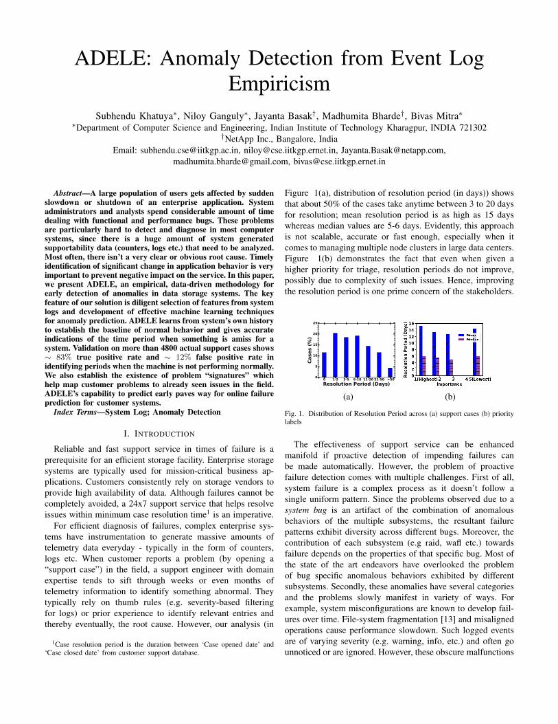
Figure 1(a), distribution of resolution period (in days)) showsthat about 50% of the cases take anytime between 3 to 20 daysfor resolution; mean resolution period is as high as 15 dayswhereas median values are 5-6 days. Evidently, this approachis not scalable, accurate or fast enough, especially when itcomes to managing multiple node clusters in large data centers.Figure 1(b) demonstrates the fact that even when given ahigher priority for triage, resolution periods do not improve,possibly due to complexity of such issues. Hence, improvingthe resolution period is one prime concern of the stakeholders.

0 1-2 3-5 6-10 11-20 21-50 >50

Resolution Period (Days)

0

5

10

15

20

25

Cases (%)

(a) (b)

Fig. 1. Distribution of Resolution Period across (a) support cases (b) prioritylabels

The effectiveness of support service can be enhancedmanifold if proactive detection of impending failures canbe made automatically. However, the problem of proactivefailure detection comes with multiple challenges. First of all,system failure is a complex process as it doesn’t follow asingle uniform pattern. Since the problems observed due to asystem bug is an artifact of the combination of anomalousbehaviors of the multiple subsystems, the resultant failurepatterns exhibit diversity across different bugs. Moreover, thecontribution of each subsystem (e.g raid, wafl etc.) towardsfailure depends on the properties of that specific bug. Most ofthe state of the art endeavors have overlooked the problemof bug specific anomalous behaviors exhibited by differentsubsystems. Secondly, these anomalies have several categoriesand the problems slowly manifest in variety of ways. Forexample, system misconfigurations are known to develop fail-ures over time. File-system fragmentation [13] and misalignedoperations cause performance slowdown. Such logged eventsare of varying severity (e.g. warning, info, etc.) and often gounnoticed or are ignored. However, these obscure malfunctions

from one subsystem propagate and cascade to others andresult in an undesirable behavior from an overall system orapplication perspective. Thirdly, their is a subtle differencebetween anomaly and failures observed. During operation,subsystems or modules might exhibit anomaly such as systemslowdown due to heavy load, increase response time of storageI/O, however that may not always necessarily lead to failure.Proper handling of those (false) signals is important as thismay raise a large numbers of false positive alerts which mayslower the utility of the failure prediction system. This papertakes an important step towards this direction.

In terms of data sources for anomaly identification, countersand logs provide different value propositions. Counters are col-lected periodically while logs have event driven characteristics.In general, system performance issues can be better diagnosedwith the help of counters [11] [10]. On the other hand, for is-sues like system misconfiguration or component failures, logscontain valuable signals for prediction of anomalies [12][8][2].There have been several studies on anomaly detection from thelog files; for instance Liang et al [9] proposed the methodologyto forecast the fatal event from IBM Bluegene/L logs. Jianget al [5] provided interesting data-driven analysis of customerproblem troubleshooting for around 100000 field systems.Shatnawi et al [14] proposed a framework for predicting onlineservice failure based on production logs.This paper effectively highlights the challenges of the noisylog events and conducts an extensive log analysis to uncoverthe anomaly signatures. We start with background about cus-tomer support infrastructure and data selection criteria (SectionII). Subsequently, we develop ADELE, which leverages onthe machine learning techniques to (a) predict system failurein advance by analyzing of log data and anomaly signaturesgenerated by different modules (Section IV) and (b) developan automated early warning mechanism to protect the systemfrom catastrophe. In case of a massive failure, the final failureis typically preceded by a sequence of small malfunctions,which most of the time have been overlooked. However, ifcorrectly diagnosed at proper time, these apparently harmlessmalfunctioning signals can predict, in advance, the occur-rence of a big failure. The novelty of ADELE is manifold(a) ADELE captures the uniqueness of the individual bugs;while detecting the anomaly, it considers and estimates the(varying) responsibility of the individual subsystems causingthe problem (b) instead of merely relying on the vanilla fea-tures for anomaly detection, ADELE observes the abnormalityexhibited by the individual features (via outlier detection)to compute the anomaly score (c) finally, through empiricalexperiments, we discriminate the failures with the anomaly,which substantially reduces the false alarms.We show that ADELE outperforms the baseline with 83% Truepositive and 12% False Positive rate. It should be noted thatthe log analysis method presented here is a black-box methodand does not tie itself to any domain-specific context.

In a nutshell, ADELE makes following major contributions:• A comprehensive and generic abstraction of storage

system logs based on their metadata characteristics is

Field Log Entry Example DescriptionEvent Time Sat Aug 17 09:11:12 PDT Day, date, timestamp and timezone

System name cc-nas1 Name of the node in cluster thatgenerated the event

Event ID filesystem1.scan.start EMS event ID. Contains Subsystemname and event type

Severity info {Severity of the event}

Message String Starting block reallocation onaggregate aggr0 Message string with argument values

TABLE IEMS MESSAGE STRUCTURE

developed (Section III).• Through detailed study and rigorous analysis, the rela-

tionship between anomaly signals and failure is estab-lished. Problem-specific models are learnt using machinelearning techniques and accuracy is demonstrated withlarge number of customer support cases (Section V).

• Problem specific models and signatures are extended forgeneric failure prediction by mapping unknown problemsto already seen issues in field. More importantly, ADELEcreates groundwork for an proactive, online failure pre-diction (Section VI).

II. BACKGROUND AND DATASET

A. Auto Support

System generated data like counters, logs and commandhistory etc. are critical for troubleshooting of customer issues.Auto Support (ASUP) infrastructure provides an ability toforward this logged data (storage system log) daily to Ne-tApp. While customers can opt out of this facility, most ofthem choose to go for it since it provides proactive systemmonitoring capabilities and faster customer support.

B. Event Message System (EMS) Logs

Support infrastructure described above gives access to dailyEMS logs2. An example of a typical EMS log entry is asfollows:Sat Aug 17 09:11:12 PDT [cc-nas1:filesystem1.scan.start:info]: Starting block reallocationon aggregate aggr0.Interpretation of fields is summarized in Table I in contextof the above log entry. Each log entry contains time of theevent with fields like day, date, timestamp and timezone. Asmultiple systems (alternatively, storage “nodes”) are clusteredin a typical Data ONTAP R© setup, name of the node whereevent occurred within the cluster is required to be part of thelog entry. Event ID gives information about the kind of eventthat occurred in an hierarchical fashion. First part of this ID isthe subsystem that generated the event. Severity field can takea value from ‘emergency’, ‘alert’, ‘critical’, ‘error’, ‘warning’,‘notice’, ‘info’, ‘debug’. Message string throws more light onthe event by incorporating context-specific argument values(e.g. ‘aggr0’ from above example) for describing the event.

2https://library.netapp.com/ecmdocs/ECMP1196817/html/event/log/show.html

C. Customer Support Database and Bug Database

Customer Support Database: Customer support portalprovides customers an ability to report their grievances. Italso provides a forum for customers to engage with supportengineers to clarify configuration queries and provide otherguidance. Cases can be system generated based on predefinedrules or human-generated. We query this database for fieldslike opened date, closed date, priority label etc. for customersupport cases.

Bug database: Bug database is typically internally orientedand tracks the engineering side of problems. The same bugcan be experienced across multiple customers, systems andconfigurations. We use this database to query customer casesassociated with bugs.

D. Data Filtering

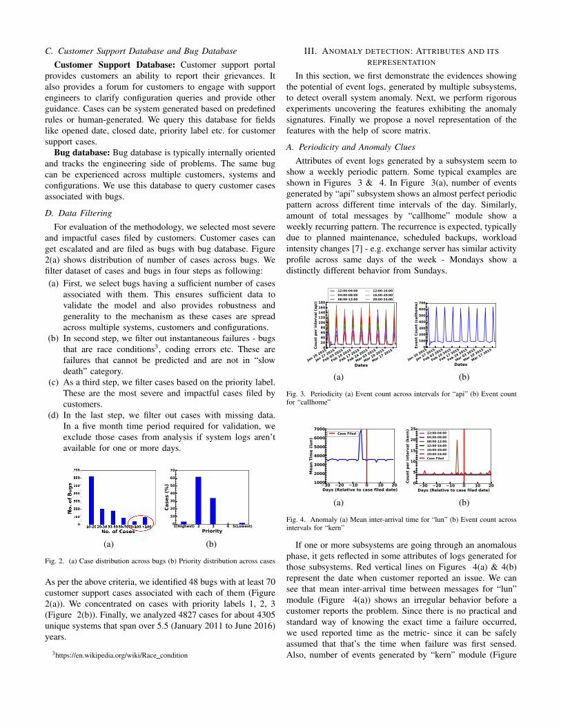
For evaluation of the methodology, we selected most severeand impactful cases filed by customers. Customer cases canget escalated and are filed as bugs with bug database. Figure2(a) shows distribution of number of cases across bugs. Wefilter dataset of cases and bugs in four steps as following:(a) First, we select bugs having a sufficient number of cases

associated with them. This ensures sufficient data tovalidate the model and also provides robustness andgenerality to the mechanism as these cases are spreadacross multiple systems, customers and configurations.

(b) In second step, we filter out instantaneous failures - bugsthat are race conditions3, coding errors etc. These arefailures that cannot be predicted and are not in “slowdeath” category.

(c) As a third step, we filter cases based on the priority label.These are the most severe and impactful cases filed bycustomers.

(d) In the last step, we filter out cases with missing data.In a five month time period required for validation, weexclude those cases from analysis if system logs aren’tavailable for one or more days.

1(Highest) 2 3 4 5(Lowest)

Priority

0

10

20

30

40

50

60

70

Cases (%)

(a) (b)

Fig. 2. (a) Case distribution across bugs (b) Priority distribution across cases

As per the above criteria, we identified 48 bugs with at least 70customer support cases associated with each of them (Figure2(a)). We concentrated on cases with priority labels 1, 2, 3(Figure 2(b)). Finally, we analyzed 4827 cases for about 4305unique systems that span over 5.5 (January 2011 to June 2016)years.

3https://en.wikipedia.org/wiki/Race condition

III. ANOMALY DETECTION: ATTRIBUTES AND ITSREPRESENTATION

In this section, we first demonstrate the evidences showingthe potential of event logs, generated by multiple subsystems,to detect overall system anomaly. Next, we perform rigorousexperiments uncovering the features exhibiting the anomalysignatures. Finally we propose a novel representation of thefeatures with the help of score matrix.

A. Periodicity and Anomaly Clues

Attributes of event logs generated by a subsystem seem toshow a weekly periodic pattern. Some typical examples areshown in Figures 3 & 4. In Figure 3(a), number of eventsgenerated by “api” subsystem shows an almost perfect periodicpattern across different time intervals of the day. Similarly,amount of total messages by “callhome” module show aweekly recurring pattern. The recurrence is expected, typicallydue to planned maintenance, scheduled backups, workloadintensity changes [7] - e.g. exchange server has similar activityprofile across same days of the week - Mondays show adistinctly different behavior from Sundays.

Jan 20

2015

Jan 27

2015

Feb 0

3 2015

Feb 1

0 2015

Feb 1

7 2015

Feb 2

4 2015

Mar 0

3 2015

Mar 1

0 2015

Mar 1

7 2015

Dates

0

20

40

60

80

100

120

140

160

180

Count per interval (api)

12:00-04:00

04:00-08:00

08:00-12:00

12:00-16:00

16:00-20:00

20:00-24:00

Jan 20

2015

Jan 27

2015

Feb 0

3 2015

Feb 1

0 2015

Feb 1

7 2015

Feb 2

4 2015

Mar 0

3 2015

Mar 1

0 2015

Mar 1

7 2015

Dates

0

100

200

300

400

500

600

700

Event Count (callhome)

(a) (b)

Fig. 3. Periodicity (a) Event count across intervals for “api” (b) Event countfor “callhome”

−30 −20 −10 0 10 20Days (Relative to case filed date)

1000

2000

3000

4000

5000

6000

7000

Mean Tim

e (lun)

Case Filed

−30 −20 −10 0 10 20Days (Relati e to case filed date)

0

5

10

15

20

25

Count per inter al (kern)

12:00-04:00

04:00-08:00

08:00-12:00

12:00-16:00

16:00-20:00

20:00-24:00

Case Filed

(a) (b)

Fig. 4. Anomaly (a) Mean inter-arrival time for “lun” (b) Event count acrossintervals for “kern”

If one or more subsystems are going through an anomalousphase, it gets reflected in some attributes of logs generated forthose subsystems. Red vertical lines on Figures 4(a) & 4(b)represent the date when customer reported an issue. We cansee that mean inter-arrival time between messages for “lun”module (Figure 4(a)) shows an irregular behavior before acustomer reports the problem. Since there is no practical andstandard way of knowing the exact time a failure occurred,we used reported time as the metric- since it can be safelyassumed that that’s the time when failure was first sensed.Also, number of events generated by “kern” module (Figure

4(b)) across different intervals in the day shows an abnormalbehavior few days prior to case filed date. A system failure istypically preceded by one or more modules generating eventsin patterns that are not “normal”4.

B. Engineering Log AttributesEMS logs have a total of approximately 7800 event types

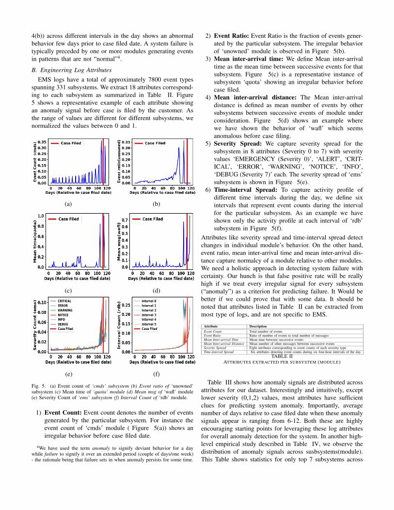
spanning 331 subsystems. We extract 18 attributes correspond-ing to each subsystem as summarized in Table II. Figure5 shows a representative example of each attribute showingan anomaly signal before case is filed by the customer. Asthe range of values are different for different subsystems, wenormalized the values between 0 and 1.

(a) (b)

(c) (d)

(e) (f)

Fig. 5. (a) Event count of ‘cmds’ subsystem (b) Event ratio of ‘unowned’subsystem (c) Mean time of ‘quota’ module (d) Mean msg of ‘wafl’ module(e) Severity Count of ‘ems’ subsystem (f) Interval Count of ‘rdb’ module.

1) Event Count: Event count denotes the number of eventsgenerated by the particular subsystem. For instance theevent count of ‘cmds’ module ( Figure 5(a)) shows anirregular behavior before case filed date.

4We have used the term anomaly to signify deviant behavior for a daywhile failure to signify it over an extended period (couple of days/one week)- the rationale being that failure sets in when anomaly persists for some time.

2) Event Ratio: Event Ratio is the fraction of events gener-ated by the particular subsystem. The irregular behaviorof ‘unowned’ module is observed in Figure 5(b).

3) Mean inter-arrival time: We define Mean inter-arrivaltime as the mean time between successive events for thatsubsystem. Figure 5(c) is a representative instance ofsubsystem ‘quota’ showing an irregular behavior beforecase filed.

4) Mean inter-arrival distance: The Mean inter-arrivaldistance is defined as mean number of events by othersubsystems between successive events of module underconsideration. Figure 5(d) shows an example wherewe have shown the behavior of ‘wafl’ which seemsanomalous before case filing.

5) Severity Spread: We capture severity spread for thesubsystem in 8 attributes (Severity 0 to 7) with severityvalues ‘EMERGENCY (Severity 0)’, ‘ALERT’, ‘CRIT-ICAL’, ‘ERROR’, ‘WARNING’, ‘NOTICE’, ‘INFO’,‘DEBUG (Severity 7)’ each. The severity spread of ‘ems’subsystem is shown in Figure 5(e).

6) Time-interval Spread: To capture activity profile ofdifferent time intervals during the day, we define sixintervals that represent event counts during the intervalfor the particular subsystem. As an example we haveshown only the activity profile at each interval of ‘rdb’subsystem in Figure 5(f).

Attributes like severity spread and time-interval spread detectchanges in individual module’s behavior. On the other hand,event ratio, mean inter-arrival time and mean inter-arrival dis-tance capture normalcy of a module relative to other modules.We need a holistic approach in detecting system failure withcertainty. Our hunch is that false positive rate will be reallyhigh if we treat every irregular signal for every subsystem(“anomaly”) as a criterion for predicting failure. It Would bebetter if we could prove that with some data. It should benoted that attributes listed in Table II can be extracted frommost type of logs, and are not specific to EMS.

Attribute DescriptionEvent Count Total number of eventsEvent Ratio Ratio of number of events to total number of messagesMean Inter-arrival Time Mean time between successive eventsMean Inter-arrival Distance Mean number of other messages between successive eventsSeverity Spread Eight attributes corresponding to event counts of each severity typeTime-interval Spread Six attributes denoting event counts during six four-hour intervals of the day

TABLE IIATTRIBUTES EXTRACTED PER SUBSYSTEM (MODULE)

Table III shows how anomaly signals are distributed acrossattributes for our dataset. Interestingly and intuitively, exceptlower severity (0,1,2) values, most attributes have sufficientclues for predicting system anomaly. Importantly, averagenumber of days relative to case filed date when these anomalysignals appear is ranging from 6-12. Both these are highlyencouraging starting points for leveraging these log attributesfor overall anomaly detection for the system. In another high-level empirical study described in Table IV, we observe thedistribution of anomaly signals across susbsystems(module).This Table shows statistics for only top 7 subsystems across

Attribute Cases(%)

TotalSignals

AverageDays

Event Count 68.39 7163 10.86Event Ratio 66.25 7037 11.01

Mean Inter-arrival Time 80.30 12955 9.90Mean Inter-arrival Distance 66.10 9816 11.08

Severity 0 0.00 0.00 0.00Severity 1 0.30 14 10.0Severity 2 0.00 0.00 0.00Severity 3 8.39 456 11.88Severity 4 14.65 773 10.91Severity 5 12.06 648 11.23Severity 6 34.04 2203 10.91Severity 7 42.59 3124 12.89Interval 1 46.87 4016 7.25Interval 2 44.58 3249 9.95Interval 3 48.24 4045 10.76Interval 4 47.63 3854 6.80Interval 5 52.06 4178 11.67Interval 6 49.00 4289 12.13

TABLE IIIDISTRIBUTION OF ANOMALY CLUES ACROSS ALL CASES. NOTE THATEXCEPT LOWER SEVERITY VALUES (0,1,2), MOST ATTRIBUTES SHOW

SUFFICIENT CLUES.

all log attributes described earlier. Reasonably high number ofcases show subsystems in anomalous conditions considerablyearly from the case filed date.

Subsystem Cases (%) TotalSignals

AverageDays

raid 13.03 8842 10.82kern 11.51 7811 10.98wafl 7.95 5394 11.01ems 7.12 4834 11.10

callhome 7.09 4811 7.26disk 5.21 3537 10.87

hamsg 3.94 2674 10.92TABLE IV

DISTRIBUTION OF ANOMALY SIGNALS ACROSS SUBSYSTEMS.

C. Representation of Features: Log Transformation

Extracted 18 attributes corresponding to each subsystem(module) per day is summarized in Table II. We call eachModule-attribute combination as “feature”. First, we representEMS log of dth day as a raw feature matrix as follows.

Xd ={X

(d)i,j where i ∈M and j ∈ A

}where M is the set of modules (|M | = m) and A is the set ofattributes (|A| = a). ith row and jth column of Xd containsjth attribute’s value of ith subsystem.

IV. ADELE: FRAMEWORK FOR ANOMALY DETECTION

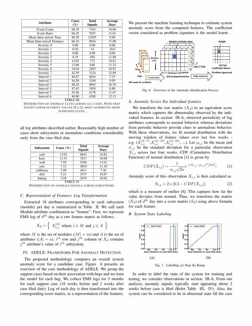
The proposed methodology computes an overall systemanomaly score for a candidate case. Figure 6 presents anoverview of the core methodology of ADELE. We group thesupport cases based on their association with bugs and we trainthe model for each bug. We collect EMS logs for 5 monthsfor each support case (18 weeks before and 2 weeks aftercase filed date). Log of each day is then transformed into thecorresponding score matrix, as a representation of the features.

We present the machine learning technique to estimate systemanomaly score from the computed features. The coefficientvector considered as problem signature is the model learnt.

Fig. 6. Overview of the Anomaly identification Process

A. Anomaly Scores For Individual features

We transform the raw matrix (Xd) to an equivalent scorematrix which captures the abnormality observed by the indi-vidual features. In section III-A, observed periodicity of logattributes corresponds to normal behavior whereas deviationsfrom periodic behavior provide clues to anomalous behavior.With these observations, we fit normal distribution with themoving window of feature values over last few weeks -e.g. (X(d−7)

i,j ,X(d−14)i,j ,X(d−21)

i,j , ...). Let µi,j be the mean andσi,j be the standard deviation for a particular observationXi,j across last four weeks. CDF (Cumulative DistributionFunction) of normal distribution [1] is given by

CDF (Xi,j) =1

σi,j√2πe−(Xi,j−µi,j)

2/2σ2i,j (1)

Anomaly score of this observation Xi,j is then calculated as

Si,j = 2 ∗ |0.5− CDF (Xi,j)| (2)

which is a measure of outlier [4]. This captures how far thevalue deviates from normal. Thus, we transform the matrix(Xd) of dth day into a score matrix (Sd) using above formulafor each feature.

B. System State Labeling

−98 −70 −42 −14 0 7Days (Relative to case filed date)

0.0

0.2

0.4

0.6

0.8

1.0

Label

Case Filed

−98 −70 −42 −14 0 7Days (Relative to case filed date)

0.0

0.2

0.4

0.6

0.8

1.0

Label

Case Filed

(a) (b)

Fig. 7. Labelling (a) Step (b) Ramp.

In order to label the state of the system for training andtesting, we consider observations in section III-A. From ouranalysis, anomaly signals typically start appearing about 2weeks before case is filed (Refer Table III, IV). Also, thesystem can be considered to be in abnormal state till the case

is resolved (refer Figure 1, median case resolution time is 5-6days.) With these data-driven insights, we label 2 weeks beforeand 1 week after case filed date as an abnormal period. Heredata produced in each of those days are marked as anomalous.Rest of the days are treated as normal. In Figure 7, weconsider two types of labeling strategy (a) Step and (b) Ramp.In step labeling, we assign a score of either 0 (normal) or1(abnormal). In case of ramp labeling, system state of each dayis annotated with a fractional number, the number is inverselyproportional to the number of days before failure set in - thatis further the day is from failure smaller is the value assigned.

C. Estimating System Anomaly Score

We develop ADELE to compute the overall anomaly scorefrom the feature vector represented as the score matrix Sd.Each feature (Si,j) contributes differently to overall anomalyof the system depending upon the specific problem. Forinstance, disk subsystem might be highly anomalous for someproblems but not for others. In essence, these contributionsare problem-specific and are learnt using Ridge regression.Two labelling strategies as described in section IV-B are usedfor learning. We perform learning using Ridge regression5

which minimizes squared error while regularizing the norm ofthe weights. It performs better as compared to other methodsbecause of its inherent mechanisms to address the possibilityof multi-collinearity and sparseness of coefficients which istypical in our dataset. The weight vector (w) of length m ∗ areturned by Ridge regression is termed as coefficient vector.Here we consider score matrix Sd of dimension M × A asfeature matrix. The loss function (J(w)) of Ridge regressioncan be represented as follows.

J(w) = λ∣∣∣∣w2

∣∣∣∣+∑i

(wT · si − yi)2. (3)

where si is input vector, yi represents the corresponding outputlabel of observation i and λ is the shrinkage parameter.Then the stationary condition is

∂J

∂w= 0 (4)

(STd + λI)w = Sdy (5)

w = (SdSTd + λI)−1Sdy (6)

Finally after training the model with feature matrix (Sd) andground truth label (y) the Ridge regression estimates thesystem anomaly score.

Anomaly Signature: Overall weight vector (w) learntthrough Ridge regression, denotes the relative importance ofdifferent features in identifying the problem (bug) correctly.This vector becomes the signature of the problem.

V. EVALUATION

In this section, we perform a 5-fold cross-validation overall cases associated with each of the 48 bugs and compute thecorresponding coefficient vector w. We apply Ridge regression

5https://onlinecourses.science.psu.edu/stat857/node/155

with regularization parameter α = 0.5 and tolerance= 0.01.We select the value of α and tolerance empirically whichessentially reduces the variance of estimates and increases theprecision of the solution.

A. First glimpse

Figure 8 illustrates the aggregated anomaly scores ascomputed by our formulation for 4 different cases belonging tofour different bugs. Note that these scores cross threshold valuethereby giving an early signal of anomaly which ultimatelywill lead to failure.

−100 −80 −60 −40 −20 0Days (Relati e to case filed date)

0.0

0.2

0.4

0.6

0.8

1.0

1.2

Aggregated Anomaly Score

Threshold

Case Filed

−100 −80 −60 −40 −20 0Days (Relati e to case filed date)

0.0

0.2

0.4

0.6

0.8

1.0

1.2

Aggregated Anomaly Score

Threshold

Case Filed

(a) (b)

−100 −80 −60 −40 −20 0Days (Relati e to case filed date)

0.0

0.2

0.4

0.6

0.8

1.0

1.2

Aggregated Anomaly Score

Threshold

Case Filed

−100 −80 −60 −40 −20 0Days (Relati e to case filed date)

0.0

0.2

0.4

0.6

0.8

1.0

1.2

Aggregated Anomaly Score

Threshold

Case Filed

(c) (d)

Fig. 8. ADELE’s aggregated anomaly scores exceed threshold several daysbefore case is filed

B. Performance Metrics

We define the standard yardsticks in this context. TruePositives (TP): Anomaly that are correctly identified. FalsePositives (FP): Normal days that are flagged as anomalous.True Negatives (TN): Normal days that are flagged asnormal. False Negatives (FN): Anomalous days that arenot identified correctly. We calculate: True Positive Rate(Recall) TPR(%) = TP

TP+FN × 100. True Negative Rate(Specificity) TNR(%) = TN

TN+FP × 100. False PositiveRate (Fall-out) FPR(%) = 100− TNR(%).

C. Model Performance

In a moving window of base period (last 7 days), if anomalyscore exceeds threshold for a certain number of days (3 days),we flag the onset of failure. (These choices are explainedlater in section V-F). Figures 9(a),(b) show TPR(%) plottedon X-axis and FPR plotted on Y-axis for step and ramplabeling respectively. In this scatter plot, each point representsa bug plotted considering corresponding average TPR(%) andFPR(%) values calculated across all of its support cases. Mostbugs are concentrated near top left corner, as expected ideally.From Figure 9, it is seen that step labelling performs much

0 20 40 60 80 100False Positive Rate (%)

0

20

40

60

80

100True Positive Rate (%)

0 20 40 60 80 100False Positive Rate (%)

0

20

40

60

80

100

True Positive Rate (%)

(a) (b)

Fig. 9. TPR-FPR plot with (a) Step (b) Ramp Labelling; Step labellingperforms better than Ramp labelling.

better as compared to ramp labeling as the points in the latterare less concentrated signifying inferior TP and higher FP.

D. Early Detection

Due to high fidelity of the system, the failure can becaptured as soon as it sets it (14 days prior to case file dateas per our design). Whatever is missed is captured in thesubsequent days; Figure 10(a) exhibits the distribution ofthose cases. The study shows ADELE can in most of the casesset in warning much before actual failure sets in.

(a) (b)

Fig. 10. (a) Early detection of failure by ADELE model (b) The problemsignatures are consistent across subgroups of cases for same bug

E. Anomaly Signatures

An important sanity check of our system would be to inspectwhether all the cases belonging to a specific bug exhibitsimilar anomaly signatures under the proposed framework.To demonstrate this, we consider 10 bugs and split cases foreach bug in 3 non-overlapping subgroups. Ridge regression isapplied on each of these subgroups separately to get coefficientvector (w) which become corresponding anomaly signatures.(Dis)-similarity between all pairs of signatures is calculatedusing Euclidean distance. We then use K-means [3] algorithm(“clusplot”6 method in R) to cluster these signatures. Figure10(b) shows that different subgroups of cases for same bug(represented by same color) get clustered together (representedby rings) because of similarity. When we extend this to allbugs (48) studied, only 23 (out of 48 × 3) subgroups are

6https://stat.ethz.ch/R-manual/R-patched/library/cluster/html/clusplot.default.html

misclassified. This indicates that signatures are similar for thesame bug irrespective of the cases used to learn the model andlargely distinct from other types of bugs.

F. Selection of Parameters

True positives and false positives typically exhibit a classictrade-off as they show similar behavior (both TP and FP eitherreduce or increase) when tunable parameters are varied. Aspart of the design, we would like to achieve high TP whileallowing as minimum FP as possible. A high FP would falselyring the alarm bell several number of times, thus eroding theconfidence of the maintenance engineer using the system. Toquantitatively determine the ideal point, we plot TPR andTNR (100-FPR) for varying value of the parameter underconsideration - the point of intersection between these curvesis considered the optimal point from design perspective.

We obtain the optimal values of the following three param-eters pursuing the protocol.

0.0 0.2 0.4 0.6 0.8 1.0Threshold

0

20

40

60

80

100

TPR/TNR(%

)

TPR

TNR

0.0 0.2 0.4 0.6 0.8 1.0Threshold

0

20

40

60

80

100

TPR/TNR (%)

TPR

TNR

(a) (b)

1 2 3 4 5 6 7 8 9 10Moving window (Days)

0

20

40

60

80

100

TPR/TNR (%)

TPR

TNR

0 1 2 3 4 5 6 7No. of days

0

20

40

60

80

100

TPR/TNR (%)

TPR

TNR

(c) (d)

Fig. 11. Threshold Selection: (a) 0.70 and (b) 0.22 are optimal values forramp and step labeling respectively. (c) Base period: 7 days (d) Critical period:3 days are optimal values.

(a) Threshold: The optimal threshold is approximately 0.7and 0.2 for ramp labelling and step labelling respectively(Figure 11(a), (b)).

(b) Base Period: We choose a moving window of base periodfor assessment. From domain knowledge of weekly pat-terns (section III-A), 7 days seemed like an ideal baseperiod to assess the anomaly. From TPR-TNR plot inFigure 11(c), 8 days (close to expected value of 7) is theoptimal point.

(c) Critical Period: This is the number of days in baseperiod for which anomaly scores exceed threshold value.Selection of this critical period as 3 is justified in TPR-TNR plot in Figure 11(d).

Note that, since these three parameters have dependencyamong themselves, the initial values are guessed checking a

randomly chosen subset of cases and then the values are fixedby running the experiments iteratively.

G. Comparison with Baseline Model

We implement the following three baseline models to com-pare the performance of our model. The first two baselinesare borrowed from the state of the art competing algorithmswhereas the third one is the variation of ADELE.

(a) Liang Model: Prediction methodology of [9] involvesfirst partitioning the time into fixed intervals, and then tryingto forecast whether there will be failure events in each intervalbased on the event characteristics of preceding intervals. Thismethod studies patterns of non-fatal and fatal events to predictfatal event in BlueGene systems. Following two assumptionshave been made (i) We treat case filing action as fatalevent. (ii) As per terminologies from this paper, we chooseobservation window of 7 days and 7th and 8th day as thecurrent and prediction window, respectively.

As prescribed in their work, a total of 8265 features areextracted from EMS log. Using step labeling, we apply recom-mended procedure - SVM with RBF kernel over this feature-set for prediction of fatal event (customer reporting a problem,in our case).

(b) EGADS Model: Laptev et. al. [6] introduces a genericand scalable open source framework called EGADS (Ex-tensible Generic Anomaly Detection System) for automatedanomaly detection on large scale time-series data. EGADSframework consists of two main components: the time-seriesmodeling module (TMM) and the anomaly detection module(ADM). We consider three specific implementations of ADMnamely KSigma, DBScan and ExtremeLowDensity. For thesake of comparison, (i) The abstracted raw matrix (SectionIII-C) of each day (treated as timestamp) is converted into amultivariate row vector to build the input as time-series data.(ii) Due to multivariate nature of our input data we have chosenmultiple regression model as TMM.

(c) ADELE Direct: In this baseline model, we have im-plemented a variation of the ADELE where we directly useraw matrix features. Considering the same labeling (SectionIV-B), we apply Ridge regression and perform 5-fold cross-validation.

Model TPR (%) FPR (%) Accuracy(%)

F1 Score(%)

Liang 74 34.75 66.79 0.440EGADS-KSigma 76.41 22.49 77.31 0.543EGADS-DBScan 59.52 20.05 76.34 0.476

EGADS-ExtremeLowDensity 62.31 21.78 75.41 0.475

ADELE Direct 47.87 27.04 68.53 0.352ADELE 83.92 12.02 87.26 0.710

TABLE VCOMPARISON WITH BASELINE MODELS. ADELE BEATS ALL THE

BASELINE IN TERMS OF ALL PERFORMANCE METRICS.

Evaluation of ADELE against baselines: We calculatethe TPR and FPR for the aforesaid baseline algorithms, asdescribed in Section V-B. From the Table V we observe thatADELE beats all the baseline handsomely. Figure 12(a) shows

the early detection result of ADELE and EGADS-KSigmamodel. Our model detects failure early in more cases as com-pared to EGADS model. From Figure 12(b), we observe thatthe bug specific TPR-FPR result of ADELE is also better thanEGADS. The result of different anomaly detection modules(ADM) proposed in [6] is shown in Table V. Only EGADSK-SigmaModel technique produces best result (76.41% TPRand 22.49% FPR overall) among all other ADM, whereas [9]beats the remaining ADM of EGADS. Performance exhibitedby ADELE Direct model is the poorest since it takes a vanillaapproach of feeding raw features into a ML model; whereasADELE uses a novel score matrix formulation enabling it toachieve superior performance.

-13 -12 -11 -10 -9 -8 -7 -5 -4 -3 -1Days (Relative to case filed date)

0

2

4

6

8

10

Case

s (%

)

ADELEEGADS

0 20 40 60 80 100False Positive Rate (%)

0

20

40

60

80

100

True

Positive Ra

te (%)

EGADSADELE

(a) (b)

Fig. 12. (a) In more cases ADELE detects failure early as compared toEGADS. (b) TPR-FPR plot for each bug using EGADS-KSigma model andADELE model

VI. ADELE:ONLINE FAILURE PREDICTION

Finally we extend the ADELE to develop a framework forpredicting failures in real time. The focus of this online failureprediction is to perform short-term failure predictions basedon current state of the system. Here we trace the systemlog at each specific time interval (1 day taken in our model)and notify the health of the system; the system needs to betrained for at least 1 month to construct the score matrix. Theschematic diagram of our proposed real time failure predictionmodel is shown in Figure 13. Given an (unknown) systemlog, the major challenge is to identify the correct weightvector which carries the proper signature of the bug. Sincein our dataset, we explore the most frequently occurring 48bugs, we expect to map the unknown log to one knownbug. Additionally, in practice, this narrows down the probablecandidates for the support person and with the help of domainknowledge, he can quickly nail down the correct issue. Theoutline of the approach is described below.

A. Mapping to A Known Bug

We build a dictionary (key-value pair) taking bug ID as thekey and coefficient vector (w) as the value. Our goal is tomap a random case (bug is unknown) to any of the knownbugs (amongst 48). For the customer case to be mapped to aknown issue, we follow the same procedure described earlierto transform daily logs to a score matrices (Sd) and estimatesystem anomaly scores for each anomaly signature presentin the dictionary. The estimated anomaly score is the sum oflinear combination of score matrix and coefficient vector (inner

Fig. 13. A schematic of our proposed framework for online failure prediction.

dot product) and intercept values. We separately calculateintercept values (difference of actual Ridge function estimationand inner dot product result) for each bug. Finally, we rankall the bugs based on the estimated anomaly score and selecttop 3-5 ranked bugs. In actual practice, this essentially makesthe troubleshooting process semi-automated since it narrowsdown the probable candidates for the support personnels. Theycan quickly nail down the correct issue further with domainknowledge. For validation of our approach, we expect thecorrect bug to appear in top five ranks. Figure 14(a) showsthat around 87% cases ground truth matches with one of thetop five ranks given by ADELE. In only 6% cases, the actualbug is ranked beyond 8.

1 2 3 4 5 6 7 8 -1

Top Rank

0

5

10

15

20

25

Frequency (%)

(a) (b)

Fig. 14. (a) ADELE correctly predicts the bug in top 5 for 87 % cases (b)Case specific TPR-FPR result by online failure prediction model

B. Predicting System Failure

Finally, we estimate the anomaly score of each day takingthe top five coefficient vectors (corresponds to the top fivemapped bugs) and score matrix of the corresponding day intoconsideration. We count the number of cases (out of top 5),whose estimated score exceeds the threshold; exceeding thethreshold for the 50% cases predicts the failure in the system.For validation, we used over 49 customer reported cases.Result for a particular case over (multiple) days is shown inFigure 14(b). Overall we get 82.26% as average TPR and17.10 % as average FPR.

VII. CONCLUSION AND FUTURE WORK

In this paper, we have provided insights into storage sys-tem logs via extracted attributes. We used machine learn-ing techniques to identify anomalous signatures from thisconstruction for already known problems. In this process,we could reasonably accurately identify anomaly and beatbaseline handsomely. After building the model for knownbugs, we proposed a mixed model which is capable to mapunknown cases to known bug and detecting failure in realtime. ADELE can identify abnormality in the system roughly12 days early. This essentially means that if support person canintervene in any one of those 12 days, failure can be avoided.We observe that signatures are consistent; hence similar typeof problems can be identified through the proximity of theirunderlying signatures and a automated method of root causeanalysis can be developed - this would be our future work.

ACKNOWLEDGEMENT

This work has been partially supported by NetApp Inc,Bangalore funded research project “Real Time Fault PredictionSystem (RFS)”. The authors also extend their sincere thanksto Ajay Bakhshi and Siddhartha Nandi from Advanced Tech-nology Group, NetApp for facilitating this research.

REFERENCES

[1] W. J. Dixon, F. J. Massey, et al. Introduction to statistical analysis,volume 344. McGraw-Hill New York, 1969.

[2] P. Gujrati, Y. Li, Z. Lan, R. Thakur, and J. White. A meta-learningfailure predictor for blue gene/l systems. In ICPP 2007, pages 40–40.IEEE, 2007.

[3] J. A. Hartigan and M. A. Wong. Algorithm as 136: A k-means clusteringalgorithm. J. Royal Stat. Soc. Series C (Applied Statistics), 28(1):100–108, 1979.

[4] V. Hodge and J. Austin. A survey of outlier detection methodologies.Artificial intelligence review, 22(2):85–126, 2004.

[5] W. Jiang, C. Hu, S. Pasupathy, A. Kanevsky, Z. Li, and Y. Zhou.Understanding customer problem troubleshooting from storage systemlogs. In FAST, volume 9, pages 43–56, 2009.

[6] N. Laptev, S. Amizadeh, and I. Flint. Generic and scalable frameworkfor automated time-series anomaly detection. In Proceedings of the 21thACM SIGKDD, pages 1939–1947. ACM, 2015.

[7] N. Li and S.-Z. Yu. Periodic hidden markov model-based workloadclustering and characterization. In CIT 2008. 8th IEEE InternationalConference on, pages 378–383. IEEE, 2008.

[8] Y. Liang, Y. Zhang, A. Sivasubramaniam, R. K. Sahoo, J. Moreira, andM. Gupta. Filtering failure logs for a bluegene/l prototype. In DSN2005), pages 476–485. IEEE, 2005.

[9] Y. Liang, Y. Zhang, H. Xiong, and R. Sahoo. Failure prediction in ibmbluegene/l event logs. In ICDM 2007, pages 583–588. IEEE, 2007.

[10] V. Mathur, C. George, and J. Basak. Anode: Empirical detection ofperformance problems in storage systems using time-series analysis ofperiodic measurements. In MSST 2014, pages 1–12. IEEE, 2014.

[11] V. Nair, A. Raul, S. Khanduja, V. Bahirwani, Q. Shao, S. Sellamanickam,S. Keerthi, S. Herbert, and S. Dhulipalla. Learning a hierarchicalmonitoring system for detecting and diagnosing service issues. InProceedings of the 21th ACM SIGKDD, pages 2029–2038. ACM, 2015.

[12] F. Salfner and S. Tschirpke. Error log processing for accurate failureprediction. In WASL, 2008.

[13] M. Seltzer, K. A. Smith, H. Balakrishnan, J. Chang, S. McMains, andV. Padmanabhan. File system logging versus clustering: A performancecomparison. pages 21–21. USENIX Association, 1995.

[14] M. Shatnawi and M. Hefeeda. Real-time failure prediction in onlineservices. In Computer Communications (INFOCOM), 2015 IEEEConference on, pages 1391–1399. IEEE, 2015.