addressing crash-imminent situations caused by human

Addressing crash-imminent situations caused by human driven vehicle errors in a mixed

traffic stream: a model-based reinforcement learning approach for CAV

Jiqian Dong

Graduate Research Assistant, Center for Connected and Automated Transportation (CCAT), and

Lyles School of Civil Engineering, Purdue University, West Lafayette, IN, 47907.

Email: [email protected]

ORCID #: 0000-0002-2924-5728

Sikai Chen*

Visiting Assistant Professor, Center for Connected and Automated Transportation (CCAT), and

Lyles School of Civil Engineering, Purdue University, West Lafayette, IN, 47907.

Email: [email protected]; and

Visiting Research Fellow, Robotics Institute, School of Computer Science, Carnegie Mellon

University, Pittsburgh, PA, 15213.


(Corresponding author)

ORCID #: 0000-0002-5931-5619

Samuel Labi

Professor, Center for Connected and Automated Transportation (CCAT), and Lyles School of

Civil Engineering, Purdue University, West Lafayette, IN, 47907.


ORCID #: 0000-0001-9830-2071

Word Count: 5,905 words + 5 tables/figures (250 words per table/figure) = 7,155 words

Submission Date: 08/01/2021

Submitted for PRESENTATION ONLY at the 2022 Annual Meeting of the Transportation Research Board

mailto:[email protected]




Dong, Chen, and Labi

2

ABSTRACT

It is anticipated that the era of fully autonomous vehicle operations will be preceded by a lengthy

“Transition Period” where the traffic stream will be mixed, that is, consisting of connected autonomous

vehicles (CAVs), human-driven vehicles (HDVs) and connected human-driven vehicles (CHDVs). In

recognition of the fact that public acceptance of CAVs will hinge on safety performance of automated

driving systems, and that there will likely be safety challenges in the early part of the transition period,

significant research efforts have been expended in the development of safety-conscious automated driving

systems. Yet still, there appears to be a lacuna in the literature regarding the handling of the crash-

imminent situations that are caused by errant human driven vehicles (HDVs) in the vicinity of the CAV

during operations on the roadway. In this paper, we develop a simple model-based Reinforcement

Learning (RL) based system that can be deployed in the CAV to generate trajectories that anticipate and

avoid potential collisions caused by drivers of the HDVs. The model involves an end-to-end data-driven

approach that contains a motion prediction model based on deep learning, and a fast trajectory planning

algorithm based on model predictive control (MPC). The proposed system requires no prior knowledge or

assumption about the physical environment including the vehicle dynamics, and therefore represents a

general approach that can be deployed on any type of vehicle (e.g., truck, buse, motorcycle, etc.). The

framework is trained and tested in the CARLA simulator with multiple collision imminent scenarios, and

the results indicate the proposed model can avoid the collision at high successful rate (>85%) even in

highly compact and dangerous situations.

Keywords: Connected Autonomous Vehicle, Crash avoidance, Model-based Reinforcement Learning


3

INTRODUCTION

Traffic safety is still a global concern due to the high number of fatalities and severe injuries incurred

from traffic accidents. According to 2018 statistics released by WHO (1), annual road traffic deaths has

reached 1.35 million and the road traffic accidents is the leading cause of death of children and young

adults from 9-25. Besides, the economic losses due to road traffic crashes cost most countries 3% of their

gross domestic product (2). There is widespread optimism that the advent of Autonomous Vehicles (AVs)

can help mitigate the problem of safety. AV technology has advanced rapidly in recent years with several

fully autonomous models and a number of autonomous features already existing on the market. With their

faster decision process, small reaction time, and higher accuracy in control, AVs are expected to enhance

the traffic safety by eliminating participation of humans and corresponding errors. Therefore, automated

driving systems are expected to directly reduce as much as 94% of all accidents (3–5). In addition, the

connectivity feature of connected and autonomous vehicles (CAVs) will facilitate vehicle-to-vehicle

(V2V) communication which can further enhance the performance of the automated driving systems by

facilitating the dissemination of traffic-related information. Connectivity devices generally have longer

range compared with on-board sensors and therefore can help the CAV undertake proactive actions to

avoid imminent crashes. Meanwhile, V2V connectivity does not prone to occlusion or inclement weather

and contains less noises. This longer, faster and higher-quality information could generally improve the

decision process of AVs, especially in the adversarial situations (6). In summary, the AV with

connectivity features, often referred as Connected Autonomous Vehicles (CAVs), are believed as the key

to reach Vision Zero (zero accident) (7).

Technology forecasters hold the view that there is still a long way before achieving full

automation with 100% market penetration. Therefore, subsequent to the introduction of AV on roadways,

it is anticipated that there will be a prolonged phase (typically referred to the “transition period”) where

there will be mixed traffic (CAVs, human driven vehicles (HDVs), and connected human driven vehicles

(CHDVs)). Even though CAVs are expected to lead to safer roads in the long run, in the short run, the

mixed nature of technology and the growing pains of AV adoption and deployment are likely to cause an

uptick in crashes before the safety benefits start to outpace the initial increase in crashes during the

transition period. In the early part of the transition period, the inevitable driving errors exhibited by

human drivers will potentially cause difficulties to AVs operations in the mixed stream, particularly

where there are no AV-dedicated lanes. Currently, research on vehicle automation safety focus primarily

on improving the onboard system so that the AV can operate without compromising the safety of the

neighboring HDVs (8–10) but have little guidance on the opposite direction: helping the AV operate

without its safety being compromised by the neighboring HDVs. In other words, the existing literature

does not address the situations where other HDVs are at fault and may cause collisions with the ego-AV

(the AV in question). In this research, we specifically address the development of an AV control system

that can be installed in the AV to mitigate safety-critical situations caused by the errant HDVs in the

neighborhood of the AV.

Another significant issue regarding AV system safety is the lack of safety-critical data (11).

Although many commercial autonomous driving companies have claimed success in autonomous driving

experiments by showing the increasing time during which the vehicle was self-driven, their solution for

improving the AV models is brute force in nature: feeding the model with more real-world driving data.

However, since the data used for training is primarily collected using human driver subjects, the

generated datasets are sparse regarding “extreme cases” or “safety critical” situations that could

potentially lead to crashes. An apparent dilemma is that even the existing AV models have been fully

tested successfully in the normal driving situations, and the question of whether they can handle those

extreme cases remains unanswered. A natural way to solve the problem is to use simulated driving

environments which are often realistic enough to describe the natural driving environment (NDE) and

generate those imminent extreme-case situations. Recently, with the development of urban driving

simulators such as CARLA(12) and SUMMIT(13), the cost for generating collision pertained trajectories

and scenarios have reduced significantly. This offers great promise for collecting simulation data and for

developing data-driven solutions.


4

Model based reinforcement learning

Typically, in robotics research, crash avoidance is often defined as a trajectory planning problem, which

requires the robots (vehicles) to make sequential decisions to navigate through the operational

environment. Two successful approaches to solve this problem are planning and reinforcement learning

(RL) (14). The former uses “known” state transition model and dynamic programming methods for

generating optimal control commands (15), while the latter “learns” to approximate a global value or

policy function (16) and use the value or policy function to generate decisions. Planning method is

generally formulated as an optimization-based method that requires no data or learning process, but the

state transition model (system dynamics) need to be explicitly defined. For classic planning methods in

autonomous driving, these state transition models are built on top of handcrafted features and models

describing the physical environment (17, 18), which require a full understanding of the kinematic

properties of all surrounding vehicles. However, the vehicle dynamics are generally difficult enumerate

since there typically exist a large number of vehicles with different features such as shape, weight, tire

condition, etc., and all these features could affect the dynamic model. Therefore, it is not prudent to use a

single physical model to describe all the surrounding vehicles which could potentially restrict the use

cases in the real-world deployment. Also, another shortcoming for such physical model-based methods is

the non-consideration of vehicle-to-vehicle interactions, which can be alleviated using learning based

methods (19, 20).

On the other hand, the RL method, does not necessarily need to know the state transition model,

but requires collecting a massive dataset for training the agent (14). Even though the simulation

environment can mitigate the problem of data scarcity, it is still impossible to enumerate all the potential

cases that the AV can encounter, and therefore reliability of the RL model is still hard to guarantee. Also,

majority of RL algorithms are combined with black box deep neural networks, which can exacerbate the

problem of user trust especially under imminent situations. The intersection of two methods yields the

“model-based reinforcement learning” (model based RL), which leverage the data to first estimate the

state transition model and then conducting planning based on the estimated model. This combined method

reaps the benefits from both methods: data/training efficient and model agnostic, which motivates us

exploring such method in this research.

In general, the model based RL method for AV trajectory planning contains 2 modules: state

prediction and path planning. State prediction performs as an estimation to the physical environment,

which specifically addresses the problem of reasoning the future states based on the previous information.

In other words, it “tells” what the state (locations, speed, acceleration, etc.,) the surrounding objects will

reach in a short future (prediction horizon) based on the historical trajectory. It is critical since it is the

first step in the entire trajectory planning task and the prediction error can generally propagates or even

amplified in the subsequent path planning. In this work, we utilize the deep learning based method to

conduct state prediction.

With regard to the path planning module, it is built on top of the state prediction model. Since the

state prediction cannot be perfect, the ideal planning module should stop the error propagation by robustly

outputting a safe path even with the inaccurate state prediction. Secondly, it should be adaptive to the

highly dynamic scenarios, especially under the cases when new agents emerge (a pedestrian suddenly

crosses the road or aggressive lane change of surrounding vehicles). Model Predictive Control (MPC) is a

common control approach is a general approach that meets these 2 criteria for generating collision free

paths (21–24). The key idea is to “re-plan” at each time step and only execute the first step of the current

optimal trajectory. Since the feasibility of actions is evaluated at each time step, this method is capable of

handling the rapidly changing scenarios. Classic MPC in control theory seeks to formulate the planning

problem into a complicated optimization problem with “given” physical plant model (system dynamics).

In our model-based RL setting, we apply MPC with the data-driven state prediction module and utilize a

fast and simple plan algorithm to replace the heavy optimization. Overall, the benefits of the proposed

method are: data efficient, model explainable, stable, transferrable across scenarios (robust).


5

Main contribution

In summary, the main contributions of study are:

Create and an Open AI gym (25) interface for reinforcement learning in CARLA simulator.

Develop a fast model-based reinforcement learning method to control the CAV under crash

imminent situations.

Build an end-to-end flow containing data collection, training, testing, and retraining.

Conduct multiple experiments for different imminent adversarial scenarios and test the robustness

of the model.

After conducting a large number of experiments, it was observed that the proposed workflow works

generally well for many unseen scenarios and can be easily adapted to scenarios with different agents.

METHODS

As introduced before, the entire methods contain 2 main modules, state prediction and path planning. The

former seeks to learn a map from previous and current states to the future state, which performs as a

physical engine to describe the driving environment. The latter utilizes state prediction model to rehearse

the planned trajectory and pick the feasible one to avoid the crash.

State prediction module

Under adversarial driving situations, the CAV needs to make instantaneous decisions within a short time

to avoid collisions. This requires the model to compute fast, and thus precludes using heavy neural

networks. In this work, 3 network architectures are experimented: 3-layer fully connected neural network

(FCN), single layer long short-term memory network (LSTM), single layer FCN (linear regression).

At each timestep, each state prediction model takes a sequence of historical states 𝑋𝑡 ∈ 𝒮 which

contains previous 𝑛 timesteps’ trajectory of that agent, and predict a new state ��𝑡+1 ∈ 𝒮 for timestep 𝑡 +1, where 𝒮 is the state space.

��𝑡+1 = 𝑓(𝑋𝑡) ∈ 𝒮 (1)

With regard to the prediction model 𝑓, 3 network architectures are experimented in this research:

3-layer fully connected neural network (FCN), single layer long short-term memory network (LSTM),

single layer FCN (linear regression). It may be noted that the prediction model for the ego CAV and

surrounding vehicles are different since the historical control inputs for CAV are known and can be

leveraged for more accurate prediction. Therefore, for CAV, ��𝑡+1 = 𝑓𝐶𝐴𝑉(𝑋𝑡, 𝐴𝑡); for HDVs, ��𝑡+1 = 𝑓𝐻𝐷𝑉(𝑋𝑡).

Since the number of vehicles in the proximity of CAV keeps changing, using one single

(centralized) prediction model to predict the motion of all the surrounding vehicles will require the model

to handle dynamic lengths of inputs. This will inevitably complicate the model and requires deeper neural

networks, which may conflict the requirement of low computation cost. The simplest way to solve the

problem is using decentralized manner which associates each agent with a separate state prediction

model.

The loss function for training the networks is the Mean Squared Error (MSE) loss, which is

defined in Equation 2. 𝑏 represents the batch size.

ℒ =1

𝑏∑ ‖��𝑖

𝑡+1 − 𝑋𝑖𝑡+1‖

2𝑏𝑖=1 (2)

Path planning module

In general, the path planning module is formulated as an optimization problem with an objective (cost)

function and constraints. The objective function reflects the value of the current state and current and

future actions. For the collision imminent situations, the primal goal for the CAV is to quickly compute a

collision free path. Therefore, in this work, we apply the classic safety indicator: time to collision (TTC)


6

as the cost function. Using the simplist circle algorithm (26), the computation logic of a 2D TTC between

a pair of vehicles (𝑖, 𝑗): 𝑇𝑇𝐶𝑖𝑗 is as follows:

[𝑥𝑖 + 𝑣𝑥𝑖 ∙ 𝑇𝑇𝐶𝑖𝑗 +1

2𝑎𝑥𝑖 ∙ 𝑇𝑇𝐶𝑖𝑗

2 − (𝑥𝑖 + 𝑣𝑥𝑗 ∙ 𝑇𝑇𝐶𝑖𝑗 +1

2𝑎𝑥𝑗 ∙ 𝑇𝑇𝐶𝑖𝑗

2)]2+ [𝑦𝑖 + 𝑣𝑦𝑖 ∙ 𝑇𝑇𝐶𝑖𝑗 +

1

2𝑎𝑦𝑖 ∙ 𝑇𝑇𝐶𝑖𝑗

2 − (𝑦𝑖 + 𝑣𝑦𝑗 ∙ 𝑇𝑇𝐶𝑖𝑗 +1

2𝑎𝑦𝑗 ∙ 𝑇𝑇𝐶𝑖𝑗

2)]2

= (𝑅𝑖 + 𝑅𝑗 + 𝑑𝑠)2 (3)

Where 𝑥𝑖 , 𝑣𝑥𝑖, 𝑎𝑥𝑖 represent the location, speed and acceleration for 𝑖𝑡ℎ agent along the 𝑥

direction, respectively; similar notations are applied for 𝑗𝑡ℎ vehicle and along the 𝑦 direction; 𝑅𝑖 and 𝑅𝑗

stand for the radius of the circle standing for each vehicle; 𝑑𝑠 is minimum the safety distance. This vanilla

definition contains unknowns on both sides, and because of the distance computation, getting 𝑇𝑇𝐶𝑖𝑗

requires solving a quadratic equation. Meanwhile, since the planning method is an MPC-based approach

(the TTC needs to be computed with the new states at each timestep), some extent of error is tolerable.

Also in reality, obtaining accurate acceleration of vehicles is technically hard. We therefore simplify the

scenario by assuming a constant speed (0 acceleration) for each vehicle in TTC computation. After

reorganizing, the equation (2) can be simplified. After using the vector notation, the closed form for TTC

is:

𝑇𝑇𝐶𝑖𝑗 = −‖∆𝑥𝑖𝑗 ‖−𝑑𝑠

𝑝𝑟𝑜𝑗(∆𝑣𝑖𝑗 , ∆𝑥𝑖𝑗

) (4)

Where the 𝑝𝑟𝑜𝑗(𝑎 , �� ) =�� ∙ ��

‖�� ‖ computes the projection of vector 𝑎 on the direction of �� , ∆𝑥𝑖𝑗

, ∆𝑣𝑖𝑗

represent the location difference and velocity difference between vehicle 𝑖 and vehicle 𝑗 in a vector form.

In this work since we only consider the TTC between the ego-CAV and surrounding HDVs, 𝑖 represents

the ego-CAV. We fold the vehicle shape circle 𝑅𝑖 and 𝑅𝑗 into the safety distance 𝑑𝑠 and use a large value

for this variable to add more safety redundancy.

Similarly, to guarantee collision-free conditions from static objects, we also add the TTC

computation between the ego-CAV to all the surrounding obstacles including vehicles and static object

𝑇𝑇𝐶𝑖𝑠 existing on the roadsides.

𝑇𝑇𝐶𝑖𝑠 = −‖∆𝑥𝑖𝑠 ‖−𝑑𝑠

𝑝𝑟𝑜𝑗(𝑣𝑖 , ∆𝑥𝑖𝑠 )

(5)

The only difference is the projection in denominator, for the static objects, only the CAV’s

velocity (𝑣𝑖 ) needs to be considered. The raw TTC values (both 𝑇𝑇𝐶𝑖𝑗 and 𝑇𝑇𝐶𝑖𝑠) represent the time

before collision between ego-CAV and all the surrounding objects. We need to specifically focus on the

small TTC values since they are more safety critical, therefore we consider a threshold 𝑇𝑠𝑎𝑓𝑒 and set the

TTC values above this value to be +∞. Then the threshold TTC values are aggregated into a single value

representing the cost (risk) of current state as shown in Equation (6)

𝑐𝑜𝑠𝑡 = (∑1

𝑇𝑇𝐶𝑖𝑗𝑖 ) + 𝜆 (∑

1

𝑇𝑇𝐶𝑖𝑠𝑠 ) (6)

MPC for path planning

For the general MPC method, the optimal control commands are computed by solving an optimization

problem. However, in this settings, TTC cost is non-convex, and even if it is differentiable, the gradient

must pass through the state prediction model to rectify the control commands, meaning the imperfection

of the model can be amplified and cause severe flaws to the path planning. Therefore, here, we utilize the

easiest gradient free method: random test and pick the elites. The logic of this method is rather

straightforward and contains the following 4 steps: (1) At each time step, generate 𝑛 sequence with each


7

sequence contains ℎ actions, where 𝑛 is the number of tested trajectories and ℎ is the planning horizon.

(2) For each trajectory, sequentially feed the total ℎ actions into the states prediction model to compute

the future states and costs at each step. (3) Aggregate the costs for each trajectory. (4) Pick the trajectory

with lowest cumulative cost and execute the first action of that trajectory. Even if this is a simple method

without computing gradient or using any advanced optimization techniques, the results proved that the

CAV is able to figure out a sequence of actions that can successfully avoid the collision caused by

aggressive HDVs. The advantages of such method are the high flexibility and robustness. It is able to be

deployed in any of the traffic situations with different number of agents, different type of agents (sedan,

van, buses, etc.,) and is robust across all the scenarios. Furthermore, the computation complexity only

grows linearly with number of surrounding HDVs, which is not achievable for majority of optimization-

based methods.

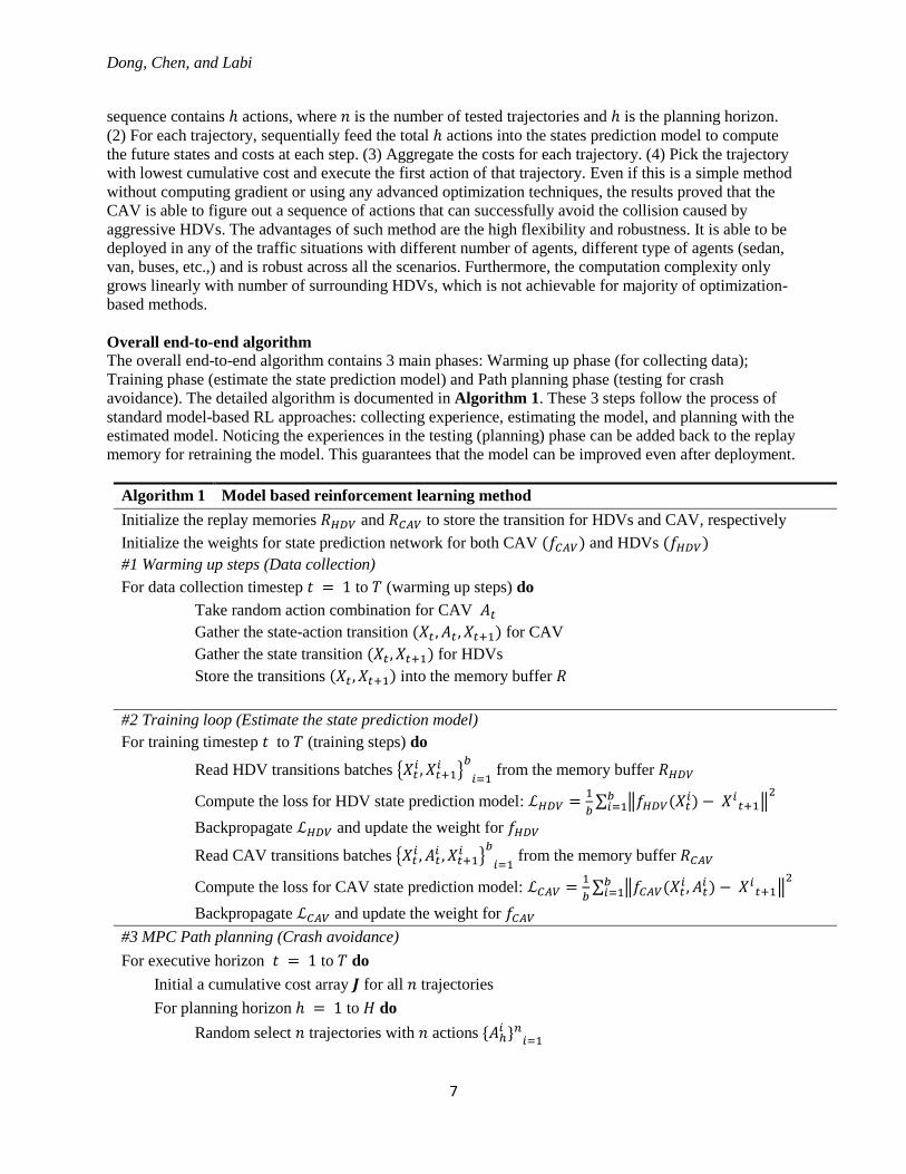
Overall end-to-end algorithm

The overall end-to-end algorithm contains 3 main phases: Warming up phase (for collecting data);

Training phase (estimate the state prediction model) and Path planning phase (testing for crash

avoidance). The detailed algorithm is documented in Algorithm 1. These 3 steps follow the process of

standard model-based RL approaches: collecting experience, estimating the model, and planning with the

estimated model. Noticing the experiences in the testing (planning) phase can be added back to the replay

memory for retraining the model. This guarantees that the model can be improved even after deployment.

Algorithm 1 Model based reinforcement learning method

Initialize the replay memories 𝑅𝐻𝐷𝑉 and 𝑅𝐶𝐴𝑉 to store the transition for HDVs and CAV, respectively

Initialize the weights for state prediction network for both CAV (𝑓𝐶𝐴𝑉) and HDVs (𝑓𝐻𝐷𝑉)

#1 Warming up steps (Data collection)

For data collection timestep 𝑡 = 1 to 𝑇 (warming up steps) do

Take random action combination for CAV 𝐴𝑡

Gather the state-action transition (𝑋𝑡 , 𝐴𝑡 , 𝑋𝑡+1) for CAV

Gather the state transition (𝑋𝑡 , 𝑋𝑡+1) for HDVs

Store the transitions (𝑋𝑡 , 𝑋𝑡+1) into the memory buffer 𝑅

#2 Training loop (Estimate the state prediction model)

For training timestep 𝑡 to 𝑇 (training steps) do

Read HDV transitions batches {𝑋𝑡𝑖 , 𝑋𝑡+1

𝑖 }𝑏

𝑖=1 from the memory buffer 𝑅𝐻𝐷𝑉

Compute the loss for HDV state prediction model: ℒ𝐻𝐷𝑉 =1

𝑏∑ ‖𝑓𝐻𝐷𝑉(𝑋𝑡

𝑖) − 𝑋𝑖𝑡+1‖

2𝑏𝑖=1

Backpropagate ℒ𝐻𝐷𝑉 and update the weight for 𝑓𝐻𝐷𝑉

Read CAV transitions batches {𝑋𝑡𝑖 , 𝐴𝑡

𝑖 , 𝑋𝑡+1𝑖 }

𝑏

𝑖=1 from the memory buffer 𝑅𝐶𝐴𝑉

Compute the loss for CAV state prediction model: ℒ𝐶𝐴𝑉 =1

𝑏∑ ‖𝑓𝐶𝐴𝑉(𝑋𝑡

𝑖, 𝐴𝑡𝑖 ) − 𝑋𝑖

𝑡+1‖2𝑏

𝑖=1

Backpropagate ℒ𝐶𝐴𝑉 and update the weight for 𝑓𝐶𝐴𝑉

#3 MPC Path planning (Crash avoidance)

For executive horizon 𝑡 = 1 to 𝑇 do

Initial a cumulative cost array 𝑱 for all 𝑛 trajectories

For planning horizon ℎ = 1 to 𝐻 do

Random select 𝑛 trajectories with 𝑛 actions {𝐴ℎ𝑖 }𝑛

𝑖=1


8

For each action 𝐴ℎ𝑖 in 𝑛 trajectories do

Predict the future states for ego CAV: ��𝐶𝐴𝑉ℎ+1 = 𝑓𝐶𝐴𝑉(𝑋ℎ, 𝐴ℎ

𝑖 )

Predict the future states all surrounding HDVs: ��𝐻𝐷𝑉ℎ+1 = 𝑓𝐻𝐷𝑉(𝑋ℎ)

Compute the TTC based cost for each trajectory using Equation (6)

Update the cumulative cost for each trajectory and saved in 𝑱

Pick the trajectories with lowest cumulative cost: 𝑖∗ = 𝑎𝑟𝑔𝑚𝑖𝑛(𝑱)

Execute the first action of 𝐴1𝑖∗

Add (𝑋𝑡𝐶𝐴𝑉 , 𝐴1

𝑖∗ , 𝑋𝑡+1𝐶𝐴𝑉) into 𝑅𝐶𝐴𝑉, (𝑋𝑡

𝐻𝐷𝑉 , 𝑋𝑡+1𝐻𝐷𝑉)

EXPERIMENT SETTINGS

Scenario settings

Among many crash imminent situations caused by the human drivers faults, the 2 cases (rear end and side

impact) shown in Figure 1 are most frequent (27) . These 2 situations are mainly originated from the

illegal or aggressive lane changings from the grey-colored vehicles in the figure. This can happen in the

real world when the red-colored vehicle is in the blind spot of the grey-colored vehicle.

(a) rear end impact (b) side impact

Figure 1. collision patterns (red: CAV, grey: HDV)

Figure 2. Simulated situation in CARLA

To establish this most-frequent safety-imminent case in the CARLA simulator, we introduce 4

vehicles as shown in the Figure 2, the yellow vehicle represents the “at fault” HDV and the CAV is in

red. This setting can be described as follows: the yellow HDV wish to overtake the grey vehicle but fail to

identify the red vehicle (CAV) in its blind spot. This aggressive lane changing will likely to cause a crash

particularly where the driving environment is compact (the CAV cannot brake hard since this will cause

the rear end collision with the blue HDV). This would require the CAV to generate a sequence of

maneuver to avoid the crash under this imminent situation. Note that in the simulation, other than the


9

cases shown in Figure 2, we also establish scenarios for yellow HDV to overtake from left and may cause

a side-swipe collision with CAV on the right. This extra setting is to test the robustness of the model. The

simulation step size is set as 0.05s/step (or 20 steps/s), and the aggressive overtaking maneuver for yellow

HDV is generated manually by driving the vehicle with Logitech G27 Racing Wheel. To facilitate the RL

experiments, we further develop a Open AI gym (25) interface with the Python API to connect CARLA

simulator.

State space

The state describes the driving environment for both CAV and surrounding HDVs is the input fed into the

trajectory prediction model to get the future states. For the state space in this research, we consider the

historical location, speed, acceleration in both 𝑥 and 𝑦 directions for ego-CAV and surrounding vehicles

in the past 𝑛 timesteps. Moreover, for ego-CAV, since the control commands are available, it should be

included into the state for better state prediction. The state for HDVs and CAV are as follows:

𝑋𝐻𝐷𝑉 = [

𝑥1 𝑦1 𝑣𝑥1 𝑣𝑦1 𝑎𝑥1 𝑎𝑦1

⋮ ⋮ ⋮ ⋮ ⋮ ⋮𝑥𝑛 𝑦𝑛 … … 𝑎𝑥𝑛 𝑎𝑦𝑛

]

𝑛×6

(6)

[𝑋𝐶𝐴𝑉 , 𝐴𝐶𝐴𝑉] = [

𝑥1 𝑦1 𝑣𝑥1 𝑣𝑦1 𝑎𝑥1 𝑎𝑦1 𝑡ℎ𝑟𝑜𝑡𝑡𝑙𝑒1 𝑠𝑡𝑒𝑒𝑟𝑖𝑛𝑔1 𝑏𝑟𝑒𝑎𝑘1

⋮ ⋮ ⋮ ⋮ ⋮ ⋮ ⋮ ⋮ ⋮𝑥𝑛 𝑦𝑛 … … 𝑎𝑥𝑛 𝑎𝑦𝑛 𝑡ℎ𝑟𝑜𝑡𝑡𝑙𝑒𝑛 𝑠𝑡𝑒𝑒𝑟𝑖𝑛𝑔𝑛 𝑏𝑟𝑒𝑎𝑘𝑛

]

𝑛×6

(7)

In this work, we set the history window size 𝑛 = 5.

Action space

As the control commands (throttle, brake pedal position and steering angle) are all continuous variables

that can take infinite number of values, it is difficult to efficiently search such infinite action space. Also,

some control commands should be constrained. For example, the steering angle should be constrained by

“inertia”, meaning the consecutive commands should be close since it is unsafe to make drastic changes

within a short period of time. Also, the brake and gas pedal should be exclusive and cannot be pressed

simultaneously. To reduce the action space and consider these interval constraints, we discretize the

action space to make them discrete variable and use a fixed transfer logic to map the discretized variable

back to original control commands. Specifically, we define 2 categorical variables for longitudinal control

and latitudinal control, respectively. Each variable can take value from set {0, 1, 2}, The first variable

determines whether current action should be gas, brake, or nothing (keep). For the steering angle, the

categorical variable determines the incremental direction (left, right, or keep) of the steer wheel.

Therefore, if the latitudinal control command is not zero, the steering will either subtract (turn left) 0.1

unit (this unit is defined by the simulator, the total range of the steering angle is -1 to 1 while -1 is the full

left and 1 the full right) or add 0.1 unit (turn right) based on the current steering position. Under this

setting, we shrink the overall action space to 3 × 3 = 9 actions, which can be easily searched.

𝑙𝑜𝑛𝑔𝑖𝑡𝑢𝑑𝑖𝑛𝑎𝑙 = {0 𝑏𝑟𝑎𝑘𝑒1 𝑘𝑒𝑒𝑝2 𝑔𝑎𝑠

(8)

𝑙𝑎𝑡𝑖𝑡𝑢𝑑𝑖𝑛𝑎𝑙 = {

0 𝑙𝑒𝑓𝑡1 𝑘𝑒𝑒𝑝2 𝑟𝑖𝑔ℎ𝑡

(9)


10

RESULTS

State prediction model

Figure 3 shows the training curves of all the three state prediction models for both CAV and HDVs. The

loss is the mean squared error between the predicted state and ground truth state captured from actual

trajectories. The models converge very fast after several epochs while the linear regression (linreg) model

has the best prediction performance and convergence rate. The result indicates even with the easiest

model linear regression, the prediction accuracy can be guaranteed, and it can even outperform other

neural networks. The reason is that for the imminent situations in Figure 2, The timestep size is small

(0.05s/step), thus all the vehicles have limited maneuvers that can be easily captured with a simple model.

It worth noting that linear regression model converges so fast that can even be trained online after

collecting trajectories for surrounding vehicles in the real-world deployment phase. This property

facilitates the high robustness for the algorithm since it can always “learn” right away when facing new

situations.

(a) HDV state prediction (b) CAV state prediction

Figure 3. Training curves for both state prediction model

Figure 4 shows the example of location prediction for both CAV and HDV in 5 random

trajectories for the single-layered neural network (linear regression). The dash line in the figure represents

the input trajectory (location in the past 𝑛 steps), the dot represents the location of the ground truth (label)

and the star location is the predicted location. It is obvious that the CAV state prediction model has

superior performance because the stars and dots have more coinciding cases. Also, the errors in the

location prediction is comparatively low (lower than 1 meter), which we can be handled by the MPC

based planning method.

Figure 4. Example location prediction in both x and y directions (Linear regression model)


11

Success rate

The test cases we created are non-trivial so that there will be 100% crash if no proper evasive decisions

maneuvers are executed. We adopt, as the main evaluation metric, the success rate for crash avoidance

after CAV executes all the planned actions and fully stops. Since the linear regression model has the best

performance in the state prediction, we test the proposed crash avoidance system built with this model

under several multiple critical scenarios with different initial average speed: 15m/s, 20m/s, 25m/s; and

different combinations of model parameters: number of random trajectories 𝑛 = 5, 10, 20, 30 vs. planning

horizons ℎ = 1, 3, 5,7,10. Here, the average speed is the mean initial speed of all 4 vehicles, for each

testing round, a random normal noise with zero mean and a standard deviation of 1𝑚/𝑠 is added to each

vehicle. This is to guarantee the heterogeneity of the driving environment. Generally, the scenarios with

higher initial average speed are riskier and have higher chance of collision. Each setting is tested 20

times, the average success rates of avoiding the crash vs. the model parameters are shown in Figure 5.

(a) 15 m/s (b) 20 m/s (c) 25 m/s

Figure 5. Success rate for avoiding the crashes with different initial average speed

From the Figure 5, it is obvious that the model parameters (number of trajectories and planning

horizion) can greatly affect the avoidance rate. An increase in the number of trajectories can generally

enhance the performance because more trials with more future possibilities can be evaluated. However,

more trajectories means more computation is needed. With regard to the planning horizons, from the

results above, it can be observed that either too large or too small planning horizon can harm the model

performance in terms of the success rate. The optimal planning horizon is 3 steps (0.15s). The reason is

that all the scenarios belong to crash-imminent situations, planning long into the future can be of no use

because the crash will happen within a short period. Also, since the prediction error caused by

discrepancies between the predicted trajectories and the actual trajectories driven by both HDVs and CAV

is inevitable, longer planning horizon can induce larger drift. Furthermore, after testing multiple rounds,

the experiences can be saved to further train the state prediction model. This property facilitates the

improvement of the framework even after deployment.

CONCLUDING REMARKS

In this research, we developed a simple, fast model-based reinforcement learning framework for CAV to

avoid collision caused by the external human error. The framework contains 2 cooperative submodules

(state prediction and path planning) that can be trained end-to-end and has the capability of being

improved online after deployment. The framework is a data-driven approach that does not require any

prior knowledge or assumptions on the vehicle dynamics or physical models, but also has benefits of data

efficiency from conventional planning-based method. Therefore, the flexibility and robustness can be

expected under various of safety imminent situations with different vehicle number and types (i.e., truck

or bus). After being deployed and tested in the CARLA environment, the results demonstrate the

proposed algorithm can reach a high success rate of crash avoidance at least 85% even in a highly

compact driving environments which have 100% crash rate if without proper evasive maneuver.


12

Moving forward, the framework can be tested by incorporating more testing scenarios containing

different crash patterns other than side-impact. Also with vehicle connectivity (28–30), cooperative

maneuvers can be expected to have higher performance particularly in the compact and complicated

driving environments (31–35). In other words, the CAV can take over the control for surrounding CHDVs

to make collaborative decisions to avoid a crash. Therefore, the cooperative maneuver with more than 1

agent and large action space can be further investigated in future research.

ACKNOWLEDGMENTS

This work was supported by Purdue University’s Center for Connected and Automated Transportation

(CCAT), a part of the larger CCAT consortium, a USDOT Region 5 University Transportation Center

funded by the U.S. Department of Transportation, Award #69A3551747105. The map data is from

OpenStreetMap contributors and is available from https://www.openstreetmap.org. The contents of this

paper reflect the views of the authors, who are responsible for the facts and the accuracy of the data

presented herein, and do not necessarily reflect the official views or policies of the sponsoring

organization. This manuscript is herein submitted for PRESENTATION ONLY at the 2022 Annual

Meeting of the Transportation Research Board.

AUTHOR CONTRIBUTIONS The authors confirm contribution to the paper as follows: all authors contributed to all sections. All

authors reviewed the results and approved the final version of the manuscript.

https://www.openstreetmap.org/

REFERENCES

1. World Health Organization. The Global Status Report on Road Safety 2018. 2018.

2. Lagarde, E. Road Traffic Injuries. In Encyclopedia of Environmental Health.

3. Rahman, M. S., M. Abdel-Aty, J. Lee, and M. H. Rahman. Safety Benefits of Arterials’ Crash

Risk under Connected and Automated Vehicles. Transportation Research Part C: Emerging

Technologies, 2019. https://doi.org/10.1016/j.trc.2019.01.029.

4. Noy, I. Y., D. Shinar, and W. J. Horrey. Automated Driving: Safety Blind Spots. Safety Science.

5. Ye, L., and T. Yamamoto. Evaluating the Impact of Connected and Autonomous Vehicles on

Traffic Safety. Physica A: Statistical Mechanics and its Applications, 2019.

https://doi.org/10.1016/j.physa.2019.04.245.

6. Ha, P., S. Chen, R. Du, J. Dong, Y. Li, and S. Labi. Vehicle Connectivity and Automation: A

Sibling Relationship. Frontiers in Built Environment.

7. Zwetsloot, G. I. J. M., M. Aaltonen, J. L. Wybo, J. Saari, P. Kines, and R. Op De Beeck. The Case

for Research into the Zero Accident Vision. Safety Science.

8. Kalra, N., and S. M. Paddock. Driving to Safety: How Many Miles of Driving Would It Take to

Demonstrate Autonomous Vehicle Reliability? Transportation Research Part A: Policy and

Practice, 2016. https://doi.org/10.1016/j.tra.2016.09.010.

9. Koopman, P., and M. Wagner. Autonomous Vehicle Safety: An Interdisciplinary Challenge. IEEE

Intelligent Transportation Systems Magazine, 2017. https://doi.org/10.1109/MITS.2016.2583491.

10. Naranjo, J. E., C. González, R. García, and T. De Pedro. Lane-Change Fuzzy Control in

Autonomous Vehicles for the Overtaking Maneuver. IEEE Transactions on Intelligent

Transportation Systems, 2008. https://doi.org/10.1109/TITS.2008.922880.

11. Feng, S., X. Yan, H. Sun, Y. Feng, and H. X. Liu. Intelligent Driving Intelligence Test for

Autonomous Vehicles with Naturalistic and Adversarial Environment. Nature Communications,

2021. https://doi.org/10.1038/s41467-021-21007-8.

12. Dosovitskiy, A., G. Ros, F. Codevilla, A. López, and V. Koltun. CARLA: An Open Urban Driving

Simulator. Proceedings of the 1st Annual Conference on Robot Learning.

13. Cai, P., Y. Lee, Y. Luo, and D. Hsu. SUMMIT: A Simulator for Urban Driving in Massive Mixed

Traffic. 2020.

14. Moerland, T. M., J. Broekens, and C. M. Jonker. Model-Based Reinforcement Learning: A

Survey. Proceedings of the International Conference on Electronic Business (ICEB), 2020.

15. Bertsekas, D. P. Dynamic Programming and Optimal Control. 2012.

16. Sutton, R. S., and A. G. Barto. Reinforcement Learning : An Introduction 2nd (19 June, 2017).

Neural Networks IEEE Transactions on, 2017.

17. Houenou, A., P. Bonnifait, V. Cherfaoui, and W. Yao. Vehicle Trajectory Prediction Based on

Motion Model and Maneuver Recognition. 2013.

18. Lefèvre, S., D. Vasquez, and C. Laugier. A Survey on Motion Prediction and Risk Assessment for

Intelligent Vehicles. ROBOMECH Journal.

19. Deo, N., and M. M. Trivedi. Convolutional Social Pooling for Vehicle Trajectory Prediction.

2018.

20. Bahari, M., I. Nejjar, and A. Alahi. Injecting Knowledge in Data-Driven Vehicle Trajectory

Predictors. Transportation Research Part C: Emerging Technologies, 2021.

https://doi.org/10.1016/j.trc.2021.103010.

21. Werling, M., and D. Liccardo. Automatic Collision Avoidance Using Model-Predictive Online

Optimization. 2012.

22. Shen, C., H. Guo, F. Liu, and H. Chen. MPC-Based Path Tracking Controller Design for

Autonomous Ground Vehicles. 2017.

23. Wang, H., Y. Huang, A. Khajepour, Y. Zhang, Y. Rasekhipour, and D. Cao. Crash Mitigation in

Motion Planning for Autonomous Vehicles. IEEE Transactions on Intelligent Transportation

Systems, 2019. https://doi.org/10.1109/TITS.2018.2873921.

24. Babu, M., R. R. Theerthala, A. K. Singh, B. P. Baladhurgesh, B. Gopalakrishnan, K. M. Krishna,


14

and S. Medasani. Model Predictive Control for Autonomous Driving Considering Actuator

Dynamics. 2019.

25. Brockman, G., V. Cheung, L. Pettersson, J. Schneider, J. Schulman, J. Tang, and W. Zaremba.

OpenAI Gym. 2016, pp. 1–4.

26. Nadimi, N., D. R. Ragland, and A. Mohammadian Amiri. An Evaluation of Time-to-Collision as a

Surrogate Safety Measure and a Proposal of a New Method for Its Application in Safety Analysis.

Transportation Letters, 2020. https://doi.org/10.1080/19427867.2019.1650430.

27. Xu, C., Z. Ding, C. Wang, and Z. Li. Statistical Analysis of the Patterns and Characteristics of

Connected and Autonomous Vehicle Involved Crashes. Journal of Safety Research, 2019.

https://doi.org/10.1016/j.jsr.2019.09.001.

28. Chen, S., Dong, J., Ha, P., Li, Y., Labi, S. Graph neural network and reinforcement learning for

multi-agent cooperative control of connected autonomous vehicles. Computer-Aided Civil and

Infrastructure Engineering, 2021. 36(7), 838-857.

29. Chen, S., Y. Leng, and S. Labi. A Deep Learning Algorithm for Simulating Autonomous Driving

Considering Prior Knowledge and Temporal Information. Computer-Aided Civil and

Infrastructure Engineering, 2019. https://doi.org/10.1111/mice.12495.

30. Dong, J., Chen, S., Y. Li, R. Du, A. Steinfeld, and S. Labi. Space-Weighted Information Fusion

Using Deep Reinforcement Learning: The Context of Tactical Control of Lane-Changing

Autonomous Vehicles and Connectivity Range Assessment. Transportation Research Part C:

Emerging Technologies, 2021. https://doi.org/10.1016/j.trc.2021.103192.

31. Du, R., Chen, S., Li, Y., Ha, P., Dong, J., Labi, S., Anastasopoulos, PC. (2021). A cooperative

crash avoidance framework for autonomous vehicle under collision-imminent situations in mixed

traffic stream. IEEE Intelligent Transportation Systems Conference (ITSC), September 19-22,

2021. Indianapolis, IN, United States.

32. Dong, J., Chen, S., Zong, S., Chen, T., Labi, S. (2021). Image transformer for explainable

autonomous driving system. IEEE Intelligent Transportation Systems Conference (ITSC),

September 19-22, 2021. Indianapolis, IN, United States.

33. Du, R., Chen, S., Dong, J., Ha, P., Labi, S. (2021). GAQ-EBkSP: A DRL-based Urban Traffic

Dynamic Rerouting Framework using Fog-Cloud Architecture. IEEE International Smart Cities

Conference (ISC2), September 7-10, 2021 – Virtual Conference.

34. Dong, J., Chen, S., Li, Y., Du, R., Steinfeld, A., Labi, S. (2020). Spatio-weighted information

fusion and DRL-based control for connected autonomous vehicles. IEEE Intelligent

Transportation Systems Conference (ITSC), September 20 – 23, 2020. Rhodes, Greece.

35. Ha, P., Chen, S., Du, R., Dong, J., Li, Y., Labi, S. (2020). Vehicle connectivity and automation: a

sibling relationship. Frontiers in Built Environment, 6, 199.

addressing crash-imminent situations caused by human

Documents