additive main effects and multiplicative interaction
TRANSCRIPT
Additive main effects and multiplicative interaction analysesof yield performance in rice genotypes for generaland specific adaptation to salt stress in locations in India
S. L. Krishnamurthy . P. C. Sharma . D. K. Sharma . Y. P. Singh .
V. K. Mishra . D. Burman . B. Maji . S. Mandal . S. K. Sarangi .
R. K. Gautam . P. K. Singh . K. K. Manohara . B. C. Marandi .
K. Chattopadhyay . G. Padmavathi . P. B. Vanve . K. D. Patil .
S. Thirumeni . O. P. Verma . A. H. Khan . S. Tiwari . S. Geetha .
R. Gill . V. K. Yadav . B. Roy . M. Prakash . A. Anandan . J. Bonifacio .
A. M. Ismail . R. K. Singh
Received: 25 December 2019 / Accepted: 18 November 2020 / Published online: 19 January 2021
� The Author(s) 2021
Abstract The aim of this study was to identify
stable rice genotypes tolerant to a salt stress environ-
ment and to identify ideal mega-environments using
AMMI (additive main effects and multiplicative
interaction) stability model analysis. A total of 13
rice genotypes and three salt tolerance checks were
evaluated across 13 salt stress locations (alkaline and
saline) for the two kharif seasons of 2014 and 2015.
Genotype CSR 36 (CHK3) was found to be the most
ideal of those tested. Genotypes CHK2 (CST 27) and
IR 87952-1-1-1-2-3-B (G05) were found to be the
most stable, with above average yields. The check
CSR 36 (CHK3) genotype was the best performer in
the majority of the environments studied, followed by
S. L. Krishnamurthy (&) � P. C. Sharma (&) �D. K. Sharma
Central Soil Salinity Research Institute, Karnal, India
e-mail: [email protected]
P. C. Sharma
e-mail: [email protected]
Y. P. Singh � V. K. Mishra
Central Soil Salinity Research Institute, Regional
Research Station, Lucknow, India
D. Burman � B. Maji � S. Mandal � S. K. Sarangi
Central Soil Salinity Research Institute, Regional
Research Station, Canning Town, India
R. K. Gautam � P. K. Singh
Central Island Agricultural Research Institute, Port Blair,
Andaman and Nicobar Islands, India
K. K. Manohara
Central Coastal Agricultural Research Institute (CCARI),
Old Goa (Ela), Goa, India
B. C. Marandi � K. Chattopadhyay � A. Anandan
National Rice Research Institute (NRRI), Cuttack,
Odisha, India
G. Padmavathi
Indian Institute of Rice Research, Hyderabad,
Telengana, India
P. B. Vanve � K. D. Patil
Khar Land Research Station, Dr. Balasaheb Sawant
Konkan Krishi Vidyapeeth Agricultural University,
Panvel, Maharashtra, India
S. Thirumeni
Pandit Jawaharlal Nehru College of Agriculture and
Research Institute, Karaikal, Puducherry, India
O. P. Verma � A. H. Khan
Narendra Deva University of Agriculture and Technology,
Faizabad, Uttar Pradesh, India
S. Tiwari
Rajendra Prasad Central Agricultural University,
Samastipur, Bihar, India
123
Euphytica (2021) 217:20
https://doi.org/10.1007/s10681-020-02730-7(0123456789().,-volV)( 0123456789().,-volV)
CSR 27 (CHK2) and IR 87952-1-1-1-2-3-B (G05)
which were the best genotypes in the mega-environ-
ment consisting of 21 environments evaluated across
stress locations and year combinations. Overall, the
most promising genotype (IR 87952-1-1-1-2-3-B) had
high mean yield and stability and could be used for
commercial cultivation or used as donor for breeding
programs across salt-affected soils. The genotypes
GN13 (IR 87938-1-1-2-1-3-B) and GN11 (IR
87938-1-2-2-1-3-B) showed 60–80% yield advantage
at specific salt stress locations, showing that these
genotypes could be used for specific environments of
salt-affected soils in India.
Keywords Salt � Rice � Additive main effects and
multiplicative interaction (AMMI) model � Mega-
environment
Introduction
Soil salinity is adversely affecting agricultural pro-
ductivity in approximately 900 million ha worldwide
(FAO 2014). In India, 6.73 million ha are current
affected by salt degradation, with the extent of salt-
affected areas predicted to increase due to the
repercussions of climate change, thereby threatening
future food security (Mondal et al. 2009). With
increasing temperature, the low-lying coastal areas
will be inundated more frequently by the sea water,
exposing yet more land to salinity. In inland areas, salt
accumulation is becoming an increasing challenging
to crop production due to the build-up of salts and
interactions with temperature as a consequence of
improper drainage and the use of poor-quality irriga-
tion water, particularly in arid and semiarid regions
(Munns and Tester 2008; Tack et al. 2015). Conse-
quent, the need to address this problem is urgent. The
deployment of salt-tolerant crop varieties is the most
effective, economic and environmentally friendly
approach. Rice is inherently a salt-sensitive crop, with
an electrical conductivity of soil-saturated extract
(ECe) of 3 dS m-1 being considered as the salinity
tolerance threshold for rice (Mohammadi et al. 2013).
In terms of limiting rice production, soil salinity is
considered to be a major abiotic stress, after drought,
limiting rice production in about 30% of rice growing
areas (Wu and Garg 2003). The differential response
of different rice genotypes to salinity and alkalinity at
different growth stages and the lack of correlation
between these responses (Krishnamurthy et al. 2016c),
low selection efficiency of agronomic characters, lack
of effective evaluation methods for salt tolerance
among genotypes and the complexity of salinity
tolerance phenotypes among genotypes are all factors
impeding rice breeding programs for salt tolerance
(Singh and Flowers 2010). Despite these challenges,
several salt-tolerant rice varieties have been released
in India and other rice-producing countries.
In addition to variable salinity levels, location-
specific weather conditions also contribute signifi-
cantly to genotype 9 environmental (G 9 E) interac-
tion, with the result that identifying tolerant and
stable genotypes is tricky. The intensity of salinity
stress may increase with higher temperature, thereby
effecting more grain yield loss in rice (Tack et al.
2015). Rice is most sensitive to salt stress at the early
seedling and reproductive growth stages. Grain yield
and salinity are governed by polygenic traits, and the
effect of environment is more pronounced in poly-
genic traits than monogenic ones. Hence, analysis of
such polygenic traits for salt tolerance across different
locations is quite difficult. In order that meaningful
conclusions can be drawn, a robust statistical analysis
is required when genotypes are evaluated under
different levels of salt stress at multiple locations
S. Geetha
Anbil Dharmalingam Agricultural College and Research
Institute, Trichy, Tamil Nadu, India
R. Gill
Punjab Agricultural University, Ludhiana,
Punjab, India
V. K. Yadav
Chandra Shekhar Azad University of Agriculture and
Technology, Kanpur, Uttar Pradesh, India
B. Roy
Centre for Strategic Studies, Salt Lake City,
Kolkata , India
M. Prakash
Annamalai University, Chidambaram,
Tamil Nadu, India
J. Bonifacio � A. M. Ismail � R. K. Singh (&)
International Rice Research Institute, Los Banos,
Philippines
e-mail: [email protected]
123
20 Page 2 of 15 Euphytica (2021) 217:20
across seasons. An understanding of the nature and
causes of such genotype-by-environment interactions
(GEI) across locations affected by salinity will help us
to identify the genotype that is stable across the
different salt stress locations (Krishnamurthy et al.
2017).
Among all the statistical models propounded for
dealing with G 9 E data, the additive main effects and
multiplicative interactions (AMMI) model (Zobel
et al. 1988; Gauch 1992) and genotype main effect
plus genotype by environment (GGE) biplot analysis
(Yan et al. 2000) are the best fit to analyze such
intricate datasets. These two models are supported by
biplot (Gabriel 1971) visualizations that facilitate
interpretation of the data. There has been much
discussion and weighing of the advantages and
disadvantages of these two models in terms of
accuracy, reliability and superiority (Gauch 2006;
Yan et al. 2007; Gauch et al. 2008; Yang et al. 2009;
Yan and Holland 2010). According to Gauch (2006),
the AMMI model is a singular value decomposition
(SVD)-based statistical analysis that can be applied to
yield trial data in agricultural research for two reasons.
First, it offers a choice of model for visualizing data
and partitions the overall variation of agriculture
research into the main effects genotype (g in AMMI
model) and environment (e in AMMI model), as well
as the multiplication effect of GEI; consequently,
complex variations can be handled easily and sepa-
rately. Second, there is a prediction choice of model
family members for gaining predictive accuracy.
While AMMI and GGE are equivalent in terms of
efficacy, best practices require model diagnosis for
each individual dataset to determine which member is
the most predictively accurate. AMMI is always
superior or equal to GGE in this context, but best
practices of model diagnosis are needed to determine
which member family is the most predicative in terms
of accuracy. The best practice of AMMI involves (1)
analysis of variance (ANOVA), (2) model diagnosis,
(3) mega-environment delineation, and (4) agricul-
tural recommendations to exploit both broad and
narrow adaptation to increase yields (Gauch 2013).
Many earlier studies employed the AMMI stability
model to identify general and specific adaptation of
rice genotypes under salinity and alkaline stress
conditions in India and Bangladesh (Krishnamurthy
et al. 2015, 2016a, d; Islam et al. 2016) and in the
coastal regions of southern Bangladesh (Islam et al.
2016). However, these studies did not implement the
best practices of AMMI since they did not include
model diagnosis to increase the accuracy of the model
family. The G 9 E interaction coupled with the
complex nature of salinity is a challenge to rice
breeders as it complicates the testing and selection of
superior genotypes and, thereby, significantly reduces
progress in plant breeding.
Therefore, in the present study AMMI stability
analysis was utilized to handle data generated from a
multi-location trial (MLT) conducted across 13 salin-
ity stress locations in 2 years (2014, 2015). The aim of
the study was to identify superior test locations for the
screening of salt-tolerant rice genotypes; to isolate
stable rice genotypes with good yields for general and
specific adaptation to saline and alkaline stress loca-
tions; and to investigate the options of grouping salt-
tolerant locations so that mega-environment-specific
genotypes can be employed for the management of
soils affected by salinity.
Materials and methods
Plant materials and testing locations
The present investigation was conducted in 13 salt
stress locations across India, representing five saline
environments and eight alkaline environments, during
the wet seasons of 2014 and 2015. The description of
these locations is given in Table 1. The saline-
challenged soils of the chosen experimental locations
ranged from sandy loam to clay loam, with ECe
ranging from 3.2 to 11.0 dS m-1, while the alkaline-
challenged soils ranged from sandy loam to clay loam,
with pH ranging from 8.14 to 9.9. The ECe and pH
values given in Table 1 were measured prior to
transplanting, at the time of transplanting, at flowering
and at maturity, and subsequently averaged. Thirteen
putative salt-tolerant rice genotypes used in this study
were obtained from the International Rice Research
Institute (IRRI), Philippines, National Agricultural
Research and Extension System (NARES) partners
and Indian Council of Agricultural Research (ICAR)
institutes of India. They were evaluated across 13
locations during the kharif season of 2014 and 2015,
along with three checks, namely CST 7-1 (coastal
salinity), CSR 27 (inland salinity) and CSR 36
(alkalinity). Details on these genotypes are given in
123
Euphytica (2021) 217:20 Page 3 of 15 20
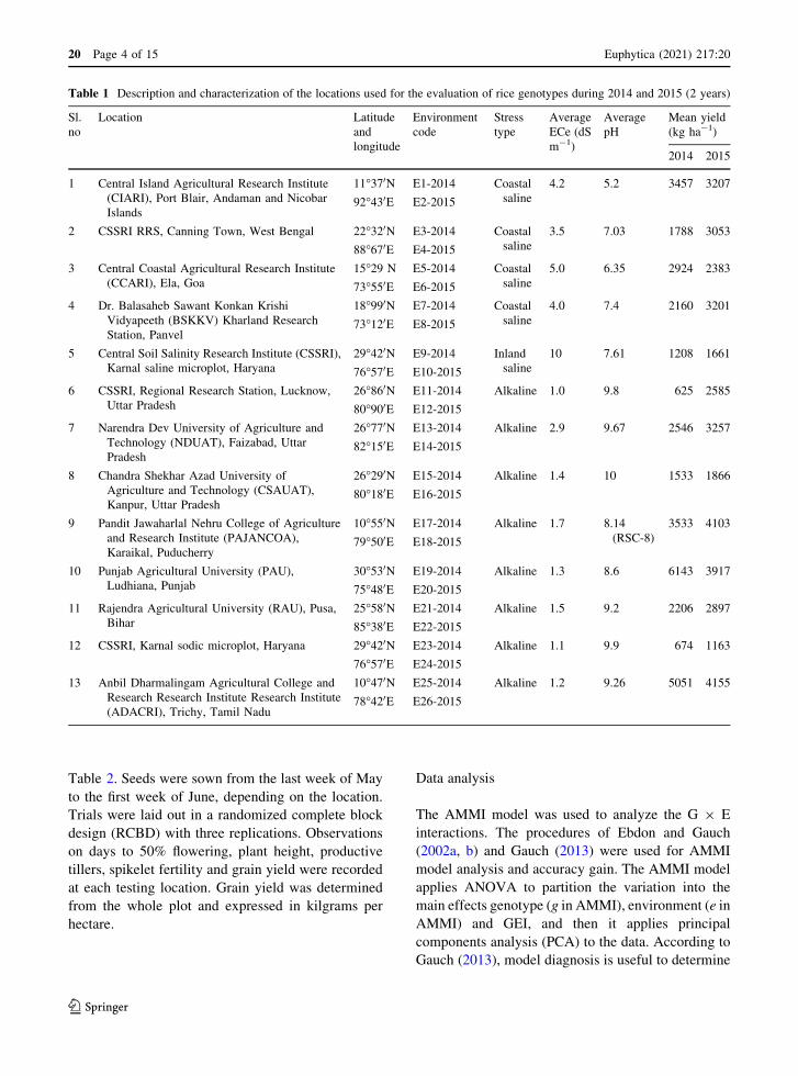
Table 2. Seeds were sown from the last week of May
to the first week of June, depending on the location.
Trials were laid out in a randomized complete block
design (RCBD) with three replications. Observations
on days to 50% flowering, plant height, productive
tillers, spikelet fertility and grain yield were recorded
at each testing location. Grain yield was determined
from the whole plot and expressed in kilgrams per
hectare.
Data analysis
The AMMI model was used to analyze the G 9 E
interactions. The procedures of Ebdon and Gauch
(2002a, b) and Gauch (2013) were used for AMMI
model analysis and accuracy gain. The AMMI model
applies ANOVA to partition the variation into the
main effects genotype (g in AMMI), environment (e in
AMMI) and GEI, and then it applies principal
components analysis (PCA) to the data. According to
Gauch (2013), model diagnosis is useful to determine
Table 1 Description and characterization of the locations used for the evaluation of rice genotypes during 2014 and 2015 (2 years)
Sl.
no
Location Latitude
and
longitude
Environment
code
Stress
type
Average
ECe (dS
m-1)
Average
pH
Mean yield
(kg ha-1)
2014 2015
1 Central Island Agricultural Research Institute
(CIARI), Port Blair, Andaman and Nicobar
Islands
11�370N E1-2014 Coastal
saline
4.2 5.2 3457 3207
92�430E E2-2015
2 CSSRI RRS, Canning Town, West Bengal 22�320N E3-2014 Coastal
saline
3.5 7.03 1788 3053
88�670E E4-2015
3 Central Coastal Agricultural Research Institute
(CCARI), Ela, Goa
15�29 N E5-2014 Coastal
saline
5.0 6.35 2924 2383
73�550E E6-2015
4 Dr. Balasaheb Sawant Konkan Krishi
Vidyapeeth (BSKKV) Kharland Research
Station, Panvel
18�990N E7-2014 Coastal
saline
4.0 7.4 2160 3201
73�120E E8-2015
5 Central Soil Salinity Research Institute (CSSRI),
Karnal saline microplot, Haryana
29�420N E9-2014 Inland
saline
10 7.61 1208 1661
76�570E E10-2015
6 CSSRI, Regional Research Station, Lucknow,
Uttar Pradesh
26�860N E11-2014 Alkaline 1.0 9.8 625 2585
80�900E E12-2015
7 Narendra Dev University of Agriculture and
Technology (NDUAT), Faizabad, Uttar
Pradesh
26�770N E13-2014 Alkaline 2.9 9.67 2546 3257
82�150E E14-2015
8 Chandra Shekhar Azad University of
Agriculture and Technology (CSAUAT),
Kanpur, Uttar Pradesh
26�290N E15-2014 Alkaline 1.4 10 1533 1866
80�180E E16-2015
9 Pandit Jawaharlal Nehru College of Agriculture
and Research Institute (PAJANCOA),
Karaikal, Puducherry
10�550N E17-2014 Alkaline 1.7 8.14
(RSC-8)
3533 4103
79�500E E18-2015
10 Punjab Agricultural University (PAU),
Ludhiana, Punjab
30�530N E19-2014 Alkaline 1.3 8.6 6143 3917
75�480E E20-2015
11 Rajendra Agricultural University (RAU), Pusa,
Bihar
25�580N E21-2014 Alkaline 1.5 9.2 2206 2897
85�380E E22-2015
12 CSSRI, Karnal sodic microplot, Haryana 29�420N E23-2014 Alkaline 1.1 9.9 674 1163
76�570E E24-2015
13 Anbil Dharmalingam Agricultural College and
Research Research Institute Research Institute
(ADACRI), Trichy, Tamil Nadu
10�470N E25-2014 Alkaline 1.2 9.26 5051 4155
78�420E E26-2015
123
20 Page 4 of 15 Euphytica (2021) 217:20
the best AMMI model family for a given dataset, and it
is advised to use the FR-test (Cornelius 1993) to assess
model diagnosis and to identify significant interaction
principal components (IPCs) in the AMMI model
using AMMISOFT software for the analysis of yield
trial data. AMMI constitutes a model family, with
AMMI0 having no IPC, AMMI1 having 1 IPC,
AMMI2 having 2 IPC, and so on up to AMMIF
(residual discarded). The AMMI model equation is:
Yge ¼ lþ ag þ be þ Rnkncgnden þ qge ð1Þ
where Yge is the yield of genotype g in environment e;
l is the grand mean; ag is the genotype deviation from
the grand mean; be is the environment deviation; kn is
the singular value for IPC n and correspondingly kn2 is
its eigenvalue; cgn is the eigenvector value for
genotype g and component n; den is the eigenvector
value for environment e and component n, with both
eigenvectors scaled as unit vectors; and qge is the
residual.
The interaction scores are commonly scaled as
kn0.5cgn and kn
0.5den so that their products estimate
interactions directly, without the need of yet another
multiplication by k.
The ratio of yield for AMMI ‘‘winners’’ within each
environment (identified in the first column of AMMI
ranks) was calculated by dividing the yield for the
overall winner (Gauch 2013). According to Gauch
(2013), a ratio of 1 represents a ‘‘winning’’ genotype
across environments. This ratio is an assessment of the
importance of narrow adaptation due to GEI effects,
with a ratio of C 1.10 indicative of narrow adaptation.
Results
ANOVA and identification of AMMI model
families
Analysis of variance for grain yield using the AMMI
model is presented in Table 3. Both the main effects
genotype (G), environment (E) and their interaction
(GEI) components were statistically significant at
p B 0.001) The environmental component explains
the largest proportion of variation (62.64%), followed
by G 9 E interaction components (approx. 27.98%
variation), with the genotypic component (G) explain-
ing the least variation (about 2.81% of the total
variation). The GEI effects were partitioned into seven
IPCs (IPC1–IPC7) and found to be significant at p B
0.01 for grain yield in different salt-affected environ-
ments across the year. In terms of contribution to the
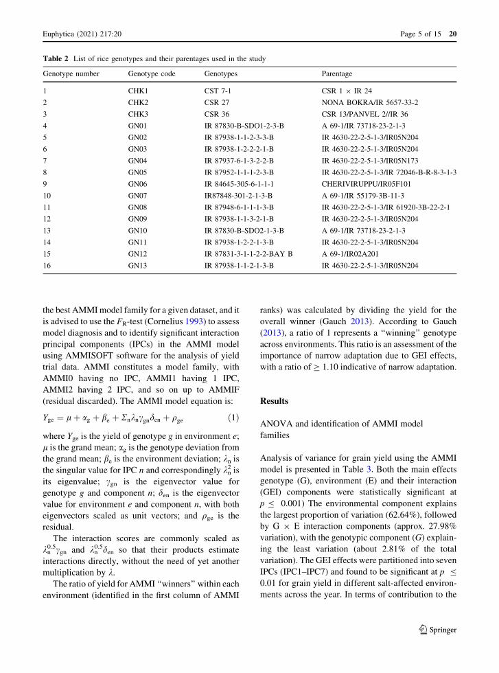
Table 2 List of rice genotypes and their parentages used in the study
Genotype number Genotype code Genotypes Parentage
1 CHK1 CST 7-1 CSR 1 9 IR 24
2 CHK2 CSR 27 NONA BOKRA/IR 5657-33-2
3 CHK3 CSR 36 CSR 13/PANVEL 2//IR 36
4 GN01 IR 87830-B-SDO1-2-3-B A 69-1/IR 73718-23-2-1-3
5 GN02 IR 87938-1-1-2-3-3-B IR 4630-22-2-5-1-3/IR05N204
6 GN03 IR 87938-1-2-2-2-1-B IR 4630-22-2-5-1-3/IR05N204
7 GN04 IR 87937-6-1-3-2-2-B IR 4630-22-2-5-1-3/IR05N173
8 GN05 IR 87952-1-1-1-2-3-B IR 4630-22-2-5-1-3/IR 72046-B-R-8-3-1-3
9 GN06 IR 84645-305-6-1-1-1 CHERIVIRUPPU/IR05F101
10 GN07 IR87848-301-2-1-3-B A 69-1/IR 55179-3B-11-3
11 GN08 IR 87948-6-1-1-1-3-B IR 4630-22-2-5-1-3/IR 61920-3B-22-2-1
12 GN09 IR 87938-1-1-3-2-1-B IR 4630-22-2-5-1-3/IR05N204
13 GN10 IR 87830-B-SDO2-1-3-B A 69-1/IR 73718-23-2-1-3
14 GN11 IR 87938-1-2-2-1-3-B IR 4630-22-2-5-1-3/IR05N204
15 GN12 IR 87831-3-1-1-2-2-BAY B A 69-1/IR02A201
16 GN13 IR 87938-1-1-2-1-3-B IR 4630-22-2-5-1-3/IR05N204
123
Euphytica (2021) 217:20 Page 5 of 15 20
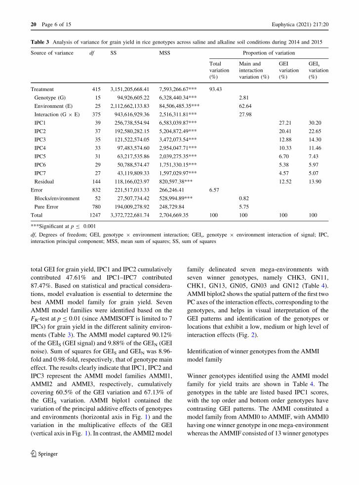
total GEI for grain yield, IPC1 and IPC2 cumulatively
contributed 47.61% and IPC1–IPC7 contributed
87.47%. Based on statistical and practical considera-
tions, model evaluation is essential to determine the
best AMMI model family for grain yield. Seven
AMMI model families were identified based on the
FR-test at p B 0.01 (since AMMISOFT is limited to 7
IPCs) for grain yield in the different salinity environ-
ments (Table 3). The AMMI model captured 90.12%
of the GEIS (GEI signal) and 9.88% of the GEIN (GEI
noise). Sum of squares for GEIS and GEIN was 8.96-
fold and 0.98-fold, respectively, that of genotype main
effect. The results clearly indicate that IPC1, IPC2 and
IPC3 represent the AMMI model families AMMI1,
AMMI2 and AMMI3, respectively, cumulatively
covering 60.5% of the GEI variation and 67.13% of
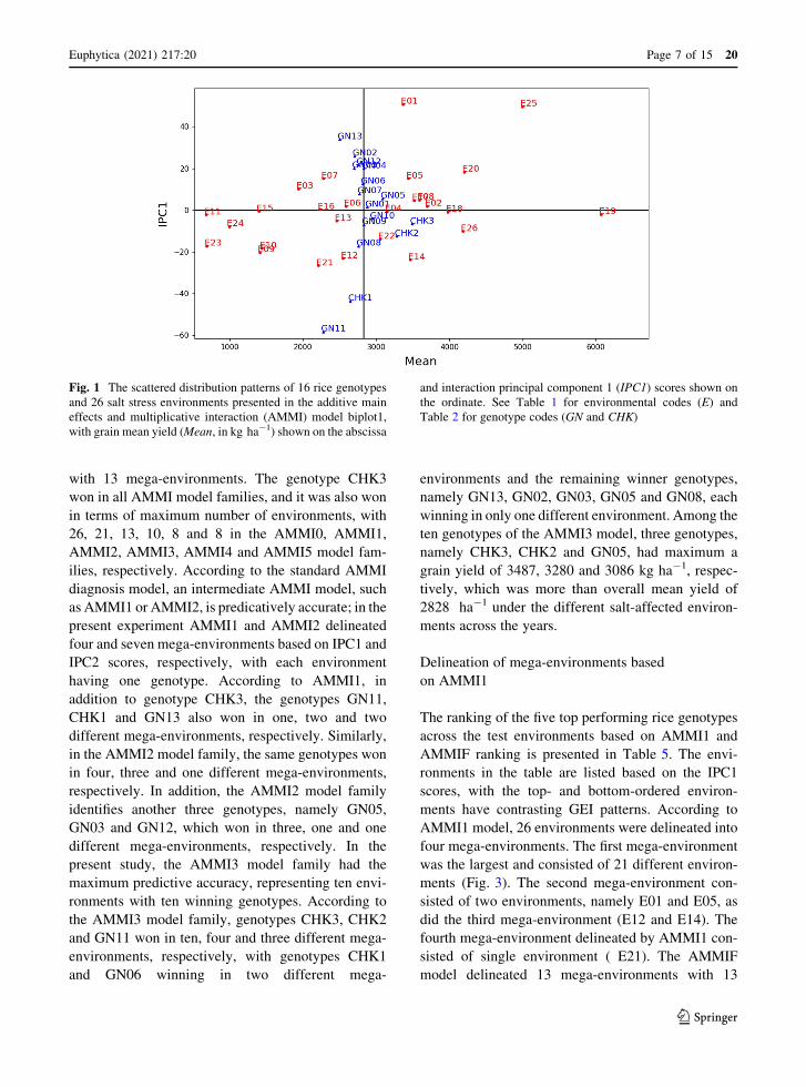
the GEIS variation. AMMI biplot1 contained the
variation of the principal additive effects of genotypes
and environments (horizontal axis in Fig. 1) and the
variation in the multiplicative effects of the GEI
(vertical axis in Fig. 1). In contrast, the AMMI2 model
family delineated seven mega-environments with
seven winner genotypes, namely CHK3, GN11,
CHK1, GN13, GN05, GN03 and GN12 (Table 4).
AMMI biplot2 shows the spatial pattern of the first two
PC axes of the interaction effects, corresponding to the
genotypes, and helps in visual interpretation of the
GEI patterns and identification of the genotypes or
locations that exhibit a low, medium or high level of
interaction effects (Fig. 2).
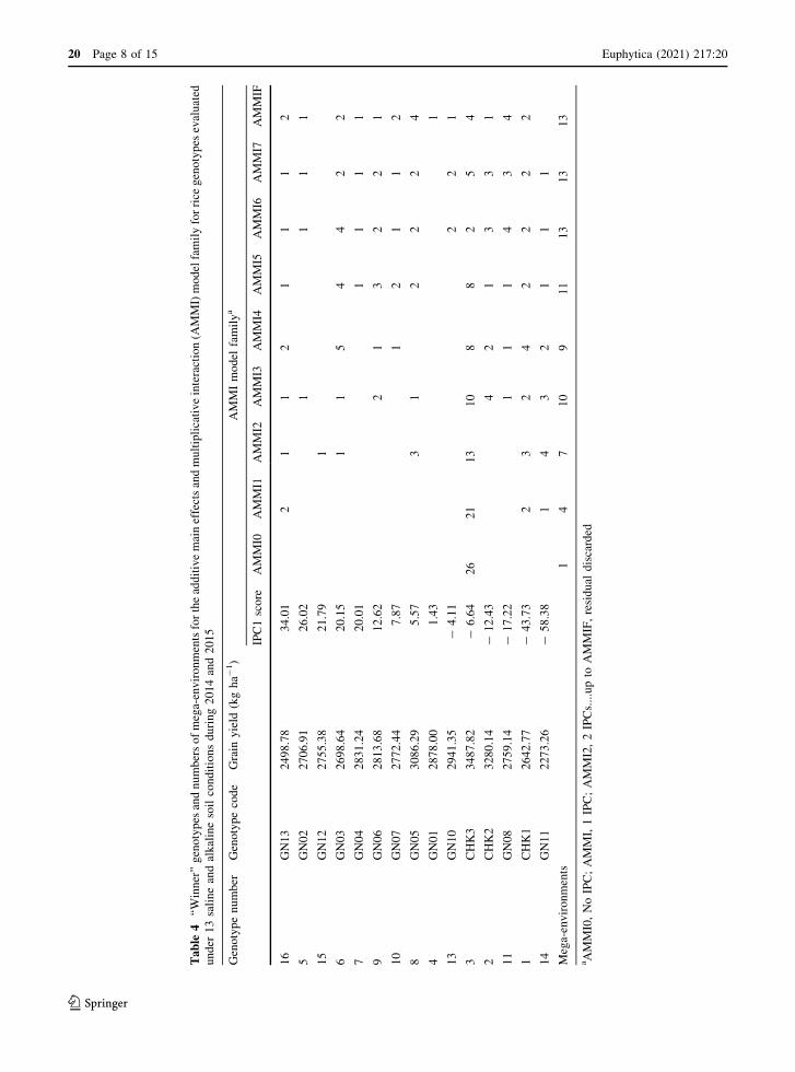
Identification of winner genotypes from the AMMI
model family
Winner genotypes identified using the AMMI model
family for yield traits are shown in Table 4. The
genotypes in the table are listed based IPC1 scores,
with the top order and bottom order genotypes have
contrasting GEI patterns. The AMMI constituted a
model family from AMMI0 to AMMIF, with AMMI0
having one winner genotype in one mega-environment
whereas the AMMIF consisted of 13 winner genotypes
Table 3 Analysis of variance for grain yield in rice genotypes across saline and alkaline soil conditions during 2014 and 2015
Source of variance df SS MSS Proportion of variation
Total
variation
(%)
Main and
interaction
variation (%)
GEI
variation
(%)
GEIs
variation
(%)
Treatment 415 3,151,205,668.41 7,593,266.67*** 93.43
Genotype (G) 15 94,926,605.22 6,328,440.34*** 2.81
Environment (E) 25 2,112,662,133.83 84,506,485.35*** 62.64
Interaction (G 9 E) 375 943,616,929.36 2,516,311.81*** 27.98
IPC1 39 256,738,554.94 6,583,039.87*** 27.21 30.20
IPC2 37 192,580,282.15 5,204,872.49*** 20.41 22.65
IPC3 35 121,522,574.05 3,472,073.54*** 12.88 14.30
IPC4 33 97,483,574.60 2,954,047.71*** 10.33 11.46
IPC5 31 63,217,535.86 2,039,275.35*** 6.70 7.43
IPC6 29 50,788,574.47 1,751,330.15*** 5.38 5.97
IPC7 27 43,119,809.33 1,597,029.97*** 4.57 5.07
Residual 144 118,166,023.97 820,597.38*** 12.52 13.90
Error 832 221,517,013.33 266,246.41 6.57
Blocks/environment 52 27,507,734.42 528,994.89*** 0.82
Pure Error 780 194,009,278.92 248,729.84 5.75
Total 1247 3,372,722,681.74 2,704,669.35 100 100 100 100
***Significant at p B 0.001
df, Degrees of freedom; GEI, genotype 9 environment interaction; GEIs, genotype 9 environment interaction of signal; IPC,
interaction principal component; MSS, mean sum of squares; SS, sum of squares
123
20 Page 6 of 15 Euphytica (2021) 217:20
with 13 mega-environments. The genotype CHK3
won in all AMMI model families, and it was also won
in terms of maximum number of environments, with
26, 21, 13, 10, 8 and 8 in the AMMI0, AMMI1,
AMMI2, AMMI3, AMMI4 and AMMI5 model fam-
ilies, respectively. According to the standard AMMI
diagnosis model, an intermediate AMMI model, such
as AMMI1 or AMMI2, is predicatively accurate; in the
present experiment AMMI1 and AMMI2 delineated
four and seven mega-environments based on IPC1 and
IPC2 scores, respectively, with each environment
having one genotype. According to AMMI1, in
addition to genotype CHK3, the genotypes GN11,
CHK1 and GN13 also won in one, two and two
different mega-environments, respectively. Similarly,
in the AMMI2 model family, the same genotypes won
in four, three and one different mega-environments,
respectively. In addition, the AMMI2 model family
identifies another three genotypes, namely GN05,
GN03 and GN12, which won in three, one and one
different mega-environments, respectively. In the
present study, the AMMI3 model family had the
maximum predictive accuracy, representing ten envi-
ronments with ten winning genotypes. According to
the AMMI3 model family, genotypes CHK3, CHK2
and GN11 won in ten, four and three different mega-
environments, respectively, with genotypes CHK1
and GN06 winning in two different mega-
environments and the remaining winner genotypes,
namely GN13, GN02, GN03, GN05 and GN08, each
winning in only one different environment. Among the
ten genotypes of the AMMI3 model, three genotypes,
namely CHK3, CHK2 and GN05, had maximum a
grain yield of 3487, 3280 and 3086 kg ha-1, respec-
tively, which was more than overall mean yield of
2828 ha-1 under the different salt-affected environ-
ments across the years.
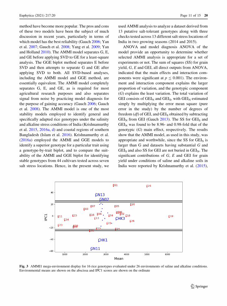
Delineation of mega-environments based
on AMMI1
The ranking of the five top performing rice genotypes
across the test environments based on AMMI1 and
AMMIF ranking is presented in Table 5. The envi-
ronments in the table are listed based on the IPC1
scores, with the top- and bottom-ordered environ-
ments have contrasting GEI patterns. According to
AMMI1 model, 26 environments were delineated into
four mega-environments. The first mega-environment
was the largest and consisted of 21 different environ-
ments (Fig. 3). The second mega-environment con-
sisted of two environments, namely E01 and E05, as
did the third mega-environment (E12 and E14). The
fourth mega-environment delineated by AMMI1 con-
sisted of single environment ( E21). The AMMIF
model delineated 13 mega-environments with 13
Fig. 1 The scattered distribution patterns of 16 rice genotypes
and 26 salt stress environments presented in the additive main
effects and multiplicative interaction (AMMI) model biplot1,
with grain mean yield (Mean, in kg ha-1) shown on the abscissa
and interaction principal component 1 (IPC1) scores shown on
the ordinate. See Table 1 for environmental codes (E) and
Table 2 for genotype codes (GN and CHK)
123
Euphytica (2021) 217:20 Page 7 of 15 20
Table
4‘‘
Win
ner
’’g
eno
typ
esan
dn
um
ber
so
fm
ega-
env
iro
nm
ents
for
the
add
itiv
em
ain
effe
cts
and
mu
ltip
lica
tiv
ein
tera
ctio
n(A
MM
I)m
od
elfa
mil
yfo
rri
ceg
eno
typ
esev
alu
ated
un
der
13
sali
ne
and
alk
alin
eso
ilco
nd
itio
ns
du
rin
g2
01
4an
d2
01
5
Gen
oty
pe
nu
mb
erG
eno
typ
eco
de
Gra
iny
ield
(kg
ha-
1)
AM
MI
mo
del
fam
ily
a
IPC
1sc
ore
AM
MI0
AM
MI1
AM
MI2
AM
MI3
AM
MI4
AM
MI5
AM
MI6
AM
MI7
AM
MIF
16
GN
13
24
98
.78
34
.01
21
12
11
12
5G
N0
22
70
6.9
12
6.0
21
11
1
15
GN
12
27
55
.38
21
.79
1
6G
N0
32
69
8.6
42
0.1
51
15
44
22
7G
N0
42
83
1.2
42
0.0
11
11
1
9G
N0
62
81
3.6
81
2.6
22
13
22
1
10
GN
07
27
72
.44
7.8
71
21
12
8G
N0
53
08
6.2
95
.57
31
22
24
4G
N0
12
87
8.0
01
.43
1
13
GN
10
29
41
.35
-4
.11
22
1
3C
HK
33
48
7.8
2-
6.6
42
62
11
31
08
82
54
2C
HK
23
28
0.1
4-
12
.43
42
13
31
11
GN
08
27
59
.14
-1
7.2
21
11
43
4
1C
HK
12
64
2.7
7-
43
.73
23
24
22
22
14
GN
11
22
73
.26
-5
8.3
81
43
21
11
Meg
a-en
vir
on
men
ts1
47
10
91
11
31
31
3
aA
MM
I0,
No
IPC
;A
MM
I,1
IPC
;A
MM
I2,
2IP
Cs.
...u
pto
AM
MIF
,re
sid
ual
dis
card
ed
123
20 Page 8 of 15 Euphytica (2021) 217:20
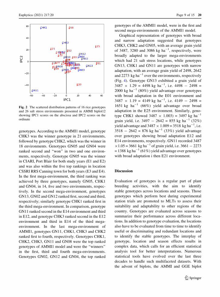
genotypes. According to the AMMI1 model, genotype
CHK3 was the winner genotype in 21 environments,
followed by genotype CHK2, which was the winner in
18 environments. Genotypes GN05 and GN04 were
ranked second and ‘‘won’’ in two and one environ-
ments, respectively. Genotype GN05 was the winner
in CIARI, Port Blair for both study years (E1 and E2)
and was also within the five top rankings in location
CSSRI RRS Canning town for both years (E3 and E4).
In the first mega-environment, the third ranking was
achieved by three genotypes, namely GN05, CHK1
and GN04, in 14, five and two environments, respec-
tively. In the second mega-environment, genotypes
GN13, GN02 and GN12 ranked first, second and third,
respectively; similarly genotype CHK1 ranked first in
the third mega-environment. In comparison, genotype
GN11 ranked second in the E14 environment and third
in E12, and genotype CHK3 ranked second in the E12
environment and third in E14 of the third mega-
environment. In the last mega-environment of
AMMI1, genotypes GN11, CHK1, CHK3 and CHK2
ranked first to fourth, respectively. Genotypes CHK1,
CHK2, CHK3, GN11 and GN08 were the top ranked
genotypes of AMMI1 model and were the ‘‘winners’’
in the first, third and fourth mega-environments.
Genotypes GN02, GN12 and GN04, the top ranked
genotypes of the AMMI1 model, were in the first and
second mega-environments of the AMMI1 model.
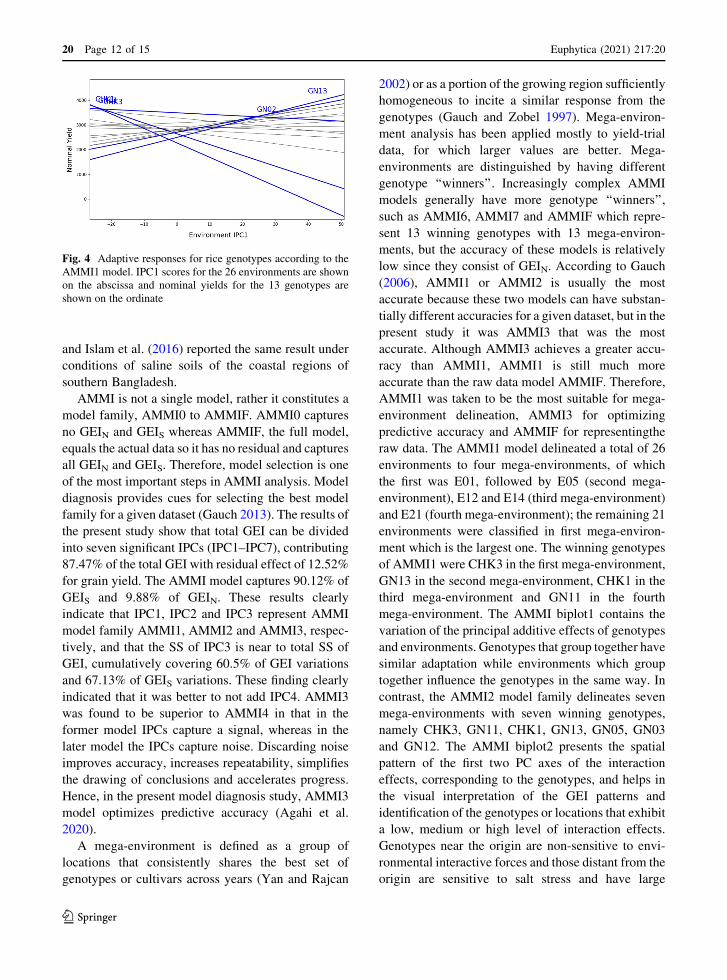
Graphical representation of genotypes with broad
and narrow adaptation suggested that genotypes
CHK3, CHK2 and GN05, with an average grain yield
of 3487, 3280 and 3086 kg ha-1, respectively, were
broadly adapted to the larger mega-environments
which had 21 salt stress locations, while genotypes
GN13, CHK1 and GN11 are genotypes with narrow
adaptation, with an average grain yield of 2498, 2642
and 2273 kg ha-1 over the environments, respectively
(Fig. 4). Genotype GN13 exhibited a grain yield of
3487 9 1.29 = 4498 kg ha-1, i.e. 4498 - 2498 =
2000 kg ha-1 (80%) yield advantage over genotypes
with broad adaptation in the E01 environment and
3487 9 1.19 = 4149 kg ha-1, i.e. 4149 - 2498 =
1651 kg ha-1 (66%) yield advantage over broad
adaptation in the E25 environment. Similarly, geno-
type CHK1 showed 3487 9 1.003) = 3497 kg ha-1
grain yield, i.e. 3497 - 2642 = 855 kg ha-1 (32%)
yield advantage and 3487 9 1.009 = 3518 kg ha-1, i.e.
3518 - 2642 = 876 kg ha-1 (33%) yield advantage
over genotypes showing broad adaptation E12 and
E14 environments, respectively. GN11 recorded 3487
91.05 = 3661 kg ha-1 of grain yield, i.e. 3661 - 2273
= 1388 kg ha-1 (61%) yield advantage over genotypes
with broad adaptation i then E21 environment.
Discussion
Evaluation of genotypes is a regular part of plant
breeding activities, with the aim to identify
stable genotypes across locations and seasons. Those
genotypes which perform best during experimental
station trials are promoted to MLTs to assess their
suitability and adaptability to other regions of the
country. Genotypes are evaluated across seasons to
summarize their performance across different loca-
tions. In addition to genotype evaluation, the locations
also have to be evaluated from time to time to identify
useful or discriminating and redundant locations and
to identify the stable genotypes. The interplay of
genotype, location and season effects results in
complex data, which calls for an efficient statistical
analysis tool for better interpretations. Numerous
statistical tools have evolved over the last three
decades to handle such multifaceted datasets. With
the advent of biplots, the AMMI and GGE biplot
Fig. 2 The scattered distribution patterns of 16 rice genotypes
and 26 salt stress environments presented in AMMI biplot12
showing IPC1 scores on the abscissa and IPC2 scores on the
ordinate
123
Euphytica (2021) 217:20 Page 9 of 15 20
Table
5A
ran
kin
gta
ble
sho
win
gth
eto
pfi
ve
gen
oty
pes
acco
rdin
gto
AM
MI1
and
AM
MIF
mo
del
fam
ilie
sfo
r1
6ri
ceg
eno
typ
es
Meg
a-
env
iro
nm
ent
En
vir
on
men
t
cod
e
IPC
1
sco
re
Rat
ioA
MM
I1ra
nk
sA
MM
IFra
nk
s
12
34
51
23
45
ME
-2E
01
50
.88
1.2
93
GN
13
GN
02
GN
12
GN
04
GN
03
GN
05
GN
04
GN
03
GN
12
GN
13
E2
54
9.6
91
.19
4G
N1
3G
N0
2G
N1
2G
N0
4G
N0
3G
N1
3G
N1
2G
N0
2G
N0
4G
N0
6
ME
-1E
20
18
.32
1.0
0C
HK
3G
N0
4G
N0
5G
N0
2G
N1
2G
N0
2G
N0
5G
N0
8G
N0
4G
N0
3
E0
51
5.1
61
.00
CH
K3
GN
05
GN
04
GN
02
CH
K2
GN
07
GN
12
GN
05
GN
03
GN
09
E0
71
5.1
51
.00
CH
K3
GN
05
GN
04
GN
02
CH
K2
GN
06
GN
01
CH
K2
GN
13
GN
05
E0
31
0.2
01
.00
CH
K3
CH
K2
GN
05
GN
04
GN
12
GN
01
GN
10
GN
05
GN
08
GN
02
E0
84
.85
1.0
0C
HK
3C
HK
2G
N0
5G
N0
4G
N1
0C
HK
1C
HK
3C
HK
2G
N0
4G
N0
3
E1
74
.64
1.0
0C
HK
3C
HK
2G
N0
5G
N0
4G
N1
0G
N0
5G
N0
4G
N1
3C
HK
2G
N0
1
E0
61
.84
1.0
0C
HK
3C
HK
2G
N0
5G
N1
0G
N0
1G
N1
3G
N1
2G
N0
7G
N0
1C
HK
3
E0
21
.79
1.0
0C
HK
3C
HK
2G
N0
5G
N1
0G
N0
1G
N0
5G
N0
6C
HK
1C
HK
3G
N1
2
E1
60
.31
1.0
0C
HK
3C
HK
2G
N0
5G
N1
0G
N0
1G
N0
8G
N1
3G
N0
1G
N1
0G
N1
1
E1
5-
0.5
91
.00
CH
K3
CH
K2
GN
05
GN
10
GN
01
GN
04
GN
09
CH
K3
GN
03
GN
13
E0
4-
0.6
71
.00
CH
K3
CH
K2
GN
05
GN
10
GN
01
CH
K3
GN
12
GN
05
GN
13
CH
K1
E1
8-
0.9
71
.00
CH
K3
CH
K2
GN
05
GN
10
GN
01
CH
K3
GN
04
GN
12
CH
K2
GN
03
E1
9-
2.0
81
.00
CH
K3
CH
K2
GN
05
GN
10
GN
01
GN
03
GN
04
CH
K2
GN
08
GN
11
E1
1-
2.2
01
.00
CH
K3
CH
K2
GN
05
GN
10
GN
01
CH
K3
CH
K2
GN
09
GN
08
GN
07
E1
3-
5.3
11
.00
CH
K3
CH
K2
GN
05
GN
10
CH
K1
CH
K1
CH
K3
GN
06
CH
K2
GN
09
E2
4-
7.9
01
.00
CH
K3
CH
K2
GN
05
CH
K1
GN
10
GN
08
CH
K3
GN
10
CH
K2
GN
07
E2
6-
10
.09
1.0
0C
HK
3C
HK
2C
HK
1G
N0
5G
N1
0C
HK
2C
HK
3G
N0
7G
N1
0C
HK
1
E2
2-
13
.80
1.0
0C
HK
3C
HK
2C
HK
1G
N1
1G
N0
5G
N0
5G
N1
0C
HK
1G
N0
1C
HK
3
E2
3-
17
.24
1.0
0C
HK
3C
HK
2C
HK
1G
N1
1G
N0
8G
N0
8C
HK
3C
HK
2G
N1
0C
HK
1
E1
0-
18
.22
1.0
0C
HK
3C
HK
2C
HK
1G
N1
1G
N0
8G
N0
3G
N1
1C
HK
2C
HK
1C
HK
3
E0
9-
20
.25
1.0
0C
HK
3C
HK
2C
HK
1G
N1
1G
N0
8G
N0
8G
N0
9G
N0
7C
HK
2G
N0
5
ME
-3E
12
-2
3.1
01
.00
3C
HK
1C
HK
3G
N1
1C
HK
2G
N0
8G
N0
7G
N1
0G
N1
1C
HK
1G
N0
8
E1
4-
23
.82
1.0
09
CH
K1
GN
11
CH
K3
CH
K2
GN
08
GN
10
GN
11
GN
01
GN
09
CH
K2
ME
-4E
21
-2
6.6
01
.05
3G
N1
1C
HK
1C
HK
3C
HK
2G
N0
8C
HK
3C
HK
2C
HK
1G
N0
8G
N0
1
123
20 Page 10 of 15 Euphytica (2021) 217:20
method have become more popular. The pros and cons
of these two models have been the subject of much
discussion in recent years, particularly in terms of
which model has the best reliability (Gauch 2006; Yan
et al. 2007; Gauch et al. 2008; Yang et al. 2009; Yan
and Holland 2010). The AMMI model separates G, E,
and GE before applying SVD to GE for a least-square
analysis. The GGE biplot method separates E before
SVD and then attempts to separate G and GE after
applying SVD to both. All SVD-based analyses,
including the AMMI model and GGE method, are
essentially equivalent. The AMMI model completely
separates G, E, and GE, as is required for most
agricultural research purposes and also separates
signal from noise by practicing model diagnosis for
the purpose of gaining accuracy (Gauch 2006; Gauch
et al. 2008). The AMMI model is one of the most
stability models employed to identify general and
specifically adapted rice genotypes under the salinity
and alkaline stress conditions of India (Krishnamurthy
et al. 2015, 2016a, d) and coastal regions of southern
Bangladesh (Islam et al. 2016). Krishnamurthy et al.
(2016a) employed the AMMI and GGE models to
identify a superior genotype for a particular trait using
a genotype-by-trait biplot, and to compare the suit-
ability of the AMMI and GGE biplot for identifying
stable genotypes from 44 cultivars tested across seven
salt stress locations. Hence, in the present study, we
used AMMI analysis to analyze a dataset derived from
13 putative salt-tolerant genotypes along with three
checks tested across 13 different salt stress locations of
India in two growing seasons (2014 and 2015).
ANOVA and model diagnosis ANOVA of the
model provide an opportunity to determine whether
selected AMMI analysis is appropriate for a set of
experiments or not. The sum of squares (SS) for grain
yield, G, E and GEI, all direct outputs from ANOVA,
indicated that the main effects and interaction com-
ponents were significant at p B 0.001). The environ-
ment and interaction component explains the larger
proportion of variation, and the genotypic component
(G) explains the least variation. The total variation of
GEI consists of GEIN and GEIS, with GEIN estimated
simply by multiplying the error mean square (pure
error in the study) by the number of degrees of
freedom (df) of GEI, and GEIS obtained by subtracting
GEIN from GEI (Gauch 2013). The SS for GEIS and
GEIN was found to be 8.96- and 0.98-fold that of the
genotypic (G) main effect, respectively. The results
show that the AMMI model, as used in this study, was
appropriate and worthwhile, since the SS for GEIS is
larger than G and datasets having substantial G and
GEIS and also SS for GEI are not buried in GEIN. The
significant contributions of G, E and GEI for grain
yield under conditions of saline and alkaline soils in
India were reported by Krishnamurthy et al. (2015),
Fig. 3 AMMI1 mega-environment display for 16 rice genotypes evaluated under 26 environments of saline and alkaline conditions.
Environmental means are shown on the abscissa and IPC1 scores are shown on the ordinate
123
Euphytica (2021) 217:20 Page 11 of 15 20
and Islam et al. (2016) reported the same result under
conditions of saline soils of the coastal regions of
southern Bangladesh.
AMMI is not a single model, rather it constitutes a
model family, AMMI0 to AMMIF. AMMI0 captures
no GEIN and GEIS whereas AMMIF, the full model,
equals the actual data so it has no residual and captures
all GEIN and GEIS. Therefore, model selection is one
of the most important steps in AMMI analysis. Model
diagnosis provides cues for selecting the best model
family for a given dataset (Gauch 2013). The results of
the present study show that total GEI can be divided
into seven significant IPCs (IPC1–IPC7), contributing
87.47% of the total GEI with residual effect of 12.52%
for grain yield. The AMMI model captures 90.12% of
GEIS and 9.88% of GEIN. These results clearly
indicate that IPC1, IPC2 and IPC3 represent AMMI
model family AMMI1, AMMI2 and AMMI3, respec-
tively, and that the SS of IPC3 is near to total SS of
GEI, cumulatively covering 60.5% of GEI variations
and 67.13% of GEIS variations. These finding clearly
indicated that it was better to not add IPC4. AMMI3
was found to be superior to AMMI4 in that in the
former model IPCs capture a signal, whereas in the
later model the IPCs capture noise. Discarding noise
improves accuracy, increases repeatability, simplifies
the drawing of conclusions and accelerates progress.
Hence, in the present model diagnosis study, AMMI3
model optimizes predictive accuracy (Agahi et al.
2020).
A mega-environment is defined as a group of
locations that consistently shares the best set of
genotypes or cultivars across years (Yan and Rajcan
2002) or as a portion of the growing region sufficiently
homogeneous to incite a similar response from the
genotypes (Gauch and Zobel 1997). Mega-environ-
ment analysis has been applied mostly to yield-trial
data, for which larger values are better. Mega-
environments are distinguished by having different
genotype ‘‘winners’’. Increasingly complex AMMI
models generally have more genotype ‘‘winners’’,
such as AMMI6, AMMI7 and AMMIF which repre-
sent 13 winning genotypes with 13 mega-environ-
ments, but the accuracy of these models is relatively
low since they consist of GEIN. According to Gauch
(2006), AMMI1 or AMMI2 is usually the most
accurate because these two models can have substan-
tially different accuracies for a given dataset, but in the
present study it was AMMI3 that was the most
accurate. Although AMMI3 achieves a greater accu-
racy than AMMI1, AMMI1 is still much more
accurate than the raw data model AMMIF. Therefore,
AMMI1 was taken to be the most suitable for mega-
environment delineation, AMMI3 for optimizing
predictive accuracy and AMMIF for representingthe
raw data. The AMMI1 model delineated a total of 26
environments to four mega-environments, of which
the first was E01, followed by E05 (second mega-
environment), E12 and E14 (third mega-environment)
and E21 (fourth mega-environment); the remaining 21
environments were classified in first mega-environ-
ment which is the largest one. The winning genotypes
of AMMI1 were CHK3 in the first mega-environment,
GN13 in the second mega-environment, CHK1 in the
third mega-environment and GN11 in the fourth
mega-environment. The AMMI biplot1 contains the
variation of the principal additive effects of genotypes
and environments. Genotypes that group together have
similar adaptation while environments which group
together influence the genotypes in the same way. In
contrast, the AMMI2 model family delineates seven
mega-environments with seven winning genotypes,
namely CHK3, GN11, CHK1, GN13, GN05, GN03
and GN12. The AMMI biplot2 presents the spatial
pattern of the first two PC axes of the interaction
effects, corresponding to the genotypes, and helps in
the visual interpretation of the GEI patterns and
identification of the genotypes or locations that exhibit
a low, medium or high level of interaction effects.
Genotypes near the origin are non-sensitive to envi-
ronmental interactive forces and those distant from the
origin are sensitive to salt stress and have large
Fig. 4 Adaptive responses for rice genotypes according to the
AMMI1 model. IPC1 scores for the 26 environments are shown
on the abscissa and nominal yields for the 13 genotypes are
shown on the ordinate
123
20 Page 12 of 15 Euphytica (2021) 217:20
interactions. The points of either genotypes or envi-
ronments that are close to each other have similar
interaction patterns, while those that are distant from
each other have different interaction patterns (Krish-
namurthy et al. 2016d). The AMMI3 model family,
diagnosed as being the most accurate for the present
dataset, delineates ten mega-environments with ten
winning genotypes, namely CHK3, CHK2, GN11,
CHK1, GN06, GN13, GN02, GN03, GN05 and GN08
(Table 4). Among the winning genotypes of the
AMMI 3 model family, genotypes CHK2 and GN05
achieved the second or third ranking in the majority of
the environments of the first mega-environment,
whereas GN02 ranked second in the second mega-
environment of the AMMI1 model family. Finally,
after combining all of the data of this model family, the
overall winning genotypes were CHK3, CHK2, GN11,
CHK1, GN13, GN02 and GN05, which were ranked
either first or second in the mega-environment of the
AMMI1 model family. The ‘‘winner’’ in 1 of the
2 years was not even among the top five genotypes in
the other year in many locations. Since soil salinity is
highly dynamic in nature, the level of salinity changes
with fluctuating environmental factors, such as pre-
cipitation, temperature and relative humidity (Tack
et al. 2015). In our experiment, this is evident by the
effect of environment and GEI being very high
compared to the genotypic effect. The rank of the
genotypes and the performance of the genotypes under
salt stress could be seen to be definitely altered with
varying levels of salt stress (pH and EC of each
location is givenin Table 1). Location (CSSRI, Karnal
sodic microplot, Haryana; namely environments 23
and 24) has four of five common genotypes between
2014 and 2015.
Selection or recommendation of the best genotypes
involves two principal considerations. First, selection
must done in the context mega-environment scheme,
which includes a single mega-environment exploiting
only broad adaptation, or multiple mega-environments
exploiting both broad and narrow adaptation. Second,
selection is based on yield estimates using both the
treatment and experimental designs (Gauch 2013).
According to Gauch (2013), a ratio of 1 represents a
winning genotype across environments. This ratio
assesses the importance of narrow adaptation due to
GEI effects, and a ratio of C 1.10 is indicative of
narrow adaptation. The ratio is the yield (or whatever
the trait) of the winner within each environment,
divided by the yield for the overall winner (which is
CHK3), with both yields estimated by the AMMI1
model, with the ratio automatically equal to 1 for the
overall winner. This ratio assesses the importance of
narrow adaptation, which are caused by G 9 E
interactions. When a 5 or 10% yield increment has
agricultural or economic significance, a ratio of C 1.10
indicates that narrow adaptation offers substantial
opportunities for yield increases, although at the cost
of subdividing a growing region into two or more
mega-environments. Therefore, CHK3, CHK2 and
GN05 were the winning genotypes, with a ratio of 1;
they are broadly adopted for different stress environ-
ments. In contrast, genotypes GN13 and GN02
showed narrow adaptation to E01, with a 29% yield
advantage, and to E05, with a 19% yield advantage
over the winning genotype (CHK3) under broad
adaptation. Similarly. CHK1 adapted to E12 and E14
with negligible yield increment and GN11 adapted
specifically to E21 with a 5% yield increment over the
winning genotype (CHK3) under broad adaptation.
The checks continued to dominate the genotypes in
terms of high yields and stability, and this issue has to
be seriously looked into by breeders. Stable rice
genotypes have been identified across salt stress
locations previously by Kumar et al.
(2007, 2010, 2011), Anandan et al. (2009), Ali et al.
(2013), Krishnamurthy et al. (2014) and Krishna-
murthy et al. (2016b, 2017).
The genotypes GN13 and GN02 were narrowly
adapted, with positive GEI in second mega-environ-
ment and negative GEI in the third and fourth mega-
environments and also in the majority of the environ-
ments of the first mega-environment. Genotypes
CHK3, CHK2 and GN05 were showed broad adapta-
tion with neutral GEI and were less sensitive to the
dynamic conditions of the salt stress condition. CHK1
and GN11 were narrow-adapted genotypes with
positive GEI in the third and fourth mega-environment
and in some of the environments of the first mega-
environments, and with negative GEI in the second
mega-environment. In the present investigation, the
three broadly adapted, stable winning genotypes,
namely CHK3, CHK2 and GN05, were identified,
with a maximum grain yield of 3487.82, 3280 and
3086.29 kg ha-1, respectively, which is more than
grand mean yield of 2828.28 kg ha-1. Genotypes
GN13, CHK1 and GN11 were narrowly adapted to the
second, third and fourth mega-environments,
123
Euphytica (2021) 217:20 Page 13 of 15 20

respectively. Genotype GN13 recorded 80% yield
advantage in the E01 environment and 66% yield
advantage in E25. Similarly, GN11 provided 61%
yield advantage in the E21 environment. Based on
these findings, these three genotypes could be recom-
mended for specific mega-environments.
Conclusion
The aim of the present study was to evaluate
geographically and genetically diverse putative salt-
tolerant rice genotypes across 13 salt stress locations
representing inland salinity, alkalinity and coastal
salinity conditions across India using the AMMI
stability model. We found that the study locations
themselves were significant factors accounting for the
total variation in grain yield. This finding makes plant
breeding efforts even more challenging, and a great
deal of effect is needed to pool data from more number
of years and to correlate it with weather changes and
salinity dynamics during the period being studied. In
our study, variety CSR 36 (CHK3) was found to be the
most ideal and stable candidate, followed by IR
87952-1-1-1-2-3-B (G05). Overall, the most promis-
ing genotypes (CSR 36 [CHK3], IR 87952-1-1-1-2-3-
B [GN05] and CST27 [CHK2]) had high mean yield
and stability, and IR 87952-1-1-1-2-3-B (GN05) could
be used for commercial cultivation across salt-affected
soils. GN13 (IR 87938-1-1-2-1-3-B) and GN11 (IR
87938-1-2-2-1-3-B) were winning genotypes and are
recommended for second and fourth mega-environ-
ments, with 61–80% yield advantages in narrow
adaptation over broad adaptation.
Acknowledgements The authors sincerely thank the Bill and
Melinda Gates Foundation for funding support under the
STRASA project (IRRI-ICAR collaborative project), and the
Directors of all the partner institutes for encouragement. The
authors also thank to the Director, ICAR CSSRI, for support.
PME cell reference- RA/91/2019.
Open Access This article is licensed under a Creative Com-
mons Attribution 4.0 International License, which permits use,
sharing, adaptation, distribution and reproduction in any med-
ium or format, as long as you give appropriate credit to the
original author(s) and the source, provide a link to the Creative
Commons licence, and indicate if changes were made. The
images or other third party material in this article are included in
the article’s Creative Commons licence, unless indicated
otherwise in a credit line to the material. If material is not
included in the article’s Creative Commons licence and your
intended use is not permitted by statutory regulation or exceeds
the permitted use, you will need to obtain permission directly
from the copyright holder. To view a copy of this licence, visit
http://creativecommons.org/licenses/by/4.0/.
Author’s contribution SLK, PCS, DKS, AMI and RKS
conceptualized and designed the experiment. SLK, YPS,
VKM, DB, BM, SM, SKS, RKG, PKS, KKM, BCM, KC, GP,
PBV KDP, ST, OPV, AHK, ST, SG, RG, VKY, SKBR, MP and
AA performed the field evaluations and recorded data. SLK and
JB performed the data analysis. SLK drafted and revised the
manuscript. PCS, DKS, AMI, RKS, YPS, VKM, DB, BM, SM,
SKS, RKG, PKS, KKM, BCM, KC, GP, PBV KDP, ST, OPV,
AHK, ST, SG, RG, VKY, SKBR, MP and AA edited the
manuscript. All authors have read and approved the final
manuscript.
References
Agahi K, Ahmadi J, Oghan HA, Fotokian MH, Orang SF (2020)
Analysis of genotype 9 environment interaction for seed
yield in spring oilseed rape using the AMMI model. Crop
Br Appl Biotechnol 20(1):e26502012. https://doi.org/10.
1590/1984
Ali S, Gautam RK, Mahajan R, Krishnamurthy SL, Sharma SK,
Singh RK, Ismail AM (2013) Stress indices and
selectable traits in SALTOL QTL introgressed rice geno-
types for reproductive stage tolerance to sodicity and
salinity stresses. Field Crops Res 154:65–73
Anandan A, Eswaran R, Sabesan T, Prakash M (2009) Additive
main effects and multiplicative interactions analysis of
yield performances in rice genotypes under coastal saline
environments. Adv Biol Res 3(1–2):43–47
Cornelius PL (1993) Statistical tests and retention of terms in the
additive main effects and multiplicative interaction model
for cultivar trials. Crop Sci 33:1186–1193
Ebdon JS, Gauch HG (2002a) Additive main effect and multi-
plicative interaction analysis of national turfgrass perfor-
mance trials: I. Interpretation of genotype 9 environment
interaction. Crop Sci 42:489–496
Ebdon JS, Gauch HG (2002b) Additive main effect and multi-
plicative interaction analysis of national turfgrass perfor-
mance trials: II. Cultivar recommendation. Crop Sci
42:497–506
FAO (Food and Agricultural Organization of the United
Nations) (2014) Extent of salt affected soils. www.fao.org/
soils-portal/soil-management/management-of-
someproblem-soils/salt-affected-soils/more-information-
on-saltaffected-soils/en/. Accessed 3 December 2014
Gabriel KR (1971) The biplot graphic display of matrices with
application to principal component analysis. Biometrika
58:453–467
Gauch HG (1992) AMMI analysis of yield trials. In: Kang MS,
Gauch HG (eds) Genotype-by-environment interaction.
CRC Press, Boca Raton, pp 1–40
123
20 Page 14 of 15 Euphytica (2021) 217:20
Gauch HG (2006) Statistical analysis of yield trials by AMMI
and GGE. Crop Sci 46:1488–1500
Gauch HG (2013) A simple protocol for AMMI analysis of yield
trials. Crop Sci 53:1860–1869
Gauch HG, Zobel RW (1997) Identifying mega-environments
and targeting genotypes. Crop Sci 37:311–326
Gauch HG, Piepho HP, Annicchiarico P (2008) Statistical
analysis of yield trials by AMMI and GGE: further con-
siderations. Crop Sci 48:866–889
Islam MR, Sarkerb MRA, Sharmab N, Rahmanb MA, Collarda
BCY, Gregorio GB, Ismail AM (2016) Assessment of
adaptability of recently released salt tolerant rice varieties
in coastal regions of South Bangladesh. Field Crops Res
190:34–43
Krishnamurthy SL, Sharma SK, Gautam RK, Kumar V (2014)
Path and association analysis and stress indices for salinity
tolerance traits in promising rice (Oryza sativa L.) geno-
types. Cereal Res Commun 42(3):474–483. https://doi.org/
10.1556/crc.2013.0067
Krishnamurthy SL, Pundir P, Singh YP, Sharma SK, Sharma
PC, Sharma DK (2015) Yield stability of rice lines for salt
tolerance using additive main effects and multiplicative
interaction analysis—AMMI. J Soil Salin Water Qual
7(2):98–106
Krishnamurthy SL, Sharma PC, Ravikiran KT, Nirmalendu
Basak TV, Vineeth YPSingh, Sarangi SK (2016a) G 9 E
interaction and stability analysis for salinity and sodicity
tolerance in rice at reproductive stage. J Soil Salin Water
Qual 8(2):54–64
Krishnamurthy SL, Sharma PC, Sharma SK, Batra V, Kumar V
(2016b) Effect of salinity and use of stress indices of
morphological and physiological traits at the seedling stage
in rice. Indian J Exp Biol 54(12):843–850
Krishnamurthy SL, Gautam RK, Sharma PC, Sharma DK
(2016c) Effect of different salt stresses on agro-morpho-
logical traits and utilization of salt stress indices for
reproductive stage salt tolerance in rice. Field Crops Res
190:26–33. https://doi.org/10.1016/j.fcr.2016.02.018
Krishnamurthy SL, Sharma SK, Sharma DK, Sharma PC, Singh
YP, Mishra VK, Burman D, Maji B, Bandyopadhyay BK,
Mandal S, Sarangi SK, Gautam RK, Singh PK, Manohara
KK, Marandi BC, Singh DP, Padmavathi G, Vanve PB,
Patil KD, Thirumeni S, Verma OP, Khan AH, Tiwari S,
Shakila M, Ismail AM, Gregorio GB, Singh RK (2016d)
Analysis of stability and G 9 E interaction of rice geno-
types across saline and alkaline environments in India.
Cereal Res Commun 44(2):349–360. https://doi.org/10.
1556/0806.43.2015.055
Krishnamurthy SL, Sharma PC, Sharma DK, Ravikiran KT,
Singh YP, Mishra VK, Burman D, Buddheswar Maji S,
Mandal SKSarangi, Gautam RK, Singh PK, Manohara KK,
Marandi BC, Padmavathi G, Vanve PB, Patil KD, Thiru-
meni S, Verma OP, Khan AH, Tiwari S, Geetha S, Shakila
M, Gill R, Yadav VK, Roy B, Prakash M, Bonifacio J,
Ismail AbdelbagiM, Gregorio GB, Singh RK (2017)
Identification of mega-environments and rice genotypes for
general and specific adaptation to saline and alkaline
stresses in India. Sci Rep 7:7968. https://doi.org/10.1038/
s41598-017-08532-7
Kumar DBM, Thyagaraj NE, Ramachandra C, Krishnamurthy
SL (2007) Stability analysis for grain yield and yield
components in red rice. Int J Agric Sci 3(1):145–147
Kumar DBM, Shadakshari YG, Krishnamurthy SL (2010)
Genotype 9 environment interaction and stability analysis
for grain yield and its components in Halugidda local rice
mutants. Electron J Plant Breed 1(5):1286–1289
Kumar DBM, Gangaprsad S, Krishnamurthy SL, Mallikarju-
naiah H (2011) Stability analysis of puttabatta rice mutants.
Karnataka J Agric Sci 24(4):527–528
Mohammadi R, Mendioro MS, Diaz GQ, Gregorio GB, Singh
RK (2013) Mapping quantitative trait loci associated with
yield and yield components under reproductive stage
salinity stress in rice (Oryza sativa L.). J Genet 92:433–443
Mondal AK, Sharma RC, Singh GB (2009) Assessment of salt
affected soils in India using GIS. Geocarto Int
24(6):437–456
Munns R, Tester M (2008) Mechanisms of salinity tolerance.
Annu Rev Plant Biol 59:651–681
Singh RK, Flowers TJ (2010) The physiology and molecular
biology of the effects of salinity on rice. In: Pessarakli M
(ed) Handbook of plant and crop stress, 3rd edn. Taylor and
Francis, Boca Raton, pp 901–942
Tack J, Singh RK, Nalley LL, Viraktamath BC, Krishnamurthy
SL, Lyman N, Jagadish KSV (2015) High vapor pressure
deficit drives salt-stress induced rice yield losses in India.
Glob Chang Biol 21:1668–1678
Wu R, Garg A (2003) Engineering rice plants with trehalose-
producing genes improves tolerance to drought, salt and
low temperature. ISBN News Report, February 2003.
http://www.isb.vt.edu/
Yan W, Holland JB (2010) A heritability-adjusted GGE biplot
for test environment evaluation. Euphytica 171:355–369
Yan W, Rajcan I (2002) Biplot evaluation of test sites and trait
relations of soybean in Ontario. Crop Sci 42:11–20
Yan W, Hunt LA, Sheng Q, Szlavnics Z (2000) Cultivar eval-
uation and mega-environment investigation based on GGE
biplot. Crop Sci 40:597–605
Yan W, Kang MS, Ma BL, Woods S, Cornelius PL (2007) GGE
biplot vs. AMMI analysis of genotype-by-environment
data. Crop Sci 47:643–655
Yang RC, Crossa J, Cornelius PL, Burgueno J (2009) Biplot
analysis of genotype 9 evironment interaction: proceed
with caution. Crop Sci 49:1564–1576
Zobel RW, Wright MJ, Gauch HG (1988) Statistical analysis of
a yield trial. Agron J 80:388–393
Publisher’s Note Springer Nature remains neutral with
regard to jurisdictional claims in published maps and
institutional affiliations.
123
Euphytica (2021) 217:20 Page 15 of 15 20