adaptivecontrolandsynchronization ofamodiﬁedchua...

Adaptive control and synchronizationof a modified Chua’s circuit system

M.T. Yassen

Mathematics Department, Faculty of Science, Mansoura University, Mansoura 35516, Egypt

Abstract

This study addresses the adaptive control and synchronization of the modified

Chua’s circuit system with unknown system parameters. Adaptive control law is applied

to suppress chaos to one of the three steady states. Adaptive control law is applied to

achieve synchronization of two identical modified Chua’s circuit systems. Routh–

Hurwitz criteria and Lyapunov direct method are used to study the asymptotic stability

of the steady states. Numerical simulations are included to show the effectiveness of the

proposed control method.

� 2002 Elsevier Science Inc. All rights reserved.

1. Introduction

Research efforts have investigated the chaos control and chaos synchroni-

zation problems in many physical chaotic systems [1–13]. The control problem

attempts to stabilize a chaotic attractor to either a periodic orbit or an equi-

librium point. Recently, after the pioneering work of Ott et al. [1], several

control strategies for stabilizing chaos have been proposed. There are two mainapproaches for controlling chaos, nonfeedback control [2,3] and feedback

control [4,13].

The concept of chaos synchronization involves making two chaotic systems

which oscillate in a synchronized manner. The idea of synchronizing two

identical chaotic systems with different initial conditions was introduced by

Pecora and Carrol [14].

E-mail address: [email protected] (M.T. Yassen).

0096-3003/02/$ - see front matter � 2002 Elsevier Science Inc. All rights reserved.

PII: S0096 -3003 (01 )00318-6

Applied Mathematics and Computation 135 (2003) 113–128

www.elsevier.com/locate/amc

mail to: [email protected]

Several different approaches, including some conventional linear control

techniques and advanced nonlinear control schemes, are already applied to theabove problems. In these works, it is essential to know the values of system

parameters. In practical situations, the values of these parameters are un-

known. Therefore, the derivation of an adaptive controller for the control and

synchronization of chaotic systems in the presence of unknown parameters is

an important issue [15–18].

Chua’s circuit has been studied extensively as a prototypical electronic

system [19]. Chen and Dong [5,6] applied the linear feedback control for

guiding the chaotic trajectory of the circuit to limit cycle. Hartley and Moss-ayebi [8] showed the control of modified Chua’s circuit systems and demon-

strated how to design a controller for tracking the capacitor voltage of the

system by applying the input–output and state space techniques. Saito and

Mitsubori [9] stabilized chaotic attractor to desired periodic orbit by proposing

a simple control method. Hwang et al. [10] proposed a feedback control on a

modified Chua’s circuit to drag the chaotic trajectory to fixed points. The

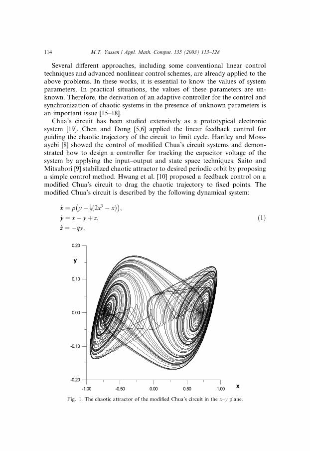
modified Chua’s circuit is described by the following dynamical system:

_xx ¼ p y�

� 17ð2x3 � xÞ

�;

_yy ¼ x� y þ z;

_zz ¼ �qy;

ð1Þ

Fig. 1. The chaotic attractor of the modified Chua’s circuit in the x–y plane.

114 M.T. Yassen / Appl. Math. Comput. 135 (2003) 113–128

where p > 0 and q > 0 are system parameters, x and y are the voltages across

two capacitors and z is the current through the inductor. The system (1) hasthree equilibrium points Eþ ¼ ð

ffiffiffiffi:5

p; 0;�

ffiffiffiffi:5

pÞ, E0 ¼ ð0; 0; 0Þ and E� ¼ ð�

ffiffiffiffi:5

p; 0;ffiffiffiffi

:5p

Þ. The chaotic attractor of the system (1) in the x–y plane is shown in Fig. 1.

The aim of this paper is to introduce a simple, smooth and adaptive con-

troller for resolving the control and synchronization problems of the modified

Chua’s circuit systems. It is assumed that the two parameters p and q are

unknown and only a single state variable is available for implementing the

feedback controller. In Section 2, the stability of the equilibrium points Eþ, E0and E� is studied. In Section 3, feedback control and adaptive control arestudied. In Section 4, adaptive synchronization of two identical modified

Chua’s circuits is studied. In Section 5, numerical simulation is presented.

Section 6 is the conclusion.

Remark 1. The system has a bounded, zero volume, globally attracting set [20].

Therefore, the state trajectories xðtÞ, yðtÞ; and zðtÞ are globally bounded for alltP 0 and continuously differentiable with respect to time. Consequently, there

exist three positive constants s1, s2 and s3 such that jxðtÞj6 s1 < 1,jyðtÞj6 s2 < 1 and jzðtÞj6 s3 < 1 hold for all tP 0.

2. Stability of the equilibrium points

Proposition 1. For p ¼ 10 and q ¼ 1007, the three equilibrium points Eþ, E0 and E�

of the system (1) are unstable.

Proof. The Jacobian matrix of the system (1) about the equilibrium point

E ¼ ð�xx; �yy;�zzÞ is

J0 ¼pð�6�xx2þ1Þ

7p 0

1 �1 1

0 �q 0

264

375:

The characteristic equation of J0 is

k3 þ 1

þ pð6�xx2 � 1Þ

7

!k2 þ q

"þ p

6�xx2 � 87

!#k þ pqð6�xx2 � 1Þ

7¼ 0:

Let

b1 ¼ 1þpð6�xx2 � 1Þ

7; b2 ¼ qþ p

6�xx2 � 87

!and b3 ¼

pqð6�xx2 � 1Þ7

:

M.T. Yassen / Appl. Math. Comput. 135 (2003) 113–128 115

For p ¼ 10 and q ¼ 1007: Firstly, if �xx ¼ 0, then b1 < 0 and b3 < 0. According to

Routh–Hurwitz criteria the equilibrium point ð0; 0; 0Þ is unstable. Secondly, if�xx ¼

ffiffiffiffi:5

p, then b1 > 0, b2 > 0 and b1b2 < b3. According to Routh–Hurwitz

criteria the equilibrium points Eþ ¼ ðffiffiffiffi:5

p; 0;�

ffiffiffiffi:5

pÞ and E� ¼ ð�

ffiffiffiffi:5

p; 0;

ffiffiffiffi:5

pÞ

are unstable.

Since the equilibrium points of system (1) are unstable, the control problem

takes place. �

3. Adaptive control

Let us consider the controlled system of the system (1) has the form

_xx ¼ p y�

� 17ð2x3 � xÞ

�þ u1;

_yy ¼ x� y þ zþ u2;

_zz ¼ �qy þ u3;

ð2Þ

where u1, u2 and u3 are external control inputs which will drag the chaotictrajectory ðx; y; zÞ of the modified Chua system (1) to E ¼ ð�xx; �yy;�zzÞ one of thethree steady states E�, E0 and Eþ. Let the control law take the following form:

u1 ¼ �kðx� �xxÞ; u2 ¼ u3 ¼ 0;

where k is a positive feedback gain.

3.1. Stabilizing the equilibrium point E ¼ ðx; y; zÞ

In order to suppress chaos to E ¼ ð�xx; �yy;�zzÞ, we introduce the external controllaw u1 ¼ �kðx� �xxÞ; u2 ¼ u3 ¼ 0 with x as the feedback variable into system (2).Hence the controlled system (2) has the following form:

_xx ¼ p y�

� 17ð2x3 � xÞ

�� kðx� �xxÞ;

_yy ¼ x� y þ z;

_zz ¼ �qy:

ð3Þ

The controlled system (3) has the equilibrium point E ¼ ð�xx; �yy;�zzÞ. The system (3)can be stabilized to the steady state E ¼ ð�xx; �yy;�zzÞ if k P k is satisfied and thesystem parameters are constant and known.

Let us consider that n1 ¼ x� �xx, n2 ¼ y � �yy, n3 ¼ z��zz and a ¼ pð17ð�6�xx2 þ 1ÞÞ:

Proposition 2. The equilibrium point E ¼ ð�xx; �yy;�zzÞ of the system (3) is asymp-totically stable for kP k ¼ p þ a, where p; q are positive.


Proof. The Jacobian matrix of the system (3) about the equilibrium point

E ¼ ð�xx; �yy;�zzÞ is

J ¼pð�6�xx2þ1

7Þ � k p 0

1 �1 1

0 �q 0

24

35: ð4Þ

The linearized system of (3) is given by

_nn1 ¼ ða � kÞn1 þ pn2;_nn2 ¼ n1 � n2 þ n3;

_nn3 ¼ �qn2:

ð5Þ

We study the stability of the equilibrium point ð0; 0; 0Þ of the system (5).

Consider the Lyapunov function V ðn1; n2; n3Þ is

V ðn1; n2; n3Þ;¼1

2

qp

n21

�þ qn22 þ n23

�: ð6Þ

The time derivative of V in the neighbourhood of ð0; 0; 0Þ is

_VV ¼ �qðn2 � n1Þ2 �qn21p

ðk � a � pÞ:

It is clear that _VV < 0 if kP k ¼ p þ a. According to Lyapunov stability theorythe equilibrium point ð0; 0; 0Þ is asymptotically stable. �

Remark 2. The chaotic attractor of the modified Chua circuit ðx; y; zÞ is sup-pressed to a limit cycle around the equilibrium point E0 ¼ ð0; 0; 0Þ by takingk ¼ 9:9152 in (3) (see Fig. 5).

The feedback control law derived thus far requires that the system parame-ters must be known a priori. However, in many real applications it can be

difficult to determine exactly the values of the system parameters. Consequently,

the feedback gain k cannot be appropriately chosen to guarantee the stability ofthe controlled system. For overestimating k an expensive and too conservativecontrol effort is needed. To overcome these drawbacks, an adaptive control with

single state variable feedback control is derived.

An adaptive control with x as the feedback variable is added into the firstequation in system (2). In this case the control law is

u1 ¼ �gðx� �xxÞ; u2 ¼ u3 ¼ 0; ð7Þ

where g, an estimate of g1, is updated according to the following adaptive al-gorithm:


_gg ¼ cðx� �xxÞ2; ð8Þ

where c is an adaption gain. Then the controlled system (2) has the followingform:

_xx ¼ p y�

� 17ð2x3 � xÞ

�� gðx� �xxÞ;

_yy ¼ x� y þ z;

_zz ¼ �qy;

_gg ¼ cðx� �xxÞ2:

ð9Þ

Proposition 3. For g ¼ g1P p þ a and p; q are positive, the equilibrium pointE ¼ ð�xx; �yy;�zzÞ of the system (9) is asymptotically stable.

Proof. Let us consider the Lyapunov function as follows:

V ¼ 12

qpðx

�� xxÞ2 þ qðy � �yyÞ2 þ ðz� �zzÞ2 þ q

cpðg � g1Þ2

�: ð10Þ

The time derivative of V in the neighbourhood of the equilibrium point ð�xx; �yy;�zzÞof the system (9) is

_VV ¼ qðx� �xxÞ y�

� 17ð2x3 � xÞ

�� qg

pðx� �xxÞ2 þ qðy � �yyÞðx� y þ zÞ

�qyðz� �zzÞ þ qpðg � g1Þðx� �xxÞ2:

Put g1 ¼ x� �xx, g2 ¼ y � �yy and g3 ¼ z� �zz. Since ð�xx; �yy;�zzÞ is an equilibrium pointof the uncontrolled system (1), then _VV becomes

_VV ¼ qg1 g2

�� 17ð2g31 � g1Þ �

1

7ð6�xx2g1 þ 6�xxg21Þ

�þ qg2ðg1 � g2 þ g3Þ

� qg2g3 þqpðg � g1Þg21

¼ 2qg1g2 �2q7

g41 � qg21g1p

� 17þ 6�xx

2

7

!� 6q�xxg

31

7� qg22

¼ �qðg2 � g1Þ2 � qg21

g1p

"� 1

þ ð�6�xx2 þ 1Þ

7

!#� 6q�xxg

31

7:

It is clear that for the positive parameters p, q and c, if we choose g ¼ g1 Pp þ a and jg1j is sufficiently small, then _VV is negative definite and from (10) theLyapunov function V is positive definite. From Lyapunov stability theorem it


follows that the equilibrium point x ¼ �xx, y ¼ �yy, z ¼ �zz, g ¼ g1 of the system (9) isasymptotically stable. �

4. Adaptive synchronization

We assume that we have two modified Chua’s circuit systems and that the

drived system with the subscript 1 drives the response system with the subscript

2. The systems are

_xx1 ¼ p y1�

� 17ð2x31 � x1Þ

�;

_yy1 ¼ x1 � y1 þ z1;

_zz1 ¼ �qy1

ð11Þ

and

_xx2 ¼ p y2�

� 17ð2x32 � x2Þ

�þ u;

_yy2 ¼ x2 � y2 þ z2;

_zz2 ¼ �qy2:

ð12Þ

We have introduced the control input u into the first equation in the system(12). This input is to be determined for the purpose of synchronizing the two

identical modified Chua’s circuit systems with the same but unknown para-

meters p and q. Let us define the state errors between the response system (12)and the derive system (11) as follows:

ex ¼ x2 � x1; ey ¼ y2 � y1; ez ¼ z2 � z1: ð13Þ

Subtracting Eq. (11) from Eq. (12) and using the notation (13) yields

_eex ¼ p ey

�� 27ðx32 � x31Þ þ

ex7

�þ u;

_eey ¼ ex � ey þ ez;

_eez ¼ �qey :

ð14Þ

Eq. (14) describes the error dynamics. It is clear that the synchronization

problem is replaced by the equivalent problem of stabilizing the system (14)using a suitable choice of the control law u. The synchronization problem forthe modified Chua circuit is to achieve the asymptotic stability of the zero

solution of the error system (14) in the sense that

keðtÞk ! 0 as t ! 1;

where eðtÞ ¼ ðexðtÞ; eyðtÞ; ezðtÞÞ. For this purpose we consider the control law asfollows:


u ¼ �hex; ð15Þ

where h is an estimated feedback gain which is updated according to the fol-lowing adaption algorithm:

_hh ¼ ce2x ; hð0Þ ¼ 0: ð16Þ

Then the controlled resulting error system (14) can be expressed by the fol-

lowing dynamical system:

_eex ¼ p ey

�� 27ðx32 � x31Þ þ

ex7

�� hex;

_eey ¼ ex � ey þ ez;

_eez ¼ �qey ;_hh ¼ ce2x :

ð17Þ

Proposition 4. The zero solution of the error system (17) is asymptotic stable forh ¼ h1 P pð1þ 2

7aÞ, where a ¼ x22 þ x1x2 þ x21.

Proof. Let us consider Lyapunov function is

V ¼ 12

qpe2x

�þ qe2y þ e2z þ

qcp

ðh� h1Þ2�; ð18Þ

where h1 is a positive constant. The time derivative of Eq. (18) in the neigh-bourhood of the zero solution of the system (17) is

_VV ¼ �qðey � exÞ2 þqpe2xðp � h1Þ �

2q7e2xðx22 þ x1x2 þ x21Þ:

It is clear that x22 þ x1x2 þ x21 is positive for all xi 2 R, i ¼ 1; 2. Let a ¼ x22þx1x2 þ x21. Then _VV can be rewritten in the following form:

_VV ¼ �qðey � exÞ2 �qpe2x h1

�� p � 2p

7a�: ð19Þ

From (19) and for the positive parameters p, q and c it is clear that if we takeh ¼ h1 P pð1þ 2

7aÞ, then _VV is negative definite and from (18) the Lyapunov

function V is positive definite. From Lyapunov stability theorem it follows thatthe equilibrium points ex ¼ 0, ey ¼ 0, ez ¼ 0, h ¼ h1 of the system (17) is h,asymptotic stable. The proof is completed. �


5. Numerical simulation

We will show a series of numerical experiments to demonstrate the effec-

tiveness of the proposed control scheme. Fourth-order Runge–Kutta method is

used to integrate the differential equations with time step 0.01. The parameters

p, q and c are chosen p ¼ 10, q ¼ 1007and c ¼ 1 in all simulations to ensure the

existence of chaos in the absence of control. The initial states are taken

x ¼ :65; y ¼ 0; z ¼ 0 in the controlling chaos problem, however, x1 ¼ :65,y1 ¼ 0 and z1 ¼ 0 of the derive system and x2 ¼ :2, y2 ¼ :1 and z2 ¼ :1 of theresponse system are chosen in the synchronization problem.

5.1. Chaos control to equilibrium points

5.1.1. Feedback control

The equilibrium point E0 ¼ ð0; 0; 0Þ of the system (2) is stabilized for

k1 ¼ 12: Fig. 2 shows that the chaos is suppressed to the equilibrium point E0with time. The control is activated at t ¼ 20. The equilibrium point Eþ ¼ðffiffiffiffi:5

p; 0;�

ffiffiffiffi:5

pÞ of the system (2) is stabilized for k1 ¼ 8: Fig. 3 shows that the

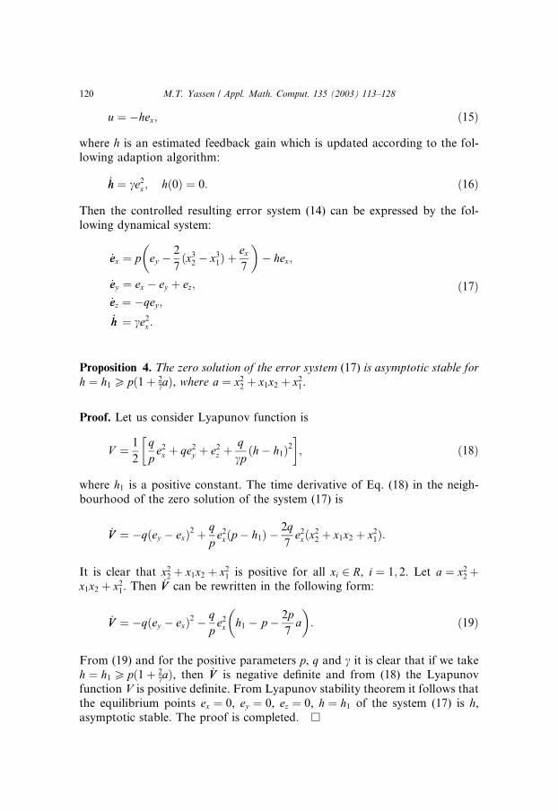
chaotic trajectory can be stabilized to the equilibrium point Eþ with time. The

control is activated at t ¼ 20: Fig. 4 shows the stabilization of the equilib-rium point E� ¼ ð�

ffiffiffiffi:5

p; 0;

ffiffiffiffi:5

pÞ of the system (2) where k1 ¼ 8. The control is

Fig. 2. The stabilization of the equilibrium point E0 of the system (2). The control law u1 ¼ �12x;u2 ¼ u3 ¼ 0 is activated at t ¼ 20.


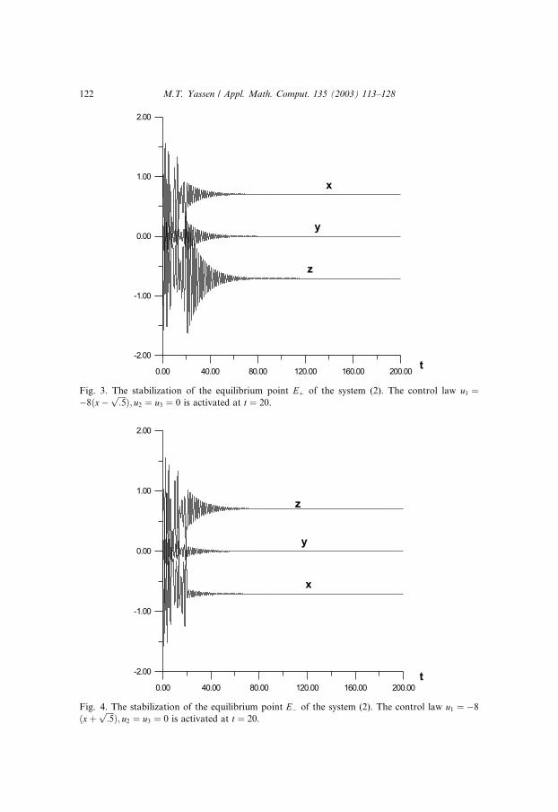
Fig. 3. The stabilization of the equilibrium point Eþ of the system (2). The control law u1 ¼�8ðx�

ffiffiffiffi:5

pÞ; u2 ¼ u3 ¼ 0 is activated at t ¼ 20.

Fig. 4. The stabilization of the equilibrium point E� of the system (2). The control law u1 ¼ �8ðxþ

ffiffiffiffi:5

pÞ; u2 ¼ u3 ¼ 0 is activated at t ¼ 20.


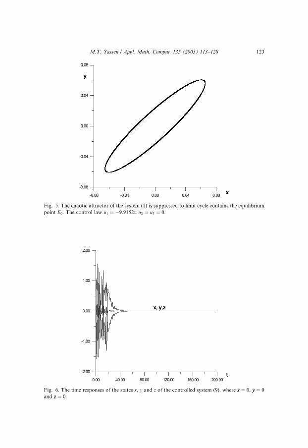
Fig. 5. The chaotic attractor of the system (1) is suppressed to limit cycle contains the equilibrium

point E0. The control law u1 ¼ �9:9152x; u2 ¼ u3 ¼ 0.

Fig. 6. The time responses of the states x, y and z of the controlled system (9), where �xx ¼ 0, �yy ¼ 0and �zz ¼ 0.


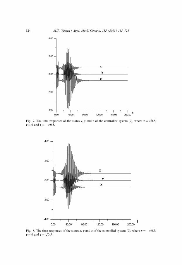
Fig. 7. The time responses of the states x, y and z of the controlled system (9), where �xx ¼ffiffiffiffiffiffiffi0:5

p,

�yy ¼ 0 and �zz ¼ �ffiffiffiffi0:

p5.

Fig. 8. The time responses of the states x, y and z of the controlled system (9), where �xx ¼ �ffiffiffiffiffiffiffi0:5

p,

�yy ¼ 0 and �zz ¼ffiffiffiffi0:

p5.


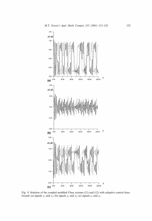
Fig. 9. Solution of the coupled modified Chua systems (11) and (12) with adaptive control deac-

tivated: (a) signals x1 and x2; (b) signals y1 and y2; (c) signals z1 and z2.


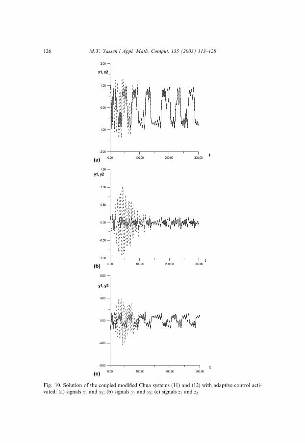
Fig. 10. Solution of the coupled modified Chua systems (11) and (12) with adaptive control acti-

vated: (a) signals x1 and x2; (b) signals y1 and y2; (c) signals z1 and z2.


activated at t ¼ 20: Fig. 5 shows that chaos is suppressed to limit cycle thatcontains the equilibrium point E0 for k1 ¼ 9:9152.

5.1.2. Adaptive control

Figs. 6–8 show the time response for the states x, y and z of the controlledsystem (2) after applying adaptive feedback control and the successful results

under the application of these adaptive control schemes.

5.2. Adaptive synchronization of two identical Chua circuits

Fourth-order Runge–Kutta method is used to solve the system of differentialequations (11), (12) associated with feedback control law (15) and the adaption

algorithm (16) with time step size 0.01. The results of the simulation of the two

identical modified Chua circuits without adaptive control are shown in Figs.

9(a)–(c). Figs. 10(a)–(c) show the states evolution of the derive system (11) and

the response system (12) after applying the feedback control (15) associated

with the adaption algorithm (16). The initial conditions of the error system (17)

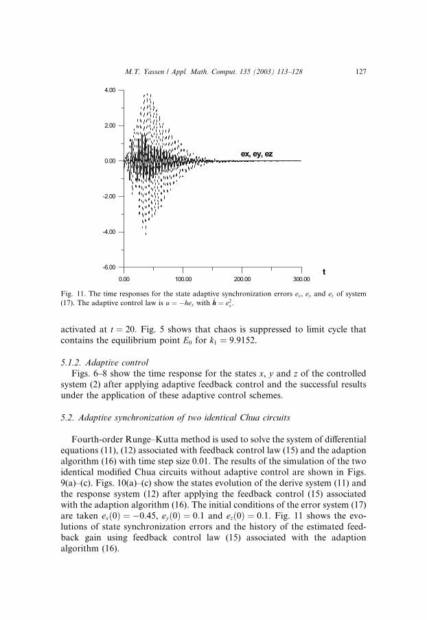
are taken exð0Þ ¼ �0:45, eyð0Þ ¼ 0:1 and ezð0Þ ¼ 0:1. Fig. 11 shows the evo-lutions of state synchronization errors and the history of the estimated feed-back gain using feedback control law (15) associated with the adaption

algorithm (16).

Fig. 11. The time responses for the state adaptive synchronization errors ex, ey and ez of system(17). The adaptive control law is u ¼ �hex with _hh ¼ e2x .


6. Conclusion

This work demonstrates that chaos in modified Chua’s circuit can be easily

controlled using adaptive control techniques.

References

[1] E. Ott, C. Grebogi, J.A. Yorke, Phys. Rev. Lett. 64 (11) (1990) 1196–1199.

[2] S. Rajasekar, K. Murali, M. Lakshmanan, Chaos, Soliton and Fractals 8 (9) (1997) 1545–1558.

[3] M. Ramesh, S. Narayanan, Chaos, Soliton and Fractals 10 (9) (1999) 1473–1489.

[4] G. Chen, X. Dong, IEEE Trans. Circuits and Systems 40 (9) (1993) 591–601.

[5] G. Chen, X. Dong, J. Circuits and Systems Comput. 3 (1) (1993) 139–149.

[6] G. Chen, in: IEEE Proc. of Amer. Contr. Conf., San Francisco, CA, 1993, pp. 2413–2414.

[7] G. Chen, Chaos, Soliton and Fractals 8 (9) (1997) 1461–1470.

[8] T.T. Hartley, F. Mossayebi, J. Circuits and Systems Comput. 3 (1993) 173–194.

[9] T. Saito, K. Mitsubori, IEEE Trans. Circuits and Systems 42 (1995) 168–172.

[10] C.C. Hwang, H.Y. Chow, Y.K. Wang, Physica D 92 (1996) 95–100.

[11] C.C. Hwang, J.Y. Hsieh, R.S. Lin, Chaos, Soliton and Fractals 8 (9) (1997) 1507–1515.

[12] K. Pyragas, Phys. Lett. A 170 (1992) 421–428.

[13] A. Hegazi, H.N. Agiza, M.M. El-Dessoky, Chaos, Soliton and Fractals 12 (2001) 631–658.

[14] L.M. Pecora, T.L. Carrol, Phys. Rev. Lett. 64 (8) (1990) 821–824.

[15] H.N. Agiza, M.T. Yassen, Phys. Lett. A 278 (2001) 191–197.

[16] T.L. Liao, S.H. Lin, J. Franklin Inst. 336 (1999) 925–937.

[17] E.W. Bai, K.E. Lonngren, Chaos, Soliton and Fractals 11 (2000) 1041–1044.

[18] M. di Bernardo, Phys. Lett. A 214 (1996) 139–144.

[19] R.N. Madan (Ed.), Chua’s Circuit, A Paradigm for Chaos, World Scientific, Singapore, 1993.

[20] C. Sparrow, The Lorenz Equations Bifurcation, Chaos and Strange Attractors, Springer, New

York, 1982.


adaptivecontrolandsynchronization ofamodiﬁedchua...

Documents