adaptive stochastic resonancesipi.usc.edu/~kosko/adaptivesr.pdf · adaptive stochastic resonance...

Adaptive Stochastic Resonance

SANYA MITAIM AND BART KOSKO, MEMBER, IEEE

This paper shows how adaptive systems can learn to add anoptimal amount of noise to some nonlinear feedback systems.Noise can improve the signal-to-noise ratio of many nonlineardynamical systems. This “stochastic resonance” (SR) effect occursin a wide range of physical and biological systems. The SReffect may also occur in engineering systems in signal processing,communications, and control. The noise energy can enhance thefaint periodic signals or faint broadband signals that force thedynamical systems. Most SR studies assume full knowledge ofa system’s dynamics and its noise and signal structure. Fuzzyand other adaptive systems can learn to induce SR based onlyon samples from the process. These samples can tune a fuzzysystem’s if–then rules so that the fuzzy system approximates thedynamical system and its noise response. The paper derives the SRoptimality conditions that any stochastic learning system shouldtry to achieve. The adaptive system learns the SR effect as thesystem performs a stochastic gradient ascent on the signal-to-noise ratio. The stochastic learning scheme does not depend ona fuzzy system or any other adaptive system. The learning processis slow and noisy and can require heavy computation. Robustnoise suppressors can improve the learning process when we canestimate the impulsiveness of the learning terms. Simulations testthis SR learning scheme on the popular quartic-bistable dynamicalsystem and on other dynamical systems. The driving noise typesrange from Gaussian white noise to impulsive noise to chaoticnoise. Simulations suggest that fuzzy techniques and perhaps otheradaptive “black box” or “intelligent” techniques can induce SRin many cases when users cannot state the exact form of thedynamical systems. The appendixes derive the basic additive fuzzysystem and the neural-like learning laws that tune it.

Keywords—Adaptive signal processing, dynamical systems,fuzzy systems, neural networks, noise processing, robust statistics,stochastic resonance.

I. STOCHASTIC RESONANCE AND ADAPTIVE

FUNCTION APPROXIMATION

Noise can sometimes enhance a signal as well as corruptit. This fact may seem at odds with almost a century ofeffort in signal processing to filter noise or to mask orcancel it. But noise is itself a signal and a free source ofenergy. Noise can amplify a faint signal in some feedbacknonlinear systems even though too much noise can swampthe signal. This implies that a system’s optimal noise levelneed not be zero noise. It also suggests that nonlinear signal

Manuscript received November 1, 1997; revised April 17, 1998.The authors are with the Signal and Image Processing Institute, Depart-

ment of Electrical Engineering, University of Southern California, LosAngeles, CA 90089-2564 USA.

Publisher Item Identifier S 0018-9219(98)07858-X.

systems with nonzero-noise optima may be the rule ratherthan the exception. Fig. 1 shows how uniform pixel noisecan improve our subjective perception of an image. A smalllevel of noise sharpens the image contours and helps fill infeatures. Too much noise swamps the image and degradesits contours.

Stochastic resonance(SR) [11]–[13], [21], [23], [26],[68], [80], [89], [128], [161], [162], [181], [185], [186],[193], [243] occurs when noise enhances an external forcingsignal in a nonlinear dynamical system. SR occurs in asignal system if and only if the system has a nonzeronoise optimum. The classic SR signature is a signal-to-noise ratio (SNR) that is not monotone. Fig. 2 shows theSR effect for the popular quartic-bistable dynamical system[13], [26], [179]. The SNR rises to a maximum and thenfalls as the variance of the additive white noise grows. Morecomplex systems may have multimodal SNR’s and so showstochastic “multiresonance” [79], [240].

SR holds promise for the design of engineering systemsin a wide range of applications. Engineers may want toshape the noise background of a fixed signal pattern toexploit the SR effect. Or they may want to adapt theirsignals to exploit a fixed noise background. Engineers nowadd noise to some systems to improve how humans perceivesignals. These systems include audio compact discs [150],analog-to-digital devices [10], video images [222], schemesfor visual perception [215], [216], [228], and cochlear im-plants [178], [182]. Some control and quantization schemesadd a noise-like dither to improve system performance [10],[147], [150], [198], [222]. Additive noise can sometimesstabilize chaotic attractors [16], [77], [168]. Noise can alsoimprove human tactile response [48], muscle contraction[42], and coordination [49]. This suggests that SR designsmay improve how robots grasp objects [51] or balancethemselves. SR designs might also improve how virtual oraugmented reality systems [32], [106] can create or enhancethe sensations of touch and balance.

SR designs might lead to better schemes to filter ormultiplex the faint signals found in spread spectrum com-munication systems [71], [227]. These systems transmit anddetect faint signals in noisy backgrounds across wide bandsof frequencies. SR designs might also exploit the signal-based crosstalk noise found in cellular systems [142], [229],Ethernet packet flows [143], or Internet congestion [113].

0018–9219/98$10.00 1998 IEEE

2152 PROCEEDINGS OF THE IEEE, VOL. 86, NO. 11, NOVEMBER 1998

(a) (b) (c) (d)

Fig. 1. Uniform pixel noise can improve the subjective response of our nonlinear perceptualsystem. The noise gives a nonmonotonic response: a small level of noise sharpens the image featureswhile too much noise degrades them. These noisy images result when we apply a pixel threshold tothe popular “Lena” image of signal processing [187]:y = g((x+n)��) whereg(x) = 1 if x � 0andg(x) = 0 if x < 0 for an input pixel valuex 2 [0; 1]and output pixel valuey 2 f0;1g. Theinput image’s gray-scale pixels vary from zero (black) to one (white). The threshold is� = 0:05.We threshold the original “Lena” image to give the faint image in (a). The uniform noisen has meanmn = �0:02 for images (b)–(d). The noise variance�2

ngrows from (b)–(d):�2

n= 1:67� 10�3

in (b), �2n

= 2:34 � 10�2 in (c), and�2n

= 1:67 � 10�1 in (d).

Fig. 2. The nonmonotonic signature of stochastic resonance. The graph shows the smoothed outputSNR of a quartic bistable system as a function of the standard deviation of additive white Gaussiannoisen. The vertical dashed lines show the absolute deviation between the smallest and largestoutliers in each sample average of 20 outcomes. The system has a nonzero noise optimum andthus shows the SR effect. The noisy signal-forced quartic bistable dynamical system has the form_x = f(x)+s(t)+n(t) = x�x3+" sin!0t+n(t). The Gaussian noisen(t) adds to the externalforcing narrowband signals(t) = " sin!0t. Other systems can use multiplicative noise [9], [27],[67], [74], [78], [83] or use non-Gaussian noise [36], [38], [39], [79], [206].

The study of SR has emerged largely from physics andbiology. The awkward term “stochastic resonance” stemsfrom a 1981 article in which physicists observed “thecooperative effect between internal mechanism and theexternal periodic forcing” in some nonlinear dynamical

systems [13]. Scientists soon explored SR in climatemodels [195] to explain how noise could induce periodicice ages [11], [12], [193], [194]. They conjectured thatglobal or other noise sources could amplify small periodicvariations in the Earth’s orbit. This might explain the

MITAIM AND KOSKO: ADAPTIVE STOCHASTIC RESONANCE 2153

observed 100 000 year primary cycle of the Earth’s iceages. This SR conjecture remains the subject of debate[73], [194], [245]. Physicists have since found strongerevidence of SR in ring lasers [170], [236], thresholdhysteretic Schmitt triggers [69], [171], Chua’s electricalcircuit [4], [5], bistable magnetic systems [97], electronparamagnetic resonance [81], [84], [217], magnetoelasticribbons [230], superconducting quantum interferencedevices (SQUID’s) [103], [117], [220], Ising systems [20],[188], [226], coupled diode resonators [151], tunnel diodes[165], [166], Josephson junctions [22], [104], opticalsystems [9], [61], [120], chemical systems [62], [72],[99], [105], [129], [145], [180], and quantum-mechanicalsystems [93]–[96], [153], [164], [205], [214], [235].

Some biological systems may have evolved to exploitthe SR effect. Most SR studies have searched for the SReffect in the sensory processing of prey and predators.Noisy or turbulent water can help the mechanoreceptorhair cells of the crayfishProcambarus clarkiidetect faintperiodic signals of predators such as a bass’s fin motion[58], [59], [186], [202], [208], [210], [243]. Noise helpsthe mechanosensors of the cricketAcheta domesticadetectsmall-amplitude low-frequency air signals from predators[146], [172], [173]. Dogfish sharks use noise in their mouthsensors when they detect periodic signals from prey [17].The SR effect appears in the mechanoreceptors in a rat’sskin [47] and in the neurons in a rat’s hippocampus [90].The SR effect occurs in a wide range of models of neurons[25], [27], [44], [45], [46], [102], [207], [231] and neuralnetworks [24], [25], [27], [29], [30], [41], [44]–[46], [114],[115], [149], [154]–[159], [183], [189], [206].

Research in SR has grown from the study of externalperiodic signals in simple dynamical systems to the study ofexternal aperiodic and broadband signals in more complexdynamical systems [35], [36], [41], [44]–[47], [102], [108],[146], [209], [231]. Below we review examples of thesedynamical systems and the performance measures involvedin the SR effect. There is no consensus on which signal-to-noise performance measure best measures the SR effect.The breadth of SR systems suggests that the SR effectmay occur in still more complex dynamical systems forstill more complex signals and noise types. These signalsystems may prove too complex to model with simpleclosed-form techniques. This suggests in turn that we mightuse “intelligent” or adaptive model-free techniques to learnor approximate the SR effects.

Below we explore how to learn the SR effect with adap-tive systems in general and with adaptive fuzzy functionapproximators [132]–[136] in particular. Adaptive fuzzysystems approximate functions with if–then rules that relatetunable fuzzy subsets of input and outputs. Each rule definesa fuzzy patch or subset of the input–output state space. Thefuzzy system approximates a function as its rule patchescover the graph of the function. These systems resemblethe radial-basis function networks found in neural networks[100], [176], [136]. Neural-like learning laws tune andmove the fuzzy rule patches as they tune the shape of thefuzzy sets that make up the rule patches. The learning laws

in the appendixes use input–output data from the samplednoisy dynamical system. The rule patches move quickly tocover optimal or near-optimal regions of the function (suchas its extrema). Experts can also state verbal if–then rules insome cases and add them to the fuzzy patch covering. Theserules offer a simple way to endow a fuzzy approximatorwith prior knowledge or “hints” [1], [2] that can improvehow well a fuzzy system approximates a function or howwell it generalizes from training samples [197]. Fuzzysystems achieve their patch-covering approximation at thehigh cost of rule explosion [135], [136]. The number ofrules grows exponentially with the state-space dimensionof the fuzzy system. We stress that our SR learning lawscan also tune nonfuzzy adaptive systems.

Adaptive fuzzy systems offer a balance between thestructured and symbolic rule-based expert systems foundin artificial intelligence [221] and the unstructured butnumeric approximators found in modern neural networks[100], [101], [132]. These or other adaptive model-freeapproximators might better model the SR effect in somedynamical systems. Our first goal was to show that adaptivesystems can learn to shape the input noise and perhapsshape other terms to achieve SR in the main closed-form dynamical systems that scientists have shown producethe SR effect. Our second goal was to suggest throughthese simulation experiments that adaptive fuzzy systems orother model-free approximators might achieve SR in morecomplex dynamical systems that defy easy math modelingor measurement.

This paper presents three main results. The first andcentral result is that a system can learn the SR effect ifit performs a stochastic gradient ascent on .Then the random noise gradient can tune theparameters in any adaptive system through a slow type ofstochastic approximation [219]. We derive these learninglaws in terms of discrete Fourier transforms. The ideabehind the gradient-ascent learning is that such hill climbingis nontrivial if and only if the SNR surface shows someform of SR. The second result is that the SNR first-ordercondition for an extremum has the ratio formfor . The term can produce impulsiveor even Cauchy noise that can destabilize the stochasticgradient ascent. Time lags in the training process cancompound this impulsiveness. The third result is that aCauchy-based noise suppressor from the theory of robuststatistics can often reduce the impulsiveness of the noisegradient and thus improve the learning process.

The paper reviews the main math models involved in SRto date and reviews the adaptive fuzzy rule structure thatcan implicitly approximate these models and produce a likeSR effect. The next two sections review these dynamicalsystems and the competing performance measures thatscientists have used to detect SR in them. We used astandard based on discrete Fourier spectra.Most SR research has focused on the quartic bistabledynamical system. We worked with that signal system indetail and also applied the stochastic learning scheme toother dynamical systems. The learning scheme converged


in most cases to the SR effect or the SNR mode in all ofthese systems. The SR learning scheme still converged forthe quartic bistable system when we replaced the forcingadditive Gaussian white noise with other additive randomnoise, with infinite-variance noise, and with chaotic noisefrom a chaotic logistic dynamical system. Sections V andVI derive the SR optimality conditions and the stochasticlearning law and then test the learning scheme in SR sim-ulations of the quartic bistable dynamical system and otherdynamical systems. The appendixes derive the supervisedlearning laws for the fuzzy function approximator wherethe fuzzy sets have the shape of sinc functions.

II. SR DYNAMICAL SYSTEMS

This section reviews the main known dynamical systemsthat show SR. These models involve only simple nonlin-earities. They also simply add a random noise term to adifferential equation rather than use a formal Ito stochasticdifferential [43], [60], [86]. There are so far no theoremsor formal taxonomies that tell which dynamical systemsshow SR and which do not. A dynamical system relatesits input–output response through a differential equation ofthe form

(1)

(2)

The input may depend on both time and on thesystem’s state . The system is unforced or autonomouswhen for all and . The system output ormeasurement depends on the state through .The output of a simple model neuron may be a signumfunction: .

A. Quartic Bistable System [13], [56], [75],[82], [109], [121], [179], [249]

The quartic bistable system is the most studied modelthat shows SR. It has the form

(3)

(4)

for a quartic potentialwith , input signal , and white Gaussiannoise with zero mean and varianceand . Researchers sometimes includethe forcing functions and in the potential function:

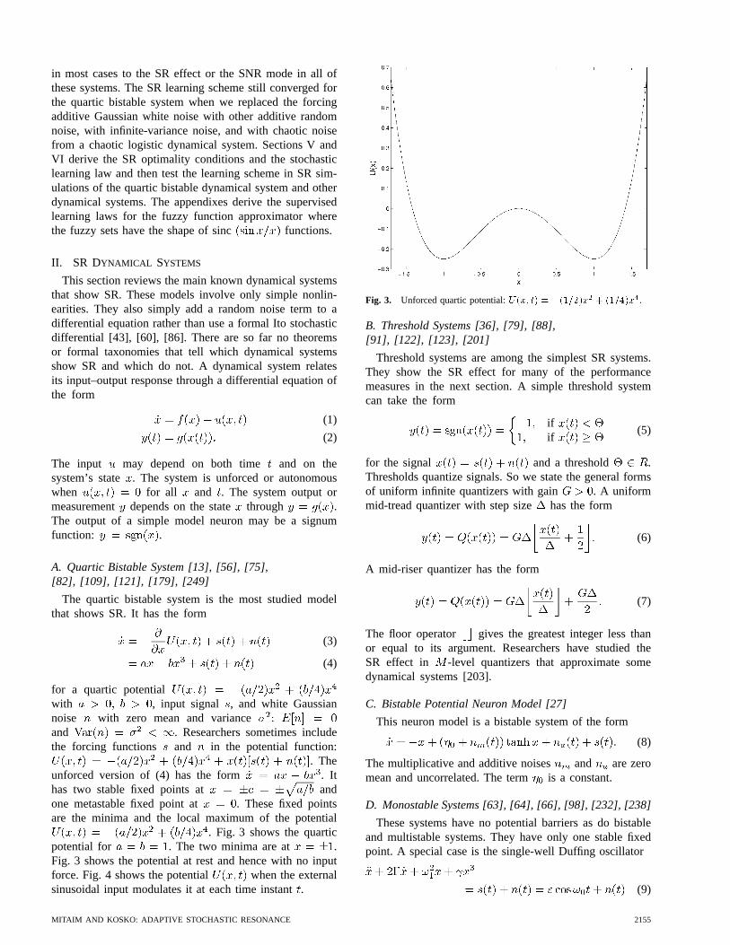
. Theunforced version of (4) has the form . Ithas two stable fixed points at andone metastable fixed point at . These fixed pointsare the minima and the local maximum of the potential

. Fig. 3 shows the quarticpotential for . The two minima are at .Fig. 3 shows the potential at rest and hence with no inputforce. Fig. 4 shows the potential when the externalsinusoidal input modulates it at each time instant.

Fig. 3. Unforced quartic potential:U(x; t) = �(1=2)x2 + (1=4)x4.

B. Threshold Systems [36], [79], [88],[91], [122], [123], [201]

Threshold systems are among the simplest SR systems.They show the SR effect for many of the performancemeasures in the next section. A simple threshold systemcan take the form

ifif

(5)

for the signal and a threshold .Thresholds quantize signals. So we state the general formsof uniform infinite quantizers with gain . A uniformmid-tread quantizer with step size has the form

(6)

A mid-riser quantizer has the form

(7)

The floor operator gives the greatest integer less thanor equal to its argument. Researchers have studied theSR effect in -level quantizers that approximate somedynamical systems [203].

C. Bistable Potential Neuron Model [27]

This neuron model is a bistable system of the form

(8)

The multiplicative and additive noises and are zeromean and uncorrelated. The term is a constant.

D. Monostable Systems [63], [64], [66], [98], [232], [238]

These systems have no potential barriers as do bistableand multistable systems. They have only one stable fixedpoint. A special case is the single-well Duffing oscillator

(9)


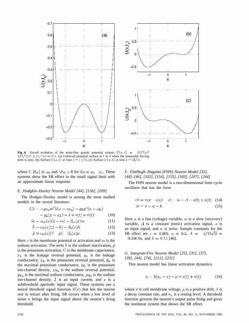
Fig. 4. Forced evolution of the noise-free quartic potential system:U(x; t) = �(1=2)x2

+(1=4)x4 + (1=4)x sin 2�t. (a) Unforced potential surface att = 0 when the sinusoidal forcingterm is zero. (b) SurfaceU(x; t) at time t = (1=4). (c) SurfaceU(x; t) at time t = (3=4).

where and for . Thesesystems show the SR effect in the small signal limit withan approximate linear response.

E. Hodgkin–Huxley Neuron Model [44], [156], [209]

The Hodgin–Huxley model is among the most studiedmodels in the neural literature.

(10)

(11)

(12)

(13)

Here is the membrane potential or activation andis thesodium activation. The term is the sodium inactivation,is the potassium activation, is the membrane capacitance,

is the leakage reversal potential, is the leakageconductance, is the potassium reversal potential, isthe maximal potassium conductance, is the potassiumion-channel density, is the sodium reversal potential,

is the maximal sodium conductance, is the sodiumion-channel density, is an input current, and is asubthreshold aperiodic input signal. These systems use aneural threshold signal function that lets the neuronrest or retract after firing. SR occurs when a low level ofnoise brings the input signal above the neuron’s firingthreshold.

F. FitzHugh–Nagumo (FHN) Neuron Model [35],[44]–[46], [102], [154], [155], [183], [207], [244]

The FHN neuron model is a two-dimensional limit cycleoscillator that has the form

(14)

(15)

Here is a fast (voltage) variable, is a slow (recovery)variable, is a constant (tonic) activation signal, isan input signal, and is noise. Sample constants for theSR effect are

, and [46].

G. Integrate-Fire Neuron Model [25], [31], [37],[39], [44], [74], [211], [231]

This neuron model has linear activation dynamics.

(16)

where is cell membrane voltage, is a positive drift, isa decay constant rate, and is a resting level. A thresholdfunction governs the neuron’s output pulse firing and givesthe nonlinear system that shows the SR effect.


H. Array And Coupled Systems [24], [27], [29],[30], [41], [44]–[46], [92], [110], [114],[115], [124], [149], [154]–[159], [177], [183],[188]–[190], [206], [212], [215], [216]

These systems combine many units of the above systems.They include neural networks and other coupled systems.A special case is the Cohen–Grossberg (“Hopfield”) [132]feedback neural network

for (17)

for neural activation potential , synaptic efficacy ,and hyperbolic neural firing function .Simulations show that the SR profile grows more peakedas the number of neurons grows [115]. One study [115]found that the SR effect goes away for .

I. Chaotic Systems [3], [5], [13], [33], [52],[160], [196], [241], [242], [251]

Some chaotic systems show the SR effect. These modelsinclude Chua’s electric circuit, the Henon map, the Lorenzsystem, and the following forced Duffing oscillator:

(18)

At least one researcher [87] has argued that noise-inducedchaos-order transitions need not be SR.

J. Random Systems [15], [19], [28], [68], [144], [252]

These systems include many classical random processessuch as random walks and Poisson processes. They alsoinclude the pulse system [15] whose response is a randomtrain of pulses with a pulse probability that depends onan input signal through

(19)

The input is the signal plus noise:. This model includes many -driven physiochemical

systems [15].Other systems show SR in the literature [7], [11], [14],

[20], [55], [107], [127], [167], [169], [188], [193], [213],[225], [239], [246], [248]. Special issues of physics journals[23], [181] also present other systems that show SR. Mostuse the SR measures in the next section.

III. SR PERFORMANCE MEASURES

This section reviews the most popular measures of SR.These performance measures depend on the forcing signaland noise and can vary from system to system. There isno consensus in the SR literature on how to measure theSR effect.

Some researchers study a stochastic dynamical systemin terms of the Fokker–Planck (or forward Kolmogorov)equation [57], [125], [184], [218]

(20)

for drift term and diffusion term . This partialdifferential equation stems from a Taylor series and showshow a probability density function of a Markov system’sstates evolves in time. System nonlinearities often precludeclosed-form solutions. Approximations and assumptionssuch as small noise and small signal effects can give closed-form solutions in some cases. These solutions motivatesome of the performance measures below. SR dynamicalsystems in general need not be Markov processes [78],[192].

A. Signal-to-Noise Ratio

The most common SR measure is some form of SNR[69], [75], [85], [111], [169], [249]. This seems the mostintuitive measure, even though there are many ways todefine SNR.

Suppose the input signal is the sinewave .Then the SNR measures how much the system output

contains the input signal frequency

(21)

dB (22)

The signal power is the magnitude of theoutput power spectrum at the input frequency .The background noise spectrum at input frequency

is some average of at nearby frequencies [116],[169], [249]. The discrete Fourier transform (DFT)for is an exponentially weighted sum ofelements of a discrete-time sequence ofoutput signal samples

(23)

The signal frequency corresponds to bin in the DFTfor integer and for . This gives theoutput signal in terms of a DFT as . The noisepower is the average power in the adjacent bins

for some integer[6], [249]

(24)

We expand this noise term in Section V to include allenergy not due to the signal.

An adiabatic approximation [169] can give an explicitSNR for the quartic bistable system in (4) with sinewaveinput

(25)

(26)


(a) (b)

(c)

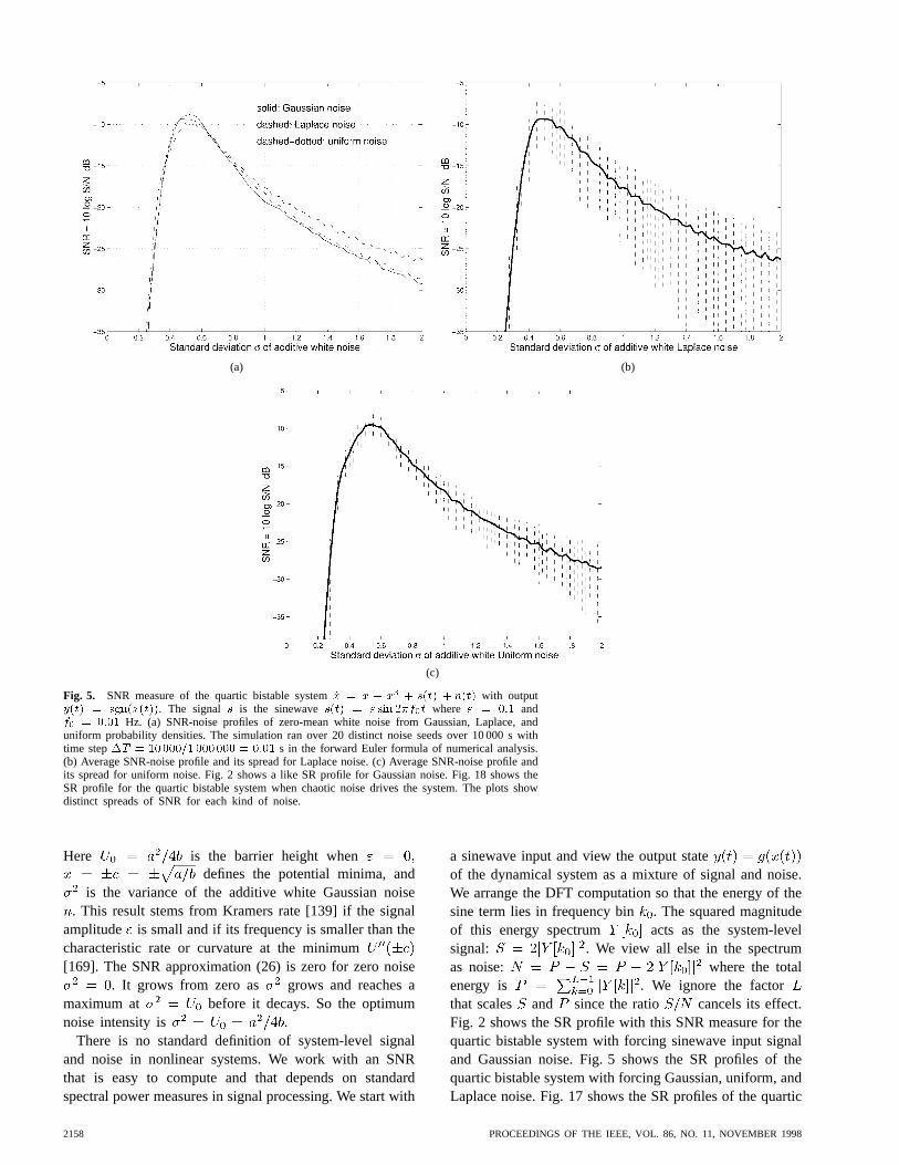
Fig. 5. SNR measure of the quartic bistable system_x = x � x3 + s(t) +n(t) with outputy(t) = sgn(x(t)). The signals is the sinewaves(t) = " sin 2�f0t where " = 0:1 andf0 = 0:01 Hz. (a) SNR-noise profiles of zero-mean white noise from Gaussian, Laplace, anduniform probability densities. The simulation ran over 20 distinct noise seeds over 10 000 s withtime step�T = 10000=1000000 = 0:01 s in the forward Euler formula of numerical analysis.(b) Average SNR-noise profile and its spread for Laplace noise. (c) Average SNR-noise profile andits spread for uniform noise. Fig. 2 shows a like SR profile for Gaussian noise. Fig. 18 shows theSR profile for the quartic bistable system when chaotic noise drives the system. The plots showdistinct spreads of SNR for each kind of noise.

Here is the barrier height whendefines the potential minima, and

is the variance of the additive white Gaussian noise. This result stems from Kramers rate [139] if the signal

amplitude is small and if its frequency is smaller than thecharacteristic rate or curvature at the minimum[169]. The SNR approximation (26) is zero for zero noise

. It grows from zero as grows and reaches amaximum at before it decays. So the optimumnoise intensity is .

There is no standard definition of system-level signaland noise in nonlinear systems. We work with an SNRthat is easy to compute and that depends on standardspectral power measures in signal processing. We start with

a sinewave input and view the output stateof the dynamical system as a mixture of signal and noise.We arrange the DFT computation so that the energy of thesine term lies in frequency bin . The squared magnitudeof this energy spectrum acts as the system-levelsignal: . We view all else in the spectrumas noise: where the totalenergy is . We ignore the factorthat scales and since the ratio cancels its effect.Fig. 2 shows the SR profile with this SNR measure for thequartic bistable system with forcing sinewave input signaland Gaussian noise. Fig. 5 shows the SR profiles of thequartic bistable system with forcing Gaussian, uniform, andLaplace noise. Fig. 17 shows the SR profiles of the quartic


(a)

(b)

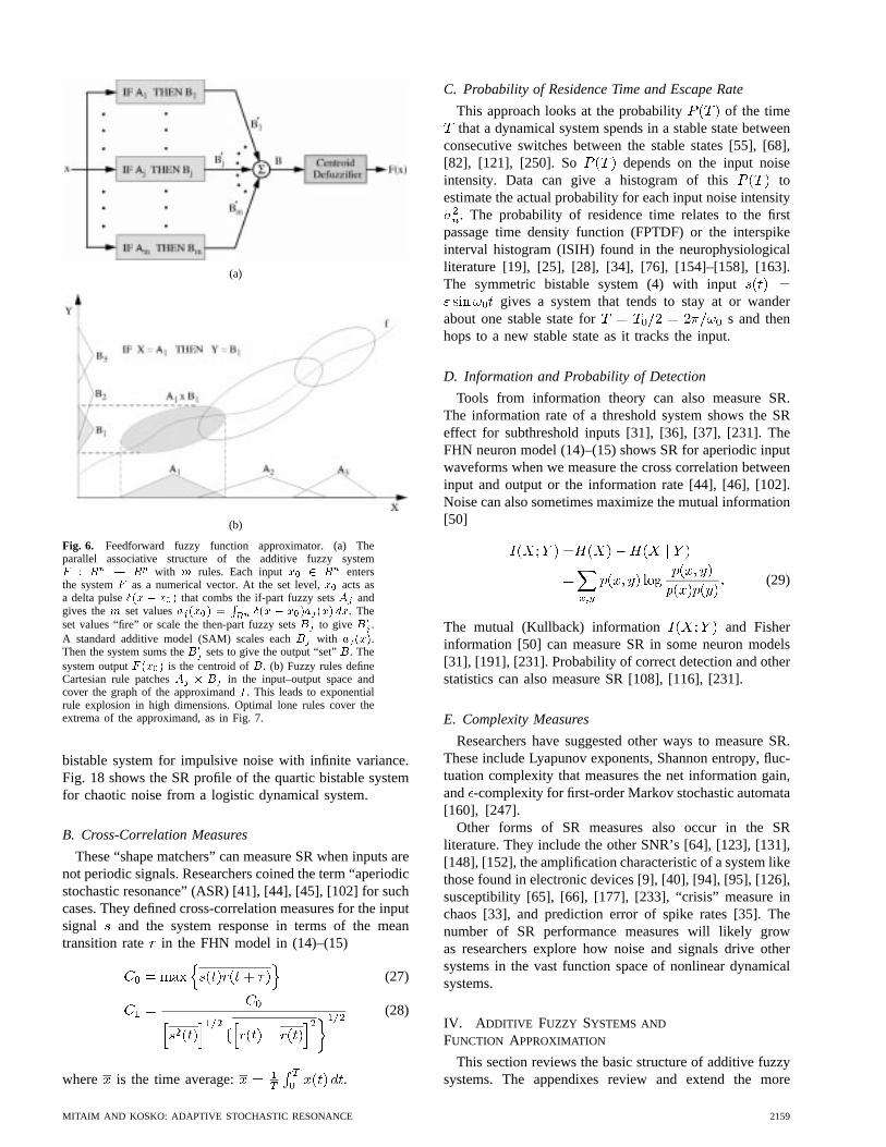
Fig. 6. Feedforward fuzzy function approximator. (a) Theparallel associative structure of the additive fuzzy systemF : Rn ! Rp with m rules. Each inputx0 2 Rn entersthe systemF as a numerical vector. At the set level,x0 acts asa delta pulse�(x � x0) that combs the if-part fuzzy setsAj andgives them set valuesaj(x0) =

R�(x � x0)aj(x) dx. The

set values “fire” or scale the then-part fuzzy setsBj to giveB0

j .A standard additive model (SAM) scales eachBj with aj(x).Then the system sums theB0

j sets to give the output “set”B. Thesystem outputF (x0) is the centroid ofB. (b) Fuzzy rules defineCartesian rule patchesAj � Bj in the input–output space andcover the graph of the approximandf . This leads to exponentialrule explosion in high dimensions. Optimal lone rules cover theextrema of the approximand, as in Fig. 7.

bistable system for impulsive noise with infinite variance.Fig. 18 shows the SR profile of the quartic bistable systemfor chaotic noise from a logistic dynamical system.

B. Cross-Correlation Measures

These “shape matchers” can measure SR when inputs arenot periodic signals. Researchers coined the term “aperiodicstochastic resonance” (ASR) [41], [44], [45], [102] for suchcases. They defined cross-correlation measures for the inputsignal and the system response in terms of the meantransition rate in the FHN model in (14)–(15)

(27)

(28)

where is the time average: .

C. Probability of Residence Time and Escape Rate

This approach looks at the probability of the timethat a dynamical system spends in a stable state between

consecutive switches between the stable states [55], [68],[82], [121], [250]. So depends on the input noiseintensity. Data can give a histogram of this toestimate the actual probability for each input noise intensity

. The probability of residence time relates to the firstpassage time density function (FPTDF) or the interspikeinterval histogram (ISIH) found in the neurophysiologicalliterature [19], [25], [28], [34], [76], [154]–[158], [163].The symmetric bistable system (4) with input

gives a system that tends to stay at or wanderabout one stable state for s and thenhops to a new stable state as it tracks the input.

D. Information and Probability of Detection

Tools from information theory can also measure SR.The information rate of a threshold system shows the SReffect for subthreshold inputs [31], [36], [37], [231]. TheFHN neuron model (14)–(15) shows SR for aperiodic inputwaveforms when we measure the cross correlation betweeninput and output or the information rate [44], [46], [102].Noise can also sometimes maximize the mutual information[50]

(29)

The mutual (Kullback) information and Fisherinformation [50] can measure SR in some neuron models[31], [191], [231]. Probability of correct detection and otherstatistics can also measure SR [108], [116], [231].

E. Complexity Measures

Researchers have suggested other ways to measure SR.These include Lyapunov exponents, Shannon entropy, fluc-tuation complexity that measures the net information gain,and -complexity for first-order Markov stochastic automata[160], [247].

Other forms of SR measures also occur in the SRliterature. They include the other SNR’s [64], [123], [131],[148], [152], the amplification characteristic of a system likethose found in electronic devices [9], [40], [94], [95], [126],susceptibility [65], [66], [177], [233], “crisis” measure inchaos [33], and prediction error of spike rates [35]. Thenumber of SR performance measures will likely growas researchers explore how noise and signals drive othersystems in the vast function space of nonlinear dynamicalsystems.

IV. A DDITIVE FUZZY SYSTEMS AND

FUNCTION APPROXIMATION

This section reviews the basic structure of additive fuzzysystems. The appendixes review and extend the more


Fig. 7. Lone optimal fuzzy rule patches cover the extrema ofapproximandf . A lone rule defines a flat line segment that cuts thegraph of the local extremum in at least two places. The mean valuetheorem implies that the extremum lies between these points. Thiscan reduce much of fuzzy function approximation to the search forzeroesx of the derivative mapf 0 : f 0(x) = 0.

formal math structure that underlies these adaptive functionapproximators.

A fuzzy system stores rules of the wordform “If Then ” or the patch form

. The if-part fuzzy setsand then-part fuzzy sets have set functions

and . Generalized fuzzy setsmap to intervals other than . The scalar sinc set func-tions in Fig. 23 map real inputs to “membership degrees”in the bipolar range . The system design musttake care when these negative set values enter the SAMratio in (31). The system can use the joint set functionor some factored form such asor , or any other con-junctive form for input vector[132].

An additive fuzzy system [132], [133] sums the “fired”then-part sets

(30)

Fig. 6(a) shows the parallel fire-and-sum structure of theSAM. These nonlinear systems can uniformly approximateany continuous (or bounded measurable) functionon acompact domain [133], [136]. Engineers often apply fuzzysystems to problems of control [119] but fuzzy systems canalso apply to problems of communication [200] and signalprocessing [130] and other fields.

Fig. 6(b) shows how three rule patches can cover part ofthe graph of a scalar function . The patch-coverstructure implies that fuzzy systems sufferfrom rule explosionin high dimensions. A fuzzy system

needs on the order of rules to cover the graphand thus to approximate a vector function .Optimal rules can help deal with the exponential ruleexplosion. Lone or local mean-squared optimal rule patchescover the extrema of the approximand[135], [136]. They“patch the bumps” as in Fig. 7. Better learning schemesmove rule patches to or near extrema and then fill inbetween extrema with extra rule patches if the rule budgetallows.

The scaling choice gives a SAM. Appen-dix A shows that taking the centroid of in (30) givesthe following SAM ratio [132], [133], [134], [135]:

(31)

Here is the finite positive volume or area of then-part setand is the centroid of or its center of mass. The

convex weights have the form. The convex coefficients

change with each input vector.Fig. 8 shows how supervised learning moves and shapes

the fuzzy rule patches to give a finer approximation asthe system samples more input–output data. Appendix Bderives the supervised SAM learning algorithms for the sincset functions [136], [174], [175] in Fig. 23 that we use inthe SR simulations. Supervised gradient ascent changes theSAM parameters with performance data. The learning lawsupdate each SAM parameter to maximize the performancemeasure of the SR dynamical system. This processrepeats as needed for a large number of sample data pairs

. Fig. 8(e) displays the absolute error of the sinc-based fuzzy function approximation.

V. SR LEARNING AND EQUILIBRIUM

The scalar SAM fuzzy system can learnthe SR pattern of optimum noise of an unknown dynamicalsystem if it uses enough rules and if it samples enoughdata from a dynamical system that stochastically resonates.Below we derive a gradient-based learning law that tunesthe SAM parameters to achieve SR from samples of systemdynamics. It can also tune the parameters in other adaptivesystems. We first define a practical SNR measure in termsof discrete Fourier transforms. Other SR measures can giveother learning laws.

A. The SNR in Nonlinear Systems

Suppose a nonlinear dynamical system has a sinewaveforcing function of known frequency Hz. We searchthe sinusoidal part of the output for the knownfrequency but unknown amplitude and phase in thesystem output response . The “noisy signal” hasthe form of “signal” plus “noise”

(32)

The SNR at the output is the spectral ratio of the energy ofto the energy of . We assume that the signal

is always present. This ignores the important problem ofsignal detection but lets us focus on learning the SR effect.

We define the SNR measure as

(33)

Here , and is the-point discrete Fourier transform (DFT) of

(34)


Fig. 8. Fuzzy function approximation. Two-dimensional (2-D) sinc SAM function approximationwith 100 fuzzy if–then rules and supervised gradient descent learning. (a) Desired function orapproximandf . (b) SAM initial phase as a flat sheet or constant approximatorF . (c) SAMapproximatorF after it initializes its centroids to the samples:cj = f(mj). (d) SAM approximatorF after 100 epochs of learning. (e) SAM approximatorFafter 6000 epochs of learning. (f) Absoluteerror of the fuzzy function approximation(jf � F j).

We assume that the discrete frequency isan integer for sampling rate and . We alsoassume that there is no aliasing due to sampling. Then wecan show that for large the SNR measure in (33) tendsto the standard definition of SNR as a ratio of variances.

Theorem:

(35)

Here and. We need further assumptions to derive

(35). First consider the “energy” in each frequency binof the transform

(36)

(37)

(38)

(39)

where and are the DFT’s of and in (32).Suppose the sinusoidal term has the form

(40)

for . Its DFT has the form [199]

(41)

(42)

(43)

(44)

where is an integer, isa frequency band, , and is the Kroneckerdelta function. So vanishes when both and

. This gives

(45)

So and contain all the energy of thesinusoidal signal . We define the noise power as

and assume that is stationary and ergodic withzero mean. Then Parseval’s theorem gives

(46)

(47)

(48)


The ergodicity of gives (47). Now consider the totaloutput spectrum

(49)

(50)

(51)

(52)

(53)

Then (53) and (39) give

(54)

Then the SNR structure in (33) follows:

(55)

(56)

(57)

for large and for small (or null) and .Note that for due to thesymmetry of the DFT.

The result (57) also holds if the zero-mean noise sequenceis not correlated in time and does not correlate with

. Then we can take expectations of andto get

(58)

(59)

(60)

(61)

(62)

(63)

(64)

and

(65)

(66)

(67)

Putting (64) and (67) into (33) gives

(68)

(69)

Then as .

B. Supervised Gradient Learning and SR Optimality

An adaptive system can learn an SR noise pattern thatmaximizes a dynamical system’s SNR. The learning lawupdates a parameter of a SAM fuzzy system (or of anyother adaptive system) at time stepwith the deterministiclaw

(70)

for learning coefficients . This is gradient ascentlearning. We assume that the first-order moment of the SNRexists. We seldom know the probability structure or theexpectation of the SNR. So we estimate this expectationwith its random realization at each time step:

. This gives thestochasticgradient learning law

(71)

or simple random hill climbing. We assume the chain ruleholds (at least approximately) to give

(72)

Here is the noise level or standard deviation of the forcingnoise term . We want the SAM or other adaptive system

to approximate the optimum noise levelfor any inputsignal or initial condition of the dynamical system: .We then use and interchangeably

(73)

The term shows how any adaptive systemdepends on its th parameter . We again assume that


the chain rule holds to get

(74)

Then implies that

(75)

(76)

Like results hold for the decibel definitiondB for the base-10 logarithm

(77)

(78)

We next put (75)–(78) into (74) to get the log term thatdrives SR learning

ifif

(79)

The right side of (79) leads to the first-order condition foran SNR extremum

(80)

or simply

(81)

We can rewrite this optimality condition as

(82)

when the partial derivatives of and with respect toare not zero at . Equations (80) and (82) give anecessary condition for the SR maximum. The result (82)says that at SR the ratio of the rate of changes ofandmust equal the ratio of and . This has the same formas the result in microeconomics [140] that the marginalrates of substitution of two goods must at optimality equalthe partial derivatives of the utility function with respectto each good. But (81) and (82) hold only in a stochasticsense for sufficiently well-behaved random processes.

We find the second-order condition for an SR maximumwhen from

(83)

(84)

(85)

(86)

(87)

or . The last equality follows from thefirst-order condition or

since then . A likeresult holds for . We still get the second-ordercondition

(88)

These first- and second-order conditions show how thesignal power and noise power relate to each otherand to their derivatives at the SR maximum.

Much of the noisiness and complexity of the randomlearning law (71) stems from the probability structure thatunderlies the random optimality “error” process

(89)

near the optimum noise . The probability densityof depends on the statistics of the input noise, thedifferential equation that defines the dynamical system, andhow we define the signal and noise termsand .

Below we test statistics of the random processfor thequartic bistable system in Fig. 9. The results suggest that insome cases the density ofis Cauchy or otherwise belongsto the “impulsive” or thick-tailed family of symmetricalpha-stable bell curves with parameterin the characteris-tic function [18], [70], [223], [224]. The parameterlies in and gives the Gaussian random variablewhen or . It gives the thicker-tailedCauchy bell curve when or . Themoments of stable distributions with are finite onlyup to the order for . The Gaussian density alone hasfinite variance and higher moments. Alpha-stable randomvariables characterize the class of normalized sums thatconverge in distribution to a random variable [18] as in thefamous Gaussian version of the central limit theorem. Thenoisiness or impulsiveness of the-based learning growsas falls. Note also that the ratio is Cauchy ifand are jointly Gaussian [70], [137], [141], [204]. Oursimulations found that the impulsiveness ofstemmed atleast in part from the step size of the successive DFT’s in(92).

We now derive the SR learning laws in terms of DFT’s.We can approximate and with a ratio oftime differences at each iteration

(90)

(91)


The math model in (1)–(2) gives the exact learning laws.Recall that the -point DFT [199] for a sequence of states

has the form

(92)

The time index denotes the current time forthe sampling period . Let denote the partialderivative of the signal energy at iteration with respectto the output evaluated at time step:

. We likewise put and. We assume some form of the chain

rule holds to give

and

(93)

We first derive and in (93). Considerthe partial derivative of with respect to at timestep

(94)

(95)

(96)

(97)

(98)

So the partial derivative of the signal spectrumis

(99)

The partial derivative follows in like manner

(100)

(101)

from Parseval’s relation

(102)

(103)

We can consider the term in (93) as a sample ofat the time step .

Recall the math model of the dynamical system (1)–(2)and let . Assume that

for the zero-mean white noiseprocess with unit variance . So the modelbecomes

(104)

(105)

The chain rule gives

(106)

Let denote . Assume that is sufficientlydifferentiable. Then differentiate with respect to time [8]to get

(107)

(108)

The last derivative results from ’s explicit depen-dence on . So the additive case

gives

(109)

(110)

We need to simulate the evolution (108) for andobtain from (106). Then we put (99), (103), andinto (93) to get the stochastic gradient learning law

(111)

(112)

(113)

Here we omit the constant factor from (75)–(78) orview it as part of the learning rate in (113). The learninglaw for the parameters of a function approximator

that approximates the surface of optimal noise levelsfollows in like manner. Here replaces the parameterso the learning law becomes

(114)

(115)


(I) (II)

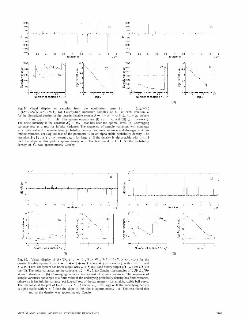
Fig. 9. Visual display of samples from the equilibrium termEn = (Sn=Nn)� ((@Sn=@�)=(@Nn=@�)). (a) Cauchy-like impulsive samples ofEn at each iterationnfor the discretized version of the quartic bistable system_x = x � x3 + " sin 2�f0t + n(t)where" = 0:1 and f0 = 0:01 Hz. The system outputs are (I)yt = xt and (II) yt = sgn(xt).The noise intensity is the constant�2

n= 0:25 that lies near the optimal level. (b) Converging

variance test as a test for infinite variance. The sequence of sample variances will convergeto a finite value if the underlying probability density has finite variance and diverges if it hasinfinite variance. (c) Log-tail test of the parameter� in an alpha-stable probability density. Thetest plotslogProb(X > u) versuslogu for largeu. If the density is alpha-stable with� < 2then the slope of this plot is approximately��. The test found� � 1. So the probabilitydensity of En was approximately Cauchy.

(I) (II)

Fig. 10. Visual display of @ SNRn=@� = (1=Sn)(@Sn=@�) �(1=Nn)(@Nn=@�) for thequartic bistable system_x = x � x3 +s(t) + n(t) where s(t) = " sin 2�f with " = 0:1 andf = 0:01Hz. The system has linear outputy(t) = x(t) in (I) and binary outputy(t) = sgn(x(t)) inthe (II). The noise variances are the constants�2

n= 0:25. (a) Cauchy-like samples of@ SNRn=@�

at each iterationn. (b) Converging variance test as test of infinite variance. The sequence ofsample variances converges to a finite value if the underlying probability density has finite variance,otherwise it has infinite variance. (c) Log-tail test of the parameter� for an alpha-stable bell curve.The test looks at the plot oflogProb(X > u) versuslogu for largeu. If the underlying densityis alpha-stable with� < 2 then the slope of this plot is approximately��. This test found that� � 1 and so the density was approximately Cauchy.


(a) (b)

Fig. 11. Learning paths for the quartic bistable system with output (a)y(t) = x(t) and (b)y(t) = sgn(x(t)). The learning law takes the form (113). The optimal noise level is� � 0:5 forboth cases. The impulsiveness of the learning term@ SNR=@� destabilizes the learning processnear the optimal noise level.

(a) (b)

Fig. 12. Learning paths for the quartic bistable system with outputy(t) = x(t). The learninglaw has the form (132). Optimal noise levels are (a)� � 0:35 and (b)� � 0:5. The learningpaths converge close to the optimal levels.

(116)

We get (113) if replaces and . Appendix B de-rives the last partial derivative in the chain-ruleexpansion (73) for all SAM fuzzy parameters . Thisis again the step where users can insert other adaptivefunction approximators and derive learning laws for theirparameters by expanding . Formal stochasticapproximation [219] further requires that the learning rate

must decrease slowly but not too slowly

and (117)

Linear decay terms obey (117). We used smallbut constant learning rates in most simulations.

VI. SR LEARNING: SIMULATION RESULTS

This section shows how the stochastic SR learning lawsin Section V tend to find the optimal noise levels in manydynamical systems. The learning process updates the noiseparameter at each iteration . The learning processis noisy and may not be stable due to the impulsivenessof the random gradient . We used a Cauchy


(a) (b)

Fig. 13. Impulsive effects on learning paths of noise intensity�n. The quartic bistable system hasthe form _x = x � x3 + s(t) + n(t) with binary outputy(t) = sgn(x(t)) and initial conditionx(0) = �1. The input sinusoid signal function iss(t) = 0:1 sin 2�(0:01)t. (a) The sequence�nwith different initial values that differ from the optimum noise intensity. (b) Noise-SNR profile ofthe quartic bistable system. The graph shows that the optimum noise intensity lies near� = 0:5.The paths of�n do not converge to the optimum noise. This stems from the impulsiveness of thederivative term@ SNRn=@� in the approximate SR learning law (137).

noise suppressor from the theory of robust statistics [112]to stabilize the learning process. Then sample paths ofconverged and wander about the optimal values if the initialvalues were close to the optimum.

The response of a system depends on its dynamics andon the nature of its input signals. We applied the SNRmeasure to the quartic bistable and other dynamical systemswith sinusoidal inputs. Future research may extend SRlearning to wideband input signals. Fig. 24(a) shows howthe optimum noise level varies for each input sinewave inthe quartic bistable system. The learning process samplesthe system’s input–output response as it learns the optimumnoise. It does not make direct use of the equation thatunderlies the system.

An adaptive fuzzy system can encode this pattern ofoptimum noise in its if–then rules when gradient learningtunes its parameters. The fuzzy system learns this optimumnoise level as it varies the output of a random noisegenerator. More complex fuzzy systems can themselves actas adaptive random number generators [136], [200].

Consider the forced dynamical system in (1)–(2) withinitial condition . We set up a discrete computersimulation with the stochastic version of Euler’s method(the Euler–Maruyama scheme) [53], [86], [115]

(118)

(119)

with initial condition . Here the zero-meanwhite noise sequence has unit variance . Theterm scales so that conforms with theWiener increment [86], [115], [184]. The learning processitself does not use the system model in any calculation. Itneeds access only to the system’s input–output responses.The learning process’s sampling period differs from

Fig. 14. Visual display of sample statistics of approximated@ SNRn=@�. (a) Cauchy-like samples of@ SNRn=@� ateach iterationn for quartic bistable system with sinusoidalinput of amplitude " = 0:1 and frequencyf0 = 0:01Hz. We compute @ SNRn=@� at each iteration from@ SNRn=@� � [(Sn � Sn�1)=Sn � (Nn �Nn�1)=Nn]sgn(�n � �n�1) in (136). We vary the noise level�n between�n = 0:50 and �n = 0:51 so thatsgn(�n � �n�1) changesvalues between 1 and�1. The plot shows impulsiveness ofthe random variable@ SNRn=@�. (b) Converging variance testas test of infinite variance. The sequence of sample variancesconverges to a finite value if the underlying probability densityhas finite variance. Else it has infinite variance. (c) Log-tail testof the parameter� in for an alpha-stable bell curve. The testlooks at the plot oflogProb(X > u) versus logu for largeu. If the underlying density is alpha-stable with� < 2 thenthe slope of this plot is approximately��. This test found that� � 1 and so the density was approximately Cauchy. The resultis that we need to apply the Cauchy noise suppressor (131) tothe approximate SR gradient@ SNRn=@� in (136) as well as tothe exact SR gradient in (129).

the time step of the dynamical system’s simulator in(118)–(119). The subsampling rate for the quartic bistablesystem is 1 : 50. We ignored all aliasing effects.


(a) (b)

(c) (d)

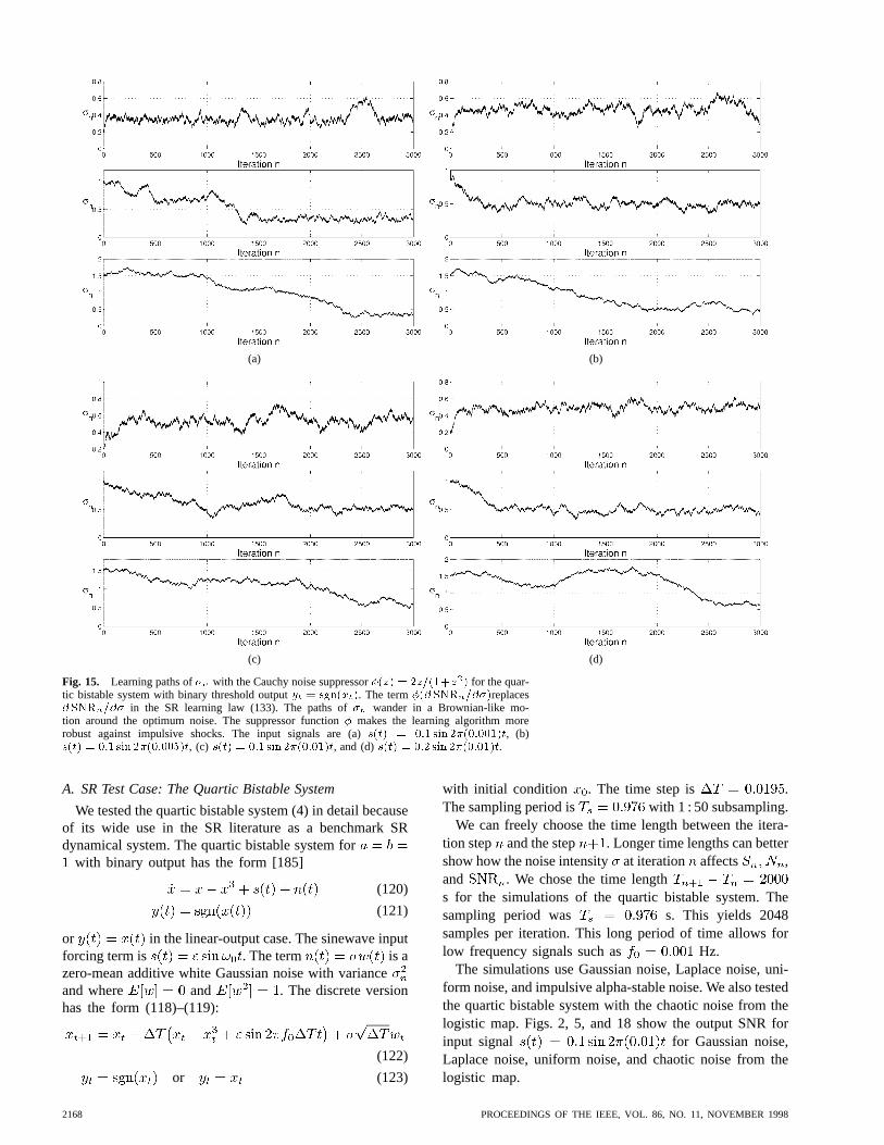
Fig. 15. Learning paths of�n with the Cauchy noise suppressor�(z) = 2z=(1+z2) for the quar-tic bistable system with binary threshold outputyt = sgn(xt). The term�(@ SNRn=@�)replaces@ SNRn=@� in the SR learning law (133). The paths of�n wander in a Brownian-like mo-tion around the optimum noise. The suppressor function� makes the learning algorithm morerobust against impulsive shocks. The input signals are (a)s(t) = 0:1 sin 2�(0:001)t, (b)s(t) = 0:1 sin 2�(0:005)t, (c) s(t) = 0:1 sin 2�(0:01)t, and (d)s(t) = 0:2 sin 2�(0:01)t.

A. SR Test Case: The Quartic Bistable System

We tested the quartic bistable system (4) in detail becauseof its wide use in the SR literature as a benchmark SRdynamical system. The quartic bistable system for

with binary output has the form [185]

(120)

(121)

or in the linear-output case. The sinewave inputforcing term is . The term is azero-mean additive white Gaussian noise with varianceand where and . The discrete versionhas the form (118)–(119):

(122)

or (123)

with initial condition . The time step is .The sampling period is with 1 : 50 subsampling.

We can freely choose the time length between the itera-tion step and the step . Longer time lengths can bettershow how the noise intensityat iteration affects ,and . We chose the time lengths for the simulations of the quartic bistable system. Thesampling period was s. This yields 2048samples per iteration. This long period of time allows forlow frequency signals such as Hz.

The simulations use Gaussian noise, Laplace noise, uni-form noise, and impulsive alpha-stable noise. We also testedthe quartic bistable system with the chaotic noise from thelogistic map. Figs. 2, 5, and 18 show the output SNR forinput signal for Gaussian noise,Laplace noise, uniform noise, and chaotic noise from thelogistic map.


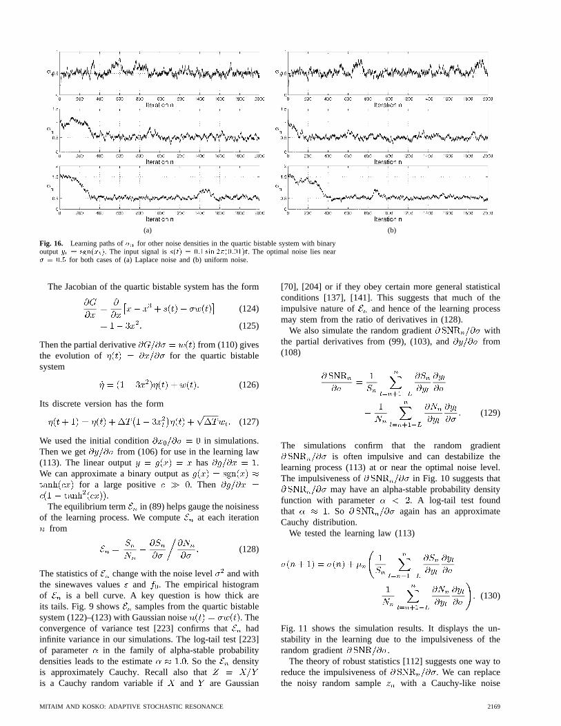
(a) (b)

Fig. 16. Learning paths of�n for other noise densities in the quartic bistable system with binaryoutput yt = sgn(xt). The input signal iss(t) = 0:1 sin 2�(0:01)t. The optimal noise lies near� = 0:5 for both cases of (a) Laplace noise and (b) uniform noise.

The Jacobian of the quartic bistable system has the form

(124)

(125)

Then the partial derivative from (110) givesthe evolution of for the quartic bistablesystem

(126)

Its discrete version has the form

(127)

We used the initial condition in simulations.Then we get from (106) for use in the learning law(113). The linear output has .We can approximate a binary output as

for a large positive . Then.

The equilibrium term in (89) helps gauge the noisinessof the learning process. We compute at each iteration

from

(128)

The statistics of change with the noise level and withthe sinewaves values and . The empirical histogramof is a bell curve. A key question is how thick areits tails. Fig. 9 shows samples from the quartic bistablesystem (122)–(123) with Gaussian noise . Theconvergence of variance test [223] confirms that hadinfinite variance in our simulations. The log-tail test [223]of parameter in the family of alpha-stable probabilitydensities leads to the estimate . So the densityis approximately Cauchy. Recall also thatis a Cauchy random variable if and are Gaussian

[70], [204] or if they obey certain more general statisticalconditions [137], [141]. This suggests that much of theimpulsive nature of and hence of the learning processmay stem from the ratio of derivatives in (128).

We also simulate the random gradient withthe partial derivatives from (99), (103), and from(108)

(129)

The simulations confirm that the random gradientis often impulsive and can destabilize the

learning process (113) at or near the optimal noise level.The impulsiveness of in Fig. 10 suggests that

may have an alpha-stable probability densityfunction with parameter . A log-tail test foundthat . So again has an approximateCauchy distribution.

We tested the learning law (113)

(130)

Fig. 11 shows the simulation results. It displays the un-stability in the learning due to the impulsiveness of therandom gradient .

The theory of robust statistics [112] suggests one way toreduce the impulsiveness of . We can replacethe noisy random sample with a Cauchy-like noise


(a)

(b)

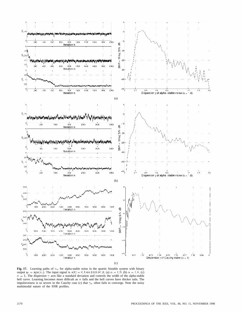
(c)

Fig. 17. Learning paths of n for alpha-stable noise in the quartic bistable system with binaryoutputyt = sgn(xt). The input signal iss(t) = 0:1 sin 2�(0:01)t. (a) � = 1:9. (b) � = 1:8. (c)� = 1. The dispersion acts like a standard deviation and controls the width of the alpha-stablebell curve. Learning becomes more difficult as� falls and the bell curves have thicker tails. Theimpulsiveness is so severe in the Cauchy case (c) that n often fails to converge. Note the noisymultimodal nature of the SNR profiles.


(a) (b)

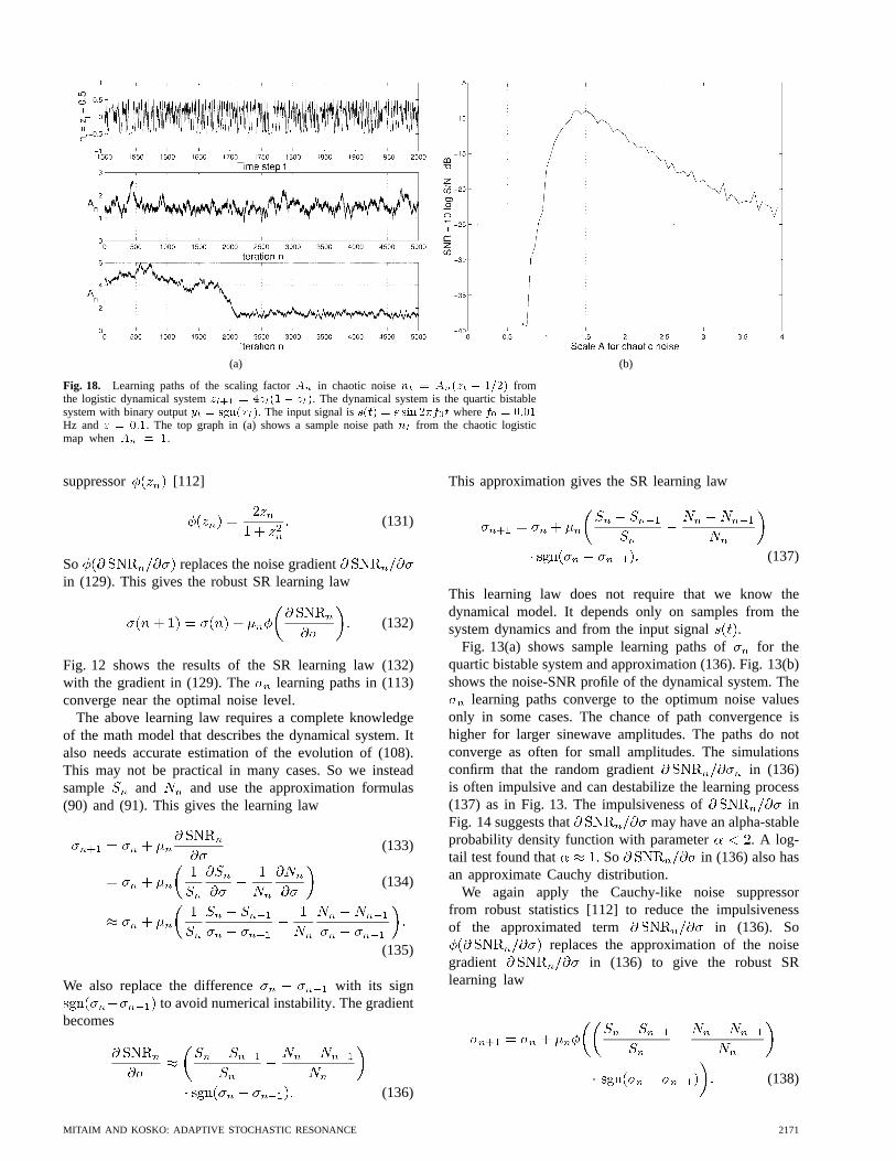
Fig. 18. Learning paths of the scaling factorAn in chaotic noisent = An(zt � 1=2) fromthe logistic dynamical systemzt+1 = 4zt(1� zt). The dynamical system is the quartic bistablesystem with binary outputyt = sgn(xt). The input signal iss(t) = " sin 2�f0t wheref0 = 0:01Hz and " = 0:1. The top graph in (a) shows a sample noise pathnt from the chaotic logisticmap whenAn = 1.

suppressor [112]

(131)

So replaces the noise gradientin (129). This gives the robust SR learning law

(132)

Fig. 12 shows the results of the SR learning law (132)with the gradient in (129). The learning paths in (113)converge near the optimal noise level.

The above learning law requires a complete knowledgeof the math model that describes the dynamical system. Italso needs accurate estimation of the evolution of (108).This may not be practical in many cases. So we insteadsample and and use the approximation formulas(90) and (91). This gives the learning law

(133)

(134)

(135)

We also replace the difference with its signto avoid numerical instability. The gradient

becomes

(136)

This approximation gives the SR learning law

(137)

This learning law does not require that we know thedynamical model. It depends only on samples from thesystem dynamics and from the input signal .

Fig. 13(a) shows sample learning paths of for thequartic bistable system and approximation (136). Fig. 13(b)shows the noise-SNR profile of the dynamical system. The

learning paths converge to the optimum noise valuesonly in some cases. The chance of path convergence ishigher for larger sinewave amplitudes. The paths do notconverge as often for small amplitudes. The simulationsconfirm that the random gradient in (136)is often impulsive and can destabilize the learning process(137) as in Fig. 13. The impulsiveness of inFig. 14 suggests that may have an alpha-stableprobability density function with parameter . A log-tail test found that . So in (136) also hasan approximate Cauchy distribution.

We again apply the Cauchy-like noise suppressorfrom robust statistics [112] to reduce the impulsivenessof the approximated term in (136). So

replaces the approximation of the noisegradient in (136) to give the robust SRlearning law

(138)


(a)

(b)

Fig. 19. SR learning paths of�n for the threshold systemyt = sgn(st + nt � �) wheresgn(x) = 1 if x � 0 and sgn(x) = �1 if x < 0. The input sinewave isst = " sin 2�f0twith additive white Gaussian noise sequencent. The parameters are (a)f0 = 0:001; " = 0:1, and� = 0:5 and (b)f0 = 0:001; " = 0:5, and� = 1.

Fig. 15 shows the results of the SR learning law (138). Thelearning paths converge to the optimum noise level if the

initial value lies close enough to it. Then wanders in asmall Brownian-like motion about the optimum noise level.

Like results hold for other noise densities with finite vari-ance such as Laplace and uniform noise. Fig. 16 showslearning paths for the quartic bistable system (122)–(123)with Laplace noise and uniform noise. We also tested thequartic bistable system with alpha-stable noise. Fig. 17shows the paths of the optimal dispersion for

, and . The learning degrades asfalls and the alpha-stable bell curves have thicker tails.

We also used a chaotic time series as the forcing noisein the quartic bistable dynamical system [118]. The simpleand popular logistic map created the noise sequence

(139)

from the initial value [118]. The positivesequence stays bounded within the unit interval:

. The chaotic noise comes from

(140)

The factor acts as the scaled power or standarddeviation if the term is a zero-mean randomvariable with unit variance. Learning tunes so that thedynamical system shows the SR effect. Fig. 18 shows asample chaotic noise sequence and shows twolearningpaths on their way to stochastic convergence.

B. Other SR Test Cases

The SR learning schemes also work for other SR models.We here show only the results for zero-mean white Gauss-ian noise. We first tested the discrete-time threshold neuronmodel

ifif

(141)


(a)

(b)

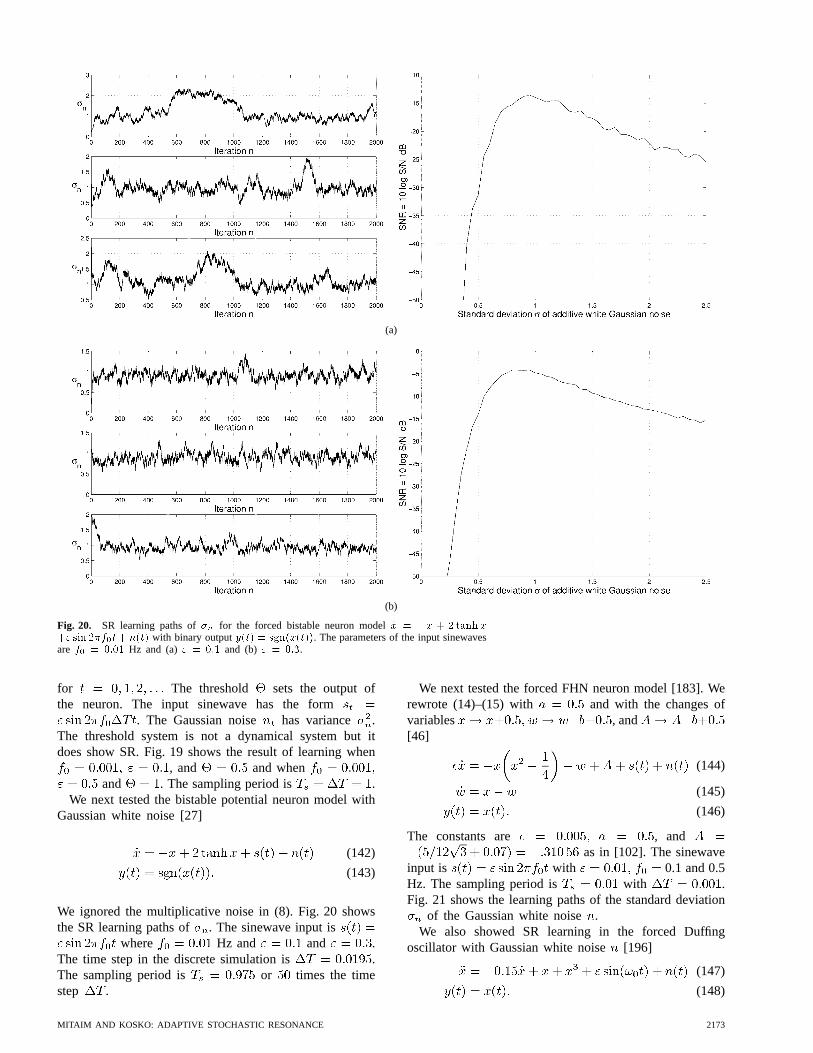
Fig. 20. SR learning paths of�n for the forced bistable neuron model_x = �x + 2tanh x+" sin 2�f0t+ n(t) with binary outputy(t) = sgn(x(t)). The parameters of the input sinewavesare f0 = 0:01 Hz and (a)" = 0:1 and (b) " = 0:3.

for The threshold sets the output ofthe neuron. The input sinewave has the form

. The Gaussian noise has variance .The threshold system is not a dynamical system but itdoes show SR. Fig. 19 shows the result of learning when

, and and whenand . The sampling period is .

We next tested the bistable potential neuron model withGaussian white noise [27]

(142)

(143)

We ignored the multiplicative noise in (8). Fig. 20 showsthe SR learning paths of . The sinewave input is

where Hz and and .The time step in the discrete simulation is .The sampling period is or times the timestep .

We next tested the forced FHN neuron model [183]. Werewrote (14)–(15) with and with the changes ofvariables , and[46]

(144)

(145)

(146)

The constants are , andas in [102]. The sinewave

input is with 0.1 and 0.5Hz. The sampling period is with .Fig. 21 shows the learning paths of the standard deviation

of the Gaussian white noise.We also showed SR learning in the forced Duffing

oscillator with Gaussian white noise [196]

(147)

(148)


(a)

(b)

Fig. 21. SR learning paths of�n for the FHN neuron model� _x = �x(x2 � 1

4) � w + A

+s(t) + n(t) and _w = x � w with output y(t) = x(t). The parameters are� = 0:005 andA = �(5=12

p3 + 0:07) = �:31056. The sinewave input signal iss(t) = " sin 2�f0t where

(a) " = 0:01 and f0 = 0:1 Hz and (b)" = 0:01 and f0 = 0:5 Hz. (a) and (b) show how SRlearning convergence can depend on initial conditions. The distant starting point�0 > 7:5� 10�3

leads to divergence in the third learning sample in (a) but it leads to convergence in the thirdlearning sample in (b).

Fig. 22 shows the learning paths of for input sinewavewith frequency Hz and with amplitudesand . The sampling period is with

.

C. Fuzzy SR Learning: The Quartic Bistable System

We used a fuzzy function approximator tolearn and store the entire surface of optimal noise valuesfor the quartic bistable system with input sinewaves. Thefuzzy system had as its input the 2-D vector of sinewaveamplitude and frequency . We tested the system withthe fixed input initial value . The fuzzy systemitself defined a vector function and used200 rules. The chain rule extended the learning laws inthe previous sections to tune the fuzzy system’s parameters

as in (71)

(149)

(150)

Appendix B derives the partial derivative for thesinc SAM fuzzy system that we used. The Cauchy noisesuppressor gives the learning law as

(151)

Fig. 23 shows how we formed a first set of rules on theproduct space of the two variablesand . It also showshow the learning laws move and shape the width of the


(a)

(b)

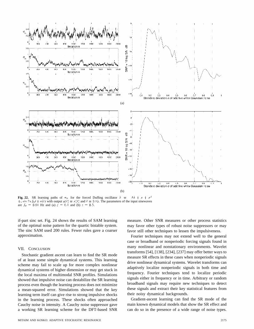
Fig. 22. SR learning paths of�n for the forced Duffing oscillator�x = �� _x + x + x3

+" sin 2�f0t+n(t) with outputy(t) = x(t) and� = 0:15. The parameters of the input sinewavesare f0 = 0:01 Hz and (a)" = 0:1 and (b) " = 0:3.

if-part sinc set. Fig. 24 shows the results of SAM learningof the optimal noise pattern for the quartic bistable system.The sinc SAM used 200 rules. Fewer rules gave a coarserapproximation.

VII. CONCLUSION

Stochastic gradient ascent can learn to find the SR modeof at least some simple dynamical systems. This learningscheme may fail to scale up for more complex nonlineardynamical systems of higher dimension or may get stuck inthe local maxima of multimodal SNR profiles. Simulationsshowed that impulsive noise can destabilize the SR learningprocess even though the learning process does not minimizea mean-squared error. Simulations showed that the keylearning term itself can give rise to strong impulsive shocksin the learning process. These shocks often approachedCauchy noise in intensity. A Cauchy noise suppressor gavea working SR learning scheme for the DFT-based SNR

measure. Other SNR measures or other process statisticsmay favor other types of robust noise suppressors or mayfavor still other techniques to lessen the impulsiveness.

Fourier techniques may not extend well to the generalcase or broadband or nonperiodic forcing signals found inmany nonlinear and nonstationary environments. Wavelettransforms [54], [138], [234], [237] may offer better ways tomeasure SR effects in these cases when nonperiodic signalsdrive nonlinear dynamical systems. Wavelet transforms canadaptively localize nonperiodic signals in both time andfrequency. Fourier techniques tend to localize periodicsignals either in frequency or in time. Arbitrary or randombroadband signals may require new techniques to detectthese signals and extract their key statistical features fromtheir noisy dynamical backgrounds.

Gradient-ascent learning can find the SR mode of themain known dynamical models that show the SR effect andcan do so in the presence of a wide range of noise types.


(a)

(b)

(c) (d)

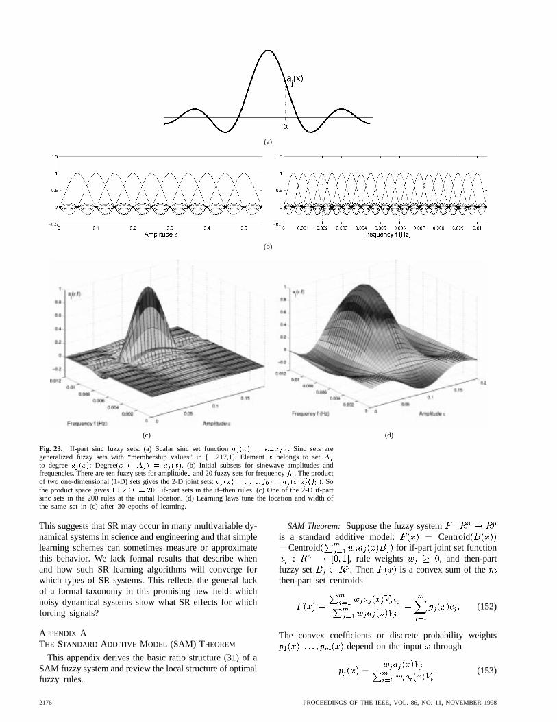
Fig. 23. If-part sinc fuzzy sets. (a) Scalar sinc set functionaj(x) = sin x=x. Sinc sets aregeneralized fuzzy sets with “membership values” in [�.217,1]. Elementx belongs to setAj

to degreeaj(x): Degree(x 2 Aj) = aj(x). (b) Initial subsets for sinewave amplitudes andfrequencies. There are ten fuzzy sets for amplitude" and 20 fuzzy sets for frequencyf0. The productof two one-dimensional (1-D) sets gives the 2-D joint sets:aj(x) = aj("; f0) = a1j (")a

2

j (f0). Sothe product space gives10� 20 = 200 if-part sets in the if–then rules. (c) One of the 2-D if-partsinc sets in the 200 rules at the initial location. (d) Learning laws tune the location and width ofthe same set in (c) after 30 epochs of learning.

This suggests that SR may occur in many multivariable dy-namical systems in science and engineering and that simplelearning schemes can sometimes measure or approximatethis behavior. We lack formal results that describe whenand how such SR learning algorithms will converge forwhich types of SR systems. This reflects the general lackof a formal taxonomy in this promising new field: whichnoisy dynamical systems show what SR effects for whichforcing signals?

APPENDIX ATHE STANDARD ADDITIVE MODEL (SAM) THEOREM

This appendix derives the basic ratio structure (31) of aSAM fuzzy system and review the local structure of optimalfuzzy rules.

SAM Theorem:Suppose the fuzzy systemis a standard additive model: Centroid

Centroid for if-part joint set function, rule weights , and then-part

fuzzy set . Then is a convex sum of thethen-part set centroids

(152)

The convex coefficients or discrete probability weightsdepend on the input through

(153)


(a)

(b)

Fig. 24. Optimal noise levels in terms of the SNR for thequartic bistable system with binary output. (a) The optimum noisepattern when inputs are sinewaves with distinct amplitudes andfrequencies. (b) SAM fuzzy approximation of the optimum noiseafter 30 epochs. The sinc SAM used 200 rules. One epoch used20 iterations that trained on 200 input amplitudes and frequencies.The quartic bistable system has the form_x = x�x

3+s(t)+n(t)with initial condition x(0) = �1. The initialized SAM gave theoutput value 0.2 as its first estimate of the optimal noise level.

is the finite positive volume (or area if ) andis the centroid of then-part set

(154)

(155)

Proof: There is no loss of generality to prove thetheorem for the scalar-output case when

. This simplifies the notation. We need but replace thescalar integrals over with the -multiple or volumeintegrals over in the proof to prove the general case.

The scalar case gives (154) and (155) as

(156)

(157)

Then the theorem follows if we expand thecentroid of and invoke the SAM assumption

Centroid Centroidto rearrange terms

Centroid (158)

(159)

(160)

(161)

(162)

(163)

(164)

Now we give a simplelocal description of optimal lonefuzzy rules [135], [136]. We move a fuzzy rule patch sothat it most reduces an error. We look (locally) at a minimalfuzzy system of just one rule. So the fuzzysystem is constant in that region: . Suppose that

for and define the error

(165)

We want to find the best place. So the first-order conditiongives or

(166)

Then implies that

(167)

at . So the extrema of and coincide in this case.Fig. 7 shows how fuzzy rule patches can “patch the bumps”and so help minimize the error of approximation.

APPENDIX BSAM GRADIENT LEARNING

Supervised gradient ascent can tune all the parametersin the SAM model (31) [134], [136]. A gradient ascentlearning law for a SAM parameter has the form

(168)


where is a learning rate at iteration. We seek tomaximize the performance measure of the dynamicalsystem . Here the SNR defines the performance

.Let denote the th parameter in the set function .

Then the chain rule gives the gradient of the SNR withrespect to , with respect to the then-part set centroid,and with respect to the then-part set volume

and

(169)

We have derived the partial derivativein Section V-B. We next derive the partial

derivatives for the SAM parameters

(170)

(171)

The SAM ratio (31) gives [134]

(172)

and

(173)

Then the learning laws for the centroid and volume havethe final form

(174)

and

(175)

Learning laws for set parameters depend on how wedefine the set functions. The partial derivatives for the scalarsinc set function have theform

forfor

(176)

(177)

So this scalar set function leads to the learning laws

(178)

(179)

Like results hold for the learning laws of product-D set functions. A factored set function

leads to a new form for the performancegradient. The gradient with respect to the parameterofthe th set function has the form

where

(180)

Products of the scalar sinc set functions defined the if-partfuzzy sets in the SAM approximator. Simulationshave shown [174], [175] that sinc set functions tend toperform at least as well as other popular set functions insupervised fuzzy function approximation.

REFERENCES

[1] Y. S. Abu-Mostafa, “Learning from hints in neural networks,”J. Complexity, vol. 6, pp. 192–198, 1990.

[2] , “Hints,” Neural Computation, vol. 7, pp. 639–671, 1995.[3] V. S. Anishchenko, A. B. Neiman, and M. A. Safonova,

“Stochastic resonance in chaotic systems,”J. Statist. Physics,vol. 70, nos. 1/2, pp. 183–196, 1993.

[4] V. S. Anishchenko, M. A. Safonova, and L. O. Chua, “Stochas-tic resonance in Chua’s circuit,”Int. J. Bifurcation and Chaos,vol. 2, no. 2, pp. 397–401, 1992.

[5] , “Stochastic resonance in Chua’s circuit driven by am-plitude or frequency modulated signals,”Int. J. Bifurcation andChaos, vol. 4, no. 2, pp. 441–446, 1994.

[6] A. S. Asdi and A. H. Tewfik, “Detection of weak signals usingadaptive stochastic resonance,” inProc. 1995 IEEE Int. Conf.Acoustics, Speech, and Signal Processing (ICASSP-95), vol. 2,pp. 1332–1335.

[7] P. Babinec, “Stochastic resonance in the Weidlich model ofpublic opinion formation,”Phys.s Lett. A, vol. 225, pp. 179–181,Jan. 1997.

[8] P. Baldi, “Gradient descent learning algorithm overview: Ageneral dynamical systems perspective,”IEEE Trans. NeuralNetworks, vol. 6, pp. 182–195, Jan. 1995.

[9] R. Bartussek, P. Hanggi, and P. Jung, “Stochastic resonancein optical bistable systems,”Phys. Rev. E, vol. 49, no. 5, pp.3930–3939, May 1994.

[10] M. Bartz, “Large-scale dithering enhances ADC dynamicrange,”Microwave & RF, vol. 32, pp. 192–194+, May 1993.

[11] R. Benzi, G. Parisi, A. Sutera, and A. Vulpiani, “Stochasticresonance in climatic change,”Tellus, vol. 34, pp. 10–16, 1982.

[12] , “A theory of stochastic resonance in climatic change,”SIAM J. Appl. Math., vol. 43, no. 3, pp. 565–578, June 1983.

[13] R. Benzi, A. Sutera, and A. Vulpiani, “The mechanism ofstochastic resonance,”J. Physics A: Math. and General, vol.14, pp. L453–L457, 1981.


[14] R. Benzi, A. Sutera, and A. Vulpiani, “Stochastic resonancein the Landau-Ginzberg equation,”J. Physics A: Mathematicaland General, vol. 18, pp. 2239–2245, 1985.

[15] S. M. Bezrukov and I. Vodyanoy, “Stochastic resonance innondynamical systems without response thresholds,”Nature,vol. 385, pp. 319–321, Jan. 1997.

[16] Y. Braiman, J. F. Lindner, and W. L. Ditto, “Taming spatiotem-poral chaos with disorder,”Nature, vol. 378, pp. 465–467, Nov.1995.

[17] H. A. Braun, H. Wissing, K. Schafer, and M. C. Hirsch,“Oscillation and noise determine signal transduction in Sharkmultimodal sensory cells,”Nature, vol. 367, pp. 270–273, Jan.1994.

[18] L. Breiman, Probability. Reading, MA: Addision-Wesley,1968.

[19] J. J. Brey, J. Casado-Pascul, and B. Sanchez, “Resonant behav-ior of a Poisson process driven by a periodic signal,”Phys. Rev.E, vol. 52, no. 6, pp. 6071–6081, Dec. 1995.

[20] J. J. Brey and A. Prados, “Stochastic resonance in a one-dimension Ising model,”Phys.s Lett. A, vol. 216, pp. 240–246,June 1996.

[21] K. S. Brown, “Noises on,”New Scientist, vol. 150, pp. 28–31,June 1996.

[22] P. Bryant, K. Wiesenfeld, and B. McNamara, “The nonlineareffects of noise on parametric amplification: An analysis ofnoise rise in Josephson junctions and other systems,”J. Appl.Physics, vol. 62, no. 7, pp. 2898–2913, Oct. 1987.

[23] A. Bulsara, S. Chillemi, L. Kiss, P. V. E. McClintock, R.Mannella, F. Maresoni, K. Nicolis, and K. Wiesenfeld, Eds.,Il Nuovo Cimento, Special Issue on Fluctuation in Physics andBiology: Stochastic Resonance, Signal Processing, and RelatedPhenomena, Luglio-Agosto, vol. 17 D, nos. 7–8, 1995.

[24] A. R. Bulsara, R. D. Boss, and E. W. Jacobs, “Noise effectsin an electronic model of a single neuron,”Biological Cybern.,vol. 61, pp. 211–222, 1989.

[25] A. R. Bulsara, T. C. Elston, C. R. Doering, S. B. Lowen, and K.Lindenberg, “Cooperative behavior in periodically driven noisyintegrate-fire models of neuronal dynamics,”Phys. Rev. E, vol.53, no. 4, pp. 3958–3969, Apr. 1996.

[26] A. R. Bulsara and L. Gammaitoni, “Tuning in to noise,”Phys.sToday, pp. 39–45, Mar. 1996.

[27] A. R. Bulsara, E. W. Jacobs, T. Zhou, F. Moss, and L.Kiss, “Stochastic resonance in a single neuron model: Theoryand analog simulation,”J. Theoretical Biology, vol. 152, pp.531–555, 1991.

[28] A. R. Bulsara, S. B. Lowen, and C. D. Rees, “Cooperativebehavior in the periodically modulated Wiener process: Noise-induced complexity in a model neuron,”Phys. Rev. E, vol. 49,no. 6, pp. 4989–5000, June 1994.

[29] A. R. Bulsara, A. J. Maren, and G. Schmera, “Single effectiveneuron: Dendritic coupling effects and stochastic resonance,”Biological Cybern., vol. 70, pp. 145–156, 1993.

[30] A. R. Bulsara and G. Schmera, “Stochastic resonance in glob-ally coupled nonlinear oscillators,”Phys. Rev. E, vol. 47, no. 5,pp. 3734–3737, May 1993.

[31] A. R. Bulsara and A. Zador, “Threshold detection of widebandsignals: A noise-induced maximum in the mutual information,”Phys. Rev. E, vol. 54, no. 3, pp. R2185–R2188, Sept. 1996.

[32] G. C. Burdea,Force and Touch Feedback for Virtual Reality.New York: Wiley, 1996.

[33] T. L. Carroll and L. M. Pecora, “Stochastic resonance andcrises,”Phys. Rev. Lett., vol. 70, no. 5, pp. 576–579, Feb. 1993.

[34] J. M. Casado and M. Morillo, “Distribution of escape times ina driven stochastic model,”Phys. Rev. E, vol. 49, no. 2, pp.1136–1139, Feb. 1994.

[35] R. Castro and T. Sauer, “Chaotic stochastic resonance: Noise-enhanced reconstruction of attractors,”Phys. Rev. Lett., vol. 79,no. 6, pp. 1030–1033, Aug. 1997.

[36] F. Chapeau-Blondeau, “Noise-enhanced capacity via stochasticresonance in an asymmetric binary channel,”Phys. Rev. E, vol.55, no. 2, pp. 2016–2019, Feb. 1997.

[37] F. Chapeau-Blondeau and X. Godivier, “Stochastic resonancein nonlinear transmission of Spike signals: An exact model andan application to the neuron,”Int. J. Bifurcation and Chaos, vol.6, no. 11, pp. 2069–2076, 1996.

[38] , “Theory of stochastic resonance in signal transmissionby static nonlinear system,”Phys. Rev. E, vol. 55, no. 2, pp.1478–1495, Feb. 1997.

[39] F. Chapeau-Blondeau, X. Godivier, and N. Chambet, “Stochas-tic resonance in a neuron model that transmits Spike trains,”Phys. Rev. E, vol. 53, no. 1, pp. 1273–1275, Jan. 1996.

[40] A. K. Chattah, C. B. Briozzo, O. Osenda, and M. O. Caceres,“Signal-to-noise ratio in stochastic resonance,”Modern Phys.Lett. B, vol. 10, no. 22, pp. 1085–1094, 1996.

[41] D. R. Chialvo, A. Longtin, and J. Muller-Gerking, “Stochasticresonance in models of neuronal ensembles,”Phys. Rev. E, vol.55, no. 2, pp. 1798–1808, Feb. 1997.

[42] F. Y. Chiou-Tan, K. N. Magee, S. M. Tuel, L. R. Robinson,T. A. Krouskop, M. R. Netson, and F. Moss, “Augmentedsensory nerve action potentials during distant muscle contrac-tion,” Amer. J. Physical Med. Rehab., vol. 76, no. 1, pp. 14–18,Jan./Feb. 1997.

[43] K. L. Chung and R. J. Williams,Introduction to StochasticIntegration, 2nd edition. Boston: Birkhauser, 1990.

[44] J. J. Collins, C. C. Chow, A. C. Capela, and T. T. Imhoff,“Aperiodic stochastic resonance,”Phys. Rev. E, vol. 54, no. 5,pp. 5575–5584, Nov. 1996.

[45] J. J. Collins, C. C. Chow, and T. T. Imhoff, “Aperiodicstochastic resonance in excitable systems,”Phys. Rev. E, vol.52, no. 4, pp. R3321–R3324, Oct. 1995.

[46] , “Stochastic resonance without tuning,”Nature, vol. 376,pp. 236–238, July 1995.

[47] J. J. Collins, T. T. Imhoff, and P. Grigg, “Noise-enhanced in-formation transmission in rat SA1 cutaneous mechanoreceptorsvia aperiodic stochastic resonance,”J. Neurophysiology, vol.76, no. 1, pp. 642–645, July 1996.

[48] , “Noise-enhanced tactile sensation,”Nature, vol. 383, pp.770, Oct. 1996.

[49] P. Cordo, J. T. Inglis, S. Vershueren, J. J. Collins, D. M.Merfeld, S. Rosenblum, S. Buckley, and F. Moss, “Noise inhuman muscle spindles,”Nature, vol. 383, pp. 769–770, Oct.1996.

[50] T. M. Cover and J. A. Thomas,Elements of Information Theory.New York: Wiley, 1991.

[51] J. J. Craig,Introduction to Robotics: Mechanics and Control,2nd edition. Reading, MA: Addison-Wesley, 1989.

[52] A. Crisanti, M. Falcioni, G. Paladin, and A. Vulpiani, “Sto-chastic resonance in deterministic chaotic systems,”J. PhysicsA: Mathematical and General, vol. 27, pp. L597–L603, 1994.

[53] G. Dahlquist andA. Bjorck, Numerical Methods. EnglewoodCliffs, NJ: Prentice-Hall, 1974.

[54] I. Daubechies,Ten Lectures on Wavelets. Philadelphia, PA:SIAM, 1992.

[55] G. Debnath, F. Moss, T. Leiber, H. Risken, and F. Maresoni,“Holes in the two-dimensional probability density of bistablesystems driven by strongly colored noise,”Phys. Rev. A, vol.42, no. 2, pp. 703–710, July 1990.

[56] G. Debnath, T. Zhou, and F. Moss, “Remarks on stochasticresonance,”Phys. Rev. A, vol. 39, no. 8, pp. 4323–4326, Apr.1989.

[57] J. L. Doob,Stochastic Processes. New York: Wiley, 1953.[58] J. K. Douglass, L. Wilkens, E. Pantazelou, and F. Moss, “Noise

enhancement of information transfer in Crayfish mechanorecep-tors by stochastic resonance,”Nature, vol. 365, pp. 337–340,Sept. 1993.

[59] , “Stochastic resonance in Crayfish hydrodynamic recep-tors stimulated with external noise,” inAIP Conf. Proc. 285:Noise in Physical Systems and 1/f Fluctuations, P. H. Haneland A. L. Chung, Eds., 1993, pp. 712–715.

[60] R. Durrett, Stochastic Calculus: A Practical Introduction.Boca Raton, FL: CRC, 1996.

[61] M. I. Dykman, G. P. Golubev, I. K. Kaufman, D. G. Luchinsky,P. V. E. McClintock, and E. A. Zhukov, “Noise-enhancedoptical heterodyning in an all-optical bistable system,”Appl.Phys. Lett., vol. 67, no. 3, pp. 308–310, July 1995.

[62] M. I. Dykman, T. Horita, and J. Ross, “Statistical distributionand stochastic resonance in a periodically driven chemicalsystem,” J. Chemical Physics, vol. 103, no. 3, pp. 966–972,July 1995.

[63] M. I. Dykman, D. G. Luchinsky, R. Mannella, P. V. E.McClintock, S. M. Soskin, and N. D. Stein, “Resonant sub-harmonic absorption and second-harmonic generation by afluctuating nonlinear oscillator,”Phys. Rev. E, vol. 54, no. 3,pp. 2366–2377, Sept. 1996.

[64] M. I. Dykman, D. G. Luchinsky, R. Mannella, P. V. E.McClintock, N. D. Stein, and N. G. Stocks, “Nonconventional


stochastic resonance,”J. Statist. Physics, vol. 70, nos. 1/2, pp.479–499, Jan. 1993.

[65] , “Stochastic resonance: Linear response and giant nonlin-earity,” J. Statist. Physics, vol. 70, nos. 1/2, pp. 463–478, Jan.1993.

[66] , “Supernarrow spectral peaks and high-frequency stochas-tic resonance in systems with coexisting periodic attractors,”Phys. Rev. E, vol. 49, no. 2, pp. 1198–1215, Feb. 1994.

[67] M. I. Dykman, D. G. Luchinsky, P. V. E. McClintock, N. D.Stein, and N. G. Stocks, “Stochastic resonance for periodicallymodulated noise intensity,”Phys. Rev. A, vol. 46, no. 4, pp.R1713–R1716, Aug. 1992.

[68] J.-P. Eckmann and L. E. Thomas, “Remarks on stochasticresonances,”J. Physics A: Mathematical and General, vol. 15,pp. L261–L266, 1982.

[69] S. Fauve and F. Heslot, “Stochastic resonance in a bistablesystem,”Phys.s Lett. A, vol. 97, nos. 1/2, pp. 5–7, Aug. 1983.

[70] W. Feller,An Introduction to Probability Thoery and Its Appli-cations. New York: Wiley, vol. II, 1966.

[71] P. G. Flikkema, “Spread-spectrum techniques for wireless com-munication,”Signal Processing Mag., vol. 14, no. 3, pp. 26–36,1997.

[72] A. Forster, M. Merget, and F. W. Schneider, “Stochastic res-onance in chemistry 2: The peroxidase-oxidase reaction,”J.Physical Chemistry, vol. 100, pp. 4442–4447, 1996.

[73] A. M. Forte and J. X. Mitrovica, “A resonance in the earth’sobliquity and precession over the past 20 Myr driven by mantleconvection,”Nature, vol. 390, pp. 676–680, Dec. 1997.

[74] J. Foss, F. Moss, and J. Milton, “Noise, multistability, anddelayed recurrent loops,”Phys. Rev. E, vol. 55, no. 4, pp.4536–4543, Apr. 1997.

[75] R. F. Fox, “Stochastic resonance in a double well,”Phys. Rev.A, vol. 39, no. 8, pp. 4148–4153, Apr. 1989.

[76] R. F. Fox and Y. N. Lu, “Analytic and numerical studyof stochastic resonance,”Phys. Rev. E, vol. 48, no. 5, pp.3390–3398, Nov. 1993.

[77] W. J. Freeman, H.-J. Chang, B. C. Burke, P. A. Rose, and J.Badler, “Taming chaos: Stabilization of aperiodic attractors bynoise,” IEEE Trans. Circuits Systems I, vol. 44, pp. 989–996,Oct. 1997.

[78] A. Fulinski, “Relaxation, noise-induced transitions, and sto-chastic resonance driven by Non-Markovian dichotomic noise,”Phys. Rev. E, vol. 52, no. 4, pp. 4523–4526, Oct. 1995.

[79] L. Gammaitoni, “Stochastic resonance in multi-threshold sys-tems,” Phys.s Lett. A, vol. 208, pp. 315–322, Dec. 1995.

[80] , “Stochastic resonance,”Rev. Modern Physics, vol. 70,no. 1, pp. 223–287, Jan. 1998.

[81] L. Gammaitoni, F. Maresoni, M. Martinelli, L. Pardi, and S.Santucci, “Phase shifts in bistable EPR systems at stochasticresonance,”Phys.s Lett. A, vol. 158, no. 9, pp. 449–452, Sept.1991.

[82] L. Gammaitoni, F. Maresoni, E. Menichella-Saetta, and S.Santucci, “Stochastic resonance in bistable systems,”Phys. Rev.Lett., vol. 62, no. 4, pp. 349–352, Jan. 1989.

[83] L. Gammaitoni, F. Maresoni, E. Menichella-Saetta, and S.Santucci, “Multiplicative stochastic resonance,”Phys. Rev. E,vol. 49, no. 6, pp. 4878–4881, June 1994.

[84] L. Gammaitoni, M. Martinelli, L. Pardi, and S. Santucci,“Observation of stochastic resonance in bistable electron-paramagnetic-resonance systems,”Phys. Rev. Lett., vol. 67,no. 13, pp. 1799–1802, Sept. 1991.

[85] L. Gammaitoni, E. Menichella-Saetta, S. Santucci, F. Maresoni,and C. Pressilla, “Periodically time-modulated bistable sys-tems: Stochastic resonance,”Phys. Rev. A, vol. 40, no. 4, pp.2114–2119, Aug. 1989.

[86] T. C. Gard,Introduction to Stochastic Differential Equations.New York: Marcel Dekker, 1988.

[87] F. Gassmann, “Noise-induced chaos-order transitions,”Phys.Rev. E, vol. 55, no. 3, pp. 2215–2221, Mar. 1997.

[88] Z. Gingl, L. B. Kiss, and F. Moss, “Non-dynamical stochasticresonance: Theory and experiments with white and arbitrarilycolored noise,”Europhysics Lett., vol. 29, no. 3, pp. 191–196,Jan. 1995.

[89] J. Glanz, “Mastering the nonlinear brain,”Science, vol. 277,pp. 1758–1760, Sept. 1997.

[90] B. J. Gluckman, T. I. Netoff, E. J. Neel, W. L. Ditto, M. L.Spano, and S. J. Schiff, “Stochastic resonance in a neuronalnetwork from mammalian brain,”Phys. Rev. Lett., vol. 77, no.

19, pp. 4098–4101, Nov. 1996.[91] X. Godivier and F. Chapeau-Blondeau, “Noise-assisted signal

transmission in a nonlinear electronic comparator: Experimentand theory,”Signal Processing, vol. 56, pp. 293–303, 1997.

[92] D. C. Gong, G. Hu, X. D. Wen, C. Y. Yang, G. R. Qin, R. Li,and D. F. Ding, “Experimental study of the signal-to-noise ratioof stochastic resonance systems,”Phys. Rev. A, vol. 46, no. 6,pp. 3243–3249, Sept. 1992.

[93] M. Grifoni, “Dynamics of the dissipative two-state system underAC modulation of bias and coupling energy,”Phys. Rev. E, vol.54, no. 4, pp. R3086–R3089, Oct. 1996.

[94] M. Grifoni and P. Hanggi, “Nonlinear quantum stochasticresonance,”Phys. Rev. E, vol. 54, no. 2, pp. 1390–1401, Aug.1996.

[95] M. Grifoni, L. Hartmann, S. Berchtold, and P. Hanggi, “Quan-tum tunneling and stochastic resonance,”Phys. Rev. E, vol. 53,no. 6, pp. 5890–5898, June 1996.

[96] M. Grifoni, M. Sassetti, P. H¨anggi, and U. Weiss, “Cooperativeeffects in the nonlinearly driven Spin-Boson system,”Phys. Rev.E, vol. 52, no. 4, pp. 3596–3607, Oct. 1995.

[97] A. N. Grigorenko and P. I. Nikitin, “Stochastic resonance ina bistable magnetic system,”IEEE Trans. Magn., vol. 31, pp.2491–2493, Sept. 1995.

[98] A. N. Grigorenko, S. I. Nikitin, and G. V. Roschepkin, “Sto-chastic resonance at higher harmonics in monostable systems,”Phys. Rev. E, vol. 56, no. 5, pp. R4907–4910, Nov. 1997.

[99] A. Guderian, G. Dechert, K.-P. Zeyer, and F. W. Schnei-der, “Stochastic resonance in chemistry. 1. The Belousov-Zhabitinsku reaction,”J. Physical Chemistry, vol. 100, pp.4437–4441, 1996.

[100] S. Haykin, Neural Networks: A Comprehensive Foundation.Mew York: McMillan, 1994.

[101] R. Hecht-Nielsen,Neurocomputing. Reading, MA: Addison-Wesley, 1990.

[102] C. Heneghan, C. C. Chow, J. J. Collins, T. T. Imhoff, S. B.Lowen, and M. C. Teich, “Information measures quantifyingaperiodic stochastic resonance,”Phys. Rev. E, vol. 54, no. 3,pp. R2228–R2231, 1996.

[103] A. Hibbs, E. W. Jacobs, J. Bekkedahl, A. R. Bulsara, and F.Moss, “Signal enhancement in a r.f. SQUID using stochasticresonance,”Il Nuovo Cimento, Luglio-Agosto, vol. 17 D, nos.7–8, pp. 811–817, 1995.

[104] A. D. Hibbs, A. L. Singsaas, E. W. Jacobs, A. R. Bulsara, J. J.Bekkedahl, and F. Moss, “Stochastic resonance in a supercon-ducting loop with Josephson junction,”J. Appl. Physics, vol.77, no. 6, pp. 2582–2590, Mar. 1995.

[105] W. Hohmann, J. M¨uller, and F. W. Schneider, “Stochasticresonance in chemistry. 3. The minimal-bromate reaction,”J.Physical Chemistry, vol. 100, pp. 5388–4492, 1996.

[106] R. Hollands,The Virtual Reality Home Brewer’s Handbook.New York: Wiley, 1996.

[107] G. Hu, T. Ditzinger, C. Z. Ning, and H. Haken, “Stochasticresonance without external periodic force,”Phys. Rev. Lett., vol.71, no. 6, pp. 807–810, Aug. 1993.

[108] G. Hu, D. C. Gong, X. D. Wen, C. Y. Yang, G. R. Qing, andR. Li, “Stochastic resonance in a nonlinear system driven by anaperiodic force,”Phys. Rev. A, vol. 46, no. 6, pp. 3250–3254,Sept. 1992.

[109] G. Hu, H. Haken, and C. Z. Ning, “A study of stochasticresonance without adiabatic approximation,”Phys. Lett. A, vol.172, nos. 1/2, pp. 21–28, Dec. 1992.

[110] G. Hu, H. Haken, and F. Xie, “Stochastic resonance withsensitive frequency dependence in globally coupled continuoussystems,”Phys. Rev. Lett., vol. 77, no. 10, pp. 1925–1928, Sept.1996.

[111] G. Hu, G. Nicolis, and N. Nicolis, “Periodically forced Fokker-Planck equation and stochastic resonance,”Phys. Rev. A, vol.42, no. 4, pp. 2030–2041, Aug. 1990.

[112] P. J. Huber,Robust Statistics. New York: Wiley, 1981.[113] B. A. Huberman and R. M. Lukose, “Social dilemmas and

internet congestion,”Science, vol. 277, pp. 535–537, July 1997.[114] M. E. Inchiosa and A. R. Bulsara, “Coupling enhances sto-

chastic resonance in nonlinear dynamic elements driven by asinusoidal plus noise,”Phys.s Lett. A, vol. 200, pp. 283–288,Apr. 1995.

[115] , “Nonlinear dynamic elements with noisy sinusoidal forc-ing: Enhancing response via nonlinear coupling,”Phys. Rev. E,vol. 52, no. 1, pp. 327–339, July 1995.


[116] , “Signal detection statistics of stochastic resonators,”Phys. Rev. E, vol. 53, no. 3, pp. R2021–R2024, Mar. 1996.

[117] M. E. Inchiosa, A. R. Bulsara, and L. Gammaitoni, “Higher-order resonant behavior in asymmetric nonlinear stochasticsystems,”Phys. Rev. E, vol. 55, no. 4, pp. 4049–4056, Apr.1997.

[118] E. Ippen, J. Lindner, and W. L. Ditto, “Chaotic resonance: Asimulation,” J. Statist. Physics, vol. 70, nos. 1/2, pp. 437–450,Jan. 1993.

[119] J.-S. R. Jang, C.-T. Sun, and E. Mizutani,Neurofuzzy andSoft Computing: A Computational Approach to Learning andMachine Intelligence. Englewoods Cliffs, NJ: Prentice-Hall,1996.

[120] B. M. Jost and B. E. A. Saleh, “Signal-to-noise ratio improve-ment by stochastic resonance in a unidirectional photorefractivering resonator,”Optics Lett., vol. 21, no. 4, pp. 287–289, Feb.1996.

[121] P. Jung, “Thermal activation in bistable systems under externalperiodic forces,”Zeitschrift fur Physik B, vol. 76, pp. 521–535,1989.

[122] P. Jung, “Threshold devices: Fractal noise and neural talk,”Phys. Review E, vol. 50, no. 4, pp. 2513–2522, Oct. 1994.

[123] , “Stochastic resonance and optimal design of thresholddetectors,”Phys.s Lett. A, vol. 207, pp. 93–104, Oct. 1995.

[124] P. Jung, U. Behn, E. Pantazelou, and F. Moss, “Collectiveresponse in globally coupled bistable systems,”Phys. Rev. A,vol. 46, no. 4, pp. R1709–R1712, Aug. 1992.

[125] P. Jung and P. Hanggi, “Resonantly driven Brownian motion:Basic concepts and exact results,”Phys. Rev. A, vol. 41, no. 6,pp. 2977–2988, Mar. 1990.

[126] P. Jung and P. Hanggi, “Amplification of small signals viastochastic resonance,”Phys. Rev. A, vol. 44, no. 12, pp.8032–8042, Dec. 1991.

[127] P. Jung and P. Talkner, “Suppression of higher harmonics atnoise induced resonances,”Phys. Rev. E, vol. 51, no. 3, pp.2640–2643, Mar. 1995.

[128] P. Jung and K. Wiesenfeld, “Too quiet to hear a whisper,”Nature, vol. 385, p. 291, Jan. 1997.

[129] S. Kadar, J. Wang, and K. Showalter, “Noise-supported trav-elling waves in sub-excitable media,”Nature, vol. 391, pp.770–772, Feb. 1998.

[130] H. M. Kim and B. Kosko, “Neural fuzzy motion estimationand compensation,”IEEE Trans. Signal Processing, vol. 45,pp. 2515–2532, Oct. 1997.

[131] L. B. Kiss, “Possible breakthrough: Significant improvementof signal to noise ratio by stochastic resonance,” inAIP Conf.Proc. 375: Chaotic, Fractal, and Nonlinear Signal Processing,1995, R. A. Katz, Ed., pp. 382–396.

[132] B. Kosko, Neural Networks and Fuzzy Systems: A Dynami-cal Systems Approach to Machine Intelligence. EnglewoodsCliffs, NJ: Prentice-Hall, 1991.

[133] , “Fuzzy systems as universal approximators,”IEEE Trans.Comput., vol. 43, pp. 1329–1333, Nov. 1994.

[134] , “Combining fuzzy systems,” inProc. IEEE Int. C. FuzzySystems (IEEE FUZZ-95), pp. 1855–1863.

[135] , “Optimal fuzzy rules cover extrema,”Int. J. Intell. Syst.,vol. 10, no. 2, pp. 249–255, Feb. 1995.

[136] , Fuzzy Engineering. Englewood Cliffs, NJ: Prentice-Hall, 1996.

[137] I. Kotlasi, “On random variables whose quotient followsthe Cauchy law,”Colloquium Mathematicum, vol. VII, pp.277–284, 1960.

[138] J. Kovacevic and I. Daubechies, Eds.,Proc. IEEE, vol. 84, no.4, 1996.

[139] H. A. Kramers, “Brownian motion in a field of force and thediffusion model of chemical reactions,”Phys., vol. VII, no. 4,pp. 284–304, Apr. 1940.

[140] D. M. Kreps,A Course in Microeconomic Theory. Princeton,NJ: Princeton Univ. Press, 1990.

[141] R. G. Laha, “On a class of distribution functions where thequotients follows the Cauchy law,”Trans. Amer. Math. Soc.,vol. 93, pp. 205–215, Nov. 1959.

[142] W. C. Y. Lee,Mobile Cellular Telecommunications: Analog andDigital Systems. New York: McGraw-Hill, 1995.

[143] W. E. Leland, M. S. Taqqu, W. Willinger, and D. V. Wilson,“On the self-similar nature of ethernet traffic,” inComput.Commun. Rev.: Proc. SIGCOMM-93, vol. 23, pp. 183–193.

[144] D. S. Leonard, “Stochastic resonance in a random walk,”Phys.Rev. A, vol. 46, no. 10, pp. 6742–6744, Nov. 1992.

[145] D. S. Leonard and L. E. Reichl, “Stochastic resonance in achemical reaction,”Phys. Rev. E, vol. 49, no. 2, pp. 1734–1737,Feb. 1994.

[146] J. E. Levin and J. P. Miller, “Broadband neural encodingin the cricket cercal sensory system enhanced by stochasticresonance,”Nature, vol. 380, pp. 165–168, Mar. 1996.

[147] P. H. Lewis and C. Yang,Basic Control Systems Engineering.Englewood Cliffs, NJ: Prentice-Hall, 1997.

[148] R. Li, G. Hu, C. Y. Yang, X. D. Wen, G. R. Qing, and H. J.Zhu, “Stochastic resonance in bistable systems subject to signaland quasimonochromatic noise,”Phys. Rev. E, vol. 51, no. 5,pp. 3964–3967, May 1995.

[149] J. F. Lindner, B. K. Meadows, W. L. Ditto, M. E. Inchiosa, andA. R. Bulsara, “Scaling laws for spatiotemporal synchronizationand array enhanced stochastic resonance,”Phys. Rev. E, vol. 53,no. 3, pp. 2081–2086, Mar. 1996.

[150] S. P. Lipshitz, R. A. Wannamaker, and J. Vanderkooy, “Quan-tization and dither: A theoretical survey,”J. Audio Eng. Soc.,vol. 40, no. 5, pp. 355–374, May 1992.

[151] M. Locher, G. A. Johnson, and E. R. Hunt, “Spatiotemporalstochastic resonance in a system of coupled diode resonators,”Phys. Rev. Lett., vol. 77, no. 23, pp. 4698–4701, Dec. 1996.

[152] K. Loerincz, Z. Gingl, and L. B. Kiss, “A stochastic resonatoris able to greatly improve signal-to-noise ratio,”Phys. Lett. A,vol. 224, pp. 63–67, Dec. 1996.

[153] R. Lofstedt and S. N. Coppersmith, “Quantum stochastic reso-nance,”Phys. Rev. Lett., vol. 72, no. 13, pp. 1947–1950, Mar.1994.

[154] A. Longtin, “Stochastic resonance in neuron models,”J. Statist.Physics, vol. 70, nos. 1/2, pp. 309–327, Jan. 1993.

[155] , “Synchronization of the stochastic FitzHugh–Nagumoequations to periodic forcing,”Il Nuovo Cimento, Luglio-Agosto, vol. 17 D, nos. 7–8, pp. 835–846, 1995.

[156] , “Autonomous stochastic resonance in bursting neurons,”Phys. Rev. E, vol. 55, no. 1, pp. 868–876, Jan. 1997.

[157] A. Longtin, A. R. Bulsara, and F. Moss, “Time-interval se-quences in bistable systems and the noise-induced transmissionof information by sensory neurons,”Phys. Rev. Lett., vol. 67,no. 5, pp. 656–659, July 1991.

[158] A. Longtin, A. R. Bulsara, D. Pierson, and F. Moss, “Bistabilityand the dynamics of periodically forced sensory neurons,”Biological Cybern., vol. 70, pp. 569–578, 1994.

[159] A. Longtin and K. Hinzer, “Encoding with bursting, sub-threshold oscillations, and noise in mammalian cold receptors,”Neural Computation, vol. 8, pp. 215–255, 1996.

[160] V. Loreto, G. Paladin, and A. Vulpiani, “Concept of complexityin random dynamical systems,”Phys. Rev. E, vol. 53, no. 3, pp.2087–2098, Mar. 1996.

[161] J. Maddox, “Toward the brain-computer’s code?,”Nature, vol.352, p. 469, Aug. 1991.

[162] , “Bringing more order out of noisiness,”Nature, vol. 369,p. 271, May 1994.

[163] M. C. Mahato and S. R. Shenoy, “Hysteresis loss and stochasticresonance: A numerical study of a double-well potential,”Phys.Rev. E, vol. 50, no. 4, pp. 2503–2512, Oct. 1994.

[164] D. E. Makarov and N. Makri, “Stochastic resonance and non-linear response in double-quantum-well structures,”Phys. Rev.B, vol. 52, no. 4, pp. R2257–R2260, July 1995.

[165] R. N. Mantegna and B. Spagnolo, “Stochastic resonance in atunnel diode,”Phys. Rev. E, vol. 49, no. 3, pp. R1792–R1795,Mar. 1994.

[166] R. N. Mantegna and B. Spagnolo, “Stochastic resonance in atunnel diode in the presence of white or colored noise,”Il NuovoCimento, Luglio-Agosto, vol. 17 D, nos. 7–8, pp. 873–881,1995.

[167] F. Maresoni, L. Gammaitoni, and A. R. Bulsara, “Spatiotem-poral stochastic resonance in a4 model of Kink-Antikinknucleation,”Phys. Rev. Lett., vol. 76, no. 15, pp. 2609–2612,Apr. 1996.

[168] K. Matsumoto and I. Tsuda, “Noise-induced order,”J. Statist.Physics, vol. 31, no. 1, pp. 87–106, 1983.

[169] B. McNamara and K. Wiesenfeld, “Theory of stochastic res-onance,”Phys. Rev. A, vol. 39, no. 9, pp. 4854–4869, May1989.

[170] B. McNamara, K. Wiesenfeld, and R. Roy, “Observation ofstochastic resonance in a ring laser,”Phys. Rev. Lett., vol. 60,no. 25, pp. 2626–2629, June 1988.

[171] V. I. Melnikov, “Schmitt trigger: A solvable model of stochastic


resonance,”Phys. Rev. E, vol. 48, no. 4, pp. 2481–2489, Oct.1993.

[172] J. P. Miller, G. A. Jacobs, and F. E. Theunissen, “Repre-sentation of sensory information in the cricket cercal sensorysystem. I. Response properties of the primary interneurons,”J.Neurophysiology, vol. 66, no. 5, pp. 1680–1689, Nov. 1991.

[173] , “Representation of sensory information in the cricketcercal sensory system. II. Information theoretic calculationof system accuracy and optimal tuning-curve widths of fourprimary interneurons,”J. Neurophysiology, vol. 66, no. 5, pp.1690–1703, Nov. 1991.

[174] S. Mitaim and B. Kosko, “What is the best shape for a fuzzyset in function approximation?,” inProc. 5th IEEE Int. Conf.Fuzzy Systems (FUZZ-96), vol. 2, pp. 1237–1243.

[175] , “Adaptive joint fuzzy sets for function approximation,”in Proc. 1997 IEEE Int. Conf. Neural Networks (ICNN-97), vol.1, pp. 537–542.

[176] J. Moody and C. Darken, “Fast learning in networks oflocally-tuned processing unit,”Neural Computation, no. 2,pp. 281–294, 1989.

[177] M. Morillo, J. Gomez-Ordo nez, and J. M. Casado, “Stochasticresonance in a mean-field model of cooperative behavior,”Phys.Rev. E, vol. 52, no. 1, pp. 316–320, July 1995.

[178] R. P. Morse and E. F. Evans, “Enhancement of vowel codingfor cochlear implants by addition of noise,”Nature Medicine,vol. 2, no. 8, pp. 928–932, Aug. 1996.

[179] F. Moss, “Stochastic resonance: From the ice ages to the mon-key’s ear,” in Contemporary Problems in Statistical Physics,G. H. Weiss, Ed. Philadelphia, PA: SIAM, 1994, ch. 5, pp.205–253

[180] , “Noisy waves,”Nature, vol. 391, pp. 743–744, Feb. 1998.[181] F. Moss, A. Bulsara, and M. Shlesinger, Eds.,J. Statist. Physics,

Special Issue on Stochastic Resonance in Physics and Biology(Proc. NATO Advanced Research Workshop), Jan. 1993, vol.70, nos. 1/2.

[182] F. Moss, F. Chiou-Tan, and R. Klinke, “Will there be noise intheir ears?,”Nature Medicine, vol. 2, no. 8, pp. 860–862, Aug.1996.

[183] F. Moss, J. K. Douglass, L. Wilkens, D. Pierson, andE. Pantazelou, “Stochastic resonance in an electronicFitzHugh–Nagumo model,” inAnn. New York Academy ofSciences Volume 706: Stochastic Processes in Astrophysics, J.R. Buchler and H. E. Kandrup, Eds., pp. 26–41, 1993.

[184] F. Moss and P. V. E. McClintock, Eds.,Noise in NonlinearDynamical Systems, vol. I–III. Cambridge, UK: CambridgeUniversity Press, 1989.

[185] F. Moss, D. Pierson, and D. O’Gorman, “Stochastic resonance:Tutorial and update,”Int. J. Bifurcation and Chaos, vol. 4, no.6, pp. 1383–1397, 1994.

[186] F. Moss and K. Wiesenfeld, “The benefits of background noise,”Scientific Amer., vol. 273, no. 2, pp. 66–69, Aug. 1995.

[187] D. C. Munson, “A note on lena,”IEEE Trans. Image Processing,vol. 5, p. 3, Jan. 1996.

[188] Z. Neda, “Stochastic resonance in Ising systems,”Phys. Rev. E,vol. 51, no. 6, pp. 5315–5317, June 1995.

[189] A. Neiman and L. Schimansky-Geier, “Stochastic resonancein two coupled bistable systems,”Phys. Lett. A, vol. 197, pp.379–386, Feb. 1995.

[190] A. Neiman, L. Schimansky-Geier, and F. Moss, “Linear re-sponse theory applied to stochastic resonance in models ofensembles of oscillators,”Phys. Rev. E, vol. 56, no. 1, pp.R9–R12, July 1997.

[191] A. Neiman, B. Shulgin, V. Anishchenko, W. Ebeling, L.Schimansky-Geier, and J. Freund, “Dynamic entropies appliedto stochastic resonance,”Phys. Rev. Lett., vol. 76, no. 23, pp.4299–4302, June 1996.

[192] A. Neiman and W. Sung, “Memory effects on stochastic reso-nance,”Phys.s Lett. A, vol. 223, pp. 341–347, Dec. 1996.

[193] C. Nicolis, “Stochastic aspects of climatic transi-tions—Response to a periodic forcing,”Tellus, vol. 34,pp. 1–9, 1982.

[194] , “Long-term climatic transitions and stochastic reso-nance,” J. Statist. Physics, vol. 70, nos. 1/2, pp. 4–14, Jan.1993.

[195] C. Nicolis and G. Nicolis, “Stochastic aspects of climate tran-sitions—Additive fluctuations,”Tellus, vol. 33, pp. 225–234,1981.

[196] G. Nicolis, C. Nicolis, and D. McKernan, “Stochastic resonance

in chaotic dynamics,”J. Statist. Physics, vol. 70, nos. 1/2, pp.125–139, Jan. 1993.

[197] P. Niyogi and F. Girosi, “On the relationship between gener-alization errors hypothesis complexity and sample complexityfor radial basis functions,”Neural Computation, vol. 8, pp.819–842, 1996.

[198] K. Ogata,Modern Control Engineering, 3rd ed. EnglewoodCliffs, NJ: Prentice-Hall, 1997.

[199] A. V. Oppenheim and R. W. Schafer,Discrete-Time SignalProcessing. Englewood Cliffs, NJ: Prentice Hall, 1989.

[200] P. J. Pacini and B. Kosko, “Adaptive fuzzy frequency hopper,”IEEE Trans. Commun., vol. 43, no. 6, pp. 2111–2117, June1995.

[201] A. Restrepo (Palacios), L. F. Zuluaga, and L. E. Pino, “Optimalnoise levels for stochastic resonance,” inProc. 1997 IEEE Int.Conf. Acoustics, Speech, and Signal Processing (ICASSP-97),vol. III, pp. 2365–2368.

[202] E. Pantazelou, C. Dames, F. Moss, J. Douglass, and L. Wilkens,“Temperature dependence and the role of internal noise in signaltransduction efficiency of Crayfish mechanoreceptors,”Int. J.Bifurcation and Chaos, vol. 5, no. 1, pp. 101–108, 1995.

[203] H. C. Papadopoulos and G. W. Wornell, “A class of stochasticresonance systems for signal processing applications,” inProc.1996 IEEE Int. Conf. Acoustics, Speech, and Signal Processing(ICASSP-96), pp. 1617–1620.

[204] A. Papoulis,Probability and Statistics. Englewood Cliffs, NJ:Prentice-Hall, 1990.

[205] T. P. Pareek, M. C. Mahato, and A. M. Jayannavar, “Stochasticresonance and nonlinear response in a dissipative quantum two-state system,”Phys. Rev. B, vol. 55, no. 15, pp. 9318–9321,Apr. 1997.

[206] B. R. Parnas, “Noise and neuronal populations conspire toencode simple waveforms reliably,”IEEE Trans. BioMed. Eng.,vol. 43, pp. 313–318, Mar. 1996.

[207] X. Pei, K. Bachmann, and F. Moss, “The detection threshold,noise and stochastic resonance in the Fitzhugh-Nagumo neuronmodel,” Phys. Lett. A, vol. 206, pp. 61–65, Oct. 1995.

[208] X. Pei, L. Wilkens, and F. Moss, “Light enhances hydrodynamicsignaling in the multimodal caudal photoreceptor interneu-rons of the Crayfish,”J. Neurophysiology, vol. 76, no. 5, pp.3002–3011, Nov. 1996.

[209] X. Pei, L. Wilkens, and F. Moss, “Noise-mediated Spike timingprecision from aperiodic stimuli in an array of Hodgkin-Huxley-type neurons,”Phys. Rev. Lett., vol. 77, no. 22, pp. 4679–4682,Nov. 1996.

[210] D. Pierson, J. K. Douglass, E. Pantazelou, and F. Moss, “Usingan electronic FitzHugh-Nagumo simulator to mimic noisy elec-trophysiological data from stimulated Crayfish mechanoreceptorcells,” in AIP Conf. Proc. 285: Noise in Physical Systems and1/f Fluctuations, P. H. Hanel and A. L. Chung, Eds., 1993, pp.731–734.

[211] H. E. Plesser and S. Tanaka, “Stochastic resonance in a modelneuron with reset,”Phys.s Lett. A, vol. 225, pp. 228–234, Feb.1997.

[212] W.-J. Rappel and A. Karma, “Noise-induced coherence in neu-ral networks,”Phys. Rev. Lett., vol. 77, no. 15, pp. 3256–3259,Oct. 1996.

[213] W.-J. Rappel and S. H. Strogatz, “Stochastic resonance in anautonomous system with a nonuniform limit cycle,”Phys. Rev.E, vol. 50, no. 4, pp. 3249–3250, Oct. 1994.

[214] D. O. Reale, A. K. Pattanayak, and W. C. Schieve, “Semiquantalcorrections to stochastic resonance,”Phys. Rev. E, vol. 51, no.4, pp. 2925–2932, Apr. 1995.

[215] M. Riani and E. Simonotto, “Stochastic resonance in the per-ceptual interpretation of ambiguous figures: A neural networkmodel,” Phys. Rev. Lett., vol. 72, no. 19, pp. 3120–3123, May1994.

[216] M. Riani and E. Simonotto, “Periodic perturbation of ambiguousfigure: A neural network model and a nonsimulated experi-ment,” Il Nuovo Cimento, Luglio-Agosto, vol. 17 D, nos. 7–8,pp. 903–913, 1995.

[217] T. F. Ricci and C. Scherer, “Linear response and stochasticresonance of superparamagnets,”J. Statist. Physics, vol. 86, no.3/4, pp. 803–819, Feb. 1997.

[218] H. Risken,The Fokker-Planck Equation: Methods of Solutionand Application. New York: Springer-Verlag, 1984.

[219] H. Robbins and S. Monro, “A stochastic approximationmethod,”Ann. Math. Statist., vol. 22, pp. 400–407, 1951.


[220] R. Rouse, S. Han, and J. E. Lukens, “Flux amplification us-ing stochastic superconducting quantum interference devices,”Appl. Physics Letters, vol. 66, no. 1, pp. 108–110, Jan. 1995.

[221] S. Russell and P. Norvig,Artificial Intelligence: A ModernApproach. Englewood Cliffs, NJ: Prentice-Hall, 1995.

[222] D. W. E. Schobben, R. A. Beuker, and W. Oomen, “Dither anddata compression,”IEEE Trans. Signal Processing, vol. 45, pp.2097–2101, Aug. 1997.

[223] M. Shao and C. L. Nikias, “Signal processing with fractionallower order moments: Stable processes and their applications,”Proc. IEEE, vol. 81, pp. 984–1010, July 1993.

[224] , Signal Processing with Alpha-Stable Distributions andApplications. New York: Wiley, 1995.

[225] V. A. Shneidman, P. Jung, and P. H¨anggi, “Power spectrum ofa driven bistable system,”Europhysics Lett., vol. 26, no. 8, pp.571–576, June 1994.

[226] S. W. Sides, R. A. Ramos, P. A. Rikvold, and M. A. Novotny,“Kinetic Ising system in an oscillating external field: Stochasticresonance and residence-time distributions,”J. Appl. Physics,vol. 81, no. 8, pp. 5597–5599, Apr. 1997.

[227] M. K. Simon, J. K. Omura, R. A. Scholtz, and B. K. Levitt,Spread Spectrum Communications Handbook. New York:McGraw-Hill, 1994.

[228] E. Simonotto, M. Riani, C. Seife, M. Roberts, J. Twitty, and F.Moss, “Visual perception of stochastic resonance,”Phys. Rev.Lett., vol. 78, no. 6, pp. 1186–1189, Feb. 1997.

[229] C. Smith and C. Gervelis,Cellular System Design and Opti-mization. New York: McGraw-Hill, 1996.

[230] M. L. Spano, M. Wun-Fogle, and W. L. Ditto, “Experimentalobservation of stochastic resonance in a magnetoelastic ribbon,”Phys. Rev. A, vol. 46, no. 8, pp. 5253–5256, Oct. 1992.

[231] M. Stemmler, “A single Spike suffices: The simplest form ofstochastic resonance in model neurons,”Network: Computationin Neural Systems, vol. 7, pp. 687–716, 1996.

[232] N. G. Stocks, N. D. Stein, and P. V. E. McClintock, “Stochasticresonance in monostable systems,”J. Physics A: Math. General,vol. 26, pp. L385–L390, 1993.

[233] N. G. Stocks, N. D. Stein, S. M. Soskin, and P. V. E.McClintock, “Zero-dispersion stochastic resonance,”J. PhysicsA: Math. General, vol. 25, pp. L1119–L1125, 1992.

[234] G. Strang and T. Q. Nguyen,Wavelets and Filter Banks.Cambridge, UK: Wellesley-Cambridge Press, 1996.

[235] M. Thorwart and P. Jung, “Dynamical hysteresis in bistablequantum systems,”Phys. Rev. Lett., vol. 78, no. 13, pp.2503–2506, Mar. 1997.

[236] G. Vemuri and R. Roy, “Stochastic resonance in a bistable ringlaser,”Phys. Rev. A, vol. 39, no. 9, pp. 4668–4674, May 1989.

[237] M. Vetterli and J. Kovacevic, Wavelets and Subband Coding.Englewood Cliffs, NJ: Prentice Hall, 1995.

[238] J. M. G. Vilar and J. M. Rubı, “Divergent signal-to-noise ratioand stochastic resonance in monostable systems,”Phys. Rev.Lett., vol. 77, no. 14, pp. 2863–2866, Sept. 1996.

[239] , “Spatiotemporal stochastic resonance in the Swift-Hohenberg equation,”Phys. Rev. Lett., vol. 78, no. 15, pp.2886–2889, Apr. 1997.

[240] , “Stochastic multiresonance,”Phys. Rev. Lett., vol. 78, no.15, pp. 2882–2885, Apr. 1997.

[241] S. T. Vohra and F. Bucholtz, “Observation of stochastic reso-nance near a subcritical bifurcation,”J. Statist. Physics, vol. 70,nos. 1/2, pp. 413–421, Jan. 1993.

[242] S. T. Vohra and L. Fabiny, “Induced stochastic resonance neara subcritical bifurcation,”Phys. Rev. E, vol. 50, no. 4, pp.R2391–2394, Oct. 1994.

[243] K. Wiesenfeld and F. Moss, “Stochastic resonance and thebenefits of noise: From ice ages to Crayfish and SQUID’s,”Nature, vol. 373, pp. 33–36, Jan. 1995.

[244] K. Wiesenfeld, D. Pierson, E. Pantazelou, C. Dames, and F.Moss, “Stochastic resonance on a circle,”Phys. Rev. Lett., vol.72, pp. 2125–2129, Apr. 1994.

[245] I. J. Winograd, T. B. Coplen, J. M. Landwehr, A. C. Riggs,K. R. Ludwig, B. J. Szabo, P. T. Kolesar, and K. M. Revesz,“Continuous 500,000-year climate record from vein calcite indevils hole, nevada,”Science, vol. 258, pp. 255–260, Oct. 1992.

[246] H. S. Wio, “Stochastic resonance in a spatially extended sys-tem,” Phys. Rev. E, vol. 54, no. 4, pp. R3075–3078, Oct.1996.

[247] A. Witt, A. Neiman, and J. Kurths, “Characterizing the dynam-ics of stochastic bistable systems by measures of complexity,”Phys. Rev. E, vol. 55, no. 5, pp. 5050–5059, May 1997.

[248] W. Yang, M. Ding, and G. Hu, “Trajectory (phase) selection inmultistable systems: Stochastic resonance, signal bias, and theeffect of signal phase,”Phys. Rev. Lett., vol. 74, no. 20, pp.3955–3958, May 1995.

[249] T. Zhou and F. Moss, “Analog simulations of stochastic res-onance,” Phys. Rev. A, vol. 41, no. 8, pp. 4255–4264, Apr.1990.

[250] T. Zhou, F. Moss, and P. Jung, “Escape-time distributions of aperiodically modulated bistable system with noise,”Phys. Rev.A, vol. 42, no. 6, pp. 3161–3169, Sept. 1990.

[251] S. Zozor and P.-O. Amblard, “Stochastic resonance in a discretetime nonlinear SETAR(1,2,0,0) model,” inProc. 1997 IEEEWorkshop Higher-Order-Statistics, July 1997.

[252] U. Zurcher and C. R. Doering, “Thermally activated escapeover fluctuating barriers,”Phys. Rev. E, vol. 47, no. 6, pp.3862–3869, June 1993.

Sanya Mitaim was born in Bangkok, Thailand,in 1970. He received the B.Eng. degree in con-trol engineering from King Mongkut’s Instituteof Technology, Ladkrabang, Thailand in 1990and the M.S. degree in electrical engineeringfrom the University of Southern California, LosAngeles, in 1992. He is currently a Ph.D. can-didate in electrical engineering at the Universityof Southern California.

He was a Lecturer at Thammasat University,Thailand, from 1990 to 1991. His research in-

terests include neural and fuzzy techniques in nonlinear signal processing,software agents, and noise processing.

Bart Kosko (Member, IEEE), for a photograph and biography, see thisissue, p. 2120.


adaptive stochastic resonancesipi.usc.edu/~kosko/adaptivesr.pdf · adaptive stochastic resonance...

Documents