Adaptive Sampling for Rapidly Matching Histograms

Stephen Macke†, Yiming Zhang‡, Silu Huang†, Aditya Parameswaran†University of Illinois-Urbana Champaign

†smacke,shuang86,adityagp@illinois.edu | ‡ym_zhang@sjtu.edu.cn

ABSTRACTIn exploratory data analysis, analysts often have a need to identifyhistograms that possess a specific distribution, among a large classof candidate histograms, e.g., find countries whose income distri-bution is most similar to that of Greece. This distribution couldbe a new one that the user is curious about, or a known distri-bution from an existing histogram visualization. At present, thisprocess of identification is brute-force, requiring the manual gener-ation and evaluation of a large number of histograms. We presentFastMatch: an end-to-end approach for interactively retrieving thehistogram visualizations most similar to a user-specified target, froma large collection of histograms. The primary technical contribu-tion underlying FastMatch is a probabilistic algorithm, HistSim, atheoretically sound sampling-based approach to identify the top-kclosest histograms under `1 distance. While HistSim can be usedindependently, within FastMatch we couple HistSim with a novelsystem architecture that is aware of practical considerations, em-ploying asynchronous block-based sampling policies, building onlightweight sampling engines developed in recent work [47]. Fast-Match obtains near-perfect accuracy with up to 35× speedup overapproaches that do not use sampling on several real-world datasets.

1. INTRODUCTIONIn exploratory data analysis, analysts often generate and peruse a

large number of visualizations to identify those that match desiredcriteria. This process of iterative “generate and test” occupies alarge part of visual data analysis [13, 33, 62], and is often cumber-some and time consuming, especially on very large datasets that areincreasingly the norm. This process ends up impeding interaction,preventing exploration, and delaying the extraction of insights.Example 1: Census Data Exploration. Alice is exploring a censusdataset consisting of hundreds of millions of tuples, with attributessuch as gender, occupation, nationality, ethnicity, religion, adjustedincome, net assets, and so on. In particular, she is interested inunderstanding how applying various filters impacts the relative dis-tribution of tuples with different attribute values. She might askquestions like Q1: Which countries have similar distributions ofwealth to that of Greece? Q2: In the United States, which pro-fessions have an ethnicity distribution similar to the profession ofdoctor? Q3: Which (nationality, religion) pairs have a similar dis-tribution of number of children to Christian families in France?Example 2: Taxi Data Exploration. Bob is exploring the distribu-tion of taxi trip times originating from various locations aroundManhattan. Specifically, he plots a histogram showing the dis-tribution of taxi pickup times for trips originating from variouslocations. As he varies the location, he examines how the his-togram changes, and he notices that choosing the location of a pop-ular nightclub skews the distribution of pickup times heavily in the

range of 3am to 5am. He wonders Q4: Where are the other lo-cations around Manhattan that have similar distributions of pickuptimes? Q5: Do they all have nightclubs, or are there different rea-sons for the late-night pickups?Example 3: Sales Data Exploration. Carol has the complete historyof all sales at a large online shopping website. Since users must en-ter birthdays in order to create accounts, she is able to plot the agedistribution of purchasers for any given product. To enhance thewebsite’s recommendation engine, she is considering recommend-ing products with similar purchaser age distributions. To test themerit of this idea, she first wishes to perform a series of queries ofthe form Q6: Which products were purchased by users with agesmost closely following the distribution for a certain product—a par-ticular brand of shoes, or a particular book, for example? Carolwishes to perform this query for a few test products before inte-grating this feature into the recommendation pipeline.

These cases represent scenarios that often arise in exploratory dataanalysis—finding matches to a specific distribution. The focus ofthis paper is to develop techniques for rapidly exploring a largeclass of histograms to find those that match a user-specified target.

Referring to Q1 in the first example,a typical workflow used byAlice may be the following: first, pick a country. Generate the cor-responding histogram. This could be done either using a languagelike R, Python, or Javascript, with the visualization generated inggplot [73] or D3 [15], or using interactions in a visualization plat-form like Tableau [70]. Does the visualization look similar to thatof Greece? If not, pick another, generate it, and repeat. Else, recordit, pick another, generate it, and repeat. If only a select few coun-tries have similar distributions, she may spend a huge amount oftime sifting through her data, or may simply give up early.

The Need for Approximation. Even if Alice generates all of thecandidate histograms (i.e., one for each country) in a single pass,programmatically selecting the closest match to her target (i.e., theGreece histogram), this could take unacceptably long. If the datasetis tens of gigabytes and every tuple in her census dataset contributesto some histogram, then any exact method must necessarily pro-cess tens of gigabytes—on a typical workstation, this can take tensof seconds even for in-memory data. Recent work suggests thatlatencies greater than 500ms cause significant frustration for end-users and lead them to test fewer hypotheses and potentially iden-tify fewer insights [54]. Thus, in this work, we explore approximatetechniques that can return matching histogram visualizations withaccuracy guarantees, but much faster.

One tempting approach is to employ approximation using pre-computed samples [7, 6, 5, 10, 31, 28], or pre-computed sketchesor other summaries [18, 60, 77]. Unfortunately, in an interactive ex-ploration setting, pre-computed samples or summaries are not help-ful, since the workload is unpredictable and changes rapidly, with

1

arX

iv:1

708.

0591

8v3

[cs

.DB

] 8

May

201

8

more than half of the queries issued one week completely absent inthe following week, and more than 90% of the queries issued oneweek completely absent a month later [58]. In our case, based onthe results for one matching query, Alice may be prompted to ex-plore different (and arbitrary) slices of the same data, which can beexponential in the number of attributes in the dataset. Instead, wematerialize samples on-the-fly, which doesn’t suffer from the samelimitations and has been employed for generating approximate vi-sualizations incrementally [64], and while preserving ordering andperceptual guarantees [46, 8]. To the best of our knowledge, how-ever, on-demand approximate sampling techniques have not beenapplied to the problem of evaluating a large number of visualiza-tions for matches in parallel.

Key Research Challenges. In developing an approximation-basedapproach for rapid histogram matching we immediately encountera number of theoretical and practical challenges.1. Quantifying Importance. To benefit from approximation, weneed to be able to quantify which samples are “important” to fa-cilitate progress towards termination. It is not clear how to as-sess this importance: at one extreme, it may be preferable to sam-ple more from candidate histograms that are more “uncertain”, butthese histograms may already be known to be rather far away fromthe target. Another approach is to sample more from candidatehistograms at the “boundary” of top-k, but if these histograms aremore “certain”, refining them further may be useless. Another chal-lenge is when we quantify the importance of samples: one approachwould be to reassess importance every time new data become avail-able, but this approach could be computationally costly.2. Deciding to Terminate. Our algorithm needs to ascribe a con-fidence in the correctness of partial results in order to determinewhen it may safely terminate. This “confidence quantification” re-quires performing a statistical test. If we perform this test too of-ten, we spend a significant amount of time doing computation thatcould be spent performing I/O, and we further lose statistical powersince we are performing more tests; if we do not do this test oftenenough, we may end up taking many more samples than are neces-sary to terminate.3. Challenges with Storage Media. When performing samplingfrom traditional storage media, the cost to fetch samples is locality-dependent; truly random sampling is extremely expensive due torandom I/O, while sampling at the level of blocks is much moreefficient, but is less random.4. Communication between Components. It is crucial for our over-all system to not be bottlenecked on any component. In particu-lar, the process of quantifying importance (via the sampling man-ager) must not block the actual I/O performed; otherwise, the timefor execution may end up being greater than the time taken byexact methods. As such, these components must proceed asyn-chronously, while also minimizing communication across them.

Our Contributions. In this paper, we have developed an end-to-end architecture for histogram matching, dubbed FastMatch, ad-dressing the challenges identified above:1. Importance Quantification Policies. We develop a sampling en-gine that employs a simple and theoretically well-motivated cri-terion for deciding whether processing particular portions of datawill allow for faster termination. Since the criterion is simple, itis easy to update as we process new data, “understanding” when ithas seen enough data for some histogram, or when it needs to takemore data to distinguish histograms that are close to each other.2. Termination Algorithm. We develop a statistics engine that re-peatedly performs a lightweight “safe termination” test, based onthe idea of performing multiple hypothesis tests for which simul-

taneous rejection implies correctness of the results. Our statisticsengine further quantifies how often to run this test to ensure timelytermination without sacrificing too much statistical power.3. Locality-aware Sampling. To better exploit locality of storagemedia, FastMatch samples at the level of blocks, proceeding se-quentially. To estimate the benefit of blocks, we leverage bitmapindexes in a cache-conscious manner, evaluating multiple blocksat a time in the same order as their layout in storage. Our tech-nique minimizes the time required for the query output to satisfyour probabilistic guarantees.4. Decoupling Components. Our system decouples the overhead ofdeciding which samples to take from the actual I/O used to read thesamples from storage. In particular, our sampling engine utilizes ajust-in-time lookahead technique that marks blocks for reading orskipping while the I/O proceeds unhindered, in parallel.Overall, we implement FastMatch within the context of a bitmap-based sampling engine, which allows us to quickly determine whethera given memory or disk block could contain samples matching ad-hoc predicates. Such engines were found to effectively support ap-proximate generation of visualizations in recent work [8, 46, 64].We find that our approximation-based techniques working in tan-dem with our novel systems components lead to speedups rangingfrom 8× to over 35× over exact methods, and moreover, unlikeless-sophisticated variants of FastMatch, whose performance canbe highly data-dependent, FastMatch consistently brings latencyto near-interactive levels.

Related Work. To the best of our knowledge, there has been nowork on sampling to identify histograms that match user specifi-cations. Sampling-based techniques have been applied to generatevisualizations that preserve visual properties [8, 46], and for incre-mental generation of time-series and heat-maps [64]—all focusingon the generation of a single visualization. Similarly, Pangloss [57]employs approximation via the Sample+Seek approach [28] to gen-erate a single visualization early, while minimizing error. One sys-tem uses workload-aware indexes called “VisTrees” [29] to facil-itate sampling for interactive generation of histograms without er-ror guarantees. M4 uses rasterization without sampling to reducethe dimensionality of a time-series visualization and generate itfaster [43]. SeeDB [71] recommends visualizations to help distin-guish between two subsets of data while employing approximation.However, their techniques are tailored to evaluating differences be-tween pairs of visualizations (that share the same axes, while otherpairs do not share the same axes). In our case, we need to compareone visualization versus others, all of which have the same axes andhave comparable distances, hence the techniques do not generalize.

Recent work has developed zenvisage [67], a visual explorationtool, including operations that identify visualizations similar to atarget. However, to identify matches, zenvisage does not con-sider sampling, and requires at least one complete pass through thedataset. FastMatch was developed as a back-end with such inter-faces in mind to support rapid discovery of relevant visualizations.

Outline. Section 2 articulates the formal problem of identifyingtop-k closest histograms to a target. Section 3 introduces our Hist-Sim algorithm for solving this problem, while Section 4 describesthe system architecture that implements this algorithm. In Sec-tion 5 we perform an empirical evaluation on several real-worlddatasets. After surveying additional related work in Section 6, wedescribe several generalizations and extensions of our techniquesin Appendix A.

2. PROBLEM FORMULATIONIn this section, we formalize the problem of identifying histograms

whose distributions match a reference.

2

Symbol(s) DescriptionX,Z, VX , VZ , T x-axis attribute, candidate attribute, respective value sets, and relation over these attributes, used in histogram-generating queries (see Definition 1)

k, δ, ε, σ User-supplied parameters (number of matching histograms to retrieve, error probability upper bound, approximation error upper bound, selectivitythreshold (below which candidates may optionally be ignored)

q, ri, r∗i , (q, ri, r

∗i ) Visual target, candidate i’s estimated (unstarred) and true (starred) histogram counts (normalized variants)

d(·, ·) Distance function, used to quantify visual distance (see Definition 2)

ni, n′i, εi, δi, τi (τ∗i ) Quantities specific to candidate i during HistSim run: number of samples taken, estimated samples needed (see Section 4), deviation bound (seeDefinition 4), confidence upper bound on εi-deviation or rareness, and distance estimate from q (true distance from q), respectively

n∂i , r∂i , τ∂iQuantities corresponding to samples taken in a specific round of HistSim stage 2: number of samples taken for candidate i in round, per-groupcounts for candidate i for samples taken in round, corresponding distance estimates using the samples taken in round, respectively

M,A Set of matching histograms (see Definition 3) and non-pruned histograms, respectively, during a run of HistSimNi, N ,m, f(·;N,Ni,m) Number of datapoints corresponding to candidate i, total number of datapoints, samples taken during stage 1, hypergeometric pdf

Table 1: Summary of notation.

1 2 3 4 5 6 7Income Bracket

Popu

latio

nC

ount

s

Target Histogram (Greece)

1 2 3 4 5 6 7Income Bracket

Popu

latio

nC

ount

sCandidate ($Country=Italy)

Figure 1: Example visual target and candidate histogram2.1 Generation of Histograms

We start with a concrete example of the typical database queryan analyst might use to generate a histogram. Returning to our ex-ample from Section 1, suppose an analyst is interested in studyinghow population proportions vary across income brackets for vari-ous countries around the world. Suppose she wishes to find coun-tries with populations distributed across different income bracketsmost similarly to a specific country, such as Greece. Consider thefollowing SQL query, where $COUNTRY is a variable:

SELECT income_bracket, COUNT(*) FROM censusWHERE country=$COUNTRYGROUP BY income_bracket

This query returns a list of 7 (income bracket, count) pairs to theanalyst for a specific country. The analyst may then choose to vi-sualize the results by plotting the counts versus different incomebrackets in a histogram, i.e., a plot similar to the right side of Fig-ure 1 (for Italy). Currently, the analyst may examine hundreds ofsimilar histograms, one for each country, comparing it to the onefor Greece, to manually identify ones that are similar.

In contrast, the goal of FastMatch is to perform this searchautomatically and efficiently. Conceptually, FastMatch will iter-ate over all possible values of country, generate the correspond-ing histograms, and evaluate the similarity of its distribution (basedon some notion of similarity described subsequently) to the cor-responding visualization for Greece. In actuality, FastMatch willperform this search all at once, quickly pruning countries that areeither clearly close or far from the target.Candidate Visualizations. Formally, we consider visualizationsas being generated as a result of histogram-generating queries:

DEFINITION 1. A histogram-generating query is a SQL queryof the following type:

SELECT X , COUNT(*) FROM TWHERE Z = zi GROUP BY X

The table T and attributes X and Z form the query’s template.

For each concrete value zi of attribute Z specified in the query,the results of the query—i.e., the grouped counts—can be repre-sented in the form of a vector (r1, r2, . . . , rn), where n = |VX |,the cardinality of the value set of attributeX . This n-tuple can thenbe used to plot a histogram visualization—in this paper, when werefer to a histogram or a visualization, we will be typically refer-ring to such an n-tuple. For a given grouping attribute X and a

candidate attribute Z, we refer to the set of all visualizations gen-erated by letting Z vary over its value set as the set of candidatevisualizations. We refer to each distinct value in the grouping at-tribute X’s value set as a group. In our example, X corresponds toincome_bracket and Z corresponds to country.

For ease of exposition, we focus on candidate visualizations gen-erated from queries according to Definition 1, having single cate-gorical attributes for X and Z. Our methods are more general andextend naturally to handle (i) predicates: additional predicates onother attributes, (ii) multiple and complex Xs: additional grouping(i.e., X) attributes, groups derived from binning real-values (as op-posed to categorical X), along with groups derived from binningmultiple categorical X attribute values together (e.g., quarters in-stead of individual months), and (iii) multiple and complex Zs: ad-ditional candidate (i.e., Z) attributes, as well as candidate attributevalues derived from binning real values (as opposed to categoricalZ). The flexibility in specifying histogram-generating queries—exponential in the number of attributes—makes it impossible forus to precompute the results of all such queries.

Visualization Terminology. Our methods are agnostic to the par-ticular method used to present visualizations. That is, analysts maychoose to present the results generated from queries of the form inDefinition 1 via line plots, heat maps, choropleths, and other visual-ization types, as any of these may be specified by an ordered tupleof real values and are thus permitted under our notion of a “can-didate visualization”. We focus on bar charts of frequency countsand histograms—these naturally capture aggregations over the cat-egorical or binned quantitative grouping attribute X respectively.Although a bar graph plot of frequency counts over a categoricalgrouping attribute is not technically a histogram, which impliesthat the grouping attribute is continuous, we loosely use the term“histogram” to refer to both cases in a unified way.

Visual Target Specification. Given our specification of candidatevisualizations, a visual target is an n-tuple, denoted by q with en-tries Q1, Q2, . . . , Qn, that we need to match the candidates with.Returning to our flight delays example, q would refer to the vi-sualization corresponding to Greece, with Q1 being the count ofindividuals in the first income bracket, Q2 the count of individualsin the second income bracket, and so on.

Samples. To estimate these candidate visualizations, we need totake samples. In particular, for a given candidate i for some at-tribute Z, a sample corresponds to a single tuple t with attributevalue Z = zi. The attribute value X = xj of t increments the jthentry of the estimate ri for the candidate histogram.

Candidate Similarity. Given a set of candidate visualizations withestimated vector representations ri such that the ith candidate isgenerated by selecting on Z = zi, our problem hinges on findingthe candidate whose distribution is most “similar” to the visual tar-get q specified by the analyst. For quantifying visual similarity, wedo not care about the absolute counts r1, r2, . . . , r|VX |, and insteadprefer to determine whether ri and q are close in a distributional

3

sense. Using hats to denote normalized variants of ri and q, write

ri =ri

1T riq =

q

1Tq

With this notational convenience, we make our notion of similarityexplicit by defining candidate distance as follows:

DEFINITION 2. For candidate ri and visual predicate q, thedistance d(ri,q) between ri and q is defined as follows:

d(ri,q) = ||ri − q||1 = || ri1T ri

− q

1Tq||1

That is, after normalizing the candidate and target vectors so thattheir respective components sum to 1 (and therefore correspondto distributions), we take the `1 distance between the two vectors.When the target q is understood from context, we denote the dis-tance between candidate ri and q by τi = d(ri,q).The Need for Normalization. A natural question that readers mayhave is why we chose to normalize each vector prior to takingthe distance between them. We do this because the goal of Fast-Match is to find visualizations that have similar distributions, asopposed to similar actual values. Returning to our example, if weconsider the population distribution of Greece across different in-come brackets, and compare it to that of other countries, withoutnormalization, we will end up returning other countries with simi-lar population counts in each bin—e.g., other countries with similaroverall populations—as opposed to those that have similar shape ordistribution. To see an illustration of this, consider Figure 3. Theoverlaid histogram in goldenrod is identical to the blue one, but weare unable to capture this without normalization.Choice of Metric Post-Normalization. A similar metric, using`2 distance between normalized vectors (as opposed to `1), hasbeen studied in prior work [71, 28] and even validated in a userstudy in [71]. However, as observed in [12], the `2 distance be-tween distributions has the drawback that it could be small evenfor distributions with disjoint support. The `1 distance metric overdiscrete probability distributions has a direct correspondence withthe traditional statistical distance metric known as total variationdistance [32] and does not suffer from this drawback.

Additionally, we sometimes observe that `2 heavily penalizescandidates with a small number of vector entries with large devia-tions from each other, even when they are arguably closer visuallythan those candidates closest in `2. Consider Figure 2, which de-picts histograms generated by one of the queries on a FLIGHTSdataset we used in our experiments, corresponding to a histogramof departure time. The target is the Chicago ORD airport, and weare depicting the first non-ORD top-k histogram for both `1 and`2 (i.e., the 2nd ranked histogram for both metrics), among all air-ports. As one can see in the figure, the middle histogram is arguably“visually closer” to the ORD histogram on the left, but is not con-sidered so by `2 due to the mismatch at about the 6th hour.

KL-divergence is another possibility as a distance metric, but ithas the drawback that it will be infinite for any candidate that places0 mass in a place where the target places nonzero mass, making itdifficult to compare these (note that this follows directly from thedefinition: KL(p‖q) = −

∑i pi log qi

pi).

2.2 Guarantees and Problem StatementSince FastMatch takes samples to estimate the candidate his-

togram visualizations, and therefore may return incorrect results,we need to enforce probabilistic guarantees on the correctness ofthe returned results.

First, we introduce some notation: we use ri to denote the es-timate of the candidate visualization, while r∗i (with normalizedversion r∗i ) is the true candidate visualization on the entire dataset.

Our formulation also relies on constants ε, δ, and σ, which we as-sume either built into the system or provided by the analyst. Wefurther use N and Ni to denote the total number of datapoints andnumber of datapoints corresponding to candidate i, respectively.

GUARANTEE 1. (SEPARATION) Any approximate histogram riwith selectivity Ni

N≥ σ that is in the true top-k closest (w.r.t. Defi-

nition 2) but not part of the output will be less than ε closer to thetarget than the furthest histogram that is part of the output. That is,if the algorithm outputs histograms rj1 , rj2 , . . . , rjk , then, for alli, max1≤l≤k

d(r∗jl ,q)

− d(r∗i ,q) < ε, or Ni

N< σ.

Note that we use “selectivity” as a number and not as a property,matching typical usage in database systems literature [66, 45]. Assuch, candidates with lower selectivity appear less frequently in thedata than candidates with higher selectivity.

GUARANTEE 2. (RECONSTRUCTION) Each approximate his-togram ri output as one of the top-k satisfies d(ri, r

∗i ) < ε.

The first guarantee says that any ordering mistakes are relativelyinnocuous: for any two histograms ri and rj , if the algorithm out-puts rj but not ri, when it should have been the other way around,then either

∣∣d(r∗i ,q)− d(r∗j ,q)∣∣ < ε, or Ni

N< σ. The intuition

behind the minimum selectivity parameter, σ, is that certain can-didates may not appear frequently enough within the data to get areliable reconstruction of the true underlying distribution responsi-ble for generating the original data, and thus may not be suitable fordownstream decision-making. For example, in our income exam-ple, a country with a population of 100 may have a histogram simi-lar to the visual target but this would not be statistically significant.Overall, our guarantee states that we still return a visualization thatis quite close to q, and we can be confident that anything dramati-cally closer has relatively few total datapoints available within thedata (i.e., Ni is small).

The second guarantee says that the histograms output are nottoo dissimilar from the corresponding true distributions that wouldresult from a complete scan of the data. As a result, they forman adequate and accurate proxy from which insights may be de-rived. With these definitions in place, we now formally state ourcore problem:

PROBLEM 1. (TOP-K-SIMILAR). Given a visual target q, ahistogram-generating query template, k, ε, δ, and σ, display kcandidate attribute values zi ⊆ VZ (and accompanying visual-izations ri) as quickly as possible, such that the output satisfiesGuarantees 1 and 2 with probability greater than 1− δ.

3. THE HISTSIM ALGORITHMIn this section, we discuss how to conceptually solve Problem 1.We outline an algorithm, named HistSim, which allows us to de-termine confidence levels for whether our separation and recon-struction guarantees hold. We rigorously prove in this section thatwhen our algorithm terminates, it gives correct results with proba-bility greater than 1−δ regardless of the data given as input. Manysystems-level details and other heuristics used to make HistSimperform particularly well in practice will be presented in Section 4.Table 1 provides a description of the notation used.

3.1 Algorithm OutlineHistSim operates by sampling tuples. Each of these tuples con-

tributes to one or more candidate histograms, using which HistSimconstructs histograms ri. After taking enough samples corre-sponding to each candidate, it will eventually be likely that d(ri, r

∗i )

is “small”, and that |d(ri,q) − d(r∗i ,q)| is likewise “small”, foreach i. More precisely, the set of candidates will likely be in a statesuch that Guarantees 1 and 2 are both satisfied simultaneously.

4

0 5 10 15 200

500000

1000000

1500000

2000000

2500000

0 5 10 15 200

50000

100000

150000

200000

250000

300000

350000

0 5 10 15 200

200000

400000

600000

800000

1000000

1200000

Figure 2: The target (departure hour histogram for ORD), second closest in normalized `1 (DAL) , second closest in normalized `2 (PHX)

0 5 10 15 200

5000

10000

15000

20000

25000

30000

Figure 3: The goldenrod histogram is identical to the blue one post-normalization, but appears very far visually pre-normalization.

Distance

n

n+m

Top-k Closest Candidates M

~r1 ~r2 ~r4

~r10 ~r8~r1

Iterations

~r2

…

…

…

…

"i

upper

"i

upper

Figure 4: Illustration of HistSim.Stages Overview. HistSim separates its sampling into three stages,each with an error probability of at most δ

3, giving an overall error

probability of at most δ:• Stage 1 [Prune Rare Candidates]: Sample datapoints uniformly

at random without replacement, so that each candidate is sam-pled a number of times roughly proportional to the number ofdatapoints corresponding to that candidate. Identify rare candi-dates that likely satisfy Ni

N< σ, and prune these ones.

• Stage 2 [Identify Top-k]: Take samples from the remaining can-didates until the top-k have been identified reliably.

• Stage 3 [Reconstruct Top-k]: Sample from the estimated top-kuntil they have been reconstructed reliably.

This separation is important for performance: the pruning step (stage1) often dramatically reduces the number of candidates that needto be considered in stages 2 and 3.

The first two stages of HistSim factor into phases that are pureI/O and phases that involve one or more statistical tests. The I/Ophases sample tuples (lines 6 and 19 in Algorithm 1)—we will de-scribe how in Section 4; our algorithm’s correctness is independentof how this happens, provided that the samples are uniform.

Stage 1: Pruning Rare Candidates (Section 3.3). During stage1, the I/O phase (line 6) takes m samples, for some m fixed aheadof time. This is followed by updating, for each candidate i, thenumber of samples ni observed so far (line 7), and using the P-values δi of a test for underrepresentation to determine whethereach candidate i is rare, i.e., has Ni

N< σ (lines 7–9).

Stage 2: Identifying Top-k (Section 3.4). For stage 2, we focuson a smaller set of candidates; namely, those that we did not find tobe rare (denoted by A). Stage 2 is divided into rounds. Each round

Algorithm 1: The HistSim algorithmInput : Columns Z,X , visual target q, parameters k, ε, δ, σOutput : EstimatesM of the top-k closest candidates to q, histograms ri

12 Initialization.3 ni, n

∂i ← 0, ri, r∂i ← 0 for 1 ≤ i ≤ |VZ |;

4

5 stage 1: δupper ← δ3 ;

6 Repeatm times: uniformly randomly sample some tuple without replacement;7 Update ni, ri, τi based on the new samples;8 ∆← δi where δi =

∑nij=0 f(j;N, dσNe,m) for 1 ≤ i ≤ |VZ |;

9 Perform a Holm-Bonferroni statistical test with P-values in ∆; that is:

10 A←i : δi ≤ δ

|VZ |−i+1and for all j < i, δj ≤ δ

|VZ |−j+1

;

11

12 stage 2: δupper ← δ3 ;

13 do14 δupper ← 1

2 δupper ;

15 ni += n∂i , ri += r∂i , τi ← d(ri,q) for i ∈ A;16 n∂i ← 0, r∂i ← 0 for i ∈ A;17 M ← i ∈ A : τi among k smallest;18 s← 1

2 (maxi∈M τi + minj∈A\M τj);19 Repeat: take uniform random samples from any i ∈ A;20 Update n∂i , r∂i , and τ∂i based on the new samples;21 εi ← s+ ε

2 − τ∂i for i ∈M ;22 εj ← τ∂j − (s− ε

2 ) if s− ε2 ≥ 0 else∞ for j ∈ A \M ;

23 ∆← δi where δi ≥ P(d(r∂i , r

∗i ) > εi

)for i ∈ A;

24 while max(∆) > δupper ;25

26 stage 3: Sample until ni ≥ 2ε2

(|VX | log 2 + log 3k

δ

), for all i ∈M ;

27 Update ri based on the new samples;28 returnM , and ri : i ∈M;

attempts to use existing samples to estimate which candidates aretop-k and which are non top-k, and then draws new samples, testinghow unlikely it is to observe the new samples in the event that itsguess of the top-k is wrong. If this event is unlikely enough, then ithas recovered the correct top-k, with high probability.

At the start of each round, HistSim accumulates any samplestaken during the previous round (lines 15–16). It then determinesthe current top-k candidates and a separation point s between top-kand non top-k (lines 17–18), as this separation point determines aset of hypotheses to test. Then, it begins an I/O phase and takessamples (line 19). The samples taken each round are used to gener-ate the number of samples taken per candidate, n∂i , the estimatesr∂i , and the distance estimates τ∂i (line 20). These statistics arecomputed from fresh samples each round (i.e., they do not reusesamples across rounds) so that they may be used in a statisticaltest (lines 20–23), discussed in Section 3.4. After computing theP-values for each null hypothesis to test (line 23), HistSim deter-mines whether it can reject all the hypotheses with type 1 error (i.e.,probability of mistakenly rejecting a true null hypothesis) boundedby δupper and break from the loop (line 24). If not, it repeats withnew samples and a smaller δupper (where the δupper are chosenso that the probability of error across all rounds is at most δ

3).

Stage 3: Reconstructing Top-k (Section 3.5). Finally, stage 3

5

ensures that the identified top-k, M , all satisfy d(ri, r∗i ) ≤ ε for

i ∈M (so that Guarantee 2 holds), with high probability.Figure 4 illustrates HistSim stage 2 running on a toy example inwhich we compute the top-2 closest histograms to a target. Atround n, it estimates r1 and r2 as the top-2 closest, which it re-fines by the time it reaches round n + m. As the rounds increase,HistSim takes more samples to get better estimates of the distancesτi and thereby improve the chances of termination when it per-forms its multiple hypothesis test in stage 2.Choosing where to sample and how many samples to take. Theestimates M and τi allow us to determine which candidates are“important” to sample from in order to allow termination with fewersamples; we return to this in Section 4. Our HistSim algorithm isagnostic to the sampling approach.Outline. We first discuss the Holm-Bonferroni method for testingmultiple statistical hypotheses simultaneously in Section 3.2, sincestage 1 of HistSim uses it as a subroutine, and since the simulta-neous test in stage 2 is based on similar ideas. In Section 3.3, wediscuss stage 1 of HistSim, and prove that upon termination, allcandidates i flagged for pruning satisfy Ni

N< σ with probability

greater than δ3

. Next, in Section 3.4, we discuss stage 2 of Hist-Sim, and prove that upon termination, we have the guarantee thatany non-pruned candidate mistakenly classified as top-k is no morethan ε further from the target than the furthest true non-pruned top-k candidate (with high probability). The proof of correctness forstage 2 is the most involved and is divided as follows:• In Section 3.4.1, we give lemmas that allow us to relate the

reconstruction of the candidate histograms from estimates r∂i to the separation guarantee via multiple hypothesis testing;

• In Section 3.4.2, we describe a method to select appropriatehypotheses to use for testing in the lemmas of Section 3.4.1;

• In Section 3.4.3, we prove a theorem that enables us to use thesamples per candidate histogram to determine the P-values as-sociated with the hypotheses.

In Section 3.5, we discuss stage 3 and conclude with an overallproof of correctness.

3.2 Controlling Family-wise ErrorIn the first two stages of HistSim, the algorithm needs to perform

multiple statistical tests simultaneously [17]. In stage 1, HistSimtests null hypotheses of the form “candidate i is high-selectivity”versus alternatives like “candidate i is not high-selectivity”. In thiscase, “rejecting the null hypothesis at level δupper” roughly meansthat the probability that candidate i is high-selectivity is at mostδupper . Likewise, during stage 2, HistSim tests null hypothesesof the form “candidate i’s true distance from q, τ∗i , lies above (orbelow) some fixed value s.” If the algorithm correctly rejects everynull hypothesis while controlling the family-wise error [50] at levelδupper , then it has correctly determined which side of s every τ∗ilies, a fact that we use to get the separation guarantee.

Since stages 1 and 2 test multiple hypotheses at the same time,HistSim needs to control the family-wise type 1 error (false posi-tive) rate of these tests simultaneously. That is, if the family-wisetype 1 error is controlled at level δupper , then the probability thatone or more rejecting tests in the family should not have rejectedis less than δupper — during stage 1, this intuitively means that theprobability one or more high-selectivity candidates were deemedto be low-selectivity is at most δupper , and during stage 2, thisroughly means that the probability of selecting some candidate astop-k when it is non top-k (or vice-versa) is at most δupper .

The reader may be familiar with the Bonferroni correction, whichenforces a family-wise error rate of δupper by requiring a signifi-cance level δ

upper

|VZ |for each test in a family with |VZ | tests in to-

tal. We instead use the Holm-Bonferroni method [36], which is

uniformly more powerful than the Bonferroni correction, meaningthat it needs fewer samples to make the same guarantee. Like itssimpler counterpart, it is correct regardless of whether the familyof tests has any underlying dependency structure. In brief, a levelδupper test over a family of size |VZ | works by first sorting theP-values δi of the individual tests in increasing order, and thenfinding the minimal index j (starting from 1) where δj > δupper

|VZ |−j+1

(if this does not exist, then set j = |VZ |). The tests with smallerindices reject their respective null hypotheses at level δupper , andthe remaining ones do not reject.

3.3 Stage 1: Pruning Rare CandidatesOne way to remove rare (i.e. low-selectivity) candidates from

processing is to use an index to look up how many tuples cor-respond to each candidate. While this will work well for somequeries, it unfortunately does not work in general, as candidatesgenerated from queries of the form in Definition 1 could have ar-bitrary predicates attached, which cannot all be indexed ahead-of-time. Thus, we turn to sampling.

To prune rare candidates, we need some way to determine whethereach candidate i satisfies Ni

N< σ with high probability. To do so,

we make the simple observation that, after drawing m tuples with-out replacement uniformly at random, the number of tuples corre-sponding to candidate i follows a hypergeometric distribution [42].The number of samples to take, m, is a parameter; we observein our experiments that m = 5 · 105 is an appropriate choice.1

That is, if candidate i hasNi total corresponding tuples in a datasetof size N , then the number of tuples ni for candidate i in a uni-form sample without replacement of size m is distributed accord-ing to ni ∼ HypGeo(N,Ni,m). As such, we can make use ofa well-known test for underrepresentation [50] to accurately detectwhen candidate i has Ni

N< σ. The null hypothesis is that can-

didate i is not underrepresented (i.e., has Ni ≥ σN ), and lettingf( · ;N, dσNe,m) denote the hypergeometric pdf in this case, theP-value for the test is given by

ni∑j=0

f(j;N, dσNe,m)

where ni is the number of observed tuples for candidate i in thesample of size m. Roughly speaking, the P-value measures howsurprised we are to observe ni or fewer tuples for candidate i whenNiN≥ σ — the lower the P-value, the more surprised we are.

If we reject the null hypothesis for some candidate i when theP-value is at most δi, we are claiming that candidate i satisfiesNiN

< σ, and the probability that we are wrong is then at mostδi. Of course, we need to test every candidate for rareness, notjust a given candidate, which is why HistSim stage 1 uses a Holm-Bonferroni procedure to control the family-wise error at any giventhreshold. We note in passing that the joint probability of observ-ing ni samples for candidate i across all candidates is a multivariatehypergeometric distribution for which we could perform a similartest without a Holm-Bonferroni procedure, but the CDF of a multi-variate hypergeometric is extremely expensive to compute, and wecan afford to sacrifice some statistical power for the sake of compu-tational efficiency since we only need to ensure that the candidatespruned are actually rare, without necessarily finding all the rarecandidates — that is, we need high precision, not high recall.

We now prove a lemma regarding correctness of stage 1.

LEMMA 1 (STAGE 1 CORRECTNESS). After HistSim stage 1completes, every candidate i removed from A satisfies Ni

N< σ,

with probability greater than 1− δ3

1Our results are not sensitive to the choice ofm, providedm is not too small (so thatthe algorithm fails to prune anything) or too big (i.e., a nontrivial fraction of the data).

6

PROOF. This follows immediately from the above discussion, inconjunction with the fact that the P-values generated from each testfor underrepresentation are fed into a Holm-Bonferroni procedurethat operates at level δ

3, so that the probability of pruning one or

more non-rare candidates is bounded above by δ3

.

3.4 Stage 2: Identifying Top-K CandidatesHistSim stage 2 attempts to find the top-k closest to the target

out of those remaining after stage 1. To facilitate discussion, wefirst introduce some definitions.

DEFINITION 3. (MATCHING CANDIDATES) A candidate is calledmatching if its distance estimate τi = d(ri,q) is among the ksmallest out of all candidates remaining after stage 1.

We denote the (dynamically changing) set of candidates that arematching during a run of HistSim as M ; we likewise denote thetrue set of matching candidates out of the remaining, non-prunedcandidates inA asM∗. Next, we introduce the notion of εi-deviation.

DEFINITION 4. (εi-DEVIATION) The empirical vector of countsri for some candidate i has εi-deviation if the corresponding nor-malized vector ri is within εi of the exact distribution r∗i . That is,d(ri, r

∗i ) = ||ri − r∗i ||1 < εi

Note that Definition 4 overloads the symbol ε to be candidate-specific by appending a subscript. In Section 3.4.3, we providea way to quantify εi given samples.

If HistSim reaches a state where, for each matching candidatei ∈M , candidate i has εi-deviation, and εi < ε for all i ∈M , thenit is easy to see that the Guarantee 2 holds for the matching candi-dates. That is, in such a state, if HistSim output the histogramscorresponding to the matching candidates, they would look simi-lar to the true histograms. In the following sections, we show thatεi-deviation can also be used to achieve Guarantee 1.Notation for Round-Specific Quantities. In the following sub-sections, we use the superscript “∆” to indicate quantities corre-sponding to samples taken during a particular round of HistSimstage 2, such as r∂i and τ∂i . In particular, these quantities arecompletely independent of samples taken during previous rounds.

3.4.1 Deviation-Bounds Imply SeparationIn order to reason about the separation guarantee, we prove a seriesof lemmas following the structure of reasoning given below:• We show that when a carefully chosen set of null hypotheses

are all false, M contains valid top-k closest candidates.• Next, we show how to use εi-deviation to upper bound the prob-

ability of rejecting a single true null hypothesis.• Finally, we show how to reject all null hypotheses while con-

trolling the probability of rejecting any true ones.

LEMMA 2 (FALSE NULLS IMPLY SEPARATION). Consider theset of null hypotheses H(i)

0 defined as follows, where s ∈ R+:

H(i)0 =

τ∗i ≥ s+ ε

2, for i ∈M

τ∗i ≤ s− ε2, for i ∈ A \M

When H(i)0 is false for every i ∈ A, then M is a set of top-k candi-

dates that is correct with respect to Guarantee 1.

PROOF. When all the null hypotheses are false, then τ∗i < s+ ε2

for all i ∈M , and τ∗j > s− ε2

for all j ∈ A \M . This means that

maxi∈M

τ∗i − minj∈A\M

τ∗j < ε

and thus M is correct with respect to the separation guarantee.

Intuitively, Lemma 2 states that when there is some reference points such that all of the candidates in M have their τ∗i smaller thans − ε

2, and the rest have their τ∗i greater than s + ε

2, then we have

our separation guarantee.Next, we show how to compute P-values for a single null hypoth-

esis of the type given in Lemma 2. Below, we use “PH” to denotethe probability of some event when hypothesis H is true.

LEMMA 3 (DISTANCE DEVIATION TESTING). Let x ∈ R+.To test the null hypothesis H(i)

0 : τ∗i ≥ x versus the alternativeH

(i)A : τ∗i < x, we have that, for any εi > 0,

PH

(i)0

[x− τ∂i > εi

]≤ P

(d(r∂i , r

∗i ) > εi

)Likewise, for testing H(i)

0 : τ∗i ≤ x versus the alternative H(i)A :

τ∗i > x, we have

PH

(i)0

[τ∂i − x > εi

]≤ P

(d(r∂i , r

∗i ) > εi

)PROOF. We prove the first case; the second is symmetric. Sup-

pose candidate i satisfies τ∗i ≥ x for some x ∈ R+. Then, if wetake n∂i samples from which we construct the random quantities r∂iand τ∂i , we have that

PH

(i)0

[x− τ∂i > εi

]≤ P

(τ∗i − τ∂i > εi

)= P

(||r∗i − q|| − ||q− r∂i || > εi

)≤ P

(||r∗i − r∂i || > εi

)= P

(d(r∗i , r

∂i ) > εi

)Each step follows from the fact that increasing the quantity to theleft of the “>” sign within the probability expression can only in-crease the probability of the event inside. The first step followsfrom the assumption that τ∗i ≥ x, and the third step follows fromthe triangle inequality.

We use Lemma 3 in conjunction with Lemma 2 by using s± ε2

forthe reference x of Lemma 3, for a particular choice of s (discussedin Section 3.4.2). For example, Lemma 3 shows that when we aretesting the null hypothesis for i ∈ M that τ∗i ≥ s + ε

2and we

observe τ∂i such that 0 < εi = s+ ε2− τ∂i , we can use (any upper

bound of) P(d(r∗i , r

∂i ) > εi

)as a P-value for this test. That is,

consider a tester with the following behavior, illustrated pictorially:

x τ∂i

H(i)0 : τ∗i ≤ x

εi

If P(d(r∗i , r

∂i ) > εi

)≤ δupper , then reject H(i)

0

In the above picture, the tester assumes that τ∗i is smaller than x,but it observes a value τ∂i that exceeds x by εi. When the true valueτ∗i ≤ x for any reference x, then the observed statistic τ∂i will onlybe εi or larger than x (and vice-versa) when the reconstruction r∂iis also bad, in the sense that P

(d(r∗i , r

∂i ) > εi

)is very small. If the

above tester rejects H(i)0 when P

(d(r∗i , r

∂i ) > εi

)≤ δupper , then

Lemma 3 says that it is guaranteed to reject a true null hypothesiswith probability at most δupper . We discuss how to compute anupper bound on P

(d(r∗i , r

∂i ) > εi

)in Section 3.4.3.

Finally, notice that Lemma 3 provides a test which controls thetype 1 error of an individual H(i)

0 , but we only know that the sepa-ration guarantee holds for i ∈ M when all the hypotheses H(i)

0

7

n

n+m

~r1 ~r2 ~r4

~r10 ~r8~r1

Iterations

~r2

…

…

…

…

" "

"

4 +"

2 s1

s2 +"

2 10

8 +"

2 s2

2 +"

2 s2

Distance

histogram

s1

s2

Top-k Closest Candidates M

Figure 5: Illustration of HistSim choosing the split point s whentesting whether the separation and reconstruction guarantees hold.are false. Thus, the algorithm requires a way to control the type1 error of a procedure that decides whether to reject every H(i)

0

simultaneously. In the next lemma, we give such a tester whichcontrols the error for any upper bound δupper .

LEMMA 4 (SIMULTANEOUS REJECTION). Consider any setof null hypotheses H(i)

0 , and consider a set of P-values δi as-sociated with these hypotheses. The tester given by

Decision =

reject every H(i)

0 , when maxiδi ≤ δupper

reject no H(i)0 , otherwise

rejects ≥ 1 true null hypotheses with probability ≤ δupper .

PROOF. Consider the set of true null hypotheses and call it H(t)0

— suppose there are T ≥ 1 in total (if T = 0, we have nothing toprove), and index them using t from 1 to T . Then

P(∃t : reject H(t)

0

)= P

(∀t : reject H(t)

0

)=

T∏t=1

P(

reject H(t)0

∣∣ reject H(1,...,t−1)0

)= δ1

T∏t=2

P(

reject H(t)0

∣∣ reject H(1,...,t−1)0

)≤ δ1 · 1≤ δupper

The first step follows since null hypotheses are only rejected whenthey are all rejected. The second to last step follows since proba-bilities are at most 1, and the last step follows since the tester onlyrejects when all the P-values are at most δupper , including δ1.

Discussion of Lemma 4. At first glance, the multiple hypothesistester given in Lemma 4, which compares all P-values to the sameδupper , seems to be even more powerful than a Holm-Bonferronitester, which compares P-values to various fractions of δupper . Infact, although based on similar ideas, they are not comparable: aHolm-Bonferroni tester may allow for rejection of a subset of thenull hypotheses, wheres the tester of Lemma 4 is “all or nothing”.In fact, the tester of Lemma 4 is essentially the union-intersectionmethod formulated in terms of P-values; see [17] for details.

3.4.2 Selecting Each Round’s TestsEach round of HistSim stage 2 constructs a family of tests to

perform whose family-wise error probability is at most δupper . Atround t (starting from t = 1), δupper is chosen to be δ/3

2t, so that

the error probability across all rounds is at most∑t≥1

δ/32t

= δ3

via a union bound (see Lemma 5 for details).There is still one degree of freedom: namely, how to choose the

split point s used for the null hypotheses in Lemma 2. In line 18,

it is chosen to be s ← 12(maxi∈M

τi + minj∈A\M

τj). The intuition for

this choice is as follows. Although the quantities r∂i and τ∂i aregenerated from fresh samples in each round of HistSim stage 2,the quantities ri and τi are generated from samples taken across allrounds of HistSim stage 2. As such, as rounds progress (i.e., if thetesting procedure fails to simultaneously reject multiple times), theestimates ri and τi become closer to r∗i and τ∗i , the setM becomesmore likely to coincide with M∗, and the null hypotheses H(i)

0 chosen become less likely to be true provided an s chosen some-where in [maxi∈M τi,minj∈A\M τj ], since values in this intervalare likely to correctly separate M∗ and A \M∗ as more and moresamples are taken. In the interest of simplicity, we simply choosethe midpoint halfway between the furthest candidate in M and theclosest candidate inA\M . For example, at iteration n in Figure 5,s lies halfway between candidates r2 and r4. In practice, we ob-serve that maxi∈M τi and minj∈A\M τj are typically very close toeach other, so that the algorithm is not very sensitive to the choiceof s, so long as it falls between M and A \M .

Figure 5 illustrates this choice of s and the H(i)0 on our toy

example. As in Figure 4, the boundary of M is represented by thedashed box. The split point s is located at the rightmost boundaryof the dashed box.The εj (i.e., the amounts by which the τ∂j deviate from s ± ε

2) determine the P-values associated with the

H(i)0 which ultimately determine whether HistSim stage 2 can

terminate, as we discuss more in the next section.

3.4.3 Deviation-Bounds Given SamplesThe previous section provides us a way to check whether the

rankings induced by the empirical distances τi are correct withhigh probability. This was facilitated via a test which measures our“surprise” for measuring τ∂i if the current estimateM is not cor-rect with respect to Guarantee 1, which in turn used a test for howlikely some candidate’s d(r∗i , r

∂i ) is greater than some threshold εi

after taking ni samples. We now provide a theorem that allows usto infer, given the samples taken for a given candidate, how to re-late εi with the probability δi with which the candidate can fail torespect its deviation-bound εi. The bound seems to be known to thetheoretical computer science community as a “folklore fact” [27];we give a prooffor the sake of completeness. Our proof relies onrepeated application of the method of bounded differences [56] inorder to exploit some special structure in the `1 distance metric.The bound developed is information-theoretically optimal; that is,it takes asymptotically the fewest samples required to guaranteethat an empirical distribution estimated from the samples will beno further than εi from the true distribution.

THEOREM 1. Suppose we have taken ni samples with replace-ment for some candidate i’s histogram, resulting in the empiricalestimate ri. Then ri has εi-deviation with probability greater than

1 − δi for εi =

√2ni

(|VX | log 2 + log 1

δi

). That is, with proba-

bility > 1− δi, we have: ||ri − r∗i ||1 < εi.

In fact, this theorem also holds if we sample without replace-ment; we return to this point in Section 4.

PROOF. For j ∈ [|VX |], we use rj to denote the number ofoccurrences of attribute value j among the ni samples, and the nor-malized count rj is our estimate of r∗j , the true proportion of tupleshaving value j for attribute X . Note that we have omitted the can-didate subscript i for clarity.

We need to introduce some machinery. Consider functions ofthe form f : [|VX |] → +1,−1 . Let fm be the set of all suchfunctions, wherem ∈ [2|VX |], since there are 2|VX | such functions.

8

For any m ∈ [2|VX |], consider the random variable

Ym =

|VX |∑j=1

fm(j)(rj − r∗j )

By linearity of expectation, it’s clear that E [Ym] = 0, since fm(j)is constant and E [rj ] = r∗j for each j. Since each rj is a func-tion of the samples taken sk : 1 ≤ k ≤ ni, each Ym is like-wise uniquely determined from samples, so we can write Ym =gm(s1, . . . , sni), where each sample sk is a random variable dis-tributed according to sk ∼ r∗. Note that the function gm satisfiesthe Lipschitz property

|gm(s1, . . . , sk, . . . , sni)− gm(s1, . . . , s′k, . . . , sni)| ≤

2

ni

for any j ∈ ||VX || and s1, . . . , sni . For example, this will occurwith equality if fm(sk) = −fm(s′k); that is, if fm assigns oppositesigns to sk and s′k, then changing this single sample moves 1/ni ofthe empirical mass in such a way that it does not get canceled out.We may therefore apply the method of bounded differences [56] toyield the following McDiarmid inequality—a generalization of thestandard Hoeffding’s inequality:

P (Ym ≥ E [Ym] + εi) ≤ exp(−ε2ini/2

)Recalling that E [Ym] = 0, this actually says that

P (Ym ≥ εi) ≤ exp(−ε2ini/2

)This holds for any m ∈ [2|VX |]. Union bounding over all such m,we have that

P (∃m : Ym ≥ εi) ≤ 2|VX | exp(−ε2ini/2

)If this does not happen (i.e., for every Ym, we have Ym < εi),then we have that ||ri − r∗i ||1 < εi, since for any attribute value j,|rj − r∗j | = maxtj∈+1,−1 tj(rj − r∗j ). But if Ym < εi for allm, this means that we must have some m such that

εi >∑j

fm(j)(rj − r∗j ) =∑j

|rj − r∗j | = ||ri − r∗i ||1

As such P (∃m : Ym ≥ εi) is an upper bound on P (||ri − r∗i ||1 ≥ εi).The desired result follows from noting that

δi ≤ 2|VX | exp(−ε2ini/2

)⇐⇒ εi ≤

√2

ni

(|VX | log 2 + log

1

δi

)

Optimality of the bound in Theorem 1. If we solve for ni in The-orem 1, we see that we must have ni = |VX | log 4+2 log(1/δi)

ε2i. That

is, Ω(|VX |ε2i

)samples are necessary guarantee that the empirical

discrete distribution ri is no further than εi from the true discretedistribution r∗i , with high probability. This matches the informationtheoretical lower bound noted in prior work [12, 20, 26, 72].

Generating P-values from Theorem 1. We use the above boundto generate P-values for testing the null hypotheses in Lemma 2.From the discussion in that lemma, a tester which rejects H(i)

0 fori ∈ M when it observes s + ε

2− τ∂i > εi, for fixed εi, has a

type 1 error bounded above by δi = 2|VX | exp(−ε2ini/2

). Since

we want to bound the type 1 error rate by an amount δupper , this

induces a particular εi against which we can compare s+ ε2− τ∂i ,

but because δi and εi are monotonically related, we can take

δi = 2|VX | exp(−(s+

ε

2− τ∂i )2/2

)and compare with δupper directly, allowing us to use this δi as aP-value for use with the tester in Lemma 4.

3.4.4 Stage 2 CorrectnessWe can now show correctness of HistSim stage 2.

LEMMA 5 (STAGE 2 CORRECTNESS). After HistSim stage 2completes, each candidate i ∈ M , satisfies τ∗i − τ∗j ≤ ε for everyj ∈ A \M with probability greater than 1− δ

3.

PROOF. First, show that if HistSim stage 2 terminates after iter-ation t, then the probability of an error is at most δ/3

2t. Next, show

that the probability of an error after terminating at any iteration isat most δ

3by union bounding over iterations.

If stage 2 terminates at iteration t, then the probability of reject-ing one or more null hypotheses is at most δ/3

2tby Lemma 4 and by

Theorem 1. Each H(i)0 for i ∈ M says that τ∗i > s + ε

2, and each

H(j)0 for j ∈ A \M says that τ∗i < s− ε

2– if all of these are false,

then by Lemma 2 we have that M and A \M induce a separationof the candidates that is correct with respect to Guarantee 1, so theonly way an error could occur is if one or more nulls are true. Wejust established that the probability of rejecting one or more truenulls at iteration t is at most δ/3

2t, which means that the probability

of an incorrect separation between M and A \M is also at mostδ/32t

.Finally, by union bounding over iterations, we have that

P (∪t≥1mistake at iteration t) ≤∑t≥1

P (mistake at iteration t)

<∑t≥1

δ/3

2t= δ/3

Thus, when stage 2 terminates, M is correct (with respect to Guar-antee 1) with probability greater than 1− δ

3

3.5 Stage 3 and Overall Proof of CorrectnessStage 3 of HistSim, discussed in our overall proof of correctness,

consists of taking samples from each candidate inM to ensure theyall have ε-deviation with high probability (using Theorem 1). Thisproof is given next, and proceeds in four steps:• Step 1: HistSim stage 1 incorrectly prunes one or more can-

didates meeting the selectivity threshold σ with probability atmost δ

3(Lemma 1).

• Step 2: The probability that stage 2 incorrectly (with respect toGuarantee 1) separates M and A \M is at most δ

3.

• Step 3: The probability that the set of candidates M violatesGuarantee 2 after stage 3 runs is at most δ

3.

• Step 4: The union bound over any of these bad events occurringgives an overall error probability of at most δ.

THEOREM 2. The k histograms returned by Algorithm 1 satisfyGuarantees 1 and 2 with probability greater than 1− δ.

PROOF. From Lemma 1, the probability that high-selectivitycandidates were pruned during stage 1 is upper bounded by δ

3.

From Lemma 5, the probability that the algorithm chooses M suchthat there exists some i ∈M and j ∈M∗ \M with τ∗i −τ∗j > ε isat most δ

3. Union bounding over these events, the probability of ei-

ther occurring is at most 2δ3

. Since Guarantee 1 cannot be violated

9

DataSource Bitmap Index

Structures

Sampling Engine

Top-k histograms

Statistics Engine

HistSim

I/O Manager Buffer

Block Index

n0i

ri

Figure 6: FastMatch system architecturewhen neither of these events occur, the algorithm violates this guar-antee also with probability at most 2δ

3. Finally, using Theorem 1,

HistSim stage 3 line 26 takes a number of samples for each can-didate i ∈ M such that the probability that a given candidate failsto be reconstructed with error ε or less (that is, d(ri, r

∗i ) > ε) is at

most δ3k

. Union bounding over all candidates inM , and noting that|M | = k, the probability that one or more candidates does not haveεi-deviation is at most δ

3. Union bounding with the upper bound on

the probability that Guarantee 1 is violated, the probability that ei-ther Guarantee 1 or Guarantee 2 is violated is at most 2δ

3+ δ

3= δ,

and we are done.

Computational Complexity. Stage 1 of Algorithm 1 shares com-putation between candidates when computing P-values induced bythe hypergeometric distribution, and thus makes at most maxi∈VZ nicalls to evaluate a hypergeometric pdf (we use Boost’s implemen-tation [1]); this can be done in O (maxi∈VZ ni). To facilitate thesharing, stage 1 requires sorting the candidates in increasing orderof ni, which is O (|VZ | · log |VZ |). Next, each iteration of Hist-Sim stage 2 requires computing distance estimates τi and τ∂i forevery i ∈ A, which runs in time O (|A| · |VX |). Each iteration ofstage 2 further uses a sort of candidates in A by τi to determine Mand s, which is O (|A| · log |A|). HistSim stage 2 almost alwaysterminates within 4 or 5 iterations in practice. Overall, we observethat the computation required is inexpensive compared to the costof I/O, even for data stored in-memory.

4. THE FASTMATCH SYSTEMThis section describes FastMatch, which implements the Hist-

Sim algorithm. We start by presenting the high-level componentsof FastMatch. We then describe the challenges we faced whileimplementing FastMatch and describe how the components in-teract to alleviate those challenges, while still satisfying Guaran-tees Guarantee 1 and Guarantee 2. While design choices presentedin this section are heuristics with practicality in mind, the algo-rithm implemented is still theoretically rigorous, with results satis-fying our probabilistic guarantees. In the following, each time wedescribe a heuristic, we will clearly point it out as such.

4.1 FastMatch ComponentsFastMatch has three key components: the I/O Manager, the

Sampling Engine, and the Statistics engine. We describe each ofthem in turn; Figure 6 provides an architecture diagram—we willrevisit the interactions within the diagram at the end of the section.I/O Manager. In FastMatch, requests for I/O are serviced at thegranularity of blocks. The I/O manager simply services requests forblocks in a synchronous fashion. Given the location of some block,it synchronously processes the block at that location.Sampling Engine. The sampling engine is responsible for decidingwhich blocks to sample. It uses bitmap index structures (describedbelow) in order to determine the types of samples located at a givenblock. Given the current state of the system, it prioritizes certaincandidates over others for sampling.Statistics Engine. The statistics engine implements most of thelogic in the HistSim algorithm. The only substantial difference be-tween the actual code and the pseudocode presented in Algorithm 1

is that the statistics engine does not actually perform any sampling,instead leaving this responsibility to the sampling engine. The rea-son for separating these components will be made clear later on.

Bitmap Index Structures. FastMatch runs on top of a bitmap-based sampling system used for sampling on-demand, as in priorwork [8, 47, 46, 64]. These papers have demonstrated that bitmapindexes [19] are effective in supporting sampling for incremental orearly termination of visualization generation. Within FastMatch,bitmap indexes help the sampling engine determine whether a givenblock contains samples for a given candidate. For each attributeA, and each attribute value Av , we store a bitmap, where a ‘0’at position p indicates that the corresponding block at position pcontains no tuples with attribute value Av , and a ‘1’ indicates thatblock p contains one or more tuples with attribute value Av . Can-didate visualizations are generated by attribute values(or a predi-cate of ANDs and ORs over attribute values; see Appendix A), sothese bitmaps allow the sampling engine to rapidly test whether ablock contains tuples for a given candidate histogram. Bitmapsare amenable to significant compression [74, 75], and since weare further only requiring a single bit per block per attribute value,our storage requirements are orders-of-magnitude cheaper than pastwork that requires a bit per tuple [8, 46, 64]. Notice also that ourtechniques also apply for continuous candidate attributes; pleasesee Appendix A for details.

4.2 Implementation ChallengesSo far, we have designed HistSim without worrying about how

sampling actually takes place, with an implicit assumption thatthere is no overhead to taking samples randomly across variouscandidates. While implementing HistSim within FastMatch, wefaced several non-trivial challenges, outlined below:• Challenge 1: Random sampling at odds with performance

characteristics of storage media. The cost to fetch data islocality-dependent when dealing with real storage devices. Evenif the data is stored in-memory, tuples (i.e., samples) that arespatially closer to a given tuple may be cheaper to fetch, sincethey may already be present in CPU cache.

• Challenge 2: Deciding how many samples to take betweenrounds of HistSim. The HistSim algorithm does not specifyhow many samples to taken in between rounds of stage 2; itis agnostic to this choice, with correctness unaffected. If thealgorithm takes many samples, it may spend more time on I/Othan is necessary to terminate with a guarantee. If the algorithmdoes not take enough samples, the statistical test on line 24 willprobably not reject across many rounds, decaying δupper andmaking it progressively more difficult to get enough samples tomeet stage 2’s termination criterion.

• Challenge 3: Non-uniform cost/benefit of different candi-dates. Tuples for some candidates can be over-represented inthe data and therefore take less time to sample compared tounderrepresented candidates. At the same time, the benefitof sampling tuples corresponding to different candidate his-tograms is non-uniform: for example, those histograms whichare “far” from the target distribution are less useful (in termsof getting HistSim to terminate quickly) than those for whichHistSim chooses small values for εi.

• Challenge 4: Assessing benefit to candidates depends ondata seen so far. The “best” choice of which tuples to samplefor getting HistSim to terminate quickly can be most accuratelyestimated from all the data seen so far, including the most re-cent data. However, computing this estimate after processingevery tuple and blocking I/O until the “best” decision can bemade is prohibitively expensive.

We now describe our approaches to tackling these three challenges.

10

Challenge 1: Randomness via Data LayoutTo maximize performance benefits from locality, we randomly per-mute the tuples of our dataset as a preprocessing step, and to “sam-ple” we may then simply perform a linear scan of the shuffled datastarting from any point. This matches the assumptions of stage 1 ofHistSim, which requires samples to be taken without replacement.Although the theory we developed in Section 3 for HistSim stage2 was for sampling with-replacement, as noted in [35, 11], it stillholds now that we are sampling without replacement, as concen-tration results developed for the with-replacement regime may betransferred automatically to the without-replacement regime. Thisapproach of randomly permuting upfront is not new, and is adoptedby other approximate query processing systems [76, 63, 78].

Challenge 2: Deciding Samples to Take Between RoundsThe HistSim algorithm leaves the number of samples to take dur-ing a given round of stage 2 lines 19 unspecified; its correctnessis guaranteed regardless of how this choice is made. This choiceoffers a tradeoff: take too many samples, and the system will spenda lot of time unnecessarily on I/O; take too few, and the algorithmwill never terminate, since the “difficulty” of the test increases witheach round, as we set δupper ← δupper/2.

To combat this challenge, we employ a simple heuristic. To es-timate the number of samples we need to take for candidate i, weassume that τi = τ∗i , so that we need to learn r∂i to within ε′i ofr∗i for a given round’s statistical test to successfully reject, whereε′i = s+ ε

2−τi for i ∈M and ε′i = τi−(s− ε

2) for i ∈ A\M . (Re-

call that we use εi-deviation to upper bound the P-values.) For thissetting of ε′i, we thus choose to take samples for each candidateby solving for ni in the bound of Theorem 1. This yields

n′i = 2 (|VX | log 2− log δupper) /(ε′i)2 (1)

Each round of stage 2 of our FastMatch implementation of Hist-Sim thus continues to take samples until n∂i ≥ n′i for every candi-date i. It then performs the multiple hypothesis test on lines 20–23.If it rejects, the algorithm terminates and the system gives the out-put to the user; otherwise, it once again estimates each n′i usingEquation (1) (plugging in ε′i from updated τi) and repeats.

Challenge 3: Block Choice PoliciesDeciding which blocks to read during stage 1 of HistSim is sim-ple since we are only trying to detect low-selectivity candidates —in this case we just scan each block sequentially. Deciding whichblocks to read during stage 2 of HistSim is more difficult due tothe non-uniform cost (i.e., time) and benefit of samples for eachcandidate histogram. If either cost or benefit were uniform acrosscandidates, matters would be simplified significantly: if cost wereuniform, we could simply read in the blocks with the most bene-ficial candidates; if benefit were uniform, we could simply read inthe lowest cost blocks (for example, those closest spatially to thecurrent read position). To address these concerns, we developed asimple policy which we found worked well in practice for gettingHistSim to terminate quickly.

AnyActive block selection policy. Recall that the end of each iter-ation of stage 2 of HistSim estimates the number of samples n′inecessary from each candidate so that the next iteration is morelikely to terminate. Note that if each candidate satisfied ni = n′iat the time HistSim performed the test for termination and beforeit computed the n′i, then HistSim would be in a state where itcan safely terminate. Those candidates for whom ni < n′i we dubactive candidates, and we employ a very simple block selectionpolicy, dubbed the AnyActive block selection policy, which is toonly read blocks which contain at least one tuple corresponding

2317 18 19 20 21 22 24

2317 18 19 20 21 22 24

2317 18 19 20 21 22 24

1 2 3 4 5 7 86 159 11 12 13 14 16 2318 19 20 21 22 24

2 3 4 5 6 7 8 9 11 12 13 14 1615

1 2 4 5 6 7 8 9 10 11 12 13 14 16

151 2 3 4 5 7 8 9 10 11 12 13 14

10 17

10

15

166

3

1

Figure 7: While the I/O manager processes magenta blocks, thesampling engine selects blue blocks ahead of time, using looka-head. Blocks with solid color = read, blocks with squiggles = skip.to some active candidate. The bitmap indexes employed by Fast-Match allow it to rapidly test whether a block contains tuples for agiven candidate visualization, and thus to rapidly apply the AnyAc-tive block selection policy. Overall, our approach is as follows: weread blocks in sequence, and if blocks satisfy our AnyActive crite-rion, then we read all of the tuples in that block, else, we skip thatblock. We discuss how to make this approach performant below.

A naive variant of this policy is presented in Algorithm 2, forwhich we describe improvements below.

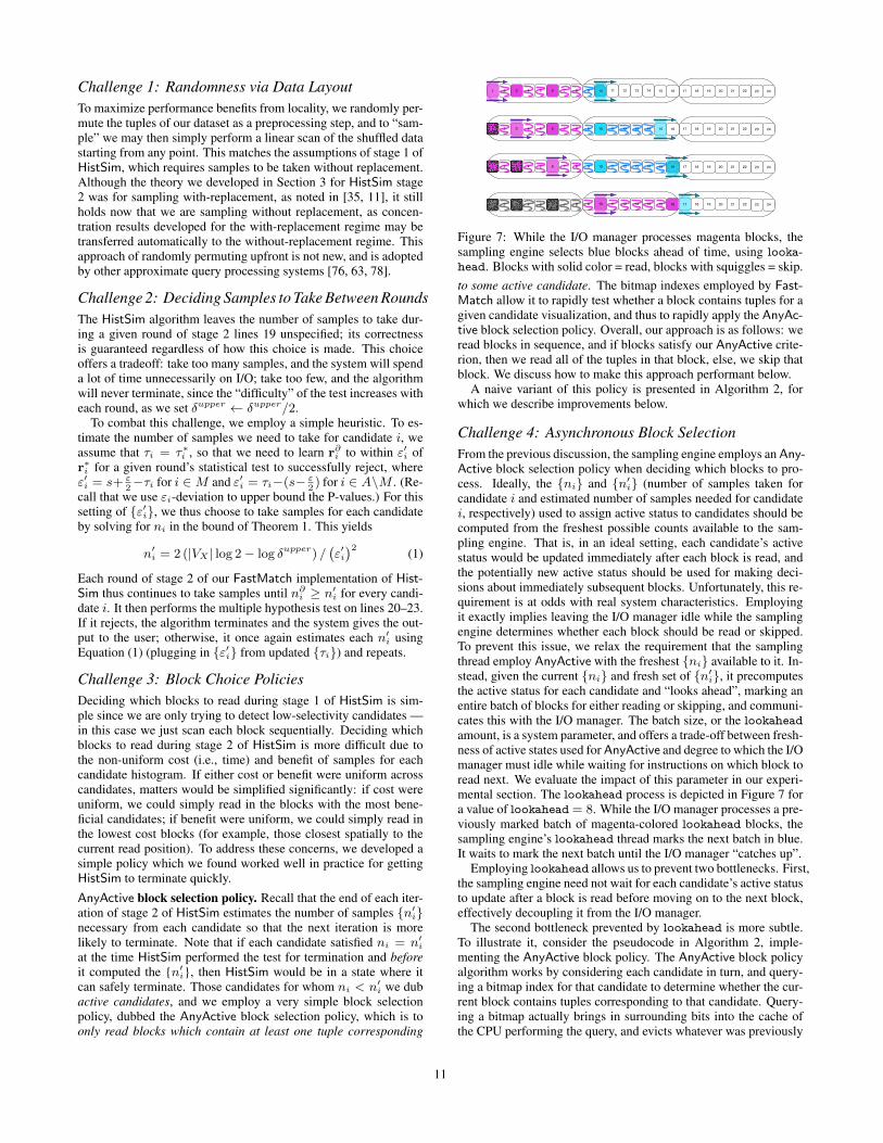
Challenge 4: Asynchronous Block SelectionFrom the previous discussion, the sampling engine employs an Any-Active block selection policy when deciding which blocks to pro-cess. Ideally, the ni and n′i (number of samples taken forcandidate i and estimated number of samples needed for candidatei, respectively) used to assign active status to candidates should becomputed from the freshest possible counts available to the sam-pling engine. That is, in an ideal setting, each candidate’s activestatus would be updated immediately after each block is read, andthe potentially new active status should be used for making deci-sions about immediately subsequent blocks. Unfortunately, this re-quirement is at odds with real system characteristics. Employingit exactly implies leaving the I/O manager idle while the samplingengine determines whether each block should be read or skipped.To prevent this issue, we relax the requirement that the samplingthread employ AnyActive with the freshest ni available to it. In-stead, given the current ni and fresh set of n′i, it precomputesthe active status for each candidate and “looks ahead”, marking anentire batch of blocks for either reading or skipping, and communi-cates this with the I/O manager. The batch size, or the lookaheadamount, is a system parameter, and offers a trade-off between fresh-ness of active states used for AnyActive and degree to which the I/Omanager must idle while waiting for instructions on which block toread next. We evaluate the impact of this parameter in our experi-mental section. The lookahead process is depicted in Figure 7 fora value of lookahead = 8. While the I/O manager processes a pre-viously marked batch of magenta-colored lookahead blocks, thesampling engine’s lookahead thread marks the next batch in blue.It waits to mark the next batch until the I/O manager “catches up”.

Employing lookahead allows us to prevent two bottlenecks. First,the sampling engine need not wait for each candidate’s active statusto update after a block is read before moving on to the next block,effectively decoupling it from the I/O manager.

The second bottleneck prevented by lookahead is more subtle.To illustrate it, consider the pseudocode in Algorithm 2, imple-menting the AnyActive block policy. The AnyActive block policyalgorithm works by considering each candidate in turn, and query-ing a bitmap index for that candidate to determine whether the cur-rent block contains tuples corresponding to that candidate. Query-ing a bitmap actually brings in surrounding bits into the cache ofthe CPU performing the query, and evicts whatever was previously

11

Algorithm 2: Naive AnyActive block processingInput : unpruned candidate set A, block index iOutput : A value indicating whether to :read or :skip block i

1 for each active cand ∈ A do// cache inefficient index lookup// evicts bits from previous candidate’s bitmap index

2 if cand.index_lookup(i) then3 return :read;4 end5 end6 return :skip;

Algorithm 3: AnyActive block selection with lookaheadInput : lookahead amount, start block, unpruned candidate set AOutput : An array mark indicating whether to :read or :skip blocks

// Initialization1 mark[i]← :skip for 0 ≤ i < lookahead;2 for each active cand ∈ A do3 for 0 ≤ i < lookahead do4 if mark[i] == :read then5 continue;6 else if cand.index_lookup(start + i) then7 mark[i]← :read;8 end9 end

10 end11 return mark

Dataset Size #Tuples #Attributes ReplicationsFLIGHTS 32 GiB 606 million 7 5×

TAXI 36 GiB 679 million 7 4×POLICE 34 GiB 448 million 10 72×

Table 2: Descriptions of Datasetsin the cache line. If blocks are processed individually, then onlya single bit in the bitmap is used each time a portion is broughtinto cache. This is quite wasteful and turns out to hurt performancesignificantly as we will see in the experiments. Instead, applyingAnyActive selection to lookahead-size chunks instead of individ-ual blocks is a better approach. This simply adds an extra inner loopto the procedure shown in Algorithm 2 (depicted in Algorithm 3).This approach has much better cache performance, since it uses anentire cache-line’s worth of bits while employing AnyActive.

We verify in our experiments that these optimizations allow Fast-Match to terminate more quickly via AnyActive block selectionwith fresh-enough active states without significantly slowing anysingle component of the system.

4.3 System ArchitectureFastMatch is implemented within a few thousand lines of C++.

It uses pthreads [59] for its threading implementation. FastMatchuses a column-oriented storage engine, as is common for analyticstasks. We can now complete our description of Figure 6. Whenthe I/O manager receives a request for a block at a particular blockindex from the sampling engine (via the “block index” message), iteventually returns a buffer containing the data at this block to thesampling engine (via the “buffer” message). Once the I/O phaseof stage 1 or 2 of HistSim completes, the sampling engine sendsthe current per-group counts for each candidate, ri, to the statis-tics engine. After running a test for whether to move to stage 2(performed in stage 1) or to terminate (performed in stage 2), thestatistics engine either posts a message of updated n′ (in stage 1)or n′i (stage 2) that the sampling engine uses to determine whento complete the I/O phase of each HistSim stage, as well as how toperform block selection during stage 2.

5. EXPERIMENTAL EVALUATIONThe goal of our experimental evaluation is to test the accuracy

and runtime of FastMatch against other approximate and exact ap-proaches on a diverse set of real datasets and queries. Furthermore,we want to validate the design decisions that we made for Fast-Match in Section 4 and evaluate their impact.

5.1 Datasets and QueriesWe evaluate FastMatch on publicly available real-world datasets

summarized in Table 2 — flight records [2], taxi trips [3], and po-lice road stops [4]. The replication value indicates how many times

each dataset was replicated to create a larger dataset. In prepro-cessing these datasets, we eliminated rows with “N/A” or erroneousvalues for any column appearing in one or more of our queries.FLIGHTS Dataset. Our FLIGHTS dataset, representing delays mea-sured for flights at more than 350 U.S. airports from 1987 up to2008, is available at [2]; we used 7 attributes (for origin / destina-tion airports, departure / arrival delays, day of week, day of month,and departure hour).TAXI Dataset. Our TAXI dataset summarizes all Yellow Cab tripsin New York in 2013 [3]. The subset of data we used correspondswith the urls ending in “yellow_tripdata_2013” in the file raw_-data_urls.txt. We extracted some time-based discrete attributes,two attributes based on passenger count, and one attribute based onarea, for 7 columns total. In particular, the “Location” attribute wasgenerated by binning the pickup location into regions of 0.01 lon-gitude by 0.01 latitude. As with our FLIGHTS data, we discardedrows with missing values, as well as rows with outlier longitudeor latitude values (which did not correspond to real locations). Thetaxi data stressed our algorithm’s ability to deal with low-selectivitycandidates, since more than 3000 candidates have fewer than 10 to-tal datapoints.POLICE Dataset. Our POLICE dataset summarizes more than 8million police road stops in Washington state [4]. We extracted at-tributes for county, two gender attributes, two race attributes, roadnumber, violation type, stop outcome, whether a search was con-ducted, and whether contraband was found, for 10 attributes total.Queries and Query Format. We evaluate several queries on eachdataset, whose templates are summarized in Table 3. We had fourqueries on FLIGHTS, FLIGHTS-q1-q4, two on TAXI, TAXI-q1-q2,and three on POLICE, POLICE-q1-q3. For simplicity, in all querieswe test, the x-axis is generated by grouping over a single attribute(denoted by “X” in Table 3), and the different candidates are like-wise generated by grouping over a single (different) attribute (sig-nified by “Z”). For each query, the visual target was chosen to cor-respond with the closest distribution (under `1) to uniform, out ofall histograms generated via the query’s template, except for q1,q2, and q3 of FLIGHTS. Our queries spanned a number of in-teresting dimensions: (i) frequently-appearing top-k candidates:FLIGHTS-q1, POLICE-q1 and q2, (ii) rarely-appearing top-k can-didates: FLIGHTS-q2 and q3, (iii) high-cardinality candidate at-tribute Z: TAXI-q1 and q2 (|VZ | = 7641), POLICE-q3 (|VZ | =2110), and (iv): high-cardinality grouping attribute X: FLIGHTS-q4 (|VX | = 351). The taxi queries in particular stressed our algo-rithm’s ability to deal with low-selectivity candidates, since morethan 3000 locations have fewer than 10 total datapoints.

5.2 Experimental Setup

12

Dataset Query Z (|VZ |) X (|VX |) k targetFLIGHTS q1 Origin (347) DepartureHour (24) 10 Chicago ORD

q2 Origin (347) DepartureHour (24) 10 Appleton ATWq3 Origin (347) DayOfWeek (7) 5 [0.25, 0.125, 0.125, 0.125, 0.125, 0.125, 0.125]q4 Origin (347) Dest (351) 10 closest candidate to uniform

TAXI q1 Location (7641) HourOfDay (24) 10 closest candidate to uniformq2 Location (7641) MonthOfYear (12) 10 closest candidate to uniform

POLICE q1 RoadID (210) ContrabandFound (2) 10 closest candidate to uniformq2 RoadID (210) OfficerRace (5) 10 closest candidate to uniformq3 Violation (2110) DriverGender (2) 5 closest candidate to uniform

Table 3: Summary of queries

Query Avg Speedup over Scan (raw time in (s))Scan(s) ScanMatch SyncMatch FastMatch

F-q1 12.26 27.74× (0.44) 25.53× (0.48) 37.52× (0.33)F-q2 12.29 3.17× (3.87) 2.73× (4.51) 10.11× (1.21)F-q3 11.62 4.76× (2.44) 3.14× (3.70) 8.72× (1.33)F-q4 13.97 5.93× (2.36) 5.76× (2.43) 8.15× (1.71)T-q1 13.09 4.89× (2.68) 0.32× (40.95) 15.93× (0.82)T-q2 13.09 6.48× (2.02) 0.37× (35.60) 17.38× (0.75)P-q1 8.57 5.72× (1.50) 5.14× (1.67) 13.34× (0.64)P-q2 8.49 14.31× (0.59) 15.48× (0.55) 36.11× (0.24)P-q3 8.65 9.25× (0.93) 1.53× (5.66) 33.26× (0.26)

Table 4: Summary of average query speedups and latencies

Approaches. We compare FastMatch against a number of lesssophisticated approaches that provide the same guarantee as Fast-Match. All approaches are parametrized by a minimum selectiv-ity threshold σ, and all approaches except Scan are additionallyparametrized by ε and δ and satisfy Guarantees 1 and 2 with prob-ability greater than 1− δ.• SyncMatch(ε, δ, σ). This approach uses FastMatch, but the

AnyActive block selection policy is applied without lookahead,synchronously and for each individual block. By comparingthis method with FastMatch, we quantify how much benefit wemay ascribe to the lookahead technique.

• ScanMatch(ε, δ, σ). This approach uses FastMatch, but with-out the AnyActive block selection policy. Instead, no blocksare pruned: it scans through each block in a sequential fashionuntil the statistics engine reports that HistSim’s termination cri-terion holds. By comparing this with SyncMatch, we quantifyhow much benefit we may ascribe to AnyActive block selection.

• Scan(σ). This approach is a simple heap scan over the entiredataset and always returns correct results, trivially satisfyingGuarantees 1 and 2. It exactly prunes candidates with selectiv-ity below σ. By comparing Scan with our above approximateapproaches, we quantify how much benefit we may ascribe tothe use of approximation.

Environment. Experiments were run on single Intel Xeon E5-2630 node with 125 GiB of RAM and with 8 physical cores (16logical) each running at 2.40 GHz, although we use at most 2 logi-cal cores to run FastMatch components. The Level 1, Level 2, andLevel 3 CPU cache sizes are, respectively: 512 KiB, 2048 KiB, and20480 KiB. We ran Linux with kernel version 2.6.32. We report re-sults for data stored in-memory, since the cost of main memoryhas decreased to the point that most interactive workloads can beperformed entirely in-core. Each run of FastMatch or any otherapproximate approach was started from a random position in theshuffled data. We report both wall clock times and accuracy as theaverage across 30 runs with identical parameters, with the excep-tion of Scan, whose wall clock times we report as the average over5 runs. Where applicable, we used default settings ofm = 5 ·105,δ = 0.01, ε = 0.04, σ = 0.0008, and lookahead = 1024. Weset the block size for each column to 600 bytes, which we found toperform well; our results are not too sensitive to this choice.

5.3 MetricsWe use several metrics to compare FastMatch against our base-

lines in order to test two hypotheses: one, that FastMatch does

indeed provide accurate answers, and two, that the system architec-ture developed in Section 4 does indeed allow for earlier termina-tion while satisfying the separation and reconstruction guarantees.Wall-Clock Time. Our primary metric evaluates the end-to-endtime of our approximate approaches that are variants of FastMatch,as well as a scan-based baseline.Satisfaction of Guarantees Guarantee 1 and Guarantee 2. Ourδ parameter (δ = 0.01), serves as an upper bound on the probabil-ity that either of these guarantees are violated. If this bound weretight, we would expect to see about one run in every hundred fail tosatisfy our guarantees. We therefore count the number of times ourguarantees are violated relative to the number of queries performed.Total Relative Error in Visual Distance. In some situations, theremay be several candidate histograms that are quite close to theanalyst-supplied target, and choosing any one of them to be amongthe k returned to the analyst would be a good choice. We define thetotal relative error in visual distance (denoted by ∆d) between thek candidates returned by FastMatch and the true k closest visual-

izations as: ∆d(M,M∗,q) =∑i∈M d(ri,q)−

∑j∈M∗ d(r

∗j ,q)∑

j∈M∗ d(r∗j ,q)

Note

that here, M∗ is computed by Scan and only considers candidatesmeeting the selectivity threshold. Since FastMatch and our otherapproximate variants have no recall requirements with respect toidentifying low-selectivity candidates (they only have precision re-quirements), it is possible for ∆d < 0.

5.4 Empirical ResultsSpeedups and Error of FastMatch versus others.

Summary. All FastMatch variants we tested show signif-icant speedups over Scan for at least one query, but onlyFastMatch shows consistently excellent performance, typicallybeating other approaches and bringing latencies for all queriesnear interactive levels; with an overall speedup ranging between8× and 35× over Scan. Further, the output of FastMatch andall approximate variants satisfied Guarantees 1 and 2 acrossall runs for all queries.Average run times of FastMatch and other approaches, for all

queries as well as speedups over Scan, are summarized in Table 4.We used default settings for all runs. The reported speedups are theratio of the average wall time of Scan with the average wall timeof each approach considered. Scan was generally slower than ap-proximate approaches because it had to examine all the data. Then,we typically observed that ScanMatch and SyncMatch were prettyevenly matched, with ScanMatch usually performing slightly bet-ter, except in some pathological cases where it performed verypoorly due to poor cache usage. FastMatch had better performancethan either SyncMatch or ScanMatch, thanks to lookahead pairedwith AnyActive block selection. Overall, we observed that each ofFastMatch’s key innovations: the termination criterion, the blockselection, and lookahead, all led to substantial performance im-provements, with an overall speedup of up to 35× over Scan.

Queries with high candidate cardinality (TAXI-q*, POLICE-q3),displayed particularly interesting performance differences. For these,FastMatch shows greatly improved performance over ScanMatch.

13

0.02 0.03 0.04 0.05 0.06 0.07 0.08 0.09 0.10 0.11

0.0

0.5

1.0

1.5

flights-q1

0.02 0.03 0.04 0.05 0.06 0.07 0.08 0.09 0.10 0.11

0

5

10

flights-q2

0.02 0.03 0.04 0.05 0.06 0.07 0.08 0.09 0.10 0.11

0

5

10

flights-q3

0.02 0.03 0.04 0.05 0.06 0.07 0.08 0.09 0.10 0.11

0

2

4

6

8

wal

ltim

e(s

)

flights-q4

0.02 0.03 0.04 0.05 0.06 0.07 0.08 0.09 0.10 0.11

0.0

2.5

5.0

7.5

taxi-q1 (SYNCMATCH not shown)

0.02 0.03 0.04 0.05 0.06 0.07 0.08 0.09 0.10 0.11

0

2

4

6

taxi-q2 (SYNCMATCH not shown)

0.02 0.03 0.04 0.05 0.06 0.07 0.08 0.09 0.10 0.11

0

2

4

6police-q1

0.02 0.03 0.04 0.05 0.06 0.07 0.08 0.09 0.10 0.11

ε (at δ=0.01)

0

1

2

police-q2

0.02 0.03 0.04 0.05 0.06 0.07 0.08 0.09 0.10 0.11

0

5

10

15

20police-q3

FASTMATCH SYNCMATCH SCANMATCH

Figure 8: Effect of ε on query latency

It also scales much better to the large number of candidates thanSyncMatch, which performs extremely poorly due to poor cacheutilization and takes around 3× longer than a simple non-approximateScan. In this case, the lookahead technique of FastMatch is nec-essary to reap the benefits of AnyActive block selection.

Additionally, we found that the output of FastMatch and all ap-proximate variants satisfied Guarantees 1 and 2 across all runs forall queries. This suggests that the parameter δ may be a loose upperbound for the actual failure probability of FastMatch.Effect of varying ε.

Summary. In almost all cases, increasing the tolerance parame-ter ε leads to reduced runtime and accuracy, but on average, ∆d

was never more than 5% larger than optimal for any query,even for the largest values of ε used.Figures 8 and 9 depict the effect of varying ε on the wall clock

time and on ∆d, respectively, using δ = 0.01 and lookahead =1024, averaged over 30 runs for each value of ε. Because of theextremely poor performance of SyncMatch on the TAXI queries,we omit it from both figures.

In general, as we increased ε, wall clock time decreased and ∆d

increased. In some cases, ScanMatch latencies matched that ofScan until we made ε large enough. This sometimes happenedwhen it needed more refined estimates of the (relatively infrequent)top-k candidates, which it achieved by scanning most of the data,picking up lots of superfluous (in terms of achieving safe termina-tion) tuples along the way.Effect of varying lookahead.

Summary. When the number of candidates |VZ | is not large,performance is relatively stable as lookahead varies. For large|VZ |, more lookahead helps performance, but is not crucial.For most queries, we found that latency was relatively robust to

changes in lookahead. Figure 10 depicts this effect. The querieswith high candidate cardinalities (TAXI-q*, POLICE-q3) were theexceptions. For these queries, larger lookahead values led to in-creased utilization at all levels of CPU cache. Past a certain point,however, the performance gains were minor. Overall, we found thedefault value of 1024 to be acceptable in all circumstances.Effect of varying δ. In general, we found that increasing δ led toslight decreases in wall clock time, leaving accuracy (in terms of

Query |M∗(`1)∩M∗(`2)|k

Relative distance differenceFLIGHTS-q1 0.9 0.01FLIGHTS-q2 0.7 0.04FLIGHTS-q3 0.6 0.03FLIGHTS-q4 0.8 0.01Table 5: Comparison of top-closest histograms for `1 and `2

∆d) more or less constant. We believe this behavior is inheritedfrom our bound in Theorem 1, which is not sensitive to changes inδ. Figure 11 shows the effect of varying δ on wall clock time. Forthe values of δ we tried, we did not observe any meaningful trendsin ∆d and have omitted the plot.When approximation performs poorly. In order to achieve thecompetitive results presented in this section, the initial pruning oflow-selectivity candidates during stage 1 of HistSim ended up be-ing critical for good performance. With a selectivity threshold ofσ = 0, stages 2 and 3 of HistSim are forced to consider many ex-tremely rare candidates. For example, in the taxi queries, nearlyhalf of candidates have fewer than 10 corresponding datapoints. Inthis case, ScanMatch performs the best (essentially performing aScan with a slight amount of additional overhead), but it (necessar-ily) fails to take enough samples to establish Guarantees 1 and 2.SyncMatch and FastMatch likewise fail to establish guarantees,but additionally have the issue of being forced to consider manyrare candidates while employing AnyActive block selection, whichcan slow town query processing by a factor of 100× or more.Comparing results for `1 and `2 metrics. So far, we have notvalidated our choice of distance metric (normalized `1); prior workhas shown that normalized `2 is suitable for assessing the “visual”similarity of visualizations [71], so here, we compare our top-kwith the top-k using the normalized `2 metric, for the FLIGHTSqueries. In brief, we found that the relative difference in the total`1 distance of the top-k using the two metrics never exceeded 4%for any query, and that roughly 75% of the top-k candidates werecommon across the two metrics. Thus, `1 can serve as a suitablereplacement for `2, while further benefiting from the advantageswe described in Section 2. Table 5 summarizes our full results.

6. RELATED WORKWe now briefly cover work that is related to FastMatch from a

number of different areas.

14

0.02 0.03 0.04 0.05 0.06 0.07 0.08 0.09 0.10 0.11

0.000

0.001

0.002

0.003

flights-q1

0.02 0.03 0.04 0.05 0.06 0.07 0.08 0.09 0.10 0.11

0.00000

0.00025

0.00050

0.00075

0.00100

flights-q2

0.02 0.03 0.04 0.05 0.06 0.07 0.08 0.09 0.10 0.11

0.000

0.005

0.010

0.015flights-q3

0.02 0.03 0.04 0.05 0.06 0.07 0.08 0.09 0.10 0.11

−0.050

−0.025

0.000

0.025

0.050

∆d

flights-q4

0.02 0.03 0.04 0.05 0.06 0.07 0.08 0.09 0.10 0.11

−0.035

−0.030

−0.025taxi-q1 (SYNCMATCH not shown)

0.02 0.03 0.04 0.05 0.06 0.07 0.08 0.09 0.10 0.11

0.00

0.02

0.04

taxi-q2 (SYNCMATCH not shown)

0.02 0.03 0.04 0.05 0.06 0.07 0.08 0.09 0.10 0.11

−0.01

0.00

0.01

0.02

0.03police-q1

0.02 0.03 0.04 0.05 0.06 0.07 0.08 0.09 0.10 0.11

ε (at δ=0.01)

−0.0090

−0.0085

−0.0080

police-q2

0.02 0.03 0.04 0.05 0.06 0.07 0.08 0.09 0.10 0.11

0.000

0.002

0.004

0.006

police-q3

FASTMATCH SYNCMATCH SCANMATCH

Figure 9: Effect of ε on ∆d

23 25 27 29 2110.0

0.5

1.0

1.5

2.0

wal

ltim

e(s

)

flights queries

flights-q1 flights-q2 flights-q3

23 25 27 29 211

lookahead

0

5

10

taxi queries

taxi-q1 taxi-q2

23 25 27 29 2110.0

0.5

1.0

1.5

police queries

police-q1 police-q2 police-q3

Figure 10: Effect of varying lookahead

Approximate Query Processing (AQP). Offline AQP involves com-puting a set of samples offline, and then using these samples whenqueries arrive e.g., [40, 21, 5, 9, 7], with systems like BlinkDB [7]and Aqua [6]. These techniques crucially rely on the availabilityof a workload. On the other hand, online approximate query pro-cessing, e.g., [34, 37, 53], performs sampling on-the-fly, typicallyusing an index to facilitate the identification of appropriate sam-ples. Our work falls into the latter category; however, none of theprior work has addressed a similar problem of identifying relevantvisualizations given a query.

Top-K or Nearest Neighbor Query Processing. There is a vastbody of work on top-k query processing [38]. Most of this workrelies on exact answers, as opposed to approximate answers, andhas different objectives. As an example, Bruno et al. [16] exploitstatistics maintained by a RDBMS in order to quickly find top-ktuples matching user-specified attribute values. Some work triesto bridge the gap between top-k query processing and uncertainquery processing [69, 65, 68, 25, 61, 23, 49, 14], but does not needto deal with the concerns of where and when to sample to returnanswers quickly, but approximately. Some of this work [69, 65,49, 14] develops efficient algorithms for top-k or nearest neighborsin a uncertain databases setting—here, the sampling is restrictedto monte-carlo sampling, which is very different in behavior. Sil-berstein et al. [68] retain samples of past sensor readings to avoidmaintaining joint probability distributions in a sensor network. Co-hen et al. [25] develops techniques to bound the probability of agiven set of items being part of the top-k. Pietracaprina et al. [61]develops sampling schemes tailored to finding top-k frequent item-sets. Chen et al. [23] employ sampling to determine the bounds of

a minimum bounding rectangle for top-k nearest neighbor queries.Zhang et al. [79] performs top-k similarity search efficiently in anetwork context.

Scalable Visualizations. There has been some limited work onscalable approximate visualizations, targeting the generation of asingle visualization, while preserving certain properties [46, 60,64]. In our setting, the space of sampling is much larger—as aresult the problem is more complex. Furthermore, the objectivesare very different. Fisher et al. [30] explores the impact of ap-proximate visualizations on users, adopting an online-aggregation-like [34] scheme. As such, these papers show that users are ableto interpret and utilize approximate visualizations correctly. Somework uses pre-materialization for the purpose of displaying visu-alizations quickly [44, 51, 55]; however, these techniques rely onin-memory data cubes. We covered other work on scalable visual-ization via approximation [28, 57, 43, 60, 77, 71] in Section 1.

Histogram Estimation for Query Optimization. A number ofrelated papers [22, 39, 41] are concerned with the problem of sam-pling for histogram estimation, usually for estimating attribute valueselectivities [52] and query size estimation (see [24] for a recentexample). While some of the theoretical tools used are similar, theproblem is fundamentally different, in that the aforementioned lineof work is concerned with estimating one histogram per table orview for query optimization purposes with low error, while we areconcerned with comparing histograms to a specific target.

Sublinear Time Algorithms. HistSim is related to work on sub-linear time algorithms—the most relevant ones [12, 20, 72] fallunder the setting of distribution learning and analysis of property

15

0.01 0.02

0.0

0.2

0.4

flights-q1

0.01 0.02

0

2

4

flights-q2

0.01 0.02

0

1

2

3

4

flights-q3

0.01 0.02

0

1

2

wal

ltim

e(s

)

flights-q4

0.01 0.02

0

1

2

taxi-q1 (SYNCMATCH not shown)

0.01 0.02

0

1

2

taxi-q2 (SYNCMATCH not shown)

0.01 0.02

0.0

0.5

1.0

1.5

2.0police-q1

0.01 0.02

δ (at ε=0.04)

0.0

0.2

0.4

0.6

0.8police-q2

0.01 0.02

0

2

4

6police-q3

FASTMATCH SYNCMATCH SCANMATCH

Figure 11: Effect of δ on wall clock time

testers for whether distributions are close under `1 distance. Al-though Chan et al. [20] develop bounds for testing whether distri-butions are ε-close in the `1 metric, property testers can only saywhen two distributions p and q are equal or ε-far, and cannot handle||p− q||1 < ε for p 6= q, a necessary component of this work.

7. CONCLUSION AND FUTURE WORKWe developed sampling-based strategies for rapidly identifying

the top-k histograms that are closest to a target. We designed a gen-eral algorithm, HistSim, that provides a principled framework tofacilitate this search, with theoretical guarantees. We showed howthe systems-level optimizations present in our FastMatch architec-ture are crucial for achieving near-interactive latencies consistently,leading to speedups ranging from 8× to 35× over baselines. Whilethis work suggests several possible avenues for further exploration,we are particularly interested in exploring the impact of our sys-tems architecture in supporting general interactive analysis.

8. REFERENCES[1] Boost Statistical Distributions and Functions.

https://www.boost.org/doc/libs/1_67_0/libs/math/doc/html/dist.html, 2006.

[2] Flight Records. http://stat-computing.org/dataexpo/2009/the-data.html,2009.

[3] NYC Taxi Trip Records.https://github.com/toddwschneider/nyc-taxi-data/,2015.

[4] WA Police Stop Records.https://stacks.stanford.edu/file/druid:py883nd2578/WA-clean.csv.gz, 2017.

[5] S. Acharya, P. B. Gibbons, and V. Poosala. Congressionalsamples for approximate answering of group-by queries. InACM SIGMOD Record, volume 29, pages 487–498. ACM,2000.

[6] S. Acharya, P. B. Gibbons, V. Poosala, and S. Ramaswamy.The aqua approximate query answering system. In ACMSigmod Record, volume 28, pages 574–576. ACM, 1999.

[7] S. Agarwal, B. Mozafari, A. Panda, H. Milner, S. Madden,and I. Stoica. Blinkdb: Queries with bounded errors andbounded response times on very large data. In EuroSys,pages 29–42, New York, NY, USA, 2013. ACM.

[8] D. Alabi and E. Wu. Pfunk-h: approximate query processingusing perceptual models. In HILDA@ SIGMOD, page 10,2016.

[9] N. Alon, Y. Matias, and M. Szegedy. The space complexityof approximating the frequency moments. In STOC, pages20–29. ACM, 1996.

[10] B. Babcock, S. Chaudhuri, and G. Das. Dynamic sampleselection for approximate query processing. In SIGMOD,New York, New York, USA, 2003.

[11] R. Bardenet, O.-A. Maillard, et al. Concentration inequalitiesfor sampling without replacement. Bernoulli,21(3):1361–1385, 2015.

[12] T. Batu, L. Fortnow, R. Rubinfeld, W. D. Smith, andP. White. Testing that distributions are close. In FOCS, 2000.

[13] J. T. Behrens. Principles and procedures of exploratory dataanalysis. Psychological Methods, 2(2):131, 1997.

[14] G. Beskales, M. A. Soliman, and I. F. Ilyas. Efficient searchfor the top-k probable nearest neighbors in uncertaindatabases. Proceedings of the VLDB Endowment,1(1):326–339, 2008.

[15] M. Bostock, V. Ogievetsky, and J. Heer. D3 data-drivendocuments. IEEE TVCG, 17(12):2301–2309, 2011.

[16] N. Bruno, S. Chaudhuri, and L. Gravano. Top-k selectionqueries over relational databases: Mapping strategies andperformance evaluation. ACM TODS, 27(2):153–187, June2002.

[17] G. Casella and R. L. Berger. Statistical inference, volume 2.Duxbury Pacific Grove, CA, 2002.

[18] K. Chakrabarti, M. Garofalakis, R. Rastogi, and K. Shim.Approximate query processing using wavelets. The VLDBJournal, 10(2-3):199–223, Sept. 2001.

[19] C.-Y. Chan and Y. E. Ioannidis. Bitmap index design andevaluation. In ACM SIGMOD Record, volume 27, pages355–366. ACM, 1998.

16

[20] S.-O. Chan, I. Diakonikolas, G. Valiant, and P. Valiant.Optimal algorithms for testing closeness of discretedistributions. In SODA, pages 1193–1203, 2014.

[21] S. Chaudhuri, G. Das, M. Datar, R. Motwani, andV. Narasayya. Overcoming limitations of sampling foraggregation queries. In ICDE, pages 534–542. IEEE, 2001.

[22] S. Chaudhuri, R. Motwani, and V. Narasayya. Randomsampling for histogram construction: How much is enough?In ACM SIGMOD Record, volume 27, pages 436–447.ACM, 1998.

[23] C.-M. Chen and Y. Ling. A sampling-based estimator fortop-k selection query. In Data Engineering, 2002.Proceedings. 18th International Conference on, pages617–627. IEEE, 2002.

[24] Y. Chen and K. Yi. Two-level sampling for join sizeestimation. In Proceedings of the 2017 ACM InternationalConference on Management of Data, pages 759–774. ACM,2017.

[25] E. Cohen, N. Grossaug, and H. Kaplan. Processing top-kqueries from samples. Computer Networks,52(14):2605–2622, 2008.

[26] C. Daskalakis, I. Diakonikolas, R. ODonnell, R. A. Servedio,and L.-Y. Tan. Learning sums of independent integer randomvariables. In FOCS, pages 217–226. IEEE, 2013.

[27] I. Diakonikolas. Personal communication, 2017.[28] B. Ding, S. Huang, S. Chaudhuri, K. Chakrabarti, and

C. Wang. Sample + seek: Approximating aggregates withdistribution precision guarantee. In SIGMOD, 2016.

[29] M. El-Hindi, Z. Zhao, C. Binnig, and T. Kraska. Vistrees:fast indexes for interactive data exploration. In Proceedingsof the Workshop on Human-In-the-Loop Data Analytics,page 5. ACM, 2016.

[30] D. Fisher, I. Popov, S. Drucker, and m.c. Schraefel. Trust me,i’m partially right. In CHI, page 1673, New York, New York,USA, may 2012. ACM Press.

[31] V. Ganti, M.-L. Lee, and R. Ramakrishnan. Icicles:Self-tuning samples for approximate query answering. InVLDB, volume 176, 2000.

[32] A. L. Gibbs and F. E. Su. On choosing and boundingprobability metrics. International statistical review,70(3):419–435, 2002.

[33] P. Hanrahan. Analytic database technologies for a new kindof user: The data enthusiast. In SIGMOD, pages 577–578,New York, NY, USA, 2012. ACM.

[34] J. M. Hellerstein, P. J. Haas, and H. J. Wang. Onlineaggregation. ACM SIGMOD Record, 26(2):171–182, jun1997.

[35] W. Hoeffding. Probability inequalities for sums of boundedrandom variables. Journal of the American statisticalassociation, 58(301):13–30, 1963.

[36] S. Holm. A simple sequentially rejective multiple testprocedure. Scandinavian journal of statistics, pages 65–70,1979.

[37] W.-C. Hou, G. Ozsoyoglu, and B. K. Taneja. Processingaggregate relational queries with hard time constraints. InACM SIGMOD Record, volume 18, pages 68–77. ACM,1989.

[38] I. F. Ilyas, G. Beskales, and M. A. Soliman. A survey oftop-k query processing techniques in relational databasesystems. ACM Comput. Surv., 40(4), 2008.

[39] Y. E. Ioannidis and V. Poosala. Balancing histogramoptimality and practicality for query result size estimation. InACM SIGMOD Record, volume 24, pages 233–244. ACM,

1995.[40] Y. E. Ioannidis and V. Poosala. Histogram-based

approximation of set-valued query-answers. In VLDB,volume 99, pages 174–185, 1999.

[41] H. V. Jagadish, N. Koudas, S. Muthukrishnan, V. Poosala,K. C. Sevcik, and T. Suel. Optimal histograms with qualityguarantees. In VLDB, volume 98, pages 24–27, 1998.

[42] N. L. Johnson, A. W. Kemp, and S. Kotz. Univariate discretedistributions, volume 444. John Wiley & Sons, 2005.

[43] U. Jugel, Z. Jerzak, G. Hackenbroich, and V. Markl. M4: avisualization-oriented time series data aggregation. PVLDB,7(10):797–808, 2014.

[44] S. Kandel, R. Parikh, A. Paepcke, J. M. Hellerstein, andJ. Heer. Profiler: Integrated statistical analysis andvisualization for data quality assessment. In AVI, pages547–554. ACM, 2012.

[45] M. S. Kester, M. Athanassoulis, and S. Idreos. Access pathselection in main-memory optimized data systems: Should iscan or should i probe? In Proceedings of the 2017 ACMInternational Conference on Management of Data, pages715–730. ACM, 2017.

[46] A. Kim, E. Blais, A. Parameswaran, P. Indyk, S. Madden,and R. Rubinfeld. Rapid sampling for visualizations withordering guarantees. PVLDB, 8(5):521–532, Jan. 2015.

[47] A. Kim, S. Madden, and A. Parameswaran. Needletail: Asystem for browsing queries (demo). Technical report,Available at:http://i.stanford.edu/~adityagp/ntail-demo.pdf ,2014.

[48] A. Kim, L. Xu, T. Siddiqui, S. Huang, S. Madden, andA. Parameswaran. Optimally leveraging density and localityto support limit queries. Technical report, Available at:https://arxiv.org/pdf/1611.04705.pdf , 2016.

[49] H.-P. Kriegel, P. Kunath, and M. Renz. Probabilisticnearest-neighbor query on uncertain objects. Advances indatabases: concepts, systems and applications, pages337–348, 2007.

[50] E. L. Lehmann and J. P. Romano. Testing statisticalhypotheses. Springer Science & Business Media, 2006.

[51] L. D. Lins, J. T. Klosowski, and C. E. Scheidegger.Nanocubes for real-time exploration of spatiotemporaldatasets. IEEE TVCG, 19(12):2456–2465, 2013.

[52] R. J. Lipton, J. F. Naughton, and D. A. Schneider. Practicalselectivity estimation through adaptive sampling, volume 19.ACM, 1990.

[53] R. J. Lipton, J. F. Naughton, D. A. Schneider, andS. Seshadri. Efficient sampling strategies for relationaldatabase operations. Theoretical Computer Science,116(1):195–226, 1993.

[54] Z. Liu and J. Heer. The effects of interactive latency onexploratory visual analysis. IEEE TVCG, 20(12):2122–2131,2014.

[55] Z. Liu, B. Jiang, and J. Heer. immens: Real-time visualquerying of big data. In CGF, volume 32, pages 421–430.Wiley Online Library, 2013.

[56] C. McDiarmid. On the method of bounded differences.Surveys in combinatorics, 141(1):148–188, 1989.

[57] D. Moritz, D. Fisher, B. Ding, and C. Wang. Trust, butverify: Optimistic visualizations of approximate queries forexploring big data. In CHI, pages 2904–2915. ACM, 2017.

[58] B. Mozafari. Approximate query engines: Commercialchallenges and research opportunities. In SIGMOD, pages

17

521–524. ACM, 2017.[59] B. Nichols, D. Buttlar, and J. Farrell. Pthreads programming:

A POSIX standard for better multiprocessing. " O’ReillyMedia, Inc.", 1996.

[60] Y. Park, M. Cafarella, and B. Mozafari. Visualization-awaresampling for very large databases. In ICDE, pages 755–766.IEEE, 2016.

[61] A. Pietracaprina, M. Riondato, E. Upfal, and F. Vandin.Mining top-k frequent itemsets through progressivesampling. Data Mining and Knowledge Discovery,21(2):310–326, 2010.

[62] P. Pirolli and S. Card. The sensemaking process and leveragepoints for analyst technology as identified through cognitivetask analysis. In Proceedings of international conference onintelligence analysis, volume 5, pages 2–4, 2005.

[63] C. Qin and F. Rusu. Pf-ola: a high-performance frameworkfor parallel online aggregation. Distributed and ParallelDatabases, 32(3):337–375, 2014.

[64] S. Rahman, M. Aliakbarpour, H. K. Kong, E. Blais,K. Karahalios, A. Parameswaran, and R. Rubinfield. I’veseen “enough”: Incrementally improving visualizations tosupport rapid decision making. In VLDB, 2017.

[65] C. Ré, N. N. Dalvi, and D. Suciu. Efficient top-k queryevaluation on probabilistic data. In ICDE, pages 886–895,2007.

[66] P. G. Selinger, M. M. Astrahan, D. D. Chamberlin, R. A.Lorie, and T. G. Price. Access path selection in a relationaldatabase management system. In Proceedings of the 1979ACM SIGMOD international conference on Management ofdata, pages 23–34. ACM, 1979.

[67] T. Siddiqui, A. Kim, J. Lee, K. Karahalios, andA. Parameswaran. Effortless data exploration with zenvisage:an expressive and interactive visual analytics system.PVLDB, 10(4):457–468, 2016.

[68] A. S. Silberstein, R. Braynard, C. Ellis, K. Munagala, andJ. Yang. A sampling-based approach to optimizing top-kqueries in sensor networks. In Data Engineering, 2006.ICDE’06. Proceedings of the 22nd International Conferenceon, pages 68–68. IEEE, 2006.

[69] M. A. Soliman, I. F. Ilyas, and K. C. Chang. Top-k queryprocessing in uncertain databases. In ICDE, pages 896–905,2007.

[70] C. Stolte, D. Tang, and P. Hanrahan. Polaris: A system forquery, analysis, and visualization of multidimensionalrelational databases. IEEE TVCG, 8(1):52–65, 2002.

[71] M. Vartak, S. Rahman, S. Madden, A. Parameswaran, andN. Polyzotis. Seedb: efficient data-driven visualizationrecommendations to support visual analytics. PVLDB,8(13):2182–2193, 2015.

[72] B. Waggoner. L p testing and learning of discretedistributions. In ITCS, pages 347–356. ACM, 2015.

[73] H. Wickham. ggplot2: elegant graphics for data analysis.Springer, 2016.

[74] K. Wu, E. Otoo, and A. Shoshani. Compressed bitmapindices for efficient query processing. Lawrence BerkeleyNational Laboratory, 2001.

[75] K. Wu, K. Stockinger, and A. Shoshani. Breaking the curseof cardinality on bitmap indexes. In Scientific and StatisticalDatabase Management, pages 348–365. Springer, 2008.

[76] S. Wu, B. C. Ooi, and K.-L. Tan. Continuous sampling foronline aggregation over multiple queries. In SIGMOD, pages651–662. ACM, 2010.

[77] Y. Wu, B. Harb, J. Yang, and C. Yu. Efficient evaluation ofobject-centric exploration queries for visualization. PVLDB,8(12):1752–1763, 2015.

[78] K. Zeng, S. Agarwal, A. Dave, M. Armbrust, and I. Stoica.G-ola: Generalized on-line aggregation for interactiveanalysis on big data. In SIGMOD, pages 913–918. ACM,2015.

[79] J. Zhang, J. Tang, C. Ma, H. Tong, Y. Jing, J. Li, W. Luyten,and M.-F. Moens. Fast and flexible top-k similarity search onlarge networks. ACM Transactions on Information Systems(TOIS), 36(2):13, 2017.

APPENDIXA. EXTENSIONS

A.1 Generalizing Problem Description

A.1.1 SUM aggregationsWhile we do not consider it explicitly in this paper, in [28],

the authors describe how to perform SUM aggregations with `2distributional guarantees via measure-biased sampling. Briefly, ameasured-biased sample for some attribute Y involves samplingeach tuple t in T , where the probability of inclusion in the sam-ple is proportional t’s value of Y . FastMatch can also leveragemeasure-biased samples in order to match bar graphs generated viathe following types of queries:

SELECT X , SUM(Y) FROM TWHERE Z = zi GROUP BY X

As in Definition 1, Z is the candidate attribute and X is the group-ing attribute for the x-axis. One measure-biased sample must becreated per measure attribute Y the analyst is interested in, so ifthere are n such attributes, we require an additional n completepasses over the data for preprocessing. When matching bar graphsgenerated according to the above template, FastMatch would sim-ply use the measure-biased sample for Y and pretend as if it werematching visualizations generated according to Definition 1; thatis, it would use COUNT instead of SUM. There is nothing spe-cial about the `2 metric used in [28], and the same techniques maybe used by FastMatch to process queries satisfying Guarantees 1and 2.

A.1.2 Candidates based off arbitrary boolean predi-cates

In order to support candidates based off boolean predicates suchas Z(1) = z

(1)i ∧Z

(2) = z(2)j , FastMatch needs a way to estimate

the number of active tuples in a block for the purposes of apply-ing AnyActive block selection. In this case, simple bitmap indexeswith one bit per block are not enough. We may instead opt to usethe slightly costlier density maps from [48]. We refer readers tothat paper for a description of how to estimate the number of tuplesin a block satisfying an arbitrary boolean predicate. Even if differ-ent candidates share some of the same tuples, our guarantees stillhold since HistSim uses a Holm-Bonferroni procedure to get jointguarantees across different candidates at a given iteration, a methodwhich is agnostic to any dependency structure between candidates.

A.1.3 Multiple attributes in GROUP BY clauseIn the case where the analyst wishes to use multiple attributes

X(1), X(2), . . . , X(n) to generate the support of our histogramsgenerated via Definition 1, all of the same methods apply, but weestimate the support |VX | as

|VX(1) | · |VX(2) | · . . . · |VX(n) |

18

This may be an overestimate if two attribute values, say x(1)i andx(2)j , never occur together. Our guarantees still hold in this case

— overestimating the size of the support can only make the boundin Theorem 1 looser than it could be, which does not cause anycorrectness issues.

A.1.4 Handling continuous X attributes via binningIf the analyst wishes to use a continuousX , she must simply pro-

vide a set of non-overlapping bin ranges, or “buckets” in which tocollect tuples. Everything else is still the same. In fact, FLIGHTS-q1 and FLIGHTS-q2 used this technique, since the DepartureHourattribute was actually a continuous attribute we placed into 24 bins(although we presented it as a discrete attribute for simplicity).

A.1.5 Handling an Unknown Candidate DomainIf the candidate domain is unknown at query time, for example

if we do not have any bitmap index structures over the attribute(s)used to generate candidates, it is still possible to use a variant of ourmethods. First of all, we may still employ ScanMatch, creatingstate for new candidates as they are discovered. During stage 1 ofHistSim, in which rare candidates are pruned, we must also accountfor any potential candidates for which HistSim has not yet seen anytuples. In this case, we may simply add one additional “dummy”candidate which matches against all the tuples for any unseen can-didates. We add an additional test to the Holm-Bonferroni proce-dure for this dummy candidate — if the test rejects, and if U repre-sents the indices of the unseen candidates, then we can be sure that∑j∈U NjN

< σ, which in turn implies that NjN< σ for each j ∈ U .

A.1.6 Handling Continuous CandidatesIf one or more of the attributes used to group candidates is con-

tinuous, then, as in the case of continuous X , candidates may be“grouped” by placing different real-values into bins. We can alsoconstruct bitmaps for continuous attributes at some predetermined

finest level of granularity of binning, which can then be used to in-duce bitmaps for any coarser granularity that may be needed. Evenif the finest granularity available is too coarse to isolate differentcandidates, as long as it isolates some subsets of candidates, it maystill be useful for pruning the blocks that need to be considered forAnyActive block selection. Even if there is no index available, onemay still use ScanMatch.

A.2 Different Types of Guarantees

A.2.1 Allowing Distinct ε1 and ε2 for Guarantees 1and 2

If the analyst believes one of Guarantees 1 and 2 is more impor-tant than the other, she may indicate this by providing separate ε1for Guarantee 1 and ε2 for Guarantee 2; HistSim generalizes in avery straightforward way in this case. For example, if Guarantee 2is more important than Guarantee 1, the analyst may provide ε1 andε2 with ε2 < ε1.

A.2.2 Allowing other distance metricsWe can extend HistSim to work for any distance metric for which

there exists an analogue to Theorem 1. For example, there existsuch bounds for `2 distance [28, 72].

A.2.3 Allowing a range of k in inputIn some cases, the analyst may not care about the exact number

of matching candidates. For example, the analyst may be fine withfinding anywhere between 5 and 10 of the closest histograms to atarget. In this case, she may specify a range [k1, k2], and Fast-Match may return some number k ∈ [k1, k2] of histograms match-ing the target, where k is automatically picked to make it as easyas possible to satisfy Guarantees 1 and 2. For example, in the case[k1, k2] = [5, 10], there may be a very large separation betweenthe 7th- and 8th-closest candidates, in which case HistSim can au-tomatically choose k = 7, as this likely provides a small δupper assoon as possible.

19