adaptive random linear network coding with controlled
TRANSCRIPT

Adaptive Random Linear Network Coding with Controlled
Forwarding for Wireless Broadcast
by
Kashif Mahmood
A thesis submitted to The Faculty of Graduate Studies and Research
in partial fulfilment of the degree requirements of
Master of Applied Science in Electrical and Computer Engineering
Ottawa-Carleton Institute for Electrical & Computer Engineering Department of Systems and Computer Engineering
Carleton University Ottawa, Ontario, Canada
December 2010
© Copyright 2010, Kashif Mahmood

1*1 Library and Archives Canada
Published Heritage Branch
395 Wellington Street OttawaONK1A0N4 Canada
Bibliotheque et Archives Canada
Direction du Patrimoine de I'edition
395, rue Wellington OttawaONK1A0N4 Canada
Your file Votre reference ISBN: 978-0-494-79542-2 Our file Notre reference ISBN: 978-0-494-79542-2
NOTICE: AVIS:
The author has granted a nonexclusive license allowing Library and Archives Canada to reproduce, publish, archive, preserve, conserve, communicate to the public by telecommunication or on the Internet, loan, distribute and sell theses worldwide, for commercial or noncommercial purposes, in microform, paper, electronic and/or any other formats.
L'auteur a accorde une licence non exclusive permettant a la Bibliotheque et Archives Canada de reproduire, publier, archiver, sauvegarder, conserver, transmettre au public par telecommunication ou par I'lnternet, preter, distribuer et vendre des theses partout dans le monde, a des fins commerciales ou autres, sur support microforme, papier, electronique et/ou autres formats.
The author retains copyright ownership and moral rights in this thesis. Neither the thesis nor substantial extracts from it may be printed or otherwise reproduced without the author's permission.
L'auteur conserve la propriete du droit d'auteur et des droits moraux qui protege cette these. Ni la these ni des extraits substantiels de celle-ci ne doivent etre imprimes ou autrement reproduits sans son autorisation.
In compliance with the Canadian Privacy Act some supporting forms may have been removed from this thesis.
Conformement a la loi canadienne sur la protection de la vie privee, quelques formulaires secondaires ont ete enleves de cette these.
While these forms may be included in the document page count, their removal does not represent any loss of content from the thesis.
Bien que ces formulaires aient inclus dans la pagination, il n'y aura aucun contenu manquant.
1+1
Canada
Abstract
Multicasting and broadcasting are important communication techniques in
wireless adhoc networks. Recently, Network Coding (NC), which has emerged as a
promising technique for various applications, has been applied to multicast and broadcast
in wireless adhoc networks. It is however observed that the performance using NC is
strongly dependent upon the topology, node density and the kind of coding algorithm.
The algorithms that are proposed are mostly dealing with single source multicasting or
broadcasting.
In this thesis I propose an adaptive multi-source broadcasting protocol using
Random Linear Network Coding (RLNC). The key features of this protocol include its
multi-source operation, cross-session generations, controlling the number of re
transmissions effectively based on neighbourhood information and earlier decoding. Our
simulations with and without cross-session generations show that cross-session
generations result in improved Packet Delivery Ratio as well as lower latency. We also
investigate its adaptive performance compared to packet forwarding schemes, including a
simple flooding protocol, a probabilistic flooding protocol, BCAST and Simplified
Multicast Forwarding. We observe the steady performance of our protocol under different
node densities and rates.
n

Dedicated to my parents, my wife and my wonderful son
in

Acknowledgements
I would like to express my sincere gratitude to my advisors, Dr. Thomas Kunz
and Dr. Ashraf Matrawy for their extraordinary support and guidance throughout my
graduate studies at Carleton University. I must unequivocally acknowledge that Dr.
Thomas was a real source of motivation for me and there was not a single moment when
I found myself unguided. He was always available with his valuable suggestions and
guidance throughout my thesis. Dr. Ashraf was also always motivating and supported me
on quite a few occasions where I was in a fix.
I also would like to thank my friends and colleagues who were always there to
extend support and motivation. I would like to thank the SCE department and overall the
Carleton University for all their support. This work was partially funded by
Communication Research Center (CRC), Canada and I would like to thank CRC for their
support. I also would like thank the Graduate Chair for all his moral and financial
support.
Not to mention, I would like to especially thank my parents whose prayers are
always there for me and it's due to their prayers and efforts which have led me to success
in life. I would like to thank my wife and son, who were always there to support me in all
circumstances and situations. As a student with minimal resources and no time for
family, she was always there as a support. Finally, I would like to thank my sister and
brother-in-law who always motivated me and guided me on all occasions during the
research work.

Table of Contents
Chapter 1 Introduction 1
1.1 Background 1
1.2 Emergence of Network Coding for Wireless Networks 1
1.3 Problem Statement 2
1.4 Proposed Scheme 4
1.5 Thesis Organization 5
Chapter 2 Network Coding 6
2.1 Concept 6
2.2 Types of Network Coding 7
2.2.1 XOR-basedNC 7
2.2.2 Reed-Solomon-based NC 10
2.2.3 Random Linear Network Coding 12
2.3 Benefits of Network Coding 14
Chapter 3 Related Work 17
3.1 Broadcast Media 17
3.2 Efficient Packet-Forwarding-Based Wireless Broadcast 18
3.3 Related Work on RLNC for Wireless Networks 20
3.3.1 Analytical Work 20
v

3.3.2 RLNC-based Heuristic Protocols 26
3.4 Discussion 31
Chapter 4 Proposed Model 34
4.1 Adaptive Random Linear Network Coding with Controlled Forwarding
(ARLNCCF) 34
4.2 Proposed Scheme 34
4.2.1 Hello Control Messages and Number of Retransmissions 36
4.2.2 Packet Format 37
4.2.3 Generation Size 39
4.2.4 Generation Timeout 40
4.2.5 Generation Distance (GD) 40
4.2.6 Partial and Full Decoding 41
4.2.7 Generation ID - Duplication 42
4.3 Operation of ARLNCCF 42
4.3.1 Source Node Operation 43
4.3.2 Intermediate Node Operation 45
4.3.3 Decoding Process 51
Chapter 5 Simulation Setup 55
5.1 Simulation Tool & Parameters 55
5.2 Performance Metrics 56
vi

5.3 Algorithms for Comparison 58
5.4 Sensitivity of ARLNCCF 60
5.4.1 Generation Size 60
5.4.2 Generation Timeout 67
5.4.3 Early Decoding 71
5.5 Simulation Scenarios 77
5.5.1 Wi-Fi Scenarios 77
5.5.2 Tactical Scenarios 81
Chapter 6 Adaptive Performance 84
6.1 Static Scenarios 01-Source 84
6.2 Static Scenarios 04-Sources 91
6.3 Mobile Scenarios 01-Source 96
6.4 Mobile Scenarios 04-Sources 102
6.5 Tactical Scenarios 01-Source 106
6.6 Tactical Scenarios 04-Sources 108
6.7 Summary 110
Chapter 7 Cross-Session Performance 114
7.1 100-source scenarios 114
7.2 4-Source Scenarios 116
Chapter 8 Conclusions and Future Work 121
vii

8.1 Conclusions 121
8.2 Future Work 123
Appendix A 132
Vll l

List of Figures
Figure 2.1: Basic NC idea [19] 6
Figure 2.2: Butterfly Network without NC 7
Figure 2.3: Butterfly Network with NC 8
Figure 2.4: Data Forwarding without and with COPE [20] 9
Figure 2.5: RS Codeword 10
Figure 2.6: RLNC Process 12
Figure 3.1: Dominating Set (DS) & Connected Dominating Set (CDS) 19
Figure 4.1: Neighborhood of Node m 37
Figure 4.2: Packet Format for ARLNCCF 38
Figure 4.3: Flow Diagram of GD Concept 41
Figure 4.4: Flow Diagram - Encoding Process 43
Figure 4.5: Single Packet Insertion 45
Figure 4.6: Flow Diagram - Intermediate Node Operation 46
Figure 4.7: Generation with Symbol Location and Respective Coding Coefficients 48
Figure 4.8: Received Packet with Symbol Location and Respective Coefficients 49
Figure 4.9: Generation 73098 after Conflict Resolution 49
Figure 4.10: Generation 73098 with Symbol Location and Respective Symbols 50
Figure 4.11: Received Packet for Generation 73098 51
Figure 4.12: Generation 73098 after Conflict Resolution 51
Figure 4.13: Flow Diagram - Decoding Process 52
Figure 4.14: Earlier Decoding Examples 53
Figure 5.1: PDRvs. Generation Size (01 Source) 61
ix

Figure 5.2: Latency vs. Generation Size (01 Source) 62
Figure 5.3: PDR vs. Generation Size (04 Sources) 63
Figure 5.4: Latency vs. Generation Size (04 Sources) 64
Figure 5.5: MAC Transmissions vs. Generation Size (04 Sources) 66
Figure 5.6: PDR vs. Generation Timeout 68
Figure 5.7: Latency vs. Generation Timeout 70
Figure 5.8: MAC Transmissions vs. Generation Timeout 70
Figure 5.9: PDR vs. Rate (kbps) - (Static - 01 Source) 71
Figure 5.10: Latency vs. Rate (kbps) - (Static - 01 Source) 72
Figure 5.11: PDR vs. Nodes (Static - 01 Source) 73
Figure 5.12: Latency vs. Nodes (Static - 01 Source) 74
Figure 5.13: PDR vs. Rate (kbps) - (Static - 04 Source) 75
Figure 5.14: Latency vs. Rate (kbps) - (Static - 04 Source) 75
Figure 5.15: PDR vs. Nodes (Static - 0 4 Sources) 76
Figure 5.16: Latency vs. Nodes (Static - 04 Sources) 77
Figure 5.17: Different Scenarios 78
Figure 6.1: PDR vs. Rate (kbps) - (Static - 01 Source) 85
Figure 6.2: Latency vs. Rate (kbps) - (Static - 01 Source) 86
Figure 6.3: MAC Transmissions vs. Rate (kbps) - (Static - 01 Source) 86
Figure 6.4: IFQ Drops vs. Rate (kbps) - (Static - 01 Source) 87
Figure 6.5: PDR vs. Nodes (Static - 01 Source) 88
Figure 6.6: Latency vs. Nodes (Static - 01 Source) 89
Figure 6.7: MAC Transmissions vs. Nodes (Static - 01 Source) 89
x

Figure 6.8: IFQ Drops vs. Nodes (Static - 01 Source) 90
Figure 6.9: PDR vs. Rate (kbps) - (Static - 04 Sources) 91
Figure 6.10: Latency vs. Rate (kbps) - (Static - 04 Sources) 92
Figure 6.11: MAC Transmissions vs. Rate (kbps) - (Static - 04 Sources) 92
Figure 6.12: IFQ Drops vs. Rate (kbps) - (Static - 04 Sources) 93
Figure 6.13: PDR vs. Nodes (Static - 04 Sources) 94
Figure 6.14: Latency vs. Nodes (Static - 04 Sources) 95
Figure 6.15: MAC Transmissions vs. Nodes (Static - 04 Sources) 95
Figure 6.16: IFQ Drops vs. Nodes (Static - 04 Sources) 96
Figure 6.17: PDR vs. Rate (kbps) - (Mobility - 01 Source) 97
Figure 6.18: Latency vs. Rate (kbps) - (Mobility - 01 Source) 97
Figure 6.19: MAC Transmissions vs. Rate (kbps) - (Mobility - 01 Source) 98
Figure 6.20: IFQ Drops vs. Rate (kbps) - (Mobility - 01 Source) 98
Figure 6.21: PDR vs. Nodes - (Mobility - 01 Source) 100
Figure 6.22: Latency vs. Nodes - (Mobility - 01 Source) 100
Figure 6.23: MAC Transmissions vs. Nodes - (Mobility - 01 Source) 101
Figure 6.24: IFQ Drops vs. Nodes - (Mobility - 01 Source) 101
Figure 6.25: PDR vs. Rate (kbps) - (Mobility - 04 Sources) 102
Figure 6.26: Latency vs. Rate (kbps) - (Mobility-04 Sources) 103
Figure 6.27: MAC Transmissions vs. Rate (kbps) - (Mobility - 04 Sources) 103
Figure 6.28: IFQ Drops vs. Rate (kbps) - (Mobility - 04 Sources) 104
Figure 6.29: PDR vs. Nodes - (Mobility - 04 Sources) 104
Figure 6.30: Latency vs. Nodes - (Mobility - 04 Sources) 105
xi
Figure 6.31: MAC Transmissions vs. Nodes - (Mobility - 04 Sources) 105
Figure 6.32: IFQ Drops vs. Nodes - (Mobility - 04 Sources) 106
Figure 6.33: PDR vs. Rate (kbps) - (Tactical - 01 Source) 107
Figure 6.34: Latency vs. Rate (kbps) - (Tactical - 01 Source) 107
Figure 6.35: MAC Transmissions vs. Rate (kbps) - (Tactical - 01 Source) 108
Figure 6.36: PDR vs. Rate (kbps) - (Tactical - 04 Sources) 109
Figure 6.37: Latency vs. Rate (kbps) - (Tactical - 04 Sources) 109
Figure 6.38: MAC Transmissions vs. Rate (kbps) - (Tactical - 04 Sources) 110
Figure 7.1: PDR vs. Rate (kbps) - (04 Sources) 117
Figure 7.2: Latency vs. Rate (kbps) - (04 Sources) 117
Figure 7.3: PDR vs. Nodes - (04 Sources) 118
Figure 7.4: Latency vs. Nodes (04 Sources) 119
Figure A.l: Encoding Process 132
xii

List of Tables
Table 4.1: Notations used in the Algorithm 42
Table 5.1: Default values in NS2 55
Table 5.2: Optimal P values used for Probabilistic Flooding 59
Table 5.3: Common Parameters 79
Table 5.4: Simulation Parameters 80
Table 5.5: Simulation Parameters 81
Table 6.1: Comparing SMF and ARLNCCF for Wi-Fi and Tactical Scenarios 111
Table 7.1: PDR for 1 Packet and 4 Packets per Source 115
Table 7.2: Latency for 1 Packet and 4 Packets per Source 116
Table 7.3: Confidence Interval-PDR (04 Sources - 50 Nodes) 118
Table 7.4: Confidence Interval-Latency (04 Sources - 50 Nodes) 119
Table A.l Simplified Multiplication on GF (28) 135
xm
List of Acronyms
AES: Advanced Encryption Standard
ARLNCCF: Adaptive Random Linear Network Coding with Controlled Forwarding
ARQ: Automatic Repeat reQuest
ARQ-E: Enhanced ARQ
ARQ-SPR: Single Path Routing ARQ
BCAST: No Acronym
CBR: Constant Bit Rate
CDS: Connected Dominating Set
DS: Dominating Set
DTN: Delay Tolerant Networks
FEC: Forward Error Correction
GD: Generation Distance
GF: Galois Field
MANETs: Mobile Adhoc NETworks
MC2: Multipath Code Casting
MPR: Multi Point Relay
NC: Network Coding
OLSR: Optimized Link State Routing protocol
OMNC: Optimized Multipath Network Coding
PDR: Packet Delivery Ratio
RLNC: Random Linear Network Coding
RS: Reed-Solomon
xiv

SMF: Simplified Multicast Forwarding
S-MPR: Source based Multi Point Replay
TBRPF: Topology dissemination Based on Reverse-Path Forwarding
xv

Chapter 1
Introduction
1.1 Background
In many wireless applications, there is a requirement to flood information to all
the nodes in the network with one-to-many or many-to-many communication patterns to
disseminate control messages and other important information like emergency messages
in battlefield operation and disaster relief operations, etc. Simple flooding, in which each
node in the network rebroadcasts the packet it receives, requires no overhead but
consumes lots of channel bandwidth as many duplicate packets are received by the nodes.
The result, called broadcast storm [1], causes significant packet loss and network
congestion.
In order to deal with the broadcast storm problem, more efficient ways have been
proposed for broadcasting in multi-hop wireless networks by reducing the number of
redundant retransmissions. Various techniques have been applied to reduce the number of
retransmissions (i.e. number of nodes forwarding the broadcast packets) in wireless
networks while attempting to ensure that a broadcast packet is delivered to each node in
the network. The detailed explanation of these techniques is provided in Chapter 3.
1.2 Emergence of Network Coding for Wireless Networks
Wireless networks, which are basically broadcast in nature, have some potential
challenges compared to wired networks. The challenges include low throughput, limited
1

bandwidth, dead spots, poor performance under mobility, energy-constrained operation,
unreliability, susceptible to environmental factors such as fading and interference, and
security threats. However, the inherent characteristics of wireless media like its broadcast
nature, the diversity of information and data redundancy can help in designing new ways
of wireless communication [2]. One emerging area, originally designed for wired
networks, is Network Coding (NC) [3] that works very well in wireless broadcast
environment by exploiting these characteristics. With network coding, the sending nodes
or the intermediate nodes not only act as relay but they additionally combine (encode) a
number of packets they have received into one or several outgoing packets, thus
improving the throughput of the network. Various analytical models and simulations have
shown that network coding can improve the efficiency, throughput, complexity,
robustness and security of the network [4] [5] [6].
Various NC based techniques have been proposed and applied to applications like
multicasting and broadcasting in wireless networks, peer to peer file distribution [7],
security and robustness to attacks [8], video surveillance [9], as an alternative to
Automatic Repeat reQuest (ARQ) [10], large scale content distribution [11], on chip
communication [12] and distributed storage [13]. A more detailed explanation of these
techniques is given in Chapter 2.
1.3 Problem Statement
In simple packet forwarding, if the packet is lost, there is no way to recover the
lost packet unless the source sends that packet again or same packet is overheard from
another neighbour (opportunistic listening). Using network coding, nodes are allowed to
2
process (encode / re-encode) the received incoming packets instead of simply forwarding
or repeating them. Thus, the packets which are independently generated by the source
nodes are not required to be processed separately by intermediate nodes. These packets
can be combined into one or several outgoing packets. If the encoded packet is lost, there
is still a chance that if the required number of encoded packets can be collected by a node
from any neighbour or group of neighbours, the original packets can be recovered
without any retransmission from the source node. Due to this appealing property, network
coding is able to offer benefits in various aspects of communication networks. The
benefits of using NC are discussed in detail in Chapter 2.
Consideration of the benefits of NC motivated us to explore its potential for
wireless broadcasting. Although there are many proposed schemes dealing with single
source wireless broadcast using NC, only few works are related to multi-source
broadcast. Similarly, the protocol performance depends on how it adapts to the different
data rates and node densities. Many existing protocols have parameters that can be set to
appropriate values like probability of retransmission or forwarding factor [14][15] to
adapt themselves to the above situations. We would like a solution where the protocol is
able to adapt itself automatically, thus, making it more suitable for wireless adhoc
networks.
In this thesis, we have developed a NC-based broadcast protocol that works well
for both single-source and multi-source environment. We have explored the potential
benefit of allowing packets originating from different sources to be combined/coded
together, as opposed to the already proposed algorithms that limit this to packets
originating from the same source only (detail is provided in later chapters). We have
3

shown through simulations that our protocol is able to adapt well to different nodes
densities and data rates and show steady performance in terms of Packet Delivery Ratio
(PDR) and end-to-end packet delay.
1.4 Proposed Scheme
Our main focus is the application of NC in the area of broadcasting in wireless
adhoc networks. Various analytical models have been proposed and their performance is
evaluated [16] [17]. Our proposed scheme uses Random Linear Network Coding (RLNC)
for wireless broadcast. We call it Adaptive Random Linear Network Coding with
Controlled Forwarding (ARLNCCF). Very little work addresses the issue of multi-source
RLNC-based broadcast [16]. The key elements of our protocol are as following.
1. The algorithm is specifically designed to work in multi-source broadcast
environments. The scheme works well for both single-source and multi-source
environments by allowing to code/combine packets originating from different
sources. This improves the Packet Delivery Ratio and reduces the latency.
2. Using neighbour knowledge and the generation size, our scheme can effectively
calculate the number of rebroadcasts that are sufficient for all the nodes to decode the
coded packets. Hence, it is adaptive to varying nodes densities, making it more
suitable for adhoc networks in which there is no control over the number and density
of nodes in the network.
3. The Generation Distance (GD) concept is introduced to check the size of generation
to grow uncontrolled in a multi-source environment.
4
4. An early decoding concept, which is also considered in some of the other research
papers, is included in our protocol. We have used different possibilities of early
decoding to enhance the performance of our protocol. We have investigated the
performance of with and without early decoding. This investigation is not done so far
in the research.
Based on our research work, a paper was published in International Federation for
Information Processing (IFIP) / IEEE Wireless Days (WD'10) Conference [18] held in
Venice in October 2010.
1.5 Thesis Organization
This thesis is organized in the following manner. Chapter 2 is discussing various
NC algorithms and their implementation detail. It also covers some of the benefits of NC
mentioned in the literature. Chapter 3 deals with the application of RLNC to wireless
adhoc networks. The main focus is on the algorithms and analytical models proposed so
far, dealing with multicasting and broadcasting. This chapter also briefly reviews packet
forwarding broadcast protocols. Chapter 4 discusses our proposed model and its
implementation detail. Chapter 5 discusses the sensitivity of our protocol as well as the
simulation setup. Chapter 6 is related to the performance evaluation and comparison of
our protocol to the other selected protocols. Chapter 7 discusses the cross-session
performance of our protocol and finally Chapter 8 is related to the conclusion and future
work.
5
Chapter 2
Network Coding
2.1 Concept
Network Coding is a relatively new concept in information theory. Unlike the
existing store and forward routing schemes, in which data is relayed hop by hop from a
source to a destination without being altered, NC refers to the notion of mixing (linearly
combining) information from different flows at intermediate nodes in the network. The
receiver decodes these packets to recover the original data when it receives enough coded
packets. It has been shown that multicast capacity can be achieved by mixing packets
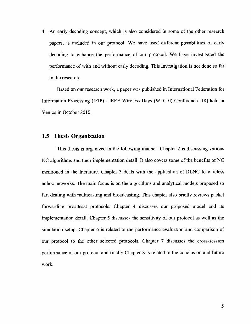
from different flows [3]. As shown in Figure 2.1, each node in a network can perform
some computation and output packets are a function of input packets. Intuitively, network
coding allows information to be mixed at a node.
/l(Vl>V2,V3)
'/IOV^)
Figure 2.1: Basic NC idea [19]
6

Coding Gain
In terms of NC, coding gain is the effective gain that NC provides over non-coded
packets. The gain can be in terms of Packet Delivery Ratio (PDR), reliability, robustness,
number of transmissions or lower end-to-end latency of packets etc.
2.2 Types of Network Coding
There are various types of NC that have been applied in the research. NC can be
classified into the following three types.
1) XOR-based
2) Reed-Solomon-based
3) Random Linear Network Coding (RLNC)
Each of the above types is explained in detail in the following sections.
2.2.1 XOR-based NC
XOR-based algorithms are the simplest algorithm to encode the data packets. The
benefit of XOR-based NC is very well explained in the literature using the famous
Butterfly Network for wired networks by Ahlswede et al [3]. The coding gain can be
explained as follows:
Figure 2.2: Butterfly Network without NC
7

Refer to Figure 2.2; it is the case of a butterfly network without NC. The source S
wants to multicast two bits bi and b2 to two receivers Y and Z. Let us assumes that the
capacity of each link is 1 bit per second. The source S sends bi through link S - T and b2
through link S - U as two bits cannot be sent together through the same link at the same
time. If we use the standard store and forward scheme, the middle link W - X cannot
transmit two bits at the same time. W sends the two bits alternately. Now if we calculate
the throughput at each receiver, it will not be 2 bits/sec but 1.5 bits/sec due to the limited
capacity of link W - X.
I b.ffl b,
b.e^Q^)^® b.
or ^ ©
Figure 2.3: Butterfly Network with NC
Refer to Figure 2.3 now, it shows the case of the same network using XOR-based
NC. The node W has enough processing power to linearly combine the two bits it has
received by calculating the XOR operation i.e. bi © b2. The XOR-ed version is forwarded
to node X, which broadcasts the same to the destination nodes Y and Z. Meanwhile, Y
receives bi from the T - Y link and Z receives b2 from the U - Z link.
The decoding is done in a very simple way at the destination nodes. Node Y is
able to decode b2 by b2 = bi© (bi © b2). Similarly, node Z is able to decode bi by bi = b2
8

© (bi © b2). If we calculate the throughput, it will be 2 bits/sec. This simple example
clearly shows improvement in the throughput of the network using NC.
The slight overhead that can be seen here is the buffer space requirement as well
as additional processing in encoding and decoding the packet. With the advancement in
solid states like high speed processors and high speed and large capacity memories, these
overheads are well taken care of. The bandwidth is limited especially in wireless
networks. Using NC, we can efficiently utilize the bandwidth of the network.
The above example is for a wired network. Another example of XOR-based
coding, this time in a wireless broadcast network, is provided in the work of Katti et al.
[20] and shown in Figure 2.4. They proposed the COPE algorithm, using XOR-based
NC. If node A wants to send a message to node B (and vice versa) and there is an
intermediate node / router R between them that relays the messages between A and B, the
process requires 4 transmissions in total. On the other hand, if A and B send their packets
to R and R broadcasts the XOR version of the packet, a total of 3 transmissions are
required. In this case, node A and B can obtain each other's packets by XOR-ing them
with their own packets.
" i 1 ~ d A ' C ? . . - - ' S ?- . . 2 B J
R ' 1 ~~ -* 2
*"-.£5 " I
GO; Mmg
Figure 2.4: Data Forwarding without and with COPE [20]
c?-
9
2.2.2 Reed-Solomon-based NC
Reed-Solomon (RS) codes are block-based error correcting codes with a wide
range of applications in digital communications and storage. Reed-Solomon codes are
used to correct errors in many systems which include [21]:
• Storage devices (including tape, Compact Disk, DVD, barcodes, etc)
• Wireless or mobile communications (including cellular telephones, microwave
links, etc)
• Satellite communications
• Digital Video / DVB
• High-speed modems such as ADSL, xDSL, etc.
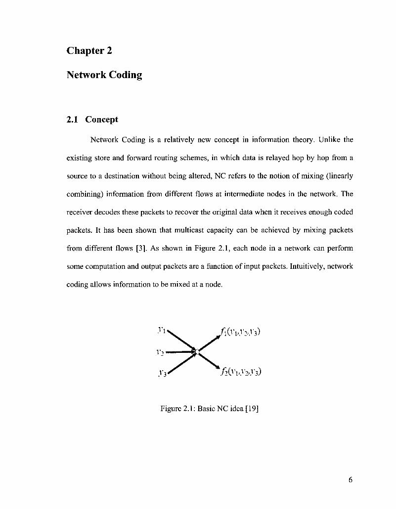
A Reed-Solomon code is specified as RS (n,k) with 5-bit symbols. This means
that the encoder takes k data symbols of s bits each and adds parity symbols to generate
an n symbol codeword. There are n-k parity symbols of s bits each. A Reed-Solomon
decoder can correct up to t symbols that contain errors in a codeword, where 2t = n-k.
The following diagram shows a typical Reed-Solomon codeword (this is known as a
systematic code because the data is left unchanged and the parity symbols are appended).
n
DATA s, _J
PARITY ^ J
V
Figure 2.5: RS Codeword
10

Example: A popular RS code is RS (255,223) with 8-bit symbols. Each codeword
contains n = 255 code word bytes, of which k = 223 bytes are data and 2t = n-k = 32
bytes are parity. If the locations of the symbols in error are not known in advance, then a
Reed-Solomon code can correct up to t = (n - k) I 2 erroneous symbols, i.e., it can
correct half as many errors as there are redundant symbols added to the block. This
implies t = 16. The decoder can correct any 16 symbol errors in the code word: i.e. errors
in up to 16 bytes anywhere in the codeword can be automatically corrected.
Sometimes error locations are known in advance (e.g., "side information" in
demodulator signal-to-noise ratios)—these are called erasures. A Reed-Solomon code is
able to correct twice as many erasures as errors, and any combination of errors and
erasures can be corrected as long as the relation 2E + S < = n-k is satisfied, where E is the
number of errors and S is the number of erasures in the block.
RS-code-based NC is used for broadcasting in Mobile AdHoc Networks
(MANETS) in [22]. The authors claimed to achieve 61% coding gain compared to a non-
coding approach. The authors defined coding gain as the ratio of the number of
transmission required by a specific non-coding approach, to the number of transmissions
used by their protocol to deliver the same set of packets to all nodes. However the results
are greatly dependent upon the network topology and density of the network. As this
protocol extensively relies upon opportunistic listening, sparsely placed nodes do not get
much chance of overhearing other messages.
The proposed algorithm works as follows. Let u be the source, v be the receiver
where v e N(u). N(u) is the set of neighbors of node u. Assume that P is the ordered set
of n native packets in u 's output queue. Once u broadcasts the coded packets P, let Pv be
11
the set of packets received by node v, for each v e N(u). Let k = max {\P — Pv\, v e
N{u)} and 0 be the k * n Vandermonde matrix which represents RS codes. Then the
minimal number of encoded packets that needs to be sent, such that each neighbor v can
decode the packets in P - Pv is k and the set of k packets are given by Q = 0 x P.
Therefore a node constructs the coded packet set Q = 0 xP. It then adds the set of native
packet IDs to each coded packet and the index number of codes used. When a node v
receives an encoded packet consisting of n native packets (set P), v first goes over all
native packets received in its packet pool. It collects Pv, the subset of packets in P that it
has already received. It then constructs Av (the decoding matrix) and adds the new
coefficient vector to matrix Av. For each decoded native packet q, node v can now
process q.
2.2.3 Random Linear Network Coding
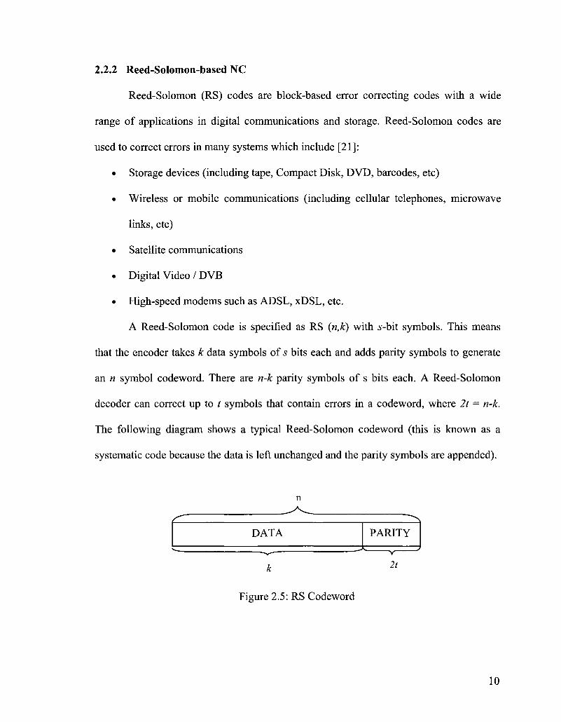
In case of Random Linear Network Coding [23], the output flow at the given node
is obtained as a linear combination of its input flows. The coefficients selected for this
linear combination are completely random in nature, hence the name Random Linear
Network Coding (RLNC). The node combines a number of packets it has received or
created into one or several outgoing coded packets.
Coding coefficients Coding coefficients
Original packet— i j >» Encoder
\ 7 Encoded packet \ 7 Re-encoded packet
£ > Re-encoder £ > Decoder
Original packet
Intermediate nodes
Figure 2.6: RLNC Process
12
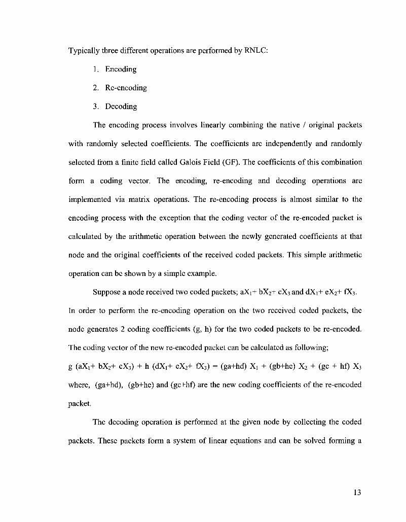
Typically three different operations are performed by RNLC:
1. Encoding
2. Re-encoding
3. Decoding
The encoding process involves linearly combining the native / original packets
with randomly selected coefficients. The coefficients are independently and randomly
selected from a finite field called Galois Field (GF). The coefficients of this combination
form a coding vector. The encoding, re-encoding and decoding operations are
implemented via matrix operations. The re-encoding process is almost similar to the
encoding process with the exception that the coding vector of the re-encoded packet is
calculated by the arithmetic operation between the newly generated coefficients at that
node and the original coefficients of the received coded packets. This simple arithmetic
operation can be shown by a simple example.
Suppose a node received two coded packets; aXi+ bX2+ CX3 and dXi+ eX2+ 1X3.
In order to perform the re-encoding operation on the two received coded packets, the
node generates 2 coding coefficients (g, h) for the two coded packets to be re-encoded.
The coding vector of the new re-encoded packet can be calculated as following;
g (aXi+ bX2+ cX3) + h (dXi+ eX2+ fX3) = (ga+hd) Xi + (gb+he) X2 + (gc + hf) X3
where, (ga+hd), (gb+he) and (gc+hf) are the new coding coefficients of the re-encoded
packet.
The decoding operation is performed at the given node by collecting the coded
packets. These packets form a system of linear equations and can be solved forming a
13
matrix. The matrix is referred to as decoding matrix. Appendix A contains a detailed
description of the encoding, re-encoding and decoding processes.
• Generation
It is important to limit the size of the matrix that is used for encoding and
decoding. For that purpose the packets are grouped together in blocks. Each block is
called a Generation. Only packets of the same generation can be encoded and later
decoded. It is shown that the size and composition of the generation has significant
impact on the performance of network coding [24].
• Dependency
It is shown that with RLNC, there exists a probability of selecting linearly
dependant combinations, which depends upon the size of the GF, i.e., the range of
possible coding coefficient values. However, it is shown through simulations that, even
choosing a small field size, this probability becomes negligible [8].
• Rank of a Matrix
The rank of a matrix is the maximum number of independent rows (or the
maximum number of independent columns) of a matrix.
• Innovative Packet
A packet is said to be innovative if it increases the rank of a matrix.
2.3 Benefits of Network Coding
Some of the benefits of using NC for wireless networks are mentioned in [2] [8].
14

Throughput
As mentioned before, NC increases the capacity of a network for multicast flows.
It is shown in the literature that, using NC, the same information is delivered while
transmitting fewer packets in the network. In case of flooding, the broadcast storm
overwhelms the network bandwidth. NC is an effective way to deal with this problem in a
distributed way for multicasting and broadcasting [20][23][25].
Reliability
Some of the main advantages of NC include higher reliability [10] and robustness
[14], especially in case of mobile and lossy networks, where other FEC or ARQ schemes
do not show good performance. By encoding the packets into a single packet, we are
ensuring that a single packet loss does not necessarily require retransmissions [26]. If the
complete set of coded packets of the same generation can be received from any node,
decoding can be successful and all the packets can be recovered. Similarly, the concept of
partial decoding is also provided in the literature where partial packets can still be
recovered even if all the required encoded packets are not received.
Distributed Nature
With NC, there is no need to have global knowledge of the network. Especially in
case of RLNC, we even do not care what the neighbour has received. It is highly
distributed in nature. Due to this property it is well suited for wireless networks which are
also distributed in nature.
Low Complexity
Overall, NC works by solving the set of equations linearly combined together in
polynomial time. The decoding is performed using Gaussian elimination methods. These
15

methods are simple in computation and utilize the cheap computational power to improve
network efficiency [16] [24].
Mobility
In mobile environments, the network topology changes over time and a main
difficulty for many routing protocols are the frequent route updates and gathering new
topological information. NC can address this uncertainty and alleviate the need for
exchanging route updates [9] [14].
Security
Sending the linear combination of the packets instead of un-coded packets offers a
natural way to take advantage of multipath diversity for security against wiretapping
attacks in wireless networks [27].
16
Chapter 3
Related Work
3.1 Broadcast Media
As mentioned earlier, wireless media, which is broadcast in nature, is a very
suitable candidate for NC. As a result, researchers have explored its benefit for wireless
networks, especially wireless adhoc networks (both static and mobile). Due to the adhoc
nature of the networks, each node is capable of generating as well as routing / relaying
the packets in the network from other nodes.
NC performance is strongly relying on diversity of information, which in the case
of wireless networks can significantly improve the performance of multicast and
broadcast messages in adhoc networks. The wireless media is unreliable and lossy. There
can be frequent retransmissions as required by standard error detection and correction
schemes like Forward Error Correction (FEC) and Automatic Repeat reQuest (ARQ).
Secondly, in case of broadcasting, reliable broadcast requires that every receiver must
receive the correct information sent by the sender. In case of wireless adhoc networks,
which are infrastructure-less with limited bandwidth, simple flooding causes bandwidth
bottlenecks and loss of packets. Finding more effective ways to multicast and broadcast
messages has always been a challenging task and many new protocols and algorithms
have been proposed. In this chapter we will focus on the current research trends dealing
with efficient broadcasting in multi-hop wireless networks using packet-forwarding
approaches as well as using RLNC.
17
3.2 Efficient Packet-Forwarding-Based Wireless Broadcast
Efficient ways have been proposed in the literature to flood the information within
wireless adhoc networks. These broadcasting techniques are categorized [28][29] as
Simple Flooding, Probability Based Methods, Area Based Methods and Neighbour
Knowledge Methods. For probabilistic flooding, each node retransmits the received
packets with probability P. This significantly reduces the broadcast storm problem in
simple flooding.
BCAST [30], which is based on the Neighbour Knowledge Method, exchanges
periodic HELLO messages to collect 2-hop neighbourhood information. For
retransmission, a receiving node A reschedules the packet with random delay if all the
neighbours of A are not covered by the previous hop B of the received packet. If the same
packet arrives from another neighbour (or set of neighbours) C who covers the remaining
neighbours, A discards the packet. Optimized Link State Routing Protocol (OLSR) [31]
and Topology Dissemination Based on Reverse-Path Forwarding (TBRPF) [32] are two
additional protocols that implement the Neighbour Knowledge distributed method of
dynamically electing a reduced relay set of neighbours for broadcasting information.
Each member of the relay set, called Multi Point Relay (MPR), "re-transmits" all the
broadcast messages that it receives from its selector node based on certain conditions.
These reduced relay set members provide flooding coverage to all 2 hop neighbors from
the source. The extension of the above concept of controlled / efficient flooding is
applied to the data plane in the Simplified Multicast Forwarding (SMF) algorithm [33].
Other popular Neighbour Knowledge Methods include Dominant Pruning [34] and its
improved versions, Total Dominant Pruning and Partial Dominant Pruning [35].
18
The SMF architecture consists of three main components
2) Neighborhood discovery
3) Relay set selection
4) Forwarding process with duplicate packet detection mechanism.
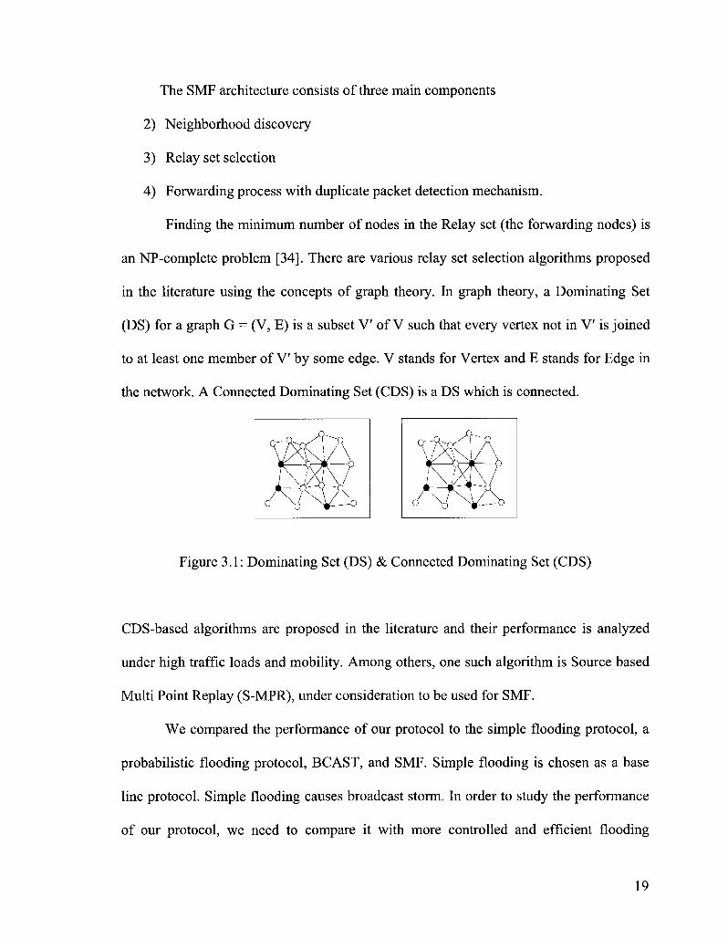
Finding the minimum number of nodes in the Relay set (the forwarding nodes) is
an NP-complete problem [34]. There are various relay set selection algorithms proposed
in the literature using the concepts of graph theory. In graph theory, a Dominating Set
(DS) for a graph G = (V, E) is a subset V of V such that every vertex not in V is joined
to at least one member of V by some edge. V stands for Vertex and E stands for Edge in
the network. A Connected Dominating Set (CDS) is a DS which is connected.
Figure 3.1: Dominating Set (DS) & Connected Dominating Set (CDS)
CDS-based algorithms are proposed in the literature and their performance is analyzed
under high traffic loads and mobility. Among others, one such algorithm is Source based
Multi Point Replay (S-MPR), under consideration to be used for SMF.
We compared the performance of our protocol to the simple flooding protocol, a
probabilistic flooding protocol, BCAST, and SMF. Simple flooding is chosen as a base
line protocol. Simple flooding causes broadcast storm. In order to study the performance
of our protocol, we need to compare it with more controlled and efficient flooding
19
schemes. The second protocol we selected is probabilistic flooding. Probabilistic flooding
is very efficient if the right value of forwarding probability is found and used in the
protocol. However such a protocol is not adaptive as we need to find the best value of
forwarding probability for every changing scenario for best performance. This value, for
example, is very sensitive to the network density. This makes this protocol not practical
for adhoc networks. The next protocol we selected for comparison is BCAST. BCAST is
adaptive and uses neighbour knowledge to decide if the packets need to be forwarded or
not. The PDR and latency performance of this protocol is good for very low data rates of
a few kilobits per second (kbps). Finally we selected SMF, which is considered as one of
the most efficient broadcast protocols developed based on MPR. Hence we compare our
protocol with a wide range of broadcast protocols from baseline flooding to one of the
best, namely, SMF.
3.3 Related Work on RLNC for Wireless Networks
We divided the related work on RLNC for wireless networks in two categories;
Analytical Work and RLNC-based Heuristic Protocols. The details for each category are
provided in the following sections.
3.3.1 Analytical Work
The original work on network coding for multicasting in wireline networks was
done by Ahlswede et al. [3]. They showed that as the symbol size approaches infinity, the
source can multicast information at a rate approaching the min-cut between the source
and any receiver. The work was further extended by Koetter and Medard [36], showing
20
that codes with simple and linear structure were sufficient to achieve capacity in lossless
wireline networks. They presented an algebraic framework for network coding, a
discipline that is already well established in the mathematical world and proved that there
exist coding strategies that provide superior performance without requiring to adapt to the
network interior / structure. They derived their results for both delay-free networks and
networks with delay.
3.3.1.1 NC Performance in Lossless and Lossy Networks
In [37], the authors gave a theoretical overview of network coding in both lossless
and lossy networks for single source unicast & multicast operation. Their theoretical
work shows that, for lossless networks, NC provides no advantage / coding gain in terms
of energy efficiency, robustness and reliability compared to standard routing in case of
unicast traffic. However, for multicast traffic, NC provides considerable gain. For lossy
networks, NC provides coding gain for both unicast as well as multicast traffic. Their
results show the benefit of NC especially in providing robustness and reliability in the
network. The heuristic implementation of the theoretical work provided in their paper
results in a protocol called CodeCast [9], discussed in the next section.
3.3.1.2 NC in Distributed Network Operations
Ho et al. [17] showed that RLNC achieves single source multicast capacity with
probability approaching 1 with the length of the code. They demonstrated their results in
two scenarios - distributed network operation and networks with dynamically varying
connections. They provided a lower bound on the probability of error-free transmission
21
for independent or linearly correlated sources. Another important analysis is that RLNC
effectively compresses arbitrarily correlated sources in the network in a natural way. The
authors compared their distributed NC approach to a Steiner tree routing protocol in their
analysis. The results were compared in terms of blocking probability and throughput.
The results showed that when the connections vary dynamically, NC can offer significant
benefit. Their simulations were based on short network code lengths and networks of 8-
12 nodes. However, the theoretical bound calculated in their work for error-free
transmission is considering large field sizes. It is already shown in [38] that choosing
even a smaller field size of 8 is enough to make the combination dependency negligible.
3.3.1.3 NC Performance in Elastic and Inelastic Networks
The delay performance of RLNC is studied for elastic and inelastic traffic in [6]
for single source broadcast. The authors defined elastic traffic as one with no delay
constraints and inelastic traffic as traffic that has stringent delay constraints. Inelastic
traffic does not enter the system until the minimum delay constraints are guaranteed to be
met. The analytical analysis is done for a single hop system and generalized to multi-hop
networks. The results showed that for elastic traffic there is a significant coding gain
which is proportional of the file size. For inelastic traffic, it is shown that for the same
delay constraints, NC is able to support a larger number of receivers and improve the
throughput of the system. However, in the analysis they assumed Poisson arrival only.
Secondly, in order to extend their work to multi-hop scenarios, they rearranged the
network in layers and assume that there is no communication between nodes in the same
layer for multi-hop networks. Nodes are not allowed to transmit the packets until all the
22

nodes in the same layer have received the packets. They did not mention how the layered
topology will be constructed and the overhead associated with broadcast messages that
will be sent in identifying the layers in which the nodes are to be placed. Finally, their
scheme will not be able to function when there is mobility as the nodes might leave the
layer or enter another layer's region from time to time.
3.3.1.4 NC Comparison with ARQ and FEC Schemes
In [39], the delay performance of network coding for a tree-based single source
multicast problem is studied and compared analytically with various Automatic Repeat
reQuest (ARQ) and Forward Error Correcting (FEC) techniques in terms of effective
number of retransmissions per packet. For network coding, this paper assumes reliable
and instantaneous feedback to acknowledge correct decoding of all data packets. In
practical systems, the acknowledgement can be lost as well, especially in highly
unreliable wireless networks. The work shows the advantage of coding over ARQ in
terms of the expected number of transmissions in a single-path tree or one-hop topology
for lossy networks. NC has been shown to be an efficient reliable wireless multicast
method which achieves a logarithmic reliability gain over ARQ mechanisms. However,
Rateless Coding and link-by-link ARQ achieve comparable performance to that of
network coding. However, their analysis ignores the complexity and overhead associated
with increasing block size. Although they mentioned that their results show that a
reasonable block size is sufficient to obtain the full reliability benefit available via NC,
they did not quantify what they mean by sufficient. The other assumption is that each
23
node of the multicast tree has exactly K children, which is not practical, especially when
we talk about mobile wireless environments.
The reliability performance of RLNC is compared with two different Automatic
Repeat reQuest (ARQ) schemes namely Enhanced ARQ (ARQ-E) and Single Path
Routing ARQ (ARQ-SPR) [26]. Reliability is calculated as the total expected number of
bits transmitted for each information bit transmitted from sender to receiver. Their results
and theoretical analysis show that these advanced ARQ schemes perform comparable to
RLNC. The ARQ-SPR scheme gives comparable performance with negligible overhead.
However, it is observed in their work that the model they have considered is one with a
single sender and a single receiver. We have already discussed that the real benefit of
RLNC is observed in the case of multiple unicasts, multicasting, or broadcasting and the
papers already discussed before acknowledge this fact. The authors have ignored the
coordination and scheduling cost between relay nodes for simplifying the analysis.
However, we have observed from our survey that there is no requirement for such
coordination in the case of RLNC.
3.3.1.5 Energy Efficient Scheme Using NC
Theoretical analysis is provided as well as simple algorithms are proposed for
energy efficient broadcast in [16]. Energy efficiency is directly related to battery life,
which is of significant importance in wireless adhoc as well as sensor networks. Their
work addresses fixed (topologies and link capacities are not changing) as well as
dynamically changing network environments (due to mobility, going to sleep, etc) for all-
to-all communication patterns, which is our interest as well. Their theoretical analysis
24

shows that NC improves performance by a constant factor for fixed networks and by a
log n factor for dynamically changing networks, where n is the number of nodes. Their
assumption in the system model is that a broadcast transmission is successfully received
by all neighbours or the complete transmission will fail. Secondly, each source has only a
single packet to transmit. The paper also described issues related to generation selection
and management based on multi-source scenarios. Although the authors have hinted at
these generation management methods, no detail is provided as to how the generation
management is actually working. Secondly, in their work, they have assumed that each
node has only a single symbol to transmit and all the packets belong to a single
generation. This assumption is not practical in a sense that there will always be multiple
packets to be transmitted by sources and if the number of nodes increases, keeping all the
packets in a single generation will not be practical in terms of memory utilization and
processing time.
3.3.1.6 Improvement of Distributed MAC Protocol using NC
In [25], the authors provided an extension to distributed MAC protocols that
improves efficiency of coding decisions and allows decodability of packets before they
are transmitted. They provided an algorithm (NC-MAC) that manages the stored data
packets intelligently at the MAC queue of each node. The algorithm improves the
knowledge of the node for available correct coding opportunities by using opportunistic
acknowledgements. They showed that their protocol shows significant throughput
improvement compared to standard NC. However this work is related to XOR-based NC,
which works on the neighborhood knowledge of received packets.
25
Similar work is done for the case of unicast traffic [40], showing a 20-30 %
throughput increase using their RLNC-based proposed algorithm, named Multipath Code
Casting (MC2). Another paper shows almost two-fold throughput increase [41] compared
to traditional routing when their RLNC-based algorithm is applied, named Optimized
Multipath Network Coding (OMNC).
3.3.2 RLNC-based Heuristic Protocols
In this section we discuss in detail the various RLNC-based routing algorithms
proposed and their analysis. Later, we sum up the performance of RLNC-based protocols
mentioned in the literature, thus developing the basis for our proposed algorithm.
3.3.2.1 RLNC-based Probabilistic Routing
The first protocol [14] is related to multisource unicast for wireless adhoc
networks using RLNC for probabilistic routing (Delay Tolerant Networking) in extreme
performance-challenging environments. The simulation results show that their proposed
RLNC-based probabilistic routing algorithm achieves high reliability and robustness
compared to a simple probabilistic routing scheme for both static and mobile nodes.
Hashing is performed over the sender address and packet identifier to determine which
generation the packet should belong to. However the paper did not provide much detail
on this hashing operation. In order to forward the packets, a forwarding factor d is
introduced. The results for a static topology show that NC achieves 100% delivery ratio
with less overhead, whereas probabilistic routing results in a three times larger overhead
to achieve the same PDR. For the mobile topology, the authors claim similar results,
26
100% packet delivery ration is achieved with a forwarding factor of 0.125, resulting in 6
times overhead reduction compared to simple probabilistic routing. For sparse networks,
NC performs much better and probabilistic routing almost fails to deliver the packets.
They also investigated the impact of generation size on the overhead and size of matrix.
For a generation size of 4, 99% of PDR is achieved. The results also confirm that an
increase in the generation size improves the network throughput as well as delivery ratio.
However, even a smaller generation size is shown to perform well compared to simple
probabilistic routing.
3.3.2.2 RLNC-based Video Surveillance Protocol
CodeCast [9] is proposed for multimedia applications, especially for surveillance
i.e. for transmitting video images collected from various cameras to the patrolling
security agents in an industrial environment. The main focus is on delay constraints and
delivery ratio for single source wireless multicast. The images should be delivered
successfully within the delay constraints.
The authors used the term "Block" in their research work in lieu of "Generation'''
used in the literature and in our thesis. The application generates equal-sized frames pi ,
p2 ....Adjacent frames are arranged into blocks denoted by (blockid, blocksize). The
blocksize (# of frames to be encoded) is kept variable based on the delay constraints
calculated from the frame generation rate of the application. However their results are
presented for only two distinct block sizes, 4 and 8. The end-to-end delay increases when
the blocksize is increased to 8 as more frames are needed from the application to encode
them. However, increasing blocksize {generation size) improves the network throughput,
27
as also mentioned in other literature. The receiving node has a timer called blocktimeout.
Based on the value of blocktimeout, the node makes the forwarding decision. If all the
packets of a particular block are received, then they are decoded and recovered. However,
as mentioned in [15], some of the packets can be recovered even if fewer than
blocklength packets are received if the rank of the sub matrix is full. However, this paper
did not talk about decoding based on partially received packets. The paper compares the
performance of CodeCast with the On Demand Multicast Routing Protocol (ODMRP),
which is claimed to be one of the best multicast routing protocols in mobile lossy
environments. The results show 100% packet delivery regardless of node speed, block
size and packet drop probability compared to 94% for ODMRP, with less overhead.
3.3.2.3 RLNC-based Broadcast in Realistic Simulation Scenarios
In [15], the authors observed the effect of packet loss and propagation delay using
RLNC. Their work addresses single-source broadcast in wireless adhoc networks. They
showed through simulations that network node density and generation size play an
important role in the performance of RLNC-based broadcast. The encoding, re-encoding
as well as decoding processes are almost similar to that of CodeCast with minute
differences. It is unclear in the paper how the re-encoded packet's rank is identified.
The performance metrics used to evaluate the broadcast schemes are
delay, packet loss rate, protocol overhead and transmission fairness. The results show that
as the network becomes more crowded, NC loses more packets with neighborhood size >
14. The reason given is that, in case of dense networks, there is a higher chance that all
packets are received and the simple broadcast scheme works well. However they did not
28

mention the fact that in case of dense networks, there are more collisions, and packet loss
due to collisions should increase with denser network, thus causing broadcast storm.
Secondly, the results from other references show that in denser networks RLNC shows
better performance. Another important factor is that they have considered only static
scenarios. As described before, much improved performance is achieved for lossy as well
as mobile networks compared to standard broadcast. The protocol overhead for RLNC
decreases when a larger generation size is used, but they did not mention the fact that
once the generation size increases, it affects the delay performance of the algorithm. As
mentioned in previous work, the balance between the delay constraint and generation size
need to be established. Their work lacks this analysis.
3.3.2.4 RLNC-based Broadcast in Dense Environment
Broadcasting with RLNC for dense wireless environment is presented in [42]. The
work is for single-source adhoc networks. In their proposed algorithm, the source node
divides the information into groups of N packets and every packet in the same group is
assigned the same sequence number. If a receiving node finds the sequence number of the
arriving packet to be one that has already been recovered, the node discards that packet.
In simulations, the authors have made the assumption that there is no buffer overflow and
no bit error packet loss. Secondly, decoding failure causes all packets to be lost. They did
not look at the possibility of earlier decoding of packets as mentioned in [15]. The metric
used to judge the performance is decoding failure, packet loss probability vs. node
density, vs. length of coding vector N and vs. order of GF. Their results show that as the
length of the coding vector increases, the number of collided packets decreases.
29

Secondly, as the node density increases, Pioss becomes a convex function. As the number
of nodes increases, there are more chances to successfully decode the packets, but on the
other hand a conflicting situation arises as there are more collisions and the chances of a
decoding failure increases as well. Their Pioss results are also in conflict with the results
mentioned in [15], who showed that RLNC shows poor performance when the number of
nodes increases. Another result between Pioss and length of coding vector shows that there
is strong influence of the size of the coding vector and Pioss- Choosing the optimal vector
size is necessary for better Pioss performance. Similarly, they have shown that the order of
the GF field also has a strong impact on Pioss. The authors did not analyze the
performance of their algorithm in case of mobility and lossy environments.
3.3.2.5 RLNC-based Wireless Broadcast for Multi-player Video Game
Finally, multisource wireless broadcast using RLNC is discussed in [43]. The
algorithm is developed for multi-player video game broadcast for wireless networks
called Network Coded Piggy-Back (NCPB). The proposed algorithm is compared with
IEEE 802.11 broadcast, Piggy-Back Retransmission (PBR) and Multi Point Relay (MPR)
in terms of packet delivery ratio and delay. The simulations were carried out for lossy
static as well as mobile scenarios involving multiple sources. However their work is more
specific to the gaming environment where there is a periodic nature of traffic.
Before starting the game, the N nodes negotiate with each other for entry into and
initialization of the game. Each node obtains an ID and their coding vectors are
exchanged among each other during the initialization phase. Afterwards, each node uses
the same coding vector. The authors did not describe the impact of linearly dependent
30

coding vectors. All the coding vectors generated and exchanged should be checked for
dependency. Another point, as mentioned in [16], is that each source packet should only
be part of one generation but the authors in this paper did not mention anything related to
dealing with this issue or how they are creating generations. The exchanges take place in
each time interval, which are well synchronized between nodes. However, in case of
adhoc networks, an algorithm should be designed that does not require or depend upon
synchronized nodes. This algorithm showed high delivery ratio and less delay suitable for
gaming in all simulations compared to other schemes. Their results also show that once
the node density increases, the performance degrades for other schemes, but the NCPB-
based scheme shows better results. The same performance is observed when conducting
experiments on their test-bed implementation.
3.4 Discussion
As we have seen from the analytical work as well as various proposed protocols
for RLNC, there is a strong potential of using network coding for various applications.
The work on wireless networks shows many promising results. Based on the survey, we
conclude the following for the application of RLNC for wireless applications.
1. RLNC is very suitable for multicast / broadcast applications.
2. The analytical models show the benefit of RLNC in terms of reliability, robustness
throughput and energy efficiency. However, all these models are based on certain
assumption that may limit their analysis in the context of real applications.
3. RLNC shows almost similar performance compared to advanced ARQ and other
controlled flooding schemes in case of static and low density networks. In harsh
31

environments, especially where there is sparse connectivity and lossy links, RLNC
performs better than other counterpart schemes.
4. For dense networks, there are more collisions and hence more retransmissions. RLNC
is shown to provide better results compared to other schemes even though there are
losses due to collisions.
5. In case of mobile networks like MANETs, RLNC performs better and provides more
robustness and reliability with less overhead compared to other schemes
6. The performance of RLNC is very much dependent upon the generation size, size of
GF (symbol size) and how the extra (redundant) transmissions are controlled in case
of broadcasting.
7. Increasing the generation size improves the throughput, but there is a strong relation
between the decoding complexity, delay and selection of a proper generation size.
8. Another important issue is defining the role of intermediate nodes (sub-graph
selection problem). Different papers have proposed various methods to improve the
delivery ratio as well as throughput by storing the coded packets at intermediate
nodes and either decode, partially decode or re-encode the received encoded packets.
An intermediate node also needs to decide whether to send multiple copies or a single
encoded packet.
9. Most schemes have parameters to control the number of retransmissions. However,
these parameters are manually set for each scenario and therefore are not adaptive,
which makes these protocols not suitable for different node densities and speeds. A
suitable algorithm needs to be developed that can take care of all the possibilities and
32

provide the most effective solution for a wide range of dynamically changing
environments.
10. Most of the work in wireless networks is either related to multiple unicast or multicast
scenarios; there is less work done investigating the performance of broadcasting in
adhoc networks using RLNC. There are analytical models as well as a few simulation
papers that discuss broadcast, but there is still a lot of room to develop an algorithm
that is suitable and practical in implementation. Especially very little research has
been done to-date for multi-source broadcast.
11. The problem dealing with multi-source broadcast has to be handled quite differently
from the proposed schemes for a single source. The main issue is how the generation
is to be defined for packets from different sources. Some of the proposals for
selecting a generation include packets generated within a specific area of network,
packets generated over a specific period of time or packets containing a certain type
of information.
12. It is mentioned in the literature [42] that for multi-source broadcast, the initial
assumption is that all the nodes are well synchronized. However our protocol is
totally distributed in nature and does not require node synchronization.
13. To the best of our knowledge, there has been no comparison of the performance of
multi-source wireless broadcast with and without cross-session generations in the
literature. The cross-session generation concept is explained in more detail in the next
chapter.
33

Chapter 4
Proposed Model
4.1 Adaptive Random Linear Network Coding with Controlled
Forwarding (ARLNCCF)
Based on the analysis from Chapter 3, we propose Adaptive Random Linear
Network Coding with Controlled Forwarding (ARLNCCF) for broadcasting in wireless
adhoc networks. The proposed algorithm is carefully designed based on the concepts and
shortcomings of previously proposed algorithms. Our main target is to present a single
algorithm that can meet the needs of various environments and situations and is not
limited to a single scenario, hence the reason we call our protocol adaptive. This chapter
introduces our approach and our algorithm's functionality in detail.
4.2 Proposed Scheme
RLNC is highly distributed in nature. Unlike XOR-based or Reed-Solomon-based
coding, which require the knowledge of what its neighbours have received to encode the
packets, no such information is required by RLNC. Broadcasting is an important
communication technique and needs the same attention as unicast and multicast. Most of
the work found in the literature is addressing the case of single source broadcasting.
There are few proposed adaptive algorithm dealing with multi-source broadcasting. Our
algorithm will be suitable for both single source and multi-source broadcasting. It is
observed from the previous work that RLNC works well for dense, mobile and lossy
34

environments where other algorithms show poor performance [42]. However, if the node
density is small, its performance depends upon how many packets are encoded together
to obtain a better coding gain [14]. ARLNCCF is able to combine packets from the same
source or multiple sources based on available generations and their sizes in the buffer.
Our protocol follows the basic idea of RLNC as discussed in Chapter 2. We got
the inspiration from [9][15] [16] to develop our protocol. It is mentioned in the literature
[38][44] that GF(28) is sufficient for the symbol size to maintain linear independence with
high probability. So for simplicity and byte-by-byte operation, we set the symbol size to 8
in our implementation. Some of the terms used are as following,
Coded packet
Once the source generates the packet, it is encoded with a random coefficient from
GF(28), the resultant packet is called coded packet. This packet is re-encoded with other
coded packets in the generation (if they exist) before transmission.
Re-encoded packet
When the existing coded packets are further encoded with random coefficients from
GF(2 ), the resultant packet is called a re-encoded packet.
Decoding matrix
All the packets are stored locally in generations in the form of a decoding matrix. Each
row of the matrix contains the coefficients of the coded/re-encoded packet.
Coded vector
The vector of coefficients that are stored as rows in the decoding-matrix for each
encoded/re-encoded packet is called coded vector for that packet.
35
Cross-session generations
Generations that are not confined to particular sources (generations having
symbols from the same source only) and allow inter-mixing of symbols from different
sources are called cross-session generations. In this thesis we show that cross-session
generations improve PDR and reduce latency compared to generations that do not allow
symbols to be combined from different sources (see results in Section 7.1)
The unique features of our protocol that make it adaptive and support cross-
session design are discussed in the following sections.
4.2.1 Hello Control Messages and Number of Retransmissions
In order to adapt the number of retransmissions as well as the probability of
broadcast, we need to maintain the neighborhood information for the topology. Based on
this neighborhood information, the algorithm can decide about the node density as well as
the number of retransmissions required.
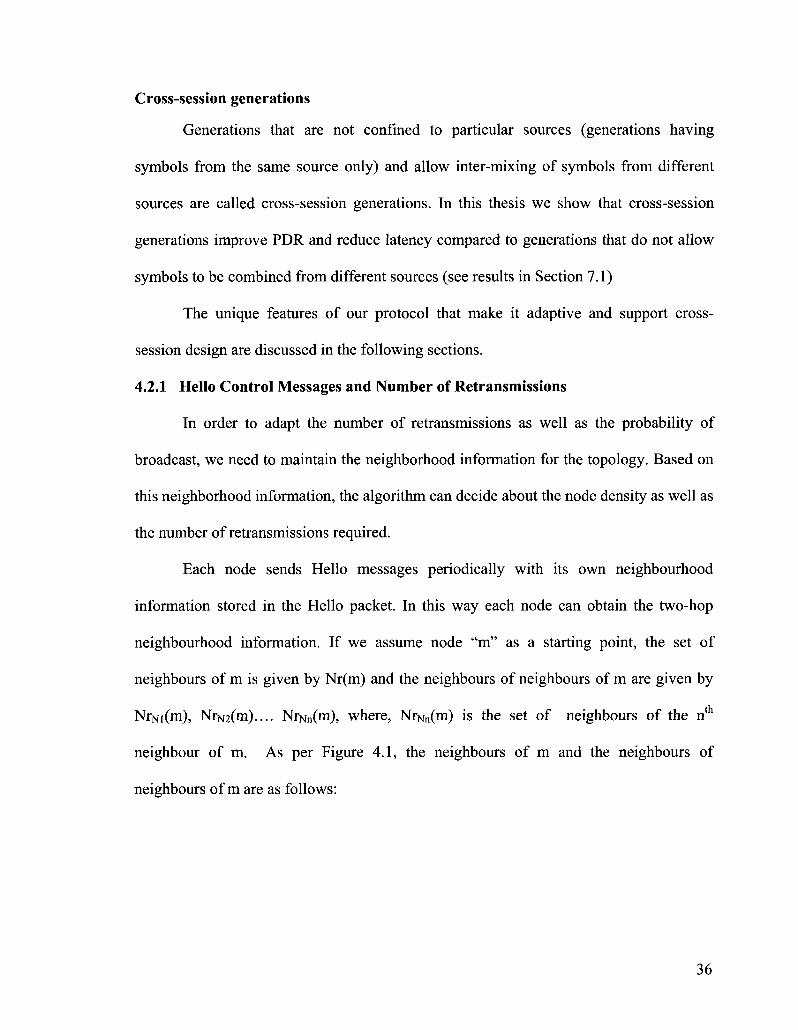
Each node sends Hello messages periodically with its own neighbourhood
information stored in the Hello packet. In this way each node can obtain the two-hop
neighbourhood information. If we assume node "m" as a starting point, the set of
neighbours of m is given by Nr(m) and the neighbours of neighbours of m are given by
NrNi(m), NrN2(m).... NrNn(m), where, NrNn(m) is the set of neighbours of the nth
neighbour of m. As per Figure 4.1, the neighbours of m and the neighbours of
neighbours of m are as follows:
36
/"'" d4 "\
-•• •. 1 ~. .~-0m <T)N ' i
Figure 4.1: Neighborhood of Node m
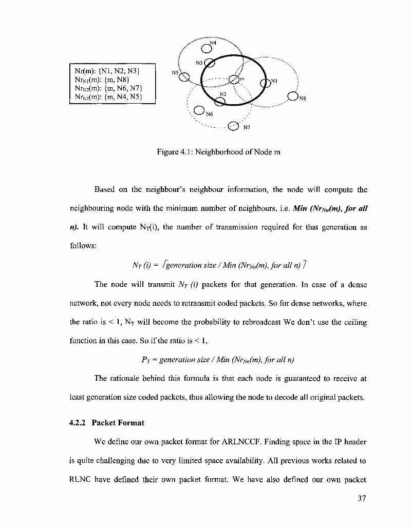
Based on the neighbour's neighbour information, the node will compute the
neighbouring node with the minimum number of neighbours, i.e. Min (NrNn(m), for all
n). It will compute Nx(i), the number of transmission required for that generation as
follows:
NT (i) = I generation size / Min (Nr^„(m), for all n) /
The node will transmit Nj (i) packets for that generation. In case of a dense
network, not every node needs to retransmit coded packets. So for dense networks, where
the ratio is < 1, NT will become the probability to rebroadcast We don't use the ceiling
function in this case. So if the ratio is < 1,
Pj = generation size / Min (NrNn(m),for all n)
The rationale behind this formula is that each node is guaranteed to receive at
least generation size coded packets, thus allowing the node to decode all original packets.
4.2.2 Packet Format
We define our own packet format for ARLNCCF. Finding space in the IP header
is quite challenging due to very limited space availability. All previous works related to
RLNC have defined their own packet format. We have also defined our own packet
37
Nr(m): {NI, NrN1(m): NrN2(m): NrN3(m):
{m {m {m
N2, N3} N8} N6 N4
N7} N5}

header format where the required information will be stored. In the header, each coded
symbol needs to be identified in the encoded vector attached to the packet. We identify
each symbol with a Sequence Number (16 bit) and IP address (32 bit) pair. The header
fields are shown in Figure 4.2.
0 15 16 23 24 31
Generation ID Generation Distance Length
IP address and Sequence Number pair
(32 bit IP address & 16 bit sequence number)
IP address and Sequence Number pair
(32 bit IP address & 16 bit sequence number)
Encoding/Re-encoding Coefficients (8 bits per coefficient)
payload
Figure 4.2: Packet Format for ARLNCCF
The Generation ID is the 16 bit number used to represent each generation
uniquely at the given period of time. Generation Distance is an 8 bit number and is
explained in detail in Section 4.2.5. The length field specifies how many source address
and sequence number pairs we have. The IP address and Sequence Number pair is used to
uniquely identify the original packet in the encoded vector. We have as many pairs as that
of number of original packets encoded together. This pair is required because if we just
38

use one parameter than there is no way to distinguish packets from one source to another.
Each source maintains its own sequence number and each packet can only be
distinguished by its sequence number and the source address generating that sequence
number. Similarly, we have as many coding/ re-encoding coefficients (encoding vector)
as that of source address and sequence number pairs. This encoding vector is inserted in
the respective Generation as the last row in the decoding matrix by the receiving node.
Finally we have the payload part which contains the actual coded packet.
In order to implement our protocol in real world, we need a new protocol value in
the IP header's "Protocol" field. This value is assigned by the Internet Assigned Numbers
Authority (IANA). An ARLNCCF packet is carried as the payload of an IP packet. At
layer 3, once the IP header's protocol field is examined with our protocol value, the
packet will be send to the ARLNCCF protocol implementation for further processing.
4.2.3 Generation Size
Since our main aim is to develop a multi-source protocol and nodes are free to
insert their packets in any generation, there will always be cases where different nodes
insert their symbols in the same slot of a given generation based on their local space in
that generation. The receiving node maintains an ordered list of source addresses and
sequence numbers for each locally saved generation. Once a coded packet arrives, the
node reorders the symbols of the receiving packet based on its local ordered list. If a
symbol is found with a different 2-tuple for the same slot, this symbol is moved to the
available space in that generation. If no space is available, the generation size is increased
by 1 and the conflicting symbol is added to the end.
39

4.2.4 Generation Timeout
Motivated by the generation timer concept introduced in [9][15], our protocol also
has a timer T associated with each generation. The required number of encoded packets is
rebroadcasted after the timer expires. However, there is still a chance that the node
receives more innovative packets after T has expired. In that case, a single packet is
rebroadcast for each received innovative packet if NT> 1.
4.2.5 Generation Distance (GD)
In order to control the generation size and to avoid increasing it by a large value,
especially at high data rates and a large number of senders, we introduce the idea of a
generation distance. It works as follows:
1. The source, creating the new generation, sets the generation distance to 0 for that
generation. The rebroadcasted packets for that generation have this value set to 1 in
the packet header.
2. When the node receives a packet, it compares the generation distance value for that
generation with the value in the packet. If the packet value is less than the locally
stored value, the locally saved value is replaced with the packet value. In this way the
minimum hop distance is known to the node from where the generation was created.
3. If the source inserts its packet in another generation, not created locally, the value
remains unchanged and the re-encoded packet for that generation has the value
incremented by 1.
4. To insert a new packet, locally created generations are preferred. If none are
available, then the generation with minimum GD is preferred, as long as the GD value
40
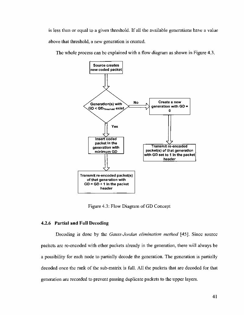
is less than or equal to a given threshold. If all the available generations have a value
above that threshold, a new generation is created.
The whole process can be explained with a flow diagram as shown in Figure 4.3.
Source creates new coded packet
Yes
iz Insert coded packet in the
generation with minimum GD
iz
No -N
Create a new generation with GD :
0
XZ Transmit re-encoded
packet(s) of that generation with GD set to 1 in the packet
header
Transmit re-encoded packet(s) of that generation with
GD = GD + 1 in the packet header
Figure 4.3: Flow Diagram of GD Concept
4.2.6 Partial and Full Decoding
Decoding is done by the Gauss-Jordan elimination method [45]. Since source
packets are re-encoded with other packets already in the generation, there will always be
a possibility for each node to partially decode the generation. The generation is partially
decoded once the rank of the sub-matrix is full. All the packets that are decoded for that
generation are recorded to prevent passing duplicate packets to the upper layers.
41
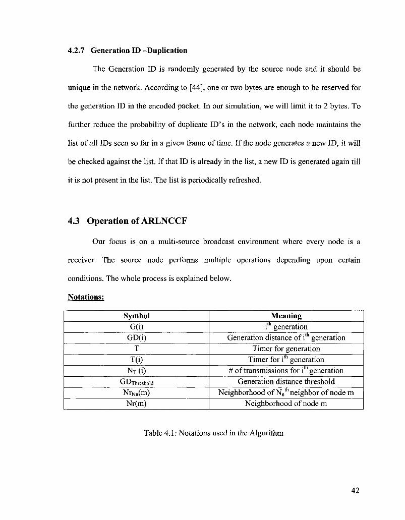
4.2.7 Generation ID -Duplication
The Generation ID is randomly generated by the source node and it should be
unique in the network. According to [44], one or two bytes are enough to be reserved for
the generation ID in the encoded packet. In our simulation, we will limit it to 2 bytes. To
further reduce the probability of duplicate ID's in the network, each node maintains the
list of all IDs seen so far in a given frame of time. If the node generates a new ID, it will
be checked against the list. If that ID is already in the list, a new ID is generated again till
it is not present in the list. The list is periodically refreshed.
4.3 Operation of ARLNCCF
Our focus is on a multi-source broadcast environment where every node is a
receiver. The source node performs multiple operations depending upon certain
conditions. The whole process is explained below.
Notations:
Symbol G(i)
GD(i) T
T(i)
NT(i) GDihreshold
NrNn(m) Nr(m)
Meaning ith generation
Generation distance of ith generation Timer for generation
Timer for ith generation # of transmissions for ith generation
Generation distance threshold Neighborhood of Nn
th neighbor of node m Neighborhood of node m
Table 4.1: Notations used in the Algorithm
42

4.3.1 Source Node Operation
1. The source generates a packet. The packet consists of multiple symbols of 8 bit each.
If we assume an IP packet length of 1400 bytes, there will be (up to) 1400 symbols in
each packet, considering GF (28). The encoding operation is performed on each
packet.
2. Once the packet is generated, the node checks if there are already some generations
available in the memory with GD < GD-rhreshoid-
Source generates
symbols of packets
No
0. Create new generation with random ID. Encode the packet and create coded vector.
zs
Find the generation G(i) with lowest generation distance
(S(i) < Smax) If locally created generation exists, it is preferred as its
generation distance is 0
No
• Encode the packet and insert in G(i).
• Re-encode all the packets in that generation.
•r
Initialize the decoding matrix and add encoded vector to this generation. Start the timer T
-N
1Z Create the packet with required format. Transmit single packet = >
Figure 4.4: Flow Diagram - Encoding Process
43

3. If YES (Generations exist in the memory):
a. Find the generation G(i) in memory with lowest generation distance, i.e. min
GD(i). If there are more than one generations with same minimum GD value,
than the first generation found by the algorithm with that GD value is used.
b. Generate a random coefficient from GF(28) for that packet and insert the
packet in the generation G(i).
c. Re-encode all the available coded vectors including the source vector in the
decoding matrix. A single coded packet is broadcasted.
4. If NO (No suitable generation is available in memory):
a. A new generation is created with randomly selected generation ID. The
generation is saved in the memory in the form of a decoding matrix.
b. The coded vector is created by choosing random coding coefficients.
c. An encoded packet is created with the header containing the generation ID
and coding coefficients.
d. A single encoded packet is broadcasted, as this generation contains one new
source packet.
Example: Source packet insertion
Source SI has a packet m4 to send. The packet is encoded with random
coefficient, \K3 = g5 * m4\, where g5 is taken from GF (2 ). If no generation is available
then a new generation is created and x3 is inserted in the new generation and transmitted
(there is no re-encoding in this case). We assume that the source already has two coded
packets in the some generation in the memory, ]gl * ml+ g2 * m2\ and g3 * ml + g4
m3\. The two coded packets contain symbols from 3 original packets, ml, m2 and m3.
44
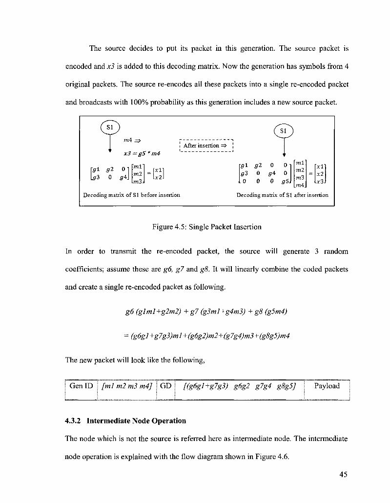
The source decides to put its packet in this generation. The source packet is
encoded and x3 is added to this decoding matrix. Now the generation has symbols from 4
original packets. The source re-encodes all these packets into a single re-encoded packet
and broadcasts with 100% probability as this generation includes a new source packet.
® m4 .
® x3 = g5 * m4
i After insertion => ] i i
[51 g2 en Us 0 54J
m l ml ni3.
\xl] 1x21
Decoding matrix of SI before insertion
m l m2 m3 .m4.
Decoding matrix of SI after insertion
g\ g2 0 0- | 5 3 0 g4 0 . 0 0 0 # 5
aril x2
1x31
Figure 4.5: Single Packet Insertion
In order to transmit the re-encoded packet, the source will generate 3 random
coefficients; assume these are g6, g7 and g8. It will linearly combine the coded packets
and create a single re-encoded packet as following.
g6 (glml+g2m2) + g7 (g3ml+g4m3) + g8 (g5m4)
= (g6gl +g7g3)ml+(g6g2)m2+(g7g4)m3+(g8g5)m4
The new packet will look like the following,
Gen ID i [ml m2 m3 m4] \GD\ f(g6gl+g7g3) g6g2 g7g4 g8g5J Payload
4.3.2 Intermediate Node Operation
The node which is not the source is referred here as intermediate node. The intermediate
node operation is explained with the flow diagram shown in Figure 4.6.
45
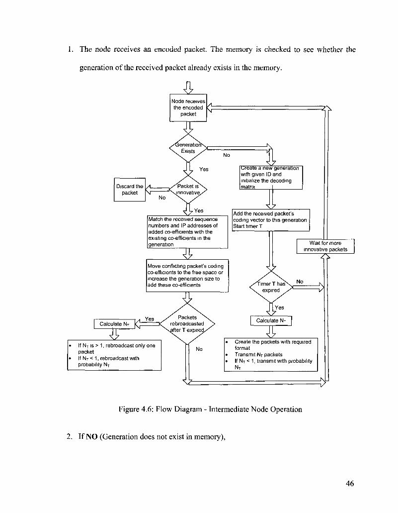
1. The node receives an encoded packet. The memory is checked to see whether the
generation of the received packet already exists in the memory.
ives A
=2T% Node receives the encoded
packet v
Discard the packet
A-
No
iz (Jreate a new generation with given ID and initialize the decoding matrix
Match the received sequence numbers and IP addresses of added co-efficients with the existing co-efficients in the generation
IE
Iz Add the received packet's coding vector to this generation Start timer T
Move conflicting packet's coding co-efficients to the free space or increase the generation size to add these co-efficients
Calculate NT ^
3E If NT is > 1, rebroadcast only one packet If NT < 1, rebroadcast with probability NT
Wait for more innovative packets
z^
£
Calculate NT
A Create the packets with required format Transmit NT packets If NT < 1, transmit with probability NT
V
Figure 4.6: Flow Diagram - Intermediate Node Operation
2. If NO (Generation does not exist in memory),
46
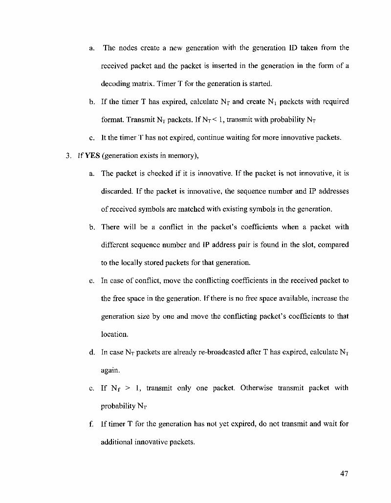
a. The nodes create a new generation with the generation ID taken from the
received packet and the packet is inserted in the generation in the form of a
decoding matrix. Timer T for the generation is started.
b. If the timer T has expired, calculate NT and create NT packets with required
format. Transmit NT packets. If NT< 1, transmit with probability NT
c. It the timer T has not expired, continue waiting for more innovative packets.
3. If YES (generation exists in memory),
a. The packet is checked if it is innovative. If the packet is not innovative, it is
discarded. If the packet is innovative, the sequence number and IP addresses
of received symbols are matched with existing symbols in the generation.
b. There will be a conflict in the packet's coefficients when a packet with
different sequence number and IP address pair is found in the slot, compared
to the locally stored packets for that generation.
c. In case of conflict, move the conflicting coefficients in the received packet to
the free space in the generation. If there is no free space available, increase the
generation size by one and move the conflicting packet's coefficients to that
location.
d. In case NT packets are already re-broadcasted after T has expired, calculate NT
again.
e. If NT > 1, transmit only one packet. Otherwise transmit packet with
probability NT
f. If timer T for the generation has not yet expired, do not transmit and wait for
additional innovative packets.
47
Example: Conflicting Packets (Free Slot Available)
In order to explain how the conflicting packets are resolved, we consider the
following example. We assume that the generation size is 4. Each packet is divided into
equal sized symbols of 8 bits each. Suppose that a locally saved generation with
generation ID 73098 has the decoding matrix given in Figure 4.7.
Gen ID 73098
Source address
Sequence Number
SlotO
1
1
Slotl
2
3
Slot 2
3
6
Slot 3
0
0
36
48
109
0
42
62
154
0
50
64
80
0
0
0
0
0
Figure 4.7: Generation with Symbol Location and Respective Coding Coefficients
The generation has 3 vectors stored locally. (1,1), (2,3) and (3,6) represent the 2-
tuple (source address, sequence number) for each saved packet with their coefficients at
slot 0,1 and 2 respectively. Slot 3 is empty.
We assume that the node with the above generation matrix received a packet for
that generation with the coefficients and address / sequence number pair as given in
Figure 4.8.
48

Gen ID 73098
Source address
Sequence Number
SlotO
1
1
Slotl
2
4
Slot 2
3
6
Slot 3
2
3
66 184 22 170
Figure 4.8: Received Packet with Symbol Location and Respective Coefficients
The received packet has the 2-tuple (2,4) at slot 1. However the locally saved
generation has the coefficients for packet with 2-tuple (2,3) at slot 1. This conflict is
resolved by moving the conflicting coefficients to slot 3 of the generation, which is free.
Similarly, the 2-tuple (2,3) in the received packet in slot 4 is moved to slot 1 of the
locally saved generation. In this way, each node maintains a conflict-free generation.
Gen ID 73098
Source address
Sequence Number
SlotO
1
1
Slotl
2
3
Slot 2
3
6
Slot 3
4
2
36
48
109
66
42
62
154
170
50
64
80
22
0
0
0
184
Figure 4.9: Generation 73098 after Conflict Resolution
It should also be noted that due to this shuffle of coefficients, each node maintains
the order of coefficients independent of other nodes and this order has local meaning
only. Similarly, once the coefficients are moved to a particular slot, the respective coded
49

symbols for that packet are also moved accordingly. After resolving the conflict, the new
generation entries are given in Figure 4.9.
Example: Conflicting Symbols (No Free Slot Available)
In order to explain how the conflicting packets are resolved in case where no free
slot is available in the generation, we consider the following example. We assume that
the generation size is 4. Suppose that the locally saved generation with generation ID
73098 has the decoding matrix given in Figure 4.10. The generation has 3 vectors stored
locally. (1,1), (2,3), (3,6) and (4,2) represent the 2-tuple (source address, sequence
number) for each saved packet with their coefficients at slot 0, 1,2, and 3 respectively.
Gen ID 73098
Source address
Sequence Number
SlotO
1
1
Slotl
2
3
Slot 2
3
6
Slot 3
4
2
36
48
109
0
42
62
154
0
50
64
80
0
69
102
09
0
Figure 4.10: Generation 73098 with Symbol Location and Respective Symbols
We assume that the node with the above generation matrix received a packet for
that generation with the coefficients and address / sequence number pair as given in
Figure 4.11.
50
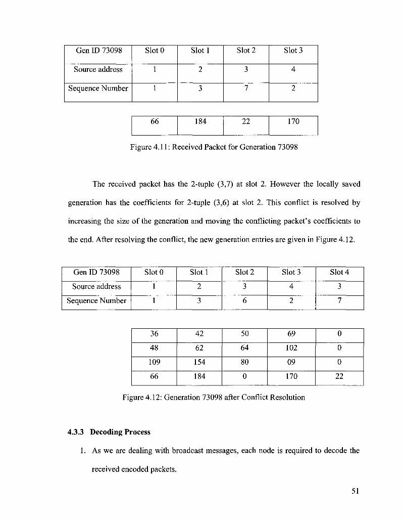
Gen ID 73098
Source address
Sequence Number
SlotO
1
1
Slotl
2
3
Slot 2
3
7
Slot 3
4
2
66 184 22 170
Figure 4.11: Received Packet for Generation 73098
The received packet has the 2-tuple (3,7) at slot 2. However the locally saved
generation has the coefficients for 2-tuple (3,6) at slot 2. This conflict is resolved by
increasing the size of the generation and moving the conflicting packet's coefficients to
the end. After resolving the conflict, the new generation entries are given in Figure 4.12.
Gen ID 73098
Source address
Sequence Number
SlotO
1
1
Slotl
2
3
Slot 2
3
6
Slot 3
4
2
Slot 4
3
7
36
48
109
66
42
62
154
184
50
64
80
0
69
102
09
170
0
0
0
22
Figure 4.12: Generation 73098 after Conflict Resolution
4.3.3 Decoding Process
1. As we are dealing with broadcast messages, each node is required to decode the
received encoded packets.
51

2. Upon receiving an innovative packet, add the received packet to the last row of
the decoding matrix.
3. If the rank is full, decode all the packets.
4. If the rank is not full, try to partially decode the matrix (i.e., check if the rank of a
sub-matrix is full). If some packets are successfully decoded, send the decoded
packets to the upper layer.
5. All 2-tuples for decoded packets are kept in a separate list for that generation. By
doing so we make sure that the same packets are not sent to the upper layer again
once the generation is partially or fully decoded again later.
Innovative packet has arrived
Iz Add innovative packet as last row in the respective
decoding matrix
Decode all the packets and give to upper layer which are not already
decoded
\ 7
Partially decode the matrix, keep the decoded packets in the buffer to avoid duplicate decoding. Deliver the decoded packets to upper layer which are not already decoded for that generation
Figure 4.13: Flow Diagram - Decoding Process
52

• Early Decoding Example
As mentioned before, we get a chance to decode the symbols without waiting for
the generation to reach full rank. We get the chance to early decode the generations when
a sub-matrix rank is full. Some of the examples illustrating the situations where a sub-
matrix has full rank are given in Figure 4.14. The boxes indicate the sub-matrix with full
rank.
48 23 34 23
112 44 54 0
212 108 0 0
231 0 0 0
30 0 0 oJ
[23 34 i23
44 54 87
1081 0 0 J
23 34 13 )0
44 54 105 45
108 212 98 20
75 0 0 0
12' 0 0 oJ
23 44 108 89 34 54 16 0 23 0 0 0
23 44 108 199 34 54 65 15 23 11 0 0
No chance
23 44 108 75 12 34 54 212 30 0
0 0 0 0 0 0
23 105 L90 45
Figure 4.14: Early Decoding Examples
Early decoding has a major impact on reducing the end-to-end packet delay. Even
if, by chance, the decoding matrix never reaches full rank due to the loss of packets, we
can still decode some packets rather than losing all the packets of that generation.
Similarly, if some packets have been received and we get the chance of early decoding,
these packets do not have to wait for the generation to become full, which reduces the
packet latency. However, early decoding can result in out-of-order decoding (and
delivery to the higher layers) of packets. If the node is able to decode sequence number 4
53

before sequence number 3 for some node, then the packets need to be reordered by the
transport layer.
54
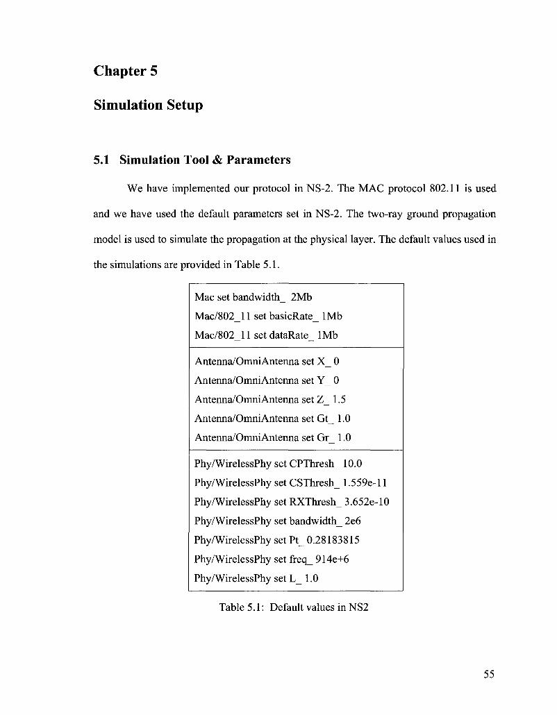
Chapter 5
Simulation Setup
5.1 Simulation Tool & Parameters
We have implemented our protocol in NS-2. The MAC protocol 802.11 is used
and we have used the default parameters set in NS-2. The two-ray ground propagation
model is used to simulate the propagation at the physical layer. The default values used in
the simulations are provided in Table 5.1.
Mac set bandwidth_ 2Mb
Mac/80211 set basicRate_ 1Mb
Mac/802 11 set dataRate 1Mb
Antenna/OmniAntenna set X_ 0
Antenna/OmniAntenna set Y_ 0
Antenna/OmniAntenna set Z_ 1.5
Antenna/OmniAntenna set Gt 1.0
Antenna/OmniAntenna set Gr 1.0
Phy/WirelessPhy set CPThresh_ 10.0
Phy/WirelessPhy set CSThresh_ 1.559e-l 1
Phy/WirelessPhy set RXThresh_ 3.652e-10
Phy/WirelessPhy set bandwidth_ 2e6
Phy/WirelessPhy set Pt_ 0.28183815
Phy/WirelessPhy set freq_ 914e+6
Phy/WirelessPhy set L_ 1.0
Table 5.1: Default values in NS2
55

The default parameters specify that the total bandwidth is set to 2 Mbps where the
rate for data frames is 1 Mbps and rate for control frames is also 1 Mbps. Omni
directional antenna is used by each mobile node and the antenna height is specified by
Antenna/OmniAntenna set Z 1.5. Transmit and receive antenna gain is set to 1.
CPThresh_ , CSThresh_ and RXThresh_ are important parameters and specify the
collision threshold, carrier sense power and receive power threshold. The default values
specify the maximum node reception range to be 250 meters. Since we are using Omni
directional antenna, the node reception range forms a circle of 250 meter radius around
the node. However the interference range / carrier sense range is 550m.
5.2 Performance Metrics
We ran each simulation for 500 second simulation time and averaged over 10
different runs. The performance metrics used to evaluate our algorithm are as following.
PDR
Packet Delivery Ration (PDR) is the ratio of the total number of packets actually
received by each node relative to the total number of packets that should be received
ideally. Ideally, in case of broadcasting, all packets sent by each source should be
received by all the nodes (including the sources) in the network. In case of network
coding, only those packets are considered that are successfully decoded by each node.
Merely receiving the packet does not mean that the received packet is meaningful, unless
it is decoded successfully. The PDR is calculated as following
PDR = (Total packets received by each node) / (Totalpackets sent by each source x
number of nodes)
56

End-to-end packet delay / latency
End-to-end packet latency is the total time between sending a packet at the source
and its successful reception at the receiver. In case of network coding it is the time
between sending a coded packet at the source and its successful decoding at the receiver.
For broadcasting, there are different ways to calculate the packet latency as all the nodes
are receivers. We can calculate it in 3 different ways.
1) Maximum latency: For each packet transmitted, it is the maximum time it takes to
receive that packet by any node. Ideally, nodes that are furthest from the source in
terms of number of hops should have maximum latency. We calculate the
maximum latency for each transmitted packet and then average it over the total
number of packets sent by all the sources.
2) Minimum latency: For each packet transmitted, it is the minimum time it takes to
receive that packet by any node provided that the node is not the source. If we
include the source, minimum latency will always be 0. We calculate the minimum
latency for each transmitted packet and then average it over total number of
packets sent by all the sources.
3) Overall average latency: To calculate the overall average latency, we first
calculate the average of all the times for single packet sent and received by all the
nodes in the network. The calculated average for each packet is again averaged
over all the packets transmitted by all the sources.
In this thesis we used the overall average latency for comparisons. Average
latency is a good measure of overall system latency and we deal with one parameter only
rather than 2 parameters (Minimum & Maximum) for latency.
57

MAC transmissions
We further evaluate the performance of our protocol in terms of the total number
of packet transmissions at the MAC layer. It includes both the data packets and control
packets to justify the comparison with other protocols. Ideally, a given protocol will
achieve high PDR and low latency with a low number of packet transmissions at the
MAC layer, indicating low overheads and efficient use of the wireless media.
5.3 Algorithms for Comparison
We choose simple flooding, probabilistic flooding, BCAST and SMF for
comparing the performance of our protocol using the above mentioned metrics.
1) For simple flooding, the packet is forwarded as soon as it reaches the node's
network layer. Duplicate packets are discarded.
2) For probabilistic flooding, each node retransmits the received packets with
probability P. This significantly reduces the broadcast storm problem of simple
flooding. It is very important that the right value of probability of retransmission
is used that gives the optimal performance. For our scenarios, we found the
following optimal values for different node densities and data rates. For each data
point we need to find this optimal value as given in Table 5.2.
3) BCAST [30], which is based on the Neighbour Knowledge Method, exchanges
periodic HELLO messages to collect 2-hop neighbourhood information. For
retransmission, the receiving node A reschedules the packet with random delay if
all the neighbours of A are not covered by the previous hop B of the received
packet. If the same packet arrives from another neighbour (or set of neighbours) C
58

who covers the remaining neighbours, A discards the packet. The delay is
calculated by multiplying the uniformly distributed randomly generated number
by the ratio of the highest number of neighbours of neighbours of A divided by
total number of neighbours of A and the scaling factor for BCAST.
Static Scenarios
01 - Source
Rate
1
50
100
P value
0.5
0.25
0.15
04 - Source
Rate
1
25
50
P Value
0.4
0.20
0.15
01 - Source
Nodes
05
25
50
75
100
P Value
0.6
0.5
0.25
0.2
0.1
04 - Source
Nodes
25
50
75
100
P Value
0.3
0.15
0.1
0.1
Mobile Scenarios
01 - Source
Rate
1
50
100
P value
0.45
0.20
0.1
04 - Source
Rate
1
25
50
P Value
0.3
0.1
0.1
01 - Source
Nodes
05
25
50
75
100
P Value
0.6
0.5
0.25
0.2
0.1
04 - Source
Nodes
25
50
75
100
P Value
0.25
0.15
0.1
0.1
Table 5.2: Optimal P values used for Probabilistic Flooding
59
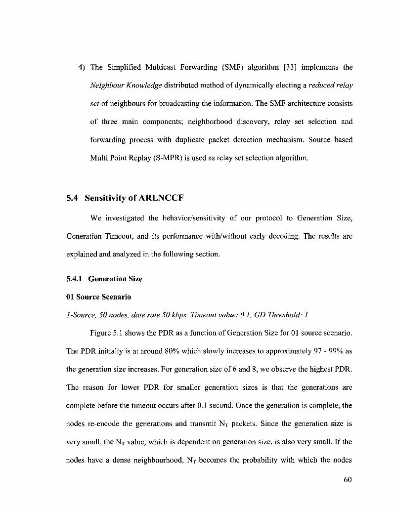
4) The Simplified Multicast Forwarding (SMF) algorithm [33] implements the
Neighbour Knowledge distributed method of dynamically electing a reduced relay
set of neighbours for broadcasting the information. The SMF architecture consists
of three main components; neighborhood discovery, relay set selection and
forwarding process with duplicate packet detection mechanism. Source based
Multi Point Replay (S-MPR) is used as relay set selection algorithm.
5.4 Sensitivity of ARLNCCF
We investigated the behavior/sensitivity of our protocol to Generation Size,
Generation Timeout, and its performance with/without early decoding. The results are
explained and analyzed in the following section.
5.4.1 Generation Size
01 Source Scenario
1-Source, 50 nodes, date rate 50 kbps. Timeout value: 0.1, GD Threshold: 1
Figure 5.1 shows the PDR as a function of Generation Size for 01 source scenario.
The PDR initially is at around 80% which slowly increases to approximately 97 - 99% as
the generation size increases. For generation size of 6 and 8, we observe the highest PDR.
The reason for lower PDR for smaller generation sizes is that the generations are
complete before the timeout occurs after 0.1 second. Once the generation is complete, the
nodes re-encode the generations and transmit NT packets. Since the generation size is
very small, the NT value, which is dependent on generation size, is also very small. If the
nodes have a dense neighbourhood, NT becomes the probability with which the nodes
60

transmit. Nodes re-encode and transmit the encoded packets with very small probability
of retransmission. As a result, some of the nodes never get a chance to completely decode
the generation. Similarly, after the re-encoding operation, with smaller generation sizes,
the chances of receiving more innovative packets is also very much reduced. As the
generation size further increases to 6 and above the PDR improves. The latency is more
or less constant as the generation size increases as shown in Figure 5.2. The reason for
this is that we are doing early decoding and most of the packets get the chance to be
decoded early.
In this research work, since we are more focused on multi-source scenarios, we
have done more investigation of the sensitivity of the protocol for multi-source scenarios.
PDR vs. Generation Size
6 7 8 9 Generation Size
10 11 12
Figure 5.1: PDR vs. Generation Size (01 Source)
61
LATvs Generation Size
o
1
09
08
07
06
05
04
03
0 2
01
0
~i r
7 8 Generation Size
- •— ARLNCCF
10 11 12
Figure 5.2: Latency vs. Generation Size (01 Source)
04 Source Scenarios
4-Source, 50 nodes, date rate 25kbps per source. Timeout value: 0.1, GD Threshold: 1
Figure 5.3 shows PDR as a function of Generation Size. It is observed that the
PDR is around 80% for a very small generation size and it increases to around 96% for a
generation size 4. PDR starts to decline again as the generation size increases. For a
timeout value of 0.1 seconds, a generation size of 4 gives the best performance in terms
of PDR.
62
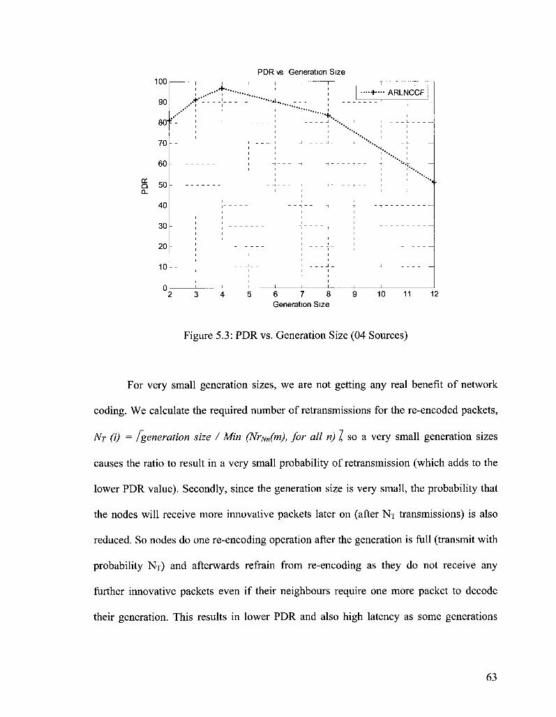
PDR vs Generation Size 100
90
80 f
70
60
01 en Q 50 Q.
40
30
20
10
0
i i
1 . . . • • * • • • • • •+-••• ARLNCCF
i i '"••+.
. j * i . i
6 7 8 Generation Size
10 11 12
Figure 5.3: PDR vs. Generation Size (04 Sources)
For very small generation sizes, we are not getting any real benefit of network
coding. We calculate the required number of retransmissions for the re-encoded packets,
NT (i) = Fgeneration size / Min (NrN„(m), for all n) J so a very small generation sizes
causes the ratio to result in a very small probability of retransmission (which adds to the
lower PDR value). Secondly, since the generation size is very small, the probability that
the nodes will receive more innovative packets later on (after NT transmissions) is also
reduced. So nodes do one re-encoding operation after the generation is full (transmit with
probability NT) and afterwards refrain from re-encoding as they do not receive any
further innovative packets even if their neighbours require one more packet to decode
their generation. This results in lower PDR and also high latency as some generations
63

wait longer to receive the innovative packets from any neighbouring node to decode the
generation fully. Figure 5.4 shows latency as a function of Generation Size.
Mathematically, if a node received ax+by = c, it has to wait for another innovative
packet to solve the equation. For very small generation sizes, this probability (to receive
more innovative packets) is reduced. Even with early decoding, we cannot decode the
packets from a single equation with 2 unknowns and need to wait for another innovative
packet. Overall, a very small generation size causes fewer MAC transmissions but causes
higher latency and lower PDR.
Latency vs Generation Size 1
09
08
07
06
§ 05 CD
- J
04
03
02
0 1
0
i i i
, i
i i
1 '
1
i
^ , ! -
_ _ _ +" ! -- -
i i i
i i
J
-1 4
H H -
t
~I
J
1 1
1 i i
— • — ARLNCCF
! 1 1 L
, ,__ , . _
_ + 1 ^
-t- -f t-
; - - - r
_ _
' - - -
i
3 4 5 6 7 8 9 10 11 12 Generation Size
Figure 5.4: Latency vs. Generation Size (04 Sources)
Figure 5.4 shows that as the generation size increases, the latency is more or less
constant. The reason for this is that we are supporting early decoding and there is always
a chance to decode the coded packets early. There are many packets that do not get
64
decoded when the generation size is big. Consequently the PDR is very low for larger
generation sizes. The reason for this behavior is that for bigger generation sizes, at the
generation timeout which set to 0.1 second, the nodes transmit NT coded packets to the
neighbours. In fact the coded packets do not have complete generation information as the
generation is not complete yet. Due to the phenomenon of early decoding, we are able to
decode a few of the packets.
Subsequently, when the node receives more innovative packets, and if by chance
any innovative packet is missed, the node is not able to decode the remaining packets.
Even the early decoding does not help in that case. This can be explained with the
following example. Suppose we have generation size 8. At the timeout, we assume that
the generation is half complete. NT packets are transmitted, which combine information
from a few packets (less than generation size). With early decoding, we are able to
decode these packets, a,b,c & d. The coefficients of these packets are shown in (1) as the
last four rows of the decoding matrix. Once more innovative packets arrive and if any
transmission is missed or results in non-innovative packet, the chances to decode the
remaining packets are minimized. In the following example, the node received 3 more
coded packets for the same generation and stored their coefficients in the generation
matrix (1) as the first 3 rows of the decoding matrix. We are not able to decode e,fg & h
even with early decoding as the generation is missing one innovative packet. As a result
the PDR goes down. The more the generation size increases, the higher the chances of
being left with few coded packets (which we are unable to decode).
65

•hi gl fl el dl cl bl al /16 g6 /6 e6 d6 c6 b6 a6
d4 cA b4 a4 d3 c3 b3 a3 0 cl 62 al 0 0 bl al
0 0 0 0 0
.95 0 0 0 0
/ 5 0 0 0 0
eE 0 0 0 0
(1)
As far as MAC transmissions are concerned, as shown in Figure 5.5, we observe
that as the generation size increases, there are more and more MAC transmissions. The
reason for this behavior is that at generation timeout, which is set to 0.1 seconds, the node
transmits NT copies to its neighbors. NT is dependent on the generation size. As we
increase the generation size, the NT value increases.
x 10 MAC Transmissions vs Generation Size
6 7 8 Generation Size
10 11 12
Figure 5.5: MAC Transmissions vs. Generation Size (04 Sources)
66
In our protocol development we assume that at generation timeout, the generation
is full or close to full. At generation timeout, assuming that a generation is almost
complete, the node transmits NT copies to its neighbors. However, for larger generation
sizes, the generation is not yet complete at 0.1 second. This results in many redundant
transmissions which contribute very little in completely decoding the generation.
Similarly, there are many innovative packets received even after the expiration of the
timeout value for larger generation sizes. They need to be rebroadcasted also after NT
transmissions, which results in a higher number of MAC transmissions.
In a nutshell, there is a need to maintain a balance between the timeout value as
well as the generation size. Larger generation sizes also cause significant overhead as the
coded packet header needs to carry the source address and sequence number of each
original packet.
5.4.2 Generation Timeout
Scenario
4-Source, 50 nodes, date rate 25kbps per source, Generation size: 4
Figure 5.6 shows PDR as a function of Generation Timeout. It is observed that the
PDR is around 90% for very small timeout values. It increases to around 96% for a
timeout value of 0.1 second and then starts to decline again to 90%. The reason for this
behavior is that for very low generation timeout values, the nodes re-encode the
generations at timeout, transmit NT copies even if the generation is not complete and still
require a few more coded packets to complete the generation. Later on additional
innovative packets arrive; the node just transmits one re-encoded packet.
67
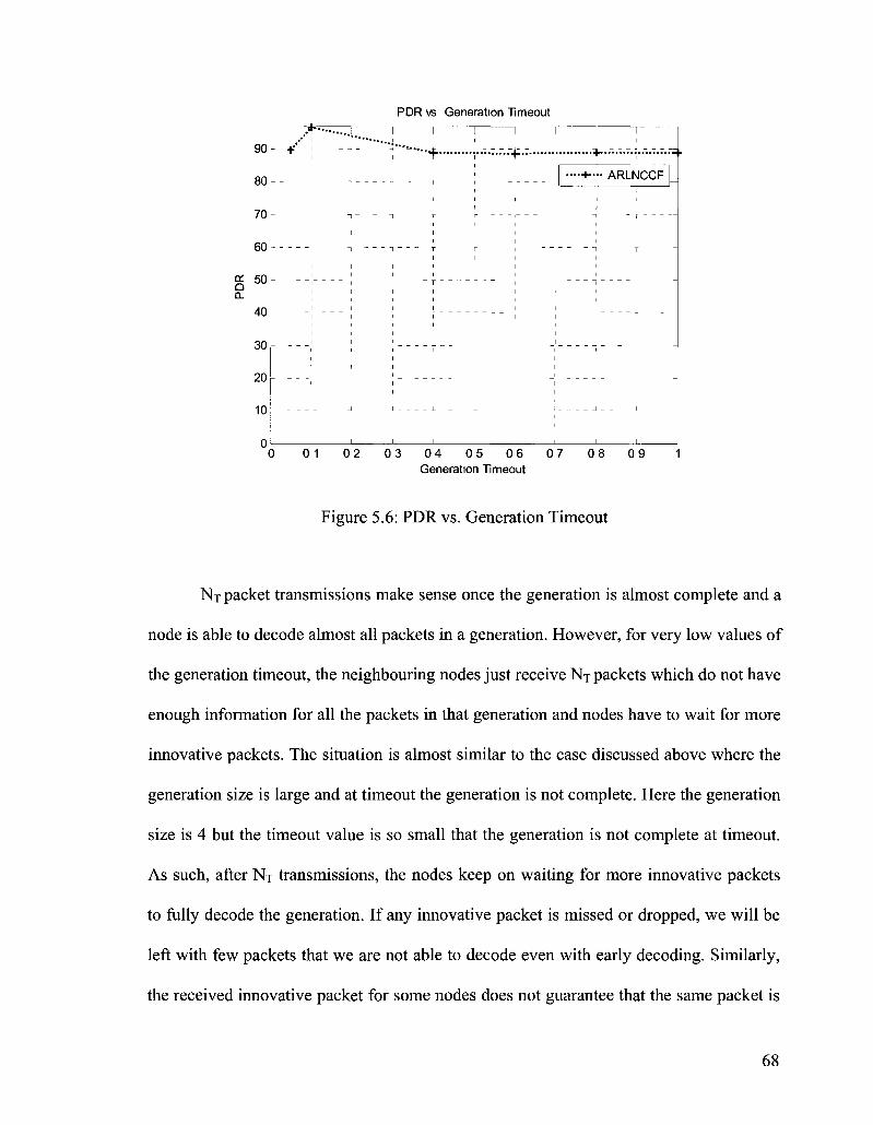
PDR vs Generation Timeout
l I I l I I
"""•"+ j--».».-+» +.r.r..r.L-..-..^. ' I ••••+•- ARLNCCF I
l r r i — i T
J L _ L I I 1
,_, . . . J I I I I I I
0 0 1 0 2 0 3 0 4 0 5 0 6 0 7 0 8 0 9 1 Generation Timeout
Figure 5.6: PDR vs. Generation Timeout
NT packet transmissions make sense once the generation is almost complete and a
node is able to decode almost all packets in a generation. However, for very low values of
the generation timeout, the neighbouring nodes just receive NT packets which do not have
enough information for all the packets in that generation and nodes have to wait for more
innovative packets. The situation is almost similar to the case discussed above where the
generation size is large and at timeout the generation is not complete. Here the generation
size is 4 but the timeout value is so small that the generation is not complete at timeout.
As such, after NT transmissions, the nodes keep on waiting for more innovative packets
to fully decode the generation. If any innovative packet is missed or dropped, we will be
left with few packets that we are not able to decode even with early decoding. Similarly,
the received innovative packet for some nodes does not guarantee that the same packet is
68
90
80
70
60
£ 50 Q CL
40
30
20
10

innovative for other nodes as well. If some generations receive all innovative packets by
chance, nodes are able to decode the generation fully. However some of the packets are
decoded with a delay after receiving innovative packets later on. This results in higher
latency as shown in Figure 5.7. At a timeout value of 0.1 second, the PDR improves and
latency is reduced. It is however observed that we have a higher number of MAC
transmissions in order to achieve higher PDR and lower latency.
There needs to be a balance between generation size as well as timeout value.
Once we further increase the generation timeout value, the PDR declines to around 90%
and then remains constant. Similarly, the latency starts to increase slightly as the timeout
value increases. The reason for this behavior is that the timeout value is set such that at
this value, even if the generation is not complete due to either delays or drop of packets,
the nodes need to re-encode and transmit NT packets. For higher timeout values, if the
generation is not complete by any chance before the timeout value, the nodes keep on
waiting for the timeout to expire before they can re-encode and transmits the packets for
that generation. This causes higher latency.
Figure 5.8 shows MAC transmissions as a function of Generation Timeout. For
higher timeout values, the nodes retransmit only when the generation is complete. The
reason for this is that most of the generations get completed before the timeout expires.
The generation is complete once it has received all innovative packets and the number of
rows equals the number of columns in the decoding matrix. This causes fewer MAC
transmissions but results in slightly lower PDR and slightly higher latency. In a nutshell,
these parameters strike a compromise between one performance metric and another.
69

Latency vs Generation Timeout 1
09
08
07h
06 >» CJ
I 05 CO
_ i
04
03
02
01
0 0 01 02 03 04 05 06 Generation Timeout
07 08 09
Figure 5.7: Latency vs. Generation Timeout
MAC Transmissions \s Generation Timeout
O <
01 02 03 04 05 06 07 08 09 Generation Timeout
Figure 5.8: MAC Transmissions vs. Generation Timeout
70

5.4.3 Early Decoding
01-Source Scenarios - Varying data rate
Scenario
(01-Source (Static), Nodes 50 - Generation size 6, GD Threshold 2, Timeout 0.1)
As shown in Figure 5.9, there is almost no difference in PDR with and without
early decoding. The major impact is on the latency as shown in Figure 5.10. At very low
data rates, we see that it takes much longer time to complete the generations and as a
result the latency is quite high for cases that do not support early decoding. For very low
data rates, at a generation timeout of 0.1 second, very few packets are generated (fewer
than the generation size). After NT transmissions, the neighbouring nodes need to wait for
more innovative packets to fully decode the generation (without early decoding).
PDR \s Rate(STATIC - 01 Source)
09
08
07
06
g 05^ CL
04
03
02
01
0
n ; ;•
i
I
_
_ __
I i
' * -
_ _ J
. . . . :
i ~i
i i
- ' ; - , — : n
—if— Without Early Decoding -
4 1 4- 4_
_, + + h
- i -*• 1- t- —
i T T r
_ J 1 1 L
i 1 1 1
0 10 20 30 40 50 60 70 80 90 100 Rate (kbps)
Figure 5.9: PDR vs. Rate (kbps) - (Static - 01 Source)
71

With early decoding, we always get the chance to decode the sub-matrix.
However in the absence of early decoding, the nodes receive very few packets after the
timeout for very low data rates and keep on waiting for more innovative packets. Since
the data rate is very low, the innovative packets also arrive at a very slow rate. Once all
the innovative packets arrive and a generation is complete, the node decodes the
generation successfully.
Latency vs Rate(STATIC - 01 Source)
0) TO
0
—•— With Early Decoding -^— Without Early Decoding
_J L_
0 10 20 30 40 50 60 70 80 90 100 Rate (kbps)
Figure 5.10: Latency vs. Rate (kbps) - (Static - 01 Source)
Overall, this leads to a PDR which is almost the same as with early decoding but
results in very large decoding delays. As the data rate increases to beyond 50 kbps, higher
data rates cause the generations to also complete quickly and the difference between with
and without early decoding becomes less significant. The difference still exists but
reduces to 0.05 - 0.15 second as shown in Figure 5.10.
72
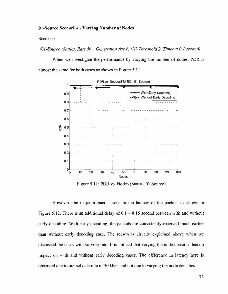
01-Source Scenarios - Varying Number of Nodes
Scenario
(01-Source (Static), Rate 50 — Generation size 6, GD Threshold 2, Timeout 0.1 second)
When we investigate the performance by varying the number of nodes, PDR is
almost the same for both cases as shown in Figure 5.11.
1
09
08
07
06
g 05 0.
04
03
02
01
PDR vs Nodes(STATIC - 01 Source)
* - ! r-+-
-
L ' *
--
- - -
_ . J
i
1 L ^ _ J 1 4 IAI 1.1. I - - i r^ l
—^— Without Early Decoding J 1 i L
1 T T 1 "
J ± _ _ ± L .
I I I
0 10 20 30 40 50 60 70 80 90 100 Nodes
Figure 5.11: PDR vs. Nodes (Static - 01 Source)
However, the major impact is seen in the latency of the packets as shown in
Figure 5.12. There is an additional delay of 0.1 - 0.15 second between with and without
early decoding. With early decoding, the packets are consistently received much earlier
than without early decoding case. The reason is already explained above when we
discussed the cases with varying rate. It is noticed that varying the node densities has no
impact on with and without early decoding cases. The difference in latency here is
observed due to our set data rate of 50 kbps and not due to varying the node densities.
73

Latency vs Nodes(STATIC - 01 Source) 04
0 35
03
^ 0 25 CJ
c £ TO
-1 02
0 15
01
0 05
0 10 20 30 40 50 60 70 80 90 100 Nodes
Figure 5.12: Latency vs. Nodes (Static - 01 Source)
04-Source Scenarios - Varying Rate
Scenario
(04-Source (Static), Nodes 50 - Generation size 4, GD Threshold 1, Timeout 0.1)
The results for scenarios with 4 sources are almost similar to those of single
source scenarios with the difference that after 25kbps rate, the latency is almost the same
for both cases of with and without early decoding as shown in Figure 5.14. Before the 25
kbps data rate, the case without early decoding has much higher latency due to low data
rates. It takes more time to complete the generation fully and then decode. Early decoding
shows a steady performance and shows no impact due to different data rates. The reason
for this behavior is already explained when discussing the single source scenarios.
74
• With Early Decoding —^— Without Early Decoding
- - *

PDR vs Rate (STATIC - 04 Source) 1
09
08
07
06
g 05[ CL
04
03
02
01
0
I
_
__ _ —
1
-J
- - - - - - -
~l
I I
1 1 ! 1
J 1 1 L '
—ic— Without Early Decoding
— i _ .(- +
- i-
i i
-i -
1-
1-
1 H
1
1 1
! 1
'
0 5 10 15 20 25 30 35 40 45 50 Rate (kbps)
Figure 5.13: PDR vs. Rate (kbps) - (Static - 04 Source)
35 Latency vs Rate(STATIC - 04 Source)
A V
25
CJ c CD
1 5
05
0
—•— With Early Decoding -^— Without Early Decoding
> =*——41
0 5 10 15 20 25 30 35 40 45 50 Rate (kbps)
Figure 5.14: Latency vs. Rate (kbps) - (Static - 04 Source)

04-Sources Scenarios - Varying Number of Nodes
Scenario
(04-Source (Static), Rate 25 - Generation size 4, GD Threshold 1, Timeout 0.1 second)
Keeping the data rate at 25 kbps and varying the number of nodes, we observe
that there is a consistent additional delay between with and without early decoding cases
as shown in Figure 5.16. We are always able to decode the packets early and achieve
lower latency for different node densities.
PDR vs Nodes (STATIC - 04 Source)
09
08
07
06
g 05
CL
04
03
02
01
0 20 30 40 50 60
Nodes
^_,-L L " *
L 1 J.
J_ 4 _J
1 1 1 1
1 * i 1 « , r
* . i « i i i r - . j r-v i - _
—~A— Without Early Decoding 1
,
;
70 80 90 100
Figure 5.15: PDR vs. Nodes (Static - 04 Sources)
76
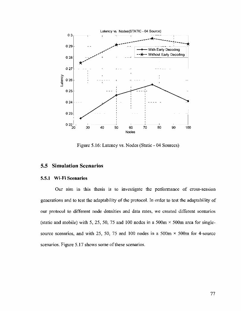
>> o c CD
0 3
0 29
0 28
0 27
0 26
0 25
0 24
0 23
Latency vs Nodes(STATIC - 04 Source)
0 22
1 1
. , • • -
* • • - •
i i i
A I A / . I L . 1 - - . 1 r-« i
—"A— Without Early Decoding
- - - -
--
-
20 30 40 50 60 70 80 90 Nodes
Figure 5.16: Latency vs. Nodes (Static - 04 Sources)
100
5.5 Simulation Scenarios
5.5.1 Wi-Fi Scenarios
Our aim in this thesis is to investigate the performance of cross-session
generations and to test the adaptability of the protocol. In order to test the adaptability of
our protocol to different node densities and data rates, we created different scenarios
(static and mobile) with 5, 25, 50, 75 and 100 nodes in a 500m x 500m area for single-
source scenarios, and with 25, 50, 75 and 100 nodes in a 500m x 500m for 4-source
scenarios. Figure 5.17 shows some of these scenarios.
77

05 nodes 25 nodes 350 600 r
200 400 X coordinates
50 nodes
200 400 X coordinates
100 nodes 600 600 r
600
200 400 X coordinates
200 400 X coordinates
600
Figure 5.17: Different Scenarios
It can be seen from Figure 5.17 that by increasing the number of nodes in the
network in the same area, we are in fact increasing the node density. Fewer
retransmissions are required per node in case of a dense network as there are more
neighbours available, contributing to the retransmissions. Later, we show through
simulations that our protocol is able to appropriately control the number of
retransmissions for different scenarios and exhibits steady behavior.
Also, we tested our protocol for different data rates. We selected 1 kbps, 50 kbps
and 100 kbps data rate for single-source scenarios and 1 kbps, 25 kbps and 50 kbps data
rate per source for 4-sources scenarios. Some of the common parameters for each
scenario are summarized in Table 5.3.
78

Traffic
Packet size
Area
Propagation model
InterFace Queue (IFQ)
Mobility
Model
Minimum speed
Maximum speed
Pause
Speed type
setdest version
Constant Bit Rate (CBR)
256 bytes
500 m x 500 m
2-ray ground
50
Random waypoint mobility model
2 m/s
lOm/s
0 sec
Uniform
Version 2
Table 5.3: Common Parameters
Based on the results in Section 5.4, we carefully selected the generation size of 6
for single-source scenarios. We did not select a higher value than 6 as it has impact on the
complexity of the protocol. Each coded packet carries a source address and sequence
number pair to uniquely identify each original packet. A bigger generation size implies
each coded packet has to carry more source address and sequence number pairs to
uniquely identify each original packet it is carrying, thus increasing the size of the coded
packet. We selected a generation size of 4 for multi-source scenarios with timeout value
set at 0.1 second. These values are selected based on the sensitivity of our protocol to
these values. We selected the optimal values that give the best performance in terms of
PDR and latency.
In case of mobility, we used the Random Way-point mobility model with 0
second pause time and minimum and maximum speed of 2 m/s and 10 m/s respectively.
We used the NS2 built-in function SETDEST to generate these scenarios.
79

Generation Size Number of nodes Data rate Gen timeout GD
Generation Size Number of nodes Data rate Gen timeout GD
Generation Size Number of nodes Date Rate Gen timeout GD
Generation Size Number of nodes Gen timeout GD
Hello interval (ARLNCCF, SMF
Single Source Scenarios 06 5-100 (Data rate fixed at 50 kbps) 1-100 kbps (Nodes fixed at 50)
0.1 second 2
04-Source Scenarios 04 25-100 (Data rate fixed at 25 kbps per source) 1-50 kbps (Nodes fixed at 50) 0.1 second 1
04-source Cross-session Scenarios 04 25-100 (Data rate fixed at 25 kbps per source) 1-50 kbps (Nodes fixed at 50) 0.1 second 1
100-source Cross-session Scenarios 04 100 (rate: 1 and 4 packets /source) 0.2 second 1
and BCAST)
10 sec for all Static Scenarios
2 sec for Mobile Scenarios for SMF and ARLNCCF
Table 5.4: Simulation Parameters
To test the multi-source scenario performance with and without cross-session
generations, we created 4-sources and 100-sources scenarios. We have modified the idea
presented in [16] to generate 100-sources scenario. GD threshold is set to 1 as each node
is a source and setting it to higher value will cause the generation size to grow rapidly in
80
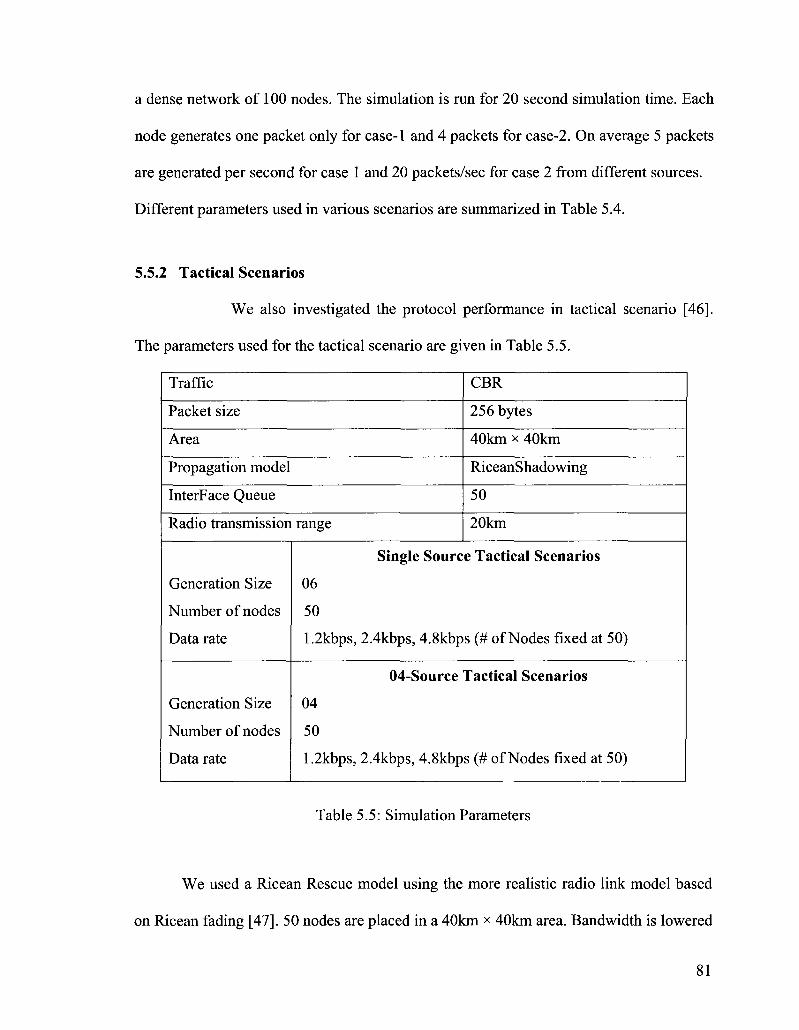
a dense network of 100 nodes. The simulation is run for 20 second simulation time. Each
node generates one packet only for case-1 and 4 packets for case-2. On average 5 packets
are generated per second for case 1 and 20 packets/sec for case 2 from different sources.
Different parameters used in various scenarios are summarized in Table 5.4.
5.5.2 Tactical Scenarios
We also investigated the protocol performance in tactical scenario [46].
The parameters used for the tactical scenario are given in Table 5.5.
Traffic
Packet size
Area
Propagation model
InterFace Queue
Radio transmission range
Generation Size
Number of nodes
Data rate
Generation Size
Number of nodes
Data rate
CBR
256 bytes
40km x 40km
RiceanShadowing
50
20km
Single Source Tactical Scenarios
06
50
1.2kbps, 2.4kbps, 4.8kbps (# of Nodes fixed at 50)
04-Source Tactical Scenarios
04
50
1.2kbps, 2.4kbps, 4.8kbps (# of Nodes fixed at 50)
Table 5.5: Simulation Parameters
We used a Ricean Rescue model using the more realistic radio link model based
on Ricean fading [47]. 50 nodes are placed in a 40km x 40km area. Bandwidth is lowered
81

to 128kbps and the radio transmission range is set to 20km. The carrier sense range is set
to the transmission range. SMF and simple flooding are selected for comparison. We
tested the protocols for both static and mobile scenarios.
Mobility in tactical scenarios [46]
Some nodes in the tactical scenario move according to the Random Waypoint
mobility model and some according to Reference Point Group Mobility Model, but their
velocity depends on the group a node belongs to. Of the 50 nodes, 3 nodes, representing
command-and-control centers, are nearly stationary. Seven nodes move individually
around the whole simulation area based on the Random Waypoint mobility model, with
speed randomly selected between 30km/h and 70km/h and 0 pause time. The remaining
40 nodes are grouped into 4 sets often nodes each, moving as a group. Each group of 10
nodes moves according to the Reference Point Group Mobility Model, where the
reference point moves with a speed randomly selected between 30 and 70 km/h and 0
pause time.
Within each group, nodes can deviate from the reference point by +/- 1 km in
each direction. In addition, each of the four groups is assigned to work in one quadrant of
the simulation area, with the quadrants slightly overlapping. For example, group one
works in the quadrant bounded by (0, 0) and (22 km, 22 km); group 2 works in a quadrant
bounded by (0, 18 km) and (18 km, 40 km), group three is within the quadrant bounded
by (18 km, 0) and (40 km, 22 km), and finally group 4 operates within the quadrant
bounded by (18km, 18km) and (40km, 40km).
82

In this chapter we have investigated the sensitivity of our protocol to generation
timeout and generation size. We also compared the performance with and without early
decoding by simulations. We showed that early decoding plays an important role in
reducing latency. Similarly, the simulations parameters and scenarios are explained in
detail. These scenarios are used to test the adaptive performance as well as the multi-
source coding feature of our protocol. The results for the above scenarios are discussed in
the next two chapters.
83

Chapter 6
Adaptive Performance
Our main aim in this chapter is to investigate the performance of our protocol by
varying the data rate as well as node density. The adaptive performance is analyzed for
static, mobile, as well as tactical scenarios. For each scenario, we investigated the
performance of our protocol compared to SMF, probabilistic flooding, BCAST and
simple flooding. The performance metric selected are PDR, latency and MAC
transmissions. First, the results for static scenarios are discussed for 01-source and 04-
sources. Later on, results for mobile and tactical scenarios are given with explanation.
6.1 Static Scenarios 01-Source
Figure 6.1 shows that as the data rate increases, the PDR for simple flooding and
BCAST drops significantly. ARLNCCF performs much better than simple flooding,
probabilistic flooding and BCAST as the data rate increases. However the PDR
performance drops slightly compared to SMF for higher rates. We have calculated 95%
confidence interval for all PDR plots where the difference between ARLNCCF and SMF
is less obvious. Further explanation about confidence intervals is provided in Section 6.7.
We also note that due to the generation timeout concept in our protocol, which is set at
0.1 second, there is always an inherent delay which is obvious in Figure 6.2. For lower
data rates, the delay is around 0.18 second which slightly increases to 0.25 second for our
protocol. Probabilistic flooding and SMF induce less delay compared to other protocols.
84

SMF shows the best performance in terms of PDR, low latency and fewer MAC
transmissions.
When comparing MAC transmissions, we need to explain the trend in more detail.
Figure 6.3 show that BCAST has fewer MAC transmissions than ARLNCCF and SMF.
However, when we compare the PDR for BCAST in Figure 6.1, it is much poorer than
SMF and ARLNCCF. The reason for the low number of MAC transmissions for BCAST
is due to packet drops in the InterFace Queue (IFQ) of the source itself. Due to channel
unavailability, the protocol drops the source packets at the queue and does not attempt to
deliver them. As a result there are fewer MAC transmissions but very low PDR as well.
Packet drops for the different protocols are shown in Figure 6.4.
PDR vs. Rate (STATIC - 01 Source)
a: a 0-
06
05
04
Confidence Interval (at 50 kbps) Static (SMF/ARLNCCF)
99 8 0 - 9 9 91 97 38 - 99.49
••»-••• BCAST - •— ARLNCCF
— * — FLOODING —Eh- Prob FLOODING
V SMF
0 10 20 30 40 50 60 70 80 90 100 Rate (kbps)
Figure 6.1: PDR vs. Rate (kbps) - (Static - 01 Source)
85

o c 0)
1 8
1.6
1.4
1.2
1
0 8
0 6
0 4
0.2
n
_ —
Latency vs. Rate (STATIC - 01 Sources)
• • • I — - BCAST
••*tf— FLOODING
- B - - Prob FLOODING
-^— SMF
: Ax i i ' I - 3* -I X -I -1- r - 1 i • V i i / v. i . ' , \
: X : :---' : / -- — •!-- X. -\-—
-l / - i , -!-X-i / i i i i > . j .
/ i i I I . . . • • i (
i y | _ _ _i 4 - - „ . I , . - -I / I . . • • ' I
/ ' ..*•* ' / / _ | _ ^ j I _
/ , j . ' ' ' | ,
' ' I . • • * " I I / | 7 I i i
V l l I I V I I I I T
0 10 20 30 40 50 60 70 80 90 100 Rate (kbps)
Figure 6.2: Latency vs. Rate (kbps) - (Static - 01 Source)
x -|g5 MAC Transmissions vs. Rate (STATIC - 01 Source)
25
ce 2 c g CO (O
E <2 1 5
<
0.5
0
• - 4 - - BCAST — • — ARLNCCF — * — FLOODING ~ B ~ Prob FLOODING
V SMF
B" '"
1 * " " .:.¥•""" i
0 10 20 30 40 50 60 70 80 90 100 Rate (kbps)
Figure 6.3: MAC Transmissions vs. Rate (kbps) - (Static - 01 Source)
86

12000
10000
8000
IFQ Drops vs. Rate (STATIC - 01 Source)
in o. P Q 6000 O
4000
2000
•+-••• BCAST -#— ARLNCCF
-•-A— FLOODING — B - - Prob FLOODING
V SMF
."•">'
°W^
-.;#- -
1 — j . . - 1 1 1 1 »
0~ 10 20 30 40 50 60 70 80 90 100 Rate (kbps)
Figure 6.4: IFQ Drops vs. Rate (kbps) - (Static - 01 Source)
Overall, comparison for the single source static scenario shows that SMF and
ARLNCCF achieve much higher PDR compared to other protocols with very few MAC
drops. Probabilistic flooding is better than BCAST and simple flooding but the optimal
probability value for retransmission needs to be determined for each scenario based on
different data rate and number of nodes, which is not a practical approach. The optimal
probability values vary from 0.5 - 0.1 for data rates of 1 kbps to 100 kbps respectively.
Similarly as we increase the node densities, a lower probability of retransmission is
required to achieve maximum performance.
In Figures 6.5 to 6.8, the number of nodes is varied from 5 to 100 in the same
geographical area. Generation timeout is set to 0.1 second and generation size is 6 for
ARLNCCF for single-source scenarios. It is observed that ARLNCCF shows steady
performance for all node densities by controlling the number of retransmissions. The
87

PDR performance is best for SMF and then ARLNCCF. The latency is around 0.23
seconds for ARLNCCF, which also remains steady for different node densities as shown
in Figure 6.6. Due to the generation timeout value in our protocol, the latency is higher
compared to SMF and probabilistic flooding. Referring to Figure 6.7 and 6.8, a trend
similar to the one when varying the data rate discussed above is seen for the MAC
transmissions and IFQ drops. BCAST and simple flooding have the highest IFQ drop
rate. Our protocol shows almost zero IFQ drops, similar to SMF and probabilistic
flooding, as shown in Figure 6.8.
0.9
0.8
g 07
06
0 5
04
PDR vs. Nodes(STATIC - 01 Sources) V " . j i V i i y
r , - -1~A ,
BCAST - •— ARLNCCF
• * — FLOODING -EJ-- Prob FLOODING -V—SMF
[ ]
- * - . . Confidence Interval (# of Nodes 501
Static (SMF/ARLNCCF) 99.80 -- 99.91 97.38 -- 99.49
'""*
0 10 20 30 40 50 60 70 80 90 100 Number of nodes
Figure 6.5: PDR vs. Nodes (Static - 01 Source)
88
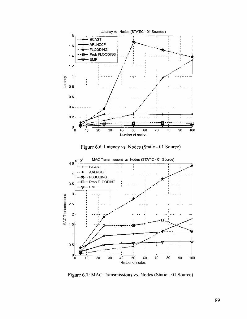
1 8
1 6
1.4
1 2
1
0 8
0 6
0 4
0 2
0
Latency vs Nodes (STATIC - 01 Sources)
••+•••• BCAST
- • — ARLNCCF
• • * — FLOODING
- B - - Prob FLOODING
- V — S M F
* - - .
• - * • - ; .
0 10 20 30 40 50 60 70 80 90 100 Number of nodes
Figure 6.6: Latency vs. Nodes (Static - 01 Source)
4 5
4
3.5
3
2 5
2
1 5
1
0 5
0
x i o 5 MAC Transmissions vs Nodes (STATIC - 01 Source)
- I — • BCAST
- 4 — ARLNCCF
• * — FLOODING
- B - - Prob FLOODING
- V — SMF
0 10 20 30 40 50 60 70 80 90 100 Nunber of nodes
Figure 6.7: MAC Transmissions vs. Nodes (Static - 01 Source)

2500
2000
1500 </> Q.
8 Q O 1000
500
IFQ Drops vs Nodes (STATIC - 01 Source)
•••*—• BCAST
- • — ARLNCCF
• • * — FLOODING
- H - - Prob FLOODING
-^—SMF
.+•*
.*-r A -1 '•
t T
,jjf I
0 10 20 30 40 50 60 Nodes
.+•
r -«|i-
70 80 90 1
Figure 6.8: IFQ Drops vs. Nodes (Static - 01 Source)
In summary, varying the node density from 5 to 100, ARLNCCF and SMF show
steady performance and there is no effect on the performance of the protocols as the node
density increases. For probabilistic flooding, we pre-determined the optimal value of
probability of retransmission for different node densities. Still we find its performance in
terms of PDR is lower than ARLNCCF and SMF. ARLNCCF and SMF are able to
control the number of retransmissions by neighbour knowledge (Although both use
different methods to determine the optimal number of required retransmissions), as a
result there is no impact observed by varying node densities. Our protocol has an
additional delay due to generation timeout but node density has no impact on this delay.
90

6.2 Static Scenarios 04-Sources
For 4-source static scenarios, generation timeout is set to 0.1 second for a
generation size of 4 for ARLNCCF. The PDR and latency performance is consistent with
the results obtained for the single source scenarios. As shown in Figure 6.9, at 50kbps per
source, the PDR drops to around 83 % for ARLNCCF and around 76% for SMF. The
main reason for this drop is that each source is generating data at the rate of 50 kbps and
the accumulative data rate of 200 kbps for 4 sources causes many MAC transmissions, as
seen in Figure 6.11. The wireless channel is always occupied and many packets do not
get the chance to be transmitted and are dropped at the InterFace Queue (IFQ) of the
source node as shown in Figure 6.12. SMF has the minimum latency, which increases to
around 0.2 seconds as the data rate increases as shown in Figure 6.10. Our protocol has a
latency of around 0.24 seconds, which remains consistent as the data rate increases.
PDR vs Rate (STATIC - 04 Sources)
Confidence Interval (at 25 kbps) Static (SMF/ARLNCCF)
0 5 L 98 3 3 - 9 9 30 1 96 06 - 97 57
04
03
02
0 5 10 15 20 25 30 35 40 45 50
Rate (kbps)
Figure 6.9: PDR vs. Rate (kbps) - (Static - 04 Sources)
91
BCAST •ARLNCCF
—*— FLOODING — B - - Prob FLOODING
V SMF
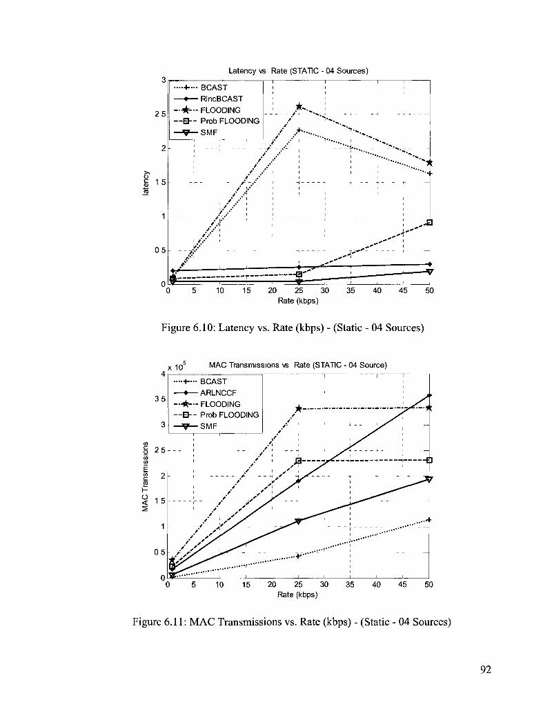
Latency vs Rate (STATIC - 04 Sources) o
25
2
>> o c 1 5 TO
1
05
n
•-•»—• BCAST
— * — FLOODING
— H - - Prob FLOODING V SMF
-1 j
/ . / - i - - - / - - . -
/ / / .•' ' i ' •' I
/ / 7,V , '*.•'
/ . • ' i
* ' . ' i
i / . • ' i
-$' <•' '
J?
tf zjzr~r~:
J
/ y .•
- / - - V -f
/
1
1 1 1 1 1
/ ^ "X-.-1 - + - - 4 - 1
V x . ^ * x .
.*• >-^ •* ' ' ' '*•...
'^>. ; ; , > i i i " • • • ] .
i 1 -t- - - + - - t- —
1 '
+ * ' •
**
- i 1 T > ^ » ^ - T r —
n--*" ' - ^ -v" -"™ '
0 5 10 15 20 25 30 35 40 45 50 Rate (kbps)
Figure 6.10: Latency vs. Rate (kbps) - (Static - 04 Sources)
x 1Q5 M A C Transmissions vs Rate (STATIC - 04 Source)
3 5
o CO CO
E co c SO
% 15
0 5
0
- •+- • • • BCAST
— • — ARLNCCF
— * — FLOODING
~ B ~ Prob FLOODING
V SMF
a — --H
0 5 10 15 20 25 30 35 40 45 50 Rate (kbps)
Figure 6.11: MAC Transmissions vs. Rate (kbps) - (Static - 04 Sources)

x 10 IFQ Drops vs Rate (STATIC - 04 Source)
Figure 6.12: IFQ Drops vs. Rate (kbps) - (Static - 04 Sources)
Figure 6.11 shows that BCAST has the lowest number of MAC transmissions but
the reason for this is that BCAST does not attempt to deliver most of the packets due to
IFQ drops as shown in Figure 6.12. Our protocol has more MAC transmissions for 4
source scenarios for higher data rates with Minimum IFQ drops.
SMF shows the best performance with higher PDR and fewer MAC transmissions
with minimum IFQ drops. Our protocol has the best PDR at a data rate of 50 kbps per
source but at the cost of a higher number of MAC transmissions.
93

The next series of results from Figure 6.13 to 6.16 are for 4-source static scenarios
when varying the number of nodes and hence the network density. The rate is fixed at
25kbps per source. The generation timeout is 0.1 second with a generation size set to 4.
The number of nodes is increased from 25 to 100 in the same geographical area. SMF
and ARLNCCF have the best PDR but SMF achieves a slightly higher PDR with fewer
MAC transmissions. Latency for ARLNCCF increases from 0.18 second for 25 nodes to
0.21 second for 100 node scenarios.
The overall performance of ARLNCCF for static scenarios is that it shows steady
performance for both 01-source and 04-sources. The protocol adapts itself well to
different data rates as well as different node densities. However, our protocol achieves
this performance at the cost of more number of MAC transmissions compared to SMF,
especially for 04-source scenarios with a data rate of 50 kbps per source.
PDR vs. Nodes (STATIC - 04 Sources)
0.9
0 8
0 7
O a.
0 6
0 5
0 4
••+••• BCAST
- • — ARLNCCF
• * — FLOODING
- B - - Prob FLOODING
- V — S M F
"*****-~«
Confidence Interval (# of Nodes 50) Static (SMF/ARLNCCF)
98.33 - 99 30 96.06 - 97.57
20 30 40 50 60 70 80 90 Nunber of nodes
Figure 6.13: PDR vs. Nodes (Static - 04 Sources)
100
94
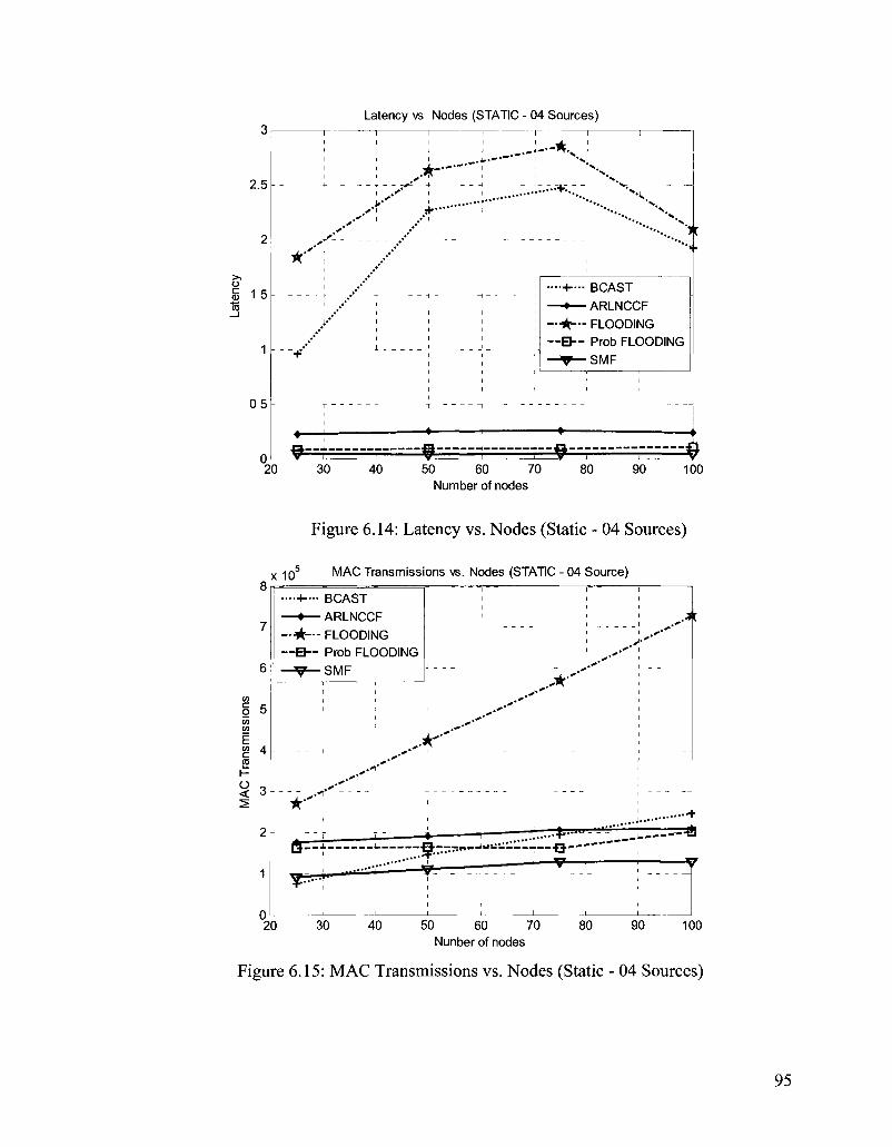
2.5
0 5
Latency vs Nodes (STATIC - 04 Sources)
. : - - * , . - • ' • •
*••
*--t r f-
•..-..-+-.•
*••• ***. ••-.. n
• • • • • I — - BCAST
— » — ARLNCCF
- - * — FLOODING
- - B - - Prob FLOODING
V SMF
* =* 0 20 30 40 50 60 70 80 90 100
Number of nodes
8
Figure 6.14: Latency vs. Nodes (Static - 04 Sources)
x -|05 MAC Transmissions vs. Nodes (STATIC - 04 Source)
< 3
••4—• BCAST
- • — ARLNCCF
• • * — FLOODING
- H ~ Prob FLOODING
- ^ — S M F
,.*"'
• ''
..*
6—j. J «.___„„ J rn^=*J
-•a—*
20 30 40 50 60 70 80 90 100 Nunber of nodes
Figure 6.15: MAC Transmissions vs. Nodes (Static - 04 Sources)
95

x 10 IFQ Drops vs. Nodes (STATIC - 04 Source)
^T.
CO Q.
p Q 3 O
* • * "
....+...
- • * - •
— H - -
BCAST
• ARLNCCF
- FLOODING
Prob FLOODING
•SMF
-K"
• - - - * .
—+
20 30 40 50 60 70 80 90 1 Nodes
Figure 6.16: IFQ Drops vs. Nodes (Static - 04 Sources)
6.3 Mobile Scenarios 01-Source
The next series of results from Figure 6.17 to 6.24 show the results for 01-source
mobile scenarios and results are presented for different data rates and node densities.
Generation timeout is set to 0.1 seconds with a generation size of 6 for single-source
scenarios for ARLNCCF. SMF and ARLNCCF have the best PDR performance. As
shown in Figure 6.17, ARLNCCF performs slightly better than SMF for lower data rates.
As the data rate increases, PDR for ARLNCCF starts to decline slightly to around 95%.
Similarly, Figure 6.18 shows that latency varies from around 0.16 second to 0.20 second
as the data rate increases.
96
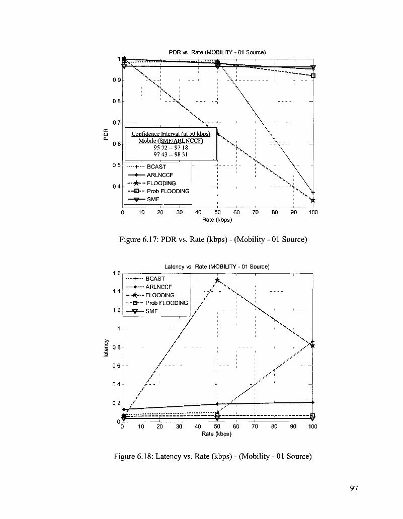
PDR vs Rate (MOBILITY - 01 Source)
a: a a.
07
06
0 5
04
Confidence Interval (at 50 kbps) ^ Mobile (SMF/ARLNCCF)
95 7 2 - 9 7 18 97 4 3 - 9 8 31
i T -
• - I— • BCAST — • — ARLNCCF — A — FLOODING - - E h - Prob FLOODING
V SMF
' X
- v 'X ,-
0 10 20 30 40 50 60 70 80 90 100 Rate (kbps)
Figure 6.17: PDR vs. Rate (kbps) - (Mobility - 01 Source)
1 6
1 4
1 2
1
08
06
04
02
0
Latency vs Rate (MOBILITY - 01 Source)
• - - I — - BCAST
— ^ — FLOODING —Eh- Prob FLOODING
V SMF
I I I I I
/ V i
- - / : - % - v i / •>. i
: x : / , - -i ^ X "
/ /-/
X .
1 X 1 1 x
t ^ N t 1 H
/ ' x • - / - - - - _, + ,. x'»t
/ i i i
/ i i / i i
t i i
/ ' / , / .-**'
/ i / i .» '
B , , i , s
Y I I i 1
4**
,** ,** yf'
1 I
1 U _ < •
j . 1 _ - ,
r , i i ! V 0 10 20 30 40 50 60 70 80 90 100
Rate (kbps)
Figure 6.18: Latency vs. Rate (kbps) - (Mobility - 01 Source)

x 1Q5 M A C Transmissions vs. Rate (MOBILITY - 01 Source)
CO c o CO CO
E CO
c 2 O < 2
2.5
2
1.5
1
0.5
....+..
— B -
• BCAST
-ARLNCCF
- FLOODING
- Prob FLOODING
- S M F
/
/ - i - - / ' , /*
i / * i / /
/' /
t /
I
I J I /
/
yf-
JL ' .
-I -1
- -1 - - - - ~l
1
4
+
T
1
-- +
4 -
T -
1
)
" T
i
-
-
0 10 20 30 40 50 60 70 80 90 100 Rate (kbps)
Figure 6.19: MAC Transmissions vs. Rate (kbps) - (Mobility - 01 Source)
10000
9000
8000
7000
6000
a 5000
4000
3000
2000
1000
IFQ Drops vs. Rate (MOBILE - 01 Source)
CO a. P
°F
••••+•••• BCAST — • — ARLNCCF —A— FLOODING — E - - Prob FLOODING
V SMF
i r
• -i - - / ' T
/' i
/" '
J. n ,• I
0 10 20 30 40 50 60 70 80 90 100 Rate (kbps)
Figure 6.20: IFQ Drops vs. Rate (kbps) - (Mobility - 01 Source)
98
Comparing Figure 6.19 to Figure 6.3, we observe that for mobiles scenarios, overall, all
protocols require fewer MAC transmissions to achieve the PDR as given in Figure 6.1
and Figure 6.17 respectively. SMF and ARLNCCF have almost zero IFQ drops compared
to BCAST and flooding.
The next series of results from Figure 6.21 to Figure 6.24 show the results
obtained by varying the node densities. For single source mobile scenarios, we observe
that ARLNCCF, SMF and probabilistic flooding show steady performance. However, for
probabilistic flooding we need to find the optimal value of probability of retransmissions
for each data point. So there is no adaptivity as far as probabilistic flooding is concerned.
For number of nodes set to 5, there is high probability that the network is not fully
connected, therefore we get lower PDR for all protocols as shown in Figure 6.21.
However, we observe that as the node density increases, the PDR improves.
Latency performance in Figure 6.22 show a similar trend to the results observed
before. The same inherent delay is observed due to generation timeout which is set at 0.1
second for ARLNCCF. SMF has the minimum delay. Flooding and BCAST have the
worst performance in terms of both PDR and latency as the number of nodes increases.
MAC transmissions for ARLNCCF are higher, as before, compared to SMF. The
protocol with the highest number of MAC transmission is simple flooding as shown in
Figure 6.23.
99

PDR vs. Nodes (MOBILITY - 01 Source)
0 9
0 8
g 07 n.
0 6
0 5
0 4
•••+•••• BCAST
— • — ARLNCCF
— * - • - FLOODING
— B - - Prob FLOODING
V SMF
Confidence Interval (# of Nodes 50) Mobile (SMF/ARLNCCF)
95 7 2 - 9 7 18 97 4 3 - 9 8 31
0 10 20 30 40 50 60 70 80 90 100 Nunber of nodes
Figure 6.21: PDR vs. Nodes - (Mobility - 01 Source)
1 6
1 4
1 2
1
o | 0 8
_ i
0 6
0 4
0 2
0
Latency vs Nodes (MOBILITY - 01 Source)
—+-••• BCAST
— * — ARLNCCF
— * - • - FLOODING
— H - - Prob FLOODING
V SMF 7
-4-^-
^1d^^%^^^^^^--r--r-^-i 3 0 10 20 30 40 50 60 70 80 90 100
Number of nodes
Figure 6.22: Latency vs. Nodes - (Mobility - 01 Source)

x i o 5 MAC Transmissions vs Nodes (MOBILITY - 01 Source)
CO 4 c o
O <
2
0
•-+-••• BCAST
CCF
—A— FLOODING
- - B - - Prob FLOODING
V SMF
- - I yf t*
. * * I
| ,e / /
* \ ^
i
; - i
• > "
I I I I
I I , .M I I , ^
I I , * * * ! 4- 4 - ^ 1-
1 * ' ,«*i i i
*" ' ' '
-i 4 1 +-
1 1 1 1
0 10 20 30 40 50 60 70 80 90 100
Nunber of nodes
Figure 6.23: MAC Transmissions vs. Nodes - (Mobility - 01 Source)
2500
2000
IFQ Drops vs Nodes(MOBILE - 01 Source)
1500 a. 2 Q O
1000
500
0
••••-»—• BCAST
— » — ARLNCCF
— * — FLOODING
- - B - - Prob FLOODING
V SMF
f
r .-+"
-m-0 10 20 30 40 50 60 70 80 Nodes
90 100
Figure 6.24: IFQ Drops vs. Nodes - (Mobility - 01 Source)
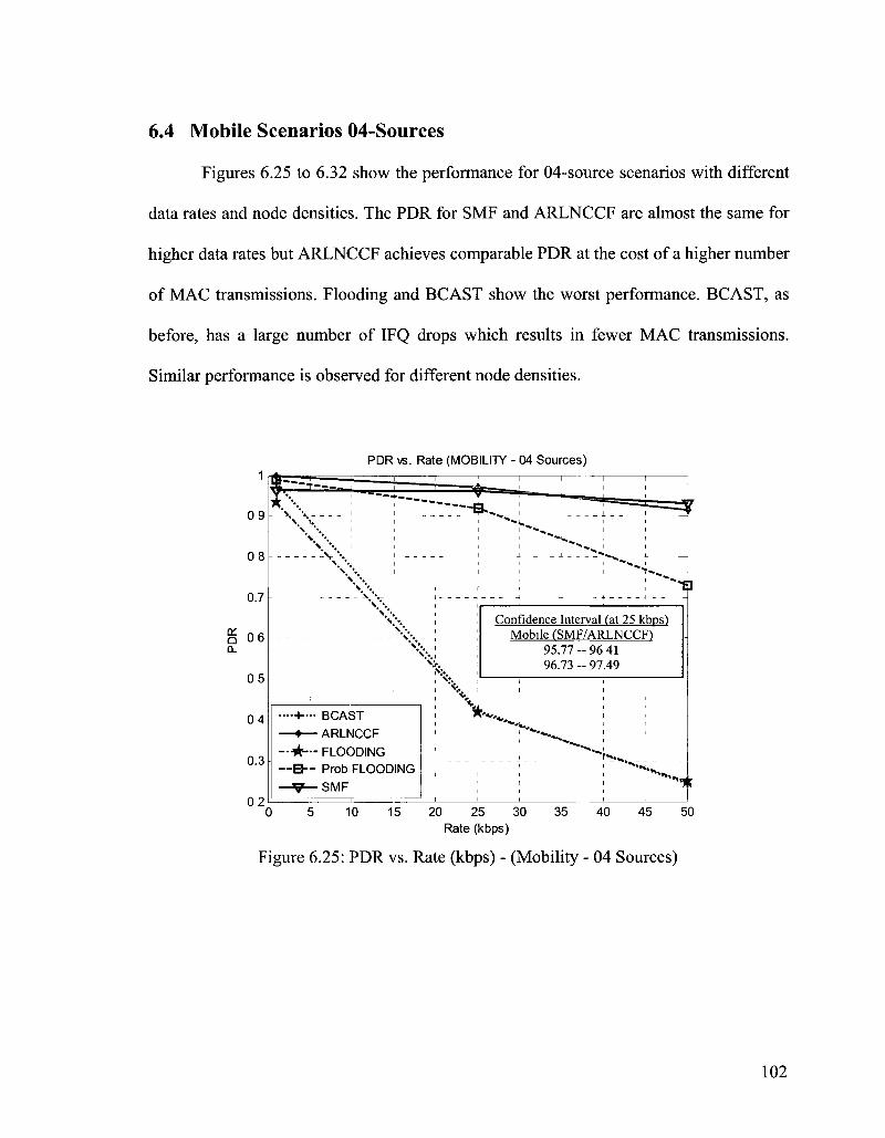
6.4 Mobile Scenarios 04-Sources
Figures 6.25 to 6.32 show the performance for 04-source scenarios with different
data rates and node densities. The PDR for SMF and ARLNCCF are almost the same for
higher data rates but ARLNCCF achieves comparable PDR at the cost of a higher number
of MAC transmissions. Flooding and BCAST show the worst performance. BCAST, as
before, has a large number of IFQ drops which results in fewer MAC transmissions.
Similar performance is observed for different node densities.
PDR vs. Rate (MOBILITY - 04 Sources) 1
09
08
0.7
g 06 o.
05
04
0.3
02
V . |
Confidence Interval (at 25 kbps) Mobile (SMF/ARLNCCF)
95.77-96 41 96.73 - 97.49
- • 4 - - BCAST — • — ARLNCCF —*lf— FLOODING - - B - - Prob FLOODING
V SMF
- t^-*'*.,-' ^ . .
0 10 15 20 25 30 35 40 45 50 Rate (kbps)
Figure 6.25: PDR vs. Rate (kbps) - (Mobility - 04 Sources)
102

Latency vs Rate (MOBILITY - 04 Sources)
CD
IS
1.8
1.6
1.4
1 2
1
0 8
0 6
0.4
0 2
0
• - • I — - BCAST — • — ARLNCCF — A — FLOODING — H - - Prob FLOODING
V SMF
/ .+-. >••..
/ /
-£'
*t £_ *
0 5 10 15 20 25 30 35 40 45 50 Rate (kbps)
Figure 6.26: Latency vs. Rate (kbps) - (Mobility - 04 Sources)
x io5 MAC Transmissions vs Rate (MOBILITY - 04 Source)
35
o * o CO CO
E VJ 2 2 % 1.5
0.5
••••+-- BCAST — • — ARLNCCF — * — FLOODING —B- Prob FLOOD
V SMF
/ y / /
/ *
NG
X
/ / /
i T r i
J L X L
4 - k 4- —
I z*** I - _ _ _ —
^ i i . • * 1**
-i»*** _ _ 1 _ _ i __
i i i i
0 5 10 15 20 25 30 35 40 45 50 Rate (kbps)
gure 6.27: MAC Transmissions vs. Rate (kbps) - (Mobility - 04 Sources)

a. 5 e Q
2 4
x 10 IFQ Drops vs Rate (MOBILE - 04 Source)
••+-••• BCAST -4— ARLNCCF ••A-- FLOODING - B ~ Prob FLOODING -V—SMF
n r
y- T •
* «
-i / i / *
..*
10 15 20
.•+
30 35 40 45 Rate (kbps)
Figure 6.28: IFQ Drops vs. Rate (kbps) - (Mobility - 04 Sources)
09
08
07 a: Q Q_
06
05
04
* . .
PDR vs Nodes (MOBILITY - 04 Sources)
: $ : ~ B -
• T — B - r ^ T-.
* » 4 i
— I — - BCAST — • — ARLNCCF —A— FLOODING — B - - Prob FLOODING
V SMF
Confidence Interval (# of Nodes 50) Mobile (SMF/ARLNCCF)
95 77 - 96 41 96 73 - 97 49
^ ^ v
20 30 40 50 60 70 80 90 100 Nunber of nodes
Figure 6.29: PDR vs. Nodes - (Mobility - 04 Sources)

2
1 8
1 6
1 4
1 2
1
08
06
04
02
Latency vs. Nodes (MOBILITY - 04 Sources)
*••.,
0 20
J5=
• v . : : . - * - . . . .
'.Tjr
• - 4 - - BCAST — • — ARLNCCF —A— FLOODING —B— Prob FLOODING
V SMF
z$= * 30 40 50 60 70
Number of nodes 80 90
-•a
100
Figure 6.30: Latency vs. Nodes - (Mobility - 04 Sources)
x -|05 MAC Transmissions vs Nodes (MOBILITY - 04 Source)
CO
I 5 CO CO
E CO A c H
2 H < 3
-• I— • BCAST - « — ARLNCCF ••A— FLOODING -EJ-- Prob FLOODING -V—SMF
.-•*
. > '
. . * "
9=± : : b ^ - ^ - - " ' ' : — * r-
— &
20 30 40 50 60 70 Nunber of nodes
80 90 100
Figure 6.31: MAC Transmissions vs. Nodes - (Mobility - 04 Sources)

x 10 IFQ Drops vs Nodes (Mobility 04-sources)
35
3
25 CO Q. P Q 2 O LL
1 5
0 5 +••'
r**1''
20 30 40
.+•..
••+•••• BCAST
- • — ARLNCCF
• • * ^ - FLOODING
- B - - Prob FLOODING
- V — S M F
V - .
60 Nodes
• *
->—9—i 1 *J 70 80 90 100
Figure 6.32: IFQ Drops vs. Nodes - (Mobility - 04 Sources)
6.5 Tactical Scenarios 01-Source
From the results for static and mobile scenarios, we selected the best candidates,
SMF and ARLNCCF to be evaluated for tactical scenarios. Flooding is selected as a
baseline protocol for comparison. For the single source case, the PDR for ARLNCCF is
slightly better than SMF as shown in Figure 6.33. As the data rate increases from 1.2
kbps to 4.8 kbps, the PDR for ARLNCCF shows a slightly decreasing trend. Figure 6.34
shows that the latency for ARLNCCF is higher than SMF due to the generation timeout.
The number of MAC transmissions required to achieve this PDR increases with data rate
and at 4.8 kbps, SMF requires fewer MAC transmissions compared to ARLNCCF as
shown in Figure 6.35.
106

1
09
0.8
07
06
g 05 o.
04
03
02
01
0
PDR vs Rate (TACTICAL - 01 Source) i lit i i . . , i i
1
- • * -
—v-• FLOODING
SMF
•v<i7-'r"
Confidence Interval (at 2 4 kbps) Tactical (SMF/ARLNCCF)
92 1 7 - 9 5 75 98.56 - 99 99
1 5 25 3 35 Rate (kbps)
45
Figure 6.33: PDR vs. Rate (kbps) - (Tactical - 01 Source)
03
IS
0 5
0 45
0 4
0 35
0 3
0 25
0 2
0 15
0 1
0 05
0
Latency vs NodesfTACTICAL - 01 Source)
1 1 5
I I I
_ _ L ± _ _ _ i
J- 4- -L - I
f- 4 -i - i
t 1- s -
r T T — - ]
• 1 •
t
--A" FLOODING —V"-SMF
1 1 f- * *
V ' . . . . . . - - y - , . . . . _ . . - . . . --y
1 1 1 1 1 1 1
25 3 35 Rate (kbps)
4 5
Figure 6.34: Latency vs. Rate (kbps) - (Tactical - 01 Source)
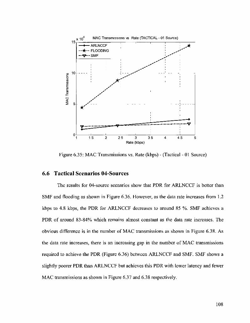
15 x -eg4 MAC Transmissions vs Rate (TACTICAL - 01 Source)
c o
E CO c
<
10
1 5 25 3 35 Rate (kbps)
- • • • • -
.'
ARLNCCF FLOODING SMF
I l A
i - <
: ^ i
I I +* I I
i-,/"'" J.. -! -x : A'
i i i i i i
4 5
Figure 6.35: MAC Transmissions vs. Rate (kbps) - (Tactical - 01 Source)
6.6 Tactical Scenarios 04-Sources
The results for 04-source scenarios show that PDR for ARLNCCF is better than
SMF and flooding as shown in Figure 6.36. However, as the data rate increases from 1.2
kbps to 4.8 kbps, the PDR for ARLNCCF decreases to around 85 %. SMF achieves a
PDR of around 83-84% which remains almost constant as the data rate increases. The
obvious difference is in the number of MAC transmissions as shown in Figure 6.38. As
the data rate increases, there is an increasing gap in the number of MAC transmissions
required to achieve the PDR (Figure 6.36) between ARLNCCF and SMF. SMF shows a
slightly poorer PDR than ARLNCCF but achieves this PDR with lower latency and fewer
MAC transmissions as shown in Figure 6.37 and 6.38 respectively.
108
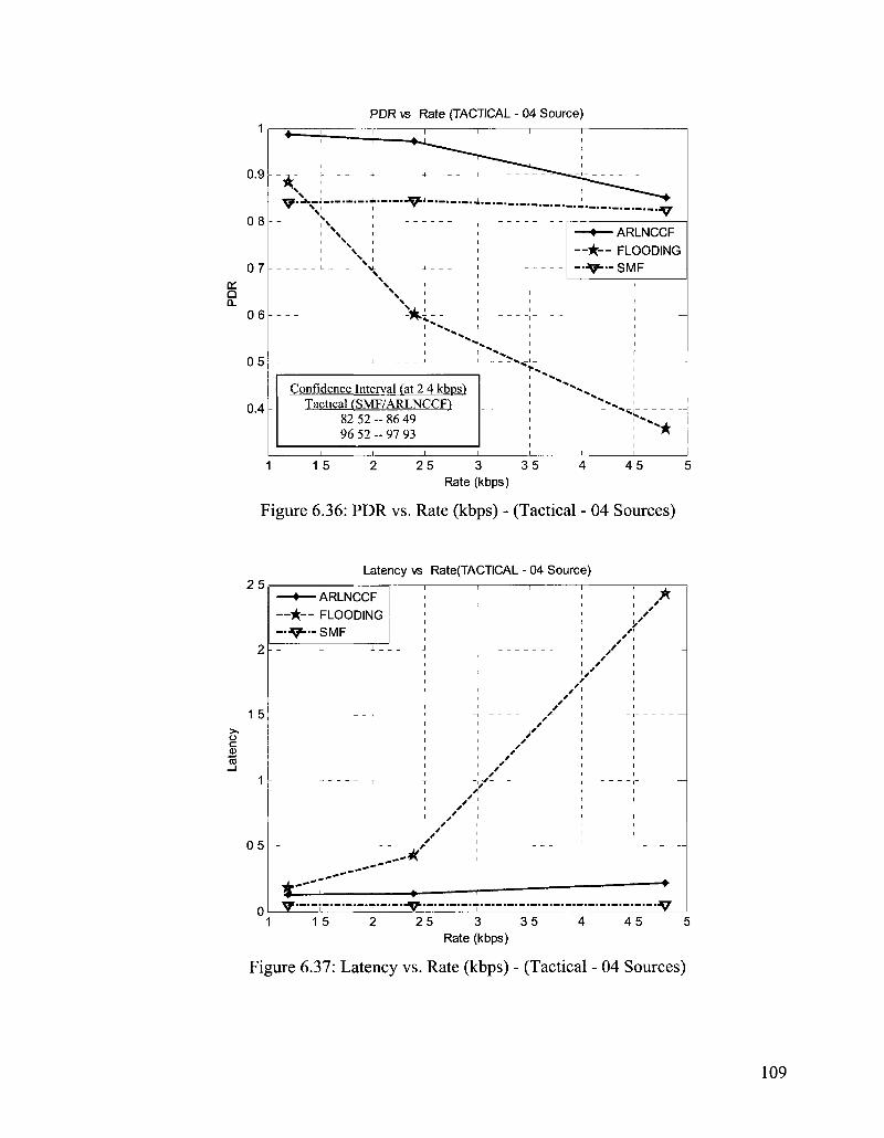
PDR vs Rate (TACTICAL - 04 Source)
or Q o.
0.9
08
07
06
05
0.4
*• 1 1
• X 1
- - \ X
1 \
' \ 1 \ 1 N \ i _ _ _ \
k X -1 \ 1
\ 1
\ '
: \
Confidence Interval (at 2 4 kbps) Tactical (SMF/ARLNCCF)
82 52 - 86 49 96 52 - 97 93
i i
I * «
— • — ARLNCCF —A— FLOODING — V - S M F
•*•»
-
" > *
1 15 2 25 3 35 4 45 5 Rate (kbps)
Figure 6.36: PDR vs. Rate (kbps) - (Tactical - 04 Sources)
25 Latency vs RatefTACTICAL - 04 Source)
o c CD
— • — ARLNCCF --A— FLOODING —V--SMF
Rate (kbps)
Figure 6.37: Latency vs. Rate (kbps) - (Tactical - 04 Sources)

x 105 MAC Transmissions vs Rate (TACTICAL - 04 Source) 25
2
E CO c 2 h-O 1 <
05
0 1 1.5 2 2 5 3 3 5 4 4 5 5
Rate (kbps)
Figure 6.38: MAC Transmissions vs. Rate (kbps) - (Tactical - 04 Sources)
6.7 Summary
Overall, ARLNCCF shows a steady performance for different nodes densities and
rates for both 01-source and 04-source scenarios. We tested the performance for quite
aggressive data rates of up to 100 kbps for 01-source scenarios and up to 50 kbps for 04-
source scenarios. Similarly, the number of nodes is increased from 5 to 100 nodes in the
same geographical area. ARLNCCF shows a steady performance in terms of both PDR
and latency but there is always some inherent delay due to the need to buffer packets to
generate encoding opportunities, which is bounded by the generation timeout. Our
protocol, when compared to flooding and BCAST, performs much better. As far as
comparison with probabilistic flooding is concerned, since probabilistic flooding is not
adaptive to changing scenarios, we need to determine the optimal value of probability of
retransmission for each data point considered. Even considering the optimal probability
110
--A" FLOODING —V--SMF
1 1
x * ^ i , ' i
X' :... r T i ~i
- *
i
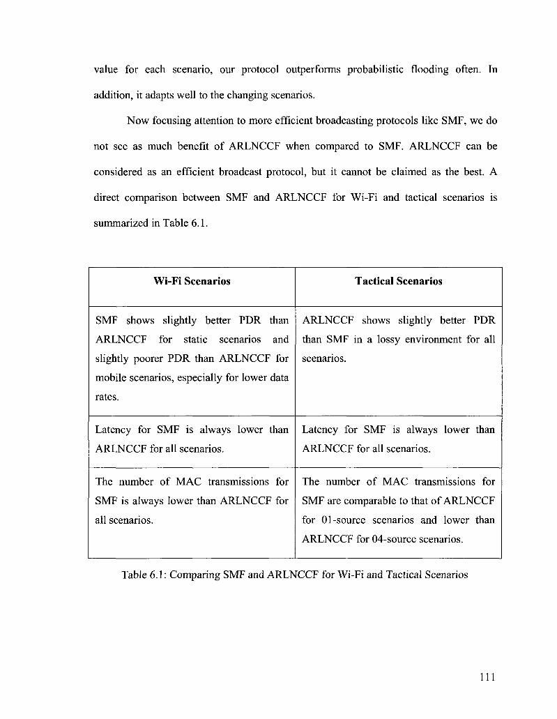
value for each scenario, our protocol outperforms probabilistic flooding often. In
addition, it adapts well to the changing scenarios.
Now focusing attention to more efficient broadcasting protocols like SMF, we do
not see as much benefit of ARLNCCF when compared to SMF. ARLNCCF can be
considered as an efficient broadcast protocol, but it cannot be claimed as the best. A
direct comparison between SMF and ARLNCCF for Wi-Fi and tactical scenarios is
summarized in Table 6.1.
Wi-Fi Scenarios
SMF shows slightly better PDR than
ARLNCCF for static scenarios and
slightly poorer PDR than ARLNCCF for
mobile scenarios, especially for lower data
rates.
Latency for SMF is always lower than
ARLNCCF for all scenarios.
The number of MAC transmissions for
SMF is always lower than ARLNCCF for
all scenarios.
Tactical Scenarios
ARLNCCF shows slightly better PDR
than SMF in a lossy environment for all
scenarios.
Latency for SMF is always lower than
ARLNCCF for all scenarios.
The number of MAC transmissions for
SMF are comparable to that of ARLNCCF
for 01-source scenarios and lower than
ARLNCCF for 04-source scenarios.
Table 6.1: Comparing SMF and ARLNCCF for Wi-Fi and Tactical Scenarios
111
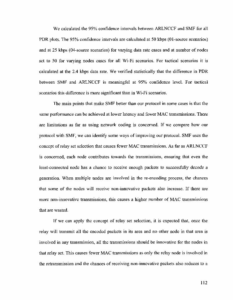
We calculated the 95% confidence intervals between ARLNCCF and SMF for all
PDR plots. The 95% confidence intervals are calculated at 50 kbps (01-source scenarios)
and at 25 kbps (04-source scenarios) for varying data rate cases and at number of nodes
set to 50 for varying nodes cases for all Wi-Fi scenarios. For tactical scenarios it is
calculated at the 2.4 kbps data rate. We verified statistically that the difference in PDR
between SMF and ARLNCCF is meaningful at 95% confidence level. For tactical
scenarios this difference is more significant than in Wi-Fi scenarios.
The main points that make SMF better than our protocol in some cases is that the
same performance can be achieved at lower latency and fewer MAC transmissions. There
are limitations as far as using network coding is concerned. If we compare how our
protocol with SMF, we can identify some ways of improving our protocol. SMF uses the
concept of relay set selection that causes fewer MAC transmissions. As far as ARLNCCF
is concerned, each node contributes towards the transmissions, ensuring that even the
least-connected node has a chance to receive enough packets to successfully decode a
generation. When multiple nodes are involved in the re-encoding process, the chances
that some of the nodes will receive non-innovative packets also increase. If there are
more non-innovative transmissions, this causes a higher number of MAC transmissions
that are wasted.
If we can apply the concept of relay set selection, it is expected that, once the
relay will transmit all the encoded packets in its area and no other node in that area is
involved in any transmission, all the transmissions should be innovative for the nodes in
that relay set. This causes fewer MAC transmissions as only the relay node is involved in
the retransmission and the chances of receiving non-innovative packets also reduces to a
112

very large extent. We expect that if the relay set mechanism is applied to ARLNCCF, it
will improve the performance of ARLNCCF in terms of fewer MAC transmissions, and
may allow it to efficiently support even higher data rates.
113

Chapter 7
Cross-Session Performance
In this chapter, we investigate the cross-session performance of our protocol. The
main aim is to see how much benefit we are getting in allowing inter-mixing of packets
from different sources in the same generation. We devised 100-source scenarios as well
as 04-source scenarios to investigate the cross-session performance, as described in
Chapter 5.
7.1 100-source Scenarios
In case of 100-source scenarios, 100 nodes are placed in a 500m * 500 m area.
Using the concept of GD threshold (GD = 1), we are able to control the generation size
growth. We observed that the generation size increased from 4 to 8 on average for some
generations we monitored closely. Without GD threshold, the generation size becomes
quite large in a dense network of 100 nodes where each node is a source. We observed
generation size growth up to 14 or more on average for some monitored generations if we
do not use the GD threshold concept. These scenarios are further classified into two
types.
1. Each source generates only a single packet during the course of simulation. In
the absence of cross-session generations, after the timeout period, since the
node generates only one packet, network coding plays no role as there is only
114

a single encoded packet. The protocol in this case deteriorates to a simple
forwarding approach without coding.
2. Each source generates 4 packets one after another so that at least the
generations are full before a timeout occurs, even in the case when we do not
allow for cross-session coding.
Table 7.1 shows the PDR performance for both mobile and static scenarios. It is
observed that for each case the PDR is better with cross-session generations. The results
are further verified via 95 % confidence intervals for each data point. We verified
through statistical analysis that the difference is statistically significant and not just due to
randomness of simulations.
Scenario
Mobile (1 packet per source)
Mobile (4 packets per source)
Static (1 packet per source)
Static (4 packets per source)
PDR (%)
No Cross-session
96.38 T95.7635 - 97.01451
87.97 T86.2704- 89.67161
95.60 T94.8930 - 96.32371
82.58 T80.1976-84.96641
Cross-session
99.53 T99.3257 - 99.73631
96.46 T95.6979-97.23151
99.05 T98.4170- 99.69701
93.01 [90.9638 - 95.07421
Table 7.1: PDR for 1 Packet and 4 Packets per Source
Table 7.2 shows the latency performance for both mobile and static scenarios.
There is a significant impact on latency when we allow generations to mix packets from
different sources (cross-session). For mobile scenarios with 1 packet per source, without
cross-session coding, the latency is 0.49 second. Whereas, allowing cross-session coding,
the latency is reduced to 0.15 second. In case we allow each source to generate 4 packets,
115

without cross-session coding, the latency is 0.32 second compared to 0.185 second for
cross-session coding. Similar observations are made for static scenarios. Again, for each
value, the 95% confidence interval is provided to verify our results statistically.
Scenario
Mobile (1 packet per source)
Mobile (4 packets per source)
Static (1 packet per source)
Static (4 packets per source)
Latency (ms)
No Cross-session
0.49 [0.4842 - 0.50581
0.32 [0.3163-0.33171
0.624 [0.6058 - 0.64221
0.457 [0.4363 - 0.4792]
Cross-session
0.155 [0.1459-0.16411
0.185 [0.1737-0.19631
0.22 [0.2154-0.23711
0.30 [0.2785 - 0.32351
Table 7.2: Latency for 1 Packet and 4 Packets per Source
7.2 4-Source Scenarios
Figures 7.1 to 7.4 show the cross-session performance of ARLNCCF for 4-source
scenarios. Each figure compares the cases with and without cross-session coding for
static and mobile scenarios. Figure 7.1 and Figure 7.2 compare the PDR and latency as a
function of the data rate and Figure 7.3 and Figure 7.4 compare the PDR and latency as a
function of the number of nodes. The results show that, for all cases, the cross-session
coding cases have always better PDR as well as lower latency compared to no cross-
session coding. As seen in Figure 7.2, as the data rate increases, the latency for no cross-
session coding increases significantly for both static and mobile scenarios. The 95%
confidence interval is calculated for a scenario with a date rate of 25 kbps for scenarios
where we vary the date rate and for the scenario with the number of nodes set to 50 where
we varied number of nodes.
116
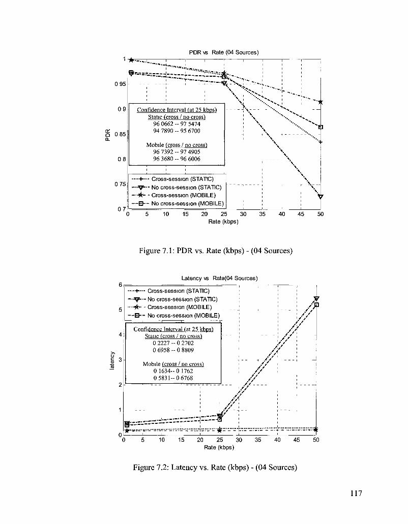
PDR vs Rate (04 Sources)
0 95
09
Q 0 85 o_
08
0 75
07
fpre.-.=J._--.__J_. " * « > r t j . - . _ . _
i " • • r - . ' i
"T J _ . .
Confidence Interval (at 25 kbps) Static (cross / no cross)
96 0662 - 97 5474 94 7890 - 95 6700
Mobile (cross / no cross) 96 7392 - 97 4905 96 3680 - 96 6006
" • > .
X ^H
....+.»• Cross-session (STATIC) — V " - No cross-session (STATIC) —At- - Cross-session (MOBILE) —El— No cross-session (MOBILE)
0 10 15 20 25 30 35 40 45 Rate (kbps)
50
Figure 7.1: PDR vs. Rate (kbps) - (04 Sources)
Latency vs Rate(04 Sources)
—.+.— Cross-session (STATIC) — ^ — No cross-session (STATIC) —A- • Cross-session (MOBILE) —Eh- No cross-session (MOBILE)
o
3 to
Confidence Interval (at 25 kbps) Static (cross / no cross)
0 2227 - 0 2702 0 6958 - 0 8809
Mobile (cross / no cross) 0 1634-0 1762 0 5831-0 6768
/ /
/ /
/ /
I / l l
w AA
/ / •* / ' i / i
//
1
o W--* ' » • •
AA\ n ^ y - -i •
1 JT '
: U : L : - ^ : ^ : I : - :,i-,:u-L--^^-,--L-:,",:-.-:,"L-,:i
0 10 15 20 25 30 35 40 45 50 Rate (kbps)
Figure 7.2: Latency vs. Rate (kbps) - (04 Sources)
117

0 98
0 97
0 96
Q 0 95 0_
0 94
0 93
0 92
PDR vs Nodes(04 Sources)
A
ffir'
A'-'
Q'
/ / .*••-—..
:-'---&
....+»•. Cross-session (STATIC) - • •V-- No cross-session (STATIC) —A- - Cross-session (MOBILE) —B— No cross-session (MOBILE)
20 30 40 50 60 70 80 90 100 Nodes
Figure 7.3: PDR vs. Nodes - (04 Sources)
The confidence interval for Figure 7.3 is given in Table 7.3 for the scenarios
nodes.
Confidence Interval (at Nodes 50) Static (cross / no cross)
96.0662 - 97.5474 94.6461 - 95.5877
Mobile (cross / no cross) 96.7392 - 97.4905 96.2402-96.6179
Table 7.3: Confidence Interval-PDR (04 Sources - 50 Nodes)

Latency vs Nodes(04 Sources) 08
07
06
o 05
04
..-v-^ • V - * - - . .
• ^ r -
-&.
••+•••• Cross-session (STATIC) ••V"- No cross-session (STATIC) ••A--- Cross-session (MOBILE) -El— No cross-session (MOBILE)
60 Nodes
100
Figure 7.4: Latency vs. Nodes (04 Sources)
The confidence interval for Figure 7.4 is given in Table 7.4 below at number of nodes set
to 50.
Confidence Interval (at Nodes 50) Static (cross / no cross)
0.2227 - 0.2702 0.5792 - 0.6952
Mobile (cross / no cross) 0.1634-0.1762 0.4749 - 0.6333
Table 7.4: Confidence Interval-Latency (04 Sources - 50 Nodes)
119

In a nutshell, the simulation results show that allowing cross-session coding has a
significant impact on PDR as well as latency, which is also statistically verified through
95%) confidence intervals. The concept of allowing cross-session generations in our
protocol plays an important role in multi-source scenarios. The results are more profound
for mobile scenarios.
120
Chapter 8
Conclusions and Future Work
8.1 Conclusions
In this thesis, we developed a wireless broadcast protocol based on Random
Linear Network Coding (RLNC). The following conclusions are drawn as a result of this
research work.
• Although there are many broadcast protocols developed so far, very few protocols
deal with multi-source RLNC based broadcast. Similarly, none of the RLNC-based
protocols are adaptive by design. They need parameters to control the number of
required transmissions. Probability-based methods require the optimal values of
probability of retransmission set beforehand to achieve better performance in
different scenarios.
• Using neighbour knowledge and the generation size, our protocol can effectively
calculate the number of rebroadcasts that are sufficient for all the nodes to decode the
coded packets. We tested our protocol in static, mobile and tactical scenarios for both
01-source and 04-source cases. Similarly, we investigated the performance by varying
the number of nodes as well as data rates in these scenarios. Our simulation results
demonstrate the potential of our algorithm to support wireless broadcast in adhoc
networks. We observe a steady performance of our protocol at different node
densities and data rates in all scenarios, thus making our protocol adaptive.
121
• During the simulations, we tested our protocol for very aggressive data rates (not used
in the literature before for RLNC based broadcast). As an example [91 used 40 kbps
and [15] used 50 kbps for single source scenarios. It is mentioned in [15] that their
RLNC based probabilistic broadcast algorithm has high packet loss for higher data
rates. We used up to 100 kbps for a single source and up to 25 kbps per source for 04-
source scenarios. It was observed that the PDR performance was not degraded. This
shows that by controlling the number of rebroadcasts, we are in fact able to achieve
better performance at higher data rates.
• When we compare our results with SMF, we observe that SMF achieves the same or
better PDR by using fewer MAC transmissions than our protocol in certain cases.
Similarly, our protocol has an inherent delay due to the generation timeout, as a result
latency is higher than SMF, but it does not increase with increasing node densities or
data rates and remains consistent.
• By using the concept of earlier decoding from previous research, we are able to
decode some of the original packets before the generation is complete. This greatly
reduces the decoding delays.
• Since our protocol is designed for multi-source environments and we allow packets
from different sources to be combined in the same generation (cross-session)
whenever possible, there is always a possibility that the generation size can grow to a
very large extent, especially for high data rates and multi-hop networks. This is
causing decoding complexity, decoding delays, and very large packet sizes. In order
to avoid this situation, we introduced the concept of Generation Distance (GD). GD
values can be set to control the source nodes entering their packets in the given
122

generation based on the distance (hops) from the generation origin. However as future
work we need to investigate further the impact of GD as well as devising more
efficient ways to control generation size.
• We have shown that our concept of cross-session generations plays an important role
in improving the PDR as well as reducing latency. We specifically designed 100-
source scenarios to test the cross-session concept. Similarly, we used the original 04-
source scenarios by varying the number of nodes and data rate. We demonstrated
through these simulations that for every scenario, cross-session coding results in
higher PDR and lower latency compared to no cross-session coding, where coding
opportunities are limited to packets originating from the same source. The difference
in performance is statistically significant at a 95%> confidence level.
8.2 Future Work
During the work on this thesis, possibilities of future work have arisen. They are
summarized as following:
1. By comparing the performance of ARLNCCF and SMF, a very promising idea is to
combine the concept of a Relay Set used in SMF with ARLNCCF. The new protocol
will require a new equation to calculate the number of retransmissions required based
on the Relay Sets. It is expected that the new protocol will require fewer MAC
transmissions than ARLNCCF and will improve the PDR performance as well. This
idea is already discussed in some more detail in Section 6.11.
2. Although our protocol is adaptive to network density, some of the parameters are still
fixed, such as generation size and generation timeout. As a future work, some scheme
123

can be developed that will adapt the generation size and timeout values to changing
scenarios. The timeout value is dependent upon the generation size and also the data
rate. The generation size is dependent upon the number of sources and node density.
In a dense network environment with more sources, choosing a large generation size
is not recommended, as the generations will potentially grow beyond that value.
However, for example for single source scenarios, we can afford bigger generation
sizes.
3. In our packet format, we have used the IP address and sequence number pair to
identify the packets for a particular source. More efficient mechanism can be devised
to identify the packets for particular sources, which can reduce the packet size and as
a result reduce the overhead. As an example, some hashing mechanism can be
devised to identify the packets per source.
4. Using our protocol approach, analytical analysis can be done by selecting some
simple topologies and investigating the performance of our protocol. This will
provide a solid base for our approach.
5. In our current simulations, we have assumed unlimited buffer space available in the
nodes. However, in real scenarios, the nodes have limited memory. In the future
work, the memory consideration can also be included in the protocol design. Based
on the available buffer space, a generation management scheme needs to be devised.
A new approach can be developed which could work well for generation management
keeping in mind the generation parameters.
124

References
1. S. Ni, Y. Tseng, Y. Chen, and J. Sheu, "The Broadcast Storm Problem in a
Mobile Ad Hoc Network" IEEE/ACM Mobile Computing and Networking, pages
151-162, 1999.
2. C. Fragouli, D. Katabi, A. Markopoulou, M. Medard, and H. Rahul, "Wireless
Network Coding: Opportunities and Challenges", IEEE Military
Communications Conference, pages 1-7, Oct. 2007.
3. R. Ahlswede, N. Cai, S. R. Li, and R. W. Yeung, "Network Information Flow/'
IEEE Transactions on Information Theory, pages 1204-1216, Jul. 2000.
4. R. Khalili, M. Ghaderi, J. Kurose and D. Towsley, "On the Performance of
Random Linear Network Coding in Relay Networks", IEEE Military
Communication, pages 1-7, Nov 2008.
5. D. S. Lun, M. Medard, and R. Koetter, "Efficient Operation of Wireless Packet
Networks using Network Coding", International Workshop on Convergent
Technologies (IWCT), Invited paper, pages 1-5, Jun. 2005.
6. E. Ahmed, A. Eryilmaz, M. Medard, and A. E. Ozdaglar, "On the Scaling Law of
Network Coding Gains in Wireless Networks", IEEE Military Communications
Conference, Oct. 2007.
7. M. Wang and B. Li, "Lava: A Reality Check of Network Coding in Peer-to-Peer
Live Streaming", IEEE International Conference on Computer Communications,
pages 1082-1090, May 2007.
125

C. Fragouli, J. Y. Boudec, and J. Widmer, "Network Coding: An Instant
Primer", ACM Special Interest Group on Data Communication, Computer
Communication Review, pages 63-68, Vol. 36, No. 1, Jan. 2006.
J. S. Park, D. Lun, Y. Yi, M. Gerla, and M. Medard, "Codecast: A Network
Coding Based Adhoc Multicast Protocol", IEEE Wireless Communications,
pages 76-81, Oct. 2006.
M . Ghaderi, D. Towsley, J. Kurose, "Reliability Gain of Network Coding in
Lossy Wireless Networks", IEEE International Conference on Computer
Communications, pages 1-23, Mar. 2008.
C. Gkantsidis and P. Rodriguez, "Network Coding for Large Scale Content
Distribution", IEEE International Conference on Computer Communications,
pages 1-11, 2005.
N. Jayakumar, K. Gulati, S. Khatri, and A. Sprintson, "Network Coding for
Rout ability Improvement in VLSI", IEEE/ACM International Conference on
Computer-Aided Design, pages 820-823, Nov. 2006.
A. G. Dimakis, P. B. Godfrey, M. Wainwright, and K. Ramchandran, "Network
Coding for Distributed Storage Systems", IEEE Conference on Computer
Communications, pages 1-12, May 2007.
J. Widmer, J. Boudec, "Network Coding for Efficient Communication in
Extreme Networks", ACM Special Interest Group on Data Communication,
Pages 284-291, 2005.
126
15. S. Tarapiah, C. Casetti, C. Chiasserini, "Network Coding in Ad Hoc Networks: A
Realistic Simulation Study", IEEE International Conference on Computer
Communications, pages 1-2, Apr. 2009.
16. C. Fragouli, J. Widmer, and J. Y. L. Boudec, "Efficient Broadcasting Using
Network Coding", IEEE/ACM Transactions on Networking, pages 450-453,
2008.
17. T. Ho, M. Medard, R. Koetter, D. R. Karger, M. Effros, J. Shi, and B. Leong, "A
Random Linear Network Coding Approach to Multicast", IEEE Transactions on
Information Theory, vol. 52, pages 4413-4430, Oct. 2006.
18. K. Mahmood, T. Kunz, and A. Matrawy, "Adaptive random linear network
coding with controlled forwarding for wireless broadcast", Proceedings of the
IFIP Wireless Days 2010, Venice, Italy, Oct. 2010
19. Y. Wu, "Network Coding for Wireless Networks", Microsoft Research Technical
Report, MSR-TR-2007-90, pages 1-27, Jul. 2007.
20. S. Katti, H. Rahul, W. Hu, D. Katabi, M. Medard and J. Crowcroft, "XORs in the
Air: Practical Wireless Network Coding", IEEE/ACM Transactions on
Networking, pages 497-510, Jun. 2008.
21. V. Bhargava and S. Wicker, "Reed-Solomon Codes and Their Applications",
IEEE Press, ISBN 0-7803-5391-9, 1994.
22. L. Li, R. Ramjee, M. Buddhikot, and S. Miller, "Network-coding based
Broadcast in Mobile Ad-hoc networks", IEEE Conference on Computer
Communications, pages 1739-1747, Apr. 2007.
127
23. S. R. Li, R. W. Yeung, and N. Cai, "Linear Network Coding", IEEE Transactions
on Information Theory, pages 371-381, Feb. 2003.
24. C. Fragouli, J. Widmer, and J.-Y. L. Boudec, "A Network Coding Approach to
Energy Efficient Broadcasting: From Theory to Practice", IEEE Conference on
Computer Communications, pages 1-11, Apr. 2006.
25. A. Argyriou, R. Philips, "Wireless Network Coding with Improved Opportunistic
Listening", IEEE Transactions on Wireless Communications, pages 2014-2023,
April 2009.
26. R. Khalili, M. Ghaderi, J. Kurose, D. Towsley, "On the Performance of Random
Linear Network Coding in Relay Networks", IEEE Military Communications
Conference, pages 1-7, Nov. 2008.
27. N. Cai and R. W. Yeung, "Secure Network Coding", International Symposium on
Information Theory, page 323, 2002.
28. B. Williams and T. Camp, "Comparison of Broadcasting Techniques for Mobile
Ad hoc Networks", ACM International Symposium on Mobile Ad Hoc
Networking and Computing, pages 194-205, 2002.
29. A.R. Chowdhury, S. Nandi, "Survey of Broadcasting Techniques for Dense
Wireless Computing Devices", Wireless and Optical Communications Networks,
page 9, 2006.
30. T. Kunz, "Multicast Versus Broadcast in a Manet" Lecture Notes in Computer
Science, vol. 3158. Springer: Berlin, pages 14-27, 2004.
31. "Optimized Link State Routing Protocol (OLSR)", Request For Comment # 3626
"http://www.ietf.org/rfc/rfc3626.txt", Oct. 2003.
128

32. "Topology Dissemination Based on Reverse-Path Forwarding (TBRPF)", Request
For Comment # 3684, "http://www.ietf.org/rfc/rfc3684.txt", Feb. 2004.
33. "Simplified Multicast Forwarding (SMF)", IETF Draft,
"http://tools.ietf.org/html/draft-ietf-manet-smf-09", Jul. 2009.
34. H. Lim and C. Kim, "Flooding in Wireless Ad hoc Networks", Computer
Communications Journal, volume 24, pages 353-363, 2001.
35. W. Lou and J. Wu, "On Reducing Broadcast Redundancy in Ad hoc Wireless
Networks", IEEE Transactions on Mobile Computing, pages 111 - 122, April-
Jun. 2002.
36. R. Koetter and M. Medard, "An Algebraic Approach to Network Coding",
IEEE/ACM Transactions on Networking, pages 782-795, 2003.
37. D. S. Lun, M. Medard, and R. Koetter. "Efficient Operation of Wireless Packet
Networks using Network Coding", International Workshop on Convergent
Technologies, pages 1-5, Jun 2005.
38. Y. Wu, P. A. Chou, and K. Jain, "A Comparison of Network Coding and Tree
Packing", IEEE International Symposium on Information Theory, 2004.
39. M. Ghaderi, D. Towsley, J. Kurose, "Network Coding Performance for Reliable
Multicast", IEEE Military Communications Conference, pages 1-7, Oct. 2007.
40. B. Radunovic, C. Gkantsidis, P. Key, S. Gheorgiu, W. Hu, and P. Rodriguez,
"Multipath Code Casting for Wireless Mesh Networks", ACM International
Conference on Emerging Networking Experiments and Technologies, pages 1-16,
2007.
129

41. X. Zhang and B. Li, "Optimized Multipath Network Coding in Lossy Wireless
Networks", IEEE International Conference on Distributed Computing Systems,
pages 243-250, 2008.
42. T. Matsuda, T. Noguchi, T. Takine, "Broadcasting with Randomized Network
Coding in Dense Wireless Ad Hoc Networks", IEICE Transactions on
Communications, pages 3216-3225, 2008.
43. Y. Kondo, H. Yomo, S. Yamaguchi, P. Davis, R. Miura, S. Obana, "Reliable
Wireless Broadcast with Random Network Coding for Real-Time Applications",
IEEE Conference on Wireless Communications and Networking, Pages 1-6, 2009.
44. P. A. Chou, Y. Wu, and K. Jain, "Practical Network Coding" 41st Annual
Allerton Conference on Communication, Control, and Computing, pages 1-10,
Oct. 2003.
45. W. H. Press, "Numerical Recipes: The Art of Scientific Computing", ISBN-10:
0521880688, Third Edition, Cambridge University Press 2007.
46. T. Kunz, "Efficiently Supporting One-to-Many and Many-to-Many
Communication Patterns in Narrowband Tactical Networks: Flooding,
Efficient Broadcasting, and Network Coding", Technical Report, Mar. 2009
47. R. Punnoose, P. Nikitin, and D. Stancil, "Efficient Simulation of Ricean Fading
within a Packet Simulator", IEEE Vehicular Technology Conference, pages 764-
767, 2000.
48. N. R. Wagner, "The Laws of Cryptography with Java Code", online at Neal
Wagner's home page, http://www.cs.utsa.edu/~wagner/
130

49. P. Vingelmann, "Network Coding on the GPU\ Master's Thesis, Budapest
University of Technology, 2009.
131
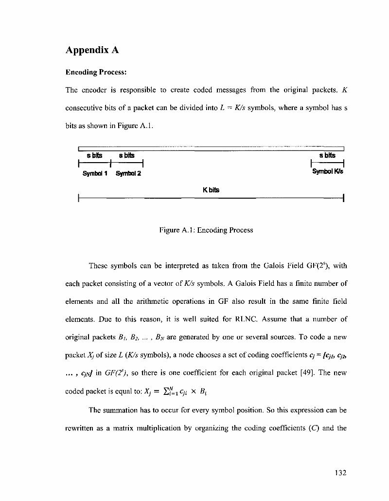
Appendix A
Encoding Process:
The encoder is responsible to create coded messages from the original packets. K
consecutive bits of a packet can be divided into L = K/s symbols, where a symbol has s
bits as shown in Figure A.l.
I — s bits s bits
I \— 1 Symbol 1 Symbol 2
Kbits
I —
Figure A. 1: Encoding Process
These symbols can be interpreted as taken from the Galois Field GF(2S), with
each packet consisting of a vector of K/s symbols. A Galois Field has a finite number of
elements and all the arithmetic operations in GF also result in the same finite field
elements. Due to this reason, it is well suited for RLNC. Assume that a number of
original packets Bi, B2, ... , BN are generated by one or several sources. To code a new
packet Xj of size L (K/s symbols), a node chooses a set of coding coefficients cy- = fcp, Cj2,
... , CjiyJ in GF(2S), so there is one coefficient for each original packet [49]. The new
coded packet is equal to: Xj = Y,i=i c]i x Bt
The summation has to occur for every symbol position. So this expression can be
rewritten as a matrix multiplication by organizing the coding coefficients (Q and the
sbits
h - 1 Symbol K/s
1
132
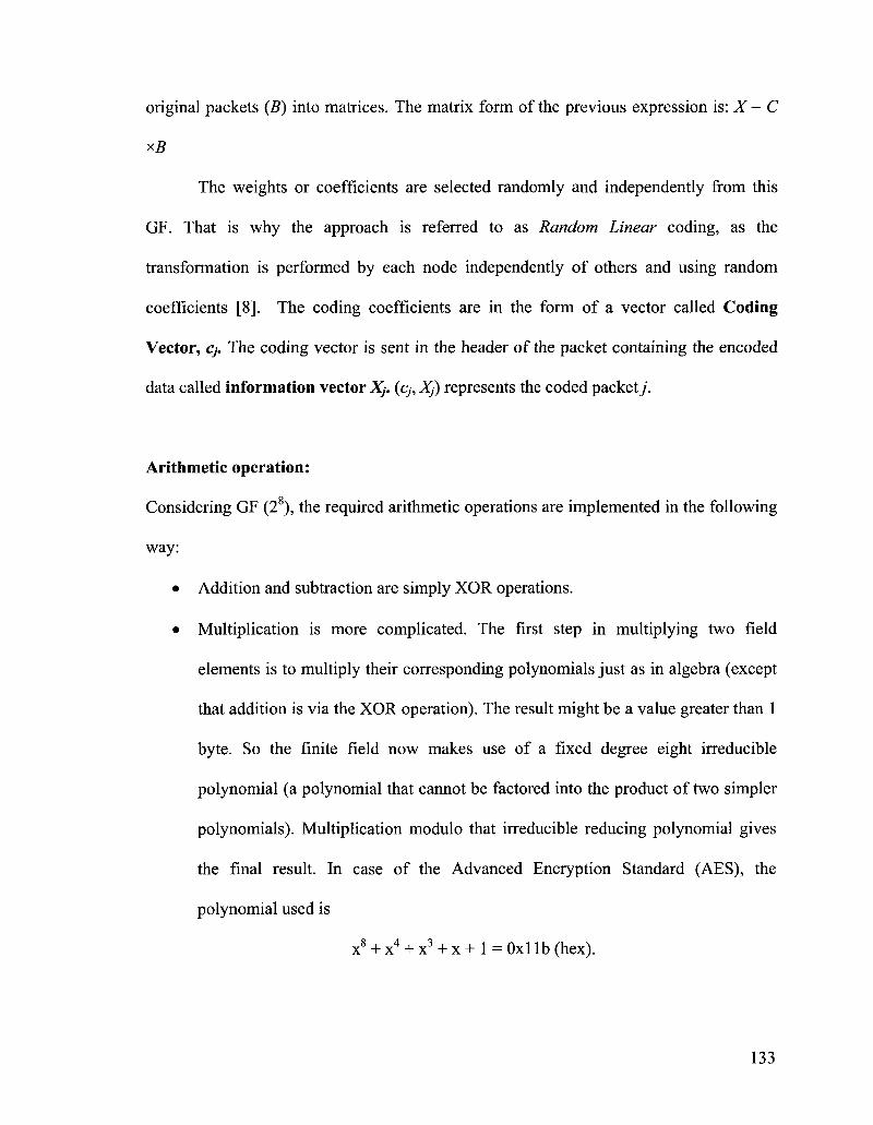
original packets (B) into matrices. The matrix form of the previous expression is: X = C
xB
The weights or coefficients are selected randomly and independently from this
GF. That is why the approach is referred to as Random Linear coding, as the
transformation is performed by each node independently of others and using random
coefficients [8]. The coding coefficients are in the form of a vector called Coding
Vector, Cj. The coding vector is sent in the header of the packet containing the encoded
data called information vector Xj. (9, Xj) represents the coded packety.
Arithmetic operation:
Considering GF (28), the required arithmetic operations are implemented in the following
way:
• Addition and subtraction are simply XOR operations.
• Multiplication is more complicated. The first step in multiplying two field
elements is to multiply their corresponding polynomials just as in algebra (except
that addition is via the XOR operation). The result might be a value greater than 1
byte. So the finite field now makes use of a fixed degree eight irreducible
polynomial (a polynomial that cannot be factored into the product of two simpler
polynomials). Multiplication modulo that irreducible reducing polynomial gives
the final result. In case of the Advanced Encryption Standard (AES), the
polynomial used is
x8 + x4 + x3 + x + 1 = Oxl lb (hex).
133
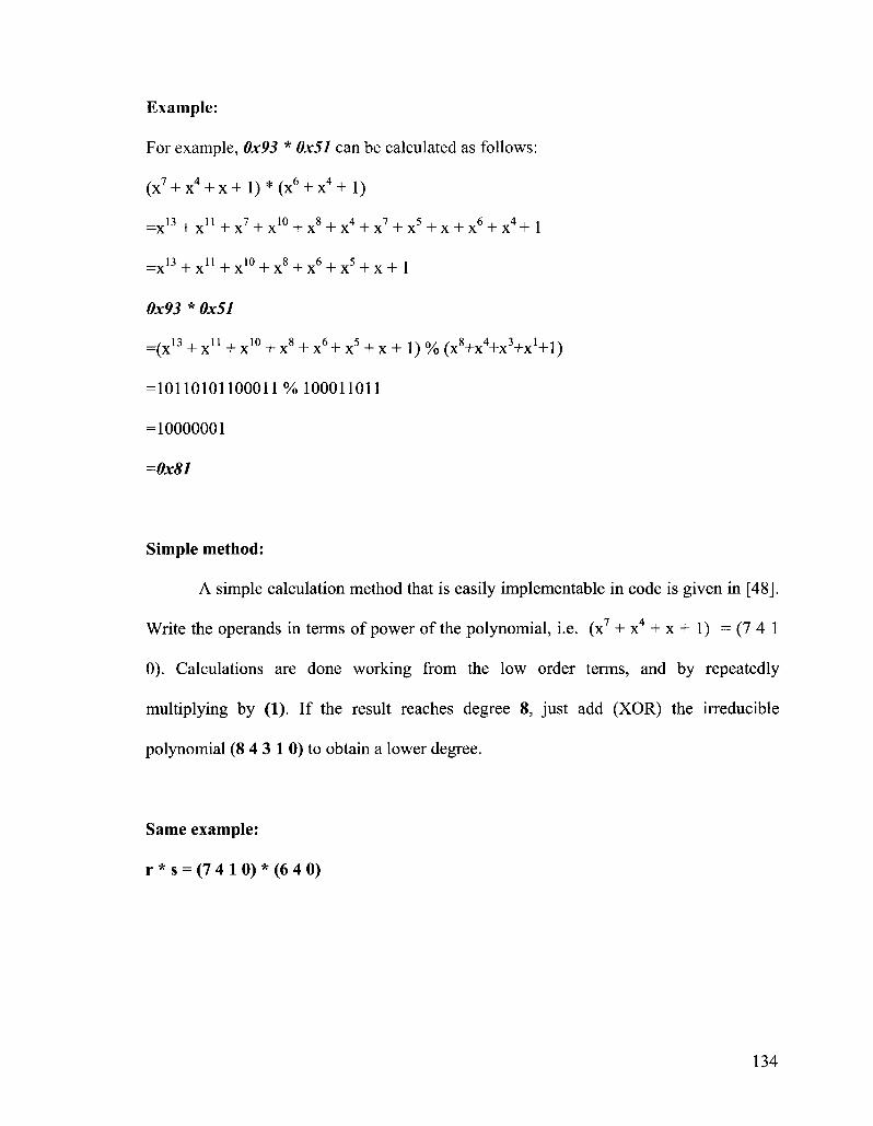
Example:
For example, 0x93 * 0x51 can be calculated as follows:
(x7 + x4 + x + l ) * ( x 6 + x 4 + l )
=x13 + x1 1+x7 + x10 + x8 + x4 + x7 + x X x + x6 + x 4 + l
=x13 + x u + x 1 0 + x8 + x6 + x X x + l
0x93 * 0x51
=(x13 + x1' + x10 + x8 + x6 + x5 + x + 1) % (x8+x4+x3+x'+l)
=10110101100011 % 100011011
=10000001
=0x81
Simple method:
A simple calculation method that is easily implementable in code is given in [48].
Write the operands in terms of power of the polynomial, i.e. (x7 + x4 + x + 1) = ( 7 4 1
0). Calculations are done working from the low order terms, and by repeatedly
multiplying by (1). If the result reaches degree 8, just add (XOR) the irreducible
polynomial (8 4 3 1 0) to obtain a lower degree.
Same example:
r * s = (7 4 1 0) * (6 4 0)
134

i
0
1
2
3
4
5
6
powers of r: r * (i)
(7 4 1 0 ) * (1) =
( 5432 0) * (1)
(6 5 4 3 1) *(1)
(7 6 5 4 2)*(1)
(7 65 4 10)* (1)
( 7 6 5 4 3 2 0)* (1)
Simplified Result
( 7 4 1 0 )
(8 5 2 1)
+(8 4 3 1 0)
( 5 4 3 2 10)
( 6 5 4 3 1)
(7 6 5 4 2)
( 8 7 6 5 3)
+(8 4 3 1 0)
( 7 6 5 4 10)
(8 7 65 2 1)
+(8 4 3 1 0)
( 7 6 5 4 3 2 0)
( 8 7 6 5 4 3 1)
+(8 4 3 10)
( 7 6 5 0)
Final Sum
(7 4 1 0 )
(7 4 1 0 )
+ ( 7 6 5 4 10)
( 6 5 )
( 6 5 )
+ (765 0)
(7 0) =
10000001
= 0x81
Table A.l: Simplified Multiplication on GF (2s)
Example for Encoding in RLNC:
Suppose we have 4 bytes (5, 6, 111, 152) to be encoded. We select 4*4=16 coding
coefficients as 4 coded packets are to be sent for the 4 symbols encoded together. The
135

example is provided using coding vector 3 to calculate the second coded symbol in the
encoded packet 3 (boxed values). The (randomly selected) coding vectors are as follows:
Coding vector 1:41, 35, 190, 132
Coding vector 2: 225, 108, 214, 174
Coding vector 3: |82, 144,73,241
Coding vector 4: 241, 187,233,235
The encoding is done as follows. Note that the operation here is over GF(28).
1st encoded byte: 41 * 5 + 35 * 6 + 190 * 111 + 132 * 152 = 209
2nd encoded byte: 225 * 5 + 108 * 6 + 214 * 111 + 174 * 152 = 40
3rd encoded byte: 82 * 5 + 144 * 6 + 73 * 111 +241 * 152=140
4th encoded byte: 241 * 5 + 187 * 6 + 233 * 111 + 235 * 152 = 195
Now we can form 4 packets, each consisting of a coding vector and the encoded byte,
with a size of 5 bytes:
Coding vector
r
Packet 1:41, 35,190,132, 209
Packet 2: 225,108, 214,174, 40
Packet 3: 82,144, 73, 241, 140
Packet 4: 241,187, 233, 235, 195
Coded symbol
Y=S
136
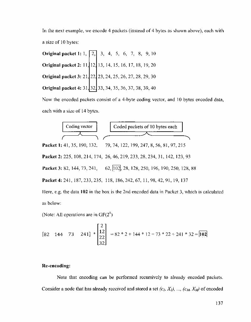
In the next example, we encode 4 packets (instead of 4 bytes as shown above), each with
a size of 10 bytes:
Original packet 1: 1
Original packet 2: 11
Original packet 3: 21
Original packet 4: 31 32
3, 4, 5, 6, 7, 8, 9, 10
12113, 14,15, 16,17,18,19,20
22 23, 24, 25, 26, 27, 28, 29, 30
33,34,35,36,37,38,39,40
Now the encoded packets consist of a 4-byte coding vector, and 10 bytes encoded data
each with a size of 14 bytes.
Coding vector Coded packets of 10 bytes each
( \ r X
Packet 1: 41, 35, 190, 132, 79, 74, 122, 199, 247, 8, 56, 81, 97, 215
Packet 2: 225, 108, 214, 174, 26, 46, 219, 233, 28, 234, 31, 142, 123, 93
Packet 3: 82, 144,73,241, 62, 102,28, 128,250, 196, 190,250, 128,88
Packet 4: 241, 187,233,235, 118, 186,242,67, 11,98,42,91,19, 137
Here, e.g. the data 102 in the box is the 2nd encoded data in Packet 3, which is calculated
as below:
(Note: All operations are in GF(28)
2
[82 144 73 241] * ^
32
82 * 2 + 144 * 12 + 73 * 22 + 241 * 32 = 102
Re-encoding:
Note that encoding can be performed recursively to already encoded packets.
Consider a node that has already received and stored a set (ci, Xj), ..., (CM, XM) of encoded
137

packets. This node may generate a new encoded packet (c, X) by picking a set of
coefficients h= [hi,..., hyl e GF(T) and computing the linear combination:
M
X^^hj.Xj
It is important that the corresponding encoding vector c is not simply equal to h,
since the coefficients are with respect to the original packets Bj, B2, ... , BN-
Straightforward algebra shows that the new coding vector is given by
M
c'i= l^hj.Cji
This operation may be repeated at several nodes in the network. Also note that it
is not necessary to decode a packet before applying this type of recursive encoding.
Decoding:
Assume a node has received the set (X Xj), ..., (CM, Xy) of encoded packets. In
order to retrieve the original packets, it needs to solve the system:
N
Xj = ^Cji.Bi
i=l
The Bi are the unknowns. This is a linear system with M equations and N
unknowns. We need M > N to have a chance of recovering all data, i.e., the number of
received packets needs to be at least as large as the number of original packets. This
linear system can also be given in a matrix form: B = C"1 x X
But the condition M >N is not sufficient, as some of the combinations might be linearly
dependent.
138
Decoding Process [8]:
Decoding requires solving a set of linear equations. A node stores the received
encoded packets as well as its own original packets row by row, into a so-called decoding
matrix. Initially this matrix is empty or it contains its own non-encoded packets with their
corresponding encoding vectors. When an encoded packet is received, it is inserted as the
last row into the decoding matrix. This matrix of coefficients is transformed into a
triangular matrix using standard Gaussian elimination (but all operations are performed
over the Galois Field). Only innovative packets are inserted. If a packet is non-innovative,
it is reduced to a row of Os by Gaussian elimination and is ignored.
139