1

Adaptive Primal-Dual Hybrid Gradient Methods forSaddle-Point Problems

Tom Goldstein, Min Li, Xiaoming Yuan, Ernie Esser, Richard Baraniuk

Abstract—The Primal-Dual hybrid gradient (PDHG) methodis a powerful optimization scheme that breaks complex problemsinto simple sub-steps. Unfortunately, PDHG methods require theuser to choose stepsize parameters, and the speed of convergenceis highly sensitive to this choice. We introduce new adaptivePDHG schemes that automatically tune the stepsize parametersfor fast convergence without user inputs. We prove rigorousconvergence results for our methods, and identify the conditionsrequired for convergence. We also develop practical implemen-tations of adaptive schemes that formally satisfy the convergencerequirements. Numerical experiments show that adaptive PDHGmethods have advantages over non-adaptive implementations interms of both efficiency and simplicity for the user.

I. INTRODUCTION

This manuscript considers saddle-point problems of form

minx∈X

maxy∈Y

f(x) + yTAx− g(y) (1)

where f and g are convex functions, A ∈ RM×N is a matrix,and X ⊂ RN and Y ⊂ RM are convex sets.

The formulation (1) is particularly appropriate for solvinginverse problems involving the `1 norm. Such problems takethe form

minx|Sx|+ µ

2‖Bx− f‖2 (2)

where | · | denotes the `1 norm, B and S are linear operators,and ‖ · ‖ is the `2 norm. The formulation (2) is useful becauseit naturally enforces sparsity of Sx. Many different problemscan be addressed by choosing different values for the sparsitytransform S.

In the context of image processing, S is frequently thegradient operator. In this case the `1 term becomes |∇u|,the total variation semi-norm [1]. Problems of this form arisewhenever an image is recovered from incomplete or noise-contaminated data. In this case, B is often a Gaussian blurmatrix or a sub-sampled fast transform, such as a Fourier orHadamard transform.

As we will see below, the problem (2) can be put in the“saddle-point” form (1) and can then be addressed using thetechniques described below. Many other common minimiza-tion problems can also be put in this common form, includingimage segmentation, TVL1 minimization, and general linearprograming.

In many problems of practical interest, f and g do not sharecommon properties, making it difficult to derive numericalschemes for (1) that address both terms simultaneously. How-ever, it frequently occurs in practice that efficient algorithmsexist for minimizing f and g independently. In this case, thePrimal-Dual Hybrid Gradient (PDHG) [2], [3] method is quite

useful. This method removes the coupling between f andg, enabling each term to be addressed separately. Because itdecouples f and g, the steps of PDHG can often be writtenexplicitly, as opposed to other splitting methods that requireexpensive minimization sub-problems.

One of the primary difficulties with PDHG is that it relieson step-size parameters that must be carefully chosen by theuser. The speed of the method depends heavily on the choiceof these parameters, and there is often no intuitive way tochoose them. Furthermore, the stepsize restriction for thesemethods depends on the spectral properties of A, which maybe unknown for general problems.

We will present practical adaptive schemes that optimizethe PDHG parameters automatically as the problem is solved.Our new methods are not only much easier to use in practice,but also result in much faster convergence than constant-stepsize schemes. After introducing the adaptive methods, weprove new theoretical results that guarantee convergence ofPDHG under very general circumstances, including adaptivestepsizes.

A. Notation

Given two vectors u, v ∈ RN , we will denote their discreteinner product by uT v =

∑i uivi. When u, v ∈ RΩ are not

column vectors, we will also use the “dot” notation for theinner product, u · v =

∑i∈Ω uivi.

The formulation (1) can be generalized to handle complex-valued vectors. In this case, we will consider the real part ofthe inner product. We use the notion <· to denote the realpart of a vector or scalar.

We will make use of a variety of norms, including the `2-norm, ‖u‖ =

√∑i u

2i , and the `1-norm, |u| =

∑i |ui|.

When M is a symmetric positive definite matrix, we definethe M -norm by

‖u‖2M = uTMu.

If M is indefinite, this does not define a proper norm. In thiscase, we will still write ‖u‖2M to denote the quantity uTMu,even though this is an abuse of notation.

For a matrix M, we can also define the “operator norm”

‖M‖op = maxu

‖Mu‖‖u‖

.

If M is symmetric, then the operator norm is the spectralradius of M, which we denote by ρ(M).

We use the notation ∂f to denote the sub-differential (i.e.,generalized derivative) of a function f .

arX

iv:1

305.

0546

v2 [

mat

h.N

A]

24

Mar

201

5

2

Finally, we will use χC to denote the characteristic functionof a convex set C, which is defined as follows:

χC(x) =

0, if x ∈ C∞, otherwise.

II. THE PRIMAL-DUAL HYBRID GRADIENT METHOD

The PDHG scheme has its roots in the well-known Arrow-Hurwicz scheme, which was originally proposed in the field ofeconomics and later refined for solving saddle point problemsby Popov [4]. While the simple structure of the Arrow-Hurwicz method made it appealing, tight stepsize restrictionsand poor performance make this method impractical for manyproblems.

Research in this direction was reinvigorated by the intro-duction of PDHG, which converges rapidly for a wide rangeof stepsizes. PDHG originally appeared in a technical reportby Zhu and Chan [5]. It was later analyzed for convergencein [2], [3], and studied in the context of image segmentationin [6]. An extensive technical study of the method and itsvariants is given by He and Yuan [7]. Several extensions ofPDHG, including simplified iterations for the case that f or gis differentiable, are presented by Condat [8].

PDHG is listed in Algorithm 1. The algorithm is inspiredby the forward-backward algorithm, as the primal and dualparameters are updated using a combination of forward andbackward steps. In steps (2-3), the method updates x todecreases the energy (1) by first taking a gradient descent stepwith respect to the inner product term in (1), and then takinga “backward” or proximal step involving f . In steps (5-6), theenergy (1) is increased by first marching up the gradient ofthe inner product term with respect to y, and then a backwardstep is taken with respect to g.

Require: x0 ∈ RN , y0 ∈ RM , σk, τk > 01: while Not Converged do2: xk+1 = xk − τkAT yk3: xk+1 = arg minx∈X f(x) + 1

2τk‖x− xk+1‖2

4: xk+1 = xk+1 + (xk+1 − xk)5: yk+1 = yk + σkAxk+1

6: yk+1 = arg miny∈Y g(y) + 12σk‖y − yk+1‖2

7: end whileAlgorithm 1: Basic PDHG

Note that steps 3 and 6 of Algorithm 1 require minimiza-tions. These minimization steps can be written in a morecompact form using the proximal operators of f and g:

JτF (x) = arg minx∈X

f(x) +1

2τ‖x− x‖2 = (I + τF )−1x

JσG(y) = arg miny∈Y

g(y) +1

2σ‖y − y‖2 = (I + σG)−1y.

(3)

Algorithm 1 has been analyzed in the case of constantstepsizes, τk = τ and σk = σ. In particular, it is known to con-verge as long as στ < 1

ρ(ATA)[2], [3], [7]. However, PDHG

typically does not converge when non-constant stepsizes areused, even in the case that σkτk < 1

ρ(ATA).

In this article, we identify the specific stepsize conditionsthat guarantee convergence and propose practical adaptivemethods that enforce these conditions.

Remark 1: Step 4 of Algorithm 1 is a prediction step of theform xk+1 = xk+1 + θ(xk+1 − xk), where θ = 1. Note thatPDHG methods have been analyzed for θ ∈ [−1, 1] (see [7]).Some authors have even suggested non-constant values of θas a means of accelerating the method [3]. However, the caseθ = 1 has been used almost exclusively in applications.

A. Optimality Conditions and Residuals

Problem (1) can be written in its unconstrained form usingthe characteristic functions for the sets X and Y . We have

minx∈RN

maxy∈RM

f(x) + χX(x) + yTAx− g(y)− χY (y). (4)

Let F = ∂f + χX(x), and G = ∂g + χY (y)1. From theequivalence between (1) and (4), we see that the optimalityconditions for (1) are

0 ∈ F (x?) +AT y? (5)0 ∈ G(y?)−A(x?). (6)

The optimality conditions (5,6) state that the derivative withrespect to both the primal and dual variables must be zero.This motivates us to define the primal and dual residuals

P (x, y) = F (x) +AT y

D(x, y) = G(y)−Ax.(7)

We can measure convergence of the algorithm by tracking thesize of these residuals. Note that the residuals are in generalmulti-valued (because they depend on the subdifferentials of fand g, as well as the characteristic functions of X and Y ). Wecan obtain explicit formulas for these residuals by observingthe optimality conditions for step 2 and 4 of Algorithm 1:

0 ∈ F (xk+1) +AT yk +1

τk(xk+1 − xk) (8)

0 ∈ G(yk+1)−A(2xk+1 − xk) +1

σk(yk+1 − yk). (9)

Manipulating these optimality conditions yields

Pk+1 =1

τk(xk − xk+1)−AT (yk − yk+1) (10)

∈ F (xk+1) +AT yk+1, (11)

Dk+1 =1

σk(yk − yk+1)−A(xk − xk+1) (12)

∈ G(yk+1)−Axk+1. (13)

Formulas (11) and (13) define a sequence of primal anddual residual vectors such that Pk ∈ P (xk, yk) and Dk ∈D(xk, yk).

We say that Algorithm 1 converges if

limk→∞

‖Pk‖2 + ‖Dk‖2 = 0.

1Note that ∂f + χX(x) = ∂f + ∂χX(x) precisely when the resolventminimizations (3) are feasible (see Rockafellar [9] Theorem 23.8), and in thiscase the optimality conditions (4) admit a solution. We will assume for theremainder of this article that the problem (4) is feasible.

3

Note that studying the residual convergence of Algorithm 1 ismore general than studying the convergence of subsequencesof iterates, because the solution to (1) need not be unique.

III. COMMON SADDLE-POINT PROBLEMS

Many common variational problems have saddle-point for-mulations that are efficiently solved using PDHG. While theapplications of saddle-point problems are vast, we focus hereon several simple problems that commonly appear in imageprocessing.

A. Total-Variation Denoising

A ubiquitous problem in image processing is minimizingthe Rudin-Osher-Fatemi (ROF) denoising model [1]:

minx|∇x|+ µ

2‖x− f‖2. (14)

The energy (14) contains two terms. The `2 term on the rightminimizes the squared error between the recovered image andthe noise-contaminated measurements, f . The TV term, |∇x|,enforces that the recovered image be smooth in the sense thatits gradient has sparse support.

The problem(14) can be formulated as a saddle-point prob-lem by writing the TV term as a maximization over the “dual”variable y ∈ R2×N , where the image x ∈ RN has N pixels:

TV (x) = |∇x| = max‖y‖∞≤1

y · ∇x. (15)

Note that the maximization is taken over the set

C∞ = y ∈ R2×N | y21,i + y2

2,i ≤ 1.

The TV-regularized problem (14) can then be written in itsprimal-dual form

maxy∈C∞

minx

µ

2‖x− f‖2 + y · ∇x (16)

which is clearly a saddle-point problem in the form (1) withf = µ

2 ‖x− f‖2, A = ∇, g = 0, X = RN , and Y = C∞.

To apply Algorithm 1, we need efficient solutions to thesub-problems in steps 3 and 6, which can be written

JτF (x) = arg minx

µ

2‖x− f‖2 +

1

2τ‖x− x‖2 (17)

=τ

τµ+ 1(µf +

1

τx) (18)

JσG(y) = arg miny∈C∞

1

2σ‖y − y‖2 =

(yi

maxyi, 1

)Mi=1

. (19)

B. TVL1

Another common denoising model is TVL1 [10]. Thismodel solves

minx|∇x|+ µ|x− f | (20)

which is similar to (14), except that the data term relies onthe `1 norm instead of `2. This model is very effective forproblems involving “heavy-tailed” noise, such as shot noiseor salt-and-pepper noise.

To put the energy (20) into the form (1), we write the dataterm in its variational form

µ|x− f | = maxy∈Cµ

yT (x− f)

where Cµ = y ∈ RN | |yi| ≤ µ.The energy (20) can then be minimized using the formula-

tionmax

y1∈C∞, y2∈Cµminxy1 · ∇x+ yT2 x− yT2 f (21)

which is of the form (1).

C. Globally Convex Segmentation

Image segmentation is the task of grouping pixels togetherby intensity and spatial location. One of the simplest modelsfor image segmentation is the globally convex segmentationmodel of Chan, Esedoglu, and Nikolova (CEN) [11], [12].Given an image f and two real numbers c1 and c2 we wishto partition the pixels into two groups depending on whethertheir intensity lies closer to c1 or c2. Simultaneously, we wantthe regions to have smooth boundaries.

The CEN segmentation model has the variational form

min0≤x≤1

|∇x|+ xT l (22)

where li = (fi− c1)2− (fi− c2)2. The inner-product term ofthe right forces the entries in x toward either 1 or 0, dependingon whether the corresponding pixel intensity in f is closer toc1 or c2. At the same time, the TV term enforces that theboundary is smooth.

Using the identity (15), we can write the model (22) as

maxy∈C∞

minx∈[0,1]

y · ∇x+ xT l. (23)

We can then apply Algorithm 1, where step 3 takes the form

JτF (x) = max0,minx, 1

and step 6 is given by (19).Generalizations of (22) to multi-label segmentations and

general convex regularizers have been presented in [13], [14],[15], [16]. Many of these models result in minimizationssimilar to (22), and PDHG methods have become a popularscheme for solving these models.

D. Compressed Sensing / Single-Pixel Cameras

In compressed sensing, one is interested in reconstructingimages from incomplete measurements taken in an orthogonaltransform domain (such as the Fourier or Hadamard domain).It has been shown that high-resolution images can be obtainedfrom incomplete data as long as the image has a sparserepresentation [17], [18], for example a sparse gradient.

The Single Pixel Camera (SPC) is an imaging modality thatleverages compressed sensing to reconstruct images using asmall number of measurements [19]. Rather than measuringin the pixel domain like conventional cameras, SPC’s measurea subset of the Hadamard transform coefficients of an image.

To reconstruct images, SPC’s rely on variational problemsof the form

minx|∇x|+ µ

2‖RHx− b‖2 (24)

4

where b contains the measured transform coefficients of theimage, and H is an orthogonal transform matrix (such as theHadamard transform). Here, R is a diagonal “row selector”matrix, with diagonal elements equal to 1 if the correspondingHadamard row has been measured, and 0 if it has not.

This problem can be put into the saddle-point form

maxy∈C∞

minx

µ

2‖RHx− b‖2 + y · ∇x

and then solved using PDHG.The solution to step 6 of Algorithm 1 is given by (19). Step

3 requires we solve

minx

µ

2‖RHx− b‖2 +

1

2τ‖x− x‖2.

Because H is orthogonal, we can write the solution to thisproblem explicitly as

x = HT

(µR+

1

τI

)−1

H

(µHTRb+

1

τx

).

Note that for compressed sensing problems of the form (24),PDHG has the advantage that all steps of the method can bewritten explicitly, and no expensive minimization sub-stepsare needed. This approach to solving (24) generalizes to anyproblem involving a sub-sampled orthogonal transform. Forexample, the Hadamard transform H could easily be replacedby a Fourier transform matrix.

E. `∞ Minimization

In wireless communications, one is often interested infinding signal representations with low peak-to-average powerratio (PAPR) [20], [21]. Given a signal z with high dynamicrange, we can obtain a more efficient representation by solving

minx‖x‖∞ subject to ‖Dx− z‖ ≤ ε (25)

where x is the new representation, D is the representationbasis, and ε is the desired level of representation accuracy [21].Minimizations of the form (25) also arise in numerous otherapplications, including robotics [22] and nearest neighborsearch [23].

The problem (25) can be written in the constrained form

minx1∈RN ,x2∈Cε

‖x1‖∞ subject to x2 = Dx1 − z

where Cε = z | ‖z‖ < ε. When we introduce Lagrangemultipliers y to enforce the equality constraint, we arrive atthe saddle-point formulation

maxy∈RM

minx1∈RN ,x2∈Cε

‖x1‖∞ + yT (Dx1 − x2 − z)

which is of the form (1).It often happens that D is a complex-valued frame (such as

a sub-sampled Fourier matrix). In this case, x and y can takeon complex values. The appropriate saddle-point problem isthen

maxy∈RM

minx1∈RN ,x2∈Cε

‖x1‖∞ + <yT (Dx1 − x2 − z)

and we can apply PDHG just as we did for real-valued prob-lems provided we are careful to use the Hermitian definition

of the matrix transpose (see the remark at the end of SectionV-B).

To apply PDHG to this problem, we need to evaluate theproximal minimization

minx‖x‖∞ +

1

2t‖x− x‖2

which can be computed efficiently using a sorting algorithm[24].

F. Linear Programming

Suppose we wish to solve a large-scale linear program inthe canonical form

minx

cTx

subject to Ax ≤ b, x ≥ 0(26)

where c and b are vectors, and A is a matrix [25]. This problemcan be written in the primal-dual form

maxy≥0

minx≥0

cTx+ yT (Ax− b)

where y can be interpreted as Lagrange multipliers enforcingthe condition Ax ≤ b [25].

Steps 3 and 6 of Algorithm 1 are now simply

JτF (x) = maxx− τc, 0,JσG(y) = maxy − σb, 0.

The PDHG solution to linear programs is advantageousfor some extremely large problems for which conventionalsimplex and interior-point solvers are intractable. Primal-dualsolvers for (26) have been studied in [26], and compared toconventional solvers. It has been observed that this approachis not efficient for general linear programming, however itbehaves quite well for certain structured programs, such asthose that arise in image processing [26].

IV. RESIDUAL BALANCING

When choosing the stepsize for PDHG, there is a tradeoffbetween the primal and dual residuals. Choosing a large valueof τk creates a very powerful minimization step in the primalvariables and a slow maximization step in the dual variables,resulting in very small primal residuals at the cost of large dualresiduals. Choosing τk to be small, on the other hand, resultsin small dual residuals at the cost of large primal errors.

Ideally, one would like to choose stepsizes so that the largerof Pk and Dk is as small as possible. If we assume theprimal/dual residuals decrease/increase monotonically with τk,then maxPk, Dk is minimized when both residuals are equalin magnitude. This suggests that τk be chosen to “balance” theprimal and dual residual – i.e., the primal and dual residualsshould be roughly the same size, up to some scaling to accountfor units. This principle has been suggested for other iterativemethods (see [27], [28]).

The particular residual balancing principle we suggest is toenforce

|Pk| ≈ s|Dk| (27)

5

where | · | denotes the `1 norm, and s is a scaling parameter.Residual balancing methods work by “tuning” parameters aftereach iteration to approximately maintain this equality. If theprimal residual grows disproportionately large, τk is increasedand σk is decreased (or vice-versa).

In (27) we use the `1-norm to measure the size of theresiduals. In principle, `1 could easily be replaced with the`2 norm, or any other norm. We have found that the `1 normperforms somewhat better than the `2 norm for some problems,because it is less sensitive to outliers that may dominate theresidual.

Note the proportionality in (27) depends on a constant s.This is to account for the effect of scaling the inputs (i.e.,changing units). For example, in the TVL1 model (20) theinput image f could be scaled with pixel intensities in [0, 1] or[0, 255]. As long as the primal step sizes used with the latterscaling are 255 times that of the former (and the dual stepsizes are 255 times smaller) both problems produce similarsequences of iterates. However, in the [0, 255] case the dualresiduals are 255 times larger than in the [0, 1] case while theprimal residuals are the same.

For image processing problems, we recommend using the[0, 255] scaling with s = 1, or equivalently the [0, 1] scalingwith s = 255. This scaling enforces that the saddle pointobjective (1) is nearly maximized with respect to y and thatthe saddle point term (15) is a good approximation of the totalvariation semi-norm.

V. ADAPTIVE METHODS

In this section, we develop new adaptive PDHG methods.The first method assumes we have a bound on ρ(ATA). Inthis case, we can enforce the stability condition

τkσk < L < ρ(ATA)−1. (28)

This is the same stability condition that guarantees conver-gence in the non-adaptive case. In the adaptive case, thiscondition alone is not sufficient for convergence but leads torelatively simple methods.

The second method does not require any knowledge ofρ(ATA). Rather, we use a backtracking scheme to gauranteeconvergence. This is similar to the Armijo-type backtrackingline searches that are used in conventional convex optimiza-tion. In addition to requiring no knowledge of ρ(ATA),the backtracking scheme has the advantage that it can userelatively long steps that violate the stability condition (28).Especially for problems with highly sparse solutions, this canlead to faster convergence than methods that enforce (28).

Both of these methods have strong convergence guarantees.In particular, we show in Section VI that both methodsconverge in the sense that the norm of the residuals goes tozero.

A. Adaptive PDHG

The first adaptive method is listed in Algorithm 2. The loopin Algorithm 2 begins by performing a standard PDHG stepusing the current stepsizes. In steps 4 and 5, we compute theprimal and dual residuals and store their `1 norms in pk and

dk. If the primal residual is sufficiently large compared to thedual residual then the primal stepsize is increased by a factorof (1− αk)−1, and the dual stepsize is decreased by a factorof (1 − αk). If the primal residual is somewhat smaller thanthe dual residual then the primal stepsize is decreased and thedual stepsize is increased. If both residuals are comparable insize, then the stepsizes remain the same on the next iteration.

The parameter ∆ > 1 is used to compare the sizes of theprimal and dual residuals. The stepsizes are only updated ifthe residuals differ by a factor greater than ∆.

The sequence αk controls the adaptivity level of themethod. We start with some α0 ∈ (0, 1). Every time we chooseto update the stepsize parameters, we define αk+1 = ηαk forsome η < 1. In this way, the adaptivity decreases over time.We will show in Section VI that this definition of αk isneeded to guarantee convergence of the method.

Remark 2: The adaptive scheme requires several arbitraryconstants as inputs. These are fairly easy to choose in practice.A fairly robust choice is a0 = 0.5, ∆ = 1.5, η = 0.95,and τ0 = σ0 = 1/

√ρ(ATA). However, these parameters can

certainly be tuned for various applications. As stated above,we recommend choosing s = 1 for imaging problems whenpixels lie in [0, 255], and s = 255 when pixels lie in [0, 1].

Remark 3: The computation of the residuals in steps 4and 5 of Algorithm 2 requires multiplications by AT and A,which seems at first to increase the cost of each iteration.Note however that the values of AT yk and Axk are alreadycomputed in the other steps of the algorithm. If we simply notethat AT (yk − yk+1) = AT yk −AT yk+1 and A(xk −xk+1) =Axk − Axk+1, then we can evaluate the residuals in steps 4and 5 without any additional multiplications by A or AT .

B. Backtracking PDHG

A simple modification of Algorithm 2 allows the methodto be applied when bounds on ρ(ATA) are unavailable, orwhen the stability condition (28) is overly conservative. Thisis accomplished by choosing “large” initial stepsizes, andthen decreasing the stepsizes using the “backtracking” schemedescribed below.

We will see in Section VI that convergence is guaranteed ifthe following “backtracking” condition holds at each step:

bk =2τkσk(yk+1 − yk)TA(xk+1 − xk)

γσk‖xk+1 − xk‖2 + γτk‖yk+1 − yk‖2≤ 1. (29)

where γ ∈ (0, 1) is a constant. If this inequality does not hold,then the stepsizes are too large. In this case we decrease thestepsizes by choosing

τk+1 = β τk/bk, and σk+1 = β σk/bk, (30)

for some β ∈ (0, 1). We recommend choosing γ = 0.75 andβ = 0.95, although the method is convergent for any γ, β ∈(0, 1). Reasons for this particular update choice, are elaboratedin the Section VI-D.

We will show in Section VI that this backtracking stepcan only be activated a finite number of times. Furthermore,enforcing the condition (29) at each step is sufficient toguarantee convergence, provided that one of the spaces X orY is bounded.

6

Require: x0 ∈ RN , y0 ∈ RM , σ0τ0 < ρ(ATA)−1, (α0, η) ∈ (0, 1)2,∆ > 1, s > 01: while pk, dk > tolerance do2: xk+1 = JτkF (xk − τkAT yk) . Begin with normal PDHG3: yk+1 = JσkG(yk + σkA(2xk+1 − xk))4: pk+1 = |(xk − xk+1)/τk −AT (yk − yk+1)| . Compute primal residual5: dk+1 = |(yk − yk+1)/σk −A(xk − xk+1)| . Compute dual residual6: if pk+1 > sdk+1∆ then . If primal residual is large...7: τk+1 = τk/(1− αk) . Increase primal stepsize8: σk+1 = σk(1− αk) . Decrease dual stepsize9: αk+1 = αkη . Decrease adaptivity level

10: end if11: if pk+1 < sdk+1/∆ then . If dual residual is large...12: τk+1 = τk(1− αk) . Decrease primal stepsize13: σk+1 = σk/(1− αk) . Increase dual stepsize14: αk+1 = αkη . Decrease adaptivity level15: end if16: if sdk+1/∆ ≤ pk+1 ≤ sdk+1∆ then . If residuals are similar...17: τk+1 = τk . Leave primal step the same18: σk+1 = σk . Leave dual step the same19: αk+1 = αk . Leave adaptivity level the same20: end if21: end while

Algorithm 2: Adaptive PDHG

The initial stepsizes τ0 and σ0 should be chosen so thatτ0σ0 is somewhat larger than ρ(ATA)−1. In the numericalexperiments below, we choose

τ0 = σ0 =

√2‖xr‖‖ATAxr‖

(31)

where xr is a random Gaussian distributed vector. Note thatthe ratio ‖A

TAxr‖‖xr‖ is guaranteed to be less than ρ(ATA), and

thus τ0σ0 > ρ(ATA)−1. The factor of 2 is included to accountfor problems for which the method is stable with large steps.

Remark 4: Note that our convergence theorems requireeither X or Y to be bounded. This requirement is indeed satis-fied by most of the common saddle-point problems describedin Section III. However, we have found empirically that thescheme is quite stable even for unbounded X and Y . Forthe linear programming example, neither space is bounded.Nonetheless, the backtracking method converges reliably inpractice.

Remark 5: In the case of complex-valued problems, both xand y may take on complex values, and the relevant saddle-point problem is

minx∈X

maxy∈Y

f(x) + <yTAx − g(y)

where <· denotes the real part of a vector. In this casethe numerator of bk may have an imaginary component. Thealgorithm is still convergent as long as we replace bk with itsreal part and use the definition

bk =<

2τkσk(yk+1 − yk)TA(xk+1 − xk)

γσk‖xk+1 − xk‖2 + γτk‖yk+1 − yk‖2. (32)

VI. CONVERGENCE THEORY

A. Variational Inequality Formulation

For notational simplicity, we define the vector quantities

uk =

(xkyk

), R(u) =

(P (x, y)D(x, y)

), (33)

and the matrices

Mk =

(τ−1k I −AT−A σ−1

k I

), Hk =

(τ−1k I 00 σ−1

k I

),

Q(u) =

(AT y−Ax

).

(34)

This notation was first suggested to simplify PDHG by Heand Yuan [7].

Using this notation, it can be seen that the iterates of PDHGsatisfy

0 ∈ R(uk+1) +Mk(uk+1 − uk). (35)

Also, the optimality conditions (5) and (6) can be writtensuccinctly as

0 ∈ R(u?). (36)

Note that R is monotone (see [29]), meaning that

(u− u)T (R(u)−R(u)) ≥ 0, ∀u, u.

Following [7], it is also possible to formulate each step ofPDHG as a variational inequality (VI). If u? = (x?, y?) is asolution to (1), then x? minimizes (1) (for fixed y?) . Moreformally,

f(x)− f(x?) + (x− x?)TAT y? ≥ ∀x ∈ X. (37)

Likewise, (1) is maximized by y?, and so

− g(y) + g(y?) + (y − y?)TAx? ≤ 0 ∀ y ∈ Y. (38)

7

Subtracting (38) from (37) yields the VI formulation

φ(u)− φ(u?) + (u− u?)TQ(u?) ≥ 0 ∀u ∈ Ω. (39)

where φ(u) = f(x) + g(y) and Ω = X × Y. We say that apoint u is an approximate solution to (1) with VI accuracy εif

φ(u)− φ(u) + (u− u)TQ(u) ≥ −ε ∀u ∈ B1(u) ∩ Ω

where B1(u) is a unit ball centered at u.In Section VI-G, we prove two convergence results for

adaptive PDHG. First we prove the residuals vanish as k →∞.Next, we prove a O(1/k) ergodic convergence rate using theVI notion of convergence.

B. Stepsize Conditions

We now discuss conditions that guarantee convergence ofadaptive PDHG. We delay the formal convergence proofs untilSection VI-C. We begin by defining the following constants:

δk = min

τk+1

τk,σk+1

σk, 1

φk = 1− δk = max

τk − τk+1

τk,σk − σk+1

σk, 0

. (40)

The constant δ quantifies the stepsize change, and φ quantifiesthe relative decrease in the stepsizes between iterations.

Consider the following conditions on the step-sizes inAlgorithm 1.

Two conditions must always hold to guarantee convergence:(A) The stepsizes must remain bounded, and (B) the sequenceφi must be summable. Together, these conditions ensure thatthe steps sizes do not oscillate too wildly as k gets large.

In addition, either C1 or C2 must hold. When we knowthe spectral radius of ATA, we can use condition C1 toenforce that the method is stable. When we have no knowledgeof ρ(ATA), or when we want to take large stepsizes, thebacktracking condition C2 can also be used to enforce stability.We will see that for small enough stepsizes, this backtrackingcondition can always be satisfied.

Note that condition C1 is slightly stronger than conditionC2. The advantage of condition C1 is that it results issomewhat simpler methods because backtracking does notneed to be used. However when backtracking is used to enforcecondition C2, we can take larger steps that violate conditionC1.

In the following sub-sections, we explain how Algorithm 2and its backtracking variant explicitly satisfy conditions A, B,and C, and are therefore guaranteed to converge. In SectionVI-C, we prove convergence of the general Algorithm 1 underassumptions A, B, and C.

C. Convergence of the Adaptive Method

Algorithm 2 is a practical implementation of adaptivePDHG that satisfies conditions A, B, and C1. An examinationof Algorithm 2 reveals that there are three possible stepsizeupdates depending on the balance between the residuals.Regardless of which update occurs, the product τkσk remains

unchanged at each iteration, and so τkσk = τ0σ0 = L <ρ(ATA)−1. It follows that condition A and C1 are satisfied.

Also, because 0 < αk < 1, we have

φk = 1−min

τk+1

τk,σk+1

σk, 1

=

αk, if the steps are updated1, otherwise.

(41)

Note that every time we change the stepsizes, we updateαk+1 = ηαk where η < 1. Thus the non-zero entries inthe sequence φk form a decreasing geometric sequence. Itfollows that the summation condition B is satisfied.

Because Algorithm 2 satisfies conditions A , B and C, itsconvergence is guaranteed by the theory presented in SectionVI-C.

D. Convergence of the Backtracking Method

As we shall prove in Section VI-C, the backtracking step istriggered only a finite number of times. Thus, the backtrackingmethod satisfies conditions A and B.

We can expand condition C2 using the definition of ‖ · ‖Mk

and ‖ · ‖Hk to obtain

1

τk‖xk+1 − xk‖2+

1

σk‖yk+1 − yk‖2

− 2(yk+1 − yk)TA(xk+1 − xk)

>c

τk‖xk+1 − xk‖2 +

c

σk‖yk+1 − yk‖2.

If we combine like terms and let γ = 1−c, then this conditionis equivalent to

γ

τk‖xk+1−xk‖2 +

γ

σk‖yk+1 − yk‖2 (42)

> 2(yk+1 − yk)TA(xk+1 − xk). (43)

If we note that the left side of (42) is non-negative, then wecan easily see that this condition is equivalent to (29). Thus,the backtracking conditions (29) explicitly enforce conditionC2, and the convergence of Algorithm 2 with backtracking isguaranteed by the analysis below.

We now address the form of the backtracking update (30). Asimple Armijo-type backtracking scheme would simply chooseτk+1 = ξkτk and σk+1 = ξσk, where ξ < 0, every time that(42) is violated. However if our initial guess for L is very large,then this backtracking scheme could be very slow. Rather, wewish to predict the value of ξ that makes (42) hold. To do this,we assume (as a hueristic) that the values of ‖xk+1−xk‖ and‖yk+1− yk‖ decrease linearly with ξ. Under this assumption,the value of ξ that makes (42) into an equality is ξk = b−1

k .In order to guarantee that the stepsizes can become arbitrarilysmall, we make the slightly more conservative choice of ξk =β/bk for β < 1.

E. Sketch of Proof

The overall strategy of our convergence proof is to showthat the PDHG method satisfies a Fejer inequality, i.e., aninequality stating that the iterates move toward the solution

8

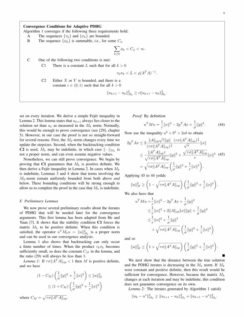
Convergence Conditions for Adaptive PDHGAlgorithm 1 converges if the following three requirements hold:

A The sequences τk and σk are bounded.B The sequence φk is summable, i.e., for some Cφ∑

k≥0

φk < Cφ <∞.

C One of the following two conditions is met:C1 There is a constant L such that for all k > 0

τkσk < L < ρ(ATA)−1.

C2 Either X or Y is bounded, and there is aconstant c ∈ (0, 1) such that for all k > 0

‖uk+1 − uk‖2Mk≥ c‖uk+1 − uk‖2Hk .

set on every iteration. We derive a simple Fejer inequality inLemma 2. This lemma states that uk+1 always lies closer to thesolution set than uk as measured in the Mk norm. Normally,this would be enough to prove convergence (see [29], chapter5). However, in our case the proof is not so straight-forwardfor several reasons. First, the Mk-norm changes every time weupdate the stepsizes. Second, when the backtracking conditionC2 is used, Mk may be indefinite, in which case ‖ · ‖Mk

isnot a proper norm, and can even assume negative values.

Nonetheless, we can still prove convergence. We begin byproving that C1 guarantees that Mk is positive definite. Wethen derive a Fejer inequality in Lemma 2. In cases when Mk

is indefinite, Lemmas 3 and 4 show that terms involving theMk-norm remain uniformly bounded from both above andbelow. These bounding conditions will be strong enough toallow us to complete the proof in the case that Mk is indefinite.

F. Preliminary Lemmas

We now prove several preliminary results about the iteratesof PDHG that will be needed later for the convergencearguments. This first lemma has been adapted from He andYuan [7]. It shows that the stability condition C1 forces thematrix Mk to be positive definite. When this condition issatisfied, the operator uTMku = ‖u‖2Mk

is a proper normand can be used in our convergence analysis.

Lemma 1 also shows that backtracking can only occura finite number of times. When the product τkσk becomessufficiently small, so does the constant CM in the lemma, andthe ratio (29) will always be less than 1.

Lemma 1: If τσ‖ATA‖op < 1 then M is positive definite,and we have

(1− CM )

(1

σ‖y‖2 +

1

τ‖x‖2

)≤ ‖u‖2M

≤ (1 + CM )

(1

σ‖y‖2 +

1

τ‖x‖2

)where CM =

√τσ‖ATA‖op.

Proof: By definition

uTMu =1

τ‖x‖2 − 2yTAx+

1

σ‖y‖2. (44)

Now use the inequality a2 + b2 > 2ab to obtain

2yTAx ≤ 2‖A‖op

√τ‖y‖

(τσ‖ATA‖op)14

(τσ‖ATA‖op)14

√τ

‖x‖

≤ ‖ATA‖opτ√τσ‖ATA‖op

‖y‖2 +

√τσ‖ATA‖op

τ‖x‖2

=√τσ‖ATA‖op

(1

σ‖y‖2 +

1

τ‖x‖2

).

(45)

Applying 45 to 44 yeilds

‖u‖2M ≥(

1−√τσ‖ATA‖op

)(1

σ‖y‖2 +

1

τ‖x‖2

).

We also have that

uTMu =1

τ‖x‖2 − 2yTAx+

1

σ‖y‖2

≤1

τ‖x‖2 + 2‖A‖op‖x‖‖y‖+

1

σ‖y‖2

≤1

τ‖x‖2 +

1

σ‖y‖2

+√τσ‖ATA‖op

(1

σ‖y‖2 +

1

τ‖x‖2

)and so

‖u‖2M ≤(

1 +√τσ‖ATA‖op

)(1

σ‖y‖2 +

1

τ‖x‖2

).

We next show that the distance between the true solutionand the PDHG iterates is decreasing in the Mk norm. If Mk

were constant and positive definite, then this result would besufficient for convergence. However, because the matrix Mk

changes at each iteration and may be indefinite, this conditiondoes not guarantee convergence on its own.

Lemma 2: The iterates generated by Algorithm 1 satisfy

‖uk − u?‖2Mk≥ ‖uk+1 − uk‖2Mk

+ ‖uk+1 − u?‖2Mk.

9

Proof: Subtracting (35) from (36) gives us

Mk(uk+1 − uk) ∈ R(u?)−R(uk+1).

Taking the inner product with (u? − uk+1) gives us

(u? − uk+1)TMk(uk+1 − uk)

≥ (u? − uk+1)T (R(u?)−R(uk+1)).

Because R is monotone, the right hand side of the aboveequation is non-negative, and so

(u? − uk+1)TMk(uk+1 − uk) ≥ 0. (46)

Now, observe the identity

‖uk − u?‖2Mk= ‖uk+1 − uk‖2Mk

+ ‖uk+1 − u?‖2Mk

+ 2(uk − uk+1)TMk(uk+1 − u?).

Applying (46) yields the result.We now show that the iterates generated by PDHG remain

bounded.Lemma 3: Suppose the step sizes for Algorithm 1 satisfy

conditions A, B and C. Then

‖uk − u?‖2Hk ≤ CUfor some upper bound CU > 0.

Proof: We first consider the case of condition C1. From(45) we have

2yTAx ≤√τσ‖ATA‖op

(1

σ‖y‖2 +

1

τ‖x‖2

).

Subtracting 2√τσ‖ATA‖opyTAx from both sides yields(

2− 2√τσ‖ATA‖op

)yTAx

≤√τσ‖ATA‖op

(1

σ‖y‖2 +

1

τ‖x‖2 − 2yTAx

)= ‖u‖2M

√τσ‖ATA‖op.

Taking x = xk+1 − x?, y = yk+1 − y?, τ = τk+1, andσ = σk+1, and noting that τk+1σk+1 < L we obtain

2(yk+1 − y?)TA(xk+1 − x?) ≤ C1‖uk+1 − u?‖2Mk+1

where C1 =

√L‖ATA‖op

1−√L‖ATA‖op

> 0.

Applying this to the result of Lemma 2, yields

‖uk − u?‖2Mk≥ ‖uk+1 − u?‖2Mk

=‖uk+1 − u?‖2Hk + (yk+1 − y?)TA(xk+1 − x?)≥δk‖uk+1 − u?‖2Hk+1

+ (yk+1 − y?)TA(xk+1 − x?)≥δk‖uk+1 − u?‖2Mk+1

+ (1− δk)(yk+1 − y?)TA(xk+1 − x?)≥δk‖uk+1 − u?‖2Mk+1

− (1− δk)C1‖uk+1 − u?‖2Mk+1

=(1− (1 + C1)φk)‖uk+1 − u?‖2Mk+1.

Note that (1+C1)φk > 1 for only finitely many k , and so weassume without loss of generality that k is sufficiently largethat (1− (1 + C1)φk) > 0. We can then write

‖u1 − u?‖2M1≥n−1∏k=1

(1− (1 + C1)φk)‖un − u?‖2Mn. (47)

Since∑k φk < ∞, we have that

∑k(1 + C1)φk < ∞, and

the product on the right of (47) is bounded away from zero.Thus, there is a constant C2 with

‖u1−u?‖2M1‖ ≥ C2‖un−u?‖2Mn

≥ C2(1−CM )‖un−u?‖2Hn

and the lemma is true in the case of assumption C1.We now consider the case where condition C2 holds. We

assume without loss of generality that Y is bounded (the caseof bounded X follows by nearly identical arguments). In thiscase, we have ‖y‖ ≤ Cy for all y ∈ Y.

Note that

‖uk+1−u?‖Mk+1= −(yk+1 − y?)TA(xk+1 − x?) (48)

+1

τk+1‖xk+1 − x?‖2 +

1

σk+1‖yk+1 − y?‖2

≥− 2Cy‖A‖op‖xk+1 − x?‖ (49)

+1

τk+1‖xk+1 − x?‖2 +

1

σk+1‖yk+1 − y?‖2. (50)

When ‖xk+1−x?‖ grows sufficiently large, the term involvingthe square of this norm dominates the value of (50). Sinceτk and σk are bounded from above, it follows that thereis some positive Cx such that whenever

1

τk+1‖xk+1 − x?‖2 +

1

σk+1‖yk+1 − y?‖2 ≥ Cx (51)

we have

1

τk+1‖xk+1 − x?‖2 +

1

σk+1‖yk+1 − y?‖2 (52)

≥ 4Cy‖A‖op‖xk+1 − x?‖. (53)

Combining (53) with (50) yields

2‖uk+1 − u?‖Mk+1≥ 1

τk+1‖xk+1 − x?‖2 (54)

+1

σk+1‖yk+1 − y?‖2 (55)

whenever (51) holds. In this case, we have

‖uk+1−u?‖2Mk= −(yk+1 − yk)TA(xk+1 − x?) (56)

+1

τk‖xk+1 − x?‖2 +

1

σk‖yk+1 − y?‖2

≥− (yk+1 − y?)TA(xk+1 − x?) (57)

+δkτk+1

‖xk+1 − x?‖2 +δkσk+1

‖yk+1 − y?‖2

=‖uk+1 − u?‖2Mk+1(58)

− φkτk+1

‖xk+1 − x?‖2 −φkσk+1

‖yk+1 − y?‖2

≥ (1− 2φk)‖uk+1 − u?‖2Mk+1. (59)

Applying (59) to Lemma 2, we see that

‖uk − u?‖2Mk≥ (1− 2φk)‖uk+1 − u?‖2Mk+1

. (60)

Note that limk→∞ φi = 0, and so we may assume withoutloss of generality that 1 − 2φk > 0 (this assumption is onlyviolated for finitely many k).

10

Now, consider the case that (51) does not hold. We have

‖uk+1−u?‖2Mk≥ ‖uk+1 − u?‖2Mk+1

− φkτk+1

‖xk+1 − x?‖2 −φkσk+1

‖yk+1 − y?‖2 (61)

≥‖uk+1 − u?‖2Mk+1− φkCx. (62)

Applying (62) to Lemma 2 yields

‖uk − u?‖2Mk≥ ‖uk+1 − u?‖2Mk+1

− φkCx. (63)

From (60) and (63), it follows by induction that

‖u0 − u?‖2M0≥∏i∈IC

(1− 2φi)‖uk+1 (64)

− u?‖2Mk+1−∑i

φiCx (65)

where IC = i | 1τk+1‖xk+1−x?‖2+ 1

σk+1‖yk+1−y?‖2 ≥ Cx.

Note again that we have assumed without loss of generalitythat k is large, and thus 1− 2φk > 0.

We can rearrange (64) to obtain

‖uk+1 − u?‖2Mk+1≤‖u0 − u?‖2M0

+ Cx∑i φi∏

i(1− 2φi)<∞

which shows that ‖uk − u?‖2Mkremains bounded.

Finally, note that since τk, σk, and ‖uk − u?‖Mkare

bounded from above, it follows from (50) that 1τk‖xk − x?‖2

is bounded from above. But 1σk‖yk − y?‖2 is also bounded

from above, and so ‖uk − u?‖Hk is bounded as well.Lemma 3 established upper bounds on the sequence of

iterates. To complete our convergence proof we also needlower bounds on ‖uk − u?‖2Mk

. Note that in the case ofindefinite Mk, this quantity may be negative. The followingresult show that ‖uk − u?‖2Mk

does not approach negativeinfinity.

Lemma 4: Suppose the step sizes for Algorithm 1 satisfyconditions A, B, and C. Then

‖uk+1 − u?‖2Mk≥ CL

for some lower bound CL.Proof: In the case that C1 holds, Lemma 1 tells us that

Mk is positive definite. In this case ‖ · ‖2Mkis a proper norm

and‖uk+1 − u?‖2Mk

≥ 0.

In the case that C2 holds, we have that either X or Y isbounded. Assume without loss of generality that Y is bounded.We then have ‖y‖ < Cy for all y ∈ Y . We can then obtain

‖uk+1 − u?‖2Mk≥ 1

τk‖xk+1 − x?‖2 (66)

− 2Cy‖A‖op‖xk+1 − x?‖+4C2

y

σk

≥ 1

minτk‖xk+1 − x?‖2 (67)

− 2Cy‖A‖op‖xk+1 − x?‖+4C2

y

minσk. (68)

Note that (68) is quadratic in ‖xk+1−x?‖, and so this quantityis bounded from below.

We now present one final lemma, which bounds a suminvolving the differences between adjacent iterates.

Lemma 5: Under conditions A, B, and C, we haven∑k=1

‖uk−u‖2Mk−‖uk−u‖2Mk−1

< CφCU +CφCH‖u−u?‖2

where CH is a constant such that ‖u−u?‖2Hk < CH‖u−u?‖2.Proof: We expand the summation on the left side of (70)

using the definition of Mk to obtainn∑k=1

‖uk − u‖2Mk− ‖uk − u‖2Mk−1

=

n∑k=1

(1

τk− 1

τk−1)‖xk − x‖2 + (

1

σk− 1

σk−1)‖yk − y‖2

≤n∑k=1

(1− δk−1)

(1

τk‖xk − x‖2 +

1

σk‖yk − y‖2

)=

n∑k=1

φk−1‖uk − u‖2Hk

≤n∑k=1

φk−1

(‖uk − u?‖2Hk + ‖u− u?‖2Hk

)≤

n∑k=1

φk−1

(CU + CH‖u− u?‖2

)≤ CφCU + CφCH‖u− u?‖2 <∞,

(69)

where we have used the bound ‖uk − u?‖2Hk < CU fromLemma 3.

G. Convergence TheoremsIn this section, we prove convergence of Algorithm 1 under

assumptions A, B, and C. The idea is to show that the normsof the residuals have a finite sum and thus converge to zero.Because the “natural” norm of the problem, the Mk-norm,changes after each iteration, we must be careful to bound thedifferences between the norms used at each iteration. For thispurpose, condition B will be useful because it guarantees thatthe various Mk-norms do not differ too much as k gets large.

Theorem 1: Suppose that the stepsizes in Algorithm 1 sat-isfy conditions A and B, and either C1 or C2. Then thealgorithm converges in the residuals, i.e.

limk→∞

‖Pk‖2 + ‖Dk‖2 = 0.

Proof:Rearranging Lemma (2) gives us

‖uk − u?‖2Mk− ‖uk+1 − u?‖2Mk

≥ ‖uk+1 − uk‖2Mk. (70)

Summing (70) for 1 ≤ k ≤ n gives usn∑k=1

‖uk+1−uk‖2Mk≤ ‖u1 − u?‖2M0

− ‖un+1 − u?‖2Mn

+

n∑k=1

‖uk − u?‖2Mk− ‖uk − u?‖2Mk−1

.

(71)

11

Applying Lemma 5 to (71), and noting from Lemma 4 that‖un+1 − u?‖Mn is bounded from below, we see that

n∑k=1

‖uk+1 − uk‖2Mk<∞.

It follows that limk→∞ ‖uk+1 − uk‖Mk= 0. If condition C2

holds, then this clearly implies that

limk→∞

‖uk+1 − uk‖Hk = 0. (72)

If condition C1 holds, then we still have (72) from Lemma 1.Since τk and σk are bounded from above, (72) implies that

limk→∞

‖uk+1 − uk‖ = 0. (73)

Recall the definition of Rk in equation (33). From (35), weknow that

Rk = Mk(uk − uk+1) ∈ R(uk+1),

and so

limk→∞

‖Rk‖ = limk→∞

‖M(uk+1 − uk)‖ (74)

≤ maxk‖Mk‖ lim

k→∞‖uk+1 − uk‖ = 0. (75)

Theorem 2: Suppose that the stepsizes in Algorithm 1 sat-isfy conditions A, B, and C. Consider the sequence definedby

ut =1

t

t∑k=1

uk.

This sequence satisfies the convergence bound

φ(u)− φ(ut) + (u− ut)TQ(ut) ≥‖u− ut‖2Mt

− ‖u− u0‖2M0− CφCU − CφCH‖u− u?‖2

2t.

Proof:We begin with the following identity (a special case of the

polar identity for normed vector spaces):

(u− uk+1)TMk(uk − uk+1) =1

2(‖u− uk+1‖2Mk

− ‖u− uk‖2Mk) +

1

2‖uk − uk+1‖2Mk

.

We apply this to the VI formulation of the PDHG iteration(39) to get

φ(u)− φ(uk+1) + (u− uk+1)TQ(uk+1)

≥ 1

2

(‖u− uk+1‖2Mk

− ‖u− uk‖2Mk

)+

1

2‖uk − uk+1‖2Mk

. (76)

Note that

(u− uk+1)TQ(u− uk+1) = (x− xk+1)AT (y − yk+1)

− (y − yk+1)A(x− xk+1) = 0, (77)

and so

(u− uk+1)TQ(u) = (u− uk+1)TQ(uk+1). (78)

Also, both conditions C1 and C2 guarantee that

‖uk − uk+1‖2Mk≥ 0.

These observations reduce (76) to

φ(u)− φ(uk+1) + (u− uk+1)TQ(u)

≥ 1

2

(‖u− uk+1‖2Mk

− ‖u− uk‖2Mk

). (79)

We now sum (79) for k = 0 to t− 1, and invoke Lemma 5.

2

t−1∑k=0

φ(u)− φ(uk+1) + (u− uk+1)TQ(u)

≥‖u− ut‖2Mt− ‖u− u0‖2M0

+

t∑k=1

(‖u− uk‖2Mk−1

− ‖u− uk‖2Mk

)≥‖u− ut‖2Mt

− ‖u− u0‖2M0

− CφCU − CφCH‖u− u?‖2.

(80)

Because φ is convex,

t−1∑k=0

φ(uk+1) ≤ tφ

(1

t

t∑k=1

uk

)= tφ(ut).

The left side of (80) therefore satisfies

2t(φ(u)− φ(ut) + (u− ut)TQ(u)

)≥ 2

t−1∑k=0

φ(u)− φ(uk+1) + (u− uk+1)TQ(u). (81)

Combining (80) and (81) yields the tasty bound

φ(u)− φ(ut) + (u− ut)TQ(u)

≥‖u− ut‖2Mt

− ‖u− u0‖2M0− CφCU − CφCH‖u− u?‖2

2t.

Applying (78) proves the theorem.Note that Lemma 3 guarantees uk remains bounded, and

thus ut is bounded also. Furthermore, because τk andσk remain bounded, the spectral radii of the matrices Mtremain bounded as well. It follows that, provided ‖u−ut‖ ≤ 1,there is a C with

‖u− u0‖2M0− ‖u− ut‖2Mt

≤ C ∀ t > 0, u ∈ B1(ut).

We then have

φ(u)− φ(ut) + (u− ut)TQ(ut)

≥ −C − CφCU − CφCH‖u− u?‖2

2t

and the algorithm converges with rate O(1/t) in an ergodicsense.

12

VII. NUMERICAL RESULTS

To demonstrate the performance of the new adaptive PDHGschemes, we apply them to the test problems described inSection III. We run the algorithms with parameters α0 = 0.5,∆ = 1.5, and η = 0.95. The backtracking method is run withγ = 0.75, β = 0.95, and we initialize stepsizes using formula(31). We terminate the algorithms when both the primal anddual residual norms (i.e. |Pk| and |Dk|) are smaller than 0.05,unless otherwise specified.

We consider four variants of PDHG. The method“Adapt:Backtrack” denotes Algorithm 2 with backtrackingadded. The initial stepsizes are chosen according to (31).The method “Adapt: τσ = L” refers to the adaptive methodwithout backtracking with τ0 = σ0 = 0.95ρ(ATA)−

12 .

We also consider the non-adaptive PDHG with two differentstepsize choices. The method “Const: τ, σ =

√L” refers to the

constant-stepsize method with both stepsize parameters equalto√L = ρ(ATA)−

12 . The method “Const: τ -final” refers to

the constant-stepsize method, where the stepsizes are chosen tobe the final values of the stepsizes used by “Adapt: τσ = L”.This final method is meant to demonstrate the performanceon PDHG with a stepsize that is customized to the problemat hand, but still non-adaptive.

A. Experiments

The specifics of each test problem are described below:Rudin-Osher-Fatemi Denoising: We apply the denoising

model (14) to the “Cameraman” test image. The image isscaled to have pixels in the range [0, 255], and contaminatedwith Gaussian noise of standard deviation 10. The image isdenoised with µ = 0.25, 0.05, and 0.01.

We display denoised images in Figure 2. We show resultsof numerical time trials in Table I. Note that the iterationcount for denoising problems increases for small µ, whichresults in solutions with large piecewise -constant regions.Note also the similar performance of Algorithm 2 with andwithout backtracking, indicating that there is no significantadvantage to knowing the constant L = ρ(ATA)−1.

We plot convergence curves and show the evolution of τkin Figure 1. Note that τk is large for the first several iteratesand then decays over time. This behavior is typical for manyTV-regularized problems.

TVL1 Denoising: We again denoise the “Cameraman” testimage, this time using the model (20), which tends to resultin smoother results. The image is denoised with µ = 2, 1, and0.5.

We display denoised images in Figure 2, and show timetrials results in Table I. Much like in the ROF case, the iterationcounts increase as denoising results get coarser (i.e. when µgets small.) There is no significant advantage to specifying thevalue of L = ρ(ATA)T , because the backtracking algorithmwas very effective for this problem, much like in the ROFcase.

Convex Segmentation: We apply the model (22) to a testimage containing circular regions organized in a triangularpattern. By choosing different weights for the data term µ,we achieve segmentations at different scales. In this case, we

ROF TVL1

µ = 0.25 µ = 2

µ = 0.05 µ = 1

µ = 0.01 µ = 0.5

Fig. 2. Results of denoising experiments with cameraman image. (leftcolumn) ROF results with µ = 0.25, 0.05, and 0.01 from top to bottom.(right column) TVL1 results with µ = 2, 1, and 0.5 from top to bottom.

can identify each circular region as its own entity, or we cangroups regions together into groups of 3 or 9 circles. Resultsof segmentations at different scales are presented in Figure 3.

Compressed Sensing: We reconstruct a Shepp-Logan phan-tom from sub-sampled Hadamard measurements. Data is gen-erated by applying the Hadamard transform to a 256 × 256discretization of the Shepp-Logan phantom, and then sub-sampling 5%, 10%, and 20% of the coefficients are random.We scaled the image to have pixels in the range [0, 255],the orthogonal scaling of the Hadamard transform was used,and we reconstruct all images with µ = 1. The compressivereconstruction with 10% sampling is shown in Figure 4. SeeTable I for iteration counts at the various sampling rates.`∞ Minimization: To demonstrate the performance of the

adaptive schemes with complex inputs, we solve a signalapproximation problem using a complex-valued tight frame.Problems of the form (25) were generated by randomly sub-sampling 100 rows from a discrete Fourier matrix of dimension512. The input signal z was a vector on random Gaussianvariables. Problems were solved with approximation accuracyε = 1, 0.1, and 0.01, and results are reported in Table I.

Because this problem is complex-valued, we use the defi-nition of bk given by (32) to guarantee that the stepsizes arereal-valued.

13

0 50 100 150 200 250 30010

0

101

102

103

104

105

106

107

Iteration

EnergyGap

ROF Convergence Curves, µ = 0.05

Adapt:Backtrack

Adapt:τ σ = L

Const:τ =√

L

Const:τ -final

0 50 100 150 200 250 3000

2

4

6

8

10

12

Iteration

τk

Primal Stepsize (τk)

Adapt:BacktrackAdapt:τ σ = L

Fig. 1. (left) Convergence curves for the Rudin-Osher-Fatemi denoising experiment with µ = 0.05. The y-axis displays the difference between the value ofthe ROF objective function (14) at the kth iterate and the optimal objective value. (right) Stepsize sequences, τk, for both adaptive schemes.

Fig. 3. Segmentation of the “circles” test image at different scales.

Fig. 4. Compressed sensing reconstruction experiment. (left) Original Shepp-Logan phantom. (right) Image reconstructed from a random 10% sample ofnoisy Hadamard coefficients. Images are depicted in false color to accentuatesmall features.

General Linear Programming: We test our algorithm on thestandard test problem “sc50b” that ships with most distribu-tions of Matlab. The problem is to recover 40 unknowns sub-ject to 30 inequality and 20 equality constraints. To acceleratethe method, we apply a preconditioner to the problem inspiredby the diagonal stepsize proposed for linear programming in

[26]. This preconditioner works by replacing A and b in (26)with

A = Γ12AΣ

12 , b = Γ

12 b

where Γ and Σ are diagonal preconditioning matrices withΓii =

∑j |Ai,j | and Σjj =

∑i |Ai,j |.

Time trial results are shown in Table I. Note that PDHGis not as efficient as conventional linear programing methodsfor small-scale problems; the Matlab “linprog” commandtook approximately 0.05 seconds to solve this problem usinginterior point methods. Interestingly, the backtracking variantof Algorithm 2 out-performed the non-backtracking algorithmfor this problem (see Table I).

B. Discussion

Several interesting observations can be made fromthe results in Table I. First, both the backtracking(“Adapt:Backtrack”) and non-backtracking (“Adapt: τσ = L”)methods have similar performance on average for the imagingproblems, with neither algorithm showing consistently betterperformance than the other. This shows that the backtracking

14

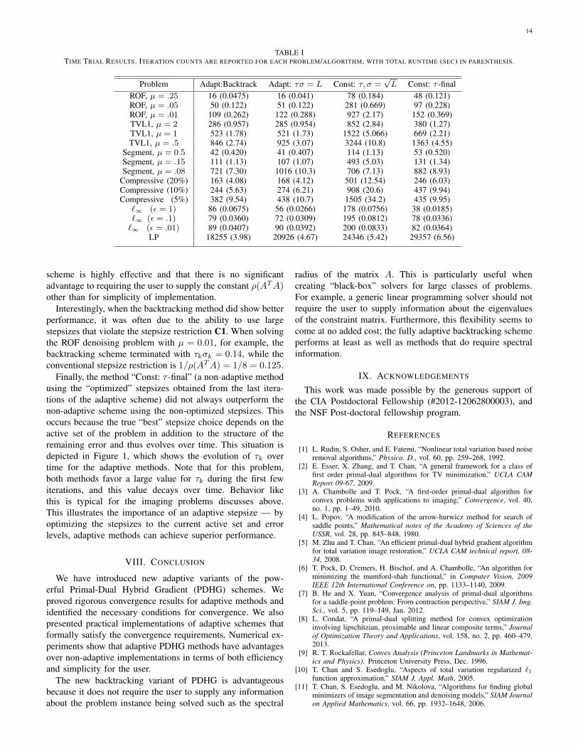
TABLE ITIME TRIAL RESULTS. ITERATION COUNTS ARE REPORTED FOR EACH PROBLEM/ALGORITHM, WITH TOTAL RUNTIME (SEC) IN PARENTHESIS.

Problem Adapt:Backtrack Adapt: τσ = L Const: τ, σ =√L Const: τ -final

ROF, µ = .25 16 (0.0475) 16 (0.041) 78 (0.184) 48 (0.121)ROF, µ = .05 50 (0.122) 51 (0.122) 281 (0.669) 97 (0.228)ROF, µ = .01 109 (0.262) 122 (0.288) 927 (2.17) 152 (0.369)TVL1, µ = 2 286 (0.957) 285 (0.954) 852 (2.84) 380 (1.27)TVL1, µ = 1 523 (1.78) 521 (1.73) 1522 (5.066) 669 (2.21)TVL1, µ = .5 846 (2.74) 925 (3.07) 3244 (10.8) 1363 (4.55)

Segment, µ = 0.5 42 (0.420) 41 (0.407) 114 (1.13) 53 (0.520)Segment, µ = .15 111 (1.13) 107 (1.07) 493 (5.03) 131 (1.34)Segment, µ = .08 721 (7.30) 1016 (10.3) 706 (7.13) 882 (8.93)

Compressive (20%) 163 (4.08) 168 (4.12) 501 (12.54) 246 (6.03)Compressive (10%) 244 (5.63) 274 (6.21) 908 (20.6) 437 (9.94)Compressive (5%) 382 (9.54) 438 (10.7) 1505 (34.2) 435 (9.95)

`∞ (ε = 1) 86 (0.0675) 56 (0.0266) 178 (0.0756) 38 (0.0185)`∞ (ε = .1) 79 (0.0360) 72 (0.0309) 195 (0.0812) 78 (0.0336)`∞ (ε = .01) 89 (0.0407) 90 (0.0392) 200 (0.0833) 82 (0.0364)

LP 18255 (3.98) 20926 (4.67) 24346 (5.42) 29357 (6.56)

scheme is highly effective and that there is no significantadvantage to requiring the user to supply the constant ρ(ATA)other than for simplicity of implementation.

Interestingly, when the backtracking method did show betterperformance, it was often due to the ability to use largestepsizes that violate the stepsize restriction C1. When solvingthe ROF denoising problem with µ = 0.01, for example, thebacktracking scheme terminated with τkσk = 0.14, while theconventional stepsize restriction is 1/ρ(ATA) = 1/8 = 0.125.

Finally, the method “Const: τ -final” (a non-adaptive methodusing the “optimized” stepsizes obtained from the last itera-tions of the adaptive scheme) did not always outperform thenon-adaptive scheme using the non-optimized stepsizes. Thisoccurs because the true “best” stepsize choice depends on theactive set of the problem in addition to the structure of theremaining error and thus evolves over time. This situation isdepicted in Figure 1, which shows the evolution of τk overtime for the adaptive methods. Note that for this problem,both methods favor a large value for τk during the first fewiterations, and this value decays over time. Behavior likethis is typical for the imaging problems discusses above.This illustrates the importance of an adaptive stepsize — byoptimizing the stepsizes to the current active set and errorlevels, adaptive methods can achieve superior performance.

VIII. CONCLUSION

We have introduced new adaptive variants of the pow-erful Primal-Dual Hybrid Gradient (PDHG) schemes. Weproved rigorous convergence results for adaptive methods andidentified the necessary conditions for convergence. We alsopresented practical implementations of adaptive schemes thatformally satisfy the convergence requirements. Numerical ex-periments show that adaptive PDHG methods have advantagesover non-adaptive implementations in terms of both efficiencyand simplicity for the user.

The new backtracking variant of PDHG is advantageousbecause it does not require the user to supply any informationabout the problem instance being solved such as the spectral

radius of the matrix A. This is particularly useful whencreating “black-box” solvers for large classes of problems.For example, a generic linear programming solver should notrequire the user to supply information about the eigenvaluesof the constraint matrix. Furthermore, this flexibility seems tocome at no added cost; the fully adaptive backtracking schemeperforms at least as well as methods that do require spectralinformation.

IX. ACKNOWLEDGEMENTS

This work was made possible by the generous support ofthe CIA Postdoctoral Fellowship (#2012-12062800003), andthe NSF Post-doctoral fellowship program.

REFERENCES

[1] L. Rudin, S. Osher, and E. Fatemi, “Nonlinear total variation based noiseremoval algorithms,” Physica. D., vol. 60, pp. 259–268, 1992.

[2] E. Esser, X. Zhang, and T. Chan, “A general framework for a class offirst order primal-dual algorithms for TV minimization,” UCLA CAMReport 09-67, 2009.

[3] A. Chambolle and T. Pock, “A first-order primal-dual algorithm forconvex problems with applications to imaging,” Convergence, vol. 40,no. 1, pp. 1–49, 2010.

[4] L. Popov, “A modification of the arrow-hurwicz method for search ofsaddle points,” Mathematical notes of the Academy of Sciences of theUSSR, vol. 28, pp. 845–848, 1980.

[5] M. Zhu and T. Chan, “An efficient primal-dual hybrid gradient algorithmfor total variation image restoration,” UCLA CAM technical report, 08-34, 2008.

[6] T. Pock, D. Cremers, H. Bischof, and A. Chambolle, “An algorithm forminimizing the mumford-shah functional,” in Computer Vision, 2009IEEE 12th International Conference on, pp. 1133–1140, 2009.

[7] B. He and X. Yuan, “Convergence analysis of primal-dual algorithmsfor a saddle-point problem: From contraction perspective,” SIAM J. Img.Sci., vol. 5, pp. 119–149, Jan. 2012.

[8] L. Condat, “A primal-dual splitting method for convex optimizationinvolving lipschitzian, proximable and linear composite terms,” Journalof Optimization Theory and Applications, vol. 158, no. 2, pp. 460–479,2013.

[9] R. T. Rockafellar, Convex Analysis (Princeton Landmarks in Mathemat-ics and Physics). Princeton University Press, Dec. 1996.

[10] T. Chan and S. Esedoglu, “Aspects of total variation regularized `1function approximation,” SIAM J. Appl. Math, 2005.

[11] T. Chan, S. Esedoglu, and M. Nikolova, “Algorithms for finding globalminimizers of image segmentation and denoising models,” SIAM Journalon Applied Mathematics, vol. 66, pp. 1932–1648, 2006.

15

[12] T. Goldstein, X. Bresson, and S. Osher, “Geometric applications of theSplit Bregman method: Segmentation and surface reconstruction,” J. Sci.Comput., vol. 45, pp. 272–293, October 2010.

[13] T. Goldstein, X. Bresson, and S. Osher, “Global minimization of markovrandom fields with applications to optical flow,” Inverse Problems inImaging, vol. 6, pp. 623–644, November 2012.

[14] E. Brown, T. Chan, and X. Bresson, “Completely convex formulationof the chan-vese image segmentation model,” International Journal ofComputer Vision, vol. 98(1), pp. 103–121, 2012.

[15] B. Goldluecke and D. Cremers, “Convex Relaxation for MultilabelProblems with Product Label Spaces,” in Computer Vision ECCV 2010(K. Daniilidis, P. Maragos, and N. Paragios, eds.), vol. 6315 of LectureNotes in Computer Science, ch. 17, pp. 225–238, Berlin, Heidelberg:Springer Berlin / Heidelberg, 2010.

[16] E. Bae, J. Yuan, and X. C. Tai, “Global minimization for continuousmultiphase partitioning problems using a dual approach,” Internationaljournal of computer vision, vol. 92, no. 1, pp. 112–129, 2011.

[17] E. J. Candes, J. Romberg, and T.Tao, “Robust uncertainty principles:Exact signal reconstruction from highly incomplete frequency informa-tion,” IEEE Trans. Inform. Theory, vol. 52, pp. 489 – 509, 2006.

[18] E. J. Candes and J. Romberg, “Signal recovery from random projec-tions,” Proc. of SPIE Computational Imaging III, vol. 5674, pp. 76 –86, 2005.

[19] M. Duarte, M. Davenport, D. Takhar, J. Laska, T. Sun, K. Kelly, andR. Baraniuk, “Single-pixel imaging via compressive sampling: Buildingsimpler, smaller, and less-expensive digital cameras,” Signal ProcessingMagazine, IEEE, vol. 25, no. 2, pp. 83–91, 2008.

[20] S. H. Han and J. H. Lee, “An overview of peak-to-average power ratioreduction techniques for multicarrier transmission,” Wireless Communi-cations, IEEE, vol. 12, no. 2, pp. 56–65, 2005.

[21] C. Studer, W. Yin, and R. G. Baraniuk, “Signal representations withminimum l∞-norm,” in Proc. 50th Annual Allerton Conference onCommunication, Control, and Computing, 2012.

[22] J. A. Cadzow, “Algorithm for the minimum-effort problem,” AutomaticControl, IEEE Transactions on, vol. 16, no. 1, pp. 60–63, 1971.

[23] H. Jegou, T. Furon, and J. J. Fuchs, “Anti-sparse coding for approximatenearest neighbor search,” in ICASSP - 37th International Conference onAcoustics, Speech, and Signal Processing, (Kyoto, Japan), Jan. 2012.Quaero.

[24] J. Duchi, S. S. Shwartz, Y. Singer, and T. Chandra, “Efficient projectionsonto the `1-ball for learning in high dimensions,” in Proc. of the 25thinternational conference on Machine learning, ICML ’08, (New York,NY, USA), pp. 272–279, ACM, 2008.

[25] A. Schrijver, Combinatorial Optimization: Polyhedra and Efficiency.Springer, 2003.

[26] T. Pock and A. Chambolle, “Diagonal preconditioning for first orderprimal-dual algorithms in convex optimization,” in Computer Vision(ICCV), 2011 IEEE International Conference on, pp. 1762–1769, 2011.

[27] B. He, H. Yang, and S. Wang, “Alternating direction method withself-adaptive penalty parameters for monotone variational inequalities,”Journal of Optimization Theory and Applications, vol. 106, no. 2,pp. 337–356, 2000.

[28] S. Boyd, N. Parikh, E. Chu, B. Peleato, and J. Eckstein, “DistributedOptimization and Statistical Learning via the Alternating DirectionMethod of Multipliers,” Foundations and Trends in Machine Learning,2010.

[29] H. Bauschke and P. Combettes, Convex Analysis and Monotone OperatorTheory in Hilbert Spaces. Springer, 2011.