Document Number: SET 2014-0039 412TW-PA-14271

Adaptive Modulation Schemes for OFDM and SOQPSK Using Error Vector Magnitude (EVM)

and Godard Dispersion

June 2014

Final Report

Tom Young SET Executing Agent 412 TENG/ENI (661) 277-1071 Email: tommy.young.1@us.af.mil

Approved for public release; distribution is unlimited.

Controlling Office: 412 TENG/ENI, Edwards AFB, CA 93524

Test Resource Management Center (TRMC) Test & Evaluation/ Science & Technology (T&E/S&T)

Spectrum Efficient Technology (SET)

REPORT DOCUMENTATION PAGE Form Approved

OMB No. 0704-0188 Public reporting burden for this collection of information is estimated to average 1 hour per response, including the time for reviewing instructions, searching existing data sources, gathering and maintaining the data needed, and completing and reviewing this collection of information. Send comments regarding this burden estimate or any other aspect of this collection of information, including suggestions for reducing this burden to Department of Defense, Washington Headquarters Services, Directorate for Information Operations and Reports (0704-0188), 1215 Jefferson Davis Highway, Suite 1204, Arlington, VA 22202- 4302. Respondents should be aware that notwithstanding any other provision of law, no person shall be subject to any penalty for failing to comply with a collection of information if it does not display a currently valid OMB control number. PLEASE DO NOT RETURN YOUR FORM TO THE ABOVE ADDRESS. 1. REPORT DATE (DD-MM-YYYY)03-06-2014

2. REPORT TYPETechnical Paper

3. DATES COVERED (From - To)3/13 -- 3/16

4. TITLE AND SUBTITLEAdaptive Modulation Schemes for OFDM and SOQPSK Using Error Vector Magnitude (EVM) and Godard Dispersion

5a. CONTRACT NUMBER: W900KK-13-C- 0024 5b. GRANT NUMBER: N/A

5c. PROGRAM ELEMENT NUMBER

6. AUTHOR(S)

Jieying Han, Brett T. Walkenhorst, Enkuang D. Wang

5d. PROJECT NUMBER

5e. TASK NUMBER

5f. WORK UNIT NUMBER

7. PERFORMING ORGANIZATION NAME(S) AND ADDRESS(ES)

Attn: Brett Walkenhorst Georgia Tech Applied Research Corporation, 505 10TH ST Atlanta GA 30332-0001

8. PERFORMING ORGANIZATION REPORTNUMBER

412TW-PA-14271

9. SPONSORING / MONITORING AGENCY NAME(S) AND ADDRESS(ES)Test Resource Management Center Test and Evaluation/ Science and Technology 4800 Mark Center Drive, Suite 07J22 Alexandria, VA 22350

10. SPONSOR/MONITOR’S ACRONYM(S)N/A

11. SPONSOR/MONITOR’S REPORTNUMBER(S) SET 2014-0039

12. DISTRIBUTION / AVAILABILITY STATEMENT Approved for public release A: distribution is unlimited.

13. SUPPLEMENTARY NOTESCA: Air Force Flight Test Center Edwards AFB CA CC: 012100

14. ABSTRACTIn this paper, we develop a new approach which enables adaptation across two modulation schemes in the iNET standard: orthogonal frequency-division multiplexing (OFDM) and shaped-offset quadrature phased-shift keying (SOQPSK). We present the error vector magnitude (EVM) for OFDM and second-order Godard dispersion (D(2)) for SOQPSK as our link metrics that measure the degradation due to thermal noise and channel effects and then derive the mathematical relationship between these two metrics. This relationship enables us to utilize a set of empirically-derived rules that incorporate both modulation schemes.

15. SUBJECT TERMSSpectrum, Aeronautical telemetry, algorithm, bandwidth, Orthogonal Frequency Division Multiplexing (OFDM), Shaped Offset Quadrature Phase Shift Keying (SOQPSK), Using Error Vector Magnitude (EVM), Godard Dispersion (D(2))

16. SECURITY CLASSIFICATION OF:Unclassified

17. LIMITATIONOF ABSTRACT

None

18. NUMBEROF PAGES

15

19a. NAME OF RESPONSIBLE PERSON 412 TENG/EN (Tech Pubs)

a. REPORT Unclassified

b. ABSTRACTUnclassified

c. THIS PAGEUnclassified

19b. TELEPHONE NUMBER (include area code)

661-277-8615 Standard Form 298 (Rev. 8-98) Prescribed by ANSI Std. Z39.18

DISTRIBUTION LIST

Onsite Distribution Number of Copies

E-Mail Digital Paper

Attn. Tom Young, SET Executing Agent 412 TENG/ENI 61 N. Wolfe Ave. Bldg 1632 Edwards, AFB, CA 93524

0 2 2

Attn: Brett Walkenhorst Georgia Tech Applied Research Corporation 505 10TH ST Atlanta GA 30332-0001 Brett.Walkenhorst@gtri.gatech.edu

1 0 0

Attn: Jieying Han Georgia Tech Applied Research Corporation 505 10TH ST Atlanta GA 30332-0001

0 1 0

Attn: Enkuang D. Wang Georgia Tech Applied Research Corporation 505 10TH ST Atlanta GA 30332-0001

0 1 0

Edwards AFB Technical Research Libaray Attn: Darrell Shiplett 307 East Popson Ave, Bldg 1400 Edwards AFB CA 93524

0 2 2

Offsite Distribution

Defense Technical Information Center

1

0

0 DTIC/O 8725 John J Kingman Road, Suite 0944 Ft Belvoir, VA 22060-6218

U.S. ARMY PEO STRI Acquisition Center Email to: kaitlin.lockett@us.army.mil Attn: Kaitlin F. Lockett 12350 Research Parkway Orlando, FL 32826

1 0 0

1

ADAPTIVE MODULATION SCHEMES FOR OFDM AND SOQPSK USING ERROR VECTOR MAGNITUDE (EVM) AND

GODARD DISPERSION

Jieying Han, Brett T. Walkenhorst, Enkuang D. Wang Georgia Tech Research Institute

Atlanta, Georgia, USA

ABSTRACT In this paper, we develop a new approach which enables adaptation across two modulation schemes in the iNET standard: orthogonal frequency-division multiplexing (OFDM) and shaped-offset quadrature phased-shift keying (SOQPSK). We present the error vector magnitude (EVM) for OFDM and second-order Godard dispersion (D(2)) for SOQPSK as our link metrics that mea- sure the degradation due to thermal noise and channel effects and then derive the mathematical relationship between these two metrics. This relationship enables us to utilize a set of empirically- derived rules that incorporate both modulation schemes.

I. INTRODUCTION In current telemetry systems, a constant phase modulation (CPM) scheme such as CPM-FM or SOQPSK is typically used to transmit data from an airborne test article (TA) to a receiving ground station (GS). The chosen scheme will have a fixed data rate and coding rate and be unable to adapt its transmission to changing channel conditions. In an attempt to improve the spectral efficiency of such telemetry systems, the Georgia Tech Research Institute (GTRI) is developing an adaptive modulation and coding capability called link-dependent adaptive radio (LDAR). The main purpose of the algorithm is to maximize the throughput of the telemetry link while maintaining a minimum level of reliability, measured as bit error rate (BER). In order to accomplish this objective, the channel must be estimated and link quality assessed to determine what mode of operation would meet the objective. Multiple parameters may be changed in attempting to maximize throughput while maintaining link quality, such as modulation types, forward error correction schemes and rate, signal bandwidth, and number of sub-carriers.

The idea of adapting modulation and other parameters to meet the demands of the current channel

2

is not new; there have been numerous papers published on the idea such as [1,2], and others. How- ever, these implementations are somewhat limited in scope compared to what we proposed in the LDAR project, and very few studies address the adaptation of so many parameters simultaneously.

This paper focuses on enabling adaptation across two modulation schemes found in the iNET standard: OFDM and SOQPSK. Seeking to find metrics that measure degradation due to thermal noise and channel effects, we chose error vector magnitude (EVM) as our metric for OFDM. This metric measures the difference between the received symbols and their expected positions in the I/Q plane. Because of the partial response filter of SOQPSK and its associated method of demod- ulation using the Viterbi decoder [3] or similar decoding method such as the BCJR’s sequential decoding scheme [4], EVM has no meaning for SOQPSK since there is no soft decision in the demodulation of the signal. We therefore chose a metric called second-order Godard dispersion, defined as D(2) = E[(|y(n)|)2 − R2)2] where y(n) is the received signal and R2 is the amplitude of the constant modulus signal, to measure the quality of a received SOQPSK signal. This metric measures the width modulus error of a constant modulus signal and therefore captures the effects of both thermal noise and channel effects. In order to dynamically adapt the modulation type be- tween these two schemes, we derive in this paper the mathematical relationship between EVM and Godard dispersion, which enables us to utilize a set of empirically-derived adaptation rules that incorporate both modulation schemes.

The paper is organized as follows. Section II introduces the SOQPSK and OFDM modulation schemes that are used in aeronautical telemetry applications. In Section III, we present the link metrics of EVM and Godard dispersion (D(2)). Section IV develops the mathematical relationship between EVM and D(2), followed by numerical results in Section V. Finally, we conclude the paper in Section VI and discuss our future work.

II. MODULATION SCHEMES Description of SOQPSK The SOQPSK modulation scheme [6–8] is defined as a continuous phase modulation (CPM) with baseband modulated signal expressed as

Eb

x(t) = exp[j(φ(t, α) + φ0)] (1) b

where Eb is energy per bit, Tb is the bit duration, φ0 is an arbitrary phase that will be set to 0 for this work, and the information carrying phase is given by

r t φ(t, α) = 2πh

∞ \ αng(τ − nTb)dτ (2)

−∞ n=−∞

where g(t) is the frequency pulse, h = 1/2 is the modulation index, and αn ∈ {−1, 0, 1} are the ternary input symbols, which are related to the binary data bits bn ∈ {0, 1} by

αn = (−1)n+1(2bn −1 − 1)(bn — bn−2 ). (3)

T

3

2T 2T

2Tb

2Tb

l=0

l=0

Different versions of SOQPSK differ by their respective frequency pulse. In this paper, we use the telemetry version SOQPSK-TG, which is partial-response with pulse duration of L = 8 and a frequency pulse given by the product of a raised-cosine frequency-domain window and time- domain window given by the following expression

g(t) = C

cos( πβ1β2t ) b

sin( πβ2t ) b

w(t)

(4)

1 − 4( β1β2t )2 πβ2t 2Tb 2Tb Time-domain

where

Frequency-d o main window window

1 0 ≤ | t | < T1

w(t) =

1 + 1 cos( π ( t − T1)) T1 ≤ | t | ≤ T1 + T2 (5) 2 2 T2 2Tb 2Tb 0 T1 + T2 < | t |

According to the iNET standard [5], the parameters are β1 = 0.7, β2 = 1.25, T1 = 1.5, and T2 = 0.5. The constant C is chosen to make g(t) = 1/2 for t ≥ 2(T1 + T2)Tb.

The discrete-time SOQPSK system model is presented in Fig.1, where xn is a discrete-time SO- QPSK waveform, hl is the multipath channel impulse response, L is the channel length and wn is an additive white Gaussian noise. The output of the channel yn can be written as

L−1

yn = h ∗ xn + wn = \

xn l=0

Multipath Channel

−lhl

+ wn

. (6)

Input

Bits

Encoder SOQPSK xn

Mod {hl}L−1

yn SOQPSK ut Demod

Figure 1: SOQPSK system model

Description of OFDM The OFDM [9] implementation is illustrated in Fig.2.

S(i)

S(i)

Y (i)

x(i)

y(i)

P/S, Add

Prefix

{hl}L−1 h

w Output

Bits

Figure 2: OFDM system model

At each OFDM block index i, a set of N QAM symbols S(i) = {S(i)}N−1 is transmitted over N k k=0

P/S Symbol Demap, Decoder

Multipath Channel

Decoder

Outp Bits

S/P

IFFT

Equalizer

FFT

Remove Prefix,

S/P

4

m

l=0

y

.

(i)

1 . .

.

sub-carriers and these frequency components are converted into time samples by performing an inverse DFT (IFFT). After parallel to serial conversion, a cyclic redundancy of length v is added as a prefix in such a way that x(i)

−

(i) N−m , m = 1, 2, ...v and the signal is then serially transmitted

over a noisy multipath channel with channel impulse response (CIR) {hl}L−1. If the Cyclic Prefix length is at least as long as the CIR length (v ≥ L) [10], the received signal y(i) can be expressed in terms of x(i) and noise vector w as

x(i) −.

v (i) 0

hv · · · h0 0 · · · · · · 0

.. w0

y(i) . . . . . . ..

(i) w 1 0 . . . .

x0

1 . .. . . . . . . ..

x

+

.. .. = . . . . . . . . (i) .

..

. (7) . .. . . . . . . . . . 0 ..

.. .. wN 1 (i)

N−1 0 · · · · · · 0 hv · · · h0

−

(i) N−1

The received symbols y(i) , · · · , y(i) are discarded since they may be affected by ISI from the

−1 −v prior data block, and they are not needed to recover the input signal. The first v symbols of x(i) correspond to the cyclic prefix: x(i)

−

(i) N−1 , · · · , x−v

(i) N−v . We therefore write (7) as

y(i) = Hcircx(i) + w (8) where Hcirc is an N × N circulant matrix with an eigenvalue decomposition of

Hcirc = QH ΛQ (9) where Q ∈ CN×N is the normalized Discrete Fourier Transform (DFT) matrix (note that Q is unitary i.e. QQH = IN ), and the diagonal matrix Λ contains the eigenvalues of the circulant matrix. These values can be written as

Λ = diag(Q

I h

0N−L

l \ � H. (10)

The matrix H is defined to be a diagonal matrix containing the channel frequency response coef- ficients along its main diagonal.

Taking the FFT of (8), we find

Y (i) = Qy(i)

= Q(Hcircx(i) + w) = Q(HcircQH S(i) + w) = Q(QH HQQH S(i) + w) = HS(i) + w

(11)

where w = Qw. After equalization [11], the estimated symbol S(i)

is given as

S(i)

= H−1Y (i) = H−1(HS(i) + w ) = S(i) + H−1w

(12)

= x

y x

1 = x = x

5

1

III. LINK METRICS Based on the system models introduced from the previous section, we want to find a common met- ric that will allow us to adapt our transmissions over both of these modulation schemes. However, there is no such a common metric that exists for both modulation schemes, we therefore chose EVM as our metric for OFDM and Godard dispersion for SOQPSK.

In order to adapt over both OFDM and SOQPSK with two distinct metrics, we need to find the relationship between EVM and Godard dispersion. The two metrics are detailed in the following.

Error Vector Magnitude (EVM) EVM measures the deviation of the received symbols from their original transmitted positions in the I/Q plane. Fig.3 shows the normalized constellation di- agram for QPSK with one received symbol. It has been shown that EVM normalization enables direct comparison for a given average power level per symbol between modulation types (i.e., BPSK, QPSK,16QAM, 64QAM, etc) [12].

Q Received Symbol

1 Error Vector Original Symbol

I

Figure 3: Normalized constellation diagram for QPSK EVM is defined as the root-mean-square (RMS) value of the difference between a collection of re- ceived symbols and the original transmitted symbols. These differences are averaged over a given, typically large, number of symbols and are often shown as a percentage of the average power per symbol of the constellation, or mathematically:

1

Ns 2 2 \

Sr,i − So,i

Ns

EVMRMS =

i=1

1 Ns

Ns \

i=1

2

o,i

, (13)

where Sr,i is the received symbol, So,i is the original transmitted symbol, and Ns is the number of symbols over which EVM is averaged. In this paper, we use

EVM = (EVMRMS)2. (14)

Godard Dispersion Function (Cost Function) Godard dispersion function [13] was first pro- posed by Godard [14], and is defined as

D(p) = E[(|yn|p − Rp)2] (15)

S

6

2

2

2

l

w

\

\

S

N

l

N

N

N

E[|xn|2p] (16) Rp � E[|xn| ]

where xn is the input symbol, yn is the received symbol, Rp is a constant depending only on the input data constellation, p is an integer. For p = 2, the special Godard algorithm was developed as the Constant Modulus algorithm (CMA) independently by Treichler and co-workers [15], and the CMA is widely used for blind equalization. In this paper, we use p = 2.

IV. RELATIONSHIP BETWEEN EVM AND GODARD DISPERSION Based on the description of EVM and Godard dispersion from the previous section, we now seek to relate the two metrics.

EVM for OFDM Assume the transmit symbol S(i) is one OFDM block (with N sub-carriers) normalized to unit energy and S

(i) denotes the estimated symbol defined in (12), the EVM is

defined as follows:

(i)

EVM = E[lS (i)

— l E[lS(i)l ] 1 (i)

= N E[lS 1

− S(i)l2] 2

= E[lS(i) + H−1w − S(i)l ] =

1 E[ H−1w 2]

N

= 1

E[(H−1w)H (H−1w)] N

= 1

E[T r{(H−1w)(H−1w)H }]

= 1

T r{E[H−1wwH (H−1)H ]}

= 1

T r{H−1σ2 I(H−1)H} N

= σ2 1 |H−1|2 (17) w N jj

jj=1

where Hjj is the jth diagonal element of H (defined in (10)) . As w = Qw, we have

E[wwH ] = E[(Qw)(Qw)H ] = E[QwwH QH ] = Qσ2 IQH = σ2 I (18)

Thus w ∼ CN (0, σ2 I) and σ2

w w = σ2 . Therefore,

w w w

EVM = σ2 1

N |H−1|2 (19)

w N jj jj=1

ˆ

ˆ

]

7

w

x

l=0

2

w

1 },N jj |

Godard Dispersion for SOQPSK Let xn denote the transmitted complex signal, yn denote the received signal, h denote the channel impulse response of length L, and wn denote the noise with distribution w ∼ CN (0, σ2 I). The received signal is then given by yn = h ∗ xn + wn. Assume we normalize the transmitted signal to unit energy: E[ |xn|2] = σ2 = 1, and the channel has unit energy:

},L−1 |hl|2 = 1. The second-order Godard dispersion (D(2)) for SOQPSK is defined as:

D(2) = EI(|yn|2 − 1

\ l (20)

We model xn as a complex variable with zero mean and variance σ2. Given E[(xn)2] = E[(x∗ )2] = x n

E[xn] = 0, we find the following (see Appendix for the complete derivation):

L−1 L−1 L−1 D(2) = 2

\ \ |hl|2|hp|2 −

\ |hl|4 + 2σ4 + 2σ2 − 1 (21)

l=0 p=0

w w l=0

Mapping Between EVM and Godard Dispersion From the previous sections, we have ex- pressed EVM and second-order Godard Dispersion in terms of the noise variance and channel impulse response. We now relate these metrics to one another by solving for σ2 in (19) and sub- stituting into (21) to obtain

L−1 L−1

L−1 EVM 2 EVM D(2) = 2

\ \ |hl|2|hp|2 −

\ |hl|4 + 2

I(

\ +

1 2 1 N

l 1 (22) −1

l=0 p=0 l=0 N jj=1 |H− }, N jj=1

|Hjj |2

where N is the number of sub-carriers, hi is channel impulse response and Hjj is the frequency- domain channel response of the jth subcarrier.

V. SIMULATION RESULTS We now perform simulations to compare our theoretical mapping to metrics computed from time- domain simulated data using an AWGN channel. The theoretical data is calculated using (19) and (21), the simulated data is calculated using (13) and (15) with simulated SOQPSK and OFDM waveforms. The simulation results were obtained using 2/3 low density parity check (LDPC) code rate. The EVM values were calculated using OFDM/QPSK with 64 sub-carriers. Both EVM and D(2) were simulated using 100 iNET bursts, each burst consists of 49152 coded bits (8 LDPC codeblocks).

Table 1 presents our results using SNR = −5 dB, 0 dB and 15 dB, the simulated data of EVM and D(2) are both very close to the theoretical data, which verifies our mathematical expressions in (19) and (21). The “mapped D(2) from EVM” is essentially identical to the theoretical D(2), which verifies our mathematical mapping in (22).

More simulation results are shown in Fig.4 with SNR ranges from −5 dB to 20 dB. The top figure is for EVM while the bottom is for Godard dispersion (D(2)). It can be seen from the figure that the simulated EVM and D(2) are both very close to the theoretical data, the average percentage error

−

8

between “mapped D(2) from EVM” and “theoretical D(2)” is only about 0.0682%.

8

Table 1: Simulation results comparing to theoretical results

SNR(dB) EVM Godard Dispersion (D(2)) Theoretical Simulated Theoretical Simulated Mapped from EVM

-5 3.1623 3.1642 26.3246 26.3318 26.3525 0 1.0000 0.9993 4.0000 3.9968 3.9960 15 0.0316 0.0316 0.0652 0.0652 0.0652

Figure 4: Simulation results comparing to theoretical results

VI. CONCLUSION We presented a theoretical mapping between two metrics to enable the adaptation across two mod- ulation schemes in the iNET standard: OFDM and SOQPSK. We derived the mathematical map- ping from EVM to second-order Godard dispersion, which enables us to utilize a set of empirical adaptation rules that incorporate both modulation schemes [16]. Moreover, we verified our map- ping using an AWGN channel with experimental results very close to theoretical results. Future work will integrate this mapping to our adaptation rules in [16] and test using representative chan- nel models we have developed; then we will implement these rules in hardware and test in real wireless channels.

ACKNOWLEDGMENTS

The authors would like to thank the Test Resource Management Center (TRMC) Test and Evalu- ation/Science and Technology (T&E/S&T) Program for their support. This work was funded by the T&E/S&T Program through the U.S. Army Program Executive Office for Simulation, Training and Instrumentation (PEO STRI), contract number W900KK-13-C-024 for link-dependent adap- tive radio (LDAR). The public release approval number for this paper is 412TW-PA-14271.

9

References [1] A.J. Goldsmith and S.G. Chua, “Adaptive coded modulation for fading channels,” IEEE Trans-

actions on Communications, Vol. 46, No. 5, pp. 595-602, 1998.

[2] A. Svensson, “An introduction to adaptive QAM modulation schemes for known and predicted channels,” Proceedings of the IEEE, Vol. 95, No. 12, pp. 2322-2336, 2007.

[3] J. Huber and W. Liu, “An alternative approach to reduced-complexity CPM-receivers,” Se- lected Areas in Communications, IEEE Journal on, vol. 7, no. 9, pp. 1437-1449, Dec. 1989.

[4] L.Bahl, J.Cocke, F.Jelinek, and J.Raviv, “Optimal decoding of linear codes for minimizing symbol error rate,” IEEE Transactions on Information Theory, vol. IT-20(2), pp. 284-287, Mar. 1974.

[5] integrated Network Enhanced Telemetry (iNET) Radio Access Network Standards Working Group, “Radio access network (RAN) standard, version 0.7.9,” Mar. 2013.

[6] T. Nelson, E. Perrins, and M. Rice, “Near optimal common detection techniques for shaped offset QPSK and Feher’s QPSK,” IEEE Transactions on Communications, vol. 56, no. 5, pp. 724-735, May 2008.

[7] E. Perrins and M. Rice, “Reduced-complexity approach to iterative detection of SOQPSK,” IEEE Trans. Commun., vol. 55, no. 7, pp. 1354-1362, July 2007.

[8] J. Proakis and M. Salehi, Digital Communications, McGraw-Hill, Inc. New NY, 2008.

[9] Andrea Goldsmith, Wireless Communications, Cambridge University Press, 2005.

[10] M. Danish Nisar, “OFDM Systems - Why Cyclic Prefix” A tutorial on OFDM systems, [on- line] (available: http://www.ict.kth.se/courses/IL2205/OFDM Tutorial.pdf)

[11] P. Schniter, “Low-complexity equalization of OFDM in doubly selective channels,” IEEE Trans. Signal Processing, vol. 52, pp. 1002-1011, Apr. 2004.

[12] M. D. McKinley, K. A. Remley, M. Myslinski, J. S. Kenney, D. Schreurs and B. Nauwelaers, “EVM calculation for broadband modulated signals” 64th ARFTG Conf. Dig., pp. 45-52, 2004.

[13] H. V. Poor and L. Tong, Signal Processing for Wireless Communication Systems, Kluwer Academic, 2002.

[14] D. N. Godard, “Self-recovering equalization and carrier tracking in two-dimensional data communications systems,” IEEE Trans. Commun., vol. 28, no. 11, pp. 1867-1875, Nov. 1980.

[15] J. R. Treichler and B. G. Agee, “A new approach to multipath correction of constant modulus signals,” IEEE Trans. Acoust., Speech, Signal Process., vol. 31, no. 2, pp. 459-472, Apr. 1983.

[16] E. D. Wang, B. T. Walkenhorst and J. Han, “A simulation testbed for airborne telemetry applications,” in Proceedings of the International Telemetering Conference, San Diego, CA, Oct. 2014

10

(

n l l w

n−l l

2

n

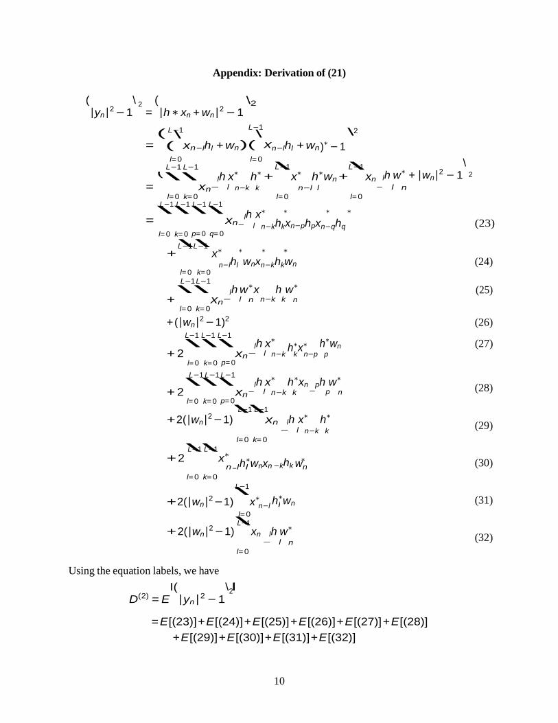
Appendix: Derivation of (21)

(|yn|2 − 1

\ =

(|h ∗ xn + wn|2 − 1

L−1

\2

L−1 2

= ((\

xn

l=0 −lhl + wn )(

\ x

l=0 n−lhl + wn

\ )∗ − 1

L−1 L−1

= \ \

xn lh x∗

L−1 h∗ + \

x∗ L−1

h∗wn + \

xn lh w∗ + |wn|2 − 1\

l=0 k=0 — l n−k k

l=0 n−l l

l=0 — l n

L−1 L−1 L−1 L−1

= \ \ \ \

xn

lh x∗ ∗ ∗ ∗

l=0 k=0 p=0 q=0

L−1 L−1

— l n−khkxn−phpxn−qhq (23)

+ \ \

x∗ ∗ ∗ ∗

l=0 k=0 L−1 L−1

n−lhl wnxn−khkwn (24)

+ \ \

xn lh w∗x h w∗ (25)

l=0 k=0 — l n n−k k n

+ (|wn|2 − 1)2 (26) L−1 L−1 L−1

+ 2 \ \ \

xn lh x∗ h∗x∗ h∗wn (27)

l=0 k=0 p=0

L−1 L−1 L−1

— l n−k k n−p p

+ 2 \ \ \

xn lh x∗ h∗xn ph w∗

l=0 k=0 p=0 — l n−k k — p n

L−1 L−1 + 2(|wn|2 − 1)

\ \ xn lh x∗ h∗

L−1 L−1 l=0 k=0

— l n−k k

+ 2 \ \

x∗ − h

∗wnxn −khk ∗

l=0 k=0 L−1

+ 2(|wn|2 − 1) \

x∗ h∗wn

l=0 L−1

+ 2(|wn|2 − 1) \

xn lh w∗

Using the equation labels, we have

l=0 — l n

D(2) = EI(|yn|2 − 1

\ l

= E[(23)] + E[(24)] + E[(25)] + E[(26)] + E[(27)] + E[(28)] + E[(29)] + E[(30)] + E[(31)] + E[(32)]

2

2

(28)

(29)

(30)

(31)

(32)

11

|

l

n

w w

h

n

E

Approaching these in turn, we have L−1 L−1

E[(23)] = \ \

l=0 p=0

(l=k,p=q,l/=p)

|hl|2|hp|2EI|xn 2

l I −l| E |x 2

l n−p|

L−1 L−1

+ \ \ l=0 k=0

(l=q,k=p,l/=k)

L−1

|hl|2|hk|2EI|xn 2

l I −l| E |x 2

l n−k|

+ \ l=0

(l=k=p=q)

|hl|4EI|xn 4

l l + 0

(others)

L−1 L−1 L−1

= 2 \ \

|hl|2|hp|2 − \

|hl|4

l=0 p=0 l L−1 I

l=0 l I l I l

EI(24)

l

= \

E l=0 L−1

∗ n−l

I

)2 E l

(h∗)2 E I l I

(wn)2 = 0

l E

I(25)

l = \

E l=0 I

(xn l)2 E (hl)2 E l

(w∗ )2 = 0

EI(26) = E |wn|4 + 1 − 2|wn|2

= 2σ4 + 1 − 2σ2

I l (27)

L−1 L−1 L−1

= 2 \ \ \

E Ixn

lx∗

w

x∗ lE

w Ihlh∗h∗

lE

Iwn

l = 0

l=0 k=0 p=0

l L−1 l−1 L−1 I

— n−k n−p

l I

k p

l I l E

I(28) = 2

\ \ \ E xn

lx∗ xn p E h h∗hp E w∗ = 0

l=0 k=0 p=0 l L−1

— n−k − l k n

I l E

I(29) = 2(σ2 − 1)

\ |hl|2E

l=0 L−1 L−1

|xn 2

−l| = 2(σ2 − 1)

L−1 I l (30) = 2 \ \

E Ix∗

xn k lE

I h∗hk lE

I wnw∗ l = 2 \

σ2σ2 |hl|2 = 2σ2

l=0 k=0

l I n−l — l

l L−1 I n

l I l

x w w l=0

EI(31)

l

= 2E wn(|wn|2 − 1)

I l

\ E

l=0 L−1

∗ ∗ n−l l

I l I l

EI(32) = 2E w∗ (|wn|2 − 1) \

E

l=0

xn−l E hl = 0

Finally, we have D(2) as follows: L−1 L−1

L−1 D(2) = 2

\ \ |hl|2|hp|2 −

\ |hl|4 + 2σ4 + 2σ2 − 1

l=0 p=0

w w l=0

(x

E

E

x

−

−

= 0