adaptive methods for nonlinear structural dynamics and crashworthiness analysis · pdf...
TRANSCRIPT

_-_ -3_ _
/,_-7_3 z---÷
f
N94-19466
Adaptive Methods for Nonlinear StructuralDynamics and Crashworthiness Analysis
Ted BelytschkoNorthwestern University
7
https://ntrs.nasa.gov/search.jsp?R=19940014993 2018-05-21T23:42:09+00:00Z


ADAPTIVE METHODS FOR NONLINEAR STRUCTURALDYNAMICS AND CRASHWORTHINESS ANALYSIS
Ted BelytschkoNorthwestern University
Evanston, Illinois
ABSTRACT
The objective of this talk is to describe three research thrusts in crashw0rthiness analysis:
!) aclaptivity2) mixed time integration, or subcycling, in which different timesteps are used for different parts of
the mesh in explicit methods3) methods for contact-impact which are highly vectorizable.
The techniques are being developed to improve the accuracy of calculations, ease-of-use ofcrashworthiness programs and the speed of calculations. The latter is still of importance becausecrashworthiness calculations are often made with models of 20,000 to 50,000 elements using explicit timeintegration and require on the order of 20 to 100 hours on current supercomputers.
The methodologies will be briefly reviewed and then some example calculations employing thesemethods will be described. The methods are also of va_ tobther nonlinear transient computations.
¢
P.'_EOIEDiNG PAGE -gLANK NOT FILleD _ _ :,_:..... £ _ 9
OUTLINE
Adaptive mesh procedures in nonlinearanalysis: why, how, and what is thestatus
• Subcycling (mixed time integration)
New highly vectorizable methods forcontact impact which are well suited toadaptive methods
Figure 1
PREDICTION
The 1990's will be the decade of adaptivity.
adaptive mesh refinement
adaptive targeting
-- .k .
adaptive organization objectives
Figure 2
10

PREDICTION
There are three types of adaptivity, which are known by the letters r, h, and p. These letters aremnemonic letters and refer to how the refinement is achieved. In r methods the nodes are relocated. In h
methods, refinement is achieved by reducing the element size h. In p methods, refinement is achieved byincreasing the order p of the element interpolance.
TYPE OF MESH ADAPTIVITY
r-- method
relocate nodes
h- method
_"---adapt element size h
p- method
_'--adapt order p of element interpolants
Figure 3
ll

ADAPTIVITY IN NONLINEAR FEM
Adaptive methods are particularly useful in nonlinear problems such as crashworthiness becausenonlinear response is often characterized by localization. In the areas of localized response moreref'mement is needed. When standard method is used, the user of the program must refine the mesh wherehe anticipates this localized deformation. Therefore, different meshes must be developed for differentloadings. For example, in car crash, different meshes must be developed for frontal and rear impact, sideimpact, and overturning. This can be quite expensive from the viewpoint of manpower.
Why are adaptive methods particularly important in nonlinearproblems?
Modes of failure of structures
i. buckling, particularly with formation of hingelines
ii. localization
iii. fracture
All of these involve local phenomena whose location cannot bedetermined at the outset of a simulation.
Figure 4
12

COMMENTS ON ADAPTIVITY FOR SHELL ANDCRASHWORTHINESS PROBLEMS
In comparing the different types of adaptivity for nonlinear structural dynamics problems such ascrashworthiness, the following advantages, which are marked by a plus sign (+), and disadvantageswhich are marked by a minus sign (-), can be attributed to the various types of methods. From this studywe concluded that the h-method was the most suitable method for adaptivity in crashworthiness.
m method
- large elements cannot represent shape of shell
+ most accuracy with given NDOF compared to h
- history diffusion
- elements become distorted - decreases accuracy
+ easiest data structure
p m method
- awkward in nonlinear dynamics; no good lumped mass
+ easy data structure
method
+
+
m
relatively effective
no distortion of elements
moderately complex data structure
Figure 5
13

TYPES OF ERROR INDICATORS
Error indicators are an important ingredient in adaptive methods since they are to a guide the refinementof the mesh. Error indicators are classified by Oden in the following classes: residual, interpolation, andpost-processing. In the work we are doing, we are using projection error criterions, a post-processingtype, because they are very easy to implement and are quite effective for low-order elements.
1. Residual: Compute residual in governing equations and use itsnorm or use it to drive an element or local enriched solution.
a) Explicit: Evaluate a norm of the residual.
b) Implicit: Use residual to drive a local or element errorequation•
• Interpolation Methods: Estimate magnitude of derivatives ofhigher-order than contained in finite element space.
• Projection (postprocessing) Methods: Obtain a smoothed solutionand compare to finite element solution; sometimes called L2projection methods.
Figure 6
14

ADAPTIVE SCHEMES FOR TRANSIENT ANDNONLINEAR PROBLEMS
based on constant resource approach
1. Advance the solution n time steps
2. Compute element error indicators 0e
3. Sort 0e
. Fission elements with 0e > tolfusion
Fuse elements with 0e < tolfusion
5. Repeat the last n time steps with new mesh (optional)
6. go to 1
Note: If n is too small or tolfission too close to tolfusion, we
encounter "churning" which degrades accuracy. Our recentexperience shows 5 is quite important.
Figure 7
15

REMARKS ON H-ADAPTIVITY
Constraints (or slave nodes in explicit methods) must be introducedat nodes where a large element has two or more neighbors on oneside to enforce compatibility; easy in vector methods, awkward inmatrix methods.
Usually a group of contiguous elements should be fissionedsimultaneously because fissioning a single element does not providemuch enrichment; only one new free node.
In wave propagation problems, change in element size can causespurious reflections.
Usually mesh gradation is limited to 1-irregular meshes: largeelement cannot have more than 2 small neighbors on any side; seeDevloo, Oden and Strouboulis (1987).
Data structure with fission and fusion is complex, particularly forreal engineering meshes; see Belytschko, Wong and Plaskacz,Computers and Structures, 33(4-5), 1989, pp. 1307-1323.
Figure 8
16

MIXED TIME INTEGRATION
In h-adaptive meshes, large variety of element sizes are found. When explicit methods are used ofsuch meshes, the timestep is reduced dramatically by the presence of small elements. Therefore methodscalled mixed time integration (or subcycling) are being use&
Motivation • in explicit integration with same At over
entire mesh, stiffest element sets At. also called subcycling,explicit-explicit partitions;
example
h llL_ /
B A
Atcrit = min (L) c = wave speed
hfor A Atcrit =C
hfor AwB Atcrit- i_c
so AvoB is 10x as expensiveas A
Figure 9
17

Mixed Time Integration
Integrate each element or subdomain with Atcrit using an interfacetreatment that preserves stability + consistency.
In example
2 4
integrate element 1 and nodes 1 to 4 with
At- hlOc
elements 2 to 10 and remaining nodes with
cost savings: -- 90%
In adaptive methods, large range of stable time steps is unavoidable,so subcycling is crucial for efficiency.
18
Figure 10

CONTACT-IMPACT
The modeling of contact-impact is very important in the simulation of crashworthiness. However,
contact-impact algorithms often require more than fifty percent of the running time of a crashworthinesscode because they are not easily vectorized. Therefore we have developed a pinball algorithm which is farmore highly vectorizable.
Contact-impact is an important phenomenon in crash analysis, e.g.,
1. engine impact with body, fire wall
2. wheel impact with inner fender
3. contact of collapsing surfaces
Most contact-impact algorithms require many different branches.
penetratingnode
The branch of the algorithm which is activitated depends on whichsurface is penetrated; there are special branches for edges, etc.
Figure 11
19

PINBALL PENALTY ALGORITHM
T. Belytschko and M. O. Neal, International Journal for NumericalMethods in Engineering, 31, 1991, pp. 547-572.
Interpenetration and interpenetration rate g arecomputed on pinballs inserted in elements.
v
4
I- Ll I '
- !W-_ v
l_r. -
Enforces contact-impact conditions on spheres embeddedin elements.
As h ---) 0, impenetrability is enforced.
Algorithm is simple and highly vectorizable.
20
Figure 12

Salient Features of Algorithm
Radius of pinball is determined by equivoluminal expression
3VR 3 _ e
4r_
Pinballs are classed by body; for single-surface slideline, smaller Rneeded.
Interpenetration has occurred when
d.. <R. + R._j _ j
g = dij
Pinball forces are equally transferred to all nodes of associatedelement (a surface node option available).
The pinball method automatically places pinballs on outsideelements by using assembled surface normal algorithm.
Figure 13
21

EXAMPLES OF NONLINEAR ADAPTIVECOMPUTATIONS
Nonlinear, transient computations with an explicit nonlinear finiteelement program WHAMS using h-adaptivity and pinball for contactimpact; see Belytschko and Yeh (1992).
An L2 projection on the strain invariants was used to calculate anerror estimate.
A commercial version of this program is available from:
KBS2, Inc.455 Frontage RoadBurr Ridge, IL 60521(708) 850-9444Fax (708) 850-9455
Figure 14
22

TWO-LEVEL ADAPTIVE MESH OF CYLINDRICAL PANEL
This shows an h-adaptive solution of a cylindrical panel which is impulsively loaded, Notice that the
elements are refined along the side and at the support, where there is severe plastic bending deformation,and hinge lines consequently form.
c 9ms _748ch:m
Two-level adaptive mesh of cylindrical panel.
Figure 15
23

This figure shows a comparison between solutions obtained by h-adaptivity and those obtained using avery fine mesh and a coarse mesh. As can be seen, the adaptive solution compares well to the fine meshsolution. The differences in the displacements obtained by the coarse mesh and the fine mesh are not
large, but for some of the stresses and strains, significant improvement is obtained by the use ofadaptivity.
0
-0.2
-0.4
-0.6
-0.8
.I
-1.2
-1.4
0.I
I ! I I
\
L I I . I
0.00_ 0.0004 0.0006 0.00_ 0_01
Tum
Displacement of point Ain cylindrical panel (MAXLEV=2)
0,0_
0.004
o.Oo3
0.0G2
0.00l
0
4).001
-O,OO2
a I- elem I
i * • I • • , I ! • • I • a a l.. i
0.0002 0.0_ 0.0006 0._ 0.001
Strain Exx of element Bin cylindrical panel (MAXLEV=2)
0.M
O.O4
1).02
0
0
'''1'''1'''I'''1''"
• , I , , , I ,, J l*J_l* _ ,
O.O(X_ 0.0004 0._ O.O(Xll0.001
Tm
Strain Eyy of element Bin cylindrical panel (MAXLEV=2).
4._io_
3._ I04
2._ I¢
i._ #
o
.I.(m l_
-l.{m l#
-3._ l#
--_dm
. 1. I , . i l . . • 1 . , , I ...
0.0082 0.0004 0.0006 0.00_ 0.001
Tim
Slress Sxx of element Bin cylindrical panel (MAXLEV=2)
6.0_I@ • .. ,. • • , • • • , • • . , .. •
-- .tlW d_3.00010i
2._ # -.._-,ki_ Ul
l._ 1¢
0
.i._ #
-l._ i#0 O_OOCR0,0004 0.0{06 OJDW OJO01
T_
Stress Syy of element B in cylindrical panel (MAXI.,EV=2).
Figure 16
24

This shows results for an S-beam which is impulsively loaded. Again, significant differences occur insome of the strains for a coarse mesh solution as compared to an adaptive or fine mesh solution.
2
F= 10000 LB m3.6"
T - shape cross sectionMaterial number 2 ( Table 6 )
Geometry of T-shape cross section beam.
1,5
0.5
I "'-I /I--2_ .,,. I /,
0.0(_ 0.001 0.0015 0.002
Axial displacement Dz of point Ain T-beam (MAXLEV=I).
1500
1000
5an
i ! i
/
"l-ll. t{ l_/i -"
1P I I I
O,O0_ 0,_1 0,_15 O,(Xt2"lime
Axial velocity Vz of point Ain T-beam (MAXLEV= 1)
o,01
o._
_Ol
o
I I
-,ooo,. I---2r-_ olom t
--.--_, u !
J,
/I
I/
/
O.O(_G o.OOl o.oo15 o.oo2
Strain Exx of element B
in T-beam ,eMAX_V=D.
Figure 17
-0.(_
-0,O4
\
I I 1
ogllG O.OOI OilLl o.omTim
Strain Eyy of elementin T-beam (MAXLEV=I)
25

Thisshowstheevolutionof themeshfor theS-beam;notethattheh-refinementoccursatacomerwherelocalbucklingtakesplace.
Time=0. ms; 442 elem Time=0.64 ms ; 718 elem
Time = 1.28 ms ; 673 elem Time=l.92 ms ; 688 clem
One-level adaptive mesh of T-beam.
Figure 18
26

This is thesameproblemwith ahigherlevelof adaptivity.Farmoreelementsareplacedin theregionof localbuckling.
- Time=0. ms; 1147 elem Time=0.32 ms ; 2794 elem
Time = 0.96 ms ; 2581 elem Time=l.6 ms ; 2212 elem
Two-level adaptive mesh of T-beam.
Figure 19
27
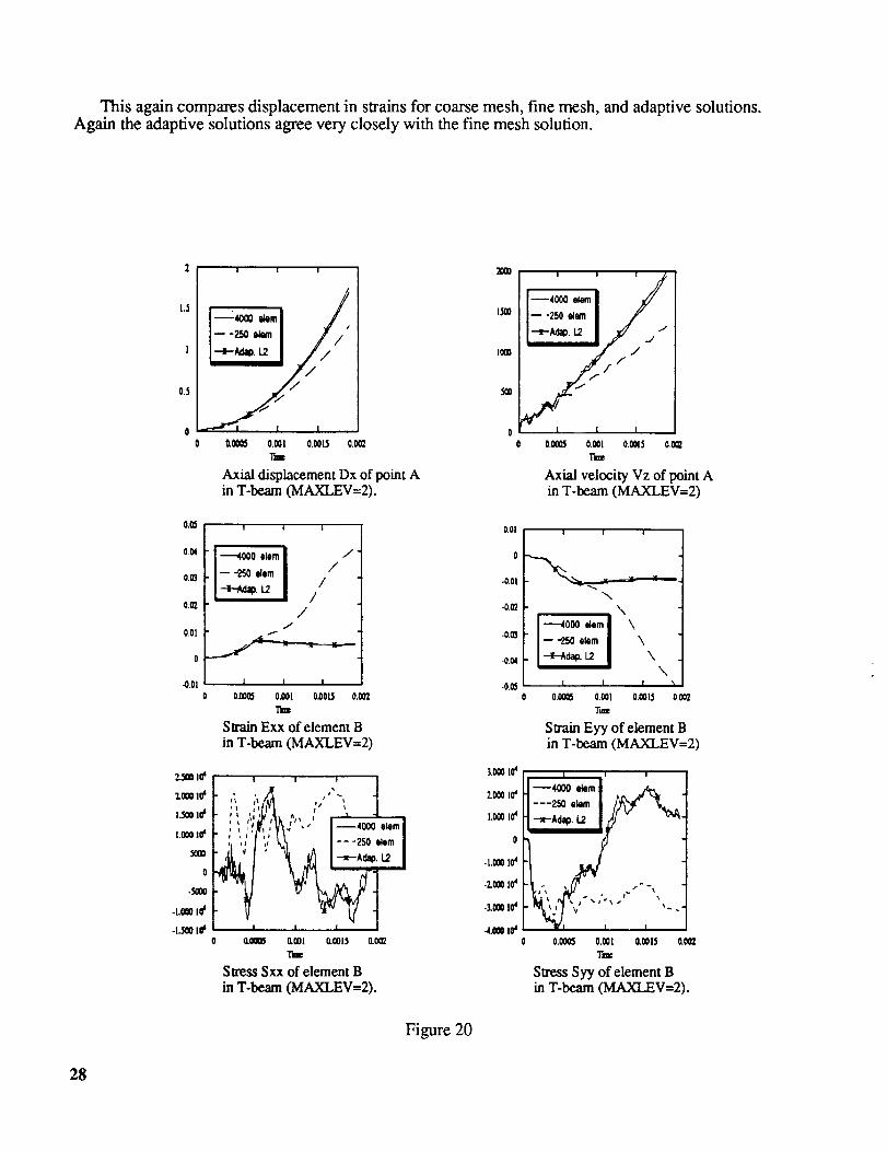
This againcomparesdisplacementin strainsfor coarsemesh,fine mesh,andadaptivesolutions.Againtheadaptivesolutionsagreeverycloselywith thefinemeshsolution.
1.5
0.5
0.05
0.04
0.0_
0.01
0
-0.01
t._ ]#
I.oc_ I#
.5OOO
0
-5(m
.]._ #
-L_ z#
| | I
i !-_" I //
0 0,00_ 0.001 0.0015 0,002T,,-
Axial displacement Dx of point Ain T-beam (MAXLEV=2).
t ! I
_000 °lem _ / /
-- "250 elem I /
"""_'_._ I //
| I I
Tk=
Strain Exx of element Bin T-beam (M_dCLEV=2)
f_
i t
t
't a_ _
,, ,/ ,,
'',; L_ I---2_ elem I
Q.OOQ5 Q,OOL (LOOTS O,002
Stress Sxx of element Bin T-_ (MAXLEV=2).
Figure 20
5®
0.01
o
-0.01
.0.02
-0.03
-0.04
.0.05
2.o00to4
z.o_oto_
o
.i.ceo 1o4
-zoo0 1o"
•iooo io4
.4._ I_
''1--25o_. I /
_Adzp, 1.2 _//.j "
/-I t I
0.00_ 0,001 O.O01_i O,OQ2
1""
Axial velocity Vz of point Ain T-beam (MAXLEV=2)
! I !
\
I -"-4000 elem I \
I- _ °"" I \
1 I I x
0.00_ 0._1 0,0015 0.002
T,-"
Strain Eyy of element Bin T-beam (MAXLEV=2)
I I !
2V ;
0.OC_ 0.0_1 I1_1_ 0.002
T_
Stress Syy of element Bin T-beam O,_v--2).
28

This is asolutionof aboxbeamwhichhasaninitial velocity asshownwith anattachedmassattheback. Thisproblemis oftenconsideredamodelfor crashanalysis.Thesolutionsfor fine mesh,coarsemeshandadaptivemeshesareShown;theadaptivesolutionagreeswell with thefinemesh.
Attachedmass,M _d wall
Beam
L
"_,
Beam Section
Geometry: L = 0.1500 ma = 0.0300 mt = 0.0015 m
Initial condition: V=15.64 m/seeMaterial number 3 (Table 6)
Box beam problem.
13.6 ._ 1--756 m"X'%
,:'>I15.55
0 0,_1 0.0_l O_ 0.0(14 O_ 0.006
Velocity of point A in the box-beam (MAXLEV=I).
-I._t$
-I.._0 I_
-7.-_ 106
.3__to*
4,_ I0"
.+._ t¢
! i ! I !
,1 t I ,
l---"° ek)mII-'--_' _' I
I ! t l l
0 n001 0.002 0.0_ 0._04 0.003 0.006
Reacdon force of box-beam (MAXLEV=I).
Figure 21
29

Thisshowsatiming for a full carmodelwhich is shownon thenextpage.It is solvedwith fullcontact-impactandsubcycling.Theimportantthingto noticeis thatsubcyclinggivesaspeedupof 1.7andthattheeffectiveelementcycletimeonaCRAY-YMPhereis 12microseconds.
Timing
FULL-CAR MODEL
Elements:
Mass (kg):
Time steps:
80 msec simulation
17,297
1,880
78,274
CRAY-YMP
Without subcycling:128 elements/block
Element cycle time:
With subcycling:64 elements/block
Effective element cycle time:
Speedup:
7.63 hrs
20 gsec
4.39 hrs
12 lasec
1.7
Figure 22
30

wlnBB - von-mises shell material - subcucle
tlme - @.BOBE+_O
Figure 23
31

wlnBB - von-mlses shell materlal - subcycle
tlme - 8.000E+00
Figure 24
32

wlnBB - von-m|ses shell materla! - subcycle
_Ime = 4._0!E+01
Figure 25
33

Implementation and Stability
Time steps are assigned to nodes and element blocks automatically.
Elements are sorted by At crite
At crit _< At2rit _< ..... _< At crite n
Elements are arranged in blocks so that time steps of adjacentelements have integer ratios.*
Blocking of elements is necessary to take advantage of vectorization.
For analysis of stability, see Belytschko and Lu, ASME publicationedited by G. Hulbert, et al, 1992.
*A new algorithm which does not require integer ratios has recentlybeen developed (Belytschko and Neal, Computer Methods inApplied Mechanics and Engineering, 31, 1989, pp. 547-570).
Figure 26
34

REMARKS AND CONCLUSIONS
• H-adaptivity is a promising technique forsimulating nonlinear structural response andstructural failure.
• Improves accuracy.
• Simplifies model preparation.
• Subcycling and advanced contact-impact methodssuch as the pinball method can improve efficiencyof explicit dynamic codes and is essentia! with h-adaptivity.
• Improved error criteria are needed for adaptivemethods for nonlinear solid mechanics.
Figure 27
35
