adaptive k-nearest neighbor classification based on a
TRANSCRIPT

Adaptive k-Nearest Neighbor ClassificationBased on a Dynamic Number of Nearest Neighbors
Stefanos Ougiaroglou1 Alexandros Nanopoulos1 Apostolos N. Papadopoulos1
Yannis Manolopoulos1 Tatjana Welzer-Druzovec2
1 Department of Informatics, Aristotle University, Thessaloniki 54124, Greece{stoug,ananopou,papadopo,manolopo}@csd.auth.gr
2 Faculty of Electrical Eng. and Computer Science, University of Maribor, [email protected]
Abstract. Classification based on k-nearest neighbors (kNN classification) isone of the most widely used classification methods. The number k of nearestneighbors used for achieving a high precision in classification is given in advanceand is highly dependent on the data set used. If the size of data set is large, thesequential or binary search of NNs is inapplicable due to the increased compu-tational costs. Therefore, indexing schemes are frequently used to speed-up theclassification process. If the required number of nearest neighbors is high, the useof an index may not be adequate to achieve high performance. In this paper, wedemonstrate that the execution of the nearest neighbor search algorithm can beinterrupted if some criteria are satisfied. This way, a decision can be made with-out the computation of all k nearest neighbors of a new object. Three differentheuristics are studied towards enhancing the nearest neighbor algorithm withan early-break capability. These heuristics aim at: (i) reducing computation andI/O costs as much as possible, and (ii) maintaining classification precision at ahigh level. Experimental results based on real-life data sets illustrate the appli-cability of the proposed method in achieving better performance than existingmethods.
Keywords: kNN classification, multidimensional data, heuristics.
1 Introduction
Classification is the data mining task [10] which constructs a model, denoted as clas-sifier, for the mapping of data to a set of predefined and non-overlapping classes. Theperformance of a classifier can be judged according to criteria such as its accuracy,scalability, robustness, and interpretability. A key factor that influences research onclassification in the data mining community (and differentiates it from classical tech-niques from other fields) is the emphasis on scalability, that is, the classifier must workon large data volumes, without the need for experts to extract appropriate samplesfor modeling. This fact poses the requirement for closer coupling of classification tech-niques with database techniques. In this paper we are interested in developing novelclassification algorithms that are accurate and scalable, which moreover can be easilyintegrated to existing database systems.
Existing classifiers are divided into two categories [12], eager and lazy. In contrast toan eager classifier (e.g., decision tree), a lazy classifier [1] builds no general model until anew sample arrives. A k-nearest neighbor (kNN) classifier [7] is a typical example of the
1
latter category. It works by searching the training set for the k nearest neighbors of thenew sample and assigns to it the most common class among its k nearest neighbors. Ingeneral, a kNN classifier has satisfactory noise-rejection properties. Other advantagesof a kNN classifier are: (i) it is analytically tractable, (ii) for k = 1 and unlimitedsamples the error rate is never worse than twice the Bayes’ rate, (iii) it is simple toimplement, and (iv) it can be easily integrated into database systems and exploit accessmethods that the latter provide in the form of indexes.
Due to the aforementioned characteristics, kNN classifiers are very popular andfind many applications. With a naive implementation, however, the kNN classificationalgorithm needs to compute all distances between training data and a testing datum,and needs additional computation to get k nearest neighbors. This negatively impactsthe scalability of the algorithm. For this reason, recent research [5] has proposed the useof high-dimensional access methods and techniques for fast computation of similarityjoins, which are available in existing database systems, to reduce the cost of searchingfrom linear to logarithmic. Nevertheless, the cost of searching the k nearest neighbors,even with a specialized access method, still increases significantly with increasing valuesof k.
For a given test datum, depending on which training data comprise its neighbor-hood, we may need a small or a large k value to determine its class. In other words,in some cases, a small k value may suffice for the classification, whereas in other caseswe may need to examine larger neighborhoods. Therefore, the appropriate k value mayvary significantly. This introduces a trade-off: By posing a global and adequately highvalue for k, we attain good accuracy, but we pay high computational cost, since asdescribed, the complexity of nearest neighbor searching increases for higher k values.Higher computational cost reduces the scalability to large data sets. In contrast, bykeeping a small k value, we get low computational cost, but this may result to loweraccuracy. What is, thus, required is an algorithm that will combine good accuracy andlow computational cost, by locally adapting the required value of k. In this work, wepropose a novel framework for a kNN classification algorithm that fulfills the aforemen-tioned property. We also examine techniques that help us for finding the appropriatek value in each case. Our contributions are summarized as follows:
– We propose a novel classification algorithm based on a non-fixed number of near-est neighbors, which is less time consuming than the known k-NN classification,without sacrificing precision.
– Three heuristics are proposed that aim at the early-break of the k-NN classificationalgorithm. This way, significant savings in computational time and I/O can beachieved.
– We apply the proposed classification scheme to large data sets, where indexing isrequired needed. A number of performance evaluation tests are conducted towardsinvestigating the computational time, the I/O time and the precision achieved bythe proposed scheme.
The rest of our work is organized as follows. The next section briefly describes re-lated work in the area and summarized our contributions. Section 3 studies in detailthe proposed early-break heuristics, and presents the modified k-NN classification al-gorithm. Performance evaluation results based on two real-life data sets are given inSection 4. Finally, Section 5 concludes out work and briefly discusses future work inthe area.
2

2 Related Work
Due to its simplicity and good performance, kNN classification has been studied thor-oughly [7]. Several variations were developed [2], like the distance-weighted kNN, whichputs emphasis on nearer neighbors, and the locally-weighted averaging, which uses ker-nel width to controls the size of neighborhood that has large effect. All such approachespropose adaptive schemes to improve the accuracy of kNN classification in the casewhere not all attributes are similar in their relevance to the classification task. In ourresearch we are interested in improving the scalability of kNN classification.
Also, kNN classification has been combined with other methods and, instead ofpredicting a class with simple voting, prediction is done by another machine learner(e.g., neural-network) [3]. Such techniques can be considered complementary to ourwork. For this reason, to keep comparison clear, we did not examine such approaches.
Bohm and Krebs [5] proposed an algorithm to compute the k-nearest neighbor joinusing the multipage index (MuX), a specialized index structure for the similarity join.Their algorithm can be applied to the problem of kNN classification and can increaseits scalability. However, it is based on a fixed number of k, which (as described inIntroduction) if it is not tuned appropriately, it can negatively impact the performanceof classification.
3 Adaptive Classification
3.1 The Basic Incremental k-NN Algorithm
An algorithm for incremental computation of nearest neighbors using the R-tree family[9, 4] has been proposed in [11]. The most important property of this method is thatthe nearest neighbors are determined in their order of their distance from the queryobject. This enables the discovery of the (k +1)-th nearest neighbor if we have alreadydetermine the previous k, in contrast to the algorithm proposed in [13] (and enhancedin [6]) which requires a fixed value of k.
The incremental nearest neighbors search algorithm maintains a priority queue. Theentries of the queue are Minimum Bounding Rectangles (MBRs) and objects which willbe examined by the algorithm and are sorted according to their distance from the querypoint. An object will be examined when it reaches the top of the queue. The algorithmbegins by inserting the root elements of the R-tree in the priority queue. Then, itselects the first entry and inserts its children. This procedure is repeated until the firstdata object reaches the top of the queue. This object is the first nearest neighbor.Figure 1 depicts the Incr-kNN algorithm with some modifications, towards adaptingthe algorithm for classification purposes. Therefore, each object of the test set is aquery point and each object of the training set, contains an additional attribute whichindicates the class where the object belongs to. The R-tree is built using the objectsof the training set.
The aim of our work is to perform classification by using a smaller number ofnearest neighbors than k if this is possible. This will reduce computational costs andI/O time. However, we do not want to harm precision (at least not significantly). Suchan early-break scheme can be applied since Incr-kNN determines the nearest neighborsin increasing distance order from the query point. The modifications performed to theoriginal incremental k-NN algorithm are summarized as follows:
3

Algorithm Incr-kNN (QueryPoint q, Integer k)1. PriorityQueue.enqueue(roots children)2. NNCounter = 03. while PriorityQueue is not empty and NNCounter ≤ k do4. element = PriorityQueue.dequeue()5. if element is an object or its MBR then6. if element is the MBR of Object and PriorityQueue is not empty
and objectDist(q, Object) > PriorityQueue.top then7. PriorityQueue.enqueue(Object, ObjectDist(q, Object))8. else9. Report element as the next nearest object (save the class of the object)10. NNCounter++11. if early-break conditions are satisfied then12. Classify the new object q in the class where the most nearest neighbors
belong to and break the while loop. q is classified usingNNCounter nearest neighbors
13. endif14. endif15. else if element is a leaf node then16. for each entry (Object, MBR) in element do17. PriorityQueue.enqueue (Object, dist(q, Object))18. endfor19. else /*non-leaf node*/20. for each entry e in element do21. PriorityQueue.enqueue(e, dist(q, e))22. endfor23. endif24. end while25. if no early-break has been performed then // use k nearest neighbors26. Find the major class (class where the most nearest neighbors belong to)27. Classify the new object q to the major class28. endif
Fig. 1. Outline of Incr-kNN algorithm with early break capability.
– We have modified line 3 of the algorithm. The algorithm accepts a maximum valueof k and is executed until either k nearest neighbors are found (no early break) orthe heuristics criteria are satisfied (early break). Specifically, we added the conditionNNCounter ≤ k in while command (line 3).
– We have added the lines 10,11,12 and 13. In this point, the algorithm retrieves anearest neighbor and checks for early break. Namely, the while loop of the algorithmbreaks if the criteria defined by the heuristic that we use are satisfied. So, the newitem is classified using NNCounter nearest neighbors, where NNCounter < k.Lines 11, 12 and 13 are replaced according to the selected heuristic.
– We have added the lines 25, 26, 27 and 28. These lines perform classification takinginto account k nearest neighbors. This code is executed only when the heuristic didnot manage to perform an early-break.
4

3.2 Early-Break Heuristics
In this section, we present three heuristics that interrupt the computation of nearestneighbors when some criteria are satisfied. The classification performance (precisionand execution cost) depends on the adjustments of the various heuristics parameters.The parameter MinnNN is common to all heuristics and defines the minimum num-ber of nearest neighbors which must be used for classification. After the retrieval ofMinnNN nearest neighbors, the check for early-break is performed. The reason forthe use of MinNN is that a classification decision is preferable when it is based ona minimum number of nearest neighbors, otherwise precision will be probably poor.These criteria depend on which proposed heuristic is used. The code of each heuristicreplaces lines 11 and 12 of the Incr-kNN algorithm depicted in Figure 1.
Simple Heuristic (SH) The first proposed heuristic is very simple. According to thissimple heuristic, the early-break is performed when the percentage of nearest neighborsthat vote the major class is greater than a predefined threshold. We call this thresholdPMaj.
For example, suppose that we have a data set where the best precision is achievedusing 100 nearest neighbors. Also, suppose that we define that PMaj = 0.9 andMinNN=7. The Incr-kNN is interrupted when 90% of NNs vote a specific class. Ifthis percentage is achieved when the algorithm examines the tenth NN (9 out of 10NNs vote a specific class), then we avoid the cost of searching the rest 90 nearest neigh-bors. Using the Incr-kNN algorithm, we ensure that the first ten neighbors which havebeen examined, are the nearest.
Furthermore, if the simple heuristic fails to interrupt the algorithm because PMaj isnot achieved, it will retry an early-break after finding the next TStep nearest neighbors.
Independent Class Heuristic (ICH) The second early-break heuristic is the In-dependent Class Heuristic (ICH). This heuristic does not use the PMaj parameter.The early-break of Incr-kNN is based on the superiority of the major class. Superiorityis determined by the difference between the sum of votes of the major class and thesum of votes of all the other classes. The parameter IndFactor (Independency Factor)defines the superiority level of the major class that must be met in order to perform anearly-break. More formally, in order to apply an early-break, the following conditionmust be satisfied:
SV MC > IndFactor ·n∑
i=1
SV Ci − SV MC (1)
where SV MC is the sum of votes of major class, n is the number of classes and SV Ci
is the sum of votes of class i.For example, suppose that our data set contains objects of five classes, we have
set IndFactor to 1 and the algorithm has determined 100 NNs. Incr-kNN will beinterrupted if 51 NNs vote a specific class and the rest 49 NNs vote the other classes. Ifthe value of IndFactor is set to 2, then the early-break is performed when the majorclass has more than 66 votes.
Studying the Independent Class Heuristic, we conclude that the value of the IndFactorparameter should be adjusted by taking into account the number of classes and the
5
class distribution of data set. In the case of a normal distribution, we accept the follow-ing rule: when the number of classes is low, IndFactor should be set to a high value.On the other hand, when there are many classes, IndFactor should be set to a lowervalue.
In ICH, parameter TStep is used in the same way as in the SH heuristic. Specifically,when there is a failure in interruption, the early-break check is again activated afterdetermining the next TStep nearest neighbors.
M-times Major Class Heuristic (MMCH) The last heuristic that we present istermed M-Times Major Class Heuristic (MMCH). The basic idea is to stop the Incr-kNN when M consecutive nearest neighbors, which vote the major class, are found.In other words, the while-loop of Incr-kNN algorithm terminates when the followingsequence of nearest neighbors appears:
NNx+1, NNx+2, ..., NNx+M ∈ MajorClass (2)
However, this sequence is not enough to for an early-break. In addition, the PMajparameter is used in the same way as in the SH heuristic. Therefore, MMCH heuristicbreaks the while loop when the percentage of nearest neighbors that vote the majorclass is greater than PMaj and there is a sequence of M nearest neighbors that belongto the major class. We note that MMCH does not require the TStep parameter.
4 Performance Evaluation
In this section, we present the experimental results on two real-life data sets. All exper-iments have been conducted on an AMD Athlon 3000+ machine (2000 MHz), with 512MB of main memory, running Windows XP Pro. The R*-tree, the incremental kNNalgorithm, and the classification heuristics have been implemented in C++.
4.1 Data Sets
The first data set is the Pages Blocks Classification (PBC) data set and contains 5,473items. Each item is described by 10 attributes and one class attribute. We have usedthe first five attributes of the data set and the class attribute. We reduced the numberof attributes considering that the most dimensions we use, the worst performance thefamily of R-trees has. Each item of the data set belongs to one of the five classes.Furthermore, we have divided the data set into two subsets. The first subset contains4,322 items used for training and the second contains the rest 1,150 items used fortesting purposes.
The traditional kNN classification method achieves the best possible precision whenk = 9. However, this value was very low and so the proposed heuristics can not revealtheir full potential. Therefore, we have added noise in the data set in order to makethe use of a higher k value necessary. Particularly, for each item of the train set, wemodified the value of the class attribute with probability 0.7 (the most noise is added,the highest value of k is needed to achieve the best classification precision). This factforced the algorithm to use a higher k value. This way, we constructed a data set wherethe best k value is 48. This means that the highest precision value is achieved when 48nearest neighbors contribute to the voting process. This is illustrated in Figure 2(a),which depicts the precision value accomplished by modifying k between 1 and 48.
6

�
����
����
����
����
����
����
���
� � � � � � �� �� �� �� ��
����������
��� ���
�
�
�
�
�
�
�
��
��
� � � �� �� ��
����������
���
�
����
����
����
����
����
����
���
� � � � � � ��
���
��� ���
�
� �������
�
� �������
���
���
��� ��� ���
Fig. 2. Precision vs k, I/O vs k and precision vs I/O for PBC data set.
��� ��� ���
�
����
���
���
����
����
���
����
����
����
� � �
����������
��� ���
�
����
���
����
���
�����
� ���
�����
� ���
� � �
����������
���
�
����
���
���
����
����
���
����
����
���� ���� ���� ���� ����� �����
���
��� ���
���������
� �
���������
���
���
Fig. 3. Precision vs k, I/O vs k and precision vs I/O for LRI data set.
As expected, the higher the value of k, the higher the number of I/O operations.This phenomenon is illustrated by Figure 2(b). We note that if we had used a lowervalue for k (k ¡ 48), we would have avoided a significant number of I/Os and thereforethe search procedure would be less time-consuming. For example, if we set k = 30, thenwe avoid 5.84 I/Os for the classification of one item of the test set without significantimpact on precision. Figure 2(c) combines the two previous graphs. Particularly, thisfigure shows how many I/Os the algorithm requires in order to accomplish a specificprecision value.
The second data set is the Letter Image Recognition Data set [8], which contains20,000 items. We have used 15,000 items for training and 5,000 items for testing. Eachitem is described by 17 attributes (one of them is the class attribute) and represents animage of a capital letter of the English alphabet. Therefore, the data set has 26 classes(one for each letter). The data set objective is to identify the capital letter representedby the items of the test set using a classification method.
As in the case of the PBC data set, we have reduced the number of dimensions(attributes). In this case, dimensionality reduction has been performed by using Prin-cipal Component Analysis (PCA) on the 67% of the original data. The final numberof dimensions have been set to 5 (plus the class attribute).
Figure 3 illustrates the data set behavior. Specifically, Figure 3(a) shows the preci-sion achieved for k ranging between 1 and 28. We notice that the best precision (77%)is achieved when k = 28. Figure 3(b) presents the impact of k on the number of I/Os.Almost 43 I/O operations are required to classify an item of the test set for k = 28.Finally, Figure 3(c) combines the two previous graphs illustrating the relation betweenprecision and the number of I/O operations. By observing these figures, we concludethat if we had used a lower k value, then we could have achieved better execution timeby keeping precision at high levels.
7

4.2 Determining Parameters Values
Each heuristic uses a number of parameters. These parameters must be adjusted sothat the best performance is achieved (or the best balance between precision and exe-cution time). In this section, we present a series of experiments which demonstrates thebehavior of the heuristics for different values of the parameters. We keep the best val-ues (e.g. the parameters that manage to balance execution time and precision) for eachheuristic and use these values in a subsequent section where heuristics are compared.
Pages Blocks Classification Data Set Initially, we are going to analyze the MinNNparameter. It is a parameter that all heuristics use. Recall that MinNN is the min-imum number of NNs that should be used for classification. After determining theseNNs, the heuristics are activated. Figure 4 show how the heuristics performance (pre-cision and I/O) is affected by modifying the value of MinNN . The values of the otherparameters have as follows: TStep = 4, IndFactor = 1, PMaj = 0.6, MTimes = 4,k = 48.
����
����
����
����
����
����
����
� � � � � �� �� �� �� � ��
�����������
� ������
� ��������� �� � �� �������� �� �
���������������������� �� � !!������ " ��� #�
��
��
��
��
��
��
��
��
��
��
��
� � � � � �� �� �� �� � �������������
���
� ��������� �� � �� �������� �� �
���������������������� �� � !!������ " ��� #�
����� �����
Fig. 4. Impact of MinNN for PBC data set.
By observing the results it is evident that precision is least affected when the MMCHheuristic is used. Therefore, for this heuristic, we set MinNN = 4, which is the valuethat provides the best balance between I/O and precision. In contrast, the precision ofthe other two heuristics is significantly affected by the increase of MinNN . We decideto define MinNN = 11 for the Independency Class Heuristic and MinNN = 7 forthe Simple Heuristic. Our decision is justified by the precision and I/O measurementsprovided for these parameters values.
We continue our experiments by finding the best value for IndFactor. Recall thatthis parameter is used only in ICH heuristic. We modify IndepFactor from 0.4 to 4and calculate the precision achieved. Figure 5 illustrates that the best balance betweenprecision and I/O is achieved when IndFactor = 1. The values of the other parametersare as follows: MinNN = 11, TStep = 4, k = 48.
Next we study the impact of the parameter MTimes, which is used only by theMMCH heuristic. As it is depicted in Figure 6 for MTimes = 3, the precision levelwill be high enough and the number of I/O operations is relatively low. So we keepthis value as the best possible for this parameter. The values of the other parametershave as follows: MinNN = 4, PMaj = 0.6, k = 48.
8

����
����
����
����
����
����
��� �� ��� � �� ��� �� ��� � �� � �� � �� ��� �� ��� �
��������
��� ���
� ���� �� �����������������
��
�
��
�
�
�
��
�
��� �� ��� � �� ��� �� ��� � �� � �� � �� ��� �� ��� �
��������
���
� ���� �� �����������������
�������� ��������
Fig. 5. Impact of IndFactor on the performance of ICH heuristic for PBC data set.
�����
�����
�����
�����
�����
�����
�����
�����
�����
�����
����
� � � � � � �� �� ��
�����������
� �������
� ��������������
�
��
��
��
��
��
��
� � � � � � �� �� ��
�����������
���
� ��������������
������������
Fig. 6. Impact of MTimes on the performance of MMCH heuristic for PBC data set.
Next, we study the impact of TStep parameter on the performance of SC and ICH,since MMCH does not use this parameter. Figure 7 depicts the results. The values ofthe rest of the parameters have as follows: MinNN = 6, IndFactor = 1, PMaj = 0.6,MTimes = 3, k = 48. Both SH and ICH heuristics achieve the best precision whenTStep = 4. In fact, SH achieves the same precision for TStep = 3 or TStep = 4, butless I/Os are required when TStep = 4. Since MMCH and kNN classification are notaffected by TStep, their graphs are parallel to the TStep axis. Finally, it is worth tonote that although MMCH needs significantly less I/Os than kNN classification, theprecision that MMCH achieves is the same as that of kNN classification.
Letter Image Recognition Data Set Next, we repeat the same experiments usingthe LIR data set. The impact of MinNN is given in Figure 8. It is evident that allheuristics achieve higher precision than kNN classification. By studying Figure 8 wedetermine that the best MinNN values for the three heuristics are: MinNN = 7 forSH, MinNN = 12 for ICH and MinNN = 4 for MMCH. These values achieve thebest balance between precision and I/O processes. The values of the other parametershave as follows: TStep = 2, IndFactor = 1, PMaj = 0.6, MTimes = 3, k = 28.
Figure 9 depicts the results for the impact of IndFactor. We see that IndFactor =1 is the best value since the ICH heuristic achieve the best possible precision value andat the same time saves almost ten I/O operations per query. The values of the otherparameters are as follows: MinNN = 12, TStep = 5, k = 28.
Next, we consider parameter MTimes, which is used only by the MMCH heuristic.We define MTimes = 3, which results in 13 I/O savings for each query and achieves
9

����
�����
����
�����
����
�����
����
�����
����
�����
� � � � � �� �������������
��������
�� ������������� ��� ������������
��������������������� ������ ���!�� ��"�
��
��
��
�#
��
��
��
��
� � � � � �� ������� ���� �
���
�� ������������� ��� ������������
��������������������� ������ ���!�� ��"�
����������
Fig. 7. Impact of TStep parameter for PBC data set.
����
����
����
����
����
����
����
����
� � � � � �� �� �� �� � ��
�����������
� ������
� ��������� �� � �� �������� �� �
���������������������� �� � !!������ " ��� #�
��
�
��
�
��
� � � � � �� �� �� �� � ��
�����������
���
� ��������� �� � �� �������� �� �
���������������������� �� � !!������ " ��� #�
����� �����
Fig. 8. Impact of MinNN for LIR data set.
������������������ ������
����
����
����
����
����
����
����
��� ��� ��� � ��� ��� ��� ��� � ��� ��� ��� ��� � ��� ��� ��� ��� �
��������
��� ���
������������������ ������
������������������ ������
��
��
��
��
��
��
��
��
��
��
��� ��� ��� � ��� ��� ��� ��� � ��� ��� ��� ��� � ��� ��� ��� ��� �
��������
���
������������������ ������
�������� ��������
Fig. 9. Impact of IndFactor on the performance of ICH heuristic for LIR data set.
the best possible precision value. The results are illustrated in Figure 10. The valuesof the other parameters have as follows: MinNN = 4, PMaj = 0.6, k = 28.
Finally, in Figure 11 we give the impact of TStep. We set TStep = 4 for SH andTStep = 5 for ICH, since these values give adequate precision and execution time. Thevalues of the rest of the parameters have as follows: MinNN = 4, IndFactor = 1,PMaj = 0.6, MTimes = 3, k = 28.
10

�����
�����
�����
�����
�����
�����
� � � � � � �� �� ��
�����������
� �������
� ��������������
��
�
��
��
�
��
�
� � � � � � �� �� ��
�����������
���
� ��������������
������ ������
Fig. 10. Impact of MTimes on the performance of MMCH heuristic for LIR data set.
����
����
����
����
����
����
����
����
� � � � � � ������������
��������
� ��������� �� � �� �������� �� �
���������������� �� � ���� �!�� " �!� #�
�
�
��
��
�
�
� � � � � � ������ �����
���
� ��������� �� � �� �������� �� �
���������������� �� � ���� �!�� " �!� #�
����� �����
Fig. 11. Impact of TStep parameter for LIR data set.
4.3 Comparison of Heuristics
In this section we study how the heuristics compare to each other and to the traditionalkNN classification, by setting the parameters to the best values for each heuristic, asthey have been determined in the previous section.
Pages Blocks Classification Data Set Figure 12 depicts the performance results vsPMaj. When PMaj = 0.6, precision is about the same for all heuristics and very closeto that achieved by traditional kNN classification. However, our heuristics require sig-nificant less I/O for achieving this precision. When this precision value is accomplishedthere is no reason to find more nearest neighbors and therefore valuable computationalsavings are achieved.
According to our results, ICH achieves a precision value of 0.947 (kNN’s precisionis 0.9495) while it saves about 6.88 I/Os for the classification of one item. Particularly,when we use ICH, we find 31.29 nearest neighbors on average instead of 48. Similarly,when PMaj = 0.6, SH achieves precision equal to 0.948 (very close to that of kNN)by performing an early-break when 38.5 NNs on average have been found (almost 10less than kNN requires). Therefore, SH saves about 4.385 I/Os per each item of thetest set. Finally, the same precision value (0.948) is achieved by MMCH. However, thisheuristic saves less number of I/Os than SH. Specifically, MMCH spends 3.875 I/O lessthan kNN because it finds 39.767 NNs on average.
Figures 13 and 14 summarize the results of this experiment using bar charts whichhave been produced by setting PMaj = 0.6 and maintain the same values for the otherparameters. Figure 13 shows that the precision achieved by the heuristics is very closeto that of kNN, whereas the number of required I/Os is significant less than that of
11

����
����
����
����
����
����
�� ��� �� ��� ��� ��� ���
����������
� �������
�� ������������� ��� ��������������������������������������� ���� �����!�����"�
��
��
��
#�
#$
#�
#�
#�
$�
$$
$�
�� ��� �� ��� ��� ��� ���
����������
���
�� ������������� ��� ������������
������������ �������������� ���� �����!�����"�
��������
Fig. 12. Precision and number of I/Os.
����������� ��
������ ��� ��� �
���������� ��������
���� �� ��������� ��� �� ���
� ������
� ������
� ������
� ������
� ������
� ������
� ������
���������
������ ��� ��� � ������ ��� ��� � ����������� ������ ��� ��� � �������� ���� �� ���
���� �� ��� ��� � ������ ������ �
����������� ����� ��
����� �
������������ �� ���
�
�
�
!
��
�
��
�
������ ����� � � ����������� �� ����������� ������ ��� ��� � ��������� ��� �� ���
Fig. 13. Precision and number of I/Os for PMaj = 0.6
������ ������� ������ �������
����������� ������ �
����� �
������������ �����
��
��
��
��
��
��
��
��������������
������������� ������������� ����������� ������ ������� ��������� ��� �����
Fig. 14. Required number of nearest neighbors for PMaj = 0.6.
kNN. Figure 14 presents the number of nearest neighbors retrieved on average by eachmethod.
We can not directly answer the question which heuristic is the best. The answer de-pends on which measure is more critical (precision or execution time). If a compromisemust be made, Figure 12 will help. We notice that ICH shows the best performancebecause it achieves a precision that is very close to the precision of kNN posing theminimum number of I/Os. To declare a winner between SH and MMCH we notice thatwhen PMaj > 0.6 the heuristics achieves almost the same precision, but MMCH posesmore I/Os than SH.
As we have already mentioned, we try to find the parameters values that provide acompromise between precision and execution time. However, if one of these measuresis more important than the other, the parameters can be adjusted to reflect this pref-erence. Suppose that execution time is more critical than precision (when for example
12

a quick-and-dirty scheme should be applied due to application requirements). If we sePMaj = 0.5, then 23.245 I/Os per query will be required (instead of 33.32 requiredby kNN) by finding 25.72 NNs instead of 48. However, this means that precision willbe significantly smaller than that of kNN (we saw that when PMaj = 0.6, the differ-ence between the precision of SH and kNN is minor). Similar results are obtained forMMCH when PMaj = 0.5. On the other hand, if precision is more critical than time,we can adjust the heuristics parameters towards taking this criticality into account. Inthis case, it is possible that the heuristics achieve better precision than kNN, with exe-cution time overhead. In any case, early-break heuristics always require less executiontime than kNN.
By considering the impact of MinNN shown in Figure 4, it is evident that MMCHcan achieve a slightly better precision than kNN. Specifically, if we set MinNN =8, PMaj = 0.6 and MTimes = 3, then MMCH achieves a precision value equal to0.950435, whereas 30.793 I/Os are required (while kNN requires 33.3174 I/Os per queryand achieves a precision of 0.94956). The early-break heuristic is able to avoid 2.5244I/O per query, whereas at the same time achieves better precision when k is adjustedto ensure the best precision value. Although the number of saved I/Os may seemssmall, note that this savings are performed per classified item. Since the PBC test setcontains 1,150 items, we realize that the overall number of saved I/Os is 2903, whichis significant.
Similar considerations apply to the other two heuristics. For example, ICH canoutperform the precision of kNN when IndyFactor = 1.2, TStep = 4, and MinNN= 11 (see Figure 5). However, because of the increase of IndFactor from 1 to 1.2, theI/O requirements are increased from 26.44 to 29.75. Finally, if we set MinNN = 11
����������� �� ����������� ��
���������������� ��
����� � ���������� �� � ����
� ����
� ����
� ����
� ����
� ���
� ����
���������
���� �� ������ � ������������� ����������������� ������ � ��������� ��� �����
������������ �
������ ������ �
������������ �����
������������������
����� �
!�
!"
!�
�
�
!
�
�
������������ � ������������� ����������������� ������ � ��������� ��� �����
Fig. 15. Precision and number of I/Os (MinNN = 11).
�������������
�������������
������������ �����
������������������
������
��
��
��
��
��
��
��
��
��
��
��
��������
������������� ������������� ������������������������ ������������ �����
Fig. 16. Required number of nearest neighbors (MinNN = 11).
13
instead of 7, SH also outperforms the precision of kNN (see Figure 4). These resultsare illustrated in Figures 15 and 16.
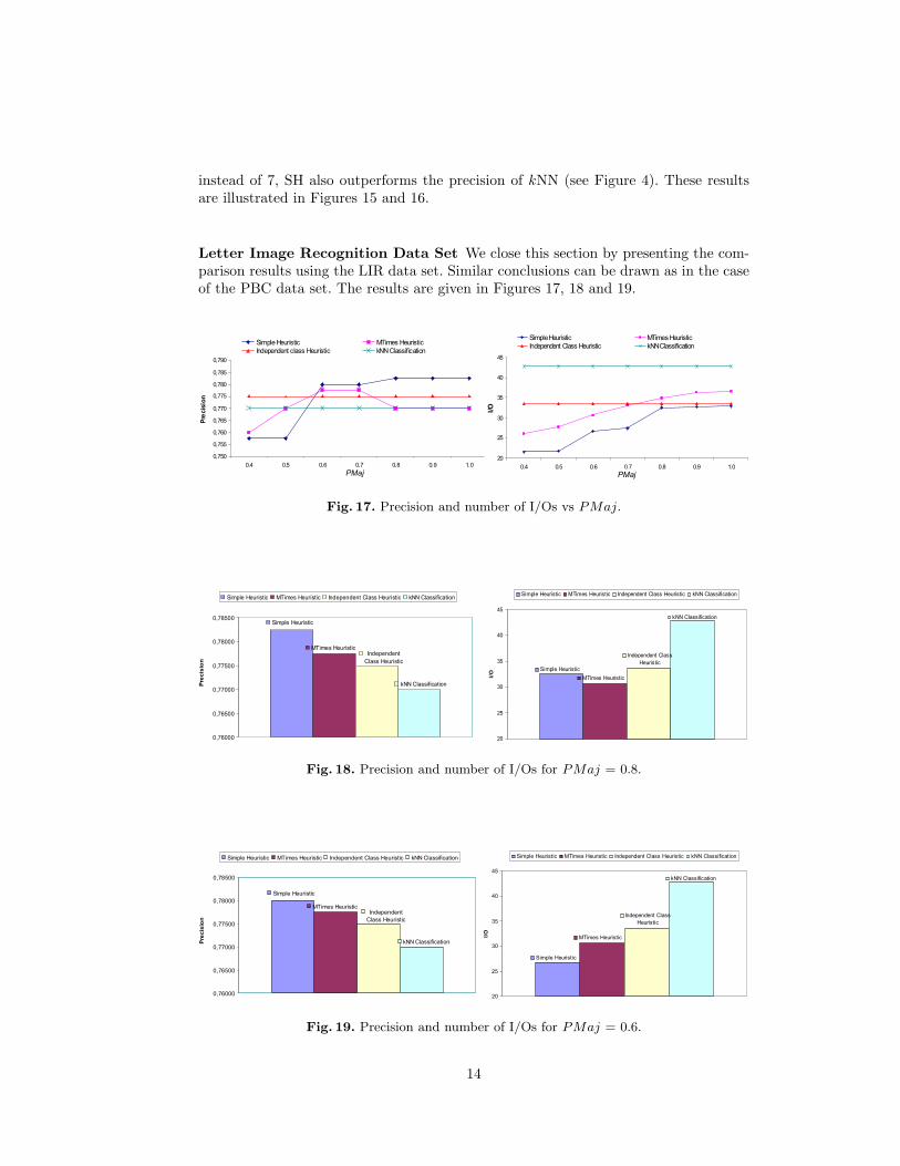
Letter Image Recognition Data Set We close this section by presenting the com-parison results using the LIR data set. Similar conclusions can be drawn as in the caseof the PBC data set. The results are given in Figures 17, 18 and 19.
�����
�����
�����
�����
�����
�����
�����
�����
�����
�� ��� ��� ��� ��� ��� ��
����������
� �������
�� ������������� ��� ������������
��������������������������� ���� �����!�����"�
#�
#�
$�
$�
�
�
�� ��� ��� ��� ��� ��� ������������
���
�� ������������� ��� ������������
������������ �������������� ���� �����!�����"�
���� ����
Fig. 17. Precision and number of I/Os vs PMaj.
�
�������������
������������� ������������
������������
������������ �����
�������
�������
�������
�������
�������
�������
���������
������������� ������������� ������������������������ ������������ ������
�������������
�������������
������������������
������
������������ �����
��
��
�
�
!�
!�
�
������������� ������������� ������������������������ ������������ �����
Fig. 18. Precision and number of I/Os for PMaj = 0.8.
�
�������������
������������� ������������
������������
������������ �����
�������
�������
�������
�������
�������
�������
���������
������������� ������������� ������������������������ ������������ ����� �
�������������
�������������
������������������
������
������������ �����
��
��
�
�
!�
!�
�
������������� ������������� ������������������������ ������������ �����
Fig. 19. Precision and number of I/Os for PMaj = 0.6.
14
We note that when we PMaj > 0.5 (see Figure 17), the three heuristics accomplishbetter precision than kNN and manage to reduce execution time. More specifically, SHachieves a precision of 0.7825 with 32.53 I/Os on average for PMaj = 0.8, whereaskNN a precision of 0.77 spending 42.81 I/Os (see Figure 18). Also, if we set PMaj =0.6, SH achieves a precision of 0.78 spending 26.7775 I/Os on average (see Figure 19).
ICH, which is not affected by the PMaj parameter, achieves a precision of 0.775spending 33.52745 I/Os on average. Finally, MMCH achieves the best balance be-tween precision and execution time we set PMaj = 0.6. Particularly, the heuristicaccomplishes a precision of 0.7775 and spends 30.6525 I/Os on average (see Figure18). Comparing the three heuristics using the Letter Image Recognition data set, weconclude that the simple heuristic has the best performance since it achieves the bestpossible precision spending the least possible number of I/Os.
5 ConclusionsIn this paper, an adaptive kNN classification algorithm has been proposed, which doesnot require a fixed value for the required number of nearest neighbors. This is achievedby incorporating an early-break heuristic into the incremental k-nearest neighbor algo-rithm. Three early-break heuristics have been proposed and studied, which use differentconditions to enforce an early-break. Performance evaluation results based on two real-life data sets have shown that significant performance improvement may be achieved,whereas at the same time precision is not reduced significantly (in some cases pre-cision is even better than that of kNN classification). We plan to extend our worktowards: (i) incorporating more early-break heuristics and (ii) studying incrementalkNN classification by using subsets of dimensions instead of the whole dimensionality.
References
1. D. W. Aha. Editorial. Artificial Intelligence Review (Special Issue on Lazy Learning),11(1-5):1–6, 1997.
2. C. Atkeson, A. Moore, and S. Schaal. Locally weighted learning. Artificial IntelligenceReview, 11(1-5):11–73, 1997.
3. C. Atkeson and S. Schaal. Memory-based neural networks for robot learning. Neurocom-puting, 9:243–269, 1995.
4. N. Beckmann, H.-P. Kriegel, R. Schneider, and B. Seeger. The r*-tree: An efficient androbust access method for points and rectangles. In Proceedings of the ACM SIGMODConference, pages 590–601, 1990.
5. C. Boehm and F. Krebs. The k-nearest neighbour join: Turbo charging the kdd process.Knowledge and Information Systems, 6(6):728–749, 2004.
6. K.L. Cheung and A. Fu. Enhanced nearest neighbour search on the r-tree. ACM SIGMODRecord, 27(3):16–21, 1998.
7. B.V. Dasarathy. Nearest Neighbor Norms: NN Pattern Classification Techniques. IEEEComputer Society Press, 1991.
8. P.W. Frey and D.J. Slate. Letter recognition using holland-style adaptive classifiers.Machine Learning, 6(2):161–182, 1991.
9. A. Guttman. R-trees: A dynamic index structure for special searching. In Proceedings ofthe ACM SIGMOD Conference, pages 47–57, 1984.
10. J. Han and M. Kamber. Data Mining: Concepts and Techniques. Morgan Kaufmann,2000.
11. G.R. Hjaltason and H. Samet. Distance browsing in spatial databases. ACM Transactionson Database Systems, 24(2):265–318, 1999.
12. M. James. Classification Algorithms. John Wiley & Sons, 1985.13. N. Rousopoulos, S. Kelley, and F. Vincent. Nearest neigbor queries. In Proceedings of the
ACM SIGMOD Conference, pages 71–79, 1995.
15