adaptive fuzzy sliding mode controller for the kinematic ... · adaptive fuzzy sliding mode...

UNMANNED SYSTEMS PAPER

Adaptive Fuzzy Sliding Mode Controller for the KinematicVariables of an Underwater Vehicle

Eduardo Sebastián & Miguel A. Sotelo

Received: 3 August 2006 /Accepted: 27 January 2007 /Published online: 24 March 2007# Springer Science + Business Media B.V. 2007

Abstract This paper address the kinematic variables control problem for the low-speedmanoeuvring of a low cost and underactuated underwater vehicle. Control of underwatervehicles is not simple, mainly due to the non-linear and coupled character of systemequations, the lack of a precise model of vehicle dynamics and parameters, as well as theappearance of internal and external perturbations. The proposed methodology is anapproach included in the control areas of non-linear feedback linearization, model-basedand uncertainties consideration, making use of a pioneering algorithm in underwatervehicles. It is based on the fusion of a sliding mode controller and an adaptive fuzzysystem, including the advantages of both systems. The main advantage of this methodologyis that it relaxes the required knowledge of vehicle model, reducing the cost of its design.The described controller is part of a modular and simple 2D guidance and controlarchitecture. The controller makes use of a semi-decoupled non-linear plant model of theSnorkel vehicle and it is compounded by three independent controllers, each one for thethree controllable DOFs of the vehicle. The experimental results demonstrate the goodperformance of the proposed controller, within the constraints of the sensorial system andthe uncertainty of vehicle theoretical models.

Keywords Adaptive equalization . Fuzzy models and estimators . Marine systems .

Non-linear control . Robots dynamics . Sliding mode control

1 Introduction

Underwater vehicles have replaced human beings, in a great number of scenarios,especially in dangerous or precise tasks. Scientific and technological tasks, such as

J Intell Robot Syst (2007) 49:189–215DOI 10.1007/s10846-007-9144-y

E. Sebastián (*)Centro de Astrobiología (CAB), Laboratorio de Robótica y Exploración Planetaria,Ctra. Ajalvir Km. 4. Torrejón de Ardoz, Madrid, Spaine-mail: [email protected]

M. A. SoteloDepartamento de Electrónica, Universidad de Alcalá, N-II Km. 33. Alcalá de Henares, Madrid, Spain

underwater cave exploration, automatic sample recovery or cable and pipe inspection, makethe design of automatic navigation and control systems necessary, giving the robotprecision and autonomy. Even though the problem of underwater vehicle control isstructurally similar to the control of a rigid body of six degrees of freedom (DOF), widelystudied in the literature, it is more difficult because of the unknown non-linearhydrodynamic effects, parameter uncertainties, internal and external perturbations such uswater current or sideslip effect.

The problem analysed in this paper, the low-speed control of the kinematic variables ofan underactuated underwater vehicle, can be defined as follows. Given an unknownunderwater vehicle plant and a continuous bounded time-varying velocity and/or positionreferences, how to design a controller that ensures that the plant state convergesasymptotically to the kinematic references. The designed controller is part of a controland guidance architecture, and it receives input references from the guidance system thatensures the tracking of the trajectory.

Most dynamically positioned marine vehicles in used today employ PI or PID controllersfor each kinematic variable. These controllers are designed based on the assumption that theplant is a second order linear time invariant dynamical system, and that the disturbanceterms of hydrodynamics forces, water currents and wind are constant. Additionally, theyprovide theoretically set point regulation if disturbances are constant, using Lasalle’sInvariance Theorem, while they can not provide exact tracking even for linear plant [7].Moreover, PID control can not dynamically compensate for unmodeled vehicle hydrody-namic forces or unknown variations in disturbances like current and wind. To avoid thisproblem only a reduced number of commercial vehicles employ model-based compensationof hydrodynamic terms and desired acceleration. The reason why these controllers are notwidely used is that the required plant model is unavailable and the associated plantparameters are difficult to estimate with any accuracy, consequencely in practice they areempirically tuned by trial and error.

From this point of view, most of the proposed control schemes take into account theuncertainty in the model by resorting to an adaptive strategy or a robust approach. Asignificant number of studies have employed linearized plant approximations [13], in orderto apply linear control techniques. In [18], a linear discrete time approximation for vehicledynamics is used with reported numerical simulations of linear square and robust controlmethods. In [23] the author reports self-tuning control of linearized plant models andnumerical simulations. In [20] the authors report linear model-reference adaptive control oflinearized plant model and experimental demonstrations. In [19] the authors report thesliding-mode control of a linearized plant models and numerical simulations.

In the area of non-linear and modern control, relatively few studies directly addresssemi-decoupled non-linear plant models for underwater vehicles. In [33] the authors reportnon-linear sliding mode control for surge, sway and yaw movements. The most attractivecharacteristic of the sliding control is its inherent robustness to model uncertainties,obtained from an important control effort. Also, adaptive versions of sliding controllershave been implemented [10, 32], effectively reducing model uncertainty and controlactivity, and maintaining robustness without sacrificing performance. In [27] the authorscompare, using experimental trial, some of the previously reported controllers, based on adecoupled non-linear plant model of the JHUROV vehicle.

Other techniques, besides sliding control have been used in UUV, in [16] a statelinearization control is studied. However, this control technique can only be applied whenthe model of the system and its parameters are known. A step forward in the design ofcontrollers with feedback linearization derives from the capacity to adapt the values of the

190 J Intell Robot Syst (2007) 49:189–215

model parameters, supposing the model is known. In [9] an adaptive non-linear controller[26] has been tested, showing a practical implementation of a MIMO controller for theautonomous underwater vehicle AUV ODIN. One of the problems that this control lawpresents is the sensitivity to noise in the measurement of the kinematic variables. In [15] amodification of the non-linear adaptive control law is presented, in which during theprocess of adaptation the velocity and position measurements are replaced by their inputreferences.

Several studies address fully coupled non-linear plant models and controllers [3, 4, 6]and [14]. In [21] a sliding control is used to stabilize the vehicle in a straight trajectory,considering model uncertainty and external perturbations. Other authors [1, 2] have takeninto account the dynamics of the vehicle, for which they introduce the curvature of thetrajectory like a new state variable. Lastly, in [12] the author gives a solution to the problemof the internal perturbations like the sideslip effect, or external like water currents,proposing an integrated methodology of guidance and control. For this, backsteppingtechniques are used which give a recursive design frame, guaranteeing the global stabilityby Lyapunov theory and accounting for the water currents by their estimation. Some ofthese approaches typically make explicit assumptions on the structure of the approximatevehicle plant dynamics to ensure that the vehicle plant model possesses passivity propertiesidentical to those possessed by rigid-body holonomic mechanical systems, an assumptionthat has not been widely empirically validated for low speed underwater vehicles. In spiteof that, the design of a unique controller for all the DOF of an underwater vehicle, in orderto be part of a trajectory following system, is an area of research, still open [35]. At present,the motion and force control of the system vehicle-manipulator is one of the most activeareas of research [5].

In the area of intelligent control, different controllers have been designed. For example,in [34] a neural control is proposed, using an adaptive recursive algorithm of which theprincipal characteristic is the on-line capability of adjustment, without having an implicitmodel of the vehicle, due to author employed nonparametric control methodologies that donot require knowledge of the plant dynamics. It has been tested with success in the ODINvehicle. Finally, [11] proposes a fuzzy controller with 14 rules for depth control of an AUV.

This paper studies a kinematic variables controller, making use of a pioneering algorithmin underwater vehicles, which is based on the work and results developed in [31], aboutadaptive fuzzy sliding mode control (AFSM). The controller uses Euler angles and body fixreference frame to describe a semi-decoupled non-linear plant model of the underactuatedSnorkel vehicle, that it is compounded by three independent controllers, each one for thecontrollable DOF. The methodology is an approach focused in the field of affine non-linearsystems, based on uncertainty considerations, and model-based approximation of non-linearfunctions and feedback linearization with neural networks and fuzzy logic, [17] and [30].The controller is based on the fusion of a sliding mode controller and an adaptive fuzzysystem, adaptive exhibits and robust features. The adaptive capabilities are provided byseveral fuzzy estimators, while robustness is provided by the sliding control law, showingthe advantages of both systems. But one of the main advantages of the proposed theory isthat it employs a nonparametric adaptive technique which requires a minimum knowledgeof plant dynamics, only needing a theoretical and simple model. A Lyapunov-like stabilityanalysis of the control algorithm is described. The algorithm is also based on the analysisdeveloped in [31], which has been adapted to the peculiarities of the vehicle model, withsome changes. The stability analysis ensures the stability of the adaptation process and theconvergence to the references. The resulting control law is validated in practicalexperiments for controlling the Snorkel, carried out for the first time in this work, by a

J Intell Robot Syst (2007) 49:189–215 191

UUV developed at the Centro de Astrobilogía. The most important characteristic of thevehicle is the low cost of all instruments and methods used in the design, conditioning andlimiting the identification experiments.

Additionally, the paper reports a direct comparison of the performance of the AFSMcontroller with more simple control schemes like sliding mode controller (SM) or a velocityPI controller, based on a theoretical plant model and investigating the effects of bad modelparameters on system tracking performance. Practical aspects of the implementation arealso discussed. The experimental results obtained demonstrate the good performance of theproposed controller, outperforming more simple ones.

The paper is organized as follows; Section 2 introduces the dynamic equations ofunderwater robots, specified for the Snorkel vehicle, as well as the vehicle control andguidance architecture. In Section 3 the AFSM controller and its theoretical demonstrationsof stability are presented, additionally, more simple SM or PI controllers are analyzed too.Section 4 is dedicated to the experiments setup, and Section 5 presents a series of realexperiment results and the performance of the controllers is described and compared.Finally, Section 6 summarizes the results.

2 Dynamical Modelling and Vehicle Architecture

Finite dimensional approximate plant models for the dynamics of underwater vehicles arestructurally similar to the equations of motion for fully actuated holonomic rigid-bodymechanical systems, in which plant parameters enter linearly into the non-linear differentialequations of motion.

In this work a Newton–Euler formulation and a non-inertial reference system have beenselected, as the method to obtain the dynamic model of an underwater vehicle; Eq. 1. Eulerangles representation has been chosen despite the presentation of singularities. Generalunderwater vehicles, such us Snorkel, shows moderate pitch and roll motion;1 thus there arenot physically attained values to cause singularities representation of the vehiclesorientation. Considering the marine vehicle shown in Fig. 1, its most reported finitedimensional model responds to non-linear dynamic equations of 6-DOF, that can berepresented in compact form (including vehicle thruster forces, hydrodynamic damping,and lift and restoring forces) with the equation [14],

Mv� þ C 33ð Þ33þ D 33ð Þ33þ g ηηηηð Þ ¼ tttt; ð1Þ

where M 2 <6�6 mass matrix that includes rigid body and added mass and satisfies M ¼MT > O and M

� ¼ 0; C 33ð Þ 2 <6�6 matrix of Coriolis and centrifugal terms includingadded mass and satisfies C 33ð Þ ¼ �C 33ð ÞT ; D 33ð Þ33 2 <6�6 matrix of friction andhydrodynamic damping terms; g )ð Þ 2 <6 vector of gravitational and buoyancy generalizedforces; ηηη 2 <3 is the vector of Euler angles; 33 2 <6 is the vector of vehicle velocities in itssix DOF, relative to the fluid and in a body-fixed reference frame and ttt 2 <6 is the drivervector considering vehicle thrusters position.

Actually there is no an exact model to describe the value of some of these matrix andvectors (1). A rigorous analysis would require the implementation of the Navier–Stokes

1The metacentric height, or the distance between the centre of buoyancy and the centre of mass, is highenough to ensure the static stability of the vehicle in pitch and roll movements.


equations (distributed fluid-flow) which are rather complex to implement and also make thedevelopment of reliable models difficult for most of the hydrodynamic effects. In this paper,we are only interested in those physical phenomena which significantly affect the dynamicproperties of the vehicle under consideration. In this context, the modelling of thehydrodynamic effects is considered. Although not completely justified, the commonpractice [14] to simplify the vehicle model is adopted which considers null values for: offdiagonal entries of the damping matrix D vð Þ, with only linear and/or square terms, inertialproducts and the tethered dynamics, as well as assuming a constant added mass. From thispoint of view, the Eq. 1 can be simplified [27] and divided in each of the semi-decoupledsingle DOF equations, taking the form (2). Despite the fact that the model can berepresented separately for each DOF, it is coupled due to the Coriolis and centripetal terms,as well as the buoyancy and weight, which depend on the vehicle velocities and angles inother DOF.

t i ¼ mix��i þ ci vð Þ þ X x

�ij jx� i x

�i

�� x� i þ gi ηηηηð Þ þ di tð Þ; ð2Þ

where, for each DOF i, t i is the control force or moment, mi is the effective inertia, ciðvÞ arethe Coriolis and centripetal terms, X x

�ij jx� i is the square hydrodynamic drag coefficient, gi ηηηð Þ

is the buoyancy and weight term, di is a term that represents unmodeled dynamics andperturbations, and x

�i and x

��i are the velocity and acceleration of the vehicle in the body

reference frame. Or in other words,

x��i ¼ fi ξξξð Þ þ gi ξξξð Þτ i ð3Þ

where fi ξξξð Þ ¼ 1mi

�ci vð Þ � X x�ij jx� i x

�i

�� x� i � gi ηηηð Þ � dih i

and gi ξξξð Þ ¼ 1=mi.

We used the nomenclature convention described in Table 1. Lineal position, as well asvehicle velocity and acceleration, are given with respect to the body-coordinate frame. Notethat the velocity in inertial coordinates is related to the velocity in the body frame by a non-linear transformation, in which the Euler angles take part.

Fig. 1 Frames and elementary motions of the vehicle


2.1 Control and Guidance Architecture

The kinematic variables controller described in this paper is part of a control and guidancearchitecture, dedicated to achieve the local and autonomous navigation. The goal of thenavigation algorithm is to maintain an adequate distance from walls and objects, and to beparallel to them. These trajectories agree with the scientific tasks of the vehicle in an unknownand remote environment. From this point of view local navigation was selected because exactglobal position was not required, helping to reduce the cost of the inertial sensors, which isone of the main objectives of the vehicle designers. The architecture uses the local characterinformation (local position de and angular =e errors) extracted from the environment by aForward Looking Sonar image (FLS), due to the intrinsic difficulties associated withunderwater global positioning in unknown and abrupt environments [28].

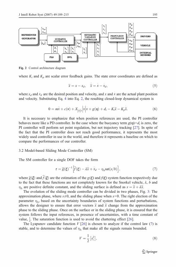
The control and guidance architecture is based on three chained controllers. Eachcontroller’s goal is to generalize the system dynamics for their use by the controllers at ahigher hierarchical level [13], reaching in this way the autonomous following of thetrajectory defined by the navigation system. The closest controller to vehicle hardware isthat of propulsion. It receives thrust input references from the kinematic variablescontroller, of higher hierarchical level, and generates voltage values to be applied to themotors of the thrusters. The kinematic variables controller is in charge of following thekinematic references (surge and yaw velocities) given by the guidance system, and (heaveposition) given by the reference generator of the navigation system. Finally, the highesthierarchical controller is the guidance system, which is dedicated to the carrying out oflocal trajectory tracking in a horizontal plane, taking into account the effect of watercurrents and sideslip [25]. The controller makes null the values of the trajectory followingerrors, de and = e, which are not measured by the integration of angular and linearvelocities, on the contrary, they are estimated from the analysis of the FLS image. In Fig. 2,a diagram of the control architecture, with the nomenclature criteria of Table 1, is shown.

3 Fuzzy Sliding Mode Control Algorithm

In this section the equations and a stability analysis of the resulting close loop of the AFSMcontroller are presented. Additionally, these characteristics are also studied by a simple PIcontroller and a model based SM controller. The controllers have been designed to trackposition and velocity references for the surge, heave and yaw movements.

3.1 Velocity PI Controller (PI)

The basic velocity PI controller for a single-DOF plant takes the form.

t ¼ Kiexþ Kpex� ; ð4Þ

Table 1 Nomenclature

DOF Surge Sway Heave Yaw Pitch Roll

Force/moment tu [N] tw [N] tr [Nm]Velocities x

�u [m/s] x

�v [m/s] x

�w [m/s] x

�p [rad/s] x

�q [rad/s] x

�r [rad/s]

Positions/angles xu [m] xv [m] xw [m] xp [rad] xq [rad] xr [rad]


where Ki and Kp are scalar error feedback gains. The state error coordinates are defined as

ex ¼ x� xd ; ex� ¼ x� � x

�d; ð5Þ

where xd and x�d are the desired position and velocity, and x and x

�are the actual plant position

and velocity. Substituting Eq. 4 into Eq. 2, the resulting closed-loop dynamical system is

0 ¼ mx�� þ c vð Þ þ X x

�j jx� x�� x� þ g ηηð Þ þ di � Kiex� Kpex� : ð6Þ

It is necessary to emphasize that when position references are used, the PI controllerbehaves more like a PD controller. In the case where the buoyancy term g(η)+di is zero, thePI controller will perform set point regulation, but not trajectory tracking [27]. In spite ofthe fact that the PI controller does not reach good performance, it represents the mostwidely used controller in use in the world, and therefore it represents a baseline on which tocompare the performances of our controller.

3.2 Model-based Sliding Mode Controller (SM)

The SM controller for a single DOF takes the form

t ¼ bg ξξð Þ�1 bf ξξð Þ � lex� þ x��d � η$sat s=bð Þ

h i; ð7Þ

where bg xxð Þ and bf xxð Þ are the estimation of the g (ξξ) and f (ξξ) system function respectively dueto the fact that these functions are not completely known for the Snorkel vehicle, l, b andη$ are positive definite constant, and the sliding surface is defined as s ¼ ex� þ lex.

The evolution of the sliding mode controller can be divided in two phases, Fig. 3: Theapproximation phase, where s≠0, and the sliding phase when s=0. The right election of theparameter η$, based on the uncertainty boundaries of system functions and perturbations,allows the designer to ensure that error vectors ex and ex� change from the approximationphase to the sliding phase. Once on the surface or in the sliding phase, it is ensured that thesystem follows the input references, in presence of uncertainties, with a time constant ofvalue, 1

l. The saturation function is used to avoid the chattering effect [26].The Lyapunov candidate function V [26] is chosen to analyze if the control law (7) is

stable, and to determine the values of η$ that make all the signals remain bounded.

V ¼ 1

2s2i� �

; ð8Þ

Fig. 2 Control architecture diagram


If the Lyapunov condition ss� � h sj j is applied, where η is a positive constant, the

derivative will be V� � 0. Thus, from the definition of the sliding surface and expressions

(3) and (7), and for positive values of s all of them bigger than their respective b, this meansthat s

� � h. And solving for η$ yields,

η$ � ηþ bg ξξð Þg ξξð Þ f ξξð Þ � bf ξξð Þ

� �þ x

��d � bg ξξð Þ

g ξξð Þ x��d

� �þ bg ξξð Þ

g ξξð Þ lex� � lex�� þ bg ξξð Þ

g ξξð Þ d ð9Þ

As can be seen in Eq. 9 that the value of η$ depends on the choice of another parameterη, which at the same time is defined by T, or the time that the state vector spends inreaching the sliding condition. The mathematical interpretation of this parameter, forpositive values of s, is T � s0

h .To summarize, all the signals remain bounded, and the velocity error asymptotically

tracks to zero. This approach is an application to underwater vehicles of the generalmethodology reported in [26].

3.3 Adaptive Fuzzy Sliding Mode Controller (AFSM)

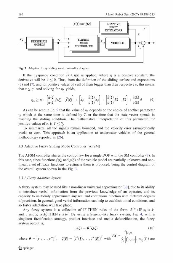
The AFSM controller shares the control law for a single DOF with the SM controller (7). Inthis case, since functions f (ξ) and g(ξ) of the vehicle model are partially unknown and non-linear, a set of fuzzy functions to estimate them is proposed, being the control diagram ofthe overall system shown in the Fig. 3.

3.3.1 Fuzzy Adaptive System

A fuzzy system may be used like a non-linear universal approximator [30], due to its abilityto introduce verbal information from the previous knowledge of an operator, and itscapacity to uniformly approximate any real and continuous function with different degreesof precision. In general, good verbal information can help to establish initial conditions, andso faster adaptation will take place.

Any fuzzy system is a collection of IF-THEN rules of the form: R jð Þ : IF x1 is Aj1

and . . . and xn is Ajn THEN y is B j. By using a Sugeno-like fuzzy system, Fig. 4, with a

singleton fuzzification strategy, product interface and media defuzzification, the fuzzysystem output is,

y ξξξð Þ ¼ q Tζζζ ξξξð Þ ð10Þ

where q ¼ y1; . . . ; ymð ÞT ; ζζζ ξξξð Þ ¼ ζ1 ξξξð Þ; . . . ; ζm ξξξð Þ� �Twith

ζj ξξξð Þ ¼Qni¼1

μAjiξið ÞPm

j¼1

Qni¼1

μAjiξið Þ

� �, μAj

iξið Þ are

Fig. 3 Adaptive fuzzy sliding mode controller diagram


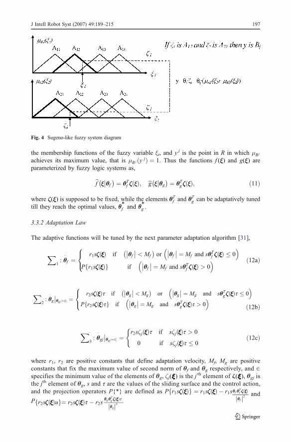
the membership functions of the fuzzy variable ξi, and y j is the point in R in which μB j

achieves its maximum value, that is μB j y jð Þ ¼ 1. Thus the functions f (ξ) and g(ξ) areparameterized by fuzzy logic systems as,

bf ξξ qf�� ¼ qTf ζζζ ξξð Þ; bg ξξ qg

�� ¼ qTg ζζζ ξξð Þ; ð11Þ

where ζ(ξ) is supposed to be fixed, while the elements qTf and qTg can be adaptatively tunedtill they reach the optimal values, θθ*f and θθ*g .

3.3.2 Adaptation Law

The adaptive functions will be tuned by the next parameter adaptation algorithm [31],

X1: q

�f ¼

r1sζζζ ξξξð Þ if qf�� < Mf

� �or qf

�� ¼ Mf and sqTf ζζζ ξξξð Þ � 0

P r1sζζζ ξξξð Þf g if qf�� ¼ Mf and sqTf ζζζ ξξξð Þ > 0

8<: ð12aÞ

X2: q

�g qgj>2�� ¼

r2sζζζ ξξξð Þt if qg�� < Mg

� �or qg

�� ¼ Mg and sqTg ζζζ ξξξð Þt � 0

P r2sζζζ ξξξð Þtf g if qg�� ¼ Mg and sqTg ζζζ ξξξð Þt > 0

8<: ð12bÞ

X3: q

�gj qgj¼2�� ¼

r2sζj ξξξð Þt if sζj ξξξð Þt > 0

0 if sζj ξξξð Þt � 0

(ð12cÞ

where r1, r2 are positive constants that define adaptation velocity, Mf, Mg are positiveconstants that fix the maximum value of second norm of θf and θg respectively, and 2specifies the minimum value of the elements of θg, ζj(ξξξ) is the j

th element of ζ(ξξξ), θgj isthe jth element of θg, s and t are the values of the sliding surface and the control action,and the projection operators P{*} are defined as P r1sζζζ ξξξð Þf g ¼ r1sζζζ ξξξð Þ � r1sθθf θθ

Tf ζζζ ξξξð Þθθfj j2 and

P r2sζζζ ξξξð Þuf g¼ r2sζζζ ξξξð Þt � r2sθθgθθ

Tg ζζζ ξξξð Þtθθgj j2

.

Fig. 4 Sugeno-like fuzzy system diagram


Theorem [34] For a non-linear system (3), consider the controller (7). If the parameteradaptation algorithm (12a, 12b and 12c) is applied, then the system can guarantee that:(a) the parameters are bounded, and (b) closed loop signals are bounded and trackingerror converges asymptotically to zero under the assumption of a fuzzy integrable ap-proximation error.

Proof. Boundedness of θf and θg By considering the adaptation algorithm for θf, theLyapunov candidate function Vf ¼ 1

2θθTf θθf is chosen. If the first line of Eq. 12a is true, then if

|θf |<Mf and V�f ¼ r1s θθ

Tf ζζζζ ξξξð Þ � 0, but if |θf |=Mf then |θf |≤Mf always. If the second line of

Eq. 12a is true, then |θf |=Mf and V�f ¼ r1s θθ T

f ζζζ ξξð Þ � r1sθθfj j2θθTf ζζζ ξξξð Þ

θθfj j2 ¼ 0 that is |θf |≤Mf. To sum up,

θθf tð Þ�� Mf 8t > 0 is guaranteed. In the same way��θθg tð Þ�� Mg 8t > 0 can be proved.

The proof of θg j≥2 may be shown as follows, from Eq. 12c if θg j=2 then θθ�gj Q 0,which implies that θg j≥2 for all elements θg j of θg, and this guarantees that the controller(6) can be constructed.

Proof. Boundedness of s and stability analysis Define the minimum approximation errorw ¼ f

�ξξξ�� bf �ξξξ θθj *f �þ �

g�ξξξ�� bg�ξξξ��θθ*g Þ�t, and assuming that η$ is the parameter to meet the

sliding mode control law (9). From Eqs. 3 and 7 s� ¼ bf �ξξξ��θθ*f �� bf �ξξξ��θθf �þ �bg�ξξξ��θθ*g ��bg�ξξξ��θθg��t þ d þ w� η$sat

�s=b

�,can be shown, in other words,

s� ¼ eθθ T

f ζζζζ ξξξð Þ þeθθ Tg ζζζζ ξξξð Þ þ d þ w� η$sat s=bð Þ; ð13Þ

where eθθf ¼ θθ*f � θθf and eθθg ¼ θθ*g � θθg .Considering the Lyapunov candidate function,

V ¼ 1

2s2 þ 1

r1eθθTf

eθθf þ 1

r2eθθ Tg

eθθg� �; ð14Þ

the derivative of V can easily be shown to be,

V� ¼ ss

� þ 1

r1eθθTf eθθ� f þ 1

r2eθθTg eθθ� g ð15aÞ

V� � swþ I1s

eθθTf θθf θθ

Tf ζζζζ ξξξð Þ

θθf�� T þ I2s

eθθTgþ θθgþθθ T

gþζζζζþ ξξξð Þtθθgþ�� T þ I3eθθT

g2ζζζ2 ξξξð Þs t ð15bÞ

where I1;2;3 ¼0; If the first line of adaptation algorithm is true

1; If the second line of adaptation algorithm is true

(, θg+ denotes the set of θg j>2,

θg2 denotes the set of θgj=2, eθθgþ ¼ θθgþ � θθ*gþ, eθg2 ¼ θθg2 � θθ*g2, ζ+(ξ) and ζ2(ξ) are thebasic function sets corresponding to θg+ and θg2 respectively.

It is necessary to prove that the terms I1, I2 in Eq. 15b are non positives and I3 is nonnegative. For I1= 1 this means |θf |=Mf and s θθTf ζζζζ ξξð Þ > 0, since

��θθf �� ¼ Mf Q��θθ*f �� theneθθTf θθf ¼ �

θθ*f � θθf�Tθθf ¼ 1

2

��θθ*f ��2 � ��θθf ��2 þ ��θθ*f � θθf��2� � 0. Therefore the terms I1 are non

positives. Following the same procedure, the terms I2 can be proved to be non positivestoo. In the case I3=1 and based on Eq. 15b and eθθg2 ¼ θθ*g2� 2> 0, it can be proved that theterms I3 are non negative. Thus, this means V

� � sw. Applying the universal approximationtheorem, it can be expected that the term sw is very small or equal to zero [31]. This impliesV� � 0.


It can be concluded that s, θf and θg are bounded, thus if the reference signal xd isbounded, the system state variable x will be bounded, and that both the velocity trackingerror and the time derivative of the parameter estimates converge asymptotically to zero.However, in the absence of additional arguments, it can not be claimed eitherlimt!1 x tð Þj j ¼ 0, limt!1 s tð Þj j ¼ 0 or that limt!1 eθθf�� ¼ 0 and limt!1 eθθg�� ¼ 0. Thisapproach is the application, for the very first time, to underwater vehicles of the generalmethodology originally reported in [31].

4 Experimental Setup

4.1 The Snorkel Vehicle

The Snorkel vehicle, shown in Fig. 5, is a reduced cost remotely operated UUV. The maingoal of the vehicle is to carry out a scientific and autonomous inspection task in the TintoRiver. The Tinto River is an unknown and remote environment, whose geological andbiological characteristics are causing increased astrobiological interest, due to it being hostto a great variety of extremophile microorganisms with a quimiolitrotophical origin. TheSnorkel vehicle is powered by a 300 W AC power supply. The dry mass of the vehicle is75 kg and its dimensions are 0.7 m long×0.5 m wide and 0.5 m high. The vehicle ispassively stable in the roll and pitch angles. Actuation is provided by four DC electricmotors, two of them are placed in a horizontal plane while the others are in a vertical one.

The electronics architecture of the Snorkel vehicle has been designed ad hoc and isbased on a distributed system. It uses two different communication buses; a deterministicCAN bus inside the vehicle and an Ethernet bus to link the robot with the surface and theteleportation station. The main vehicle CPU is compound by a PC104 board with aPentium-III at 600 MHz and the RT-Linux operative system. It hosts the control algorithmsdescribed in this paper, so a digital version of them with an Euler integration algorithm anda sample period of 100 ms have been used. The rest of the nodes of the bus arecompounded by HCS12 microcontrollers, which are dedicated to a sensors interface andthrusters control. A complete description of this architecture is reported in [25].

Fig. 5 Snorkel robot image


The Snorkel vehicle is tethered, and despite the umbilical cable, can play an importantrole in the dynamics of a small underwater vehicle, there are several reasons that allow as tothink that in this specific application this issue is not going to represent an importantproblem, simplifying the design of the whole system: First, because of the reduced cabledimensions and its neutral buoyancy, with 12 mm of diameter and a length smaller than120 m. This is due to the small lake dimensions, and the ad hoc design of the cable withpower line modem communications with the surface. Second, because there is almost acomplete absence of water currents in the lake, which also reduces the influence of theumbilical cable. And finally, because of the characteristics of the proposed controller, whichadapts the dynamics of the umbilical cable, so that it would be part of the vehicle dynamics.This characteristic can be also seen as an advantage of the proposed controller.

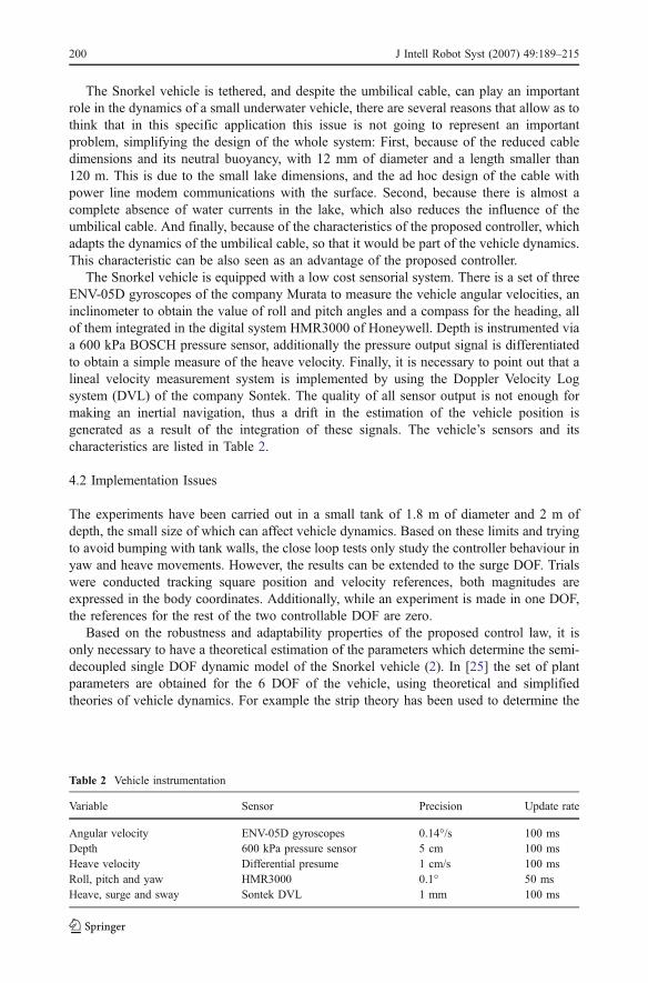
The Snorkel vehicle is equipped with a low cost sensorial system. There is a set of threeENV-05D gyroscopes of the company Murata to measure the vehicle angular velocities, aninclinometer to obtain the value of roll and pitch angles and a compass for the heading, allof them integrated in the digital system HMR3000 of Honeywell. Depth is instrumented viaa 600 kPa BOSCH pressure sensor, additionally the pressure output signal is differentiatedto obtain a simple measure of the heave velocity. Finally, it is necessary to point out that alineal velocity measurement system is implemented by using the Doppler Velocity Logsystem (DVL) of the company Sontek. The quality of all sensor output is not enough formaking an inertial navigation, thus a drift in the estimation of the vehicle position isgenerated as a result of the integration of these signals. The vehicle’s sensors and itscharacteristics are listed in Table 2.

4.2 Implementation Issues

The experiments have been carried out in a small tank of 1.8 m of diameter and 2 m ofdepth, the small size of which can affect vehicle dynamics. Based on these limits and tryingto avoid bumping with tank walls, the close loop tests only study the controller behaviour inyaw and heave movements. However, the results can be extended to the surge DOF. Trialswere conducted tracking square position and velocity references, both magnitudes areexpressed in the body coordinates. Additionally, while an experiment is made in one DOF,the references for the rest of the two controllable DOF are zero.

Based on the robustness and adaptability properties of the proposed control law, it isonly necessary to have a theoretical estimation of the parameters which determine the semi-decoupled single DOF dynamic model of the Snorkel vehicle (2). In [25] the set of plantparameters are obtained for the 6 DOF of the vehicle, using theoretical and simplifiedtheories of vehicle dynamics. For example the strip theory has been used to determine the

Table 2 Vehicle instrumentation

Variable Sensor Precision Update rate

Angular velocity ENV-05D gyroscopes 0.14°/s 100 msDepth 600 kPa pressure sensor 5 cm 100 msHeave velocity Differential presume 1 cm/s 100 msRoll, pitch and yaw HMR3000 0.1° 50 msHeave, surge and sway Sontek DVL 1 mm 100 ms


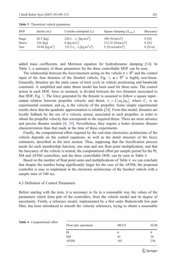
added mass coefficients, and Morrison equation for hydrodynamic damping [14]. InTable 3, a summary of these parameters for the three controllable DOF can be seen.

The relationship between the force/moment acting on the vehicle tt 2 <6 and the controlinput of the four thrusters of the Snorkel vehicle, Fig. 1, u 2 <4 is highly non-linear.Generally, thrusters are the main cause of limit cycle in vehicle positioning and bandwideconstraint. A simplified and static thrust model has been used for these tests. The controlaction in each DOF, force or moment, is divided between the two thrusters associated tothat DOF, Fig. 1. The force generated by the thruster is assumed to follow a square input–output relation between propeller velocity and thrust, t i ¼ Ctwp wp

�� , where Ct is anexperimental constant, and wp is the velocity of the propeller. Some simple experimentalresults show that the quadratic approximation is reliable [24]. From this model, thrusters arelocally fedback by the use of a velocity sensor, associated to each propeller, in order toobtain the propeller velocity that corresponds to the required thrust. There are more advanceand precise thruster models [8, 29]. Nevertheless, they require a better dynamic thrustercharacterization than that made at the time of these experiments.

Finally, the computational effort required by the real-time electronics architecture of thevehicle depends on the control equations, as well as the detail structure of the fuzzyestimators, described in the next section. Thus, supposing that the fuzzification processneeds for each membership function, one sum and one float point multiplication, and thatthe buoyancy of the vehicle is neutral, the computational effort per sample period for the PI,SM and AFSM controllers, and the three controllable DOF, can be seen in Table 4.

Based on the number of float point sums and multiplications of Table 4, we can concludethat despite the number being significantly larger for the case of the AFSM, the proposedcontroller is easy to implement in the electronic architecture of the Snorkel vehicle with asample time of 100 ms.

4.3 Definition of Control Parameters

Before starting with the tests, it is necessary to fix in a reasonable way the values of theparameters which form part of the controllers, from the vehicle model and its degree ofuncertainty. Firstly, a reference model, implemented by a first order Butterworth low pastfilter, has been introduced to smooth the velocity references, trying to obtain a reasonable

Table 3 Theoretical vehicle parameters

DOF Inertia (mi) Coriolis-centripetal (ci) Square damping (X|ui|ui) Buoyancy

Surge 82.5 [kg] 226·x�v � x� r [kg·m/s2] 100 [N/(m/s)2] 0 [N]

Heave 226 [kg] 0 [kg·m/s2] 215.25 [N/(m/s)2] 0 [N]Yaw 10.84 [kg·m2] 133.5·x

�u � x� v[kg·m4/s2] 9 [N·m/(rad/s)2] 0 [N·m]

Float pint operations MULT SUM

PI 6 9SM 45 36AFSM 165 254

Table 4 Computational effort


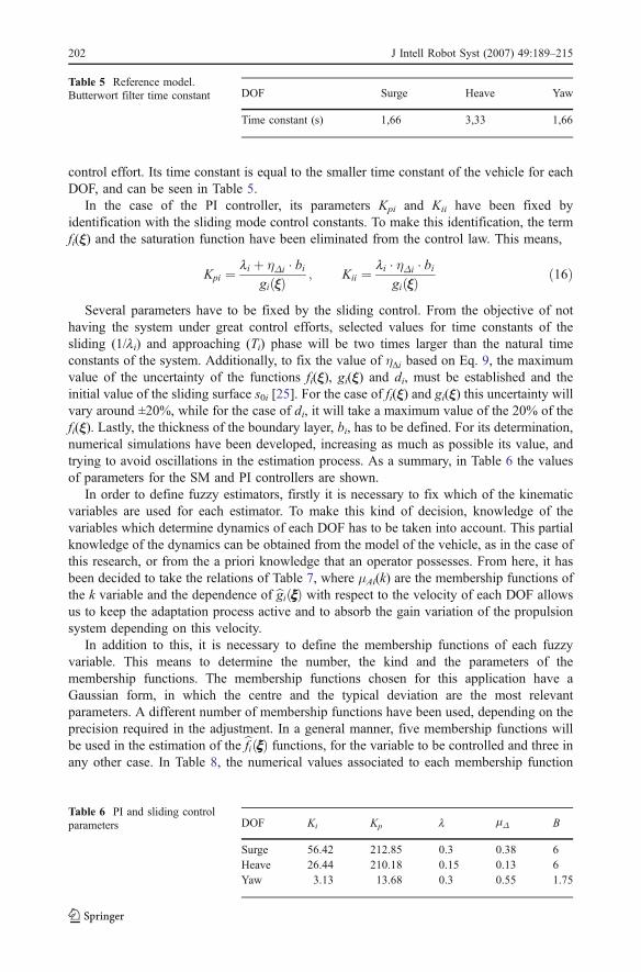
control effort. Its time constant is equal to the smaller time constant of the vehicle for eachDOF, and can be seen in Table 5.

In the case of the PI controller, its parameters Kpi and Kii have been fixed byidentification with the sliding mode control constants. To make this identification, the termfi(ξ) and the saturation function have been eliminated from the control law. This means,

Kpi ¼ li þ ηΔi � bigi ξξð Þ ; Kii ¼ li � ηΔi � bi

gi ξξð Þ ð16Þ

Several parameters have to be fixed by the sliding control. From the objective of nothaving the system under great control efforts, selected values for time constants of thesliding (1/li) and approaching (Ti) phase will be two times larger than the natural timeconstants of the system. Additionally, to fix the value of η$i based on Eq. 9, the maximumvalue of the uncertainty of the functions fi(ξ), gi(ξ) and di, must be established and theinitial value of the sliding surface s0i [25]. For the case of fi(ξ) and gi(ξ) this uncertainty willvary around ±20%, while for the case of di, it will take a maximum value of the 20% of thefi(ξ). Lastly, the thickness of the boundary layer, bi, has to be defined. For its determination,numerical simulations have been developed, increasing as much as possible its value, andtrying to avoid oscillations in the estimation process. As a summary, in Table 6 the valuesof parameters for the SM and PI controllers are shown.

In order to define fuzzy estimators, firstly it is necessary to fix which of the kinematicvariables are used for each estimator. To make this kind of decision, knowledge of thevariables which determine dynamics of each DOF has to be taken into account. This partialknowledge of the dynamics can be obtained from the model of the vehicle, as in the case ofthis research, or from the a priori knowledge that an operator possesses. From here, it hasbeen decided to take the relations of Table 7, where μAi(k) are the membership functions ofthe k variable and the dependence of bgi xxxð Þ with respect to the velocity of each DOF allowsus to keep the adaptation process active and to absorb the gain variation of the propulsionsystem depending on this velocity.

In addition to this, it is necessary to define the membership functions of each fuzzyvariable. This means to determine the number, the kind and the parameters of themembership functions. The membership functions chosen for this application have aGaussian form, in which the centre and the typical deviation are the most relevantparameters. A different number of membership functions have been used, depending on theprecision required in the adjustment. In a general manner, five membership functions willbe used in the estimation of the bfi xxxð Þ functions, for the variable to be controlled and three inany other case. In Table 8, the numerical values associated to each membership function

DOF Surge Heave Yaw

Time constant (s) 1,66 3,33 1,66

Table 5 Reference model.Butterwort filter time constant

DOF Ki Kp l mΔ B

Surge 56.42 212.85 0.3 0.38 6Heave 26.44 210.18 0.15 0.13 6Yaw 3.13 13.68 0.3 0.55 1.75

Table 6 PI and sliding controlparameters


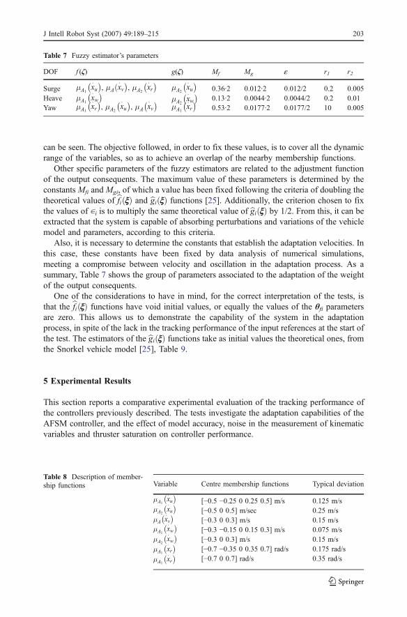
can be seen. The objective followed, in order to fix these values, is to cover all the dynamicrange of the variables, so as to achieve an overlap of the nearby membership functions.

Other specific parameters of the fuzzy estimators are related to the adjustment functionof the output consequents. The maximum value of these parameters is determined by theconstants Mfi and Mgi, of which a value has been fixed following the criteria of doubling thetheoretical values of bfi xxð Þ and bgi xxð Þ functions [25]. Additionally, the criterion chosen to fixthe values of ∈i is to multiply the same theoretical value of bgi xxð Þ by 1/2. From this, it can beextracted that the system is capable of absorbing perturbations and variations of the vehiclemodel and parameters, according to this criteria.

Also, it is necessary to determine the constants that establish the adaptation velocities. Inthis case, these constants have been fixed by data analysis of numerical simulations,meeting a compromise between velocity and oscillation in the adaptation process. As asummary, Table 7 shows the group of parameters associated to the adaptation of the weightof the output consequents.

One of the considerations to have in mind, for the correct interpretation of the tests, isthat the bfi xxð Þ functions have void initial values, or equally the values of the θfi parametersare zero. This allows us to demonstrate the capability of the system in the adaptationprocess, in spite of the lack in the tracking performance of the input references at the start ofthe test. The estimators of the bgi xxð Þ functions take as initial values the theoretical ones, fromthe Snorkel vehicle model [25], Table 9.

5 Experimental Results

This section reports a comparative experimental evaluation of the tracking performance ofthe controllers previously described. The tests investigate the adaptation capabilities of theAFSM controller, and the effect of model accuracy, noise in the measurement of kinematicvariables and thruster saturation on controller performance.

Table 7 Fuzzy estimator’s parameters

DOF f (ζ) g(ζ) Mf Mg e r1 r2

Surge μA1

�x�u

�, μAðx

�v

�, μA2

�x�r

�μA2

�x�u

�0.36·2 0.012·2 0.012/2 0.2 0.005

Heave μA1

�x�w

�μA2

�x�w

�0.13·2 0.0044·2 0.0044/2 0.2 0.01

Yaw μA1

�x�r

�, μA2

�x�u

�, μA

�x�v

�μA1

�x�r

�0.53·2 0.0177·2 0.0177/2 10 0.005

Variable Centre membership functions Typical deviation

μA1

�x�u

�[−0.5 −0.25 0 0.25 0.5] m/s 0.125 m/s

μA2

�x�u

�[−0.5 0 0.5] m/sec 0.25 m/s

μA

�x�v

�[−0.3 0 0.3] m/s 0.15 m/s

μA1

�x�w

�[−0.3 −0.15 0 0.15 0.3] m/s 0.075 m/s

μA2

�x�w

�[−0.3 0 0.3] m/s 0.15 m/s

μA1

�x�r

�[−0.7 −0.35 0 0.35 0.7] rad/s 0.175 rad/s

μA1

�x�r

�[−0.7 0 0.7] rad/s 0.35 rad/s

Table 8 Description of member-ship functions


Table 10 shows the parameters of the body frame references, used to carry out theexperiments. The oscillatory shape permits us to keep the estimation process active. Theseinput references have square and triangular forms, because these types of forms containdifferent spectra components. In this way, the behaviour of the system is analysed forvarious frequencies at the same time versus the use of a sinusoidal signal, avoidingparticular frequency effects and improving the validity of the results.

Some norms to quantitatively compare the performance of each controller have beenadopted. A position error norm for each DOF is calculated as ex ¼ mean xd � xj jð Þ. Thevelocity error norm is calculated as ex� ¼ mean

��x� d � x� ��, and finally the control effort norm of

the corresponding active thruster in each test is calculated as tTOTAL=mean(|td|).

5.1 Comparative Performance with Velocity Reference and Model Adaptation Capabilities

The first section reports a direct comparison of the PI, SM and AFSM controllersperformance, as well as the control effort of each controller, while a yaw velocity referenceis tracked, Table 10. Additionally it attempts to show the performance of the AFSMcontroller to estimate vehicle dynamics, from the fact that a priori vehicle model is purelytheoretical. In order to implement the control law, and based on Snorkel sensorial system, ithas to be emphasized that the real position and position reference are obtain directly byintegrating the real velocity and velocity reference respectively. This will mean a problemof drift in the estimation of the vehicle angular position, but based on vehicle architecture,an angular error is irrelevant, because the guidance controller is in charge of local positiontracking.

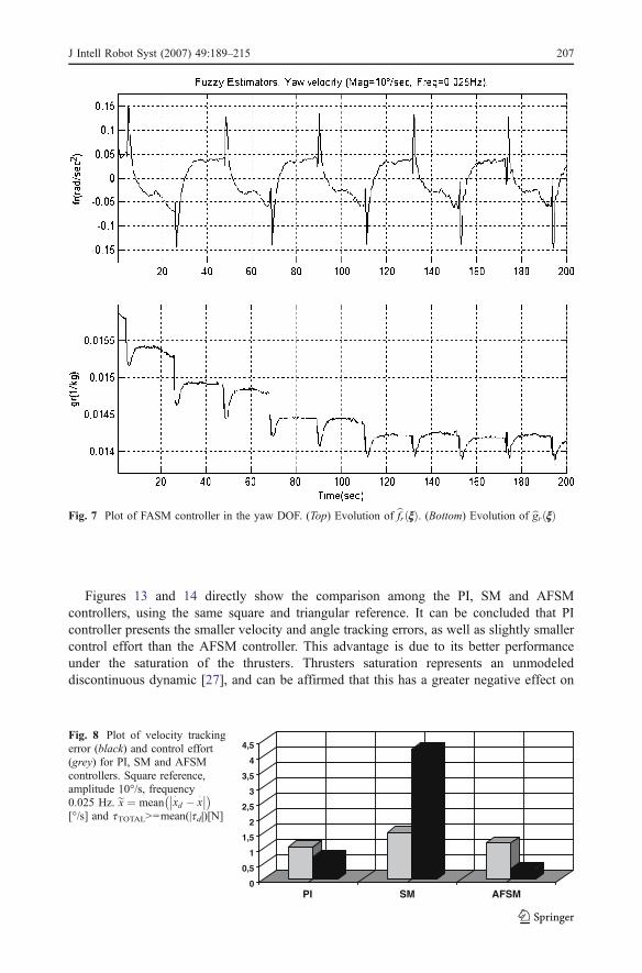
From an analysis of the Fig. 6c we observe that the tracking of the input reference for theAFSM controller is nearly perfect, always with a reasonable control effort, Fig. 6c (bottom),in spite of the oscillatory behaviour when the output value is close to zero. The oscillationcan be caused by an error in the on line algorithm that makes null the offset of thegyroscope signals. The figures correspond to the period after the initial adaptation processof bfr xxxð Þ and bgr xxxð Þ functions, supposing that these have reached their optimal values.

From the beginning of the test, the estimation of the bfr xxxð Þ function, Fig. 7 (top), is stableduring the entire test in spite of the peaks, whose origin is the oscillation of the systemoutput described before. Similarly, the estimation of the bgr xxxð Þ function reaches its stablevalue over the minimum established, Fig. 7(bottom). The appearance of oscillations in these

DOF θθθTf θθθT

g

Surge [0.. 0]45×1 [0.012 0.012 0.012]Heave [0.. 0]5×1 [0.0044 0.0044 0.0044]Yaw [0.. 0]45×1 [0.0177 0.0177 0.0177]

Table 9 Initial values ofθfi and θgi

Reference Amplitude Offset Frequency(Hz)

Period(s)

Yaw velocity 10°/s 0°/s 0.025 40Yaw 50° 70° 0.025 40Depth 0.3 m 0.7 m 0.025 40

Table 10 References


functions attempts to make null the value of the sliding surface in the quickest methodpossible.

Figure 6a and b show the tracking error and the control effort of the PI and SMcontrollers, using the same input reference as in the case of the AFSM controller. It can beeasily observed that the PI controller presents a worse performance and the SM controllereven worse than the AFSM controller. In the case of the SM controller test, the existence oflarge chartering when yaw velocity takes negative values is caused by an error in the

Fig. 6 a Plot of PI controller inthe yaw DOF. (Top) Actual yawvelocity x

�r (- -) and reference

x�rd (–). (Medium) Velocity track-ing error. (Bottom) Thrust of ahorizontal thruster. b Plot of SMcontroller in the yaw DOF. (Top)actual yaw velocity x

�r (- -) and

reference x�rd (–). (Medium) Ve-

locity tracking error. (Bottom)Thrust of a horizontal thruster. cPlot of AFSM controller in theyaw DOF. (Top) actual yaw ve-locity x

�r (- -) and reference x

�rd (–).

(Medium) Velocity tracking error.(Bottom) Thrust of a horizontalthruster


implementation of the control algorithm. In Figs. 8 and 9, this comparison is madeanalytically, using a square and a triangular reference respectively. They conclude thatAFSM controller presents the smaller velocity error, while its control effort is only slightlyhigher than the control effort of the PI controller. This is due to the adaptation capabilitiesof the AFSM controller, based on its fuzzy estimators and the right adaptation law. Theperformance of a model based controller, as the SM controller, depends entirely on theaccuracy of the dynamic plant model used in the designing of the controller. This sectionalso corroborates the lack of accuracy of the theoretical determined dynamical plant modelfor the Snorkel UUV, presented in Section 2.

5.2 Effect of Thruster Saturation with Position Reference

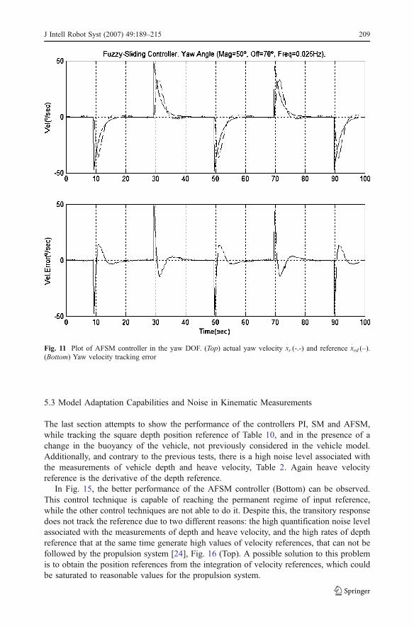
The second set of tests reports a direct comparison of the PI, SM and AFSM controllerperformance, while tracking a position input reference for the yaw angle, Table 10.Nevertheless, this controller will use velocity references as input, as is required by thevehicles architecture. Additionally, it attempts to show the influence of thruster saturation inthe velocity and positions tracking errors. In this test, velocity reference is the derivative ofthe angular reference.

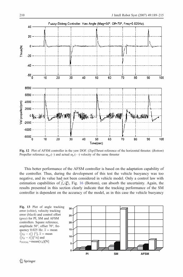
It is evident that there are some deficits in the tracking of the input position and velocityreferences, for the case of the AFSM controller, Figs. 10 and 11. Nevertheless, the finalvalues of the yaw angle and velocities are reached, in spite of the appearance of overshoot.The excessively fast and large velocity reference generates fast and high thrust references,Fig. 12 (top), which cause high turn velocity in the propellers of the horizontal thrusters,Fig. 12 (bottom). The velocity reference of the propellers is achieved by the thrust con-troller, but in spite of that, and by using real data of the propulsion system [23], it can besupposed that the hydrodynamic part of the propulsion system is not as fast as it must be,saturating the thrusters.

Fig. 6 (continued)


Figures 13 and 14 directly show the comparison among the PI, SM and AFSMcontrollers, using the same square and triangular reference. It can be concluded that PIcontroller presents the smaller velocity and angle tracking errors, as well as slightly smallercontrol effort than the AFSM controller. This advantage is due to its better performanceunder the saturation of the thrusters. Thrusters saturation represents an unmodeleddiscontinuous dynamic [27], and can be affirmed that this has a greater negative effect on

Fig. 7 Plot of FASM controller in the yaw DOF. (Top) Evolution of bfr xxð Þ. (Bottom) Evolution of bgr xxð Þ

0

0,5

1

1,5

2

2,5

3

3,5

4

4,5

PI SM AFSM

Fig. 8 Plot of velocity trackingerror (black) and control effort(grey) for PI, SM and AFSMcontrollers. Square reference,amplitude 10°/s, frequency0.025 Hz. ex� ¼ mean

��x� d � x� ��

[°/s] and tTOTAL>=mean(|td|)[N]


the adaptive controllers, because while they are not only based on an inaccurate modelstructure, as the SM controller, the AFSM attempts to estimate the parameter values of thatill-structured plant model. Thus, future work must be done in dealing with handlingadaptation to actuators saturation [22]. Again, the performance of the SM controller isjustified due to the lack of the theoretical model of the Snorkel vehicle.

0

0,5

1

1,5

2

2,5

Pl SM AFSM

Fig. 9 Plot of velocity trackingerror (black) and control effort(grey) for PI, SM and AFSMcontrollers. Triangular reference,amplitude 10°/s, frequency0.025 Hz. ex� ¼ mean

��x� d � x� ��

[°/s] and tTOTAL=meanð|td|Þ[N]

Fig. 10 Plot of AFSM controller in the yaw DOF. (Top) actual yaw angle xr (- -) and reference xrd (–).(Bottom) Yaw angle tracking error


5.3 Model Adaptation Capabilities and Noise in Kinematic Measurements

The last section attempts to show the performance of the controllers PI, SM and AFSM,while tracking the square depth position reference of Table 10, and in the presence of achange in the buoyancy of the vehicle, not previously considered in the vehicle model.Additionally, and contrary to the previous tests, there is a high noise level associated withthe measurements of vehicle depth and heave velocity, Table 2. Again heave velocityreference is the derivative of the depth reference.

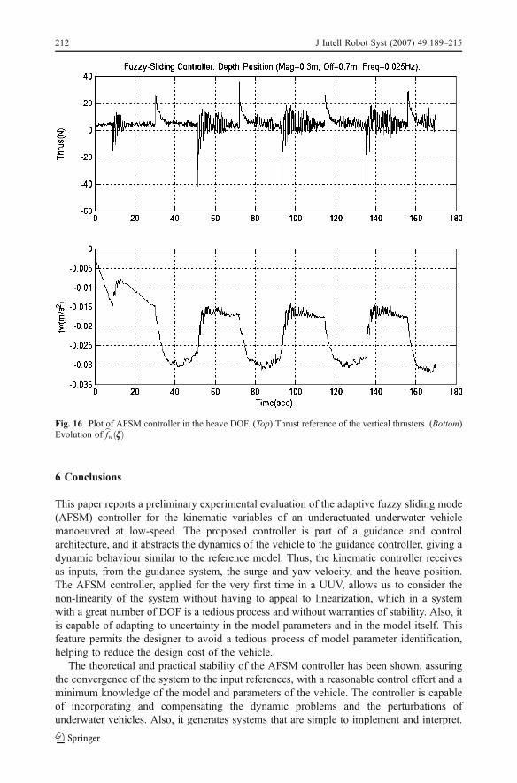
In Fig. 15, the better performance of the AFSM controller (Bottom) can be observed.This control technique is capable of reaching the permanent regime of input reference,while the other control techniques are not able to do it. Despite this, the transitory responsedoes not track the reference due to two different reasons: the high quantification noise levelassociated with the measurements of depth and heave velocity, and the high rates of depthreference that at the same time generate high values of velocity references, that can not befollowed by the propulsion system [24], Fig. 16 (Top). A possible solution to this problemis to obtain the position references from the integration of velocity references, which couldbe saturated to reasonable values for the propulsion system.

Fig. 11 Plot of AFSM controller in the yaw DOF. (Top) actual yaw velocity x�r (-.-) and reference x

�rd (–).

(Bottom) Yaw velocity tracking error


This better performance of the AFSM controller is based on the adaptation capability ofthe controller. Thus, during the development of this test the vehicle buoyancy was toonegative, and its value had not been considered in vehicle model. Only a control law withestimation capabilities of bfw xxð Þ, Fig. 16 (Bottom), can absorb the uncertainty. Again, theresults presented in this section clearly indicate that the tracking performance of the SMcontroller is dependent on the accuracy of the model, as in this case the vehicle buoyancy

Fig. 12 Plot of AFSM controller in the yaw DOF. (Top)Thrust reference of the horizontal thruster. (Bottom)Propeller reference wpd (–) and actual wp (- -) velocity of the same thruster

0

5

10

15

20

25

30

PI SM AFSM

Fig. 13 Plot of angle trackingerror (white), velocity trackingerror (black) and control effort(grey) for PI, SM and AFSMcontrollers. Square reference,amplitude 50°, offset 70°, fre-quency 0.025 Hz. ex ¼ mean��xd � x

�� [°], ex� ¼ mean��x� d � x� ��[°/s] and

tTOTAL=mean(|td|)[N]


was not considered, the SM controller behaves poorly. Thus, we can conclude that a biggereffort must be made in the SM controller design and the vehicle model identification inorder to accomplish a good enough performance with the SM controller.

0

1

2

3

4

5

6

7

PI SM AFSM

Fig. 14 Plot of angle trackingerror (white), velocity trackingerror (black) and control effort(grey) for PI, SM and AFSMcontrollers. Triangular reference,amplitude 50°, offset 70°,frequency 0.025 Hz. ex ¼ mean��xd � x

��[°], ex� ¼ mean��x� d � x� ��[°/s] and

tTOTAL=mean(|td|)[N]

Fig. 15 Plot of actual depth xw (- -) and reference xwd (–) for (Top) PI controller, (Medium) SM controller and(Bottom) AFSM controller. Square reference, amplitude 0.3 m, offset 0.4 m, frequency 0.025 Hz


6 Conclusions

This paper reports a preliminary experimental evaluation of the adaptive fuzzy sliding mode(AFSM) controller for the kinematic variables of an underactuated underwater vehiclemanoeuvred at low-speed. The proposed controller is part of a guidance and controlarchitecture, and it abstracts the dynamics of the vehicle to the guidance controller, giving adynamic behaviour similar to the reference model. Thus, the kinematic controller receivesas inputs, from the guidance system, the surge and yaw velocity, and the heave position.The AFSM controller, applied for the very first time in a UUV, allows us to consider thenon-linearity of the system without having to appeal to linearization, which in a systemwith a great number of DOF is a tedious process and without warranties of stability. Also, itis capable of adapting to uncertainty in the model parameters and in the model itself. Thisfeature permits the designer to avoid a tedious process of model parameter identification,helping to reduce the design cost of the vehicle.

The theoretical and practical stability of the AFSM controller has been shown, assuringthe convergence of the system to the input references, with a reasonable control effort and aminimum knowledge of the model and parameters of the vehicle. The controller is capableof incorporating and compensating the dynamic problems and the perturbations ofunderwater vehicles. Also, it generates systems that are simple to implement and interpret.

Fig. 16 Plot of AFSM controller in the heave DOF. (Top) Thrust reference of the vertical thrusters. (Bottom)Evolution of bfw xxð Þ


From a theoretical point of view, the proposed controller could be defined as acombination of an adaptive and robust system. In this way, it presents the advantages ofrobust control like the capability of adapting to rapid variation of the parameters,perturbations, noise from unmodeled dynamics, and theoretical insensibility to errors of thestate measurements and its derivatives. And also, it presents the advantages of adaptivesystems, like no requirement for prior and precise knowledge of uncertainty, reducing therequired knowledge of system boundaries of uncertainty, and the capacity of improving theoutput performance as the system adapts.

The fuzzy adaptive part of the controller permits us to relax the design conditions of thesliding part, due to perturbations and variation in model parameters which are compensatedand adapted by the fuzzy part of the system. This permits us to decrease the oscillationsdemanded from the propulsion system, which are caused by the high discontinuous gainexisting in pure sliding systems.

One of the restrictions of the fuzzy adaptive part is the low speed of the parametricadjustment, despite the fact that in underwater vehicles this is not usually important. Theadaptation velocity depends on the values of some constants, so that as their values increasethe overshoot also increases. Nevertheless, this lack does not have a special relevance in thesystem due to the fact that it is compensated by the sliding part of the controller.

In order to carry out the tests the simple case semi-decoupled plant model has beenconsidered employing thrust input, constant added mass, constant square drag and constantbuoyancy. We have compared the performance of the proposed controller with the veryused PI controller and a simple model based SM controller. The experiments of the close-loop performance of these systems corroborate the theoretical predictions. Moreover, theexperiments suggest that the AFSM controller is a valid method to be applied in underwatervehicles that outperform the PI and SM controllers using velocity trajectories. Thrustersaturation significantly degrades the performance of AFSM controller, while PI controllershows better performance under this circumstance. The success of a simple model basedSM controller relies on the plant model parameters to be exactly correct, where as AFSM,based on its adaptation capabilities, is not affected by inaccuracy in theoretical plant model.Noise is another factor that significantly affects the performance of the SM controller, andless seriously of the AFSM controller.

In the AFSM controller, the simultaneous estimation of the bf xxð Þ and bg xxð Þ functions, cancause the true values of these functions not to be achieved, but a solution that makes zerothe value of the sliding surface as soon as possible, which is close to the optimal value. Theevolution of both functions is conditioned by the adaptation velocities. The fuzzy estimatorsof the bg xxð Þ functions permit us to absorb the uncertainty associated with the evolution of thegain of the propulsion system, compensating the unmodeled influence that the vehiclevelocities have on the real thrust. Also, they absorb parameter variation such us mass,inertia moments and centre of mass position.

A future work to be developed is to carry out control tests of the kinematic variableswith combined input references, but in order to do that it is necessary to get rid of therestrictions of the water tank. In the same way, tests associated with the guidance controlsystem, considering external perturbations like water currents, will be made. To be able toperform the guidance control, it is necessary to design the navigation algorithms based onthe FLS images that permit us to obtain the values of the trajectory tracking errors.

Acknowledgements We would like to thank certain individuals for their technical assistance in Snorkelrobot building and test preparation: Javier Gomez Elvira, Josefina Torres, Julio Romeral, Javier Martín, JoséAntonio Rodriguez and Patrick C. McGuire. The vehicle has been designed by grants to the Centro deAstrobiología from its sponsoring research organizations, CSIC and INTA.


References

1. Aguilar, L.E., Souères, P., Courdesses, M., Fleury, S.: Robust path following control with exponentialstability for mobile robots. Paper presented at IEEE international conference on robotics and automation,pp. 3279–3284, Leuven, Belgium, 1998

2. Aicardi, M., Casalino, G., Indiveri, G., Aguilar, A., Encarnacao, P., Pascoal, A.: A planar path followingcontroller for underactuated marine vehicles. Paper presented at Mediterranean conference of control andautomation, Dubrovnick, Croatia, 2001

3. Antonelli, G., Chiaverini, S., Sarkar, N., West, M.: Adaptive control of and autonomous underwatervehicle: Experimental results on ODIN. Paper presented at IEEE international symposium incomputational intelligence in robotics and automation, Monterrey, CA, 1999

4. Antonelli, G., Chiaverini, S., Sarkar, N., West, M.: Adaptive control of and autonomous underwatervehicle: experimental results on ODIN. IEEE Trans. Control Syst. Technol. 9, 756–765 (2001)

5. Antonelli, G. (ed.): Underwater Robots. Motion and Force Control of Vehicle-manipulator Systems. In:Springer Tracts in Advanced Robotics, Napoli, Italy (2002)

6. Antonelli, G., Caccavale, F., Chiaverini, S., Fusco, G.: A novel adaptive control law for underwatervehicles. IEEE Trans. Control Syst. Technol. 11(2), 109–120 (2003)

7. Arimoto, S., Miyazaki, F.: Stability and robustness of PID feedback control for robot manipulators ofsensory capabilities. Paper presented at robotics research, first int. symp, Cambridge, MA, 1984

8. Bachmayer, R., Whitcomb, L.: Adaptive parameter identification of an accurate non-linear model formarine thruster. J. Dyn. Syst. Meas. Control 2, 125–131 (2002)

9. Choi, S.K., Yuh, J.: Experimental study on a learning control system with bound estimation forunderwater vehicles. International Journal of Autonomous Robots 3(2/3), 187–194 (1996)

10. Cristi, R., Papoulias, F.A., Healey, A.: Adaptive sliding control mode of autonomous underwatervehicles in the dive plane. IEEE J. Oceanic Eng. 15(3), 462–470 (1991)

11. DeBitetto, P.A.: Fuzzy logic for depth control for unmanned undersea vehicles. Paper presented atsymposium of autonomous underwater vehicle technology, Cambridge, MA, 1994

12. Encarnacao, P.: Non-linear path following control systems for ocean vehicles. Dissertation, UniversidadTécnica de Lisboa, Instituto Superior Técnico, Lisbon (2002)

13. Espinosa, F., López, E., Mateos, R., Mazo, M., García, R.: Application of advanced digital controltechniques to the drive and trajectory tracking systems of a wheelchair for the disabled. Paper presentedat emerging technologies and factory automation, Barcelona, 1999

14. Fossen, T.I. (ed.): Underwater Vehicle Dynamics. Wiley, Chichester (1994)15. Fossen, T.I., Fjellstad, O.E.: Robust adaptive control of underwater vehicles: a comparative study. Paper

presented at IFAC workshop on control applications in marine systems, Trondhein, Norway, 199516. Fossen, T.I., Paulsen, M.: Adaptive feedback linearization applied to steering of ships. Paper presented at

1st IEEE conference on control applications, Dayton, Ohio, 199117. Gee, S.S., Hang, C.C., Zhang, T.: A direct method for robust adaptive non-linear with guaranteed

transient performance. Syst. Control. Lett. 37, 275–284 (1999)18. Goheen, K.G., Jefferys, E.R.: On the adaptive control of remotely operated underwater vehicles. Int. J.

Adapt. Control Signal Process. 4(4), 287–297 (1990)19. Healey, A.J., Lienard, D.: Multivariable sliding mode control for autonomous diving. IEEE J. Oceanic

Eng. 18, 327–339 (1993)20. Hsu, L., Costa, R.R., Lizaralde, F., Cunha da, J.P.V.S.: Dynamic positioning of remotely operated

underwater vehicles. IEEE Robot Autom. Mag. 7, 21–31 (2000)21. Indiveri, G.H., Aicardi, M., Casalino, A.: Non-linear time-invariant feedback control of an underactuated

marine vehicle along a straight course. Paper presented at IFAC conference on manoeuvring and controlof marine craft. Aalborg, Denmark, 2000

22. Johnson, E.N., Calise, A.J.: Pseudo-control hedging: a new method for adaptive control. Paper presentedat workshop on advances in guidance and control technology, Redstone Arsenal, AL, 2000

23. Koivo, H.N.: A multivariable self-tuning controller. Automatica 16(4), 351–366 (1980)24. Manfredi, J.A., Sebastián, E., Gomez-Elvira, J., Martín, J., Torres, J.: Snorkel: Vehículo subacuático para

la exploración del Río Tinto. Paper presented at XXII Jornadas de Automática, Barcelona, 200125. Sebastián, E.: Control y navegación semi-autónoma de un robot subacuático para la inspección de

entornos desconocidos. Dissertation, Universidad de Alcalá, Alcalá de Henares, Madrid (2005)26. Slotine, J.J., Li, W. (eds.): Applied Non-linear Control. Prentice-Hall, Englewood Cliffs, NJ (1991)27. Smallwood, D.A., Whitcomb, L.L.: Model-based dynamic positioning of underwater robotic vehicles:

theory and experiment. IEEE J. Oceanic Eng. 29(1), 169–186 (2004)28. Vaganay, J., Bellingham, J., Leonard, J.: Outlier rejection for autonomous acoustic navigation. Paper

presented at IEEE International conference on Robotics and Automation, Minneapolis, 1996


29. Whitcomb, L., Yoeger, D.: Preliminary experiment in the model-based thrusters control for underwatervehicle positioning. IEEE J. Oceanic Eng. 15(3), (1999)

30. Wang, L.X. (ed.): Adaptive Fuzzy Systems and Control. Prentice-Hall, Englewood Cliff, NJ (1994)31. Wang, J., Get, S.S., Lee, T.H.: Adaptive fuzzy sliding mode control of a class of non-linear systems.

Paper presented at 3rd Asian control conference, Shanghai, 200032. Yoerger, D.R., Slotine, J.J.: Adaptive sliding control of an experimental underwater vehicle. Paper

presented at IEEE international conference on robotics and automation, 199133. Yoerger, D.R., Slotine, J.J.: Robust trajectory control of underwater vehicles. IEEE J. Oceanic Eng. 10

(4), 462–470 (1985)34. Yuh, J.: Learning control for underwater robotics vehicles. IEEE Control Syst. Mag. 14(2), 39–46 (1994)35. Yuh, J.: Design and control of autonomous underwater robots: a survey. Auton. Robots 8, 7–24 (2000)


adaptive fuzzy sliding mode controller for the kinematic ... · adaptive fuzzy sliding mode...

Documents