adaptive finite element methods in...

Adaptive Finite Element Methods in Electrochemistry†

David J. Gavaghan,* Kathryn Gillow, and Endre Su¨li

Oxford UniVersity Computing Laboratory, Wolfson Building, Parks Road, Oxford OX1 3QD, U.K.

ReceiVed April 28, 2006. In Final Form: August 7, 2006

In this article, we review some of our previous work that considers the general problem of numerical simulationof the currents at microelectrodes using an adaptive finite element approach. Microelectrodes typically consist of anelectrode embedded (or recessed) in an insulating material. For all such electrodes, numerical simulation is madedifficult by the presence of a boundary singularity at the electrode edge (where the electrode meets the insulator),manifested by the large increase in the current density at this point, often referred to as the edge effect. Our approachto overcoming this problem has involved the derivation of an a posteriori bound on the error in the numerical approx-imation for the current that can be used to drive an adaptive mesh-generation algorithm, allowing calculation of thequantity of interest (the current) to within aprescribedtolerance. We illustrate the generic applicability of the approachby considering a broad range of steady-state applications of the technique.

1. Introduction

Microelectrodes are widely used for a variety of electroanalysisand electrochemical measurement techniques. Because in generalthere is no direct means of relating the measured quantity (current,potential, etc.) to the underlying chemical system of interest, allsuch techniques are underpinned by mathematical models thatare used to relate these output measurements to the input andchemical parameters of interest (applied potential, concentrations,partial pressures, reaction rates, etc.). The mathematical modelstake the form of reaction-convection-diffusion equations, coupledwith boundary conditions describing the particular electrochemi-cal control technique. Modern microdevices allow the analysisof very fast reactions and extend clinical use to in-vivomeasurements. For these devices, mathematical models areanalytically intractable. As we outline below, numerical solutionis complicated by boundary singularities, the complexity of thechemical processes, and, for clinical devices, by semipermeablemembranes used to prevent surface spoiling (e.g., by proteindeposition). As a result, previous numerical approaches (see ref1 for a comprehensive review) have had difficulty demonstratingaccuracy for general problems.

The long-term goal of our research has therefore been todevelop a general, and preferably completely automated, approachthat will overcome all of these difficulties and generateapproximations for the quantity of interestsin our case, generallythe current flowing in an electrochemical cellsto a user-prescribedtolerance. In this article, we describe our work to date on thedevelopment of adaptive finite element methods (using bothcontinuous and discontinuous approaches, to be described later)for amperometric techniques at a variety of microelectrodegeometries and configurations. All of this work uses the techniqueof deriving an a posteriori error bound to drive the adaptivity,which is somewhat technical and involved from a mathematicalviewpoint. In this review of our work to date, we therefore describein detail only our work on steady-state problems, giving only abrief overview of how we have extended this work to time-dependent problems. Technical mathematical details are givenonly for the simplest model problem in the Appendix, with readers

referred to earlier work for details of the underpinning math-ematics for the more complex examples.

We begin this work with a brief review of previous approachesto the mathematical modeling and numerical simulation ofelectrochemical processes at microelectrodes, together with abrief overview of the use of adaptive numerical techniques inelectrochemistry by other authors.

2. Previous Work

Diffusion processes at microelectrodes are typically modeledin two dimensions by utilizing an inherent symmetry in theelectrode geometry. However, the small size of the electrode(typically in the range of 10-100µm) and the typical time spanof the experiments (the range from the transient out to the steadystate) mean that an account must be taken both of the concentrationgradient normal to the electrode surface (as for a large planarelectrode) and the concentration gradient parallel to the electrodesurface. This parallel component results in a nonuniform currentdistribution over the electrode surface that is usually termed theedge effect, and it is this effect that is usually quoted as makingthe microdisk problem “challenging” (Michael et al.2). In practice,theedgeeffectmeans that thestandard finitedifferenceapproacheson uniform spatial meshes that have been used for 1Delectrochemistry simulation problems since they were introducedby Feldberg in a seminal paper in 19643 have very slow ratesof convergence and thus a prohibitively large number of unknownsis required to compute an accurate solution.

In general, previous approaches that have attempted toovercome these problems fall into five categories:

1. (approximate) analytical solutions;2. special integration technique at the electrode edge to allow

for increased current;3. matching a locally valid series solution near the electrode

edge to the far-field numerical solution;4. conformal maps that either increase the number of points

near the singularity or effectively remove the singularity; and5. mesh refinement to put more points near the singularity.

† Part of the Electrochemistry special issue.* Corresponding author.(1) Alden, J. A. D. Phil. Thesis, University of Oxford, Oxford, U.K., 1998.

(2) Michael, A. C.; Wightman, R. M.; Amatore, C. A.J. Electroanal. Chem.1989, 267, 33.

(3) Feldberg, S. W.Anal. Chem.1964, 36, 505.

10666 Langmuir2006,22, 10666-10682

10.1021/la061158l CCC: $33.50 © 2006 American Chemical SocietyPublished on Web 09/27/2006

2.1. Approximate Analytical Solutions.The only problemfor which a known simple closed-form analytical solution existsis that of steady-state diffusion to a microdisk electrode. Thiswas first presented by Saito in 19684 and further simplified byCrank and Furzeland in 1977.5 As a result, it has become a verycommon test problem for numerical methods. However, ap-proximate analytical solutions have been developed for a varietyof other problems including chronoamperometry at microband6-9

and microdisc10-13 electrodes, linear sweep voltammetry atmicroband14 and microdisc15 electrodes, steady-state E, ECE,and DISP1 reactions at channel microband electrodes,16-20 andEC′ reactions at inlaid and recessed microdisk electrodes.21,22

Although these solutions may not be exact, the authors are oftenable to give an indication of their relative accuracy, so thesesolutions are very useful for comparison with numericalsimulations. More recently, Mahon and Oldham23 revisited theproblem of finding the transient current at the disk electrodeunder diffusion control and derived two overlapping short- andlong-time polynomial functions that are shown to give excellentagreement with all previous work.

2.2. Allowing for Increased Current. This approach wasdeveloped by Heinze for chronoamperometry24 and cyclicvoltammetry25 at microdisk electrodes. It uses a special methodof flux integration at the edge of the electrode. However, thismethod appears to be very problem-dependent, and thus itseems unlikely that it could provide the basis for a generalsimulation algorithm. In addition, no attempt is made to correctthe effect that the boundary singularity has on the concentrationvalues.

2.3. Local Series Solutions.This approach was first used byCrank and Furzeland5 for steady-state diffusion to a microdiskelectrode and was subsequently adopted by Gavaghan andRollett26 for the corresponding time-dependent problem andfurther developed for use with the finite element method byGalceran et al.27 The idea is to find a series solution that is validin the neighborhood of the singularity and to use a finite differencescheme further away. By comparing the number of nodes required

to achieve a given accuracy in the current, it is clear that usingthe series solution is much more efficient than a standard finitedifference method on a regular mesh.

2.4. Conformal Mapping Techniques.The first type of map,as proposed by Taylor et al.,28 is designed to increase the densityof points in the neighborhood of the singularity. Essentially themap leads to a mesh that expands in both spatial directions.However, as Taylor et al. note, a poorly chosen grid expansionfactor may be counterproductive and lead to large errors. Inaddition, it is not obvious how to choose the factors.

The second type, as used by Michael et al.,2 Verbrugge andBaker,29and Amatore and Fosset,30essentially “folds” the radialaxis at the electrode edge, which effectively removes thesingularity. All of the maps lead to a problem in the transformedcoordinates that are solved using finite difference schemes ona regular mesh.

The map used by Michael et al. is essentially a transformationto oblate spherical coordinates, and this was used successfullyto study cyclic voltammetry at microdisk electrodes. They alsoshowed that the map could be used for the simulation of coupledchemical steps by applying it to an EC′ mechanism. This mapwas also used by Deakin et al.31 for cyclic voltammetry atmicroband electrodes and by Lavagnini et al.32for the simulationof voltammetric curves at microdisk electrodes.

Verbrugge and Baker29 extended this work. They used atransformation that maps the infinite strip produced in ref 2 intoa rectangle. They then used these new coordinates to studychronoamperometry at a microdisk electrode.

The conformal map proposed by Amatore and Fosset30 hasthe advantage of producing a finite rectangle in the transformedspace. This was used to study steady-state and near-steady-statediffusion at microdisk electrodes. The advantage of thesetransformations to a finite domain is that the far-field boundaryconditions may be applied exactly. This cannot be done in aninfinite domain. Instead the far-field conditions have to be appliedat a sufficient distance from the electrode surface in the hope thatthe truncated problem will accurately approximate the trueproblem.

Alden and Compton34 also use the map described in ref 30 togenerate working curves for ECE, DISP1, EC2E, DISP2, andEC′ mechanisms at microdisk and spherical/hemisphericalelectrodes. In addition, they have compared this map to the onein ref 29, and they claim that it is superior in that it is moreefficient for diffusion-only processes and the matrices resultingfrom a finite difference discretization are better conditioned.

More recently, Oleinick, working with Amatore and Svir,33

used a quasi-conformal mapping technique to derive what areclaimed to be the most accurate and efficient simulations to datefor diffusion at microdisk electrodes. These authors also comparetheir approach to that of Amatore and Fosset.

The main drawback to the conformal map approach is that theequations in the transformed coordinates are far more complexthan those in the original coordinates and deriving the transformedpartial differential equation may be very complicated (and mustbe done afresh for each new system of equations that is tackled).In addition, as observed by Taylor et al.,28 poorly chosen

(4) Saito, Y.ReV. Polarogr. (Jpn.)1968, 15, 177.(5) Crank, J.; Furzeland, R. M.J. Inst. Math. Its Appl.1977, 20, 355.(6) Aoki, K.; Tokuda, K.; Matsuda, H.J. Electroanal. Chem.1987, 230,

61-67.(7) Aoki, K.; Tokuda, K.; Matsuda, H.J. Electroanal. Chem.1987, 225,

19-32.(8) Oldham, K. B.J. Electroanal. Chem.1981, 122, 1-17.(9) Szabo, A.; Cope, D. K.; Tallman, D. E.; Kovach, P. M.; Wightman, M.

J. Electroanal. Chem.1987, 217, 417-423.(10) Aoki, K.; Osteryoung, J.J. Electroanal. Chem.1981, 122, 19.(11) Aoki, K.; Osteryoung, J.J. Electroanal. Chem.1984, 160, 335.(12) Rajendran, L.; Sangaranarayanan, M. V.J. Electroanal. Chem.1995,

392, 75-78.(13) Shoup, D.; Szabo, A.J. Electroanal. Chem.1982, 140, 237.(14) Aoki, K.; Tokuda, K.J. Electroanal. Chem.1987, 237, 163-170.(15) Aoki, K.; Akimoto, K.; Tokuda, K.; Matsuda, H.; Osteryoung, J.J.

Electroanal. Chem.1984, 171, 219.(16) Ackerberg, R. C.; Patel, R. D.; Gupta, S. K.J. Fluid Mech.1977, 86,

49.(17) Aoki, K.; Tokuda, K.; Matsuda, H.J. Electroanal. Chem.1987, 217,

33.(18) Leslie, W. M.; Alden, J. A.; Compton, R. G.; Silk, T.J. Phys. Chem.

B 1996, 100, 14130.(19) Levich, V. G.Physiochemical Hydrodynamics; Prentice-Hall: Englewood

Cliffs, NJ, 1962.(20) Newman, J.Electroanal. Chem.1973, 6, 187.(21) Galceran, J.; Taylor, S. L.; Bartlett, P. N.J. Electroanal. Chem.1999,

466, 15.(22) Galceran, J.; Taylor, S. L.; Bartlett, P. N.J. Electroanal. Chem.1999,

476, 132.(23) Mahon, P. J.; Oldham, K. B.Electrochim. Acta2004, 49, 5041.(24) Heinze, J.J. Electroanal. Chem.1981, 124, 73.(25) Heinze, J.Ber. Bunsen-Ges. Phys. Chem.1981, 85, 1096.(26) Gavaghan, D. J.; Rollett, J. S.J. Electroanal. Chem.1990, 295, 1.(27) Galceran, J.; Gavaghan, D. J.; Rollett, J. S.J. Electroanal. Chem.1995,

394, 17.

(28) Taylor, G.; Girault, H. H.; McAleer, J.J. Electroanal. Chem.1990, 293,19.

(29) Verbrugge, M. W.; Baker, D. R.J. Phys. Chem. B1992, 96, 4572.(30) Amatore, C. A.; Fosset, B.J. Electroanal. Chem.1992, 328, 21.(31) Deakin, M. R.; Wightman, R. M.; Amatore, C. A.J. Electroanal. Chem.

1986, 215, 49-61.(32) Lavagnini, I.; Pastore, P.; Magno, F.; Amatore, C. A.J. Electroanal.

Chem.1991, 316, 37.(33) Oleinick, A.; Amatore, C.; Svir, I.Electrochem. Commun.2004, 6, 588.(34) Alden, J. A.; Compton, R. G.J. Phys. Chem. B1997, 101, 9606.

AdaptiVe Finite Element Methods in Electrochemistry Langmuir, Vol. 22, No. 25, 200610667

conformal maps may be counterproductive, and different mapsmay perform well for different problems, making the choice ofconformal map difficult. In addition, there is no control over theerror in the subsequent simulations, and it is gaining such controlthat leads to the adaptive mesh refinement approach that is theprimary focus of this article.

2.5. Mesh Refinement.As we will show below, these problemscan be overcome by using a mesh refinement approach withinthe numerical method. This approach is standard for the numericalsimulation of 1D problems in electrochemistry, with Feldberg(with various co-workers) again having introduced the keyconcepts into the electrochemical literature.35-37 This approachwas used in two dimensions by Gavaghan38-40 for steady-statediffusion, chronoamperometry, and linear sweep voltammetryat microdisk electrodes and by Bartlett and Taylor41 for recessedmicrodisk electrodes. The idea is to use a finer mesh where theerror is large, for example, at the boundary singularity at theelectrode edge for inlaid disks and along the electrode surfaceand at the corner singularity for recessed disks. The mesh thenexpands until it is very coarse at large distances from these points.

Alden and Compton have also used expanding meshes forstudying reactions at channel microband electrodes. These authorsuse uniform meshes parallel to the electrode surface butexponentially expanding meshes perpendicular to it. However,this still required over one million mesh points for an accurateapproximation of the current. Even more mesh points were neededfor low flow rates; indeed for very low flow rates these simulationsdid not provide accurate approximations of the current becauseof the excessive memory requirements.

That these methods can give very accurate solutions for boththe microdisk and microband has been confirmed in two excellentrecent review papers by Britz and co-workers.42,43These paperscompare the results from the three primary approaches (analytic,conformal map, and mesh refinement) to give a set of referencevalues for each of these problems that are accurate to better than0.1% at all times in both cases. These papers provide an excellentoverview and reference to all previous work on these problems.

However, the drawback with all of these early attempts atusing mesh refinement is that the refinement strategy is entirelyheuristic and often relies upon knowledge of the analytic solutionor an accurate analytic approximation to assess the accuracy andconvergence of the numerical method. This is also costly giventhe slow convergence. In either case, there is no reliable gaugeof how accurate the solution is on a given (refined) mesh norof whether the mesh is in any way optimal. Clearly, this is arather ad hoc approach and requires the inefficient interventionof the user.

Our aim when we began the work reviewed in this article wastherefore to produce accurate and efficient algorithms toapproximate the current using the finite element method. Thishas allowed us throughout our subsequent work to build a rigorousmathematical analysis that can be used to generate meshes uponwhich we can approximate the quantity of interest, in our case,the current, to within a prescribed tolerance, eliminating theneed for excessive convergence testing or the ad hoc meshgeneration approach described above.

Other authors have considered using an adaptive finite elementmethod approach in electrochemistry. Perhaps the most com-prehensive body of work has been conducted by Bieniasz usinga patch-adaptive approach. (See a series of papers beginningwith ref 44 to the most recent, ref 45.) This work covers a hugerange of electrochemical application problems but to date isrestricted to one spatial dimension. In two spatial dimensions,Nann and Heinze46,47 used a gradient-based approach to drivethe adaptivity, but this again requires a heuristic approach todetermining when convergence has been achieved. Abercrombieand Denuault48 built upon our early work to consider alternativeelectrode geometries and also introduced a patch recoverytechnique that has the potential to improve convergence ratesand accuracy in some instances.

3. Example Problems Considered

In this article, we will consider the generic applicability of ourapproach by solving four model problems that each illustrate itsability to overcome a particular numerical difficulty encounteredby previous authors. First, the simplest possible problem of findingthe steady-state current to a microdisk electrode (and for whichwe have a closed-form analytical solution) allows us to give acomprehensive description of the mathematics behind theapproach (although the technical details are left for the Appendix)and to illustrate how the adaptive algorithm automaticallygenerates meshes that provide increasingly accurate solutions tothe problem. The problem of a steady-state solution of a first-order EC′ reaction (catalytic reaction mechanism) at a recessedmicrodisk has been chosen because by varying the governingreaction rate the reaction layer can be confined within the recessor can spread beyond the recess and be affected by the numericalproblems arising from the corner singularity at the mouth of therecess. The third problem considered, that of the steady-statecurrent at a channel microband electrode, allows us to illustratethe use of the method in Cartesian (rather than cylindrical)coordinates and to extend the treatment to a range of more complexreaction mechanisms.

These three problems are each treated using thecontinuousGalerkin finite element method, but as we show for the thirdproblem (the channel microband electrode), the more recentlydevelopeddiscontinuousGalerkin finite element method (DG-FEM) has strong advantages for certain problems (in this case,avoiding the need to stabilize the numerical approach inconvection-dominated problems). The advantages of the DGFEMapproach become even more apparent in the fourth model problemthat we considerscalculating the steady-state current at amembrane-covered Clarke electrode.

We end this article by presenting some previously unpublishedwork that illustrates how it is possible to utilize the fact that incalculating the a posteriori error bound we must calculate a higher-order solution to the dual problem. This allows us to derive analternative formulation for the current in terms of this higher-order solution, providing large improvements to the accuracy ofthe current calculation at no extra cost. Finally, we give a briefoverview of how we have extended this work to time-dependentproblems.

(35) Feldberg, Stephen W.J. Electroanal. Chem.1981, 127, 1.(36) Feldberg, Stephen W.; Goldstein, Charles I.J. Electroanal. Chem.1995,

397, 1.(37) Mocak, J.; Feldberg, S. W.J. Electroanal. Chem.1994, 378, 31.(38) Gavaghan, D. J.J. Electroanal. Chem.1998, 456, 1-12.(39) Gavaghan, D. J.J. Electroanal. Chem.1998, 456, 13-23.(40) Gavaghan, D. J.J. Electroanal. Chem.1998, 456, 25-35.(41) Bartlett, P. N.; Taylor, S. L.J. Electroanal. Chem.1998, 453, 49.(42) Britz, D.; Poulsen, K.; Strutwolf, J.Electrochim. Acta2004, 50, 107.(43) Britz, D.; Poulsen, K.; Strutwolf, J.Electrochim. Acta2005, 51, 333.

(44) Bieniasz, L. K.J. Electroanal. Chem.2000, 481, 115.(45) Bieniasz, L. K.J. Electroanal. Chem.2004, 565, 273.(46) Nann, T.; Heinze, J.Electrochem. Commun.1999, 1, 289.(47) Nann, T.; Heinze, J.Electrochim. Acta2003, 48, 3975-3980.(48) Abercrombie, S. C. B.; Denuault, G.Electrochem. Commun.2003, 5,

647-656.(49) Østerby, O. Technical Report DAIMI PB-534, Department of Computer

Science, University of Aarhus, Ny Munkegade, Bldg. 540, DK-8000 Aarhus C,Denmark, 1998.

10668 Langmuir, Vol. 22, No. 25, 2006 GaVaghan et al.

4. Simplest Model Problem

We begin our review with the first problem that we consideredand the one that is probably the simplest possible problem of thistypesdetermining the steady-state current at a microdisk elec-trode. Because this problem has a closed-form analytic solution,4

it makes an ideal model problem, and we give a full descriptionof our approach here, including the technical derivations of thenecessary a posteriori bounds83 in the Appendix.

We consider the simple reaction mechanism

at a disk electrode. By assuming semi-infinite mass transportand utilizing the axial symmetry of the problem, the governingsteady-state diffusion equation can be written in cylindrical polarcoordinates as

with u ) c/c0, wherec0 is the bulk concentration of speciesA.Here, the spatial coordinates have been normalized with respectto the electrode radiusa.

4.1. Boundary Conditions.Assuming fast enough kinetics toensure zero concentration on the electrode surface, the boundaryconditions are

The boundary conditions onz ) 0 ensure that there is aboundary singularity at (1, 0) where∂u/∂r is discontinuous,causing problems for standard numerical techniques.

We also note that currently we are required to solve the problemon a semi-infinite domain (0,∞) × (0, ∞). However, to solvethe problem numerically we must use a finite region [0,rmax] ×[0, zmax]. Because the analytical solution for the concentrationfield is known for this problem (see below), we may test ournumerical algorithm by choosing any values forrmax andzmax

and using the exact solution as the boundary condition on theseparts of the boundary. Most of our numerical results are producedusing this approach. Alternatively, we could choose large valuesof rmax andzmax and apply the boundary conditionu ) 1, andwe shall also present results using this approach.

4.2. Current. The quantity of interest in this problem is thenondimensional current at the electrode surface given by

whereI′ is the dimensional current.4.3. Exact Solution.An exact solution to this problem was

given by Saito4 in 1968

with J0 being the zeroth-order Bessel function. Differentiatingthis and substituting into eq 4 gives the familiar value for thenondimensional current ofI ) 1.

Crank and Furzeland5 gave an alternative form of this solutionas

which is more convenient when comparing to numericalapproximations. We also use this form of the solution as theboundary condition onr ) rmax andz ) zmax.

4.4. Numerical Techniques.Our numerical technique is basedon the finite element method (FEM) and is described in detailin the Appendix. Use of the FEM involves obtaining the numericalsolution of the governing partial differential equations bysubdividing the domain into triangles and obtaining piecewiselinear approximations to that solution on each triangle. Ourprimary interest is in calculating an estimate of the current, whichwe will denote byIest, to within a user-specified tolerance, so werequire methods of estimating the error in the numericalapproximation. If the exact value of the current is denoted byI, then the usual standard theoretical bounds on the error|I -Iest| can be derived without the need to findIest first. These areknown as a priori error bounds and indicate the expected orderof convergence of the solution. Unfortunately, these bounds areusually of the form|I - Iest| e Chk, whereh is the mesh size(or the largest mesh size on a nonuniform mesh),C is someconstant that is dependent on the exact solution of the partialdifferential equation, andk depends on both the degree of theapproximating polynomial and the regularity of the true solutionu to the PDE. Such bounds are useful in that they show the rateat which the method converges ash f 0; however, in generalthe size of the constantC is not known, and hence the bound isnot computable. All of our work therefore makes use of a posteriorierror bounds, which are much more useful because they can beexpressed in terms of the finite element solutionuh in such a waythat they are computable and can therefore be used as the basisof an adaptive mesh refinement strategy. As we show below, thisthen ensures that the quantity of interest (here, the current) isboth reliably and efficiently computed.

The details of how such an a posteriori bound is calculatedis rather technical and involved and is therefore given only inthe Appendix. There we also outline how this bound can beincorporated into an adaptive finite element algorithm that ensuresthe calculation of the current to within a user-defined errortolerance with near-optimal levels of computational effort.

4.5. Results.Using the adaptive algorithm described in theAppendix, a series of computational meshes is derived uponwhich we must calculate the solution and the a posteriori errorbound. The algorithm terminates when the error bound is lessthan TOL, a user-defined tolerance, and at this point, the numericalestimate of the current has an error of at most TOL. In thisexample, we choose a value of TOL) 0.05; that is, we requestat most a 5% error in the current. As we show (and as might beexpected), in practice we obtain greater accuracy than this becausethe a posteriori error bound overestimates the error (in this case,by a factor of about 3.)

Takingrmax) zmax) 2 to define the solution region (and usingeq 6 to define the solution onrmaxandzmax), we choose to beginwith a regular mesh with 32 triangles. (Note that we are utilizingaxial symmetry to render the problem in 2D cylindricalcoordinates and that this cylindricity is built into the governingequation, eq 2.) In Table 1, we show the number of triangles(n_tri), the number of nodes (n_nods), currents, and error estimateson the resulting sequence of meshes that is generated by our

A ( ne- ) B (1)

∂2u

∂r2+ 1

r∂u∂r

+ ∂2u

∂z2) 0 (2)

u ) 0 r e 1 z ) 0

∂u∂n

) 0 r > 1 z ) 0

r ) 0 z g 0 (3)

u ) 1 r, z f ∞

I ) π2∫0

1(∂u∂z)z)0

r dr ) I′4FDc0a

(4)

u(r, z) ) 1 - 2π∫0

∞sinmm

J0(rm)e-zmdm (5)

u )

1 - 2π

sin-1 2

xz2 + (1 + r)2 + xz2 + (1 - r)2 z > 0

0 0 e r e 1, z ) 0

1 - 2π

sin-11r r > 1, z ) 0

(6)


adaptive algorithm. The effectivity index is the estimated errordivided by the actual error and gives a measure of the “sharpness”of the error bound. (Clearly, an ideal algorithm will result in anindex value of 1, although in practice it will always be greaterthan 1.) It is only because we know the exact value of the currentin this case that the effectivity index is computable.

The results of this process allow us to calculate the currentto our specified accuracy on a remarkably coarse mesh; the sixthand final mesh in Table 1 actually gives a value of the currentthat is accurate to almost 1% using only 391 unknowns andminimal CPU time.

The meshes generated by the algorithm are given in Figure1. It is immediately clear that our algorithm is able to determinevery quickly (by the third mesh) that the numerical errors arecaused by the boundary singularity, and successive meshes homein on this area, successively reducing the level of error in theoverall calculation of the current until the required tolerance isattained.

4.5.1. Comparison with Regular Meshes.Just how much betterthis approach is can be illustrated by comparing the adaptiveapproach to the use of a simple regular mesh constructed bydividing the domain intoN equal spacings in each coordinatedirection and triangulating by joining the top left corner of eachsquare to the bottom right. We can also use this comparison toshow the superiority of the approximationNψ(uh) (cf. eq 55 inthe Appendix) for the current.

We use a regular mesh and approximate the current usingNψ(uh): as can be seen, halving the mesh spacing roughly halvesthe error in the current (Table 2), suggesting that the error in thecurrent is orderO(h). This is backed up by the a priori errorbound derived in ref 51. A similar level of accuracy to that ofthe adaptive algorithm (an error of around 1%) requires around100 mesh spacings in each direction, a total of 10 201 nodesaltogether, and over 30 times the CPU time.

The standard method of calculating the current used inelectrochemistry is simply to insert the numerical solutionuh

into the original definition of the current; that is, the current isgiven by

instead of eq 55. In Table 3, we show that this approximationconverges to the true value,Nψ(u), at less than half the rate ofNψ(uh); estimating the error between eq 7 and the exact valueof the current to beO(h0.4) means that we would require over1.5× 1013 nodes using eq 7 to achieve the same accuracy as thesixth adaptive mesh gave with only 391 nodes using eq 55. Itis therefore very clear that it is better to estimate the currentusing the expressionNψ(uh) defined by eq 55.

4.5.2. Results for Large rmaxand zmax. Finally, we present theresults obtained from the adaptive algorithm by choosingrmax

) zmax) 80 and applying the boundary conditionu ) 1 on theseparts of the boundary. In Table 4, we show the details of theresulting sequence of meshes that is generated by our adaptivealgorithm. Again we see that relatively few nodes are needed toestimate the current accurately. The erratic values of the effectivityindex on the finer meshes are due to the fact that the exact solutionof the problem we are solving is slightly larger than unity (becausewe are applying a boundary condition that is slightly larger thanit should be).

The part of the final mesh closest to the electrode surface isshown in Figure 2 and has the same characteristics as the previousmeshes.

5. Recessed Disk Electrode

The power of the adaptive finite element technique describedabove is particularly clear when we consider our second modelproblem of the recessed disk electrode. We consider the EC′reaction mechanism (catalytic reaction mechanism) for whichwe have a means of obtaining an analytic solution and are ableto show that our method can give good accuracy on relativelycoarse meshes because it picks out those features of the problemthat cause numerical difficulties and refines the mesh only inthose areas.

5.1. Theory.We consider the case ofSbeing present in a largeexcess so that we can assume pseudo-first-order kinetics,22,52,53

allowing the EC′ mechanism to be described by

wherek is the pseudo-first-order reaction rate,n is the numberof electrons involved, andS andY are electroinactive species.Here we have assumed that the equilibrium constant for thereaction is so large that the reverse process can be ignored. Thegeometry of the problem is shown in Figure 3.

Following refs 22 and 53, a nondimensional concentrationucan be defined as

where cB is the concentration of species B andcBs is the

concentration of B on the electrode surface. Normalizing thespatial coordinates with respect to the electrode radius allowsthe radius to be taken to be equal to 1 in all simulations. Theconcentration,u, then satisfies

with

being the dimensionless reaction rate anda being the actualelectrode radius.DB is the diffusion coefficient of B. The boundaryconditions of the problem are then

with the normalized current given by

The numerical results that we obtain will be compared to theexact solution and approximate analytical solutions of Galceran

(50) Gavaghan, D. J.J. Electroanal. Chem.1997, 420, 147.(51) Harriman, K.; Gavaghan, D. J.; Houston, P.; Su¨li, E. Electrochem.

Commun.2000, 2, 157.

π2∫0

1(∂uh

∂z)z)0

r dr (7)

A ( ne- f B (8)

B + S98k

A + Y

u )cB

cBs

(9)

-∇2u + Ku ) 0 (10)

K ) ka2

DB(11)

u ) 1 r e 1 z ) 0

u f 0 r, z f ∞∂u∂n

) 0 r ) 0 z > 0 (12)

r ) 1 0 e z e L

r > 1 z ) L

I ) - π2∫0

1(∂u∂z)z)0

r dr (13)


et al.,22 which hold assuming that pseudo-first-order conditionsare maintained.

5.2. Results.To illustrate the power of the method in pickingout the salient features of the problem, we consider only the case

(52) Denuault, G.; Fleischmann, M.; Pletcher, D.; Tutty, O. R.J. Electroanal.Chem.1990, 280, 243.

(53) Rajendran, L.; Sangaranarayanan, M. V.J. Phys. Chem. B1999, 103,1518.

Figure 1. Meshes produced by an adaptive finite element method for the steady-state disk electrode problem.


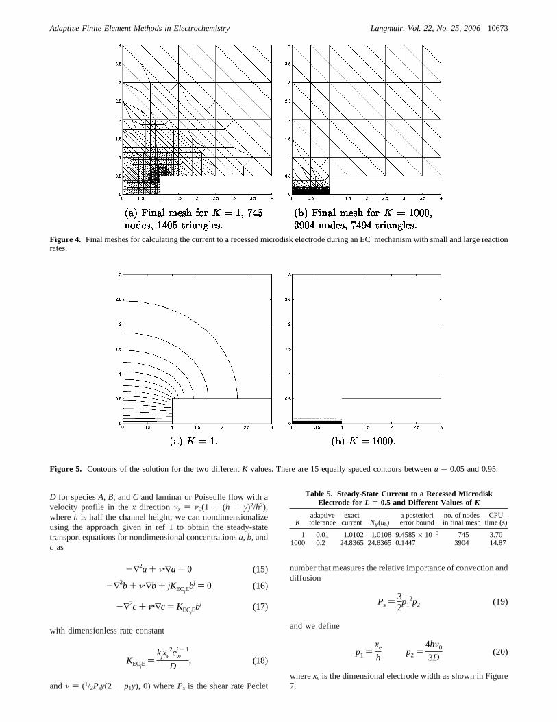
of L ) 0.5 and compare with the analytical results forK ) 1 and1000. The adaptive tolerance for each case is chosen to guarantee1% accuracy in the estimated current. The final mesh for eachof the problems is shown in Figure 4, and these look as we wouldexpect. For the lowerK value, diffusion dominates, and the cornersingularity causes a problem when evaluating the current;consequently, more nodes are needed near the corner. For thehigherK value, the reaction takes place almost entirely withinthe recess, so the mesh may remain coarse further away. In fact,we see that the mesh size above the electrode surface isproportional to the thickness of the reaction layer, which is knownto be K-1/2. These ideas are shown more clearly in Figure 5,which depicts the contours of the solution for each value ofK.It is clear that our completely automated mesh generationalgorithm is able to pick out the features in the solution that willhave an impact on the simulated current as the governingparameters (in this case,K andL) are varied and will refine themesh appropriately. The numerical values of the current, errorbounds, and CPU time are shown in Table 5. Agreement is againexcellent. We have again achieved much better accuracy thanthe tolerance that we prescribed, particularly so forK . 1, becausethe upper bound on the error in the computed current overestimatesto an extent that increases withK.

6. More Complex Reaction Mechanisms at a ChannelMicroband Electrode

Our third example application is the consideration of morecomplex reaction mechanisms at a channel microband electrode.The channel microband electrode has become an increasinglypopular alternative to the microdisk electrode in electroanalyticalwork, particularly for mechanistic studies.54Channel microbandelectrodes are hydrodynamic electrodes in which the workingelectrode is embedded in a wall of a rectangular duct or pipe.Forced convection arises because of the movement of electrolytesolution that is pumped through the duct.55 If laminar flow isestablished in the channel, then the velocity profile is parabolic(Poiseuille flow) with the maximum velocity occurring at thecenter of the channel as shown in Figure 6. This problem thereforeextends the range of applicability of our techniques to incorporateconvection, across a wide range of flow rates, from diffusion-dominated to the more numerically challenging convection-dominated case.

We also extend the range of kinetics investigated by consideringan ECjE reaction mechanism for the two casesj ) 1, 2 with thereactions given by

wherekj is the reaction rate. Assuming equal diffusion coefficients

(54) Alden, J. A.; Compton, R. G.J. Phys. Chem. B1997, 101, 9741.(55) Fisher, A. C.Electrode Dynamics; Oxford Chemistry Primers, No. 34;

Oxford University Press: Oxford, U.K., 1996.

Table 1. Triangulations Produced by the Adaptive FiniteElement Method for the Steady-State Disk Electrode Problem

mesh n_tri n_nodsestimatedcurrent

actualerror

estimatederror

effectivityindex

1 32 25 1.270368 0.270368 0.828703 3.072 94 59 1.130613 0.130613 0.412513 3.163 201 116 1.066358 0.066358 0.214511 3.234 372 208 1.034364 0.034364 0.114846 3.345 527 288 1.019281 0.019281 0.068878 3.576 720 391 1.011024 0.011024 0.041998 3.81

Table 2. Values of the Numerical ApproximationNψ(uh) to theCurrent Nψ(u) and the Error Nψ(u) - Nψ(uh) Evaluated on a

Regular Mesh with N Mesh Spacings in Each Direction

N current |error| order

4 1.270368 0.2703688 1.129465 0.129465 1.06

16 1.063755 0.063755 1.0232 1.031735 0.031735 1.0164 1.015876 0.015876 1.00

100 1.010152 0.010152 1.00

Table 3. Values of the Approximation to the Current UsingEquation 7, the Associated Error, and Its Order of Convergence

Evaluated on a Sequence of Regular Meshes withN MeshSpacings in Each Direction

N current |error| order

4 0.451060 0.5489408 0.551208 0.448792 0.29

16 0.643869 0.356131 0.3332 0.725287 0.274123 0.3864 0.792848 0.207152 0.40

Table 4. Triangulations Produced by the Adaptive FiniteElement Method for the Steady-State Disk Electrode Problem

on the Domain [0, 80]× [0, 80]

mesh n_tri n_nodsestimatedcurrent

actualerror

estimatederror

effectivityindex

1 34 29 0.901698 0.098302 1.249799 12.712 111 73 1.093007 0.093007 0.553949 5.963 327 191 1.010322 0.010322 0.231558 22.434 701 385 0.976300 0.023700 0.127823 5.395 1149 617 1.001043 0.001043 0.070298 67.406 1543 826 1.013610 0.013610 0.038633 2.84

Figure 2. Part of the final mesh closest to the electrode surface.

Figure 3. Geometry of a recessed microdisk electrode.

A + e f B

jB 98kj

C (14)

C + e f E


D for speciesA, B, andC and laminar or Poiseulle flow with avelocity profile in thex direction νx ) ν0(1 - (h - y)2/h2),whereh is half the channel height, we can nondimensionalizeusing the approach given in ref 1 to obtain the steady-statetransport equations for nondimensional concentrationsa, b, andc as

with dimensionless rate constant

andν ) (1/2Psy(2 - p1y), 0) wherePs is the shear rate Peclet

number that measures the relative importance of convection anddiffusion

and we define

wherexe is the dimensional electrode width as shown in Figure7.

Figure 4. Final meshes for calculating the current to a recessed microdisk electrode during an EC′ mechanism with small and large reactionrates.

Figure 5. Contours of the solution for the two differentK values. There are 15 equally spaced contours betweenu ) 0.05 and 0.95.

-∇2a + ν·∇a ) 0 (15)

-∇2b + ν·∇b + jKECjEbj ) 0 (16)

-∇2c + ν·∇c ) KECjEbj (17)

KECjE)

kjxe2c∞

j - 1

D, (18)

Table 5. Steady-State Current to a Recessed MicrodiskElectrode for L ) 0.5 and Different Values ofK

Kadaptivetolerance

exactcurrent Nψ(uh)

a posteriorierror bound

no. of nodesin final mesh

CPUtime (s)

1 0.01 1.0102 1.0108 9.4585× 10-3 745 3.701000 0.2 24.8365 24.8365 0.1447 3904 14.87

Ps ) 32p1

2p2 (19)

p1 )xe

hp2 )

4hν0

3D(20)


The boundary conditions are given by

The nondimensional current at reaction rateKECjE is given by

whereu ) (a, b, c) and the primary quantity of interest isNeff,the effective number of electrons transferred, where

andJ0(u) is the current for the case of simple electron transfer(i.e., K ) 0).

Note that we have implicitly made the standard assumptionhere that the dimensions of the band electrodes are such that theband can be considered in effect to be infinitely long in thezdirection, allowing symmetry to be assumed and reduction of thesolution space to two (x andy) dimensions.

6.1. Simplifying the Problem.This problem can be simplifiedby definingd ) a + b to obtain

with boundary conditions

If we now solve fora, d, and c, then the problems are nowcoupled only through the partial differential equations (not theboundary conditions) and so can be solved sequentially.

6.2. Streamline Diffusion Stabilization.As suggested earlier,conventional numerical methods applied to convection-dominateddiffusion equations may exhibit numerical instabilities becauseof the failure of the numerical method to conform to the necessary

discrete maximum principle (typically manifested by oscillatorysolutions) unless severe restrictions are imposed on the meshsize. This can be overcome by use of the streamline-diffusionfinite element method (SDFEM),56-59 more details of which aregiven in refs 60 and 61.

6.3. Results.In previous work,61we have compared the resultsof our algorithms to the work of previous authors across therange of realistic values of the governing parametersPs andK(the dimensionless rate constant given byK ) Ps

-2/3KECjE), andthe interested reader is referred to these papers. Here we wishonly to illustrate again that our approach canautomaticallypickout the salient features of the problem that will affect the numericalaccuracy of the quantity of interest (in this case,Neff).

Our previous work61 took as an example the case withh )0.02 cm,D ) 1 × 10-5 cm2 s-1, andxe ) 5 × 10-4 cm withfour values for logPs, one corresponding to a low flow rate (logPs ) -2.4), two to a medium flow rate (logPs ) -1.2 and logPs ) 0), and one to a high flow rate (logPs ) 2) and withKchosen to range between 1× 10-3 and 1× 102. The tolerancechosen for our adaptive algorithm ensured 2.5% accuracy in thecurrent or equivalently 5% accuracy inNeff. In all cases, excellentagreement was obtained with previous results54 for both casesj ) 1, 2. However, in all cases we were able to solve the problemusing between 2 and 3 orders of magnitude fewer unknownsthan previous authors used.

How this is achieved by our algorithm is clear by consideringsome examples of the final meshes produced by the adaptivealgorithm for the EC2E mechanism as shown in Figure 8. Onlythe parts of the meshes closest to the electrode surface are shownbecause it is here that most of the refinement takes place. It isclear that the algorithm is able to pick out the parameters thataffect the current (here,Ps and K) and refine the meshappropriately so that for the two diffusion-dominated cases meshpoints are packed in around the singularities at the edges of theelectrode but for the cases where convection becomes moreprominent mesh points are packed at the singularities and alsoright along the electrode surface.

7. Discontinuous Galerkin Finite Element Methods

In all of the previous examples, we have used the continuousfinite element method within our adaptive algorithm. However,this algorithm performed onlyh refinement so that the mesh sizewas changed or refined to improve accuracy, rather thanprefinement where the degree of the polynomial within the finiteelement approximation is changed (i.e., instead of using linearbasis functions over the elements, higher-order functions(quadratics, cubics, etc.) are used). An increasingly popularalternative is to combine bothh and p refinement within adiscontinuous Galerkin finite element framework. The discon-tinuous Galerkin finite element method is ideal forhprefinementbecause interelement continuity is imposed only in a weak senseso that the degree of the polynomial may vary freely from elementto element. This is beneficial because in regions where the solution

(56) Hughes, T. J. R.; Brooks, A. InFinite Elements in Fluids; Gallagher, R.H., Norrie, D. H., Oden, J. T., Zienkiewicz, O. C., Eds.; John Wiley & Sons:Chichester, U.K., 1982; Vol. 4, p 47.

(57) Johnson, C.; Na¨vert, U.; Pitkaranta, J.Comput. Methods Appl. Mech.Eng.1984, 45, 285.

(58) Johnson, C.Numerical Solution of Partial Differential Equations by theFinite Element Method; Cambridge University Press: Cambridge, U.K., 1987.

(59) Hansbo, P.; Johnson, C.Streamline Diffusion Finite Element Methods forFluid Flow; von Karman Institute Lectures; von Karman Institute for FluidDynamics: Rhode Saint Gene`se, Belgium, 1995.

(60) Harriman, K.; Gavaghan, D. J.; Houston, P.; Su¨li, E. Electrochem.Commun.2000, 2, 567.

(61) Harriman, K.; Gavaghan, D. J.; Houston, P.; Kay, D.; Su¨li, E. Electrochem.Commun.2000, 2, 576.

Figure 6. Parabolic flow profile in the channel microband electrode.The flow is assumed to be uniform in thez direction.

Figure 7. Coordinates for the channel microband electrode.

∇a·n ) ∇b·n ) ∇c·n ) 0 ony ) 0, x > 1, andx < 0

∇a·n ) ∇b·n ) ∇c·n ) 0 ony ) 2p1

, -∞ < x < ∞

∇a·n, ∇b·n, ∇c·n f 0 asx f ∞, 0 < y < 2p1

(21)

a ) c ) 0, ∇b·n ) -∇a·n ony ) 0, 0e x e 1

a f 1, b, c f 0 asx f -∞

JK(u) ) ∫0

1[(∂a∂y)y)0

+ (∂c∂y)y)0] dx (22)

Neff )JK(u)

J0(u)(23)

-∇2d + ν·∇d + jKECjE(d - a)j ) 0 (24)

d f 1 asx f -∞ (25)

∇d·n ) 0 on the rest of∂Ω (26)


is well-behaved (i.e., the solution and its derivatives are definedand square integrable) a greater increase in the accuracy of thenumerical solution per number of degrees of freedom may beobtained by keeping the mesh size fixed and increasing the degreeof the approximating polynomial. This is known asp refinement.Of course in the neighborhood of a singularity (such as theboundary singularity occurring at the edge of the electrode),mesh refinement is still needed to confine the effects of thesingularity to as small a region as possible. This suggests thatan adaptive algorithm that combinesh andp refinement shouldbe a very efficient way of proceeding. A further advantage is thatit is now straightforward to use rectangular rather than triangularfinite elements because the difficulty of adaptively refining arectangular mesh without introducing hanging nodes (which isnot permissible with the continuous Galerkin formulation) isremoved. A corollary is that the problem of ensuring that triangularelements do not become poorly shaped (long and thin) whenadaptively refining a mesh is also removed.

Additionally, the discontinuous Galerkin finite element methodhas a key advantage over the standard continuous finite elementmethod for this particular problem, namely, that there is no needfor streamline diffusion stabilization when dealing with convec-tion-dominated diffusion problems.62 This means that reaction-diffusion and reaction-convection-diffusion problems may betreated in a uniform manner.

To solve a problem using DGFEM, we first rewrite the partialdifferential equation in its weak formulation. As in the continuousfinite element method, this consists of multiplying the partialdifferential equation by a test function, integrating over allelements and applying Green’s theorem. However, interelementcontinuity and the boundary conditions are then applied in aweak sense so that the actual DGFEM solution is not continuousacross interelement boundaries and does not precisely satisfy theboundary conditions. A detailed description of how to derive theweak formulation for a reaction-diffusion equation is given inref 63 and in our earlier paper.64

Here we give two examples of the utility of the DGFEMapproach for electrochemical problems. First, we give a brief

description of some results and meshes obtained for the ECjEreaction mechanism at a channel microband electrode. Second,we consider its application to the Clarke membrane-coveredelectrode.

7.1. Example 1: ECjE Reaction Mechanism.Again weconsider an ECjE reaction mechanism at a channel microbandelectrode forj ) 1, 2. The equation and boundary conditions andmodel parameter values for the problem are the same as thoseused in section 6, with the tolerance for our adaptive algorithmagain chosen to obtain 2.5% accuracy in the current or equivalently5% accuracy inNeff. The key result of these computations wasthat the number of degrees of freedom required was significantlyless than was required using the continuous adaptive algorithm.For the diffusion-dominated problems, the number of degrees offreedom using thehp DGFEM algorithm was about1/5 of thenumber required by the continuous algorithm, whereas forconvection-dominated problems the improvement was evengreater because only about1/10 of the number of degrees offreedom was required to achieve a given tolerance. Some examplemeshes close to the electrode surface are given in Figure 9 forthe EC2E reaction mechanism. Again we see that extra meshpoints are needed near the boundary singularities, but along theelectrode surface and away from the electrode the degree of thepolynomial is increased, which leads to fewer degrees of freedomin the whole mesh.

7.2. Example 2: Clark Electrode.Our second example ofDGFEM is the Clark electrode, which was first developed in1956 by Leland Clark65 as a means of measuring blood oxygentension (PO2). It remains the primary means of monitoring bloodPO2 in clinical medicine, and its use has spread to areas as diverseas sewage treatment, soil chemistry, and the production of wineand beer. This electrode assembly is immersed in aqueouselectrolyte solution and protected from poisoning by a tightlystretched plastic membrane that is permeable to oxygen. The

(62) Houston, P.; Schwab, Ch.; Su¨li, E. SIAM J. Numer. Anal.2002, 39, 2133.

(63) Oden, J. T.; Babusˇka, I.; Baumann, C. E.J. Comput. Phys.1998, 146,491.

(64) Harriman, K.; Gavaghan, D. J.; Su¨li, E. Technical Report NA04/19,Oxford University Computing Laboratory, Wolfson Building, Parks Road, OxfordOX1 3QD, 2004.

(65) Clark, L. C.Trans. Am. Soc. Internal Organs1956, 2, 41-46.

Figure 8. Samples of the final meshes produced by the adaptive finite element algorithm.


reason that we have chosen this as our fourth example nowbecomes clear: we must solve the diffusion equation both in thepresence of a boundary singularity at the electrode edge and inthe presence of an internal interface within the solution regionat which derivatives of the solution are not continuous. (Notethat because the fluxes across the material interfaces arecontinuous this can be straightforwardly overcome using a finite-volume-type approach.66 We include this example here as anexample of the dramatic improvements that can be achieved byusing the discontinuous rather than the continuous approach withthe finite element method.)

The simplest form of the chemical reaction that takes placeat the cathode when oxygen is reduced is

Assuming that the potential difference between the two electrodesis sufficiently large that all oxygen reaching the cathode is reduced,then the current is directly proportional to the oxygen concentra-tion, and we have the basis of a measuring device.

7.2.1. Mathematical Model.Assuming that the cathode is adisk-shaped electrode of radiusrc (typically ranging from 10 to100µm) embedded in an infinite planar insulating material, thenthe problem effectively reduces to that described in section 4 butwith the added complication of the protective membrane and theelectrolyte layer, with symmetry yielding the 2D solution regionillustrated in Figure 10. Above the cathode, we have three layerswith the following properties:

1. an electrolyte layer (e) of thicknessze (typically between2 and 10µm);

2. a membrane layer (m) of thicknesszm (typically between5 and 25µm), where the membrane is porous to oxygen buttypically has a diffusion coefficient that is at least an order ofmagnitude lower than that of the electrolyte; and

3. a layer of sample (s) taken to be infinitely thick, where thediffusion coefficient is assumed to be of the same order ofmagnitude as that of the electrolyte.

Rather than solving for the concentration of oxygen that isdiscontinuous between the three layers, we consider instead thepartial pressure of oxygenp(related to the concentration of oxygenc by Henry’s law: c ) Rkp wherek ) e, m, s andRk is thesolubility in the given layer), which is governed by the cylindricaldiffusion equation

in each layer. (Note thatRkDk is the permeability.) The currentis then given by

whereF is the Faraday constant andn is the number of electronsper molecule transferred in the reduction reaction. Because weare assuming that the reaction is of the form given in eq 27, wetaken ) 4.

To nondimensionalize the equations, we setp′ ) p/p0, wherep0 is the bulk partial pressure, andr ) r/rc andz ) z/rc, where

(66) Versteeg, H. K.; Malalasekera, W.An Introduction to ComputationalFluid Dynamics: The Finite Volume Method; Addison-Wesley: Reading, MA,1995.

Figure 9. Samples of the final meshes produced by thehp-adaptive finite element algorithm.

O2 + 2H2O + 4e- ) 4OH- (27)Figure 10. Schematic representation of the geometry for themathematical model of the Clark electrode.

RkDk(1r ∂

∂r(r∂p∂r ) + ∂

2p

∂z2) ) 0 (28)

I ) 2πnFPe∫0

rc(∂p∂z)z)0

r dr (29)


rc is the electrode radius. Dropping the hats gives the dimension-less equations

in each layer wherePk is the relevant dimensionless permeability.We assume that oxygen depletion takes place in all three layers

but also that there exist (dimensionless) distancesrmax andzmax

at which no further oxygen depletion takes place so that theproblem may be solved in the finite domain [0,rmax] × [0, zmax].In our numerical simulations, we have chosenrmax andzmax tobe the same and with values of between 40 and 80, with theprecise value depending on the values of the other parametersin the problem.

7.2.2. Boundary and Internal Conditions.The assumption thatall oxygen reaching the cathode is reduced gives the boundarycondition

together with

For this problem, the layers also introduce internal conditionsthat must be satisfied at the material interfaces, and because thepartial pressure is continuous, we have

Here,zeandzm are the dimensionless values ofzat the interfaces,andze

- andze+ are defined by

The expressionszm- and zm

+ are defined analogously. We alsoimpose the continuity of the oxygen fluxes across the materialinterfaces via

Note that this final requirement results in discontinuities in∂p′/∂zacross the material interfaces, and again this is the reason thatthis particular test problem has been chosen as a good illustrationof the power of the adaptive DGFEM algorithm.

7.2.3. Current.The dimensionless current is given by

An exact expression for the analytical current is given by eq20 of ref 67. In eq 22 of ref 67, Galceran et al. also give an

approximate analytical expression for the current that is valid formembranes that are not too thick and not too impermeable (i.e.,for parameter regimes in which neitherzm . ze nor ε1,ε2 f 1holds). We shall compare our numerical approximations to eachof these expressions, whereε1 and ε2 are the dimensionlessparameters

7.2.4. Numerical Results.We illustrate the accuracy andeffectiveness of our algorithm as a function of the dimensionlessparametersε1 andε2. In Figure 11a, we chooseze ) 0.5 andzm

) 1 andε1 ) ε2 ) 0.9214, corresponding to values ofPe/Pm )Ps/Pm ) 24.45 (i.e.,Pe andPs are an order of magnitude largerthanPm). The change in the gradient of the normalized partialpressure can be clearly seen at the material interfaces. In Figure11b, we chooseε1 ) ε2 ) 0.1, givingPe/Pm ) Ps/Pm ) 1.22 sothat Pe, Pm, andPs are all of the same order of magnitude. Inthis case, it is much harder to see the change in the gradientacross the material interfaces.

In Table 6, we compare the current values obtained by ourhp-adaptive discontinuous Galerkin finite element algorithm withthose given by the analytical solution and the approximateanalytical solution in eqs 20 and 22, respectively, of ref 67. Ineach case, we have chosen the adaptive tolerance to be 1% ofthe approximate solution. Clearly, we obtain very good agreementin all cases.

To illustrate the adaptive algorithm at work, we consider theproblem withze ) 0.5,zm ) 1, andε1 ) ε2 ) 0.9214, and weset the tolerance to be 0.5% of the exact current. Part of the finalmesh is shown in Figure 12; beyond the illustrated part of thedomain, the mesh is coarse and regular and the degree of thepolynomial is 1. The automated algorithm has resulted in a meshthat concentrates extra nodes around the boundary singularity at(1, 0) where the electrode meets the insulator, with extra nodesalso added at the material interfaces. Where refinement is neededaway from these singularities, it takes the form ofp refinementalthough the maximum degree of the polynomial does not exceed3. The whole mesh has a total of 1837 elements and 7633 degreesof freedom. This is a considerable improvement on the adaptivealgorithm with continuous piecewise linear basis functions thatrequires more than 100 000 degrees of freedom to solve theproblem with the same parameters. Solving this problem on aregular mesh would therefore prove prohibitively expensive interms of computational effort.

8. Utilizing the Higher-Order Dual Solution

Because the adaptive algorithm requires us to compute thepiecewise quadratic finite element approximation to the dualproblem, we expect to be able to obtain more accurate currentvaluesbyusing thissolution rather thanapiecewise linearsolution.To utilize this more accurate solution for the simplest modelproblem, we follow the approach described in ref 68. This iseasily extended to other problems.

We writeu ) u0 + g, whereu0 ∈ HE10(Ω) andg ∈ HE

1(Ω). Werecall from eq 53 that the current may be found by evaluating

(67) Galceran, J.; Salvador, J.; Puy, J.; Cecilia, J.; Gavaghan, D. J.J. Electroanal.Chem.1997, 440, 1.

(68) Giles, M.; Technical Report NA97/11, Oxford University ComputingLaboratory, Wolfson Building, Parks Road, Oxford, OX1 3QD, 1997.

Pk(1r ∂

∂r(r∂p′∂r ) + ∂

2p′∂z2 ) ) 0 (30)

p′ ) 0 onz ) 0 0 e r e 1 (31)

∂p′∂z

) 0 onz ) 0 1 < r < rmax (32)

∂p′∂r

) 0 onr ) 0 0 < z < zmax (33)

p′ ) 1 r ) rmax, 0 < z < zmax z ) zmax, < r < rmax

(34)

p′z)ze- ) p′z)ze

+ (35)

p′z)zm- ) p′z)zm

+ (36)

ze( ) lim

sf0(ze ( s2)

Pe(∂p′∂z)z)ze

-) Pm(∂p′

∂z)z)ze+

(37)

Pm(∂p′∂z)z)zm

-) Ps(∂p′

∂z)z)zm+

(38)

I′ ) π2∫0

1(∂p′∂z)z)0

r dr (39)

ε1 )Pe - Pm

Pe + Pm)

Pe/Pm - 1

Pe/Pm + 1(40)

ε2 )Ps - Pm

Ps + Pm)

Ps/Pm - 1

Ps/Pm + 1(41)


B(u, V) for any V ∈ Hψ1 (Ω). In particular, we may chooseV )

w wherew is the solution of the dual problem given in eq 56.Thus, we have

Now u0 ∈ HE10(Ω), so the weak formulation of the dual problem

(eq 56) tells us thatB(u0, w) ) 0. Hence, the current may alsobe written asB(g, w)∀g∈ HE

1(Ω). This definition may be shownto be independent of the choice ofg ∈ HE

1(Ω), and so, as we didfor the primal, we suppressgand write this alternative formulationof the current asJ(w). We may base a numerical approximationof the current on this by evaluatingJ(wh), wherewh is the piecewisequadratic finite element approximation tow calculated by theadaptive algorithm.

8.1. Convergence of Numerical Approximations of theCurrent. The optimal rate of convergence ofNψ(uh) to Nψ(u)achieved by smooth solutions is second-order convergence.However, it can be shown that if the mesh is designedappropriately then second-order convergence may be achieved

for the model problem; see, for example, Schwab69 page 96.(Here, convergence is measured in terms of (xn_nods)-1 wheren_nodsis the number of nodes in a given triangulation.) Thus,for our adaptive algorithm to be competitive it should achievesecond-order convergence. In Table 7, we see that the optimalsecond-order accuracy is achieved by the adaptive algorithm.We also observe that the approximationJ(wh) has second-orderconvergence and that the approximations are much more accuratethan those given byNψ(uh). However, we note that we have nobound for the error in the current computed usingJ(wh) and soin the absence of an exact solution we have no gauge of theaccuracy of this approximation.

9. Extension to Time-Dependent Problems

Each of the above approaches to a posteriori error-bounddriven adaptive FEM can be extended to time-dependentproblems, as described in refs 70-72. This approach still re-quires that we solve the dual problem numerically to computethe bounds that drive the adaptivity. However, because a time-

(69) Schwab, Ch.p- and hp-Finite Element Methods: Theory and Applicationsin Solid and Fluid Mechanics; Clarendon Press: Oxford, U.K., 1998.

(70) Harriman, K.; Gavaghan, D. J.; Su¨li, E. Electrochem. Commun.2003,5, 519.

(71) Harriman, K.; Gavaghan, D. J.; Su¨li, E. J. Electroanal. Chem.2004, 569,35.

(72) Harriman, K.; Gavaghan, D. J.; Su¨li, E. J. Electroanal. Chem.2004, 573,169.

Figure 11. Typical solutions for the normalized partial pressure.

Figure 12. Part of the final mesh produced by the discontinuous adaptive algorithm.

Table 6. Comparison of Numerical Approximation to theCurrent Using DGFEM with the Exact and Approximate

Currents Given by Equations 20 and 22 of Reference 67 for aRange of Parameter Values

ze zm ε1 ) ε2

eq 20ref 67

eq 22ref 67 I ′h

errorbound

0.5 1 0.9214 0.5141 0.5236 0.5242 4.1177× 10-3

0.5 1 0.1 0.9665 0.9663 0.9980 5.6883× 10-3

2 4 0.9765 0.6672 0.7116 0.6823 5.0667× 10-3

2 4 0.9214 0.7530 0.7605 0.7655 6.3448× 10-3

2 4 0.2090 0.9683 0.9681 0.9854 5.3577× 10-3

2 2.5 0.9 0.8667 0.8667 0.8824 8.3362× 10-3

2 2.5 0.1 0.9942 0.9941 1.0121 5.5773× 10-3

I ) B(u, w) ) B(u0 + g, w) (42)

) B(u0, w) + B(g, w) (43)

Table 7. Order of Accuracy of the Approximations to theCurrent on Adaptive Meshes

TOL n_nods Nψ(uh) |error| order J(wh) |error| order

0.08 215 1.0207 2.07× 10-2 1.00 1.48× 10-5

0.04 483 1.0102 1.02× 10-2 1.75 1.00 7.40× 10-6 1.710.02 984 1.0052 5.24× 10-3 1.87 1.00 3.70× 10-6 1.950.01 2097 1.0026 2.61× 10-3 1.85 1.00 1.86× 10-6 1.835 × 10-3 4210 1.0013 1.34× 10-3 1.92 1.00 9.27× 10-7 1.992.5× 10-3 8525 1.0007 6.72× 10-4 1.95 1.00 4.65× 10-7 1.951.25× 10-3 17 007 1.0002 1.76× 10-4 1.96 1.00 2.30× 10-7 2.04


dependent reaction-diffusion equation runs backward in time(starting at the final time of interest in the primal problem), astraightforward extension can be relatively computationallyexpensive. One way to overcome this is to use distribution theoryto select the time of interest within the dual problem, resultingin the need to solve just a single elliptic problem at each timestep of the primal problem. This results in a potential loss ofaccuracy of the bound (and even potentially the failure of thebound), although we have not as yet observed this in practicefor a wide range of test problems. Our research into thedevelopment of these techniques for time-dependent problemsis ongoing.

10. Conclusions

In this article, we have described the development of acomprehensive solution framework, based on adaptive finiteelement methods, for a wide range of steady-state electrochemicalexperimental techniques at microdisk electrodes. This approachuses state-of-the-art numerical methods to derive near-optimalfinite element meshes for the solution of these problems. As wehave discussed, it allows the solution of problems to a user-specified tolerance using meshes with numbers of unknownsthat are orders of magnitude (up to 3) smaller than for previouslyapplied techniques for the same problems, with concomitantsavings in computing time and memory. This holds out theprospect that these methods can be embedded within automatedparameter-recovery algorithms, allowing routine analysis ofexperimental data.

The main drawback of the technique is that from a mathematicalviewpoint it is relatively complex and therefore difficult to code.Our long-term aim is therefore to embed our own implementationsof the techniques within a software package, similar to the DigiSimpackage73developed by Rudolph and Feldberg for 1D problems,that will allow routine use of these methods by practicingelectrochemists. This future work will be undertaken once theresearch on time-dependent problems, outlined above, is com-pleted.

Appendix A: Adaptive Finite Element Methods

We consider the simplest model problem described in section4 to be solved in the region given byΩ ) [0, rmax] × [0, zmax].We define∂ΩD to be the part of the boundary where Dirichletboundary conditions are specified (i.e., where the values of thesolution are given) and∂ΩN to be the part where there areNeumann boundary conditions (i.e., where the flux of the solutionis specified), hence∂ΩD ) ∂Ω1 ∪ ∂Ω3 ∪ ∂Ω4 and∂ΩN ) ∂Ω2

∪ ∂Ω5 (Figure 13).A.1. Weak Formulation of the Problem.In the finite element

method, we require the analytical solutionu of the problem to

lie in Sobolev spaceH1(Ω). In cylindrical polar coordinates,Sobolev spaces become weighted inner product spaces so thatH1(Ω) is defined by

that is, the space of functions such that the function itself andits first derivatives are square integrable on the computationaldomain Ω with respect tor dr dz. We may then define thecorresponding spacesHE

1(Ω) andHE0

1 (Ω) by

For this problem, the weak formulation of the boundary valueproblem requires us to findu ∈ HE

1(Ω) such that

Compare with Appendix A of ref 27. Here,V is known as thetest function.

A.2. Weak Formulation of the Current. The standardtechnique for evaluating the current would be to substitute theapproximate solution (or some interpolant of that solution) intothe expression for the dimensionless current (eq 4) and evaluatethe integral. However, a more accurate method can be derived:to this end, we first defineψ to be any function that satisfies

We then letHψ1 (Ω) be the space of functions inH1(Ω) that are

equal toψ on ∂ΩD. For V ∈ Hψ1 (Ω), we have

Applying Green’s theorem gives

and hence

because other contributions to the boundary integral are zero.We defineNψ(u) by

and we shall use this expression to evaluate the current insteadof eq 4. Note that on the continuous level the definitions of thecurrent (eqs 4 and 52) are identical. It is also important to notethat the latter definition of the current (eq 52) is independent ofthe choice ofV, providedV ∈ Hψ

1 (Ω).Thus, to summarize, the currentNψ(u) can equivalently be

defined through the bilinear formB(‚,‚), where

(73) Rudolph, M.; Reddy, D. P.; Feldberg, S. W.Anal. Chem.1994, 66, 589A.

Figure 13. Boundary of the domainΩ.

H1(Ω) ) u: ∫Ω[u2 + (∂u∂r )2

+ (∂u∂z)2]r dr dz < ∞ (44)

HE1(Ω) ) u ∈ H1(Ω): u satisfies the Dirichlet

boundary conditions on∂ΩD (45)

HE0

1 (Ω) ) u ∈ H1(Ω): u ) 0 on∂ΩD (46)

∫Ω∇u·∇Vr dr dz ) 0 ∀V ∈ HE0

1 (Ω) (47)

ψ ) 1 on ∂Ω1

0 on ∂Ω3 ∪ ∂Ω4(48)

∫Ω∇2uVr dr dz ) 0 (49)

∫Ω∇u·∇Vr dr dz - ∫

∂ΩV∂u∂n

r ds ) 0 (50)

∫Ω∇u·∇Vr dr dz + ∫0

1∂u∂z

r dr ) 0 (51)

Nψ(u) ) - π2∫Ω

∇u·∇Vr dr dz V ∈ Hψ1 (Ω) (52)

B(u, V) ) - π2∫Ω

∇u·∇Vr dr dz V ∈ Hψ1 (Ω) (53)


The idea of expressing the current as an integral over theentire domain rather than evaluating it directly by inserting thefinite element solution into eq 4 was developed by Babusˇka andMiller.74-76 They refer to it as the extraction method and use itto calculate displacements and stresses in structural mechanics.

A.3. Finite Element Formulation of the Problem.We splitthe domainΩ into triangles of maximum edge lengthh, and wedefine SE

h, SE0

h and Sψh to be finite-dimensional subspaces of

HE1(Ω), HE0

1 (Ω), and Hψ1 (Ω), respectively, consisting of con-

tinuous functions which are polynomials of degreep in eachtriangle. Then the finite element formulation of the problem (eq47) is to finduh ∈ SE

h such that

and we approximate the current,I ) Nψ(u), using

It can now be seen that on the discrete level the approximationof the current obtained by replacingu with uh in eq 4 and thenew definitionNψ(uh) are different. We also note that the definitionof Nψ(uh) (eq 55) is independent of the choice ofVh ∈ Sψ

h . Weshall choose to approximate the current using eq 55 because thisdefinition has a faster rate of convergence to the exact value ofthe current as the computational mesh is refined than using eq4 with u replaced byuh, which is the standard method inelectrochemistry.77

A.4. Dual Problem.We have already stated that the definitionof Nψ(uh) is independent of the choice ofVh ∈ Sψ

h . In fact, we shallchooseVh to be the finite element approximation to the solutionof the dual problem. The weak formulation of the dual problemis to find w ∈ Hψ

1 (Ω) such that

From eq 53 we see that, for this particular problem, the weakformulation of the dual is to findw ∈ Hψ

1 (Ω) such that

The application of Green’s theorem to eq 57 yields the strongformulation of the dual problem

with boundary conditions

Therefore, the boundary conditions onz) 0 indicate thatw hasa similar boundary singularity to that ofu.

We note that eq 56 holds for allφ ∈ HE0

1 (Ω); in particular, wemay takeφ ) u - uh to give

This fundamental property of the dual problem forms the basisof the duality argument that will be the key to our error analysis.

A.5. A Posteriori Error Bound. Consider the error made bythe approximationNψ(uh):

This holds for allV ∈ Hψ1 (Ω) andVh ∈ Sψ

h , so in particular wemay make the choiceV ) Vh to give

Now we recall eq 60, which tells us that the dual solutionwsatisfiesB(u - uh, w) ) 0. Substituting this into eq 62 gives

Consider eliminatingu from eq 64. We know thatVh ∈ Sψh and

w ) ψ on∂ΩD, so (Vh - w)∂ΩD ) 0. Thus the weak formulationof the problem (eq 47) gives

and we can substitute this into eq 64 to get

At this point, we note thatuh is a piecewise polynomial so∇uh

exists onΩ but is only piecewise continuous, so∇2uh may notbe meaningful at each point inΩ. However, in the interior ofeach elementR in the triangulation ofΩ, ∇2uh makes sense andis an integrable function, so if we write

we may apply Green’s theorem over each elementR to get

where∂R denotes the boundary of elementR andn is the outwardunit normal along∂R. Here the residual in each elementR consistsof two parts: ∇2uh|R, which measures the error committed byinserting the computed solutionuh into the underlying partialdifferential equation in each element, and∂uh/∂n|∂R, which takesaccount of the fact that∇uh may not be continuous over theentire computational domain. Because we have chosenuh to bepiecewise linear,∇2uh|R ) 0 and we have

(74) Babusˇka, I.; Miller, A. Int. J. Numer. Methods Eng.1984, 20, 1085.(75) Babusˇka, I.; Miller, A. Int. J. Numer. Methods Eng.1984, 20, 1111.(76) Babusˇka, I.; Miller, A. Int. J. Numer. Methods Eng.1984, 20, 2311.(77) Harriman, K.; Gavaghan, D. J.; Houston, P.; Su¨li, E. Electrochem.

Commun.2000, 2, 150.

∫Ω∇uh·∇Vhr dr dz ) 0 ∀Vh ∈ SE0

h (54)

Nψ(uh) ) - π2∫Ω

∇uh·∇Vhr dr dz ) B(uh, Vh) Vh ∈ Sψh (55)

B(φ, w) ) 0 ∀φ ∈ HE0

1 (Ω) (56)

∫Ω∇w·∇φr dr dz ) 0 ∀φ ∈ HE0

1 (Ω) (57)

∂2w

∂r2+ 1

r∂w∂r

+ ∂2w

∂z2) 0 (58)

w ) 1 r e 1 z ) 0

∂w∂n

) 0 r > 1 z ) 0

r ) 0 z g 0 (59)

w ) 0 r ) rmax z > 0

r > 0 z ) zmax

B(u - uh, w) ) 0 (60)

Nψ(u) - Nψ(uh) ) B(u, V) - B(uh, Vh) (61)

Nψ(u) - Nψ(uh) ) B(u - uh, Vh) ∀Vh ∈ Sψh (62)

Nψ(u) - Nψ(uh) ) B(u - uh, Vh - w) (63)

) - π2∫Ω

∇(u - uh)·∇(Vh - w)r dr dz

∀Vh ∈ Sψh (64)

∫Ω∇u·∇(Vh - w)r dr dz ) 0 (65)

Nψ(u) - Nψ(uh) ) π2∫Ω

∇uh·∇(Vh - w)r dr dz (66)

Nψ(u) - Nψ(uh) )π

2∑

R∫R

∇uh·∇(Vh - w)r dr dz (67)

Nψ(u) - Nψ(uh) )

π

2∑

R(∫R

- ∇2uh·(Vh - w)r dr dz + ∫∂R

∂uh

∂n(Vh - w)r ds)

(68)


In this expression,Vh, w, andr are continuous across elementboundaries, but∂uh/∂n is not. However, because we have a sumover elements of integrals over their boundaries we canequivalently consider this term to be a sum over all of the edgesof the elements. Note that because each interior edge is part oftwo elements there will be two integrals over each interior edgethat will not necessarily be the same.

Let us consider a triangulation and, in particular, two elementsR1 andR2 with common edgee1 as shown in Figure 14. Then(Vh - w), uh, andr are continuous acrosse1, but∂uh/∂n may bediscontinuous. Hence, the total integral along edgee1 is

where uh,1 and uh,2 are the expressions foruh in R1 and R2,respectively, and [‚] represents the jump acrosse1 so that

wherene is the outward unit normal to edgee of elementR.Clearly then we have

wheree represents the edges of the elements. Reverting to anintegral over∂R, we see that

Note that we have gained a factor of1/2because each edge belongsto two triangles so only half the contribution to each edgecontributes to the integral along an edge of any particular triangle.Also, the integration is taken over∂R/∂ΩD only becauseVh -w ) 0 on∂ΩD. Applying the Cauchy Schwarz inequality yields

Consider the second term in eq 74. LetJR be the matrixrepresenting the transformation from the canonical triangle(ê,η): 0 e ê e 1, 0 e η e 1, 0 e ê + η e 1 to triangleRso that

Then the trace theorem (see page 34 of ref 78) that states that

can be proven, wherehR is the length of the longest side oftriangleR (also known as the diameter of triangleR) andc1 isa constant dependent on the regularity of the triangle such that

Note that in cylindrical polar coordinates the norms are weighted,so

The inequality (eq 76) can be used in eq 74 withw ) Vh - wto yield the final a posteriori error bound

where

Above, we used a duality argument to derive a bound on theerror in the computed current in terms of the finite element residualand the dual solution. This dual solution is not known in generaland must therefore be numerically approximated as part of theadaptive mesh refinement algorithm. We replacew by wh, thepiecewise quadratic finite element approximation towcomputedon the triangulation ofΩ used to computeuh. We are then freeto chooseVh, subject to the constraintVh ∈ Sψ

h . Ideally, we wouldlike ||Vh - wh||L2(R) and||∇(Vh - wh)||L2(R) to be small, so a logicalchoice ofVh is the linear interpolant ofwh. It is now clear thatwe must use a higher-order approximation for the dual solutionwh than for the primal: if we were to use piecewise linear finiteelements, then we would haveVh - wh ) 0 so that our errorbound would be meaningless. We choose the higher-orderelements to be piecewise quadratic because this involves theleast possible amount of extra work. In this case, the reliabilityof the a posteriori error bound can no longer be guaranteed.Notwithstanding this, the approach adopted in this article hasbeen successfully applied to both linear and nonlinear partialdifferential equation models in a wide range of physicalapplications (e.g., refs 79-81).

(78) Brenner, S. C.; Ridgeway Scott, L.The Mathematical Theory of FiniteElement Methods; Springer-Verlag: New York, 1994.

(79) Becker, R.; Rannacher, R.East-West J. Numer. Math.1996, 4, 237.(80) Becker, R.; Rannacher, R. In:ENUMATH-97; Block, H. G., Brezzi, F.,

Glowinski, R., Kanschat, G., Kuznetsov, Y. A., Pe´riaux, J., Rannacher, R., Eds.;World Scientific Publishing: Singapore, 1998; p 621.

(81) Monk, P.; Su¨li, E. SIAM J. Numer. Anal.1998, 36, 251.

Nψ(u) - Nψ(uh) )π

2∑

R∫

∂R

∂uh

∂n(Vh - w)r ds (69)

∫e1(∂uh,1

∂n-

∂uh,2

∂n )(Vh - w)r ds ) ∫e1[∂uh

∂n](Vh - w)r ds (70)

[∂uh

∂n] ) limsf0

(∇uh(r + sne) - ∇uh(r - sne))·ne (71)

|Nψ(u) - Nψ(uh)| eπ

2∑

e

|∫e[∂uh

∂n](Vh - w)r ds| (72)

|Nψ(u) - Nψ(uh)| eπ

4∑

R∫

∂R/∂ΩD|[∂uh

∂n]|Vh - w|r ds (73)

|Nψ(u) - Nψ(uh)| e

π

4∑

R(∫∂R/∂ΩD

|[∂uh

∂n]|2r ds)1/2

(∫∂R

|Vh - w|2r ds)1/2 (74)

JR ) (r2 - r1 r3 - r1

z2 - z1 z3 - z1) (75)

∫∂R

|w|2r ds e

x72

c1hR2|| JR||2||w||L2(R)(||w||L2(R) + ||JR

T||2||∇w||L2(R)) (76)

Figure 14. ElementsR1 andR2.

c1hR2 e area(R) (77)

||w||L2(R) ) (∫R|w|2r dr dz)1/2 (78)

|Nψ(u) - Nψ(uh)| e ∑R

εR ) ε (79)

εR ) 91/4π321/4

|| [∂uh

∂n]||L2(∂R)

||JR||21/2

hRc11/2

||Vh - w||L2(R)1/2

× (||Vh - w||L2(R) + ||JRT||2||∇(Vh - w)||L2(R))

1/2 (80)


A.6. Adaptive Algorithm. We are now in a position to definean adaptive algorithm as follows. Let TOL be the prescribedtolerance:

1. Choose an initial coarse meshK 0.2. Calculate the finite element solution on theith meshK i,

i g 0.3. Calculate the a posteriori error boundεi on the meshK i.If εi < TOL, then STOP; the solution is accurate to within the

prescribed tolerance.4. Otherwise, refine the mesh, increasei by 1, and go to step

2.Step 4 requires a strategy for choosing whether elements should

be refined, recoarsened, or left as they are. We use anequidistribution strategy in which we try to equidistribute theerror, ε, over the triangles. Thus if

(wheren_tri is the number of triangles in the mesh), then we flagtriangleR for refinement. Alternatively, if

for some parameterγ ∈(0, 1), then we flag triangleR forrecoarsening. We then adopt the red-green isotropic refinementstrategy of Bank82 to perform the mesh refinement. We note thatonce the adaptive tolerance has been specified all of the refinementis done automatically.

LA061158L

(82) Bank, R. E.PLTMG: A Software Package for SolVing Elliptic PartialDifferential Equations: Users' Guide 7.0; Society for Industrial and AppliedMathematics: Philadelphia, 1994.

(83) The standard approach to error analysis that is widely reported in theelectrochemical literature is to calculate a priori error bounds for finite differencemethods. In general, this form of error analysis involves expanding the exactsolution at a point as a Taylor series in powers of the mesh spacing on a regularmesh. Substitution of this expansion into the finite difference approximationprovides a bound for the error in terms of powers of the mesh spacing and higher-order derivatives of the exact solution. For problems where the solution is smooth,this allows an approximation to the error in the problem to be obtained by repeatedlysolving the problem on finer meshes, typically with the mesh spacing halvedbetween successive meshes, (which also allows the use of extrapolationmethods such as Richardson extrapolation). A technical report exploring thisapproach has been provided by Østerby.49 The drawbacks of this approach aretwofold. First, it does not give acomputablebound on the error because it is notin general possible to place tight bounds on the higher-order derivatives of theexact solution; the error can be approximated only indirectly from successivesolutions. Second, the technique relies on the existence of a Taylor expansion ofthe exact solution at all points in the solution region and therefore breaks downfor most 2D electrochemical problems because of the presence of boundarysingularities at the electrode edge. (See ref 50 for a more detailed explanation.)

εR gTOLn_tri

(81)

εR eγTOLn_tri

(82)


adaptive finite element methods in...

Documents