adaptive autocalibration of unknown transducer positions in time reversal imaging raghuram...
Post on 22-Dec-2015
216 views
TRANSCRIPT

Adaptive autocalibration of unknown transducer positions in time reversal imaging
Raghuram RangarajanEE Systems
University Of Michigan, Ann Arbor

Concept of time reversal
Equation invariant under time reversal i.e., if P(r,t) satisfies the above equation, so does P(r,-t) !
P(r, t) wave coming from the source ; P(r,-t) wave focusing on the source
Usefulness ?
)( )( 2
22
2
r
P
t
Pr

Focusing at arbitrary location Three step process
Transmit time varying signals to illuminate region of interest.
Record backscattered field from the medium (say has a point reflector ).
Time reverse and retransmit to refocus on desired location.
Think of it as a matched filter representation.

Outline of current research work Analyze performance of time reversal
method (TRM) for imaging unknown scattering environments.
Illuminate specific voxels ( specific locations ) and extract scattering coefficients ( a measure of reflectivity ) – detect targets.
Find CRBs to explore advantages of TRM over conventional methods.
Study performance in the presence of transducer noise and unknown transducer position

Main focus of this project Auto calibration algorithm to calibrate
unknown sensor positions TRM and conventional beam forming
methods. Compare estimates with CR lower bound.
Simultaneous estimation – A possibility voxel scattering coefficient unknown sensor positions
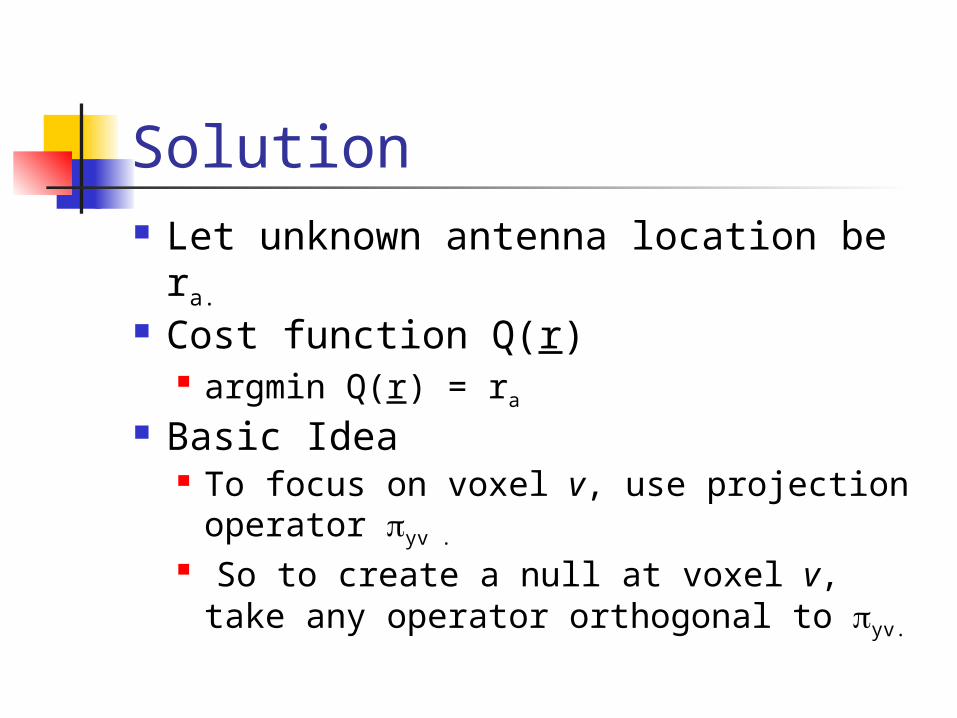
Solution Let unknown antenna location be ra.
Cost function Q(r) argmin Q(r) = ra
Basic Idea To focus on voxel v, use projection
operator yv .
So to create a null at voxel v, take any operator orthogonal to yv.
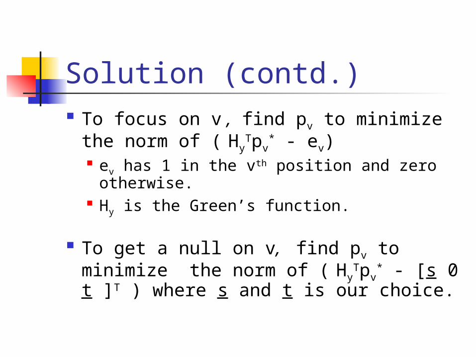
Solution (contd.) To focus on v , find pv to minimize
the norm of ( HyTpv
* - ev) ev has 1 in the vth position and zero
otherwise. Hy is the Green’s function.
To get a null on v, find pv to minimize the norm of ( Hy
Tpv* - [s 0
t ]T ) where s and t is our choice.
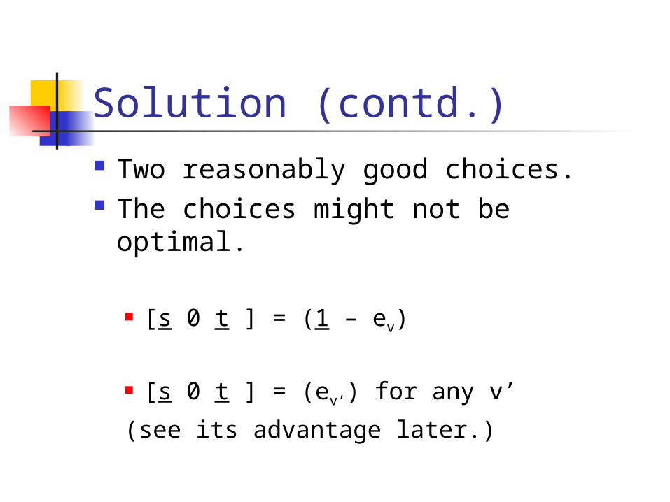
Solution (contd.) Two reasonably good choices. The choices might not be optimal.
[s 0 t ] = (1 – ev)
[s 0 t ] = (ev’) for any v’
(see its advantage later.)
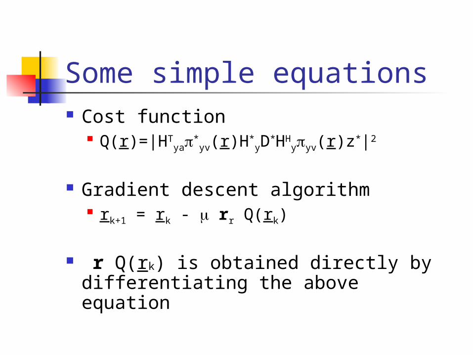
Some simple equations Cost function
Q(r)=|HTya*
yv(r)H*yD*HH
yyv(r)z*|2
Gradient descent algorithm rk+1 = rk - rr Q(rk)
r Q(rk) is obtained directly by differentiating the above equation

Plots

Problems needs to be carefully chosen.
Good initial estimate. Reasonable Assumption.
Problems of local minima(very likely). Solution ?

Momentum Filter
)(
)( )(
1
11
qB
qAqH
)( )( 11 krkk rQqHrr
) - 1 ( )( ; 1 )( -111 qqBqA

More Preliminary Results Comparison with CRB Setting
Set of antennas and voxels. Assume one coordinate of an antenna is unknown.
SNR=10dB. Run over all initial positions in a region R
(in the vicinity of other antennas ) and varying noise.
Focus on some voxel v’
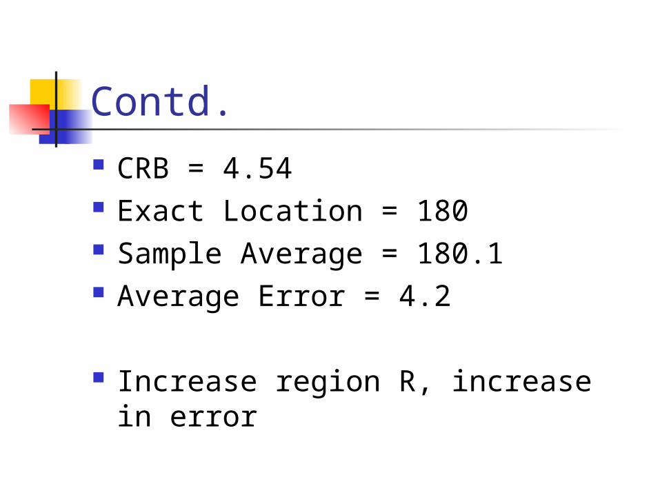
Contd. CRB = 4.54 Exact Location = 180 Sample Average = 180.1 Average Error = 4.2
Increase region R, increase in error
Future work Compare estimators with the CRB. Comparing estimates from TRM with
conventional beam forming methods. Interesting idea
Use focusing on voxel v’ to calibrate antenna position and estimate scattering coefficient simultaneously.
That would be great !
Questions