adaptive and fuzzy approaches for nodes afﬁnity management...

Mobile Information Systems 4 (2008) 273–295 273IOS Press

Adaptive and fuzzy approaches for nodesaffinity management in wireless ad-hocnetworks

Essam Natsheh and Tat-Chee WanSchool of Computer Sciences, Universiti Sains Malaysia, USM 11800, Penang, MalaysiaTel.: +604 653 2062; Fax: +604 657 3335; E-mail: dr [email protected], [email protected]

Abstract. In most of the ad-hoc routing protocols, a static link lifetime (LL) is used for a newly discovered neighbors. Thoughthis works well for networks with fixed infrastructures, it is inadequate for ad-hoc networks due to nodes mobility and frequentbreaks of links. To overcome this problem, routing protocols with estimated LL using nodes affinity were introduced. However,these protocols also used the static estimated LL during the connection time. In contrast to that, in this paper two methods arepresented to estimate LL based on nodes affinity and then continually update those values depending on changes of the affinity.In the first method, linear function is used to map the relationship between the signal strength fluctuation and LL. In the secondmethod, fuzzy logic system is used to map this relationship in a nonlinear fashion. Significance of the proposed methods isvalidated using simulation. Results indicate that fuzzy method provides the most efficient and robust LL values for routingprotocols.

Keywords: Ad-hoc networks, AODV, link lifetime, fuzzy systems, intelligent networks

1. Introduction

Wireless ad-hoc networks consist of mobile nodes and have no fixed infrastructure. The mobilitymakes the nodes continually having new neighbors and losing some others. Each node must have self-detection capability to discover the nodes around it (neighbors) and through them it can reach far nodes(multi-hop concept). Therefore, one of the most concerns of the nodes is to have reliable values for linkslifetime (LL) with their neighbors. If LL is too short, the node will suffer from continually checking theneighbors’ connectivity. On the other hand, if LL is too high, the nodes will suffer from late discoveringof broken links. Therefore, LL value is one of the most important parameters that the designer of ad-hocrouting protocol must takes into account.

To overcome choosing a suitable value for LL, Paul et al. [3] proposed to use the nodes affinity as ametric for LL. The idea behind it is strongly connected nodes must have higher values for LL than weaklyconnected nodes. Using this idea many protocols have been proposed in literature to determine LL valuesbased on signal strength. These protocols outperform traditional protocols with static estimation of LL.However, these protocols use the estimated LL as a static value during the whole connection time. In thispaper, the design and implementation of two adaptive mechanisms are described. They can determinesuitable value of LL based on nodes affinity, and then they continually adapt this value based on changesof signal strength. The first mechanism, called adaptive-LL, optimizes LL linearly and have simpleimplementation. To provide non-linear optimization, fuzzy logic system is used which can provide this

1574-017X/08/$17.00 2008 – IOS Press and the authors. All rights reserved

274 E. Natsheh and T.-C. Wan / Adaptive and fuzzy approaches for nodes affinity management

option effectively, and hence, provide more accurate LL estimation. The second mechanism is calledfuzzy-LL. These two mechanisms help the routing protocols to minimize packet loss while providingreliable LL.

To implement the proposed methods,Ad-hoc On-demand Distance Vector (AODV) routing protocol [1]is utilized as the underlying routing platform. AODV is a reactive routing protocol where the routes aredetermined as per needed only. It manages local connectivity using two parameters: hello intervaland allowed hello loss. The hello interval specifies the time between two Hello messages,usually it is set to 1-second. If a neighbor does not receive any packets (Hello messages or otherwise)for more than allowed hello loss × hello interval seconds, the node should assume thelink to this neighbor is broken. Broch et al. [28] find that using allowed hello loss equal to 3 canproduce best protocol performance. Therefore, LL takes a static value equal to 3-seconds.

Although our proposed methods are evaluated with AODV, they are suitable to use in any other ad-hocrouting protocols as well.

The rest of this paper is organized as follows. Section 2 summarizes related work on using signalstrength to optimize neighbor connectivity. Followed by the implementation of adaptive-LL method,fuzzy-LL method, performance analyzes of the proposed methods, and finally the conclusions.

2. Related work

Dube et al. [2] proposed Signal Stability-based Adaptive (SSA) routing protocol using signal strengthand stability of individual hosts as route selection criteria. According to the signal strength betweentwo neighbors, SSA classifies the link between them as strongly/weakly connected. However, manystudies [3–5] show that discovering a strong link does not necessarily lead to discovering a long lifetimeroute since the other links extending from the end node with the strong link may be very short LL. Toovercome that, Paul et al. [3] introduce a parameter – affinity – which characterizes the relationshipstrength between two neighbors. This parameter utilizes LL as a measure of the strength of link. Theaffinity between two nodes n and m, anm, is:

aam =

{high if ∆Snm(ave) > 0Sthresh−Snm(current)

∆Snm(ave)otherwise

(1)

where Sthresh is the threshold signal strength below which the link will be assumed broken. ∆Snm(ave)

is the average rate of change of signal strength over past few samples, where ∆Snm is defined as:

∆Snm =Snm(current) − Snm(previous)

∆t(2)

Many researchers inherited the concept of affinity in designing their routing protocol. Agarwalet al. [4]proposed Route-Lifetime Assessment Based Routing protocol (RABR), which incorporates the residual-route-lifetime prediction on the basis of affinity appraisal. In addition, the protocol also considered thepath length while choosing an optimal route for a TCP source.

In [6–11], the authors used single to noise ratio (SNR) as a measure of affinity between two neighbors.The authors in [12] used propagation loss factor while in [13,14] used signal strength threshold to achievethe same target. Although those factors are good metrics of nodes affinity, they works at a physical layerof ad-hoc networks and they depends on the antenna and network adapter, hence, they needs interlayer

E. Natsheh and T.-C. Wan / Adaptive and fuzzy approaches for nodes affinity management 275

_

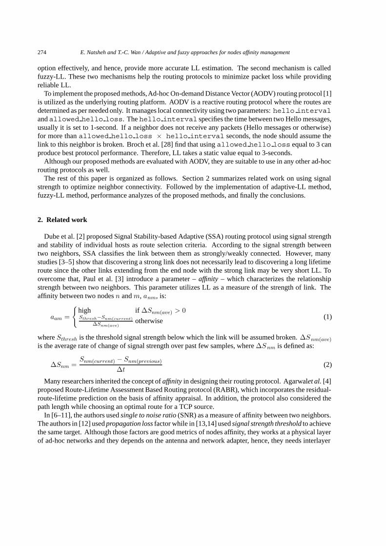
At every ∆t seconds:

Calculate ∆Snm;if (∆Snm > 0 and Link_Lifetime 6)

Link_Lifetime = Link_Lifetime + α; // increment

else if ( Snm < 0 and Link_Lifetime >_

<

0.2)

Link_Lifetime = Link_Lifetime * β; // decrement

Fixed Parameters:

∆t = 0.5 seconds; // sampling interval time.

αβ

= 0.2; // increase factor.

= 0.9; // decrease factor.

Fig. 1. Adaptive-LL algorithm.

interaction with routing layer to choose stable paths. More research is needed to see how the routing layershould use information received from the physical layer and its effect on performance optimization [15].

Other studies used the signal strength fluctuation as an indicator of possible link breakage. In [16], theauthors argue that when signal strength is going to be stronger it means that two nodes will be closer andthe link between them would have longer lifetime. In [17,18], the authors used this concept to suggest analgorithm of early searching for an alternative route when the original route going to be weaker. In [11],the authors exploit the variation tendency of signal strength to detect the relative movement betweennodes, which is utilized to identify leaving and thus unreliable neighbors.

3. Adaptive links lifetime method

Figure 1 presents an on-line algorithm for adaptively changing the LL according to the observed signalstrength. The idea behind this algorithm is to infer whether LL should become longer or shorter byexamining the variations in signal strength. If ∆Snm is positive, it indicates that the affinity is increasingand the signal strength become stronger, then LL should be longer. On the other hand, if ∆Snm isnegative, it indicates that the affinity is decreasing and the signal strength become weaker, then LLshould be shorter.

To ensure that LL will be in acceptable range, we restrict it to stay within the range [0.2, 6] seconds.This ensures the acceptable range of LL, does not matter, whether the signal strength is very weak orvery strong.

In recommending values for α and β, it is needed to ensure that a single variation of signal strengthdoes not result in large variation in LL. We note that it takes at least 30 intervals for LL to increase from0.2 seconds to 6 seconds or to decrease from 6 seconds to 0.2 seconds, which is 15 seconds for ourdefault parameters for ∆t, α and β. More accurate variation of LL could be achieved using non-linearcapability of fuzzy logic method proposed in the next section.

4. Fuzzy logic based links lifetime method

In this section, the proposed concept and rules for fuzzy affinity algorithm, used with AODV areintroduced. In the following subsection, we discuses the need for fuzzy configuration of routingprotocols parameters, followed by three subsections determines the effect of some node parameterson nodes’ affinity. These parameters are then used in subsection E to create the rules of the fuzzy system.


A method to design their membership functions is presented in subsection F. The overall system designis presented in subsection G, followed by the discussion of its compatibility with original static method.

4.1. Fuzzy configuration of routing protocols parameters

In this technique the fuzzy reasoning is used to dynamically configure the protocols parameters insteadof using static values. The dynamical configuration can adapt to the changing of the network topologyand improve the protocol performance. In other hand using static parameters for the protocols in ad-hocenvironment that suffer from frequent change of network topology and different traffic intensity maydegrade the routing protocols performance.

Wang et al. [29] used a fuzzy reasoning to dynamically configure five routing parameters of AODVrouting protocol. They used mathematical models to represent nodes moving mode and their trafficmode. These models were used to categorize the network environments to 9 categorize. The fuzzyreasoning was used to estimate the nodes membership degree in these environments. Depending on thenode membership degree, the values of the protocol parameters are increased or decreased.

Actually, the fuzzy reasoning can be used more effectively to accurately calculate the real values ofprotocol parameters that map the status of the node and its links [30]. We did this to dynamically adaptroutes lifetimes [31], ‘Hello’ messages interval time [32] and active queue management for congestioncontrol [33]. In this paper we apply the fuzzy reasoning to dynamically adapt links lifetime.

4.2. Effect of node transmission power on links lifetime

Transmission power is a main parameter that determines the number of neighbors for nodes in thisproposed ad-hoc network. Transmission power (TrPower) is the strength by which the signal is sent.

Here, signal power degradation is modeled by the free-space propagation model [19], where thereceived signal strength is:

Pr(d) =PtGtGrλ

2

(4π)2d2L(3)

where Pr and Pt are the receive and transmit powers (in Watts), Gt and Gr are the transmit and receiveantenna gains, d is the transmit-receive separation distance, L is a system loss factor (L = 1 in oursimulations which indicates no loss in the system hardware), and λ is the carrier wavelength (in meters)which is related to the carrier frequency (fc) as:

λ =c

fc(4)

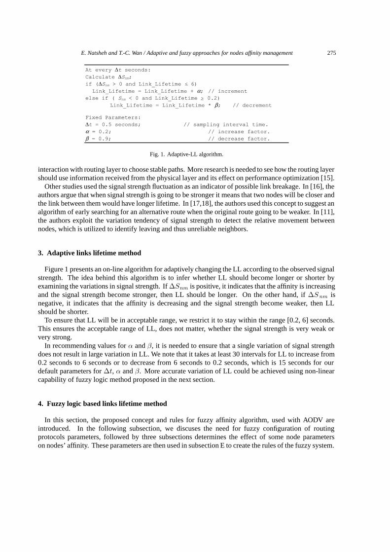
where c is the speed of light (3 × 108 m/s). Assuming a unity gain antenna with a 900 MHz carrierfrequency, Fig. 2 shows the relation between the transmission range (TrRange) and the transmissionpower (TrPower). From this figure, if the TrPower of a node is too low, then the signal will reach to afew neighbors only and the links with those neighbors may be weak and easy to break. Consequently,LL must be small enough to get fast update for neighborhood changes. In contrast, high TrPower ofa node will lead to high average number of its neighbors and hence increase the lifetime of its links,consequently the LL must be long due to fewer changes in node’s neighborhood. Hence the followingrules are proposed:

R1: If DTTRR is high then LL must be low


Fig. 2. TrRange-TrPower relationship.

R2: If DTTRR is medium then LL must be mediumR3: If DTTRR is low then LL must be high

where DTTRR is distance to TrRange ratio. When DTTRR is high that mean the neighbor is far awayfrom the node but it’s still inside the TrRange. In contrast, when DTTRR is low that mean the neighboris near to the node and it’s even closer than the half of TrRange.

4.3. Effect of distance between neighbors on links lifetime

By increasing the distance between a node and its neighbor, the transmission loss or propagation losscan also be increased. For free-space propagation, the loss L f is defined as [19]:

Lf =Pt

Pr=

1GrGt

(4πdλ

)2

(5)

For omnidirectional transmit and receive unity gain antennas, Lf are given by:

Lf =(

4πdλ

)2

=(

4πfcd

c

)2

(6)

Lf in decibels can be written as:

Lf = 32.45 + 20 log10(fc) + 210 log10(d) (7)

Figure 3 shows the propagation loss characteristics. From this figure, it is obvious that if a node havea neighbor and they moves away from each other, then the connectivity strength between them will beweaker and vice versa. Hence, the following rules are proposed:

R4: If ∆d is negative then LL must be highR5: If ∆d is zero then LL must be mediumR6: If ∆d is positive then LL must be low


Fig. 3. Distance-propagation-loss relationship.

where ∆d is the difference between the current neighbor position and its previous position. When ∆d isnegative that means the neighbor becomes closer to the node and, as described above, the connectivitystrength will be stronger. In contrast, when ∆d becomes positive, the neighbor moves away and theconnectivity will be weaker.

4.4. Effect of node speed on links lifetime

Ad-hoc networks experience dynamic changes in network topology because of unrestricted mobilityof the nodes. If a node has fast movement, this leads to an increase in probability of links breaks with itsneighborhood. The node movement can be measured by its speed. High-speed of a node results a highprobability of losing some of the current neighbors and acquiring new ones.

Galluccio et al. [20] calculated the neighborhood time, Tn, between two node n1 and n2 as:

Tn =2 ×

√R2 − P 2

n1

vn1(8)

where R is the transmission range, Pn1 is the position of n1 according to n2, and v′n1 is the relative

velocity and can be calculated as:

v′n1 =√

v2n1 + v2

n2 − 2v2n1v

2n2 cos(Φ) (9)

where vn1 is the magnitude of the vector �vn1, vn2 is the magnitude of the vector �vn2, and Φ is the anglebetween them. Even though the assumption of Tn is accurate only with constant relative velocity, it canshow the effect of nodes’ velocity on neighborhood time (in Fig. 4). From this figure, it is clear that thelinks’ lifetime for fast moving nodes with their neighbors is very small due the expected links breaks.

In general, a rule can be defined as: when speed is high, the LL must be low and vice versa.Consequently the following rules are proposed:

R7: If speed is high then LL must be lowR8: If speed is medium then LL must be mediumR9: If speed is low then LL must be high


Fig. 4. The effect of nodes’ velocity on neighborhood time.

4.5. The rule-base for fuzzy links lifetime

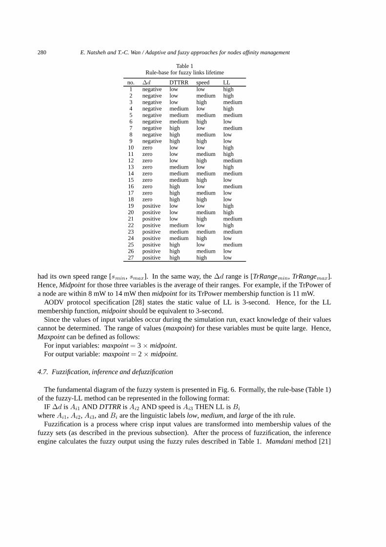
To fulfill the fuzzy sets theory, the previous nine rules (R1 to R9) can be combined within one rule-baseto control the LL adaptively as presented in Table 1. For example, according to Table 1 the first rule is:

IF ∆d is negative AND DTTRR is low AND speed is low THEN LL is high.

4.6. Membership functions for the fuzzy variables

After defining the fuzzy linguistic ‘if-then’ rules, the membership functions corresponding to eachelement in the linguistic set must be defined. For example, if the TrPower equal to 7 mW, usingconventional concept, it implies TrPower is either ‘low’ or ‘medium’ but not both. In fuzzy logic,however, the concept of membership functions allows us to mention the TrPower is ‘low’ with 80%membership degree and ‘medium’ with 20% membership degree.

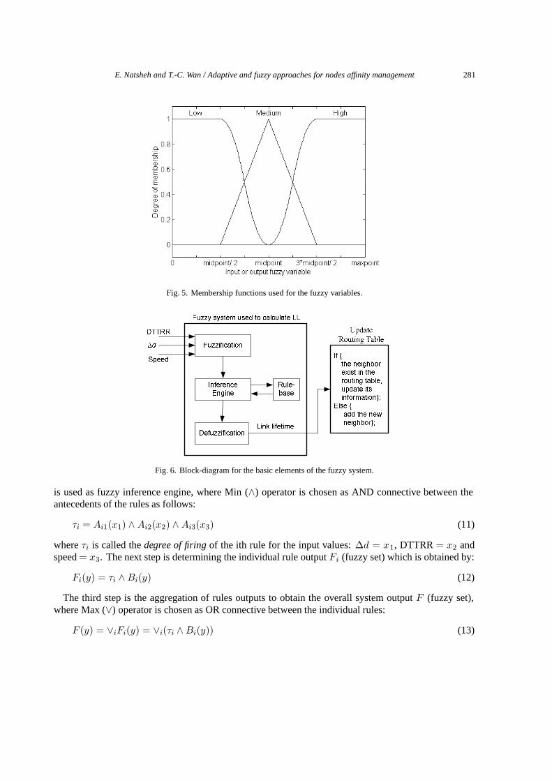
The proposed membership functions are shown in Fig. 5 due to their economic nature of the parametricand functional descriptions. In these membership functions, the designer needs only to define twoparameters; midpoint and maxpoint. These membership functions mainly contain the triangular shapedmembership function. This function is specified by three parameters (a, b, c) as follows:

triangle(x; a, b, c) =

(x− a)/(b− a) for a � x � b(c− x)/(c − b) for b � x � c0 elsewhere

(10)

where a = midpoint/2, b = midpoint, c = 3 × midpoint/2 and x is the input to the fuzzy system. Theremaining membership functions are as follows: Z-shaped membership to represent the whole set of lowvalues and S-shaped membership to represent the whole set of high values.

Midpoint is the value of fuzzy variable, which can be chosen from the real network measurements,simulation and analysis or from the default values of protocol specification as follows.

Normally the TrPower of a node can be read from the properties of the network adapter. So, it is easyto expect the minimum and the maximum TrPower for the nodes sharing the network. Also every node


Table 1Rule-base for fuzzy links lifetime

no. ∆d DTTRR speed LL1 negative low low high2 negative low medium high3 negative low high medium4 negative medium low high5 negative medium medium medium6 negative medium high low7 negative high low medium8 negative high medium low9 negative high high low

10 zero low low high11 zero low medium high12 zero low high medium13 zero medium low high14 zero medium medium medium15 zero medium high low16 zero high low medium17 zero high medium low18 zero high high low19 positive low low high20 positive low medium high21 positive low high medium22 positive medium low high23 positive medium medium medium24 positive medium high low25 positive high low medium26 positive high medium low27 positive high high low

had its own speed range [smin, smax]. In the same way, the ∆d range is [TrRangemin, TrRangemax].Hence, Midpoint for those three variables is the average of their ranges. For example, if the TrPower ofa node are within 8 mW to 14 mW then midpoint for its TrPower membership function is 11 mW.

AODV protocol specification [28] states the static value of LL is 3-second. Hence, for the LLmembership function, midpoint should be equivalent to 3-second.

Since the values of input variables occur during the simulation run, exact knowledge of their valuescannot be determined. The range of values (maxpoint) for these variables must be quite large. Hence,Maxpoint can be defined as follows:

For input variables: maxpoint = 3 × midpoint.For output variable: maxpoint = 2 × midpoint.

4.7. Fuzzification, inference and defuzzification

The fundamental diagram of the fuzzy system is presented in Fig. 6. Formally, the rule-base (Table 1)of the fuzzy-LL method can be represented in the following format:

IF ∆d is Ai1 AND DTTRR is Ai2 AND speed is Ai3 THEN LL is Bi

where Ai1, Ai2, Ai3, and Bi are the linguistic labels low, medium, and large of the ith rule.Fuzzification is a process where crisp input values are transformed into membership values of the

fuzzy sets (as described in the previous subsection). After the process of fuzzification, the inferenceengine calculates the fuzzy output using the fuzzy rules described in Table 1. Mamdani method [21]


Fig. 5. Membership functions used for the fuzzy variables.

Fig. 6. Block-diagram for the basic elements of the fuzzy system.

is used as fuzzy inference engine, where Min (∧) operator is chosen as AND connective between theantecedents of the rules as follows:

τi = Ai1(x1) ∧Ai2(x2) ∧Ai3(x3) (11)

where τi is called the degree of firing of the ith rule for the input values: ∆d = x1, DTTRR = x2 andspeed = x3. The next step is determining the individual rule output Fi (fuzzy set) which is obtained by:

Fi(y) = τi ∧Bi(y) (12)

The third step is the aggregation of rules outputs to obtain the overall system output F (fuzzy set),where Max (∨) operator is chosen as OR connective between the individual rules:

F (y) = ∨iFi(y) = ∨i(τi ∧Bi(y)) (13)


For use in the ad-hoc networks environment a fourth step must be added. A crisp single value for LL isneeded. This process is called defuzzification. Center of area (COA) [21] is chosen as the defuzzificationmethod given in the following:

LL =

∑mj=1 F (yj) × yj∑m

j=1 F (yj)(14)

here yj is a sampling point in the discrete universe output F , and F (yj) is its membership degree in themembership function.

4.8. Compatibility between static and adaptive links lifetime

The proposed two adaptive LL methods are compatible with static-LL method in the sense that a nodethat uses adaptive LL (an “intelligent” node) may communicate with a node that uses static-LL (standardnode), as there are no changes in the control messages format or in the other protocol parameters foradaptive LL methods. However, in a network mixed with intelligent and standard nodes, the intelligentnodes have changeable value of LL and hence provide more reliable links reflects updating topologychanges.

5. Performance analysis of the proposed methods

5.1. Simulation environment

Simulation of the proposed AODV design was done using OMNeT++ version 2.3 with Ad-Hocsimulator 1.0 [22]. OMNeT++ is a powerful object-oriented modular discrete event simulator tool. Eachmobile host is a compound module which encapsulates the following simple modules: an applicationlayer, a routing layer, a MAC layer, a physical layer, and a mobility layer.

Application layer: This module produces the data traffic that triggers all the routing operations. In allscenarios, 7 nodes are enabled to transmit. The traffic was modeled by generating a packet burst of 64packets sent to a randomly chosen destination that stays the same for all the burst length. The rate oftransmission is 3 packets/s. The time elapsed between two application bursts is normally distributed in[0.1, 3] s. The packet size is 512 bytes.

Routing layer: The routing model is the heart of the simulator. This model depicts the AODV routingprotocol, all of its functions, parameters and their implementation [1].

MAC layer: The simple implementation for this layer has been used. The outgoing messages are beinglet pass through. The incoming one instead is delivered to the higher levels with an MM1 queue policy.When an incoming message arrives, the module checks a flag that advises if the higher level is busy. Ifso, the message will be saved in the buffer. If the buffer is full, it will be dropped. When the higher levelis not busy, the MAC module picks the first message from the buffer and sends it upward.

Physical layer: It cares about the on-the-fly creation of links that allow the exchange of messagesamong the nodes. Every time a node moves from its position an interdistance check on each node isperformed. If a node gets close enough (depending on the TrPower of the moving nodes) to a newneighbor, a link is created between the two nodes with the following properties: channel bandwidth is11 Mb/s (IEEE 802.11a) and tolerable delay is 10 µ s. Each node has a defined transmission rangechosen from an uniformly distributed number between [90, 120] m.


Table 2control packets used by AODV

Message DescriptionRREQ a Route Request messageRREP a Route Reply messageRERR a Route Error containing a list of the invalid destinationsRREP ACK a RREP acknowledgment message

Mobility layer: The random waypoint model was adopted for the mobility layer. It is one of themost used mobility model in ad-hoc network simulations. In this model, a node randomly selects adestination. On reaching the destination, another random destination is targeted after 3 seconds pausetime. The speed of movement of individual nodes is between [2, 12] m/s. The direction and magnitudeof movement was chosen from a uniformly distributed random number.

Three different network sizes are modeled: 700 m × 700 m map size with 25 nodes, 35 nodes and800 m × 800 m map size with 45 nodes. Each simulation run takes 300 simulated seconds. Multipleruns were conducted for each scenario and collected data was averaged over those runs.

5.2. Validation of the simulator

Nicola Concer, the creator of Ad-Hoc simulator, proved the validity of the simulator by comparingAODV protocol performance with the performance of the same protocol generated by ns-2 simulator [34].He used some performance metrics to compare between the two protocols performance and found thatthe difference between the results is less than 5%.

5.3. Performance metrics

The following metrics were used for measuring performance:

– Routing Overhead:

Overhead=∑n

i=1Number of SentCtrlPkt by source∑n

i=1Number of received data by destination (15)

where n is number of nodes in the network and SentCtrlPkt is control packets used by AODV anddescribed in Table 2. This metric can be employed to estimate how many transmitted control packetsare used for one successful data packet delivery to determine the efficiency and scalability of theprotocol.

– Average End-to-End Delay: Average packet delivery time from a source to a destination. First,for each source-destination pair, average delay for packet delivery is calculated. Then the wholeaverage delay is calculated from average delay of each pair. End-to-end delay includes the delay inthe send buffer, the delay in the interface queue, the bandwidth contention delay at the MAC, andthe propagation delay.

– Sensitivity to mobility model: In the performance evaluation of a protocol for an ad-hoc network,the protocol should be tested under realistic conditions especially realistic movements of the mobilenodes. We use the following mobility models that represent mobile nodes whose movements areindependent of each other (i.e., entity mobility models concept) [23]:Random Walk (RW): A simple mobility model based on random directions and speeds.Random Waypoint (RWP): A model that includes pause times between changes in destination andspeed. This model has been described in subsection A.


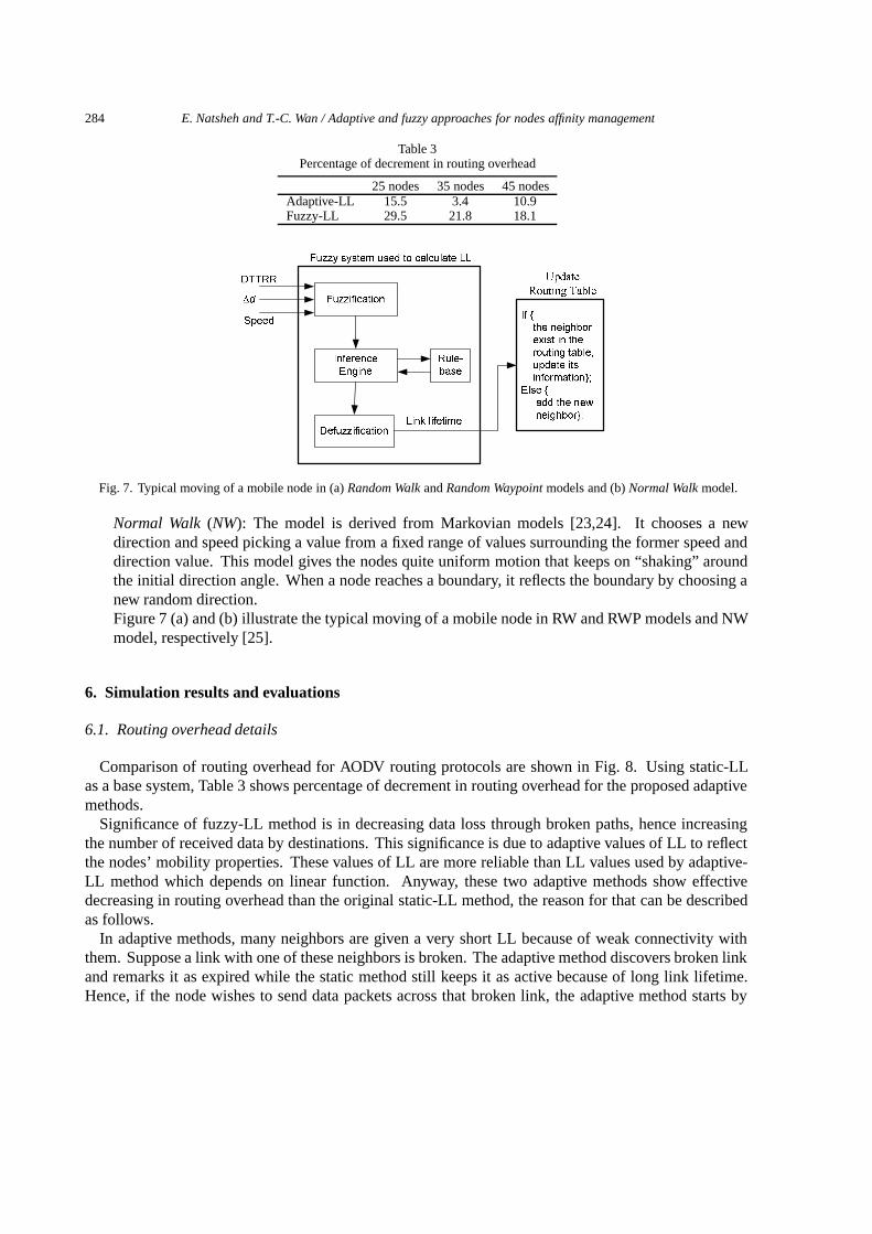
Table 3Percentage of decrement in routing overhead

25 nodes 35 nodes 45 nodesAdaptive-LL 15.5 3.4 10.9Fuzzy-LL 29.5 21.8 18.1

Fig. 7. Typical moving of a mobile node in (a) Random Walk and Random Waypoint models and (b) Normal Walk model.

Normal Walk (NW): The model is derived from Markovian models [23,24]. It chooses a newdirection and speed picking a value from a fixed range of values surrounding the former speed anddirection value. This model gives the nodes quite uniform motion that keeps on “shaking” aroundthe initial direction angle. When a node reaches a boundary, it reflects the boundary by choosing anew random direction.Figure 7 (a) and (b) illustrate the typical moving of a mobile node in RW and RWP models and NWmodel, respectively [25].

6. Simulation results and evaluations

6.1. Routing overhead details

Comparison of routing overhead for AODV routing protocols are shown in Fig. 8. Using static-LLas a base system, Table 3 shows percentage of decrement in routing overhead for the proposed adaptivemethods.

Significance of fuzzy-LL method is in decreasing data loss through broken paths, hence increasingthe number of received data by destinations. This significance is due to adaptive values of LL to reflectthe nodes’ mobility properties. These values of LL are more reliable than LL values used by adaptive-LL method which depends on linear function. Anyway, these two adaptive methods show effectivedecreasing in routing overhead than the original static-LL method, the reason for that can be describedas follows.

In adaptive methods, many neighbors are given a very short LL because of weak connectivity withthem. Suppose a link with one of these neighbors is broken. The adaptive method discovers broken linkand remarks it as expired while the static method still keeps it as active because of long link lifetime.Hence, if the node wishes to send data packets across that broken link, the adaptive method starts by


(a) 25 nodes

(b) 35 nodes

(c) 45 nodes

Fig. 8. Routing overhead comparison.

initiating a path discovery process, while using the static method the node sends the data directly usingthe old broken link. After sending the data, it discovers the broken link, and then the node starts initiatingthe path discovery process.


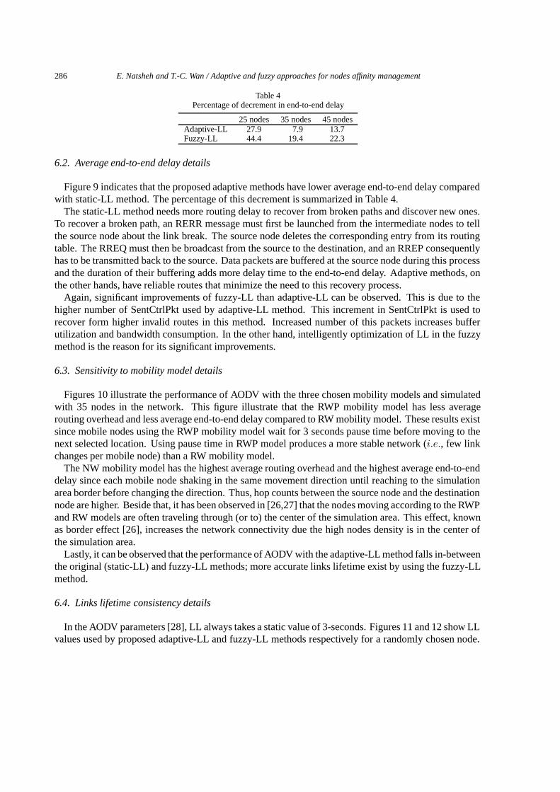
Table 4Percentage of decrement in end-to-end delay


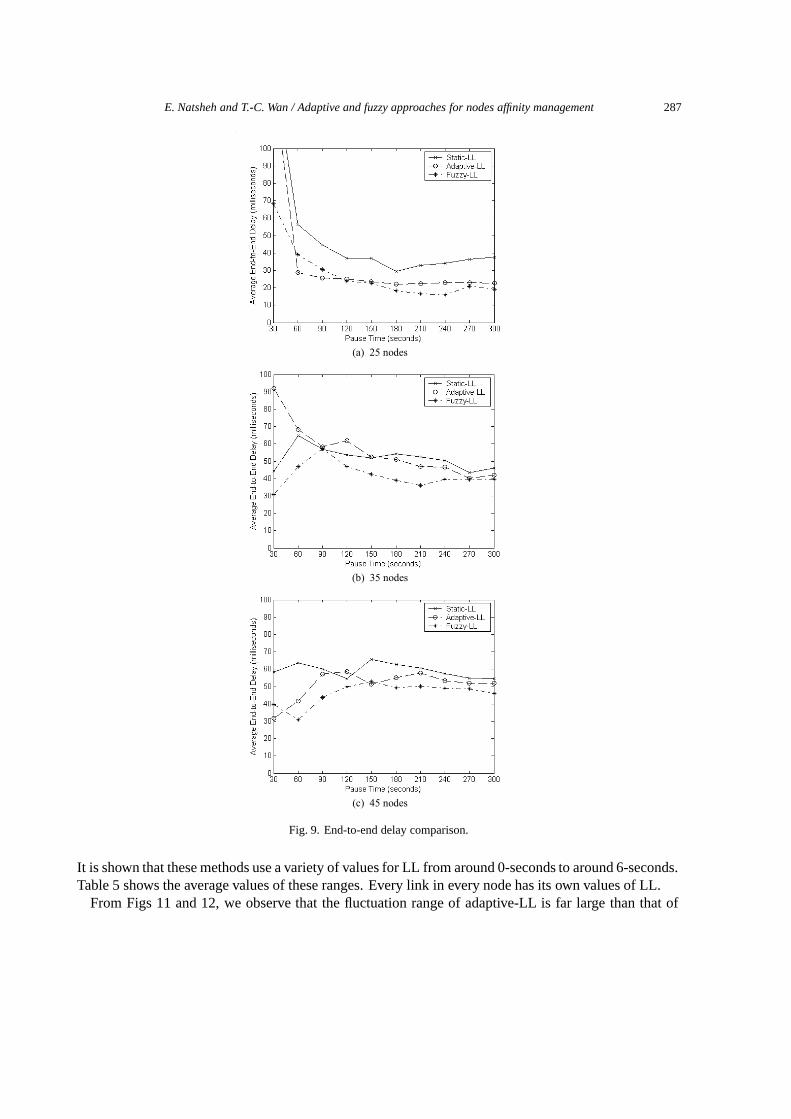
6.2. Average end-to-end delay details

Figure 9 indicates that the proposed adaptive methods have lower average end-to-end delay comparedwith static-LL method. The percentage of this decrement is summarized in Table 4.

The static-LL method needs more routing delay to recover from broken paths and discover new ones.To recover a broken path, an RERR message must first be launched from the intermediate nodes to tellthe source node about the link break. The source node deletes the corresponding entry from its routingtable. The RREQ must then be broadcast from the source to the destination, and an RREP consequentlyhas to be transmitted back to the source. Data packets are buffered at the source node during this processand the duration of their buffering adds more delay time to the end-to-end delay. Adaptive methods, onthe other hands, have reliable routes that minimize the need to this recovery process.

Again, significant improvements of fuzzy-LL than adaptive-LL can be observed. This is due to thehigher number of SentCtrlPkt used by adaptive-LL method. This increment in SentCtrlPkt is used torecover form higher invalid routes in this method. Increased number of this packets increases bufferutilization and bandwidth consumption. In the other hand, intelligently optimization of LL in the fuzzymethod is the reason for its significant improvements.

6.3. Sensitivity to mobility model details

Figures 10 illustrate the performance of AODV with the three chosen mobility models and simulatedwith 35 nodes in the network. This figure illustrate that the RWP mobility model has less averagerouting overhead and less average end-to-end delay compared to RW mobility model. These results existsince mobile nodes using the RWP mobility model wait for 3 seconds pause time before moving to thenext selected location. Using pause time in RWP model produces a more stable network (i.e., few linkchanges per mobile node) than a RW mobility model.

The NW mobility model has the highest average routing overhead and the highest average end-to-enddelay since each mobile node shaking in the same movement direction until reaching to the simulationarea border before changing the direction. Thus, hop counts between the source node and the destinationnode are higher. Beside that, it has been observed in [26,27] that the nodes moving according to the RWPand RW models are often traveling through (or to) the center of the simulation area. This effect, knownas border effect [26], increases the network connectivity due the high nodes density is in the center ofthe simulation area.

Lastly, it can be observed that the performance of AODV with the adaptive-LL method falls in-betweenthe original (static-LL) and fuzzy-LL methods; more accurate links lifetime exist by using the fuzzy-LLmethod.

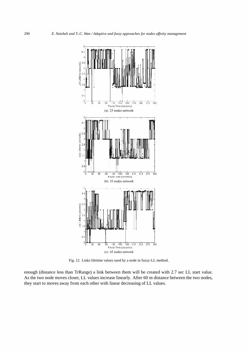
6.4. Links lifetime consistency details

In the AODV parameters [28], LL always takes a static value of 3-seconds. Figures 11 and 12 show LLvalues used by proposed adaptive-LL and fuzzy-LL methods respectively for a randomly chosen node.


(a) 25 nodes

(b) 35 nodes

(c) 45 nodes

Fig. 9. End-to-end delay comparison.

It is shown that these methods use a variety of values for LL from around 0-seconds to around 6-seconds.Table 5 shows the average values of these ranges. Every link in every node has its own values of LL.

From Figs 11 and 12, we observe that the fluctuation range of adaptive-LL is far large than that of


Table 5Average LL values used by a chosen node


(a) Routing overhead comparison

(b) End-to-end delay comparison

Fig. 10. Sensitivity to mobility model comparison.

fuzzy-LL. This makes the fuzzy-LL method more consistent than adaptive-LL method. This is because ithas a nonlinear relationship with the strength of the links as they are weaker or stronger. This consistencyis the accuracy of the proposed mobility measure as the mobility measure reliably represents the linksstrength regardless of network scenarios.


(a) 25 nodes network

(b) 35 nodes network

(c) 45 nodes network

Fig. 11. Links lifetime values used by a node in adaptive-LL method.

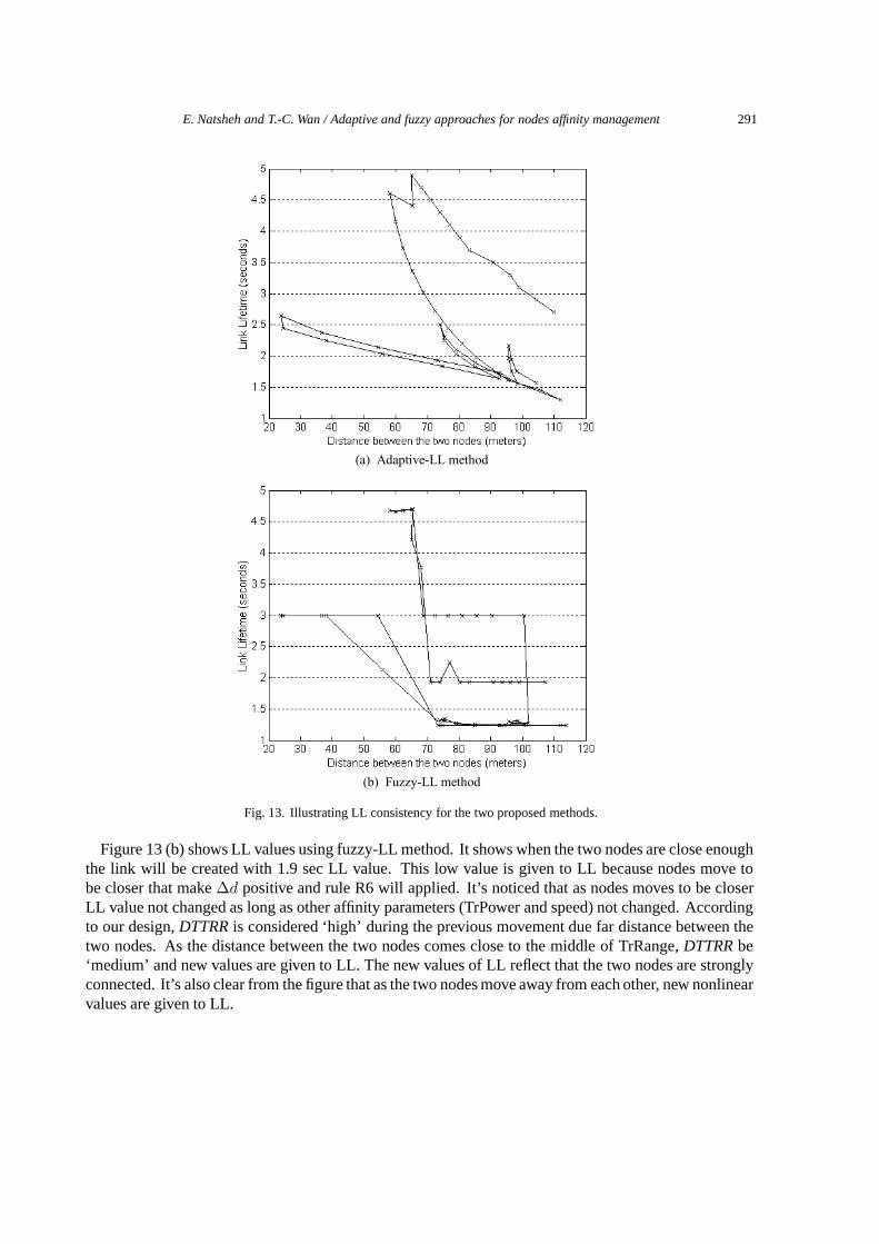
6.5. Illustrating links lifetime consistency

To illustrate LL consistency, we monitor two nodes in our 45 nodes network and record LL values anddistance between them. Figure 13 shows LL values used by the two proposed methods.

Figure 13 (a) shows LL values using adaptive-LL method. It shows when the two nodes are close


(a) 25 nodes network

(b) 35 nodes network

(c) 45 nodes network

Fig. 12. Links lifetime values used by a node in fuzzy-LL method.

enough (distance less than TrRange) a link between them will be created with 2.7 sec LL start value.As the two node moves closer, LL values increase linearly. After 60 m distance between the two nodes,they start to moves away from each other with linear decreasing of LL values.


(a) Adaptive-LL method

(b) Fuzzy-LL method

Fig. 13. Illustrating LL consistency for the two proposed methods.

Figure 13 (b) shows LL values using fuzzy-LL method. It shows when the two nodes are close enoughthe link will be created with 1.9 sec LL value. This low value is given to LL because nodes move tobe closer that make ∆d positive and rule R6 will applied. It’s noticed that as nodes moves to be closerLL value not changed as long as other affinity parameters (TrPower and speed) not changed. Accordingto our design, DTTRR is considered ‘high’ during the previous movement due far distance between thetwo nodes. As the distance between the two nodes comes close to the middle of TrRange, DTTRR be‘medium’ and new values are given to LL. The new values of LL reflect that the two nodes are stronglyconnected. It’s also clear from the figure that as the two nodes move away from each other, new nonlinearvalues are given to LL.


(a) Adaptive-LL method

(b) Fuzzy-LL method

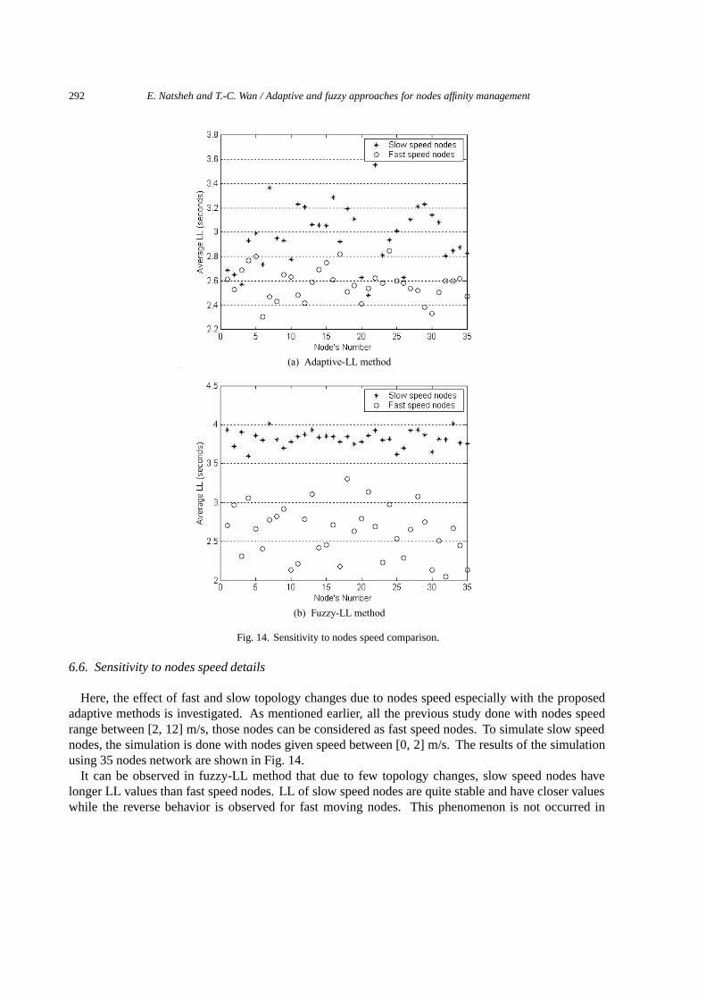
Fig. 14. Sensitivity to nodes speed comparison.

6.6. Sensitivity to nodes speed details

Here, the effect of fast and slow topology changes due to nodes speed especially with the proposedadaptive methods is investigated. As mentioned earlier, all the previous study done with nodes speedrange between [2, 12] m/s, those nodes can be considered as fast speed nodes. To simulate slow speednodes, the simulation is done with nodes given speed between [0, 2] m/s. The results of the simulationusing 35 nodes network are shown in Fig. 14.

It can be observed in fuzzy-LL method that due to few topology changes, slow speed nodes havelonger LL values than fast speed nodes. LL of slow speed nodes are quite stable and have closer valueswhile the reverse behavior is observed for fast moving nodes. This phenomenon is not occurred in


adaptive-LL method. This proves that the signal strength metrics used by fuzzy-LL method reflect anaccurate measure for topology changes. Beside that, the fuzzy engine used in fuzzy-LL method use thestrength of reasoning more optimally than linear functionality used by adaptive-LL method.

7. Conclusions

This paper has shown how adaptive LL can be used to effectively reduce routing overhead and end-to-end delay in ad-hoc networks. To accomplish this, two methods to adaptively optimize LL has beenproposed. The first method (adaptive-LL) used linear function while the second method (fuzzy-LL)used fuzzy reasoning. These two methods maps the relationship between nodes affinity and their LL.Fuzzy-LL method showed more consistency to LL fluctuation and more robust to topology changes thanadaptive-LL method. Experimental results using a small number of nodes have shown the efficacy of thetwo proposed methods. Since LL optimization become more effective as number of nodes increase, it isexpected that the performance will improve significantly as the network grows.

We are currently examining ways to methodically improve the adaptiveness of the ad-hoc routingprotocols. This paper presents adaptation for one specific parameter (LL). There are many otherparameters that can be optimized. For example, route lifetime can actually keep track of the number ofnodes in the path and their affinity changes. In such cases, the protocol should monitor nodes’ affinity totrigger link break notification in time to prevent path loss.

Acknowledgment

This work is partially supported by USM’s project: “Performance Study on Mobile Ad Hoc NetworksRouting Protocols in Heterogeneous Density Environment.”

References

[1] C. Perkins, E.M. Royer and S.R. Das, Ad Hoc On-demand Distance Vector (AODV) routing, Internet-Draft, draft-ietf-manet-aodv-13.txt (Work in progress), Feb 2003.

[2] R. Dube, C.D. Rais, K. Wang and S.K. Tripathi, Signal Stability-Based Adaptive Routing (SSA) for Ad Hoc MobileNetworks, IEEE Personal Communications 4(1) (Feb 1997), 36–45.

[3] K. Paul, S. Bandyopadhyay, A. Mukherjee and D. Saha, Communication-Aware Mobile Hosts in Ad-Hoc WirelessNetwork, Proc of IEEE Int’l Conf. on Personal Wireless Comm (ICPWC) Jaipur, India, (Feb 17–19 1999), 83–87.

[4] S. Agarwal, A. Ahuja, J. Singh and R. Shorey, Route-Lifetime Assessment Based Routing (RABR) Protocol for MobileAd-Hoc Networks, Proc of IEEE Int’l Conf on Comm 3 (June 2000), 1697–1701.

[5] Z. Cheng and W.B. Heinzelman, Exploring Long Lifetime Routing (LLR) in ad hoc Networks, Proc of the 7th ACM Int’lSymposium on Modeling, Analysis and Simulation of Wireless and Mobile Systems Italy, (Oct 4–6 2004), 203–210.

[6] S. Bandyopadhyay and K. Hasuike, A Connection Management Protocol to Support Multimedia Traffic in Ad HocWireless Networks with Directional Antenna, Proc of IEEE Int’l Conf on Multimedia and Expo (ICME2001) Tokyo,Japan, (Aug 2001), 1037–1040.

[7] S. Bandyopadhyay, K. Hasuike, S. Horisawa and S. Tawara, An Adaptive MAC and Directional Routing Protocol for AdHoc Wireless Network Using ESPAR Antenna, Proc of the ACM Symposium on Mobile Ad Hoc Networking & ComputingUSA, (Oct 2001), 243–246.

[8] K.W. Chin, J. Judge, A. Williams and R. Kermode, Implementation Experience with MANET Routing Protocols, ACMSIGCOMM Computer Comm. Review 32(5) (Nov 2002), 49–59.

[9] J. Singh, N. Bambos, B. Srinivasan and D. Clawin, Proposal and Demonstration of Link Connectivity Assessment basedApplications to Routing in Mobile Ad-hoc Networks, IEEE Vehicular Technology Conf 5 Florida, (Oct 2003), 2834–2838.


[10] J. Singh, N. Bambos, B. Srinivasan, D. Clawin and Y. Yan, Empirical Observations on Wireless LAN Performance inVehicular Traffic Scenarios and Link Connectivity based Enhancements for Multihop Routing, IEEE Wireless Comm.and Networking Conf 3 (March 2005), 1676–1682.

[11] J. Liu and V. Issarny, Signal Strength based Service Discovery (S3D) in Mobile Ad Hoc Networks, Proc of the 16thAnnual IEEE Int’l Symposium on Personal Indoor and Mobile Radio Communications (PIMRC), Germany, Sep 2005.

[12] S. Kuo, Y. Tseng, F. Wu and C. Lin, A Probabilistic Signal-strength-based Evaluation Methodology for Sensor NetworkDeployment, Int Journal of Ad Hoc and Ubiquitous Computing 1(1/2) (2005), 3–12.

[13] L. Qin and T. Kunz, On-demand Routing in MANETs: The Impact of a Realistic Physical Layer Model, Proc of the 2ndInt’l Conf Ad Hoc Networks & Wireless (2003), 37–48.

[14] A. Gupta, I. Wormsbecker and C. Williamson, Experimental Evaluation of TCP Performance in Multi-hop Wireless AdHoc Networks, Proc of the IEEE Computer Society’s 12th Annual Int’l Symposium on Modeling, Analysis and Simulationof Computer and Telecommunications Systems Netherlands, (Oct 4–8 2004), 3–11.

[15] J. Lee, S. Singh and Y. Roh, Interlayer Interactions and Performance in Wireless Ad Hoc Network, Internet-Draft,draft-irtf-ans-interlayer-performance-00.txt (work in progress), Sep 2003.

[16] G. Lim, K. Shin, S. Lee, H. Yoon and J. S. Ma, Link Stability and Route Lifetime in Ad-hoc Wireless Networks, Proc ofthe Int’l Conf on Parallel Processing Workshops (ICPPW’02) (Aug 18—21 2002), 116–123.

[17] T. Tien and S.J. Upadhyaya, A Local/Global Strategy Based on Signal Strength for Message Routing in Wireless MobileAd-Hoc Networks, IEEE Academic/Industry Working Conf on Research Challenges 3 (Apr 2000), 227–232.

[18] T. Goff, N.B. Abu-Ghuzaleh, D.S. Phatak and R. Kahvecioglu, Preemptive Routing in Ad Hoc Networks, Proc of the 7thAnnual Int’l Conf on Mobile Computing and Networking Italy, (2001), 43–52.

[19] D.P. Agrawal and Q. Zeng, Introduction to Wireless and Mobile Systems 3 Thomson, (2003), 59–79.[20] L. Galluccio, A. Leonardi, G. Morabito and S. Palazzo, Tradeoff between Energy-Efficiency and Timeliness of Neighbor

Discovery in Self-Organizing Ad Hoc and Sensor Networks, Proc of the 38th Annual Hawaii Int’l Conf on SystemSciences (HICSS’05) 9(9) (2005), 286.1.

[21] R.R. Yager and D.P. Filev, Essentials of Fuzzy Modeling and Control 4 John Wiley & Sons, (1994), 109–153.[22] Available at: http://www.omnetpp.org/.[23] T. Camp, J. Boleng and V. Davies, A Survey of Mobility Models for Ad Hoc Network Research, Wireless Communication

& Mobile Computing (WCMC): Special issue on Mobile Ad Hoc Networking: Research, Trends and Applications 2(5)(2002), 483–502.

[24] D. Shukla, Mobility models in ad hoc networks, Master’s Thesis, KReSIT-ITT, Bombay, Nov 29, 2001.[25] B. Kwak, N. Song and L.E. Miller, A Standard Measure of Mobility for Evaluating Mobile Ad Hoc Network Performance,

IEICE Trans. on Communication E86–B(11) (Nov 2003), 3236–3243.[26] C. Bettstetter, Mobility Modeling in Wireless Networks: Categorization, Smooth Movement, and Border Effects, ACM

Mobile Computing and Communications Review 5(3) (2001), 55–67.[27] C. Bettstetter, G. Resta and P. Santi, The Node Distribution of the Random Waypoint Mobility Model for Wireless Ad

Hoc Networks, IEEE Trans on Mobile Computing 2(3) (2003), 257–269.[28] J. Broch, D.A. Maltz, D.B. Johnson, Y. Hu and J. Jetcheva. A Performance Comparison of Multi-Hop Wireless Ad

Hoc Network Routing Protocols, Proc of the 4th Annual ACM/IEEE Int’l Conf on Mobile Computing and Networking(MOBICOM-98) (Oct 1998), 85–97.

[29] C. Wang, S. Chen, X. Yang and Y. Gao, Fuzzy Logic-Based Dynamic Routing Management Policies for Mobile Ad HocNetworks, Proc of the IEEE Workshop on High Performance Switching and Routing (May 12–14 2005), 341–345.

[30] E. Natsheh, A Survey on Fuzzy Reasoning Applications for Routing Protocols in Wireless Ad-Hoc Networks, Interna-tional Journal of Business Data Communications and Networking (IJBDCN) 4(2) (April–June 2008), 19–31.

[31] E. Natsheh, S. Khatun, A.B. Jantan and S. Subramaniam, Fuzzy Metric Approach for Route Lifetime Determination inWireless Ad-hoc Networks, International Journal of Ad Hoc and Ubiquitous Computing (IJAHUC) 3(1) (2008), 1–9.

[32] E. Natsheh, A.B. Jantan, S. Khatun and S. Subramaniam, Fuzzy Reasoning Approach for Local Connectivity Managementin Mobile Ad-hoc Networks, International Journal of Business Data Communications and Networking (IJBDCN) 2(3)(July–September 2006), 1–18.

[33] E. Natsheh, A.B. Jantan, S. Khatun and S. Subramaniam, Intelligent Reasoning Approach for Active Queue Managementin Wireless Ad-hoc Networks, International Journal of Business Data Communications and Networking (IJBDCN) 3(1)(January–March 2007), 16–33.

[34] Available at: http://www.cs.unibo.it/∼concer/.

Essam Natsheh obtained his PhD in Communications and Networks Engineering from University Putra Malaysia in 2006.Currently, he is an Assistant Professor at the Computer Information Systems Department, College of Applied Studies, KingFaisal University (Saudi Arabia). Beside that, he is doing his post-doctorate research at School of Computer Sciences, Univer-siti Sains Malaysia, in mobile ad-hoc networks, in particular, the development of a new routing algorithm for heterogeneous


density environment. Essam has more than ten years of teaching and research experiences in Malaysia and Saudi Arabia. Al-so, he has published 18 articles in journals and books at international level and over 10 papers in refereed conference proceedings.

Tat-Chee Wan received his BSEE and MSECE from University of Miami, FL in 1990 and 1993 respectively; and his PhD fromUniversiti Sains Malaysia, Penang, Malaysia, in 2005. He is currently Program Chairman for Computer Systems at the Schoolof Computer Sciences, Universiti Sains Malaysia. His research interests include Wireless and Sensor Networks, Multicastprotocols, QoS and embedded real-time systems.

Submit your manuscripts athttp://www.hindawi.com

Computer Games Technology

International Journal of

Hindawi Publishing Corporationhttp://www.hindawi.com Volume 2014


Distributed Sensor Networks


Advances in

FuzzySystems

Hindawi Publishing Corporationhttp://www.hindawi.com

Volume 2014


ReconfigurableComputing

Hindawi Publishing Corporation http://www.hindawi.com Volume 2014


Applied Computational Intelligence and Soft Computing

Advances in

Artificial Intelligence


Advances inSoftware EngineeringHindawi Publishing Corporationhttp://www.hindawi.com Volume 2014


Electrical and Computer Engineering

Journal of

Journal of

Computer Networks and Communications


Hindawi Publishing Corporation

http://www.hindawi.com Volume 2014

Advances in

Multimedia


Biomedical Imaging


ArtificialNeural Systems

Advances in


RoboticsJournal of



Computational Intelligence and Neuroscience

Industrial EngineeringJournal of


Modelling & Simulation in EngineeringHindawi Publishing Corporation http://www.hindawi.com Volume 2014

The Scientific World JournalHindawi Publishing Corporation http://www.hindawi.com Volume 2014


Human-ComputerInteraction

Advances in

Computer EngineeringAdvances in


adaptive and fuzzy approaches for nodes afﬁnity management...

Documents