Adaptation of a reference site selection

methodology to creeks and sloughs of California’s Sacramento Valley and alternative strategies for developing a regional bioassessment framework

Peter R. Ode1, Daniel P. Pickard2, Joseph P. Slusark2 and Andrew C. Rehn1

Report to the Central Valley Regional Water Quality Control Board

March 2005

Aquatic Bioassessment Laboratory California Department of Fish and Game

1Office of Spill Prevention and Response Water Pollution Control Laboratory

2005 Nimbus Road Rancho Cordova, CA 95670

2California State University, Chico

Chico, CA

2

SUGGESTED CITATION Ode, P.R., D. P. Pickard, J. P. Slusark, and A.C. Rehn. 2005. Adaptation of a bioassessment

reference site selection methodology to creeks and sloughs of California’s Sacramento Valley and alternative strategies for applying bioassessment in the valley. Report to the Central Valley Regional Water Quality Control Board. California Department of Fish and Game Aquatic Bioassessment Laboratory, Rancho Cordova, California.

ACKNOWLEDGEMENTS The methodology used in this study was developed through conversations with the Central Valley Bioassessment Committee, whose members have included: Robert Holmes and Jay Rowan (Central Valley Regional Water Quality Control Board), Emilie Reyes (State Water Resources Control Board), Juanita Bacey (Department of Pesticide Regulation), Dan Markiewicz and Kevin Goding (UC Davis Aquatic Toxicology Laboratory), Robert Hall (US EPA), Lenwood Hall (University of Maryland), and James Harrington (Aquatic Bioassessment Laboratory). The methodology presented here was modified from a similar study conducted by Nina Bacey in the San Joaquin Valley. Assistance with site reconnaissance and field data collection was provided by Jennifer York, Jennifer Moore, David Kelly and Ryan Brosius. GIS layers were compiled and modified for this application by DFG’s ITB staff members Will Patterson and Kristina White. Pesticide application data was contributed by Juanita Bacey. Funding for this study was provided by the State Water Resources Control Board through Agreement #01-124-250.

ABSTRACT Bioassessment has shown significant promise as an effective tool for ambient water quality management in many regions of California. However, the scale and intensity of landscape and water transport alteration in the Central Valley pose substantial challenges to implementing bioassessment to its full potential in the region. Bioassessment programs usually are established around a careful characterization of regional reference conditions, which can be defined as the condition of waterbodies that are least impaired by human activities. The reference condition defines a benchmark against which to infer biological impairment and to set expectations for biotic condition. Although there are several techniques available for determining reference condition, by far the most commonly applied is the use of reference sites, which are used to establish the range of natural variability in biotic condition. We investigated the potential for identifying reference sites for segments of sloughs and creeks of the Sacramento Valley at elevations less than 85 meters. We describe here the results of a pilot study designed to adapt an existing reference site selection methodology for use in the Central Valley. Potential reference sloughs and creeks were selected on the basis of a suite of visual assessments of riparian and instream condition and qualitative GIS-based land use data. Analysis of the benthic macroinvertebrate (BMI) assemblages collected from 30 targeted reference sites (23 creeks and 7 sloughs) was focused on addressing two main questions: 1) should creeks and sloughs be considered unique waterbody classes for the purposes of bioassessment?, 2) what is the potential for reference site based bioassessment in valley waterbodies? We addressed these questions with the BMI data using a combination of direct metric comparisons and NMS ordination. To improve our ability to interpret patterns at our 30 sites, we included two additional datasets of BMI data recently collected from nearby waterbodies. We drew three general conclusions from this study: 1) the adaptation of reference site selection to Central Valley streams was effective; we were able to find sites in the valley to use as reference and there is enough diversity in the BMI assemblages at these reference sites to use them to detect impairment, 2) although creeks and sloughs may need to be treated as separate classes of waterbodies for bioassessment-based regulation, there is evidence to suggest that the differences are not clear-cut and the question needs further investigation, 3) BMI assemblages in valley floor reference sites are clearly different from those in foothill reference sites. We discuss the potential for reference site based determination of reference conditions and summarize the current state of the science for defining reference condition in regions without adequate reference sites. We also list a set of recommendations that the Central Valley Regional Water Quality Control Board should consider while constructing a defensible framework for bioassessment in the Central Valley.

3

INTRODUCTION Bioassessment, the science of describing the ecological condition of waterbodies from the assemblages of organisms they contain, is well established as a valuable tool for water resource management (Yoder and Rankin 1995, Karr and Chu 1999, Barbour et al. 1996, Wright et al. 2000, Bailey et al. 2004). When used properly, bioassessments can produce stream condition assessments, set impairment thresholds, monitor effectiveness of restoration projects (Poff et al. 2003), inform the Total Maximum Daily Load (TMDL) process (Karr and Yoder 2004) and help to diagnose sources of impairment. Because assemblages of aquatic organisms (e.g. fish, benthic macroinvertebrates (BMIs) and algae) are comprised of taxa that are differentially responsive to different environmental stressors, bioassessments also provide a direct means of measuring compliance with the goal of biotic integrity stipulated under the Clean Water Act. There are many different approaches to translating a list of organisms present at a site into an assessment of its ecological condition, but the majority establish thresholds of ecological impairment based on a characterization of the taxa expected to occur under minimal human disturbance (Wright et al. 1989, Kerans and Karr 1994, Hawkins et al. 2000, Van Sickle et al. 2005, Ode et al. 2005). As part of this characterization process, traditional bioassessments rely on the concept of the “reference sites” as a benchmark against which to define impairment of ecological condition (Hughes 1995, Reynoldson et al. 1997, Reynoldson and Wright 2000, Bailey et al. 2004). Reference sites are segments of streams (stream reaches) that represent the target state (sensu Meyer 1997) of stream condition for a region of interest. Although there has been much debate about how to define reference condition (Hughes and Larsen 1988, Hughes 1995, Rosenberg et al. 1999, Bailey et al. 2004), the concept is inherently flexible and can be applied either very narrowly (e.g. the condition of waterbodies before European invasions) or more broadly (e.g. the “least disturbed” or “best available” conditions currently found in a region of interest). Thus, the concept of reference condition can be adapted to nearly every situation. The composition of organisms at a site is a function of both natural and anthropogenic factors and both contribute to variability in assemblage composition among sites. Together, these factors can be viewed as a series of “filters” that determine which taxa occur at a site (Poff and Ward 1990, Poff 1997, Statzner et al. 2001). For example, the pool of benthic macroinvertebrate taxa occurring within a large basin like California’s Central Valley is a function of large scale processes (e.g. parent geology, climate and evolutionary history); the subset of taxa that occur at a given site at a given point in time is determined by a series of biotic and abiotic factors (e.g. life history traits, competition and predation, substrate composition, pH, thermal and hydrologic regimes, pollution tolerance) that further limit the occurrence of each taxon. Under this view, the assemblage of organisms collected at a site represents the subset of organisms that passed through all filters. The central challenge in bioassessment is to develop techniques that maximize the detection of signals of anthropogenic stress filters while minimizing the noise from natural filters. The identification of reference sites (which control for sources of variation that are not of interest in monitoring the ecological condition of waterbodies) is a key component of

4

most strategies for meeting this challenge (Hughes 1995, Wright et al. 2000, Bailey et al. 2004). For the past several years, the Central Valley Regional Water Quality Control Board (CVRWQCB) has been investigating the potential for using biological assessment techniques in the waterbodies within its jurisdiction. The majority of worldwide bioassessment methodological research has focused on wadeable streams with gradients steep enough to contain riffle habitats. Although most of the region under the jurisdiction of the CVRWQCB consists of higher gradient systems, much of the CVRWQCB’s regulatory and monitoring focus has been on the low gradient Central Valley ecoregion. While biological monitoring has great potential for water quality monitoring throughout the region, two primary challenges complicate the use of bioassessment as a water quality management tool in the Central Valley (Brown and May 2000, Griffith et al. 2003, deVlaming et al. 2004):

1. Nearly all waterbodies in the Central Valley are subject to highly modified

hydrologies (Domagalski et al. 1998, Domagalski and Brown 1998, Gronberg et al. 1998). California’s Central Valley is one of the most productive agricultural regions in the world and this productivity depends upon an extensive system of natural and modified channels providing water for row crop and orchard irrigation (Domagalski et al. 1998) and intensive application of pesticide, herbicide and fertilizer in order to maintain high crop yields. Even semi-natural waterbodies are subject to water removal and subsidization and inter-basin transfers are common throughout the valley. As a result of these extreme modifications, the standard approach of quantifying land use in the “upstream” watershed is often impossible.

2. Because of its high quality soils, ready supply of clean water and a very long and

predictable growing season, human land use activities have nearly completely altered the natural landscape in the entire Central Valley (Domagalski et al. 1998, Gronberg et al. 1998). Even if one could quantify all the impacts to source water at a site, there are simply very few streams in the region whose watersheds are not greatly modified.

Because this region is so important economically, it has attracted the attention of several exploratory studies undertaken to characterize the benthic macroinvertebrate fauna in the Central Valley including: the multi-agency Sacramento River Watershed Program (SRWP), the US EPA (Central Valley REMAP, Griffith et al. 2003), DOW Chemical Corporation (Hall and Killen 1999), the UC Davis Aquatic Toxicology Laboratory (deVlaming et al. 2004, deVlaming et al. 2005) whose flow was dominated by either agriculture runoff or effluent, the California Department of Pesticide Regulations (Harrington 2004), and the US Geological Survey (Brown and May 2000). These were mostly descriptive studies of relationships among taxa and key environmental factors and contain important characterizations of the BMI assemblages in the Central Valley, but these studies were not intended to set biological expectations for Central Valley waterbodies.

5

If water quality regulators in highly modified regions (e.g. CVRWQCB) are going to use biological data in their assessment programs they will need a formal process for defining impairment thresholds such as could be provided by a characterization of reference conditions. Ode (2002) presented a standardized framework for selecting reference sites developed for higher gradient streams with riffles. The framework was developed using a case study from the Sierra Nevada Foothills ecoregion with funding from the SRWP and the SWRCB. Under this approach, candidate sites are screened through a series of steps to eliminate poor quality sites. GIS landscape analysis is used to identify sites with minimal anthropogenic land use in the upstream watersheds and local reach scale criteria are used to select a final suite of reference sites. Our goal was to see if this approach could be adapted for use in Sacramento Valley streams. Specifically, we were asked to find and characterize 30 reference sites for low-elevation (< 85 meters elevation) creeks and sloughs that were still flowing at the conclusion of the annual irrigation cycle (September-October). It was obvious from the beginning of this study that the standard methodology for characterizing reference condition would need modification to work in this region. This report presents our initial attempts to adapt standardized reference site selection methods for use in Sacramento Valley streams and sloughs. We focused our efforts on three main themes: 1) an evaluation of the potential for reference site based bioassessment in Central Valley waterbodies, 2) a comparison of BMI assemblages in reference creeks and sloughs, and 3) a comparison between reference creeks and sloughs in the Sacramento Valley and reference creeks in the adjacent Sierra Nevada foothills. In addition, since this region does not meet the usual conditions under which bioassessment methods have been developed, the report includes several alternative strategies the CVRWQCB might consider for defining biological expectations for surface waters in the valley floor to support a defensible bioassessment program for the region. METHODS Adapting Reference Site Selection Procedure to Sacramento Valley Streams Original Reference Site Selection Approach The methodology for selecting reference sites developed for the Sierra Nevada Foothill Ecoregion is a five step process (Ode 2002): 1) define the region and waterbodies of interest, 2) use GIS techniques to quantify potential impacts to different areas within the region, 3) identify sampleable stream reaches within least-disturbed candidate areas, 4) use field reconnaissance of candidate areas to eliminate inappropriate sites and obtain site access, 5) apply quantitative local condition assessment to confirm high quality sites. Modified site selection approach The construction of an intensive agricultural irrigation infrastructure has radically altered the original flow patterns in valley watersheds (Domagalski et al.1998). We dealt with this complication by modifying the standard reference site selection approach to de-empha size quantitative land use and emphasize visual assessments of physical characteristics of stream reaches, focusing on reach scale condition, riparian condition, and in-stream physical habitat. The modified process contained 4 steps: 1) define the region of interest

6

and stream classes for evaluation; 2) identify candidate reference reaches using field reconnaissance; 3) use visual assessment data from field reconnaissance in combination with qualitative GIS assessments to screen potential reference reaches, and 4) use quantitative local condition assessments and additional qualitative GIS characterization and to select a final set of the best available sites. Step I: Define the region of interest and stream classes The study region and stream classes were defined for this study by the CVRWQCB to include streams and sloughs under 85 m elevation that were active at the end of the irrigation cycle (i.e. water was either being put into the channel, removed, or both). At the direction of the CVRWQCB, we designated sites as either “sloughs” or “creeks” on the basis of the waterbodies named in the current version of CalWater (version 2.2, Interagency California Mapping Committee 1999, Figure 1). Even though many of these streams are linked by water transport channels, we assumed independence of each water body for the purposes of this study. Step II: Identify candidate reaches In May and June 2004, we conducted an initial round of field reconnaissance to identify stream reaches that were dry or were likely to be dry by the September/ October sampling period and to identify candidate stream reaches for further analysis. General screening with GIS landcover layers (NLCD 2001) was used to eliminate some regions of the study area, but field crews evaluated nearly the entire study region by vehicle-based reconnaissance. Field crews drove through the area to identify stream reaches that met basic criteria for bioassessment sampling (e.g. adequate flow, practical access). Preliminary screening of streams within each target area identified additional regions to be eliminated based on information not available through GIS tools (e.g. local land use activity not recorded in GIS data layers, flow status). After viewing hundreds of potential sampling reaches, we identified 107 candidate sites for further screening. Step III: Screen candidate sites with qualitative GIS and visual habitat assessments Qualitative GIS Assessments We visually assessed the intensity of several key land use activities occurring upstream of each candidate reach: urban/ residential development, total agriculture, orchards/ row crops and total pesticide application (Appendix A). We ranked the intensity of each of these potential impacts for each site at two spatial scales: 1) local activities occurring within a zone approximately 1 km² surrounding the site, and 2) upstream activities occurring within approximately 20 km upstream. Intensity was ranked on a 10 point scale (10 = high intensity). For basic land use data, we used the National Landcover Database (NLCD 2001). The NLCD is based on 1992 LANDSAT satellite imagery and is coded for 21 different types of land use on a 30 meter grid scale. We obtained pesticide data from the California Department of Pesticide Regulation (DPR), which was reported as total lbs. of pesticides applied in 2002 at the section scale (1 mi²).

7

Visual Assessments: We supplemented the GIS analysis with a visual rating of physical habitat condition based on qualitative measures of riparian corridor (width and assemblage), stream habitat (percent channelization, riffle/run/pool sequence, width, and instream substrate), flow regime (channel flow status and obstructions), canopy cover, and crop type and density (Appendix B). Visual assessment scores were scored on a 10 point scale. Scores for each impact were summed for each potential reference site resulting in a site score scale of 0-70. Sites were ranked as Priority I, II, or III, where Priority I sites had cumulative scores of < 25; Priority II sites had cumulative scores of 26 – 50 and Priority III sites had cumulative scores of > 50. Site ownership information was obtained from the County Assessors’ offices and permission letters were sent to owners between June and August. A second visit was made to candidate areas in order to confirm that water was still flowing. At the end of the process we identified 22 potential reference sites that met our criteria and were scheduled for sampling. To increase our sample pool, we repeated the process outlined above. We also revisited candidate sites for which we were denied access and made slight adjustments to sampling locations to accommodate access. This process was repeated until at least 30 potential reference sites were located. These 30 sites were sampled for BMIs and quantitative physical habitat assessments were conducted. Step IV: Select final sites using physical habitat data and GIS To ensure that only the best sites were used for analyses, we performed a final screen of the 30 final sites using the results of the physical habitat data collected at each site with a second round of GIS analysis (Appendix C). We repeated the GIS analyses for the final 30 sites using a more recent landcover dataset (California Department of Forestry and Fire Protection, Multi-source land cover, FRAP) to account for recent changes to local land use. We quantified land use activities occurring within an area 1 km upstream of each site using ArcView® 3.2 software, with the ArcView Spatial Analyst® extension (ESRI Products). For most land use analyses, we used ATtILA, an ArcView extension developed by the EPA’s Landscape Ecology Branch (LEB) in Las Vegas, NV. We removed sites with poor physical habitat characteristics (e.g. poor riparian condition, poor instream habitat, incised channels, a high percentage of fine sediments, hardpan bottoms, poor water chemistry, and low flow). We also eliminated sites that were close to orchards and row crops. After this step, we selected 21 sites as reference and 9 sites were designated as non-reference (3 sloughs and 6 creeks, Appendix D). Benthic Macroinvertebrate Sampling Methodology The wide range of physical habitat conditions and frequent lack of riffle habitats in Central Valley waterbodies prohibits the use of targeted riffle methods like the California Stream Bioassessment Procedure (CSBP) and requires a collection method that can be used equally well for all channel types. We considered three potential sampling methods for use in this study, the three transect low-gradient modification of the CSBP (Harrington 1999), the EPA’s 20 1ft² proportional multiple habitat composite method (Barbour et al. 1999) and the EPA’s EMAP 11 transect reachwide benthos method (Peck et al. 2003). Following

8

discussions with the Central Valley Bioassessment Technical Committee, we used the EMAP reachwide benthos methodology for BMI collection and collected a subset of the standard EMAP field data at each site as follows: Site location was verified with a GPS receiver, sampling time was recorded and digital photographs were taken of the site. Before entering the stream, standard water chemistry measurements (temperature, salinity, dissolved oxygen, and conductivity) were taken with a YSI (Model 85) probe. Alkalinity was measured with a Hach® kit. All sites were assigned a reach length of 150 m, the minimum reach length for EMAP protocol, to reduce problems with private property access. Eleven equally spaced transects (15 m apart) were delineated in each reach. Physical habitat measurements, cross-sectional substrate data, and a benthic macroinvertebrate sub-sample were collected at each transect. Physical habitat measurements included visual riparian estimates, canopy cover estimates (densiometer), fish cover, and human influence. The physical measurements taken at each transect included stream width, five point depth measurements, five point substrate size measurements (pebble counts), substrate embeddedness and bank full width and height. Additional pebble count measurements were made halfway between each transect at five, equally spaced, locations. A 1ft² BMI sub-sample was collected from each of the 11 transects with a 500µ D-frame kicknet and composited into one sample. Stream discharge was measured at each transect using either the velocity area method or the neutrally buoyant object method (Peck et al. 2003). Between each transect, slope and compass bearing were measured. A visual assessment of dominant substrate classes and channel type were recorded for each site. After stream sampling was completed the CSBP rapid habitat assessment form (Barbour et al. 1999) and observed watershed activities for the reach and surrounding area were also recorded. We collected duplicate BMI samples at three of the 30 sites (10%) and processed them along with the other samples. Laboratory Methods Benthic invertebrate samples were processed at the California Department of Fish and Game Aquatic Bioassessment Laboratory (ABL) according to standard operating procedures. California Macroinvertebrate Laboratory Network (CAMLnet) Level II taxonomy (www.dfg.ca.gov/cabw/camlnetste.pdf ) was used for all samples. All samples were subsampled to remove benthic macroinvertebrates from the surrounding detritus until 500 organisms were removed. BMI data were entered into CalEDAS, a Microsoft® Access database application for bioassessment datasets developed by the ABL. Analytical Methods Our analysis of the BMI assemblages collected from the final 30 sites was focused on addressing two main questions: 1) should creeks and sloughs be considered unique waterbody classes for the purposes of bioassessment? and 2) what is the potential for reference site based bioassessment in valley waterbodies? To improve our ability to interpret patterns at our 30 sites, we included two additional sets of BMI data collected recently from nearby waterbodies. In September 2001, BMI

9

assemblages were collected by the ABL from 23 reference sites in the adjacent Sierra Nevada foothills ecoregion (Sibbald et al. 2004). Between fall 2000 and spring 2002, BMI assemblages were collected by the UC Davis Aquatic Toxicology Laboratory (ATL) from 44 sites on 9 agriculture and effluent dominated waterbodies, several of which were identical or similar to those reported in this study (deVlaming et al. 2004). We included both the Sierra foothills data and the ATL data from their fall 2000 sampling event. Data from both of these studies was reported in the original format of the original CSBP (300 count taxa lists from each of 3 transects per site with a total of 900 organisms identified). To permit comparisons among these datasets, we converted each site’s data into single 500 organism count through a Monte Carlo subsampling process (Ode et al. 2005). The CalEDAS database application was used to generate two separate taxonomic lists for each ABL site, calculated at the two standard taxonomic effort levels defined by CAMLnet (www.dfg.ca.gov/cabw/camlnetste.pdf). Level I taxonomic effort (generally genus level taxonomy with chironomid midges identified to family) is the standard taxonomic level used for ambient bioassessment projects throughout California and Level II taxonomic effort (species level IDs when possible, chironomids to genus or species). CalEDAS was then used to calculate 78 BMI metric values for the 30 sites collected for this study at each of the two taxonomic effort levels. Data from the ATL and ABL foothills studies were only analyzed at CAMLnet Level I effort because the original taxonomy was conducted at this level. Once metrics were calculated for all sites, we employed a multi-step process to reduce the number of physical habitat variables to a set of the most informative measures. We reduced the 32 physical habitat measures (Table1, Appendix C) to 19 (Table 1) by removing ones that were highly correlated with each other and by removing measures of fine substrate. The latter were removed because these measures have been linked to the gradient between creeks and sloughs (Cowardin 1979, deVlaming et al. 2005). Thus, when the final set of physical habitat measures was used to screen BMI metrics, we could reduce the influence of metrics that discriminated creeks from sloughs in favor of metrics that discriminated highly-stressed sites from less-stressed sites. After the final set of 19 physical habitat measures was selected, we went through a similar process to screen BMI metrics for suitability in assessing biotic condition of valley floor waterbodies. All 78 metrics were subjected to a screening process that eliminated metrics that either: 1) had insufficient range for scoring, 2) had non-zero values at too few sites to be useful for comparisons, or 3) were unresponsive to the physical habitat stressors we measured. Responsiveness was evaluated with scatterplots of the relationship between metric and stressors and by evaluating correlations between metrics and stressors. As a result of this process, we selected a tightly screened set of 14 metrics (Table 2) that was used to compare among datasets and a more loosely screened set of 36 metrics that was used for NMS analyses. The taxa lists and metrics from the three datasets were divided into five groups for analysis: ABL creeks, ABL sloughs, ABL foothill creeks, ATL high gradient waterbodies (generally creeks) and ATL low gradient waterbodies (generally sloughs). We used two

10

sets of analyses to address the main questions, direct comparisons of metric values among the groups, NMS ordination of both the species and metric data. Direct Metric Comparisons Boxplots were generated for the final 14 BMI metrics to compare sites within each of these groups. The plots were used to make three sets of comparisons: 1) ABL creeks vs. sloughs at Level I taxonomy, 2) ABL creeks vs. sloughs with Level II taxonomy and 3) ABL creeks and sloughs vs. ATL low gradient and high gradient sites vs. foothills reference sites (creeks). Only reference sites were included for the three ABL datasets (creeks, sloughs and foothills). We used t-tests and 2 way analysis of variance (ANOVA) to test for differences between the two waterbody types (creeks vs. sloughs) and between the two datasets (ABL vs. ATL). NMS Species Assemblage NMS - Nonmetric Multi-dimensional Scaling (NMS) is an ordination technique that seeks to explain the variation in species community data in as few dimensions as possible (Kruskal 1964a, 1964b, Mather 1976). We used NMS to explore natural variability in species assemblage composition and variation in BMI metric scores. Species assemblage NMS was performed on Level II taxonomic data for the ABL valley dataset (creeks and sloughs) and on Level I data for both the ABL datasets (creeks, sloughs and foothills) and ATL dataset (low gradient and high gradient waterbodies). The multivariate software program PC-ORD (version 4.0, McCune & Mefford 1999) was used for all NMS analyses. In order to reduce the taxonomic data set for ordination, “parent” taxa were apportioned to their “children” taxa using the US Geological Survey Invertebrate Data Analysis System (version 3.2.6, Cuffney 2003) by distributing ambiguous parent abundance among children in accordance with the relative abundance of each child. Additionally, all taxa that occurred at fewer than four sites were eliminated from the analyses (reducing the Level II dataset of valley floor sites from 200 to 85 taxa and the Level I dataset including foothills sites from 255 to 128 taxa). The following parameters were used in NMS ordinations: distance measure = Bray-Curtis; starting configuration = random; runs with real data = 40; step-down in dimensionality from 6 dimensions to 1 dimension; initial step length = .2; maximum number of iterations per run = 400; stability criterion = .00001; iterations to evaluate stability = 10; Monte Carlo (randomized data) runs = 50. To evaluate associations between environmental variables, we calculated Pearson Product-Moment correlations between NMS axes and physical habitat factors for the ABL valley analysis. Metric NMS- We have observed that variation observed among sites in comparisons of species assemblages is often homogenized when assemblage data is reduced to metric scores (San Diego IBI, ABL unpublished). To investigate the similarity of metric scores among sites, we performed an NMS ordination of 36 metrics screened for range, information content, and responsiveness and using the parameters described for the species ordinations.

11

RESULTS Site Selection and BMI Sampling Based on the initial reconnaissance in May 2004, we identified 107 candidate reference sites: 40 Priority I sites, 60 Priority II sites and 7 Priority III sites. In June 2004, field crews eliminated 41 sites due to poor habitat, uncertain flow status and poor local landscape conditions and an additional 15 sites were eliminated in August and September because the sites were dry. Either because land owners failed to respond to our access request letters or because they denied site access, another 29 sites were eliminated, reducing the number of candidate sites to 22 (12 Priority I sites, 9 Priority II sites and 1 Priority III site). In September 2004, we supplemented the list of sites by screening and selecting an additional 8 sites (see Figure 4 and Appendix A for a listing of the fate of each reconnaissance site). In October and November 2004, the final 30 candidate reference sites were sampled for benthic macroinvertebrates and physical habitat condition and an extensive quantitative GIS analysis of potential reference sites was conducted. We eliminated 9 of the candidate reference based on local land use and physical habitat characteristics of the site (see Appendix C for reasons for elimination of sites). Appendix K contains photographs and full site descriptions of all 30 sites sampled for BMIs. Analytical Results

BMI Assemblage Composition and BMI Metrics Taxonomic lists of benthic macroinvertebrates are presented in Appendices F and G. Lists of metric values for all 78 BMI metrics are presented in Appendices H-K. Metrics Correlations Correlations among physical habitat scores and the 36 BMI metrics that passed the initial range test screens (Table 1) were very similar for the two different taxonomic effort levels. This was also true for the final 14 metrics used for direct metric comparisons. In a few cases (e.g. Alkalinity, Conductivity, Salinity, Percent Irrigated), species level taxonomic effort (Level 2) was more strongly correlated with the environmental variable than was genus level effort (Level I), but this was not true for most variables. Despite an average increase in taxonomic richness at both creek and slough sites of about 50% with increased taxonomic resolution, this did not appear to be associated with increased metric-baseed discrimination of site quality. Responsiveness of Bioassessment Metrics Of the metrics reported as sensitive for San Joaquin Valley waterbodies (deVlaming et al. 2005), only Percent Oligochaeta was responsive in our analysis. Several responsive metrics were related, but not identical to those in the San Joaquin study [Number of Predator taxa (but not Percent Predator Individuals), Percent Collector Taxa (but not Percent Collectors), Percent Non-insect Taxa (but not Percent Insects)]. A few of the San Joaquin metrics were not responsive to the environmental variables we measured [Percent Dominant Taxon, Percent Tolerant and Percent Chironomidae (either genus or family level)].

12

Direct Metric Comparisons ABL creeks vs. sloughs at Level I Taxonomic Effort – These comparisons were based on 4 slough reference sites and 16 creek reference sites. While there were apparent differences between metric values for creeks and sloughs in 11 of the 14 metrics used for screening, with the exception of P_CF_CG_T, P_CG_T and P_TRICHOP (Figure 6, see Table 2 for metric abbreviations), the very small number of reference slough sites limited our power to detect statistically significant differences. Even with this low power, 5 metrics had significantly different scores in creeks and sloughs (EPT_T, N_CF_CG_T, P_EPT_T, P_OLIGO, and RICHNESS, Figure 6, Table 3). The greatest differences between creek and slough values were in EPT_T, N_CF_CG_T, P_NI_T, SHANNON, RICHNESS, and P_OLIGO. Even though there was a clear distinction between the creeks and sloughs in the boxplots, two slough sites (Union School Slough and Willow Slough) had metric values that were similar to those of the creek sites (Appendix H). ABL creeks vs. sloughs at Level II Taxonomic Effort - The pattern of differences between creek and slough metric score distributions was nearly identical for Level II taxonomic effort (Figure 7). As in the Level I comparisons, our low statistical power limited the number of significant different metrics to two (EPT_T and P_OLIGO, Figure 7, Table 3). However, there was a trend toward a greater difference between creeks and sloughs for two metrics (P_CF_CG_T and P_CG_T). This appears to be caused entirely by the addition of taxa when members of the midge family Chironomidae were identified to genus. In the creeks, most of the chironomids were not collector-gatherers, but in sloughs most of them were (e.g. Polypedilum sp., Appendix G). In the Level I dataset, they were only identified to family Chironomidae which is classified as a collector-gatherer at the family level (Appendix F). Scores for the two highest scoring sloughs (Willow Slough and Union School Slough) were again similar to those of the creeks (Appendix I). ABL vs. ATL vs. Foothills - In our comparisons of score distributions of the 14 selected metrics among ABL, ATL, and foothill sites (Figure 8), foothill sites had better metric scores than valley sites in 8 of the 14 metrics, with means often double those of the valley sites (Table 2). In all metrics except for N_DIPTERA_T, P_CF_CG_T and P_CG_T, creeks and sloughs (both valley and foothill) had clearly different metric score distributions. There were no differences among ATL low gradient waterbodies and ABL reference sloughs for any of the 14 metrics (Table 3), except that ATL sloughs were consistently more variable than those of the ABL reference sloughs. Most of the 14 metrics considered here had tight scoring ranges suitable for discriminating between impaired and reference condition at creek sites. The potential for discrimination of reference sites from impaired sites was much lower for sloughs. NMS NMS Species Assemblage ABL Valley creeks vs. sloughs - The NMS ordination of Level II BMI assemblage data from valley creeks and sloughs had a three dimensional optimal solution (final stress = 16.15). Most of the variation in the dataset was accounted for by two axes, Axis 3 (42.7%) and Axis 2 (12.8%). There was a separation between creek and slough assemblages along the minor axis, Axis 2, which accounts for a much smaller

13

amount of the variation among sites (Figure 9, site codes in Table 4). Creeks and sloughs also separated less distinctly along the major axis, but most of this separation was associated with site condition, as reference sites and non-reference sites tended to separate along this axis. This interpretation is supported by the correlations of environmental variables with the two axes (Table 5). The majority of correlations were much stronger with Axis 3 than with Axis 2; this group is primarily comprised of instream habitat and riparian condition measures. There was a second group of variables correlated with the secondary axis that was associated with riparian condition and the overall visual rating of the reconnaissance crews. NMS Valley vs. Foothill Species Assemblages – The NMS ordination of Level I BMI assemblage data from ABL valley sites and ABL foothills sites had a two dimensional solution that explained over 72% of the variation (Axis 1 = 53.6%, Axis 2 = 18.2%, final stress = 19.35; Figure 10). There was a very strong separation of foothills sites from valley sites along Axis 1 (MRRP p<0.00001), with no site showing overlap with valley sites. Interestingly, there was no clustering within the foothills group on the basis of reference status or elevation (Sibbald 2004). Of the valley sites that clustered closest to the foothill sites, five (Comanche Creek (S30, S31), Butte Creek (S50), Hamlin Slough Trib. (S36), Mill Creek (S56), and Toomes Creek (S48)) were sites in Butte and Tehama counties with large, relatively unimpacted upstream watersheds (see Table 6 for site codes). All of the valley sites nested together, with the four reference slough sites falling completely within the creek site group. Of the sloughs, Union School Slough most clearly clustered with creeks, and was closest to the foothill sites. Five sites (Ulatis Creek (S63), Dye Creek (S57), South Honcut Creek (S59), Salt Creek (S38), and Baker Slough (S60)) and fell outside of the clusters of either the valley or foothill reference sites. These five sites were rejected as reference sites based on abiotic factors. Species assemblages at Union School Slough (S23) were more similar to creeks than sloughs. Metric NMS - When the full set of sites (ABL valley and foothill sites, ATL sites) were ordinated on the basis of metric similarity, they exhibited a pattern that closely paralled the result of the species ordination. The NMS ordination resulted in a two dimensional solution in which nearly all the variation in metric scores among sites was partitioned along the first two axes (Axis 1 = 79.4%, Axis 2 = 11.3%, final stress = 14.07; Figure 11). As in the species assemblage data, there was a clear distinction between foothill and valley sites. However, there was considerably more overlap between valley creeks and foothills creeks on the basis of metric similarity than there was on the basis of the species data. Several valley creek sites (Comanche Creek (S34, S35), Butte Creek (S73, S47, S48), Big Chico Creek (S72), and Auburn Ravine-AR4 (S42)) clustered with a group of five foothill sites (Butte Creek RBR (S26), Dry Creek (S12), Deer Creek (S4), Greenwood Creek (S13), and Squaw Hollow (S19) (see Table 7 for site codes). Both Union School Slough (S89) and Willow Slough (S86) again clustered closely with valley creeks and the same five sites rejected for reference again fell outside both the creek or slough reference ellipses. Both ATL low gradient sites and high gradient sites had less within group similarity (as evidenced by the relative sizes of their clusters) than did the equivalent groups of ABL reference sloughs and reference creeks. This pattern was much stronger for ATL low gradient sites than for creeks, which had a very similar distribution to ABL reference

14

creeks. Alder Creek (S36) was a creek site that looked much more similar to sloughs, and was excluded from the creek reference ellipse (Figure 11). Duplicates - The three sites for which we collected duplicate BMI samples for QA/QC purposes had similar positions for each member of the pair in all three ordinations.

DISCUSSION Section 1: Adapting reference site selection to Sacramento River Valley streams The radical alteration of flow patterns to support the intensive agricultural irrigation infrastructure of the Central Valley and the extreme transformation of the valley floor landscape to agricultural and urban uses forced us to identify an alternative strategy for identifying the least disturbed creeks and sloughs in the Sacramento River Valley. We dealt with the complication by modifying the original reference site selection approach to de-emphasize quantitative land use and emphasize visual assessments of physical characteristics of stream reaches, focusing on reach scale condition, riparian condition, and in-stream physical habitat. Using this approach, we were able to identify many good candidate reference sites, close to the number that would be needed to adequately characterize the reference conditions with these sites. We were much more successful at finding reference creeks than we were at finding reference sloughs. Step I: Define the region of interest and stream classes Sloughs vs. Creeks - During the site selection process it became apparent that there is a pressing need for clear definitions for creeks and sloughs in the Central Valley. Although there is general agreement that sloughs are characterized as having lower gradients and having much fewer coarse substrates than creeks, there is a substantial overlap in gradient and instream habitat among waterbodies designated as sloughs or creeks in CalWater 2.2. More critically, there is a continuum of gradient and instream habitat changes that occur in the lower reaches of streams such that there is not a clear point at which creeks become sloughs. In some cases, creeks never become sloughs. These complications raise two questions that must be addressed before bioassessment can be fully implemented in valley streams: 1) is there a sound reason for treating streams and sloughs as distinct habitats (that is, can the least disturbed sloughs and creeks be expected to have similar biotic condition?) and 2) are there consistent physical differences that can be used to define creeks and sloughs? Although we provide evidence in this paper that some sloughs can approach the biotic condition of creeks, we do not have data to adequately answer these questions. In their recent study in the Sacramento River Valley, deVlaming et al. (2004) defined a gradient cutoff of <0.2 percent slope to differentiate between high gradient streams (which generally had hard substrates and roughly equivalent to our creeks) and low gradient streams (which were typically soft bottomed and roughly equivalent to our sloughs). Although there are practical issues associated with the precise measurement of gradient (e.g. is gradient measured at the reach scale or larger scales?, can a waterbody go from a

15

creek to a slough, then back to a creek if the gradient decreases and then increases further downstream?), this could be a useful starting point for defining the classes. A related classification framework for these waterbodies was developed by the US Fish and Wildlife Service for wetlands and deepwater habitats (Cowardin et al. 1979). Under Cowardin’s scheme, there are three waterbody classes of interest in the Central Valley, “Lower Perennial Streams” (systems with minimal surface water, a low gradient, low water velocity, a substrate composition dominated by sand and fine sediments and subject to periodic oxygen depletion), “Upper Perennial Streams” (systems with significant surface water flow, high gradient, fast water velocity, and an unconsolidated substrate of rock, cobble, or gravel with patches of sand) and “Intermittent Streams” (channels containing flowing water for only part of the year). Although we excluded intermittent streams from this study, they are potential subjects for bioassessment monitoring. We encountered an additional stream type in the Sacramento Valley that does not fit easily into this framework. These streams can have the characteristics of an upper perennial stream or lower perennial stream but have hardpan bottoms. Hardpan has the appearance of sandy cobble but is a natural “concrete-like” geologic formation of volcanic origin. This substrate provides little instream habitat and may possess low diversity BMI communities even under pristine conditions. Step II: Identify candidate reaches Under the reference site selection method developed for high gradient streams, candidate regions were pre-screened on the basis of available GIS datasets. The problems with hydrology required us to de-emphasize GIS data in favor of visual screening of candidate areas. We were able to identify several good candidate regions, but improvements in two key areas could greatly improve this step. Perhaps the greatest current impediment to bioassessment statewide is unrestricted access to potential sampling sites. Access restrictions caused by landowner ambivalence or denial impairs our ability to objectively define reference conditions because we can never be certain that we are sampling the full range of conditions. Exacerbating this problem, the lack of access is often greatest in the regions with the best potential for having reference sites. In this study, our attempts to identify good candidate areas were limited to areas that could be evaluated from the road. Thus, potential regions that did not have good road access could easily have been missed. This could be improved with better coordination with local watershed groups and agricultural coalition groups and inclusion of aerial photography. One of the most important technical priorities remains improving GIS datasets and the analytical tools. There is a great need for techniques for quantification of hydrologic modification (Richter et al. 1996) and modeling hydrologic stress (how much alteration from the natural flow regime is a site subject to). Richter’s approach involves the development of Indicators of Hydrologic Alteration (IHA, Richter et al. 1996). We also need a better way of identifying source of water flowing through a reach and a flow model for predicting when natural reaches should be dry. The utility of existing GIS hydrography datasets for Central Valley waterbodies could be greatly improved by linking existing information about channel characteristics to the current hydrography layers (NHD,

16

CalWater). For example, segments of waterbodies could be coded for physical structure (e.g. natural, channelized, artificial-sided, artificial-bottomed), direction of water flow, source water (natural or supplemented), flow duration (seasonal vs. perennial). This information would be a great improvement over existing layers and would allow future researchers to locate candidate reference areas more efficiently, reducing the need for extensive field reconnaissance and increasing our ability to standardize the way these characteristics are reported. Step III: Screen candidate reaches with visual assessments and GIS Qualitative GIS assessments - We scored sites for local and upstream presence of urban and agricultural land use and total reported pesticide loads. These impacts were estimated at a very coarse level and could be improved with better characterization of specific crop and pesticide types. Visual assessments - Our heavy reliance on field reconnaissance limited our ability to screen all potential reference sites because we were only able to survey areas that could be evaluated from public road ways. Other potential sources of screening information – We made no attempt to include existing chemical and toxicological data in our reference site screening process, but this would be a valuable step to add to future investigations (see recommendations in deVlaming et al. 2004). Another good candidate for future studies is the quantification of defunct mining operations in the Sierra Nevada foothills. Contaminants from old mining operations and legacy mercury from gold mining operations may have a significant effect upon water quality. Step IV: Select final sites using physical habitat data and quantitative GIS Collection of physical habitat and BMI data - In addition to the data that were collected here, future attempts to identify reference sites should consider including water and sediment samples with BMI samples to improve the final screening step. Quantitative GIS - Although bioassessment is generally limited by the quality of available GIS land use datasets, accurate quantification of stressors in Valley streams is limited to a far greater degree by the lack of information about the area affecting the source water to each site. Although only 21 sites passed all of the screening steps in this project, some of these are likely unsuitable as reference sites because of factors that we did not account for in this study. The results presented here are therefore conservative in the sense that they understate the biotic potential of reference sites in SVR creeks and sloughs. Section 2: Analytical Results Did reference site selection process work? The adaptation we used for identifying reference sites in valley streams was effective: we identified 21 sites on separate waterways in the Sacramento Valley that could be

17

considered reference quality. With better access permission, this number might easily be doubled. However, the method was slow, requiring substantial amounts of field reconnaissance, and undoubtedly resulted in the inclusion of some poor quality sites. The process was also much more effective at finding high quality creeks than high quality sloughs. There is some evidence from the NMS metric ordination that the creeks and sloughs that passed our reference screens were more similar to each other than to all creeks and sloughs, a condition necessary for bioassessment. There was a large amount of overlap between our creek sites and the high gradient sites studied by the ATL. With the exception of Coon Creek, we collected reference samples from all the ATL waterbodies used for its high gradient samples (Auburn Ravine, Butte Creek, and Dry Creek). Thus, all of high gradient waterbodies analyzed by the ATL were located on creeks that we determined to have at least some reference sites (although the locations within each creek were not the same). In addition to these creeks, we identified 10 other waterbodies (Mill Creek, Deer Creek, Big Chico Creek, Comanche Creek, a creek tributary to Hamlin Slough, Gold Run Creek, Putah Creek, Cache Creek, and Toomes Creek). This similarity did not apply to comparisons between ATL low gradient sites and our reference sloughs. There was much more variation among ATL’s low gradient sites than among our four reference slough sites and the reference sloughs were nearly as similar to other creek sites as they were to all low gradient sites. In order for bioassessment techniques to be successfully applied in valley waterbodies, there must be enough diversity at reference sites to permit the discrimination of impairment. The distribution of scores for most metrics was narrow enough to use them for discrimination of impairment in creeks. This was less true for slough sites; in most cases, metric scores for reference sloughs were likely to be too low to be able to discriminate impairment. DeVlaming et al. (2004) described a similar concern for their low gradient sites. Should creeks and sloughs be treated separately? DeVlaming et al. (2004) presented evidence that high gradient sites (creeks) and low gradient (sloughs) waterbodies have different assemblages and argued that they should be dealt with separately in bioassessment analyses. Although the data presented here give some support to their contention, we believe that the evidence is ambiguous enough that the question needs further exploration. The difficulty in finding good sloughs makes it difficult to answer this question well. We presented evidence here that at least some sloughs have biotic potential similar to that of creeks, but we were only able to identify a handful of slough sites that met our screening criteria. Thus, we do not have enough sites to make strong conclusions about the nature of BMI assemblages at reference sloughs. Direct metric comparisons indicated large differences among sloughs and creeks, regardless of level of taxonomic effort (12 of 14 for Level I, all 14 for Level II). However, the differences between creeks and sloughs were even stronger with Level II comparisons,

18

in which the Chironomidae were identified to genus. The collector-gatherer midges which were found predominantly in sloughs (e.g. Polypedilum sp. and Chironomus sp.) were replaced by other functional feeding groups in creeks. Of the slough sites, Union School Slough and Willow Slough tended to score better than the others, usually falling within the range of creeks. This pattern was repeated in almost all of the metrics. Creeks and sloughs clustered separately in NMS ordinations of both metrics and species assemblage, although there was some overlap among the best sites. When we included the foothills creeks and ATL sites in our NMS analyses, we noticed an interesting effect: although we could detect the separation between creeks vs. sloughs when we looked at them alone or with the other datasets, the differences were much less obvious in the context of the foothills scores. Union School Slough and Willow Slough consistently were associated more closely with creeks than with sloughs in these analyses. Union School Slough has a complete and intact riparian zone, and a relatively good instream habitat, while Willow Slough has good instream habitat, but lacked a complete riparian zone. Instream and riparian habitat were both correlated with the main axis in NMS ordination of the valley creeks and sloughs (Table 5). Taken together, this evidence indicates that at least some sloughs can look similar to creeks, and suggests that sloughs with good instream and riparian habitat may have biotic potential equivalent to that of valley creeks. Because at least some of the slough sites seem to be able to support relatively rich creek-like faunas, we argue that it is premature to decide whether to treat sloughs and creeks as separate waterbody classes for valley floor bioassessments. How do the best valley floor sites compare to foothills sites? Most of our analyses indicate that foothill sites support assemblages that are distinct from those of valley sites. This is true to a lesser degree for similarity based on metrics than it is for species composition. All of the direct metric comparisons (Figure 8) show separation except for number collector-filterer/collector-gatherer taxa, percent collector-gatherer taxa, and percent Ephemeroptera. With these three metrics, scores for valley creeks overlap with those of foothill creeks. The NMS species assemblage data (Figure 10) shows complete separation between valley and foothill sites. All the valley sites that fall out closest to the foothills are Butte and Tehama county sites with large, relatively undisturbed watersheds above the valley sampling location. With the NMS metric data there is still good separation between the valley and foothill sites, but there is more overlap among the Butte and Tehama County sites (Figure 11). These sites are near the 85 m upper elevation threshold for the valley study, and suggest there may be a transition zone between foothill and valley sites near this elevation. Species vs. genus level taxonomic effort Based on the analyses presented here, there is strong evidence that Level I and Level II taxonomic effort would give equivalent interpretations of biotic condition in Valley sites. However, we recommend that bioassessment studies in Central Valley waterbodies should continue to collect species level data (Level II) until we learn more about the impacts of species specific tolerance values on interpretation of biotic condition. As others have stated (deVlaming et al. 2004), it is much easier to collapse species data to genus data than to go back to archived samples to re-identify taxa to a more precise level.

19

Section 3: Alternative Strategies for Central Valley Bioassessment Over the last decade, many of California’s State and Regional Water Quality Control Boards (RWGCBs) have adopted increasingly sophisticated and comprehensive bioassessment programs for their surface water ambient monitoring program (SWAMP). Traditional bioassessment methods (in which biotic impairment is defined relative to a reference condition established from a set of reference sites) appear to be well-suited for measuring biotic integrity in the wadeable streams of these regions. Over the past few years, the SWRCB and CVRWQCB have invested resources to explore bioassessment approaches that will work in the challenging environment of California’s Central Valley. While other regions in California have at least a few watersheds with low gradient streams and highly modified landscapes and hydrologies, the scale of modification present in the Central Valley makes it a good testing ground for alternate methods for measuring biotic integrity. The results of this and other recent studies clearly demonstrate that surface waters in the Sacramento Valley can support rich macroinvertebrate assemblages at some sites, even under considerable alteration and agricultural development (Griffith et al. 2003, deVlaming et al. 2004, deVlaming et al. 2005). This indicates that there is enough range in biotic condition in valley waterbodies to differentiate degrees of impairment. The challenge is to develop a method that will allow the board to set expectations of biological condition and to differentiate degrees of biotic impairment. The challenge of developing sound bioassessment programs in regions without easily identified reference sites is not unique to the Central Valley waterbodies. Researches have developed or are currently developing methods for agricultural areas in the mid-western US (Whittier and Rankin 1992, Yoder and Rankin 1995), large rivers (Robert Hughes personal communication), Australian coastal streams and rivers (Chessman and Royal 2004) and highly urbanized streams in the San Francisco Bay region (Carter and Fend 2005). The following section summarizes a set of three alternative strategies that could be pursued by the board. Each has advantages and potential issues that would need to be overcome. We have attempted to summarize the positions of the practitioners of these approaches and do not necessarily advocate all of these positions. We are presenting these with the intent to generate discussion within the SWRCB and CVRWQCB and its technical advisors. Note that the three alternative strategies are not necessarily mutually exclusive, although they have been presented as distinct strategies in the literature. Alternative I: Continue to identify reference sites using traditional approaches Although our attempt to modify traditional screening methods for identifying reference sites was impaired by several factors, we were successful in finding nearly 20 reference creeks in Sacramento Valley. While we have not identified enough reference sites to construct a Central Valley IBI in the near future, this goal may still be feasible with better strategies for stressor quantification and especially for improving site access.

20

Also, while dozens of reference sites are desirable for good reference condition characterization, practitioners of predictive modeling techniques have argued that O/E models require fewer reference sites for reference condition characterization (Charles Hawkins, personal communication). This may also be true for IBI development: although we generally try to use at least 25 reference sites, IBIs could be developed with many fewer. In either case, the impact of basing models on fewer reference sites would be a reduced ability to discriminate impaired sites from reference sites. Predictive models (e.g. RIVPACS models) use multivariate statistical techniques to generate a list of taxa that are “expected” (=”E”) to occur at a site under reference conditions. The assemblage of taxa observed (=”O”) at a site is compared to the expected assemblage to generate an “O/E” ratio that indicates the degree to which a target site differs from the reference state. Since the reference state has known statistical properties, biotic impairment at a test site can be defined as a specific degree of deviation from the reference state (O/E ratio of 1.0). Discriminant Function Analysis (DA) is used to classify sites according to key factors that are minimally influenced by anthropogenic stresses. These classes partition the variation in BMI assemblages due to natural factors and allow the derivation of probabilities of occurrence for individual taxa that are sensitive to these sources of variation. Although the exact number of reference sites needed to create a stable RIVPACS model for the Central Valley is not yet known, it is technically possible to develop a usable RIVPACS model that has as few as 5 or 6 (Charles Hawkins, personal communication). Another related option is to take advantage of an opportunity to include Central Valley reference sites in the new statewide RIVPACS model that is being proposed for California. The model will be developed by DFG-ABL and the SWRCB (in collaboration with EPA and Charles Hawkins) and will provide a tool for measuring impairment of biotic integrity that can be used throughout the state.

Advantages and Disadvantages: The main advantage to sticking with this approach is that once enough reference sites have been identified with this process, the techniques for developing bioassessment tools are well-established. The primary disadvantage is that any reference conditions developed using this approach will necessarily include a significant degree of human modification, potentially confounding interpretation of any deviation from the reference state. Thus, assessments based on human influenced reference sites will under-represent the degradation due to anthropogenic stresses. What’s Needed: More reference sites will be needed for construction of either a Central Valley IBI or RIVPACS model. The CVRWQCB should take advantage of upcoming efforts to develop a statewide predictive model by collecting data that could be included in the model and improve its applicability to Central Valley streams.

21

Alternative II: Define reference conditions without reference sites A general difficulty with using reference sites to define reference conditions in highly modified regions is well stated by Chessman and Royal (2004): “because the impact at reference sites is often ill-defined, the meaning of a given departure from the reference condition may be ill-defined”. To avoid this problem, Chessman and Royal (1995, 1999, 2004) recently presented an approach to defining reference condition that does not rely on the use of reference sites. The approach has attracted a considerable amount of interest in the applied stream ecology community and the general topic is the subject of a special session at the 2005 annual meeting of the North American Benthological Society. Although the mechanics of this approach are still being developed, its scientific foundation is deeply rooted in ecological theory, particularly in niche theory (Hutchinson 1957) and the “habitat templet” framework (Southwood 1977). More recently, Poff (1997) built on this framework with a heuristic model for predicting the distribution of stream organisms based on an understanding of how different scales of habitat features (e.g. climate, channel morphology, water chemistry, substrate characteristics) act as “filters” that select for particular species traits. This conceptual framework provides a way of accounting for the influence of both natural and anthropogenic factors on species distributions. Chessman and Royal’s solution is to apply Poff’s framework to the problem of determining reference condition without using reference sites. In Chessman and Royal’s application, the tolerance or preference of individual taxa for key environmental filters (e.g. water temperature range, substrate composition, flow regime) is assessed for BMI fauna within a region. These preferences are used to predict the assemblage of taxa that could be expected to occur at any test site under minimal human stress. Deviation from that expectation is used to infer degradation just as it is in predictive models (e.g. RIVPACS, AusRIVAS). This is a very promising approach: even the primitive assignment of taxa to simple preference classes used by Chessman and Royal (2004) resulted in stronger associations between their water quality assessments and independent measures of human disturbance than did the Australian predictive models developed from reference sites. There is some question, however, whether this was a result of a flaw in the predictive model rather than a failure of the reference approach. In any case, the performance of this approach could be much improved by better quantification of species optima/ niche breadth such as is currently being developed for temperature, fine sediments and conductivity (A.C. Rehn unpublished data, L. Yuan unpublished data). Additionally, models of species-environment relationships could be greatly improved by modeling the probability of occurrence of different taxa along specific stressor gradients. This is being explored currently by US EPA in collaboration with Australian national bioassessment programs. This is likely to provide information that would be useful to Central Valley bioassessment programs (L. Yuan personal communication).

Advantages and Disadvantages: This approach promises to circumvent the problem of having too few reference sites by looking at faunistic environmental preferences directly rather than indirectly. If current

22

attempts to improve this method are productive, this may be a good long-term strategy for Central Valley bioassessment programs. What’s Needed: Need to develop models for the environmental affinities of Central Valley fauna. It will take some investment of time and money to collect enough samples to characterize individual BMI responses across key environmental gradients. Some of this data has already been collected and could be explored to identify data gaps. Alternative III: Relax the restriction against using biological information to identify least impaired sites Another general solution to the problem of identifying appropriate reference sites is to relax the philosophical proscription against using biological information to identify reference sites. While this may seem to violate the scientific prohibition against circular reasoning, there are some attractive reasons to investigate this approach and there are techniques to minimize problems with circularity. Factor-Ceiling Approach Like Chessman and Royal, Carter and Fend (2005) counsel against using reference sites to define the reference state in highly modified regions. Because the biotic potential of sites is often limited by the confounding effects of multiple stressor gradients, setting expectations for biotic condition is nearly impossible. Also, the massive degree to which urbanized (or agricultural) watersheds are physically modified limits our ability to distinguish water quality impairment from physical impairment. Since many of the factors controlling physical impairment are not likely to change without wholesale changes in societal priorities, failure to allow decoupling of these factors will limit our ability to document biotic impacts from changes in water quality management practices in these regions. To deal with the difficulties of finding appropriate reference sites in a highly urbanized watershed in the Santa Clara valley, Carter and Fend developed a technique for defining a range of biotic expectation that takes into account the decrease in biotic condition caused by physical modification along an axis of increasing urbanization. The technique involves plotting a relationship between a primary stressor gradient (in their case % urbanization) and various measures of biotic condition (e.g. standard bioassessment metrics). A simple statistical technique (partitioned least squares regression, OLS) is used to identify the highest biotic scores along the entire urbanization gradient. These upper values then define the range of expected biotic conditions for the region. The range of expected biotic response generated from this technique is analogous to that created using the “least disturbed condition” concept of reference sites (Hughes 1995). Since a full urbanization gradient is used to take into account decreasing biotic potential with increasing urbanization, the resulting range of expected conditions is a conservative estimate of biotic potential for the region.

23

Circularity and the “factor-ceiling” – Because biotic response metrics are used directly to identify the best sites, use of the biotic condition of these sites to set biotic expectations for the region is circular. Under most conditions, this violation would cause us to reject this technique because circular reasoning increases the risks of bad conclusions about water quality being made from inappropriate assumptions about relationships between biotic metrics and important stressors. However, the extreme lack of reference sites in the region requires us to consider accepting some circularity while adding additional steps to guard against the risks of circularity. The best way to guard against these risks is to use independent datasets to select the biotic response metrics. Careful selection of metrics using independent datasets can ensure that the metrics are responsive to the stressors of interest to WQ management and regulation. Also, some have argued that the circularity concern is less of a problem in highly modified systems than more pristine systems because relationships between metrics and stressors are simpler (Karr and Chu 1999). Adapting factor-ceiling to Central Valley Ag-dominated Systems- The effects of urbanization on biotic integrity has received a great deal of attention in the bioassessment literature over the last decade (Arnold and Gibbons 1996, Booth and Jackson 1997, Paul and Meyer 2001, Wang et al. 2001). Although less attention has been given to dealing with highly modified agricultural regions (but see Wiley et al. 1990, DeLong and Brusven 1998), both deal with highly physically modified systems with very few or no remaining reference sites (Barbour et al. 1996). In fact, this might be a better application of the factor-ceiling approach because the agricultural impact gradient is not as strongly confounded by elevation or other longitudinal gradients as the urban ones studied by Carter and Fend (2005). The first step would be to identify key measures of physical modification (hydrologic modification, channel modification, streambed modification) and to combine these into a multifactor axis of agricultural modification (i.e. the primary axis in a PCA of these stressors). The second step would be to identify appropriate metrics for detecting biotic impairment in valley streams. Carter and Fend used a combination of two widely used metrics based on the insect orders Ephemeroptera, Plecoptera and Trichoptera (EPT), but use of EPT metrics are not likely to be useful in the valley because EPT fauna are much less diverse in valley streams. Other studies have identified candidate metrics for valley streams (deVlaming et al. 2004, 2005), but this should be confirmed with a separate analysis to demonstrate metric responsiveness to important stressor gradients (e.g. metals, nutrients, sediment, pesticides) as it is in metric development for IBIs. A modification of the “factor-ceiling” approach may provide even more utility for Central Valley bioassessments. Since the technique is built on the premise that there is a sliding scale of appropriate biotic expectation, it would be possible to take advantage of this relationship and set different expectations for different classes of impairment. Thus, we could establish different ranges of “biological potential” for different classes of agricultural modification (e.g. slight, moderate, and severe).

24

Advantages and Disadvantages: This is a very practical method for determining impacts to water quality that allows for setting reasonable targets for biotic potential. This study demonstrates that even highly modified channels can support fairly rich BMI faunas. Also, the method is well-adapted for dealing with the polygonal threshold response between metrics and stressors often observed between biotic metrics and stressor gradients (Fausch et al. 1984, Thomson et al. 1996, Ode et al. 2005). The key disadvantage of this approach is that it does not allow any determination of biotic degradation caused by factors other than water quality, such as habitat alteration (i.e the factors that set the gradient). This could be controlled to a certain extent by careful selection of the factors that go into the gradient or by using this technique in combination with other approaches that can detect the physical impairment. Type I versus Type II errors: Since the approach inherently produces conservative estimates of reference condition, the method gives greater confidence in avoiding Type I errors (incorrectly diagnosing impairment); it underestimates impairment and thus, increases the chance of Type II errors (failure to detect impairment).

Modified RIVPACS Approach Another technique that has some circular characteristics is a simple modification of the RIVPACS approach to predicting the BMI assemblages present under reference conditions. Under this variation, a model is created using a small number of reference sites chosen with traditional (non-circular) selection techniques. Then new sites with similar BMI assemblages are added to the reference pool and the model is recalculated. This recursive approach results in more explanatory power because it is based on a larger number of reference sites, but it is inherently circular because the new sites were not chosen based on independent information (Charles Hawkins personal communication). Advantages and Disadvantages: Although there are obvious problems with circularity, this might be a good approach to explore as an intermediate step toward a full bioassessment program. What’s Needed: This could begin with existing data and would be compatible with a general strategy of collecting additional reference sites.

25

RECOMMENDATIONS

1. Bioassessment techniques are well suited to providing a framework for water quality monitoring strategy for the valley, but they require careful documentation of reference condition. We recommend that the CVRWQCB develop a comprehensive strategy for defining reference conditions for Central Valley streams using one or more of the approaches outlined in this document.

2. It is critical that the question of whether to establish different biotic expectations for

sloughs and creeks be resolved. We recommend that the CVRWQCB focus its efforts in two areas: 1) development of definitions of sloughs and creeks that relate to the way these waterbodies will be managed, and 2) targeted research to definitively determine whether reference sites differ among these classes.

3. There has been a considerable amount of BMI data collected over the past decade.

We recommend that the CVWQCB conduct a meta-analysis using existing datasets (DFG-ABL, Central Valley REMAP, University of Maryland, UCD-ATL, DPR, USGS, etc.) to identify key stressors and evaluate response of BMI metrics across gradients of these stressors. This analysis should be used to identify important data gaps. This information could then be used to direct the monitoring programs being developed under the Agricultural Water Quality Grant Program (AWQGP).

4. The CVRWQCB should invest staff time toward prioritizing key stressors of

interest (e.g. metals, nutrients, pesticides, fine sediment) for water quality management in the valley. For example, does the board want to be able to detect biotic impairment from hydrologic manipulation, sedimentation, loss of habitat, etc., or focus strictly on water quality impacts? This information could be used to design the meta-analysis described in the previous recommendation.

5. We recommend that the CVRWQCB collect data that could be used under multiple

analytical approaches. The alternative analytical approaches outlined above are not mutually exclusive. In fact, combinations of strategies may allow more sophisticated determination of factors limiting biotic condition.

6. The utility of species level versus genus level data for Central Valley bioassessment

will not be known until current efforts to develop stressor specific tolerance values are completed. Until this information becomes available, we recommend that the CVRWQCB continue to collect species level data when practical (including Oligochaeta and Chironomidae when possible).

7. One of the greatest current impediments to bioassessment statewide is the lack of

unrestricted access to potential sampling sites. We recommend that the CVRWQCB make improvements to access a high priority. In this vein, we recommend that the board take advantage of opportunities for increasing acceptance of monitoring through the upcoming Ag Waiver program, agricultural coalitions and watershed groups.

26

LITERATURE CITED Arnold, C.L.J. and C.J Gibbons. 1996. Impervious surface coverage: The emergence of a

key environmental indicator. Journal of the American Planning Association 62: 243–258.

Bailey, R.C., R.H. Norris, and T.B. Reynoldson. 2004. Bioassessment of freshwater

ecosystems: using the reference condition approach. Kluwer Academic Publishers, Boston.

Barbour, M.T., J. Gerritsen, G.E. Griffith, R. Frydenborg, E. McCarron, J.S. White and

M.L. Bastian. 1996. A framework for biological criteria for Florida streams using benthic macroinvertebrates. Journal of the North American Benthological Society 15: 185-211.

Barbour, M.T., J. Gerritsen, B.D. Snyder, and J.B. Stribling. 1999. Rapid Bioassessment

Protocols for Use in Streams and Wadeable Rivers: Periphyton, Benthic Macroinvertebrates and Fish, Second Edition. EPA 841-B-99-002. U.S. Environmental Protection Agency; Office of Water; Washington, D.C.

Booth, D.B. and C.R. Jackson. 1997. Urbanization of aquatic systems: degradation,

thresholds, storm-water detection, and the limits of mitigation. Journal of the American Water Resources Association 33: 1077-1090.

Brown, L.R. and J.T. May. 2000. Macroinvertebrate assemblages on woody debris and

their relations with environmental variables in the lower Sacramento and San Joaquin river drainages, California. Environmental Monitoring and Assessment 64: 311-329.

Carter, J.L and S.V. Fend. 2005. Setting limits: the development and use of factor-ceiling

distributions for an urban assessment using benthic macroinvertebrates. American Fisheries Society Symposium X: (in press).

Chessman, B.C. 1995. Rapid assessment of rivers using macroinvertebrates: a procedure

based on habitat-specific sampling, family-level identification, and a biotic index. Australian Journal of Ecology 20: 122-129.

Chessman, B.C. 1999. Predicting the macroinvertebrate faunas of rivers by multiple

regression of biological and environmental differences. Freshwater Biology 41: 747-757.

Chessman, B.C and M.J. Royal. 2004. Bioassessment without reference sites: use of

environmental filters to predict natural assemblages of river macroinvertebrates. Journal of the North American Benthological Society 23: 599-615.

27

Cowardin, L. M., V. Carter, F. C. Golet, E. T. LaRoe. 1979. Classification of wetlands and deepwater habitats of the United States. U. S. Department of the Interior, Fish and Wildlife Service, Washington, D.C. 131pp.

Cuffney, T.F. 2003. Users’ manual for the national water quality assessment program

invertebrate data analysis system (IDAS) software, Version 3:U.S. Geological Survey Open-File Report 03-172, 103 pp.

Delong, M. D. and M. A. Brusven. 1998. Macroinvertebrate community structure along the

longitudinal gradient of an agriculturally impacted stream. Environmental Management 22:445-457.

deVlaming, V., D. Markiewicz, K.L. Goding, T. Kimball and R. Holmes. 2004.

Macroinvertebrate assemblages in agriculture- and effluent-dominated waterways of the lower Sacramento River watershed. Report to the Central Valley Water Quality Control Board. UC Davis Aquatic Toxicology Laboratory.

deVlaming, V., D. Markiewicz, K. Goding, A. Morrill and J. Rowan. 2005.

Macroinvertebrate assemblages of the San Joaquin River watershed. Report to the Central Valley Water Quality Control Board. UC Davis Aquatic Toxicology Laboratory.

Domagalski, J.L. and L.R. Brown. 1998. National water quality assessment program-the

Sacramento River basin. NAWQA Factsheet FS 94-029 (second edition). Domagalski, J.L., D.L. Knifong, D.E. McCoy, P.D. Dileanis, B.J. Dawson, M.S. Majewski.

1998. Water quality assessment of the Sacramento River Basin, California- environmental setting and study design. Water-Resources Investigations Report 97-4254, US Geological Survey, Sacramento, CA, 31 pp.

Domagalski, J.L. and P.D. Dileanis. 2000. Water quality assessment of the Sacramento

River basin, California—Water quality of fixed sites, 1996-1998. US Geological Survey Water-Resources Investigations Report 00-4247. Sacramento, CA.

Fausch, K.D., J.R. Karr, and P.R. Yant. 1984. Regional application of an index of biotic

integrity based on stream fish communities. Transactions of the American Fisheries Society 113:39-55.

Griffith, M.B., P. Husby, R.K. Hall, P.R. Kaufmann and H.H. Brian. 2003. Analysis of

macroinvertebrate assemblages in relation to environmental gradients among lotic habitats of California's Central Valley. Envirnomental Monitoring and Assessment 28: 281-309.

28

Gronberg, J.M., N.M Dubrovsky, C.R. Kratzner, J.L. Domagalski, L.R. Brown, and K.R. Burrow. 1998. Environmental setting of the San Joaquin –Tulare Basins, California, Water Resources Investigations Report 97-4205. US Geological Survey, Sacramento, CA. 45 pp.

Hall, L.W. and W.D.Killen. 2001. Characterization of benthic communities and physical

habitat in an agricultural and urban stream in California’s Central Valley. University of Maryland-Agricultural Experiment Station. Queenstown, MD.

Harrington, J. M. 1999. California stream bioassessment procedure (CSBP). California

Department of Fish and Game, Water Pollution Control Laboratory. Rancho Cordova, CA.

Harrington, J. M. 2004. Developing a biological and physical habitat assessment program

for the Department of Pesticide Regulation (DPR). California Department of Fish and Game Aquatic Bioassessment Laboratory, Rancho Cordova, Ca.

Hawkins, C.P., R.H. Norris, J.N. and J.M. Feminella. 2000. Development and evaluation of

predictive models for measuring the biological integrity of streams. Ecological Applications 10: 1456-1477.

Hughes, R.M. 1995. Defining acceptable biological status by comparing with reference

conditions. Pages 31-47 in: W.S. Davies and T.P. Simon (eds.). Biological assessment and criteria: Tools for water resource planning and decision making. Lewis Publishers, Ann Arbor, Michigan.

Hughes, R.M. and D.P. Larsen. 1988. Ecoregions: an approach to surface water protection.

Journal of the Water Pollution Control Federation 60: 486-493. Hutchinson, G.E. 1957. Concluding remarks- Cold Spring Harbor Symposia on

Quantitative Biology. 22:415-427. Reprinted in 1991: Classics in Theoretical Biology. Bull. of Math. Biol. 53:193-213.

Interagency California Mapping Committee (Calwater Group). 1999. COVERAGE

HUCPCALW22 -- Watersheds in California (Calwater version 2.2 - final). U.S. Bureau of Land Management. Sacramento, California.

Karr, J.R. and E.W. Chu. 1999. Restoring Life in Running Waters - Better Biological Monitoring. Island Press, Covelo, CA.

Karr, J.R. and C.O. Yoder. 2004. Biological assessment and criteria improve total

maximum daily load decision making. Journal of Environmental Engineering 130: 594-604.

Kerans, B.L. and J.R. Karr. 1994. A benthic index of biotic integrity (B-IBI) for rivers of

the Tennessee Valley. Ecological Applications 4: 768-785.

29

Kruskal, J.B. 1964a. Multidimensional scaling by optimizing goodness of fit to a nonmetric hypothesis. Psychometrika 29:1-27.

Kruskal, J.B. 1964b. Nonmetric multidimensional scaling: a numerical method.

Psychometrika 29:115-129. Mather, P.M. 1976. Computational methods of multivariate analysis in physical geography.

J. Wiley and Sons, London. McCune, B. and M.J. Mefford. 1999. PC-ORD. Multivariate analysis of ecological data,

Version 4. MjM Software Design, Gleneden Beach, Oregon. Meyer, J.L. 1997. Stream health: incorporating the human dimension to advance stream

ecology. Journal of the North American Benthological Society 16: 439-447. Ode, P.R. 2002. A quantitative framework for reference site selection: case study from the

Sierra Nevada Foothills ecoregion. Sacramento River Watershed Program. California Department of Fish and Game, Water Pollution Control Laboratory. Rancho Cordova, CA.

Ode, P.R., A.C. Rehn and J.T. May. 2005. A quantitative tool for assessing the integrity of

southern coastal California streams. Environmental Management (in press) Omernik, J.M. 1995. Ecoregions: a spatial framework for environmental management.

Pages 49-62 in: W.S. Davies and T.P. Simon (eds.). Biological assessment and criteria: Tools for water resource planning and decision making. Lewis Publishers, Ann Arbor, Michigan.

Paul, M.J. and J.L. Meyer. 2001. Streams in the urban landscape. Annual Review of

Ecology and Systematics 32: 333-365. Peck, D.V., J.M. Lazorchak, and D.J. Klemm (editors). 2003. Unpublished draft.

Environmental Monitoring and Assessment Program -Surface Waters: Western Pilot Study Field Operations Manual for Wadeable Streams. EPA/XXX/X-XX/XXXX. U.S. Environmental Protection Agency, Washington, D.C.

Poff, N.L. 1997. Landscape filters and species traits: towards mechanistic understanding

and prediction in stream ecology. Journal of the North American Benthological Society 16: 391-409.

Poff, N.L. and J.V. Ward. 1990. Physical habitat template of lotic systems: recovery in the

context of historical pattern of spatiotemporal heterogeneity. Environmental Management 14: 629-645.

30

Poff, N.L. J.D. Allan, M.A. Palmer, D.D. Hart, B.D. Richter, A.H. Arthington, K.H. Rogers, J.L. Meyer, and J.A. Stanford. 2003. River flows and water wars: emerging science for environmental decision making. Frontiers in Ecology and Environ 1: 298-306.

Reynoldson, T.B., R.H. Norris, V.H. Resh, K.E. Day, and D. M. Rosenberg. 1997. The

reference condition: a comparison of multimetric and multivariate approaches to assess water-quality impairment using benthic macroinvertebrates. Journal of North American Benthological Society 16(4): 833-852.

Reynoldson, T. B. and J.F. Wright. 2000. The reference condition: problems and solutions.

Chapter 20 (pp.293-304) in: Wright, J.F., D.W. Sutcliffe, and M.T. Furse (Eds.). Assessing the biological quality of fresh waters: RIVPACS and other techniques. Freshwater Biological Association, Ambleside, UK.

Richter, B.D., J.V. Baumgartner, J. Powell, and D.P. Braun. 1996. A method for assessing

hydrologic alteration within ecosystems. Conservation Biology 10:1163-1174. Rosenberg, D.M., T. B. Reynoldson, and V.H. Resh. 1999. Establishing reference

conditions for benthic invertebrate monitoring in the Fraser River catchment, British Columbia, Canada. Environment Canada DOE-FRAP 1998-32. 149 pp.

Sibbald, G. 2004. Biological metric values for reference sites within the Sierra Nevada

Foothill Ecoregion. California Department of Fish and Game Aquatic Bioassessment Laboratory, Rancho Cordova, CA

Southwood, TRE. 1977. Habitat, the template for ecological strategies. Journal of Animal

Ecology 46: 337 - 365. Statzner, B., A.G. Hildrew, and V.H. Resh. 2001. Species traits and environmental

constraints: entomological research and the history of ecological theory. Annual Review of Entomology 46: 291-316.

Thomson, J.D., G. Weiblen, B.A. Thompson, S. Alfarao, and P. Legendre. 1996.

Untangling multiple factors in spatial distributions: lilies, gophers, and rocks. Ecology 77: 1698-1715.

Van Sickle, J., C.P. Hawkins, D.P. Larsen, and A.T. Herlihy. 2005. A null model for the

expected macroinvertebrate assemblage in streams. Journal of the North American Benthological Society 24: 178-191.

Wang, L., J. Lyons, P. Kanehl, and R. Bannerman. 2001. Impacts of urbanization on stream

habitat and fish across multiple spatial scales. Environmental Management 28(2), 255–266.

31

Whittier, T.R. and E.T. Rankin. 1992. Regional patterns in three biological indicators of stream condition in Ohio. Pages 975-955 in D.H. McKenzie, D.E. Hyatt, and V.J. McDonald (editors), Ecological Indicators. Volume 1. Elsevier, London, UK.

Wiley, MJ, L.L. Osbourne and R.W. Larrimore 1990. Longitudinal structure of an

agricultural prairie river system and its relationship to current ecological theory. Canadian Journal of Fisheries and Aquatic Sciences 47: 373-384.

Wright, J.F., P.D. Armitage, M.T. Furse and D. Moss. 1989. Prediction of invertebrate

communities using stream measurements. Regulated Rivers: Research and Management 4: 147-155.

Wright, J.F., D.W. Sutcliffe, and M.T. Furse. 2000. Assessing the biological quality of

fresh waters: RIVPACS and other techniques. Freshwater Biological Association, Ableside, Cumbria, UK.

Yoder, C.O. and E.T. Rankin. 1995. Biological criteria program development and

implementation in Ohio. In: W.S. Davis and T.P. Simon (Eds.). Biological Assessment and Criteria: Tools for Water Resource Planning and Decision Making. Lewis Publishers, Boca Raton, FL. 109-144.

32

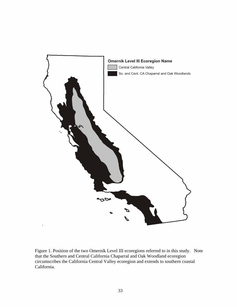
. Figure 1. Position of the two Omernik Level III ecoregions referred to in this study. Note that the Southern and Central California Chaparral and Oak Woodland ecoregion circumscribes the California Central Valley ecoregion and extends to southern coastal California.

33

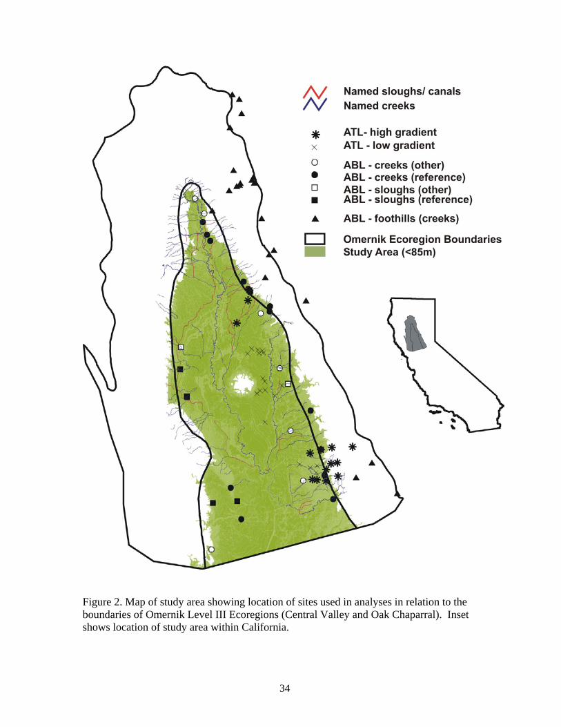
Figure 2. Map of study area showing location of sites used in analyses in relation to the boundaries of Omernik Level III Ecoregions (Central Valley and Oak Chaparral). Inset shows location of study area within California.

34

Figure 3. Watershed boundaries of creeks and sloughs sampled for this study. Note that lower boundaries were approximated based on natural channel positions. Site codes are defined in Appendix D.

35

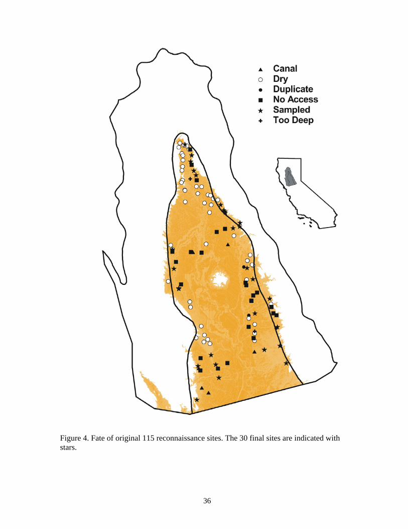
Figure 4. Fate of original 115 reconnaissance sites. The 30 final sites are indicated with stars.

36

Figure 5. Schematic representation of GIS coverages of pesticide application and landcover used in this study.

37

Figure 6. Boxplots of metric scores for ABL creeks and sloughs at Level I taxonomic effort. Asterisks indictate significant differences between creeks and sloughs.

38

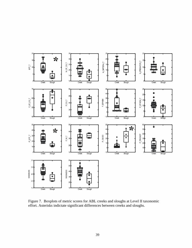
Figure 7. Boxplots of metric scores for ABL creeks and sloughs at Level II taxonomic effort. Asterisks indictate significant differences between creeks and sloughs.

39

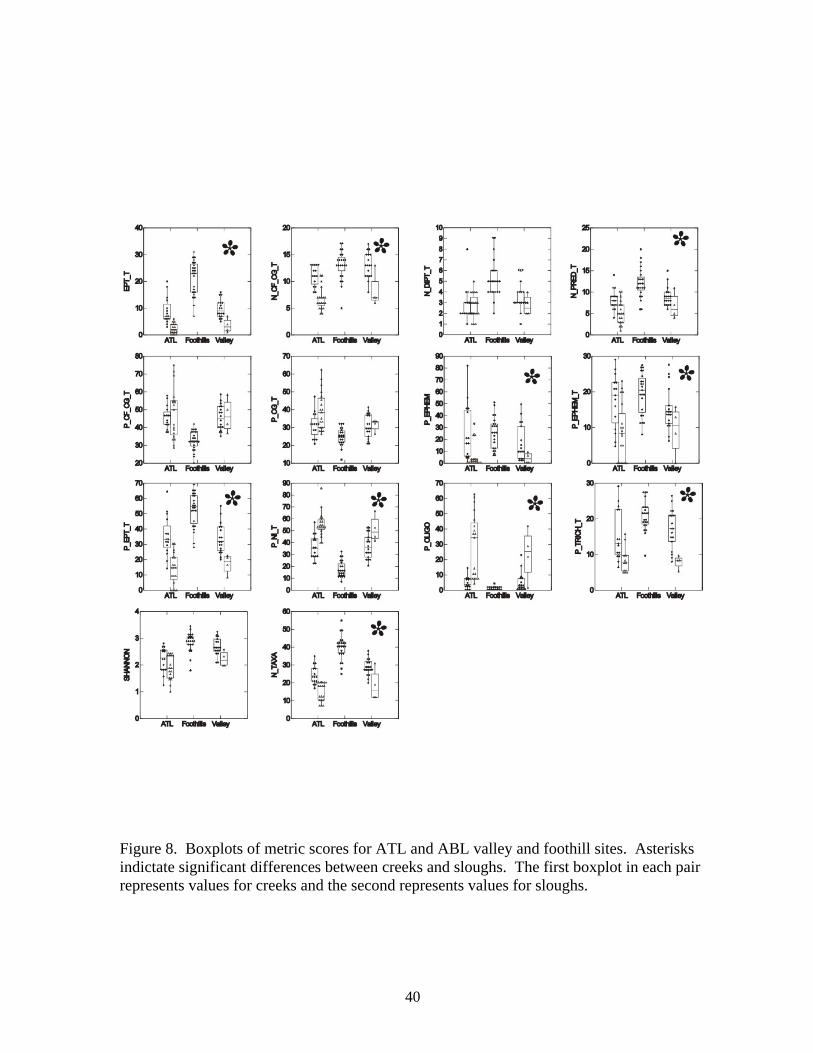
Figure 8. Boxplots of metric scores for ATL and ABL valley and foothill sites. Asterisks indictate significant differences between creeks and sloughs. The first boxplot in each pair represents values for creeks and the second represents values for sloughs.

40

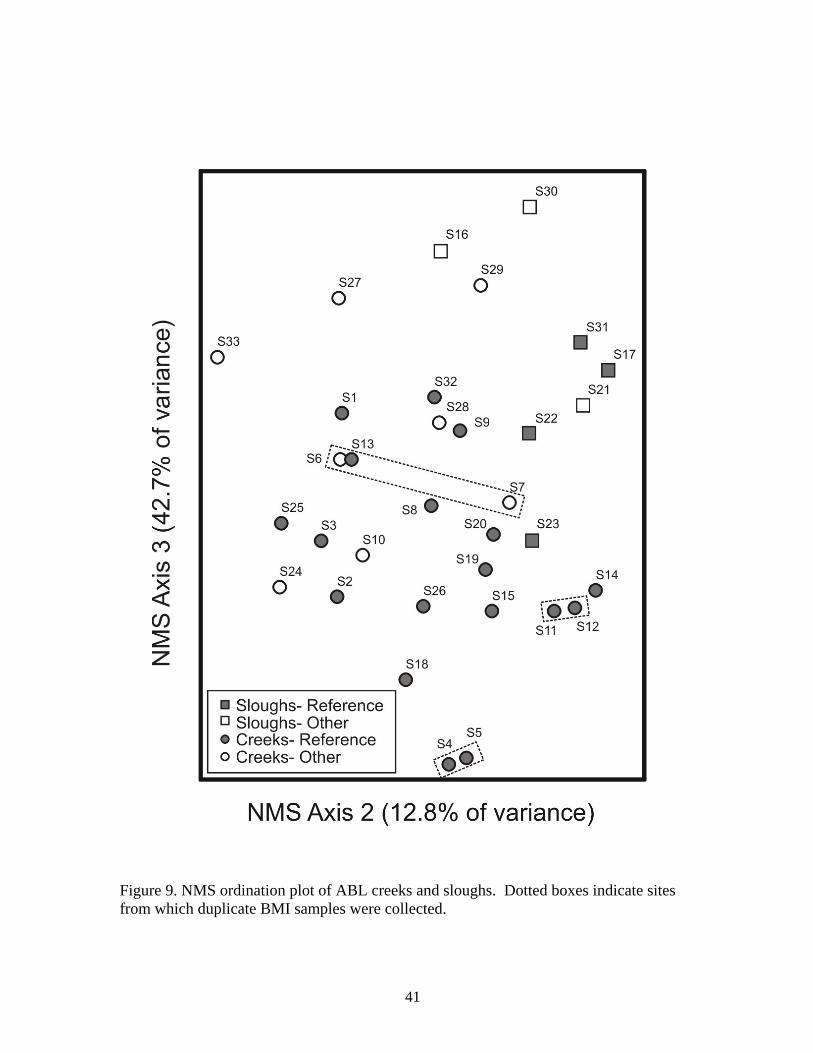
Figure 9. NMS ordination plot of ABL creeks and sloughs. Dotted boxes indicate sites from which duplicate BMI samples were collected.

41

Figure 10. NMS ordination plot of species data for creeks, sloughs and foothills sites. Dotted boxes indicate sites from which duplicate BMI samples were collected.

42

Figure 11. NMS ordination plot of 36 metrics for all analysis datasets. Ellipse overlays describe the approximate boundaries of each group except the ABL non-reference sites.

43

APPENDIX A

Results of field reconnaissance of 115 sites in the Sacramento Valley, including visual assessment and qualitative GIS scores,

initial sampling priority, and final site status

44

APPENDIX B

Field reconnaissance and visual site assessment worksheet

45

APPENDIX C

Thirty two measurements of physical habitat for ABL Sacramento Valley sites, including GIS and visual landuse, substrate characteristics, overall visual

assessment, RBP scores, riparian condition measures, and ambient water chemistry (note that percentages are recorded as proportions in this table)

46

APPENIDX D

Quantitative GIS and physical habitat scores with final reference site selection decisions and comments

47

APPENDIX E

Photographs and Full Site Descriptions for ABL Sacramento Valley Sites

48

APPENDIX F

List of benthic macroinvertebrate taxa identified from samples collected from 30 Central Valley sites with identifications at Level I taxonomy

49

APPENDIX G

List of benthic macroinvertebrate taxa identified from samples collected from 30 Central Valley sites with identifications at Level I taxonomy

50

APPENDIX H

Benthic macroinvertebrate metrics calculated for ABL Sacramento Valley sites at Level I taxonomy (note that percentages are recorded as proportions in this table)

51

APPENDIX I

Benthic macroinvertebrate metrics calculated for ABL Sacramento Valley sites at Level II taxonomy (note that percentages are recorded as proportions in this table)

52

APPENDIX J

Benthic macroinvertebrate metrics calculated for ATL sites at Level I taxonomy

(note that percentages are recorded as proportions in this table)

53

APPENDIX K

Benthic macroinvertebrate metrics calculated for Sierra Foothill sites at Level I taxonomy

(note that percentages are recorded as proportions in this table)

54