ad - sigmobile fading. ho w ev ... ad ho c optimization metrics. the ap osteriori approac h, on the...
TRANSCRIPT
ADAPTIVE EQUALIZATION AND RECEIVER
DIVERSITY FOR INDOOR WIRELESS DATA
COMMUNICATIONS
a dissertation
submitted to the department of electrical engineering
and the committee on graduate studies
of stanford university
in partial fulfillment of the requirements
for the degree of
doctor of philosophy
By
Yumin Lee
August 1997

c Copyright 1997 by Yumin Lee
All Rights Reserved
ii

I certify that I have read this dissertation and that in
my opinion it is fully adequate, in scope and quality, as
a dissertation for the degree of Doctor of Philosophy.
Donald C. Cox(Principal Advisor)
I certify that I have read this dissertation and that in
my opinion it is fully adequate, in scope and quality, as
a dissertation for the degree of Doctor of Philosophy.
John M. Cio�
I certify that I have read this dissertation and that in
my opinion it is fully adequate, in scope and quality, as
a dissertation for the degree of Doctor of Philosophy.
Teresa H. Meng
Approved for the University Committee on Graduate
Studies:
iii

Abstract
Multipath propagation is one of the most challenging problems encountered in a
wireless data communication link. It causes signal fading, delay spread, and Doppler
spread, and can greatly impair the performance of a data communication system.
Multipath mitigation techniques such as adaptive decision-feedback equalization (DFE)
and receiver diversity are thus required for low-error-rate, high-speed wireless data
communications. This dissertation examines these techniques for indoor wireless data
communications. Receiver diversity is known to be an e�ective way of coping with
signal fading. However, indoor wireless radio channels exhibit frequency-selective fad-
ing which introduces inter-symbol interference (ISI), therefore receiver diversity alone
cannot yield satisfactory performance, and more sophisticated signal processing tech-
niques are often required. Adaptive equalization, on the other hand, is known to be
an e�ective measure against ISI. However, adaptive equalization alone cannot miti-
gate the e�ect of signal fading. Integration of diversity and adaptive equalization is
therefore desirable for communication systems such as indoor wireless data networks
which operate in a delay-spread multipath fading environment.
In this dissertation, the e�ects of multipath propagation and their impact on a data
communication system are �rst discussed. A exible baseband model is developed
for indoor wireless communication channels. The adaptive DFE is then treated alone
as an approach for mitigating the e�ect of delay spread. Algorithms for updating
the DFE �lter coe�cients are discussed. These algorithms are classi�ed as channel-
estimation-based adaptation (CEBA) and direct-adaptation (DA). While they have
been compared previously in the literature, in this dissertation new results regarding
their relative performance are obtained using computer simulations that are realistic
iv
for wireless communications. Furthermore, an improved training method referred
to as \synthetic training" is developed and shown to be very e�ective in improving
the performance of the DA DFE. A numerical technique known as \regularization" is
also applied to improve the performance of the channel-estimation-based fractionally-
spaced DFE.
Sampling instant and decision delay optimization, which are crucial to the per-
formance of the adaptive DFE, are also investigated for the adaptive DFE. In this
dissertation, the sampling instant is obtained via a two-step approach from the over-
samples of the received signal. The decision delay is next optimized using the a
priori approach or the a posteriori approach. The a priori approach is evaluated us-
ing previously proposed as well as new, ad hoc optimization metrics. The a posteriori
approach, on the other hand, is �rst demonstrated using an \ideal" technique which
is not realizable. A realizable a posteriori optimization technique, referred to as the
multiple decision delay DFE (MDDDFE), is later developed, and shown to achieve a
performance that is very close to the ideal technique.
Paralleling the discussion on the adaptive DFE, receiver diversity is also presented
alone as a mitigation technique against signal fading. Computer simulation is used
to show that, when used alone, receiver diversity can also signi�cantly improve the
performance of a wireless data communication system. The performance improve-
ments achieved by receiver diversity and adaptive DFE are, however, due to di�erent
reasons. It is therefore very desirable to integrate these two techniques.
The integration of combining and selection diversity with the adaptive DFE is dis-
cussed in detail in this dissertation. The maximal ratio combining DFE (MRCDFE)
is a technique for introducing combining diversity into adaptive DFE, while the se-
lection diversity DFE (SDDFE) is a technique for incorporating selection diversity
into adaptive DFE. For the MRCDFE, the branch DFE �lter coe�cients are jointly
optimized using extensions of the CEBA and DA algorithms. Regularization can also
be applied to improve the performance of the fractionally-spaced MRCDFE. While
the MRCDFE is not new, we obtained new results regarding the relative performance
of the CEBA and DA MRCDFE's, which are consistent with the results we presented
for the single-branch case. For the SDDFE, we developed a new selection rule which
v
is referred to as the maximum a posteriori probability (MAP) selection rule. This
rule is proved to be optimal, in the MAP sense, for a SDDFE. Based on the MAP
selection rule, two new selection metrics are derived and evaluated. Simulation results
show that both the MRCDFE and MAP SDDFE greatly outperform the unequalized
diversity receiver and adaptive DFE without receiver diversity. Furthermore, the new
MAP selection metrics signi�cantly outperform conventional metrics for the SDDFE,
and achieve a performance that is only slightly inferior to the MRCDFE. Since the
branch DFE �lter coe�cients are independently optimized for the SDDFE, it is com-
putationally simpler than the MRCDFE. Adaptive MAP SDDFE is, therefore, an
attractive approach for simultaneously mitigating the impact of signal fading, delay
spread, and small amount of Doppler spread.
vi

Acknowledgments
First and foremost, I thank my advisor, Professor Donald Clyde Cox.
My �rst encounter with Professor Cox was in the Autumn Quarter of 1993, when
I requested to join his research group and was told to try again the next quarter.
When I did, I was again told to wait until the Qualifying Exams (the \Quals") are
over. It was not until after the Quals was I admitted into his research group.
Looking back, joining the \Cox Group" is the best thing that has happened to
me in Stanford University. During the past four years I have acquired from Professor
Cox a great deal of technical knowledge, and a rigorous yet practical attitude towards
research. Furthermore, I have learned from him that many problems cannot be solved
without clearly specifying the assumptions and conditions, therefore \it depends" is
often the best answer to many questions. Working with Professor Cox is indeed a
highly enjoyable, inspiring, and rewarding experience. I feel very honored to have
the chance to work with Professor Cox, and sincerely thank him for his guidance and
support throughout my Ph.D. studies at Stanford University.
I am also deeply indebted to the other members of my orals and reading commit-
tees: Professors John M. Cio�, C. Robert Helms, Teresa H. Meng, and Madihally J.
Narasimha. They scrutinized my research results, made sure that there are no mis-
takes, and gave me many valuable comments. Without them this dissertation would
never have materialized.
I also owe my sincerest gratitude to Dr. David E. Borth of Motorola Incorpo-
rated at Schaumburg, Illinois, and to Paci�c Bell at San Ramon, California, for their
generous support over the course of this research. In the past four years Motorola
has provided for my tuition and stipend. Furthermore, Dr. Borth has taken time to
vii

review every progress report and publication that resulted from this research. Paci�c
Bell, on the other hand, has donated computer equipments which were extensively
used to produce simulation results for this dissertation.
This acknowledgment would not be complete without mentioning the former and
current members of my research group: Bora Akyol, Sung Chun, Hideaki Haruyama,
Kerstin Johnsson, Byoung-Jo Kim, Dae-Young Kim, Matthew Kolz, Persefoni Kyritsi,
Derek Lam, Andy Lee, Angel Lozano, Ravi Narasimhan, Tim Schmidl, Mehdi Soltan,
Je� Stribling, Qinfang Sun, Karen Tian, Bill Wong, and Daniel Wong. I have greatly
enjoyed and bene�ted from our stimulating discussions and interactions. I will always
remember the bitter-sweet memories that we share { especially the two hard-disk
crashes and two computer break-in incidents. I certainly am very fortunate to have
the opportunity to know and work with all of you. Now that some of us are graduating
and some are still working towards the Ph.D. degree, I wish you best of luck in your
careers and studies. I am sure our paths will cross again in the future. I am also
sincerely grateful to our former and current assistants { Jenny Beltran, Lily Huan,
and Marli Williams, for their most helpful administrative support.
During my Ph.D. studies, many friends in Stanford University have helped me
in course work and preparation for the Quals. They are Navin Chaddha, Jonathan
Chang, Kenneth Chang, Jiunn-Tsair Chen, Pei-chun Chiang, Jimmy Chuang, Suhas
Diggavi, Min-Chen Ho, Winston Lee, Jenwei Liang, Chun-Yi Liao, Janray Liao, Ming-
Chang Liu, Chung-Li Lu, Hui-Ling Lu, Zartash Uzmi, Yao-Ting Wang, Clive Wu,
Tien-Chun Yang, and many others. Thanks to them I have cleared many hurdles to
reach the present stage.
In closing I would like to mention some of my oldest and best friends: Yea-Hueay
Chang of Northwestern University, Ju-Hsien Kao and Hsing-Chuan Su of Stanford
University, and Hao-Hsuan Chiu of Syracuse University. Yea-Hueay is, and always will
be, a very special part of my life. Ju-Hsien is from a completely di�erent background
{ mechanical engineering, yet he sat through my oral defense without falling asleep.
Hao-Hsuan is a very good sounding board and travel companion. Thank you for your
love, support, encouragement, and friendship.
I dedicate this dissertation to my parents and brother.
viii
Contents
Abstract iv
Acknowledgments vii
1 Introduction 1
1.1 Dissertation Outline . . . . . . . . . . . . . . . . . . . . . . . . . . . 3
1.2 Contributions . . . . . . . . . . . . . . . . . . . . . . . . . . . . . . . 4
2 Multipath Propagation 6
2.1 Signal Fading . . . . . . . . . . . . . . . . . . . . . . . . . . . . . . . 8
2.2 Delay Spread . . . . . . . . . . . . . . . . . . . . . . . . . . . . . . . 10
2.3 Doppler Spread . . . . . . . . . . . . . . . . . . . . . . . . . . . . . . 14
2.4 Baseband Indoor Wireless Channel Model . . . . . . . . . . . . . . . 17
2.4.1 Simulated Power-Delay Pro�le . . . . . . . . . . . . . . . . . . 20
2.4.2 Simulated Doppler Spectrum . . . . . . . . . . . . . . . . . . . 20
2.5 Summary . . . . . . . . . . . . . . . . . . . . . . . . . . . . . . . . . 23
3 Adaptive Decision-Feedback Equalization 24
3.1 System Model . . . . . . . . . . . . . . . . . . . . . . . . . . . . . . . 24
3.2 Inter-Symbol Interference . . . . . . . . . . . . . . . . . . . . . . . . . 26
3.3 Adaptive DFE . . . . . . . . . . . . . . . . . . . . . . . . . . . . . . . 31
3.3.1 Channel Estimation Based Adaptation . . . . . . . . . . . . . 33
3.3.2 Direct Adaptation . . . . . . . . . . . . . . . . . . . . . . . . 37
3.4 Simulation Results . . . . . . . . . . . . . . . . . . . . . . . . . . . . 40
ix

3.4.1 Synthetic Training for DA DFE . . . . . . . . . . . . . . . . . 41
3.4.2 Comparison of CEBA and DA DFE . . . . . . . . . . . . . . . 46
3.5 CEBA DFE with Regularization . . . . . . . . . . . . . . . . . . . . . 49
3.6 Summary . . . . . . . . . . . . . . . . . . . . . . . . . . . . . . . . . 52
4 DFE Timing Alignment 54
4.1 Sampling Instant Optimization . . . . . . . . . . . . . . . . . . . . . 55
4.2 Decision-Delay Optimization . . . . . . . . . . . . . . . . . . . . . . . 58
4.2.1 A Priori Optimization . . . . . . . . . . . . . . . . . . . . . . 58
4.2.2 A Posteriori Optimization . . . . . . . . . . . . . . . . . . . . 60
4.3 Simulation Results . . . . . . . . . . . . . . . . . . . . . . . . . . . . 60
4.3.1 Sampling Instant Optimization . . . . . . . . . . . . . . . . . 61
4.3.2 Decision Delay Optimization . . . . . . . . . . . . . . . . . . . 64
4.4 Summary . . . . . . . . . . . . . . . . . . . . . . . . . . . . . . . . . 68
5 Receiver Diversity 71
5.1 Combining Diversity DFE . . . . . . . . . . . . . . . . . . . . . . . . 74
5.1.1 CEBA MRCDFE and Regularization . . . . . . . . . . . . . . 75
5.1.2 DA MRCDFE with Synthetic Training . . . . . . . . . . . . . 80
5.2 Simulation Results . . . . . . . . . . . . . . . . . . . . . . . . . . . . 80
5.3 Summary . . . . . . . . . . . . . . . . . . . . . . . . . . . . . . . . . 85
6 MAP Selection Diversity DFE 88
6.1 Selection Diversity DFE . . . . . . . . . . . . . . . . . . . . . . . . . 92
6.2 MAP Selection Metric for SDDFE . . . . . . . . . . . . . . . . . . . . 93
6.3 Computation of Selection Metric . . . . . . . . . . . . . . . . . . . . . 96
6.4 Simulation Results . . . . . . . . . . . . . . . . . . . . . . . . . . . . 98
6.5 Summary . . . . . . . . . . . . . . . . . . . . . . . . . . . . . . . . . 105
7 Multiple Decision Delay DFE 107
7.1 Multiple Decision Delay DFE . . . . . . . . . . . . . . . . . . . . . . 109
7.2 The DFE Controller . . . . . . . . . . . . . . . . . . . . . . . . . . . 110
x
7.3 Simulation Results . . . . . . . . . . . . . . . . . . . . . . . . . . . . 112
7.4 Summary . . . . . . . . . . . . . . . . . . . . . . . . . . . . . . . . . 116
8 Conclusions 118
8.1 Dissertation Summary . . . . . . . . . . . . . . . . . . . . . . . . . . 118
8.2 Future Work . . . . . . . . . . . . . . . . . . . . . . . . . . . . . . . . 124
A Baseband Equivalent Power-Delay Pro�le 126
B Baseband Equivalent Doppler Spectrum 128
C The Least-Squares Lattice DFE 130
D Optimality of MAP Selection Rule 136
Bibliography 138
xi

List of Tables
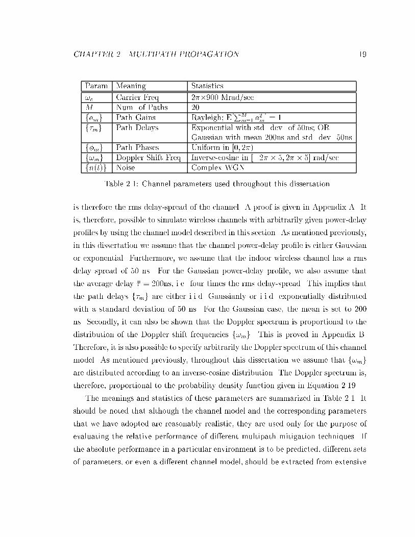
2.1 Channel parameters used throughout this dissertation. . . . . . . . . 19
7.1 Average complexity of one- and two-branch MDDDFE using SERDFE
for d = 0:5 and average SNR of 10, 15 and 20 dB. The average com-
plexity without pruning is also shown. The channel has a Gaussian
power-delay pro�le with a rms delay spread of 50 ns and average delay
of 200 ns. . . . . . . . . . . . . . . . . . . . . . . . . . . . . . . . . . 115
C.1 The dimensionalities of the variables in the LSL DFE algorithm. . . . 135
xii

List of Figures
2.1 Multipath propagation in indoor environments. The signal transmitted
by the transmitter (T) is attenuated and re ected by the walls and
oors. As a consequence the receiver (R) receives multiple distorted
copies of the transmitted signal. . . . . . . . . . . . . . . . . . . . . . 7
2.2 Normalized plots of the Ricean distribution. The numbers labeled on
the curve denote values of �pP. � = 0 corresponds to the Rayleigh
distribution. . . . . . . . . . . . . . . . . . . . . . . . . . . . . . . . . 11
2.3 (a) Normalized exponential power-delay pro�le. (b) Normalized Gaus-
sian power-delay pro�le. �� = 4S in this plot. . . . . . . . . . . . . . . 13
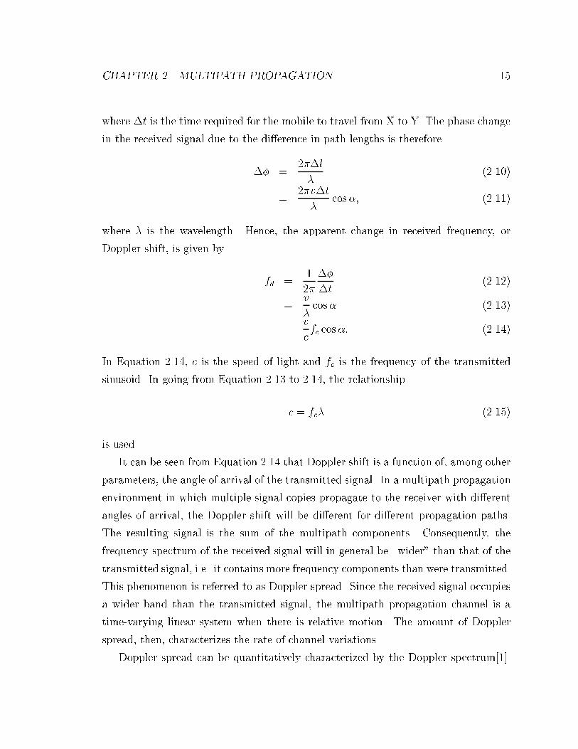
2.4 Illustration of Doppler shift in the free-space propagation environment.
The receiver moves at a constant velocity v along a direction that forms
an angle � with the incident wave. . . . . . . . . . . . . . . . . . . . 14
2.5 The Doppler spectrum corresponding to uniformly distributed angles
of arrival (see Equation 2.16). . . . . . . . . . . . . . . . . . . . . . . 16
2.6 Simulated power-delay pro�les obtained from 200 replications. (a) The
path delays are exponentially distributed with a standard deviation of
50 ns. (b) The path delays are Gaussianly distributed with a mean of
200 ns and standard deviation of 50 ns. . . . . . . . . . . . . . . . . . 21
2.7 Simulated Doppler spectrum obtained from 200 replications. The Doppler
shift frequencies are generated according to Table 2.1 . . . . . . . . . 22
3.1 Baseband model of a wireless data communication system. . . . . . . 25
xiii
3.2 Examples of jp(t)j. (a) When the channel delay-spread is insigni�cant,
very little ISI is introduced. (b) When the channel delay-spread is
signi�cant, the ISI is severe. . . . . . . . . . . . . . . . . . . . . . . . 30
3.3 Block diagram of an adaptive decision-feedback equalizer. . . . . . . . 31
3.4 The channel-estimation-based adaptation DFE. . . . . . . . . . . . . 37
3.5 Prepending the STS to the received waveform for synthetic training
for the DA DFE. . . . . . . . . . . . . . . . . . . . . . . . . . . . . . 40
3.6 The average BER of the symbol-spaced (K = 1) DA DFE with syn-
thetic training. The channel is assumed to have a Gaussian power-delay
pro�le with a rms delay-spread of 50 ns and average delay of 200 ns.
The average SNR is 15 dB. Di�erent training sequence lengths Q and
STS lengths Qs are used. . . . . . . . . . . . . . . . . . . . . . . . . . 42
3.7 Average BER of the symbol-spaced (K = 1) DA DFE using various
CPR estimate lengths for synthetic training. �1 and �2 are both set
to be equal to the value of the abscissa. The channel has a Gaussian
power-delay pro�le with a normalized delay-spread of 0.5. The rms
delay-spread and average delay are 50 ns and 200 ns, respectively. The
average SNR is 15 dB. Synthetic training with Q = Qs = 15 is used. . 44
3.8 The average BER of the half-symbol-spaced (K = 2) DA DFE with
synthetic training. The channel is assumed to have a Gaussian power-
delay pro�le with a rms delay-spread of 50 ns and average delay of 200
ns. The average SNR is 15 dB. Di�erent training sequence lengths Q
and STS lengths Qs are used. . . . . . . . . . . . . . . . . . . . . . . 44
3.9 Average BER of the half-symbol-spaced (K = 2) DA DFE using vari-
ous CPR estimate lengths for synthetic training. �1 and �2 are both set
to be equal to the value of the abscissa. The channel has a Gaussian
power-delay pro�le with a normalized delay-spread of 0.5. The rms
delay-spread and average delay are 50 ns and 200 ns, respectively. The
average SNR is 15 dB. Synthetic training with Q = Qs = 15 is used. . 45
xiv
3.10 Average BER of CEBA and DA DFE's: (a) as a function of average
SNR at d = 0:5; (b) as a function of d at 15dB average SNR. The
channel is assumed to have a Gaussian power-delay pro�le with a rms
delay-spread of 50 ns and average delay of 200 ns. . . . . . . . . . . 47
3.11 Average BER of the half-symbol-spaced (K = 2) CEBA DFE with
regularization: (a) as a function of average SNR at d = 0:5; (b) as a
function of d at 15dB average SNR. The average BER's CEBA without
regularization and DA with K = 2 are also shown. The channel is
assumed to have a Gaussian power-delay pro�le with a rms delay-
spread of 50 ns and average delay of 200 ns. . . . . . . . . . . . . . . 51
4.1 Block diagram of an adaptive decision-feedback equalizer. . . . . . . . 54
4.2 The average BER of the symbol-spaced DA DFE using di�erent sam-
pling instant optimization techniques. The channel has a Gaussian
power-delay pro�le with a rms delay-spread of 50 ns and average delay
of 200 ns. The average SNR is 15 dB. . . . . . . . . . . . . . . . . . . 62
4.3 The average BER of the half-symbol-spaced DA DFE using di�erent
sampling instant optimization techniques. The channel has a Gaussian
power-delay pro�le with a rms delay-spread of 50 ns and average delay-
spread of 200 ns. The average SNR is 15 dB. . . . . . . . . . . . . . . 64
4.4 Average BER as a function of average SNR for di�erent decision delay
optimization schemes, �xed delay and ideal cases. The channel has
a Gaussian power-delay pro�le with normalized delay-spread d = 0:5.
Symbol-spaced DA DFE's are used. . . . . . . . . . . . . . . . . . . . 65
4.5 Average BER as a function of normalized delay-spread for di�erent
decision delay optimization schemes, �xed delay and ideal cases. The
channel has a Gaussian power-delay pro�le with an average SNR of 15
dB. Symbol-spaced DA DFE's are used. . . . . . . . . . . . . . . . . 66
xv
4.6 Average BER as a function of average SNR for di�erent decision delay
optimization schemes, �xed delay and ideal cases. The channel has
a Gaussian power-delay pro�le with normalized delay-spread d = 0:5.
Half-symbol-spaced DA DFE's are used. . . . . . . . . . . . . . . . . 67
4.7 Average BER as a function of normalized delay-spread for di�erent
decision delay optimization schemes, �xed delay and ideal cases. The
channel has a Gaussian power-delay pro�le with an average SNR of 15
dB. Half-symbol-spaced DA DFE's are used. . . . . . . . . . . . . . 68
5.1 Block diagram for selection diversity. One diversity branch is selected
according to some selection rule. . . . . . . . . . . . . . . . . . . . . 73
5.2 Block diagram for combining diversity. The received signals are am-
pli�ed, co-phased and summed. . . . . . . . . . . . . . . . . . . . . . 74
5.3 The maximal-ratio combining DFE. . . . . . . . . . . . . . . . . . . . 75
5.4 Average BER's of the unequalized diversity combiner (DIV-ONLY),
half-symbol-spaced DA DFE without diversity (DFE-ONLY), and dual
diversity (L = 2) DA and CEBA MRCDFE's: (a) as functions of
average SNR at d = 0:5; and (b) as functions of d at 15dB average
SNR. The channel has a Gaussian power-delay pro�le with a rms delay-
spread of 50 ns and average delay of 200 ns. . . . . . . . . . . . . . . 82
5.5 Average BER's of the half-symbol-spaced DA DFE without diversity
(DFE-ONLY), dual diversity (L = 2) DAMRCDFE, and dual diversity
(L = 2) CEBA MRCDFE with regularization: (a) as functions of
average SNR at d = 0:5; and (b) as functions of d at 15dB average
SNR. The channel has a Gaussian power-delay pro�le with a rms delay-
spread of 50 ns and average delay of 200 ns. . . . . . . . . . . . . . . 86
6.1 Possible structures for the selection diversity DFE: (a) Selection is done
before equalization; (b) Selection is done after equalization. . . . . . . 89
6.2 Possible selection schemes for the SDDFE. . . . . . . . . . . . . . . . 90
6.3 Selection-diversity decision-feedback equalizer. . . . . . . . . . . . . . 90
xvi
6.4 Average BER's of the various selection metrics as functions of the
average SNR. The channel has an exponential power-delay pro�le with
a rms delay-spread of 50 ns. The normalized delay spread d is 0.5. As
noted in the text, the IDEAL case is not realizable. . . . . . . . . . . 100
6.5 Conditional probability of correct branch selection given that exactly
one diversity branch decision is wrong. The channel has an exponential
power-delay pro�le with a rms delay-spread of 50 ns. The normalized
delay-spread d is 0.5. . . . . . . . . . . . . . . . . . . . . . . . . . . . 102
6.6 Average BER's as functions of the normalized delay-spread d. The
channel has an exponential power-delay pro�le with 50 ns rms delay-
spread. The average SNR is 15 dB. The IDEAL case is not realizable
as noted in the text. . . . . . . . . . . . . . . . . . . . . . . . . . . . 103
6.7 Average BER's of the various selection metrics as functions of the
average SNR. The channel has a Gaussian power-delay pro�le with a
rms delay-spread of 50 ns and average delay of 200 ns. The normalized
delay spread d is set to 0.5. The IDEAL case is not realizable as noted
in the text. . . . . . . . . . . . . . . . . . . . . . . . . . . . . . . . . 104
6.8 Average BER's as functions of the normalized delay-spread d. The
channel has a Gaussian power-delay pro�le with a rms delay-spread of
50 ns and average delay of 200 ns. The average SNR is 15 dB. The
IDEAL case is not realizable as noted in the text. . . . . . . . . . . . 105
7.1 Structure of the MDDDFE. . . . . . . . . . . . . . . . . . . . . . . . 109
7.2 Algorithm for pruning redundant DFE's. This algorithm is repeated
once every R symbols. . . . . . . . . . . . . . . . . . . . . . . . . . . 111
7.3 Average BER as a function of average SNR at d = 0:5 for the MD-
DDFE, �xed decision delay, and ideal cases. Half-symbol-spaced DA
MDDDFE's used here. The channel has a Gaussian power-delay pro�le
with a rms delay-spread of 50ns and average delay of 200 ns. . . . . . 114
xvii

7.4 Average BER as a function of normalized delay-spread at average SNR
of 15dB for the MDDDFE, �xed decision delay and ideal cases. Half-
symbol-spaced DA MDDDFE's used here. The channel has a Gaussian
power-delay pro�le with a rms delay-spread of 50ns and average delay
of 200 ns. . . . . . . . . . . . . . . . . . . . . . . . . . . . . . . . . . 115
C.1 (a) The block diagram of a LSL DFE. Matrix weights are not explicitly
shown. The block labeled \D" denotes a unit-sample delay; (b) The
block diagram of a LSL stage. Matrix weights are not explicitly shown.
The block labeled \D" denotes a unit-sample delay. . . . . . . . . . . 131
xviii
Chapter 1
Introduction
With recent advances in communications, signal processing, and computer technolo-
gies, the dream of wireless networking for data communication systems has become an
achievable goal. One attractive application of wireless networking is the indoor wire-
less local area network (WLAN). First, since it allows for mobility of users, re-wiring
is unnecessary when a user of a WLAN moves. This can be especially important for
users of portable data terminals. Secondly, since the WLAN operates in indoor en-
vironments, high-speed data transmission is possible without requiring an unrealistic
amount of transmitter power. This is an important aspect for many data applications.
One of the most important building blocks for an indoor WLAN is the wireless
data communication link. For a WLAN to function properly, reliable wireless data
communication links must �rst be established. Multipath propagation is one of the
most challenging problems encountered in a wireless data communication link. In a
multipath propagation environment, the transmitted electro-magnetic signal propa-
gates to the receiver via many di�erent paths. In general, these propagation paths
have di�erent amplitude gains, phase shifts, angles of arrival, and path delays that
are functions of the re ection structure of the environment. The e�ects of multipath
propagation include signal fading, delay spread, and, when there is relative motion
between the transmitter and receiver, Doppler spread. Signal fading refers to the phe-
nomenon that in a multipath propagation environment, the received signal strength
is strongly dependent on the locations of the transmitter and receiver. This is caused
1
CHAPTER 1. INTRODUCTION 2
by the interference between signals propagating through di�erent paths. Delay spread
refers to the spread of the duration of the received signal with respect to the trans-
mitted signal. This is due to the di�erent delays associated with the propagation
paths. Delay spread introduces inter-symbol interference (ISI) in a digital wireless
communication system, which limits the achievable transmission rate. It also causes
di�culties for symbol-timing recovery in a digital demodulator. Doppler spread, on
the other hand, refers to the spread of the frequency spectrum of the received signal
with respect to that of the transmitted signal, when there is relative motion between
the transmitter and the receiver. This is due to the di�erent angles of arrival associ-
ated with the propagation paths. Since the spectrum of the received signal is wider
in frequency than that of the transmitted signal, the multipath propagation channel
is clearly a time-varying system. Adaptive signal processing techniques are there-
fore required to track channel variations for a mobile digital wireless communication
system operating in a multipath propagation environment.
This dissertation discusses the digital signal processing techniques that can be
used to mitigate the impact of multipath propagation on the performance of a point-
to-point single-user indoor high-speed wireless data communication link. Adaptive
decision-feedback equalization is a solution for mitigating delay spread and Doppler
spread. In this technique, adaptive linear discrete-time �nite impulse response (FIR)
�lters are used to process the received signal. The FIR �lters can be optimized directly
using the received signal samples, or indirectly through channel estimation. Since the
adaptive equalizer operates in discrete-time, the sampling instants must be deter-
mined before equalization starts. Furthermore, since FIR �lters are used, a design
parameter referred to as the \decision delay" must also be determined. The optimiza-
tion of the sampling instants and decision delay is referred to as \timing alignment" in
this dissertation. This dissertation compares the performance of di�erent adaptation
techniques using realistic computer simulation, and also investigates di�erent timing
alignment approaches for adaptive decision-feedback equalizers (DFE's).
Receiver diversity, which makes use of multiple receiver antennas, is a technique
used to combat signal fading. If the receiver antennas are spaced far enough apart (on
the order of a half-wavelength), the wireless channels corresponding to these antennas
CHAPTER 1. INTRODUCTION 3
will be approximately uncorrelated. In this case it is unlikely for both antennas to si-
multaneously experience a deep signal fade. The received signals at the output of the
branch antennas can therefore be combined either by taking their weighted average
(combining diversity) or by simply choosing the \best" (selection diversity). Receiver
diversity has been shown to be very e�ective against fading. However, it alone is not
very e�ective in coping with delay spread, and ways to incorporate adaptive equal-
ization into receiver diversity are highly desirable. This dissertation discusses novel
approaches for introducing diversity into the adaptive DFE in order to simultane-
ously mitigate the three di�culties caused by multipath propagation. In particular,
an optimal selection diversity scheme is derived for adaptive DFE's. Simulation re-
sults show that the new scheme discussed in this dissertation can indeed outperform
conventional selection diversity schemes.
1.1 Dissertation Outline
Chapter 2 of this dissertation discusses multipath propagation. Small-scale e�ects of
multipath propagation are brie y described, and a simple baseband model is devel-
oped for use in subsequent chapters.
The adaptive DFE is discussed in Chapter 3. The DFE can be optimized directly
from the received signal samples, or indirectly through channel estimation. These
two approaches have been compared by previous researchers under certain assump-
tions that are not applicable to wireless data communication links. In this chapter,
we compare the performance of these two approaches using realistic computer simu-
lation over a broad range of wireless channel conditions. Performance enhancement
techniques are also investigated for both approaches.
Chapter 4 provides a treatment of timing alignment for adaptive DFE's. The
timing alignment parameters are de�ned mathematically, and practical approaches
for optimizing these parameters are discussed.
In Chapter 5, the concept of receiver diversity is introduced. It is demonstrated
here that, while diversity alone is very e�ective against fading, it is not very e�ective
in coping with delay-spread. A previously proposed structure to combine receiver

CHAPTER 1. INTRODUCTION 4
diversity and equalization is also described in this chapter. This approach is referred
to as the maximal-ratio combining DFE (MRCDFE), which introduces combining
diversity into a DFE. Computer simulations are used to compare di�erent adaptation
techniques for the MRCDFE.
Chapter 6 describes a novel approach for incorporating adaptive decision-feedback
equalization into selection diversity. This approach, referred to as the maximum a
posteriori probability (MAP) selection diversity, can be shown to be optimal in the
MAP sense for selection-diversity DFE's. Simulation results show that the proposed
approach is very e�cient. It signi�cantly outperforms conventional selection-diversity
DFE's. Furthermore, the MAP selection diversity DFE performs almost as well as,
but is signi�cantly simpler, than the MRCDFE.
In Chapter 7, the selection diversity technique derived in Chapter 6 is applied to
DFE decision delay optimization. An adaptive DFE structure with multiple decision
delays is also proposed and analyzed. Simulation results show that the proposed
structure can greatly improve the performance of a conventional adaptive DFE.
Conclusions are given in Chapter 8.
1.2 Contributions
Chapter 3 reports simulation results for the comparison of the channel-estimation-
based adaptation and direct adaptation DFE's. These results take into account the
randomness of the wireless channel lengths, and thus are more realistic than previous
work in the literature. The synthetic training approach for improving the performance
of an adaptive DFE is also novel. The same analyses are also extended in Chapter 5
to accommodate receiver diversity.
Chapter 4 proposes and evaluates an ad hoc, yet simple, metric for DFE decision
delay optimization. It is also shown here that the a posteriori method for decision
delay optimization can potentially outperform conventional schemes. In the a poste-
riori method, multiple DFE's with di�erent decision delays are used to obtain several
decoded bursts, and the burst containing the fewest errors is chosen as the �nal out-
put. A practically implementable structure, referred to as the multiple decision delay
CHAPTER 1. INTRODUCTION 5
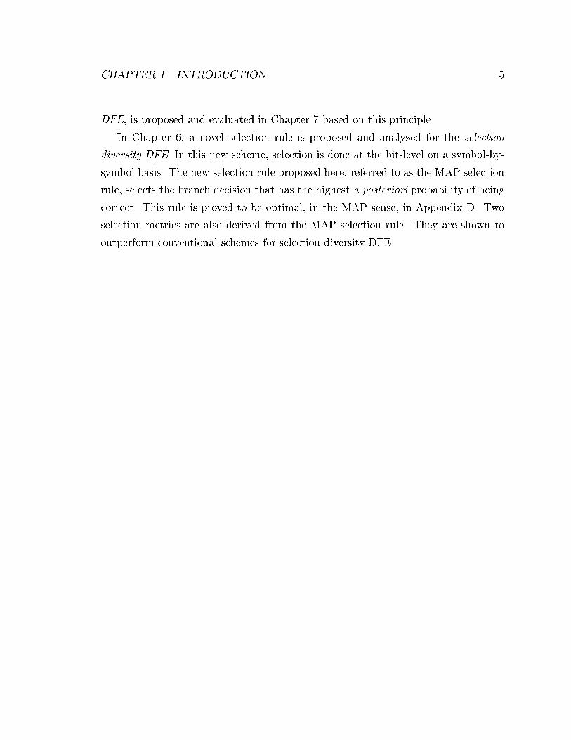
DFE, is proposed and evaluated in Chapter 7 based on this principle.
In Chapter 6, a novel selection rule is proposed and analyzed for the selection
diversity DFE. In this new scheme, selection is done at the bit-level on a symbol-by-
symbol basis. The new selection rule proposed here, referred to as the MAP selection
rule, selects the branch decision that has the highest a posteriori probability of being
correct. This rule is proved to be optimal, in the MAP sense, in Appendix D. Two
selection metrics are also derived from the MAP selection rule. They are shown to
outperform conventional schemes for selection diversity DFE.

Chapter 2
Multipath Propagation
In a wireless communication channel, the transmitted signal generally propagates
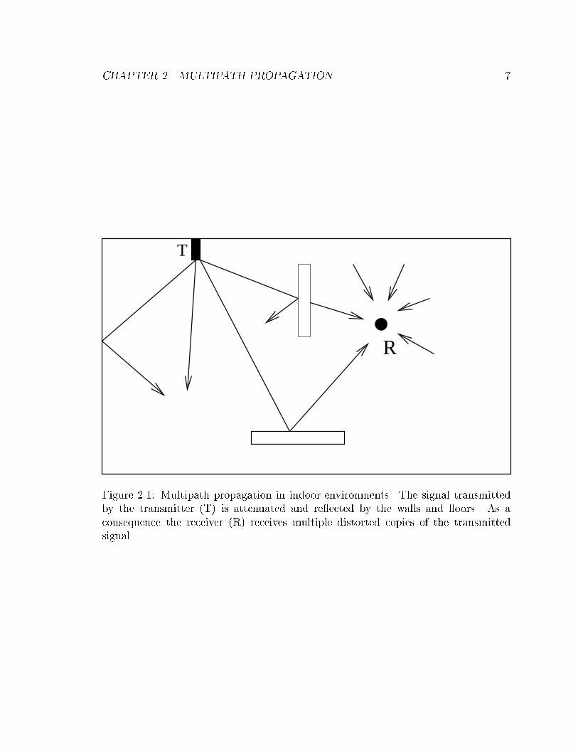
to the receiver antenna through many di�erent paths. This phenomenon, depicted
in Figure 2.1 for indoor environments, is termed multipath propagation. Multipath
propagation is due to the multiple re ections caused by re ectors and scatterers in the
environment. Possible re ectors and scatterers may include mountains, hills and trees
in rural environments, buildings and vehicles in built-up urban environments, or walls
and oors in indoor environments. The receiver antenna will therefore receive multiple
copies of the transmitted signal. Since di�erent versions of the signal propagate
through di�erent paths, they will in general have di�erent attenuation, phase shifts,
time delays and angles of arrival. The receiver antenna output is the sum of the
multiple signal copies weighted by the antenna gain pattern.
Multipath propagation is a complicated phenomenon that is very di�cult to char-
acterize. One common approach is to treat the received signal as a spatial-temporal
random process. The statistics of this random process can be collected from extensive
�eld measurements in selected operation environments. Since the properties of the
received signal are clearly a strong function of the multipath environment, statistical
characterization of the received signal is often done in a two-step process. In the
�rst step, it is assumed that the multipath environment is �xed, and variations of the
received signal are measured for the given multipath environment. The statistics thus
collected are referred to as small-scale variations, because they are usually obtained
6
CHAPTER 2. MULTIPATH PROPAGATION 7
T
R
Figure 2.1: Multipath propagation in indoor environments. The signal transmitted
by the transmitter (T) is attenuated and re ected by the walls and oors. As a
consequence the receiver (R) receives multiple distorted copies of the transmitted
signal.

CHAPTER 2. MULTIPATH PROPAGATION 8
from measurement data obtained at various locations in a small area. In the second
step, variations of the small-scale statistics are determined from measurements taken
in di�erent multipath environments. These variations are referred to as large-scale
variations, because they are obtained from measurement data taken at various loca-
tions in a large area. In this dissertation, we focus on mitigating the e�ects of the
small-scale variations using digital signal processing techniques. These small-scale
variations, including signal fading, delay-spread and Doppler-spread, are discussed in
the remainder of this chapter. For a treatment of large-scale variations, readers are
referred to [1].
2.1 Signal Fading
Signal fading refers to the rapid change in received signal strength over a small travel
distance or time interval. This occurs because in a multipath propagation environ-
ment, the signal received by the mobile at any point in space may consist of a large
number of plane waves having randomly distributed amplitudes, phases, delays and
angles of arrival. These multipath components combine vectorily at the receiver an-
tenna. They may combine constructively or destructively at di�erent points in space,
causing the signal strength to vary with location.
If the objects in a radio channel are stationary, and channel variations are con-
sidered to be only due to the motion of the mobile, then signal fading is a purely
spatial phenomenon. A receiver moving at high speed may traverse through several
fades in a short period of time. If the mobile moves at low speed, or is stationary,
then the receiver may experience a deep fade for an extended period of time. Reliable
communication can then be very di�cult because of the very low signal-to-noise ratio
(SNR) at points of deep fades.
Extensive �eld measurements have previously been done[2, 3, 4, 5] to characterize
the small-scale spatial distribution of the received signal amplitude in multipath prop-
agation environments. It has been found that for many environments, the Rayleigh
distribution provides a good �t to the signal amplitude measurement in environments

CHAPTER 2. MULTIPATH PROPAGATION 9
where no line-of-sight or dominant path exists[2, 5, 6]. The probability density func-
tion of the Rayleigh distribution is given by[7]
f(r) =
8<:
r
Pexp
�� r
2
P
�r � 0:
0 otherwise;(2.1)
where P is the parameter of the distribution. A normalized plot of the Rayleigh
probability density function is shown in Figure 2.2. The Rayleigh distribution is
related to the zero-mean Gaussian distribution in the following manner. Let XI and
XQ be two independent, identically distributed (i.i.d.) zero-mean Gaussian random
variables with variance P. The marginal probability density functions of XI and XQ
are given by
f(x) =1p2�P
exp
� x2
2P
!;�1 < x <1: (2.2)
Then the random variable R, de�ned as
R =qX2
I+X2
Q; (2.3)
is distributed according to the Rayleigh probability density function given in Equa-
tion 2.1. The fact that the Rayleigh distribution provides a good �t to the mea-
sured signal amplitudes in a non-line-of-sight environment can be explained as fol-
lows. When a signal is transmitted through a multipath propagation channel, the
in-phase and quadrature-phase components of the received signal are sums of many
random variables. Because there is no line-of-sight or dominant path, these random
variables are approximately zero-mean. Therefore, by the central limit theorem, the
in-phase and quadrature-phases components can be modeled approximately as zero-
mean Gaussian random processes. The amplitude, then, is approximately Rayleigh
distributed.
On the other hand, when line-of-sight paths exist in a multipath propagation
environment, or when there is a dominant re ected path, the Ricean distribution
is a good statistical characterization of the signal amplitude distribution[4, 5]. The
Ricean distribution is related to the Gaussian distribution in a manner similar to the

CHAPTER 2. MULTIPATH PROPAGATION 10
relationship between the Rayleigh and Gaussian distributions. In particular, let XI
and XQ be independent Gaussian random variables with variance P . Furthermore,
assume that E[XI ] = � and E[XQ] = 0. Then the random variable R, de�ned in
Equation 2.3, is distributed according to the Ricean distribution. Thus, one can see
that when a dominant path exist in a multipath propagation environment, by the
central limit theorem, the signal amplitudes are approximately Ricean distributed
when the number of paths is large. The probability density function of the Ricean
distribution is given by[7]
f(r) =
8<:
r
PI0�r�
P
�exp
�� r
2+�2
2P
�; r � 0;
0 otherwise,(2.4)
where
I0(x) � 1
2�
Z 2�
0exp (x cos �)d� (2.5)
is the zeroth-order modi�ed Bessel function of the �rst kind. Note that there are two
parameters in Equation 2.4. P is the variance of the underlying Gaussian random
variable and � is the amplitude of the line-of-sight or dominant component. Normal-
ized plots of the Ricean distribution with di�erent values of � are shown in Figure 2.2,
in which � = 0 corresponds to the Rayleigh distribution. As � tends to in�nity, the
Ricean distribution converges to a Gaussian distribution.
2.2 Delay Spread
As mentioned previously, in a multipath propagation environment, the received sig-
nal consists of a large number of components having di�erent delays. Consequently,
when a \narrow" pulse is transmitted over a multipath propagation channel, dis-
torted replicas of the transmitted pulse arrive at the receiver at various di�erent
times, making the received signal \wider" in time than the transmitted signal. This
phenomenon is referred to as delay spread. The signi�cance of delay spread depends
on the time-width of the signal relative to that of the channel, hence a quantitative
characterization of the severeness of channel delay-spread is necessary.
CHAPTER 2. MULTIPATH PROPAGATION 11
rP-1/2
f(r)
P1/
2
0 2 4 6 8 10
0.7
0.6
0.5
0.4
0.3
0.2
0.1
0
3.0 5.0
0 (Rayleigh)
1.0
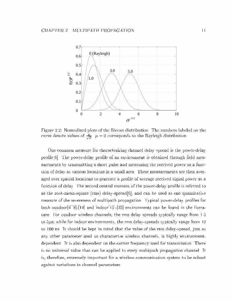
Figure 2.2: Normalized plots of the Ricean distribution. The numbers labeled on the
curve denote values of �pP. � = 0 corresponds to the Rayleigh distribution.
One common measure for characterizing channel delay spread is the power-delay
pro�le[6]. The power-delay pro�le of an environment is obtained through �eld mea-
surements by transmitting a short pulse and measuring the received power as a func-
tion of delay at various locations in a small area. These measurements are then aver-
aged over spatial locations to generate a pro�le of average received signal power as a
function of delay. The second central moment of the power-delay pro�le is referred to
as the root-mean-square (rms) delay-spread[6], and can be used as one quantitative
measure of the severeness of multipath propagation. Typical power-delay pro�les for
both outdoor[4][8]-[14] and indoor[15]-[25] environments can be found in the litera-
ture. For outdoor wireless channels, the rms delay-spreads typically range from 1.5
to 5�s; while for indoor environments, the rms delay-spreads typically range from 10
to 100 ns. It should be kept in mind that the value of the rms delay-spread, just as
any other parameter used to characterize wireless channels, is highly environment-
dependent. It is also dependent on the carrier frequency used for transmission. There
is no universal value that can be applied to every multipath propagation channel. It
is, therefore, extremely important for a wireless communication system to be robust
against variations in channel parameters.
CHAPTER 2. MULTIPATH PROPAGATION 12
In general, for a wireless digital communication system, the signi�cance of channel
delay spread depends on the relationship between the rms delay-spread of the channel
and the symbol period of the digital modulation[26]. If the rms delay-spread is much
less than the symbol period, then delay spread has little impact on the performance
of the communication system. In this case the shape of the power-delay pro�le is
immaterial to the error performance of the communication system. This condition
is often called \ at-fading." On the other hand, if the rms delay-spread is a sig-
ni�cant fraction of, or greater than, the symbol period, then channel delay spread
signi�cantly impairs the performance of the communication system. Furthermore,
the error performance of the communication system depends on the shape of the
power-delay pro�le. This condition is often referred to as \time-dispersive fading" or
\frequency-selective fading." Since the power-delay pro�le is an empirical quantity
that depends on the operating environment, for computer simulation purposes we
can only postulate functional forms of the pro�le, and vary the parameters of these
functional forms in order to obtain results that are applicable to a broad spectrum
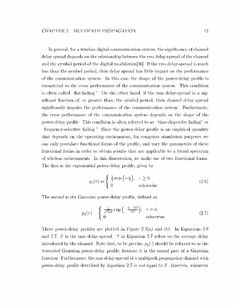
of wireless environments. In this dissertation, we make use of two functional forms.
The �rst is the exponential power-delay pro�le, given by
pe(�) =
8<:
1Sexp
�� �
S
�; � � 0;
0 otherwise.(2.6)
The second is the Gaussian power-delay pro�le, de�ned as
pg(�) =
8<:
1p2�S
exp�� (���� )2
2S2
�; � � 0;
0 otherwise.(2.7)
These power-delay pro�les are plotted in Figure 2.3(a) and (b). In Equations 2.6
and 2.7, S is the rms delay-spread. �� in Equation 2.7 refers to the average delay
introduced by the channel. Note that, to be precise, pg(�) should be referred to as the
truncated Gaussian power-delay pro�le, because it is the causal part of a Gaussian
function. Furthermore, the rms delay-spread of a multipath propagation channel with
power-delay pro�le described by Equation 2.7 is not equal to S. However, whenever
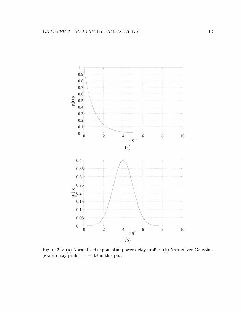
CHAPTER 2. MULTIPATH PROPAGATION 13
-1τ S
)p e(τ
S
20 4 6 8 10
0.9
0.8
0.7
0.6
0.5
0.4
0.3
0.2
0.1
1
0
(a)
-1τ S0 2 4 6 8 10
0.05
0.1
0.15
0.2
0.25
0.3
0.35
0.4
0
)p g(τ
S
(b)
Figure 2.3: (a) Normalized exponential power-delay pro�le. (b) Normalized Gaussian
power-delay pro�le. �� = 4S in this plot.

CHAPTER 2. MULTIPATH PROPAGATION 14
dv
X Y
α
dcos
( )α
Figure 2.4: Illustration of Doppler shift in the free-space propagation environment.
The receiver moves at a constant velocity v along a direction that forms an angle �
with the incident wave.
Equation 2.7 is used in this dissertation, �� is set to a value that is signi�cantly
larger than S. In this case pg(�) is essentially the same as the Gaussian function
before truncation, and the rms delay spread is essentially equal to S. For the sake of
brevity, we will simply refer to pg(�) as the \Gaussian power-delay pro�le."
2.3 Doppler Spread
When a single-frequency sinusoid is transmitted in a free-space propagation envi-
ronment where there is no multipath propagation, the relative motion between the
transmitter and receiver results in an apparent change in the frequency of the received
signal. This apparent frequency change is called Doppler shift. To analyze this e�ect,
consider the simple scenario shown in Figure 2.4. Assuming that the transmitter is
far away so that plane wave approximations hold at the receiver location, and that
the receiver is moving at a constant velocity v along a direction that forms an angle
� with the incident electro-magnetic wave, then it can be seen that the di�erence
in path lengths traveled by the wave from the transmitter to the mobile receiver at
points X and Y is given by
�l = d cos� (2.8)
= v�t cos�; (2.9)
CHAPTER 2. MULTIPATH PROPAGATION 15
where �t is the time required for the mobile to travel from X to Y. The phase change
in the received signal due to the di�erence in path lengths is therefore
�� =2��l
�(2.10)
=2�v�t
�cos�; (2.11)
where � is the wavelength. Hence, the apparent change in received frequency, or
Doppler shift, is given by
fd =1
2�
��
�t(2.12)
=v
�cos� (2.13)
=v
cfc cos�: (2.14)
In Equation 2.14, c is the speed of light and fc is the frequency of the transmitted
sinusoid. In going from Equation 2.13 to 2.14, the relationship
c = fc� (2.15)
is used.
It can be seen from Equation 2.14 that Doppler shift is a function of, among other
parameters, the angle of arrival of the transmitted signal. In a multipath propagation
environment in which multiple signal copies propagate to the receiver with di�erent
angles of arrival, the Doppler shift will be di�erent for di�erent propagation paths.
The resulting signal is the sum of the multipath components. Consequently, the
frequency spectrum of the received signal will in general be \wider" than that of the
transmitted signal, i.e. it contains more frequency components than were transmitted.
This phenomenon is referred to as Doppler spread. Since the received signal occupies
a wider band than the transmitted signal, the multipath propagation channel is a
time-varying linear system when there is relative motion. The amount of Doppler
spread, then, characterizes the rate of channel variations.
Doppler spread can be quantitatively characterized by the Doppler spectrum[1].

CHAPTER 2. MULTIPATH PROPAGATION 16
fcfc fmax- fc fmax+f
K
S(f)
Figure 2.5: The Doppler spectrum corresponding to uniformly distributed angles of
arrival (see Equation 2.16).
The Doppler spectrum is the power spectral density of the received signal when a
single-frequency sinusoid is transmitted over a multipath propagation channel. In a
static environment in which the re ectors stay immobile, the Doppler spectrum is
simply an impulse located at the frequency of the transmitted sinusoid when there
is no relative motion. When there is relative motion, the Doppler spectrum occupies
a �nite bandwidth. The exact shape of the Doppler spectrum depends on the con-
�guration of the re ectors. It can be shown[1] that when the mobile receiver moves
at a constant speed v and the signal power received by the receiver antenna arrives
uniformly from all incident angles in [0; 2�), the Doppler spectrum takes a form of
S(f) =Kr
1��f�fcfmax
�2 ; (2.16)
whereK is a proportionality constant and fmax = (vc)fc is the maximumDoppler shift.
This Doppler spectrum is plotted in Figure 2.5. In reality, however, the exact shape
of the Doppler spectrum can only be obtained by extensive �eld measurements, and
Equation 2.16 is approximately true only in certain environments. The bandwidth of
the Doppler spectrum, or equivalently the maximum Doppler shift fmax, is a measure
CHAPTER 2. MULTIPATH PROPAGATION 17
of the rate of channel variations. When the Doppler bandwidth is small compared
to the bandwidth of the signal, the channel variations are slow relative to the signal
variations. This is often referred to as \slow fading." On the other hand, when the
Doppler bandwidth is comparable to or greater than the bandwidth of the signal, the
channel variations are as fast or faster than the signal variations. This is often called
\fast fading."
2.4 Baseband Indoor Wireless Channel Model
The focus of this dissertation is on the mitigation of small-scale e�ects due to mul-
tipath propagation in indoor wireless channels. Indoor wireless channels di�er from
the traditional outdoor mobile radio channels in several aspects. First, the multi-
path structure is of a much smaller scale. In other words, the re ectors in indoor
environments are much more closed-in than those in outdoor environments. Con-
sequently the rms delay spread is much smaller for indoor environments. The rms
delay-spreads of indoor wireless channels typically range from 10 to 100 ns. This is
signi�cantly smaller than the typical values of 1.5 to 5 �s in outdoor environments.
Secondly, indoor wireless channels vary very slowly. A mobile moving at 6 km/hour
{ a fast walking speed { results in a maximum Doppler shift of 5 Hz when the carrier
frequency is 900 MHz. Secondary e�ects, such as motion of people and doors being
opened and closed, also contribute to channel variations. However, the variations
due to these secondary e�ects are also very slow[18]. In contrast, in outdoor cellular
environments, a vehicle traveling at 120 km/hour results in a maximum Doppler shift
of 100 Hz when the carrier frequency is 900 MHz, which is signi�cantly higher than
that of indoor wireless channels.
Based on the discussions presented in Sections 2.1-2.3, we have adopted the fol-
lowing baseband model for indoor wireless channels. Assuming that a (baseband
equivalent) signal u(t) is transmitted over an indoor wireless channel, the baseband

CHAPTER 2. MULTIPATH PROPAGATION 18
representation of the received signal r(t) is given by
r(t) =MX
m=1
amu(t� �m)ej�me�j!c�mej!mt + n(t); (2.17)
where !c and M are the carrier frequency and number of multipath components,
respectively, and j =p�1. famg, f�mg, f�mg and f!mg are the path gains, phases,
delays and Doppler shift frequencies, respectively, of the channel. n(t) is the addi-
tive white Gaussian noise (AWGN). These parameters are assumed to be mutually
independent. The path gains famg are assumed to be i.i.d. according to the Rayleigh
distribution, with the constraint that
E
"MX
m=1
a2m
#= 1: (2.18)
The path phases f�mg are assumed to be i.i.d. uniformly in [0; 2�). We assume that
the Doppler shift frequency of the each path is proportional to the cosine of the
corresponding angle of arrival (see Equation 2.14). Furthermore, we also assume that
the angles of arrival of the propagation paths are i.i.d. uniformly in [0; 2�): As a result,
f!mg are distributed according to the inverse-cosine distribution, whose probability
density function is given by
f(!) =
8><>:
1p(!�!max)2
j!j < !max;
0 otherwise;(2.19)
where !max = 2�fmax: Throughout this dissertation, we will assume that fmax = 5
Hz. The number of paths M is set to 20, and the carrier frequency !c is �xed at
2��900 Mrad/sec. Note that the latter assumption, together with the distribution
of the Doppler frequencies, correspond to a mobile speed of 1.67 meters/sec, which is
reasonable for indoor applications.
Two points are worth noting for this channel model. First, it can be shown
that the power-delay pro�le of this channel model is proportional to the probability
density function of the path delays f�mg. The standard deviation of the path delays
CHAPTER 2. MULTIPATH PROPAGATION 19
Param Meaning Statistics
!c Carrier Freq. 2��900 Mrad/sec
M Num. of Paths 20
famg Path Gains Rayleigh; E[P
M
m=1 a2m] = 1
f�mg Path Delays Exponential with std. dev. of 50ns; OR
Gaussian with mean 200ns and std. dev. 50ns
f�mg Path Phases Uniform in [0; 2�)
f!mg Doppler Shift Freq. Inverse-cosine in [�2� � 5; 2� � 5] rad/sec
fn(t)g Noise Complex WGN
Table 2.1: Channel parameters used throughout this dissertation.
is therefore the rms delay-spread of the channel. A proof is given in Appendix A. It
is, therefore, possible to simulate wireless channels with arbitrarily given power-delay
pro�les by using the channel model described in this section. As mentioned previously,
in this dissertation we assume that the channel power-delay pro�le is either Gaussian
or exponential. Furthermore, we assume that the indoor wireless channel has a rms
delay spread of 50 ns. For the Gaussian power-delay pro�le, we also assume that
the average delay �� = 200ns, i.e. four times the rms delay-spread. This implies that
the path delays f�mg are either i.i.d. Gaussianly or i.i.d. exponentially distributed
with a standard deviation of 50 ns. For the Gaussian case, the mean is set to 200
ns. Secondly, it can also be shown that the Doppler spectrum is proportional to the
distribution of the Doppler shift frequencies f!mg. This is proved in Appendix B.
Therefore, it is also possible to specify arbitrarily the Doppler spectrum of this channel
model. As mentioned previously, throughout this dissertation we assume that f!mgare distributed according to an inverse-cosine distribution. The Doppler spectrum is,
therefore, proportional to the probability density function given in Equation 2.19.
The meanings and statistics of these parameters are summarized in Table 2.1. It
should be noted that although the channel model and the corresponding parameters
that we have adopted are reasonably realistic, they are used only for the purpose of
evaluating the relative performance of di�erent multipath mitigation techniques. If
the absolute performance in a particular environment is to be predicted, di�erent sets
of parameters, or even a di�erent channel model, should be extracted from extensive
CHAPTER 2. MULTIPATH PROPAGATION 20
�eld measurements taken in the environment in question.
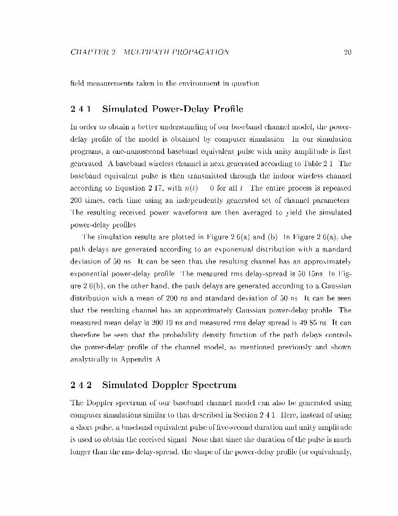
2.4.1 Simulated Power-Delay Pro�le
In order to obtain a better understanding of our baseband channel model, the power-
delay pro�le of the model is obtained by computer simulation. In our simulation
programs, a one-nanosecond baseband equivalent pulse with unity amplitude is �rst
generated. A baseband wireless channel is next generated according to Table 2.1. The
baseband equivalent pulse is then transmitted through the indoor wireless channel
according to Equation 2.17, with n(t) = 0 for all t. The entire process is repeated
200 times, each time using an independently generated set of channel parameters.
The resulting received power waveforms are then averaged to yield the simulated
power-delay pro�les.
The simulation results are plotted in Figure 2.6(a) and (b). In Figure 2.6(a), the
path delays are generated according to an exponential distribution with a standard
deviation of 50 ns. It can be seen that the resulting channel has an approximately
exponential power-delay pro�le. The measured rms delay-spread is 50.15ns. In Fig-
ure 2.6(b), on the other hand, the path delays are generated according to a Gaussian
distribution with a mean of 200 ns and standard deviation of 50 ns. It can be seen
that the resulting channel has an approximately Gaussian power-delay pro�le. The
measured mean delay is 200.19 ns and measured rms delay-spread is 49.85 ns. It can
therefore be seen that the probability density function of the path delays controls
the power-delay pro�le of the channel model, as mentioned previously and shown
analytically in Appendix A.
2.4.2 Simulated Doppler Spectrum
The Doppler spectrum of our baseband channel model can also be generated using
computer simulations similar to that described in Section 2.4.1. Here, instead of using
a short pulse, a baseband equivalent pulse of �ve-second duration and unity amplitude
is used to obtain the received signal. Note that since the duration of the pulse is much
longer than the rms delay-spread, the shape of the power-delay pro�le (or equivalently,

CHAPTER 2. MULTIPATH PROPAGATION 21
0 50 100 150 200 250Delay (ns)
0.025
0.005
0.01
0.015
0.02
0
Pow
er (
W)
(a)
0 100 200 300 400 500
0.002
0.004
0.006
0.008
0.01
0.012
0
Pow
er (
W)
Delay (ns)
(b)
Figure 2.6: Simulated power-delay pro�les obtained from 200 replications. (a) The
path delays are exponentially distributed with a standard deviation of 50 ns. (b) The
path delays are Gaussianly distributed with a mean of 200 ns and standard deviation
of 50 ns.

CHAPTER 2. MULTIPATH PROPAGATION 22
0.1
0
0.2
0.3
0.4
0.5
0.6
0.7
Pow
er D
ensi
ty (
W/H
z)
-10 -5 0 5 10Doppler Frequency (Hz)
Figure 2.7: Simulated Doppler spectrum obtained from 200 replications. The Doppler
shift frequencies are generated according to Table 2.1
the distribution of the path delays) is immaterial. The received baseband equivalent
power spectrum, i.e. the squared magnitude of the Fourier transform of the received
signal, is next computed. The simulated Doppler spectrum is then the average of the
replicated baseband equivalent power spectra. The simulation results are plotted in
Figure 2.7. It can be seen that the simulated Doppler spectrum has a shape similar
to that shown in Figure 2.5. Furthermore, the received signal power is approximately
con�ned to �5 Hz. This is expected because, as mentioned previously and shown
in Appendix B, the baseband equivalent Doppler spectrum of our channel model
is proportional to the distribution of the path Doppler shift frequencies given in
Equation 2.19. However, Equation 2.19 is of the same functional form as the Doppler
spectrum given in Equation 2.16, which is plotted in Figure 2.5. It is therefore
veri�ed that the Doppler spectrum of our channel model can be controlled by properly
specifying the distribution of the path Doppler shift frequencies.

CHAPTER 2. MULTIPATH PROPAGATION 23
2.5 Summary
Due to the presence of re ectors and scatterers in the environment, the signal trans-
mitted through a wireless radio channel propagates to the receiver antenna via many
di�erent paths. The output of the receiver antenna is, therefore, a sum of many
distorted copies of the transmitted signal. These copies generally have di�erent am-
plitudes, time delays, phase shifts, and angles of arrival. This phenomenon is referred
to as multipath propagation.
The e�ect of multipath propagation can be classi�ed into large-scale and small-
scale variations. Small-scale variations include signal fading, delay spread, and Doppler
spread. Signal fading refers to the rapid change in received signal strength over a small
travel distance or time interval. It occurs because of the constructive and destructive
interference between signal copies. Delay spread refers to the smearing or widening
of a short pulse transmitted through a multipath propagation channel. It happens
because di�erent propagation paths have di�erent time delays. Doppler spread refers
to the widening of the spectrum of a narrow-band signal transmitted through a mul-
tipath propagation channel. It is due to the di�erent Doppler shift frequencies asso-
ciated with the multiple propagation paths when there is relative motion between the
transmitter and receiver. These small-scale e�ects can be quantitatively characterized
using the signal amplitude distribution, power-delay pro�le and rms delay-spread, and
Doppler spectrum. All these characterizations are empirical statistics that must be
obtained using extensive �eld measurements.
Based on the qualitative description of multipath propagation and some empirical
data found in the literature, we have adopted a simple baseband model for indoor
wireless radio channels. This model is described in Section 2.4. The power-delay
pro�le and Doppler spectrum of this channel model can be controlled by properly
specifying the distribution of some model parameters. Simulation results are shown
in Sections 2.4.1 and 2.4.2 to demonstrate the exibility of this channel model. This
channel model will be used in all simulations in this dissertation.
Chapter 3
Adaptive Decision-Feedback
Equalization
As mentioned in Chapter 2, delay spread is one of the e�ects of multipath propagation.
In an environment where delay spread is signi�cant, high-speed data transmission
encounters inter-symbol interference, which can drastically impair the performance
of a data communication system. One technique for mitigating the e�ect of delay
spread is adaptive equalization. An adaptive equalizer is a special form of adaptive
�lter which, when designed and optimized correctly, can remove most of the inter-
symbol interference present in the received signal. In this chapter, we describe in
detail inter-symbol interference and adaptive equalization.
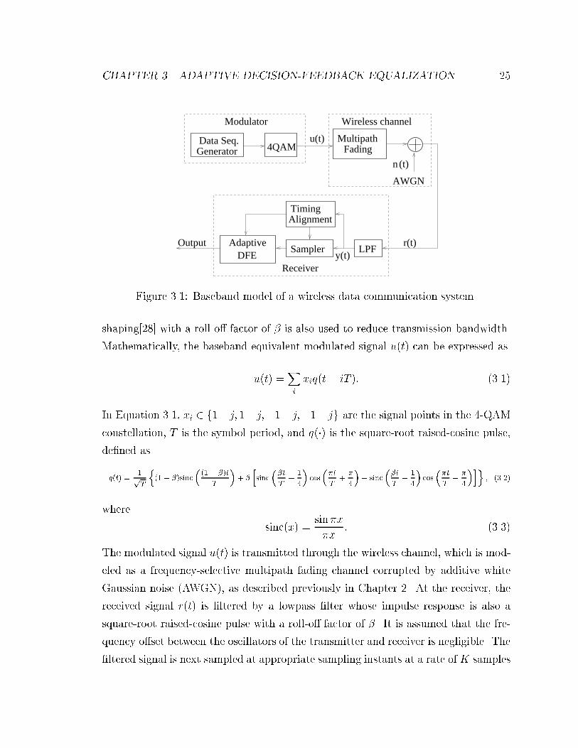
3.1 System Model
Consider the wireless data communication system shown in Figure 3.1. The sys-
tem consists of the digital modulator, wireless channel, and receiver. As shown in
Figure 3.1, the digital modulator consists of a binary data sequence generator and
an uncoded 4-QAM modulator[27]. The binary data sequence generator generates a
binary data stream with equally likely 0's and 1's. Successive symbols in this data
stream are assumed to be independent. This data sequence is coherently modu-
lated onto the carrier by the 4-QAM modulator. Square-root raised-cosine spectral
24
CHAPTER 3. ADAPTIVE DECISION-FEEDBACK EQUALIZATION 25
Data Seq. Generator 4QAM
Wireless channel
(t)n
AWGN
MultipathFading
TimingAlignment
LPFSampler
Receiver
r(t)Output
u(t)
y(t)DFEAdaptive
Modulator
Figure 3.1: Baseband model of a wireless data communication system.
shaping[28] with a roll-o� factor of � is also used to reduce transmission bandwidth.
Mathematically, the baseband equivalent modulated signal u(t) can be expressed as
u(t) =Xi
xiq(t� iT ): (3.1)
In Equation 3.1, xi 2 f1+ j; 1� j;�1+ j;�1� jg are the signal points in the 4-QAMconstellation, T is the symbol period, and q(�) is the square-root raised-cosine pulse,de�ned as
q(t) =1pT
n(1� �)sinc
�(1� �)t
T
�+ �
hsinc
��t
T+
1
4
�cos
��t
T+
�
4
�+ sinc
��t
T�
1
4
�cos
��t
T�
�
4
�io; (3.2)
where
sinc(x) =sin�x
�x: (3.3)
The modulated signal u(t) is transmitted through the wireless channel, which is mod-
eled as a frequency-selective multipath fading channel corrupted by additive white
Gaussian noise (AWGN), as described previously in Chapter 2. At the receiver, the
received signal r(t) is �ltered by a lowpass �lter whose impulse response is also a
square-root raised-cosine pulse with a roll-o� factor of �. It is assumed that the fre-
quency o�set between the oscillators of the transmitter and receiver is negligible. The
�ltered signal is next sampled at appropriate sampling instants at a rate of K samples
CHAPTER 3. ADAPTIVE DECISION-FEEDBACK EQUALIZATION 26
per symbol-period. The sampling instants are determined by the \timing alignment"
algorithm[29], which will be described in Chapter 4. The resulting discrete-time signal
is fed into the adaptive decision-feedback equalizer to yield the demodulated output.
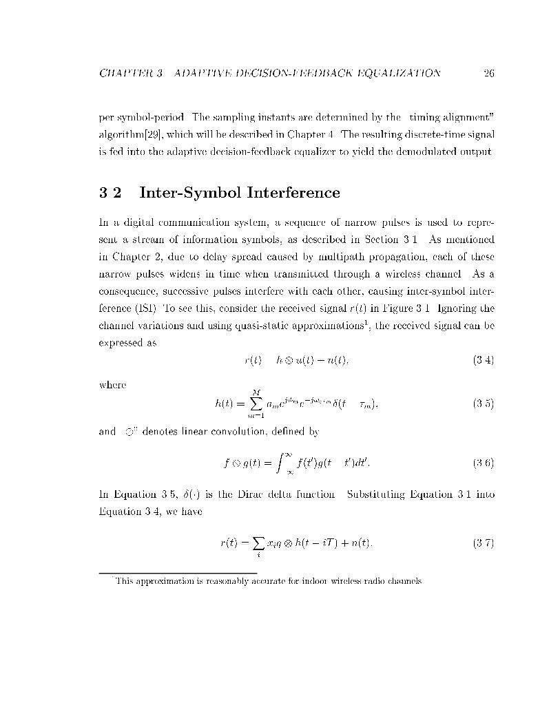
3.2 Inter-Symbol Interference
In a digital communication system, a sequence of narrow pulses is used to repre-
sent a stream of information symbols, as described in Section 3.1. As mentioned
in Chapter 2, due to delay spread caused by multipath propagation, each of these
narrow pulses widens in time when transmitted through a wireless channel. As a
consequence, successive pulses interfere with each other, causing inter-symbol inter-
ference (ISI). To see this, consider the received signal r(t) in Figure 3.1. Ignoring the
channel variations and using quasi-static approximations1, the received signal can be
expressed as
r(t) = h u(t) + n(t); (3.4)
where
h(t) =MX
m=1
amej�me�j!c�m�(t� �m); (3.5)
and \" denotes linear convolution, de�ned by
f g(t) =
Z 1
�1f(t0)g(t� t0)dt0: (3.6)
In Equation 3.5, �(�) is the Dirac delta function. Substituting Equation 3.1 into
Equation 3.4, we have
r(t) =Xi
xiq h(t� iT ) + n(t): (3.7)
1This approximation is reasonably accurate for indoor wireless radio channels.

CHAPTER 3. ADAPTIVE DECISION-FEEDBACK EQUALIZATION 27
As shown in Figure 3.1, the received signal is passed through a �lter with impulse
response q(�). Thus, the output of the �lter is
y(t) = r q(t) (3.8)
=Xi
xiq h q(t� iT ) + n q(t): (3.9)
Finally, the signal y(t) is sampled at proper instants to yield the discrete-time signal
yj. Assume, for the time being, that K = 1 sample is taken per symbol period. Then,
we have
yj = y(jT + �); j = 0; 1; 2; : : : (3.10)
=Xi
xiq h q ((j � i)T + �) + n q(jT + �); (3.11)
where � is the time at which the �rst sample is taken. Let
p(t) = q h q(t) (3.12)
and
pi = p(iT + �); (3.13)
ni = n q(iT + �); (3.14)
then
yj =Xi
xipj�i + nj (3.15)
= p0xj +Xi6=j
xipj�i + nj: (3.16)
It can thus be seen that if pj = 0 for all j 6= 0, then the �ltered received signal
yj is simply a scaled version of the transmitted symbol corrupted by additive �ltered
Gaussian noise. However, in general with delay spread pj 6= 0 even when j 6= 0,
thus the discrete-time signal yj contains not only the contribution from the \current"

CHAPTER 3. ADAPTIVE DECISION-FEEDBACK EQUALIZATION 28
symbol xj (given by the �rst term, p0xj, in Equation 3.16), but also contributions
from \previous" and \future" symbols (P
i6=j xipj�i) and �ltered Gaussian noise (nj).
The second term in Equation 3.16 is the ISI. It is the weighted sum of previous and
future symbols, with weights taken from fpig. pi is an important quantity that plays
the key role in characterizing ISI, and will be referred to as the channel pulse response
(CPR) in this dissertation. As can be seen in Equation 3.12 and 3.13, the CPR is
simply the sampled version of the response of the channel to the transmitted pulse
after being �ltered by the receive �lter.
The above analysis can be extended to the case where more than one sample is
take per symbol-period. Assuming that the signal y(t) is sampled at a rate of K
samples per symbol-period, where K is assumed to be an integer. These samples are
denoted as
yj;k = y(jT + � � kT
K) (3.17)
=Xi
xip
(j � i)T + � � kT
K
!+ n q
jT + � � kT
K
!; (3.18)
where j = 0; 1; : : :, and k = 0; 1; : : : ; (K � 1). Let
pi;k = p
iT + � � kT
K
!; (3.19)
and
ni;k = n q
iT + � � kT
K
!; (3.20)
then
yj;k =Xi
xipj�i;k + nj;k (3.21)
for k = 0; 1; : : : ; (K � 1). We can combine Equations 3.19, 3.20 and 3.21 into a more
CHAPTER 3. ADAPTIVE DECISION-FEEDBACK EQUALIZATION 29
compact form given by
yj =
26666664
yj;0
yj;1
: : :
yj;K�1
37777775
(3.22)
=Xi
xipj�i + nj (3.23)
= p0xj +Xi6=j
xipj�i + nj: (3.24)
where
pi =
26666664
pi;0
pi;1
: : :
pi;K�1
37777775; (3.25)
and
nj =
26666664
nj;0
nj;1
: : :
nj;K�1
37777775: (3.26)
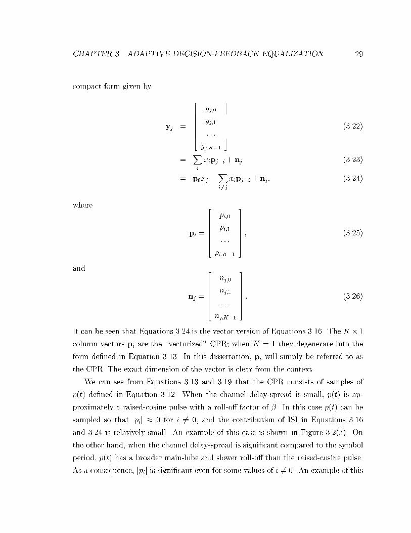
It can be seen that Equations 3.24 is the vector version of Equations 3.16. The K�1
column vectors pi are the \vectorized" CPR; when K = 1 they degenerate into the
form de�ned in Equation 3.13. In this dissertation, pi will simply be referred to as
the CPR. The exact dimension of the vector is clear from the context.
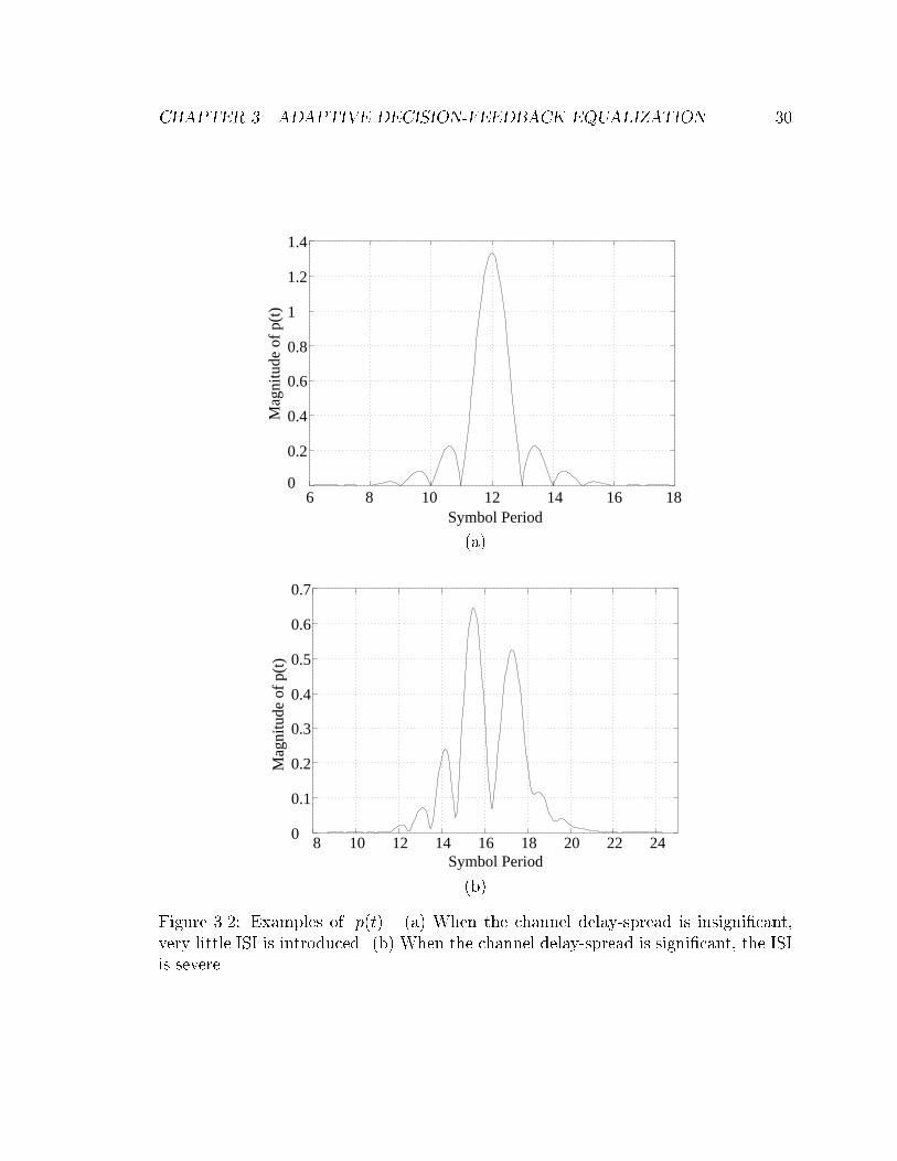
We can see from Equations 3.13 and 3.19 that the CPR consists of samples of
p(t) de�ned in Equation 3.12. When the channel delay-spread is small, p(t) is ap-
proximately a raised-cosine pulse with a roll-o� factor of �. In this case p(t) can be
sampled so that jpij � 0 for i 6= 0, and the contribution of ISI in Equations 3.16
and 3.24 is relatively small. An example of this case is shown in Figure 3.2(a). On
the other hand, when the channel delay-spread is signi�cant compared to the symbol
period, p(t) has a broader main-lobe and slower roll-o� than the raised-cosine pulse.
As a consequence, jpij is signi�cant even for some values of i 6= 0. An example of this
CHAPTER 3. ADAPTIVE DECISION-FEEDBACK EQUALIZATION 30
1.4
1.2
1
0.8
0.6
0.4
0.2
06 8 10 12 14 16 18
Symbol Period
Mag
nitu
de o
f p(
t)
(a)
108 12 14 16 18 20 22 24
0.7
0.6
0.5
0.4
0.3
0.2
0.1
0
Symbol Period
Mag
nitu
de o
f p(
t)
(b)
Figure 3.2: Examples of jp(t)j. (a) When the channel delay-spread is insigni�cant,
very little ISI is introduced. (b) When the channel delay-spread is signi�cant, the ISI
is severe.
CHAPTER 3. ADAPTIVE DECISION-FEEDBACK EQUALIZATION 31
Tap-Wt.Adapt
xj
+FeedforwardFilter
FeedbackFilterDFE
zj∆y
j+y
j
AlignmentTiming
FilterReceiver r(t)
τ ∆Advance
Sample∆y(t)
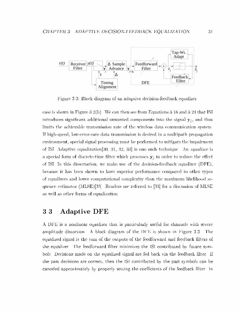
Figure 3.3: Block diagram of an adaptive decision-feedback equalizer.
case is shown in Figure 3.2(b). We can then see from Equations 3.16 and 3.24 that ISI
introduces signi�cant additional unwanted components into the signal yj, and thus
limits the achievable transmission rate of the wireless data communication system.
If high-speed, low-error-rate data transmission is desired in a multipath propagation
environment, special signal processing must be performed to mitigate the impairment
of ISI. Adaptive equalization[30, 31, 32, 33] is one such technique. An equalizer is
a special form of discrete-time �lter which processes yj in order to reduce the e�ect
of ISI. In this dissertation, we make use of the decision-feedback equalizer (DFE),
because it has been shown to have superior performance compared to other types
of equalizers and lower computational complexity than the maximum likelihood se-
quence estimator (MLSE)[33]. Readers are referred to [33] for a discussion of MLSE
as well as other forms of equalization.
3.3 Adaptive DFE
A DFE is a nonlinear equalizer that is particularly useful for channels with severe
amplitude distortion. A block diagram of the DFE is shown in Figure 3.3. The
equalized signal is the sum of the outputs of the feedforward and feedback �lters of
the equalizer. The feedforward �lter minimizes the ISI contributed by future sym-
bols. Decisions made on the equalized signal are fed back via the feedback �lter. If
the past decisions are correct, then the ISI contributed by the past symbols can be
canceled approximately by properly setting the coe�cients of the feedback �lter. In

CHAPTER 3. ADAPTIVE DECISION-FEEDBACK EQUALIZATION 32
this dissertation, we use linear �nite-impulse-response (FIR) feedforward and feed-
back �lters with Nf and Nb taps, respectively. Linear FIR �lters are chosen to make
the adaptation algorithms simpler[34]. The DFE can then be regarded as an esti-
mator which uses the linear combination of the components of the �ltered received
signal samples yj+�;yj+��1; : : : ;yj+��Nf+1 and past decisions x̂j�1; x̂j�2; : : : ; x̂j�Nb
to estimate the transmitted symbol xj. The integer � is the \decision delay" of the
DFE[29, 35, 36, 37]. It re ects the signal spread introduced by multipath propaga-
tion and controls the trade-o� between time diversity and ISI. The performance of
the DFE is very sensitive to the choice of �, especially when the number of taps in
the feedforward �lter is small. Optimization of � is discussed in Chapter 4.
The DFE �lter coe�cients are jointly optimized according to some optimization
criterion. For the equalization of wireless channels, it is desirable to adapt, or re-
compute, the DFE �lter coe�cients on a symbol-by-symbol basis. First, wireless
channels are time-varying channels, therefore the optimal DFE �lter coe�cients vary
with time. Secondly, although indoor wireless channels vary very slowly, they are ran-
dom channels that are di�erent in di�erent environments. Therefore, the DFE must
be self-synthesizing, so that the �lter coe�cients can automatically adapt to the en-
vironment in which the DFE operates. DFE's whose �lter coe�cients are optimized
on a symbol-by-symbol basis are called adaptive DFE's. Mathematically, the output
(equalized signal) z(j; k) of an adaptive DFE at time j using the �lter coe�cients
obtained at time k can be expressed as2
z(j; k) =
Nf�1Xi=0
w�i;kyj+��i +
NbXi=1
b�i;kx̂j�i; (3.27)
where wi;k are K � 1 feedforward coe�cient vectors and bi;k are the feedback coe�-
cients, both optimized at time k. Equation 3.27 can be expressed in a more compact
form given by
z(j; k) = [w�k;b�
k]Yj+�; (3.28)
2\*" denotes the Hermitian transposition.

CHAPTER 3. ADAPTIVE DECISION-FEEDBACK EQUALIZATION 33
where
wk =
26666664
w0;k
w1;k
� � �wNf�1;k
37777775; (3.29)
bk =
26666664
b1;k
b2;k
� � �bNb;k
37777775; (3.30)
and
Yj+� =
266666666666666666664
yj+�
yj+��1
: : :
yj+��Nf+1
x̂j�1
x̂j�2
: : :
x̂j�Nb
377777777777777777775
: (3.31)
The �lter coe�cients wk and bk are jointly optimized using adaptation approaches
to be described in Section 3.3.1 and 3.3.2. The \one-step output" zj = z(j; j � 1) is
used to produced the detected symbol x̂j:
3.3.1 Channel Estimation Based Adaptation
The channel estimation based adaptation (CEBA) is an indirect approach for opti-
mizing the DFE �lter coe�cients. In this approach, an estimate of the CPR is �rst
obtained using channel estimation algorithms, e.g. the recursive least-squares (RLS)
algorithm[38, 42]. The DFE �lter coe�cients are next computed as a function of
these CPR estimates. This process is repeated once every symbol-period. It should
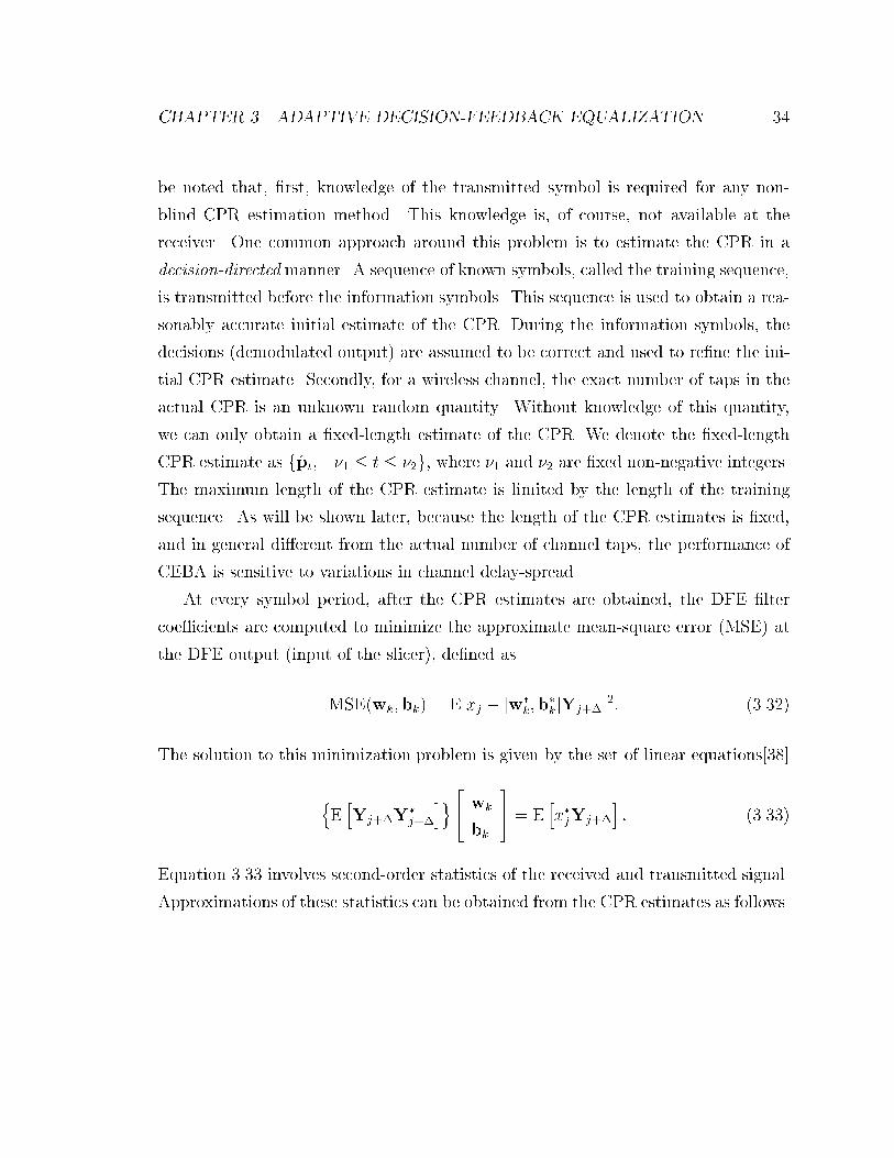
CHAPTER 3. ADAPTIVE DECISION-FEEDBACK EQUALIZATION 34
be noted that, �rst, knowledge of the transmitted symbol is required for any non-
blind CPR estimation method. This knowledge is, of course, not available at the
receiver. One common approach around this problem is to estimate the CPR in a
decision-directedmanner. A sequence of known symbols, called the training sequence,
is transmitted before the information symbols. This sequence is used to obtain a rea-
sonably accurate initial estimate of the CPR. During the information symbols, the
decisions (demodulated output) are assumed to be correct and used to re�ne the ini-
tial CPR estimate. Secondly, for a wireless channel, the exact number of taps in the
actual CPR is an unknown random quantity. Without knowledge of this quantity,
we can only obtain a �xed-length estimate of the CPR. We denote the �xed-length
CPR estimate as fp̂t;��1 � t � �2g, where �1 and �2 are �xed non-negative integers.
The maximum length of the CPR estimate is limited by the length of the training
sequence. As will be shown later, because the length of the CPR estimates is �xed,
and in general di�erent from the actual number of channel taps, the performance of
CEBA is sensitive to variations in channel delay-spread.
At every symbol period, after the CPR estimates are obtained, the DFE �lter
coe�cients are computed to minimize the approximate mean-square error (MSE) at
the DFE output (input of the slicer), de�ned as
MSE(wk;bk) = Ejxj � [w�k;b�
k]Yj+�j2: (3.32)
The solution to this minimization problem is given by the set of linear equations[38]
nEhYj+�Y
�j+�
io 24 wk
bk
35 = E
hx�jYj+�
i: (3.33)
Equation 3.33 involves second-order statistics of the received and transmitted signal.
Approximations of these statistics can be obtained from the CPR estimates as follows.

CHAPTER 3. ADAPTIVE DECISION-FEEDBACK EQUALIZATION 35
First, assuming that the past decisions are correct, we have3
Yj+� = ~PXj+�1 +
24 Nj+�
0Nb
35 ; (3.34)
where
~P =
24 P
0Nb;�1+1 INb0Nb;�2+Nf�Nb�1
35 ; (3.35)
Xj+�1 =
26666664
xj+�1
xj+�1�1
: : :
xj��2�Nf+1
37777775; (3.36)
Nj+� =
26666664
nj+�
nj+��1
: : :
nj+��Nf+1
37777775; (3.37)
0a denotes an a� 1 column vector of zeros, INbdenotes an identity matrix of size Nb,
and 0a;b denotes an a�b block of zeros. In Equation 3.35, P is a NfK�(�1+�2+Nf )
matrix composed ofNf rows of column vectors, each withK components. Speci�cally,
P is de�ned as
P =
26666664
p̂��1+� p̂��1+1+� � � � p̂�2+� 0K 0K � � � 0K
0K p̂��1+� p̂��1+1+� � � � p̂�2+� 0K � � � 0K
� � � � � � � � � � � � � � � � � � � � � � � �0K 0K � � � 0K p̂��1+� p̂��1+1+� � � � p̂�2+�
37777775:
(3.38)
Thus,
EhYj+�Y
�j+�
i= ~P
nEhXj+�X
�j+�
io~P� + E
8<:24 Nj+�
0Nb
35 h N�
j+� 0�Nb
i9=; ; (3.39)
3This is actually only an approximation because of the inaccuracy in estimating the CPR.

CHAPTER 3. ADAPTIVE DECISION-FEEDBACK EQUALIZATION 36
and
Ehx�jYj+�
i= ~PE
hx�jXj+�
i: (3.40)
Making use of the assumption that successive transmitted symbols are independent
of each other, we have
EhXj+�X
�j+�
i= 2I�1+�2+Nf
; (3.41)
thus
EhYj+�Y
�j+�
i= 2
24 PP� +RN H
H� INb
35 ; (3.42)
where
H = P
26664
0�1+1;Nb
INb
0�2+Nf�Nb�1;Nb
37775 ; (3.43)
and
RN =1
2EhNj+�N
�j+�
i: (3.44)
Furthermore,
Ehx�jXj+�
i= 2e�1; (3.45)
where e�1 denotes a (�1+ �2+Nf )� 1 column vector with a one in the �1-th position
and zeros elsewhere. Thus,
Ehx�jYj+�
i= 2~Pe�1 : (3.46)
Substituting Equations 3.42 and 3.46 into Equation 3.33, we have
24 PP� +RN H
H� INb
3524 wk
bk
35 = ~Pe�1 (3.47)
It can be seen from Equation 3.35 that the last Nb elements of the column vector ~Pe�1
are zeros. Therefore the DFE �lter coe�cients, optimal within the approximations,
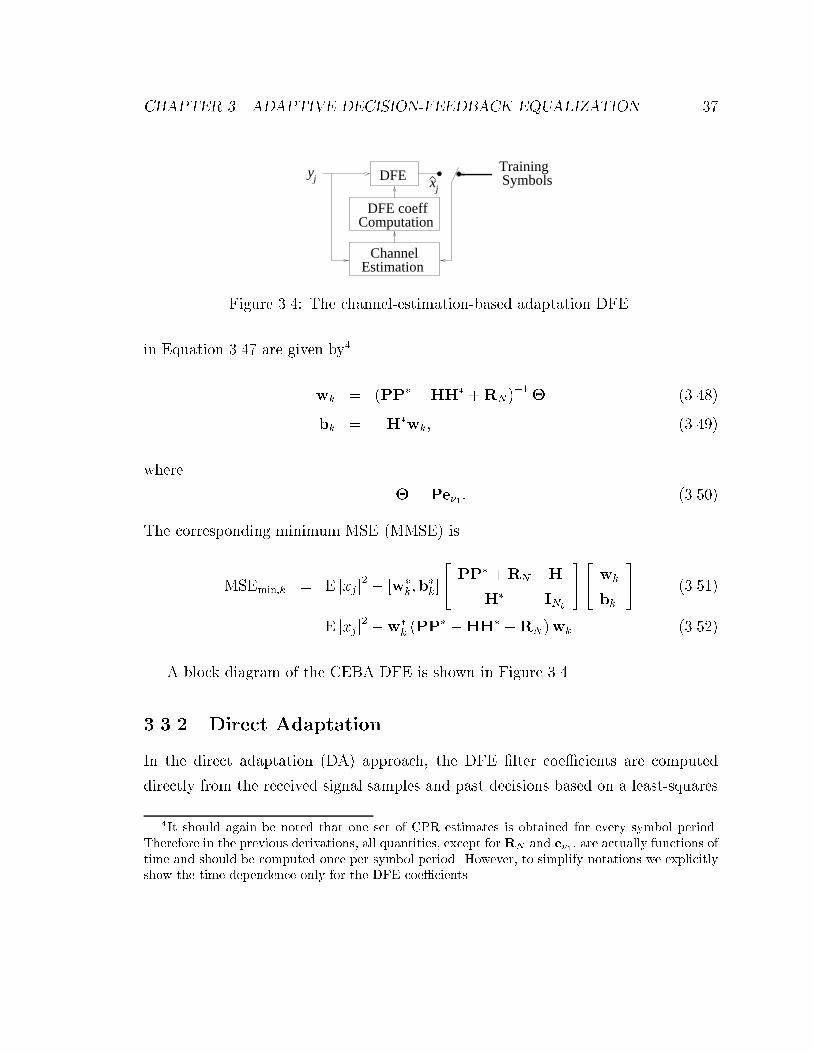
CHAPTER 3. ADAPTIVE DECISION-FEEDBACK EQUALIZATION 37
DFE coeffComputation
ChannelEstimation
Training Symbolsyj
jxDFE
Figure 3.4: The channel-estimation-based adaptation DFE.
in Equation 3.47 are given by4
wk = (PP� �HH� +RN)�1� (3.48)
bk = �H�wk; (3.49)
where
� = Pe�1: (3.50)
The corresponding minimum MSE (MMSE) is
MSEmin;k = E jxjj2 � [w�k;b�
k]
24 PP� +RN H
H� INb
3524 wk
bk
35 (3.51)
= E jxjj2 �w�k(PP� �HH� +RN)wk (3.52)
A block diagram of the CEBA DFE is shown in Figure 3.4.
3.3.2 Direct Adaptation
In the direct adaptation (DA) approach, the DFE �lter coe�cients are computed
directly from the received signal samples and past decisions based on a least-squares
4It should again be noted that one set of CPR estimates is obtained for every symbol period.
Therefore in the previous derivations, all quantities, except for RN and e�1 , are actually functions of
time and should be computed once per symbol period. However, to simplify notations we explicitly
show the time-dependence only for the DFE coe�cients.
CHAPTER 3. ADAPTIVE DECISION-FEEDBACK EQUALIZATION 38
criterion. The exponentially-weighted square output error (WSE) Jk, de�ned as
Jk =kX
j=0
�k�j jz(j; k)� xjj2 ; (3.53)
is minimized at every time k. In Equation 3.53 the \forgetting factor" � is a positive
real number less than but close to 1. As in any other non-blind adaptive algorithm,
a training sequence is required to initialize the DA DFE. When evaluating Equa-
tion 3.53, only those xj that correspond to the training sequence are known to the
receiver. Whenever xj is unknown Jk is evaluated from Equation 3.53 by substituting
x̂j for xj. Since the training sequence consists of symbols known both to the receiver
and the transmitter, it contains no information and is a transmission overhead. It is
therefore desirable to minimize the number of training symbols needed to maintain
an acceptable performance. A simple technique for synthesizing additional training
symbols from the available training sequence will be presented later in this section.
The DA approach di�ers from the CEBA approach in that it is purely determin-
istic. The least-squares criterion in Equation 3.53 does not involve any statistics.
Consequently, no knowledge is assumed about the received signal statistics when
computing the DFE �lter coe�cients. Recall that in the CEBA approach, channel
estimation was done as an intermediate step; the CPR estimates are used to obtain
approximations of the second-order statistics of the received signal. Here, in the DA
approach, channel estimation is not necessary in the computation of the DFE �lter
coe�cients because no statistics are used. As will be shown later by simulation, di-
rectly adapting the DFE �lter coe�cients without going through channel estimation
makes the DA approach more robust against variations in channel delay-spread.
Numerous recursive algorithms[38] are available to minimize Jk. In this disserta-
tion we use the exponentially-weighted least-squares lattice (LSL) algorithm[39, 40]
because of its superior numerical stability and computational e�ciency[40]. A brief
description of the LSL DFE algorithm is given in Appendix C.
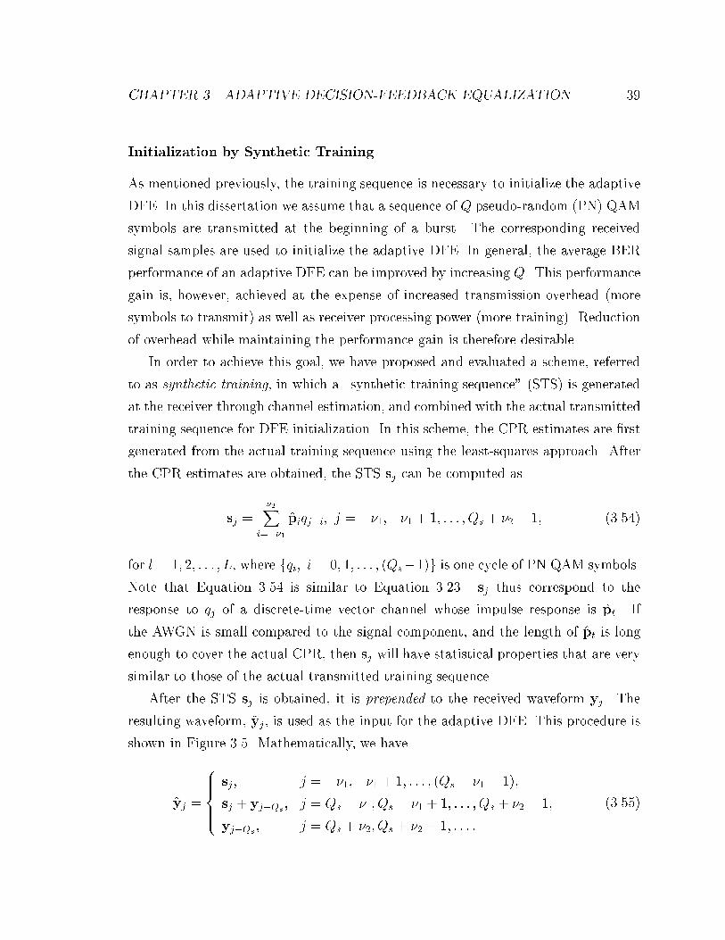
CHAPTER 3. ADAPTIVE DECISION-FEEDBACK EQUALIZATION 39
Initialization by Synthetic Training
As mentioned previously, the training sequence is necessary to initialize the adaptive
DFE. In this dissertation we assume that a sequence of Q pseudo-random (PN) QAM
symbols are transmitted at the beginning of a burst. The corresponding received
signal samples are used to initialize the adaptive DFE. In general, the average BER
performance of an adaptive DFE can be improved by increasing Q. This performance
gain is, however, achieved at the expense of increased transmission overhead (more
symbols to transmit) as well as receiver processing power (more training). Reduction
of overhead while maintaining the performance gain is therefore desirable.
In order to achieve this goal, we have proposed and evaluated a scheme, referred
to as synthetic training, in which a \synthetic training sequence" (STS) is generated
at the receiver through channel estimation, and combined with the actual transmitted
training sequence for DFE initialization. In this scheme, the CPR estimates are �rst
generated from the actual training sequence using the least-squares approach. After
the CPR estimates are obtained, the STS sj can be computed as
sj =�2X
i=��1
p̂iqj�i; j = ��1;��1 + 1; : : : ; Qs + �2 � 1; (3.54)
for l = 1; 2; : : : ; L, where fqi; i = 0; 1; : : : ; (Qs�1)g is one cycle of PN QAM symbols.
Note that Equation 3.54 is similar to Equation 3.23. sj thus correspond to the
response to qj of a discrete-time vector channel whose impulse response is p̂t. If
the AWGN is small compared to the signal component, and the length of p̂t is long
enough to cover the actual CPR, then sj will have statistical properties that are very
similar to those of the actual transmitted training sequence.
After the STS sj is obtained, it is prepended to the received waveform yj. The
resulting waveform, ~yj, is used as the input for the adaptive DFE. This procedure is
shown in Figure 3.5. Mathematically, we have
~yj =
8>>><>>>:sj; j = ��1;��1 + 1; : : : ; (Qs � �1 � 1);
sj + yj�Qs; j = Qs � �1; Qs � �1 + 1; : : : ; Qs + �2 � 1;
yj�Qs; j = Qs + �2; Qs + �2 + 1; : : : :
(3.55)
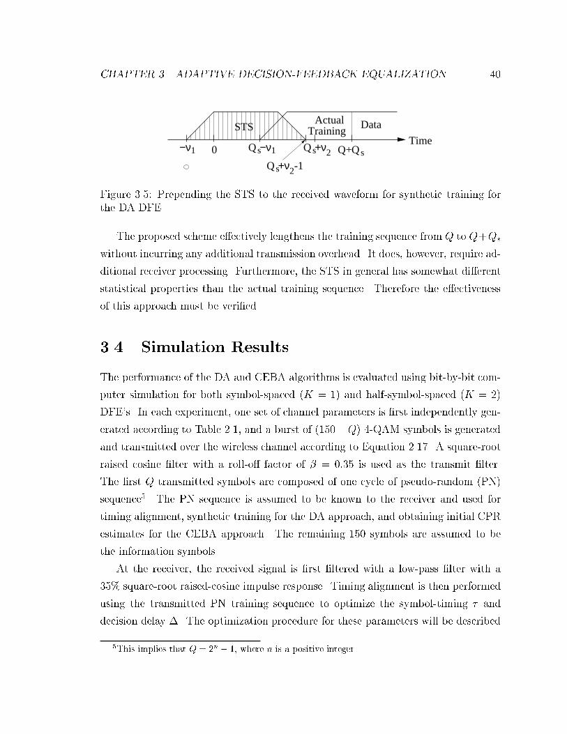
CHAPTER 3. ADAPTIVE DECISION-FEEDBACK EQUALIZATION 40
Qs Qs+ν2 Qs
Qs+ν2
����
����
−ν −ν1 10 Q+
ActualTraining
DataSTS
-1
Time
Figure 3.5: Prepending the STS to the received waveform for synthetic training for
the DA DFE.
The proposed scheme e�ectively lengthens the training sequence from Q to Q+Qs
without incurring any additional transmission overhead. It does, however, require ad-
ditional receiver processing. Furthermore, the STS in general has somewhat di�erent
statistical properties than the actual training sequence. Therefore the e�ectiveness
of this approach must be veri�ed.
3.4 Simulation Results
The performance of the DA and CEBA algorithms is evaluated using bit-by-bit com-
puter simulation for both symbol-spaced (K = 1) and half-symbol-spaced (K = 2)
DFE's. In each experiment, one set of channel parameters is �rst independently gen-
erated according to Table 2.1, and a burst of (150+Q) 4-QAM symbols is generated
and transmitted over the wireless channel according to Equation 2.17. A square-root
raised cosine �lter with a roll-o� factor of � = 0:35 is used as the transmit �lter.
The �rst Q transmitted symbols are composed of one cycle of pseudo-random (PN)
sequence5. The PN sequence is assumed to be known to the receiver and used for
timing alignment, synthetic training for the DA approach, and obtaining initial CPR
estimates for the CEBA approach. The remaining 150 symbols are assumed to be
the information symbols.
At the receiver, the received signal is �rst �ltered with a low-pass �lter with a
35% square-root raised-cosine impulse response. Timing alignment is then performed
using the transmitted PN training sequence to optimize the symbol-timing � and
decision delay �. The optimization procedure for these parameters will be described
5This implies that Q = 2n � 1, where n is a positive integer.
CHAPTER 3. ADAPTIVE DECISION-FEEDBACK EQUALIZATION 41
in detail in Chapter 4. Note that in this chapter, timing alignment is performed before
equalization starts, therefore the same optimization procedures for � and � are used
for both the CEBA and DA approaches. After the timing alignment parameters are
acquired, the DFE �lter coe�cients are adapted using the DA and CEBA approaches.
For the CEBA approach, the PN training sequence is used to obtaining initial CPR
estimates. During the remaining 150 symbols, the CPR estimates are updated once
per symbol period using the received signal and past decisions, and the DFE �lter
coe�cients are computed from the CPR estimates on a symbol-by-symbol basis as
described in Section 3.3.1. For the DA approach, the PN training is used to generate
a STS of length Qs. The STS is prepended to the received signal burst, and the DFE
�lter coe�cients are adapted once per symbol period using the signal samples and past
decisions as described in Section 3.3.2. For either approach, the number of decision
errors is tabulated for the 150 information symbols. The entire process is repeated
15,000 times. After that, it is continued until 3,000 bit errors are accumulated or
7,500,000 symbols are transmitted, whichever occurs �rst. In all experiments the
feedforward sections of the adaptive DFE span four symbol periods. The feedback
section has three taps spaced at the symbol period.6
3.4.1 Synthetic Training for DA DFE
Figure 3.6 shows the average bit-error rate (BER) for the symbol-spaced (K = 1) DA
DFE with synthetic training. The average BER is de�ned as the ratio of the number
of accumulated bit errors to the total number of transmitted bits. Here the channel
is assumed to have a Gaussian power-delay pro�le with a rms delay-spread of 50ns
and average delay of 200ns. In Figure 3.6, the average BER is shown as a function of
the normalized delay spread d, de�ned as
d =rms delay-spread
symbol period: (3.56)
6Though choices of DFE parameters were empirically chosen, they are tested using simulations
over a broad range of channel conditions.

CHAPTER 3. ADAPTIVE DECISION-FEEDBACK EQUALIZATION 42
10-1
10-3
10-2
Unequalized
0.5 0.75 1.0
Ave
rage
BE
R
Normalized Delay-Spread0.25
Q=15,Qs=3
Q=15,Qs=15
Q=15,Qs=7
Q=15,Qs=0
Q=31,Qs=0
Figure 3.6: The average BER of the symbol-spaced (K = 1) DA DFE with synthetic
training. The channel is assumed to have a Gaussian power-delay pro�le with a rms
delay-spread of 50 ns and average delay of 200 ns. The average SNR is 15 dB. Di�erent
training sequence lengths Q and STS lengths Qs are used.
For an rms delay-spread of 50ns and 4-QAM modulation, d = 0:25 and d = 1:0
correspond to data rates of 10 Mb/s and 40 Mb/s, respectively. The average SNR of
in this �gure is �xed at 15 dB. It is de�ned as the ratio of the signal power, averaged
over the Rayleigh distributed multipath fading, to the mean Gaussian noise power
at the output of the receive �lter (see Equations 2.17 and 2.18). For our simulation
setup the average SNR is numerically equal to the ratio of transmitted energy per bit
to the two-sided power spectral density of the AWGN. �1 = �2 = 3 (a total of 7 taps)
is used here for estimating the CPR for synthetic training purposes.
Di�erent combinations of actual training sequence length (Q) and STS length
(Qs) are tested. It can be seen from Figure 3.6 that without using STS (Qs = 0),
increasing the length of the actual training sequence from Q = 15 to Q = 31 results in
a 20% to 50% reduction in average BER. This is achieved at the price of both increased
transmission overhead and receiver processing. However, it can also be seen that with
Q �xed at 15, the DFE performance can be improved without introducing additional
transmission overhead by using a STS. The performance improves as the STS length
increases. In particular with (Q;Qs) = (15; 15) (a total of 30 \e�ective" training

CHAPTER 3. ADAPTIVE DECISION-FEEDBACK EQUALIZATION 43
symbols), the DFE performance is as good as using Q = 31 without STS. In other
words, STS is capable of achieving the same performance improvement as additional
actual training symbols without incurring any transmission overhead.
The performance of unequalized 4-QAM modulation is also plotted in Figure 3.6
as a baseline for comparison. It can be seen that without equalization, the BER
increases monotonically as d increases. This is expected because as d increases, the
ISI becomes more severe and reliable communications becomes more di�cult without
equalization. On the other hand, the average BER of the DFE decreases as d increases
from 0.25 to 0.5. As d increases beyond 0.5, the average BER increases with d. This
implies that as d increases from 0.25 to 0.5, the advantage of having more time
diversity outweighs the disadvantage of increased ISI. However, as d increases beyond
0.5, the length of the FIR DFE's becomes insu�cient and the increased residual ISI
degrades the performance. It can also be seen that the performance of the DFE is,
in general, signi�cantly superior to the unequalized case. At d = 1:0, for example,
the average BER of the DFE is lower than that of the unequalized case by almost an
order of magnitude.
The average BER of the symbol-spaced DFE is plotted in Figure 3.7 for di�erent
CPR estimate lengths. Here �1 and �2 are set to be equal and various di�erent
values are used. The channel is assumed to have a Gaussian power-delay pro�le with
normalized delay-spread d = 0:5, and the average SNR is set to 15 dB. The lengths
Q and Qs of the actual and synthetic training sequences, respectively, are both set
to 15. It can be seen that the average BER decreases only marginally as �1 and �2
increase beyond 3. There are two explanations for this observation. First, the number
of taps in the CPR estimate is limited by the length Q of the actual training sequence.
With Q �xed, the CPR estimate becomes increasing inaccurate as �1 and �2 increase.
Secondly, with a normalized delay-spread of 0.5, �1 = �2 = 3 is adequately long as
far as synthetic training is concerned. Increasing �1 and �2 beyond 3 does not make
the statistics of the STS any more reliable.
Similar plots for the half-symbol-spaced (K = 2) DFE are shown in Figures 3.8 and
3.9. The average BER's for various combinations of (Q;Qs) are shown in Figure 3.8 as
a function of d, while the average BER for various values of �1 and �2 (with �1 = �2)

CHAPTER 3. ADAPTIVE DECISION-FEEDBACK EQUALIZATION 44
10-1
10-3
10-2
Ave
rage
BE
R
ν 1 ( )ν 2
3 4 52
Figure 3.7: Average BER of the symbol-spaced (K = 1) DA DFE using various CPR
estimate lengths for synthetic training. �1 and �2 are both set to be equal to the value
of the abscissa. The channel has a Gaussian power-delay pro�le with a normalized
delay-spread of 0.5. The rms delay-spread and average delay are 50 ns and 200 ns,
respectively. The average SNR is 15 dB. Synthetic training with Q = Qs = 15 is
used.
10-1
10-3
10-2
Unequalized
0.5 0.75 1.0
Ave
rage
BE
R
Normalized Delay-Spread0.25
Q=15,Qs=3
Q=15,Qs=15
Q=15,Qs=7
Q=15,Qs=0
Q=31,Qs=0
Figure 3.8: The average BER of the half-symbol-spaced (K = 2) DA DFE with
synthetic training. The channel is assumed to have a Gaussian power-delay pro�le
with a rms delay-spread of 50 ns and average delay of 200 ns. The average SNR is 15
dB. Di�erent training sequence lengths Q and STS lengths Qs are used.

CHAPTER 3. ADAPTIVE DECISION-FEEDBACK EQUALIZATION 45
10-1
10-3
10-2
Ave
rage
BE
R
ν 1 ( )ν 2
3 4 52
Figure 3.9: Average BER of the half-symbol-spaced (K = 2) DA DFE using various
CPR estimate lengths for synthetic training. �1 and �2 are both set to be equal
to the value of the abscissa. The channel has a Gaussian power-delay pro�le with a
normalized delay-spread of 0.5. The rms delay-spread and average delay are 50 ns and
200 ns, respectively. The average SNR is 15 dB. Synthetic training with Q = Qs = 15
is used.
CHAPTER 3. ADAPTIVE DECISION-FEEDBACK EQUALIZATION 46
are shown in Figure 3.9. In all cases the channel is assumed to have a Gaussian
power-delay pro�le and the average SNR is set at 15 dB. We can see that the general
conclusions for the symbol-spaced (K = 1) case also hold in these plots.
3.4.2 Comparison of CEBA and DA DFE
Figure 3.10(a) shows the average bit-error rate (BER) for symbol-spaced (K = 1) and
half-symbol-spaced (K = 2) DA and CEBA DFE's. The average BER is shown as a
function of the average SNR. The channel is again assumed to have a Gaussian power-
delay pro�le with a normalized delay-spread of 0.5. Q = 15 PN symbols are used for
training. For the DA DFE, a STS with Qs = 15 symbols is used for synthetic training.
�1 = �2 = 3 is used for estimating the CPR for DA DFE synthetic training and CEBA
DFE �lter coe�cient adaptation. Only average SNR's greater than or equal to 10 dB
are simulated, because it had previously been found that the average BER's for lower
average SNR's are too high to be of interest to data communications[43]. It can be
seen that at d = 0:5, the di�erence between the average BER performance of symbol-
spaced DA and CEBA DFE's is insigni�cant. This is consistent with previously
reported results[44]. However, here we �nd that DA is slightly better than CEBA,
while it was found in [44, 45] that the reverse is true. The reason for this discrepancy is
that in this dissertation we did not assume knowledge of the exact number of channel
taps. In our simulations we generated the received signal in continuous time; while in
[44, 45] discrete-time equivalent channels with known �xed lengths are used to directly
generate the signal component of the received waveform samples. It can also be seen
that for d = 0:5, the di�erence between half-symbol-spaced (K = 2) and symbol-
spaced (K = 1) DA DFE's is also slight. This is because d = 0:5 is relatively small
for the DFE structure used here. When d is increased, the performance di�erence
between symbol-spaced and half-symbol-spaced DA DFE's becomes more signi�cant.
Finally, it can be seen that the CEBA DFE with K = 2 is signi�cantly worse than all
the other cases. In fact going from K = 1 to K = 2 incurs a signi�cant performance
loss for the CEBA DFE.
Figure 3.10(b) shows the average BER as a function of normalized delay-spread d
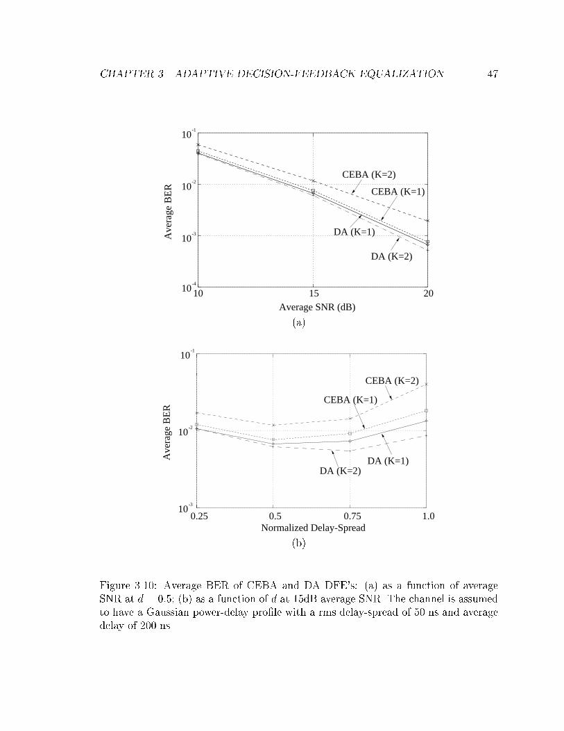
CHAPTER 3. ADAPTIVE DECISION-FEEDBACK EQUALIZATION 47
10 15 20Average SNR (dB)
10-1
10
10
10
-3
-4
-2
Ave
rage
BE
RCEBA (K=2)
CEBA (K=1)
DA (K=2)
DA (K=1)
(a)
10-1
10-3
10-2
0.25 0.5 0.75 1.0
DA (K=1)Ave
rage
BE
R
Normalized Delay-Spread
CEBA (K=2)
CEBA (K=1)
DA (K=2)
(b)
Figure 3.10: Average BER of CEBA and DA DFE's: (a) as a function of average
SNR at d = 0:5; (b) as a function of d at 15dB average SNR. The channel is assumed
to have a Gaussian power-delay pro�le with a rms delay-spread of 50 ns and average
delay of 200 ns.
CHAPTER 3. ADAPTIVE DECISION-FEEDBACK EQUALIZATION 48
at an average SNR of 15 dB. For the DA approach, it can be seen that as d increases
from 0.25 to 0.75, performance improvement of K = 2 (half-symbol-spaced) over
K = 1 (symbol-spaced) becomes increasingly signi�cant. This is because when d
is small, the channel is close to a at-fading channel, and relatively few taps are
required to handle the small amount of ISI. However, as d increases, the ISI caused
by multipath propagation becomes more severe, and more degrees of freedom in the
DFE are necessary.
For the CEBA approach, on the other hand, K = 2 is much worse than K = 1
for all d. This leads us to conclude that, for the argument for DA DFE's to hold
here, there must be another factor that seriously degrades the performance of K = 2
CEBA DFE. This factor is identi�ed in Section 3.5, where a remedial technique is
described.
It can also be seen that, for both K = 1 and K = 2, DA outperforms CEBA for
all cases simulated here, with larger performance gains at higher d. This is because
the CEBA DFE is more sensitive to variations in d than the DA DFE. CEBA is a
stochastic approach in which the second-order statistics of the signal are computed
using �xed-length CPR estimates. For small d, with high probability the actual
number of channel taps is smaller than or comparable to the number of estimated
CPR taps. The CPR estimates are therefore unbiased with high probability, and the
estimated second-order statistics are accurate for most channel realizations. However,
as d increases, the actual CPR becomes stochastically longer, therefore the CPR
estimates become biased because of insu�cient length, and the estimated second-order
statistics are inaccurate. For the CEBA approach, therefore, the increase of average
BER with d re ects both insu�cient CPR estimate length and insu�cient number
of taps in the DFE �lters to handle the ISI. The DA approach, on the other hand,
is a deterministic approach in which nothing is assumed about the statistics of the
signal. Therefore the performance degradation as d increases re ects only insu�cient
number of taps in the DFE �lters. We can thus conclude that the DA approach is
more robust than the CEBA approach with respect to delay-spread variations.

CHAPTER 3. ADAPTIVE DECISION-FEEDBACK EQUALIZATION 49
3.5 CEBA DFE with Regularization
In the previous section, the performance of the half-symbol-spaced CEBA DFE is
much worse than the symbol-spaced CEBA DFE. The performance loss of K = 2
over K = 1 is as large as 2 dB for the high-SNR case. To understand this behavior,
one should refer to the MMSE solution in Equations 3.48 and 3.49. It can be shown
that RP = PP� �HH� is singular if NfK > Nf + �1 + �2 �Nb: For our simulations
we have Nf = 4, Nb = 3 and �1 = �2 = 3. Therefore if K � 2, RP will be singular.
RN , on the other hand, is the autocorrelation matrix of the additive Gaussian noise
after sampling (see Equation 3.44). Since the impulse response of the receive �lter is
a truncated square-root raised-cosine pulse with symbol period T , the autocorrelation
function of the noise component at the output of the receive �lter (before sampling)
is approximately a raised-cosine pulse with symbol period T . Therefore, if only one
sample is taken per symbol period (K = 1), the sampled noise would be approximately
white, and RN is very close to diagonal. In this case RP + RN is likely to be
well-conditioned7, even when RP is singular. However, if the noise is over-sampled
(K > 1), the discrete-time power spectrum of the sampled noise will be very small in
the region(1+�)
K� < j!j < �, where � is the roll-o� factor of the receive �lter (� = 0:35
in our simulations) and ! is the discrete-time frequency. RN , as a consequence, will
be ill-conditioned[38], and RP +RN is likely to be ill-conditioned if RP is singular.
This leads to inaccuracies in solving for the DFE �lter coe�cients for the K = 2 case,
which in turn results in poor BER performance as we have observed in the previous
section.
To remedy the situation, we propose optimizing the fractionally-spaced CEBA
DFE using a \regularized" criterion[42, 46]. \Regularization" or \leakage"[47, 48, 49,
50, 51] is a technique that is used in the context of adaptive �ltering to improve the
stability of numerical algorithms. In this technique, the cost function is augmented by
a term which in some way bounds the energy in adaptive �lter response. The resulting
adaptive algorithms then try to �nd a compromise setting between minimizing the
7A matrix is ill-conditioned if the ratio of the maximum singular value to the minimum singular
value is much greater than 1. It should be kept in mind that here RP is a random matrix.
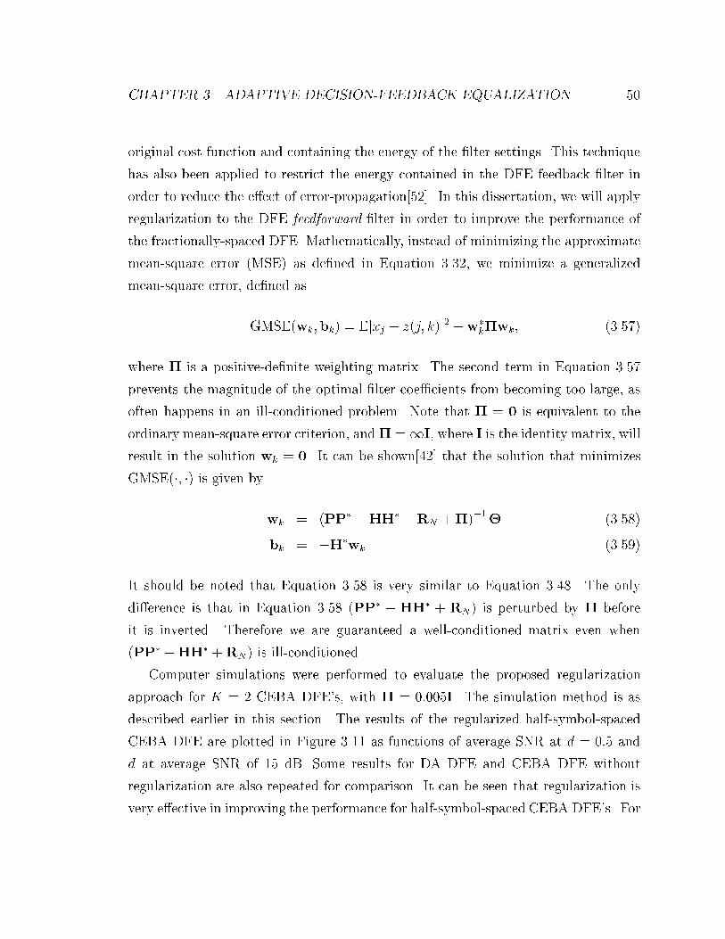
CHAPTER 3. ADAPTIVE DECISION-FEEDBACK EQUALIZATION 50
original cost function and containing the energy of the �lter settings. This technique
has also been applied to restrict the energy contained in the DFE feedback �lter in
order to reduce the e�ect of error-propagation[52]. In this dissertation, we will apply
regularization to the DFE feedforward �lter in order to improve the performance of
the fractionally-spaced DFE. Mathematically, instead of minimizing the approximate
mean-square error (MSE) as de�ned in Equation 3.32, we minimize a generalized
mean-square error, de�ned as
GMSE(wk;bk) = Ejxj � z(j; k)j2 +w�k�wk; (3.57)
where � is a positive-de�nite weighting matrix. The second term in Equation 3.57
prevents the magnitude of the optimal �lter coe�cients from becoming too large, as
often happens in an ill-conditioned problem. Note that � = 0 is equivalent to the
ordinary mean-square error criterion, and� =1I, where I is the identity matrix, will
result in the solution wk = 0. It can be shown[42] that the solution that minimizes
GMSE(�; �) is given by
wk = (PP� �HH� +RN +�)�1� (3.58)
bk = �H�wk (3.59)
It should be noted that Equation 3.58 is very similar to Equation 3.48. The only
di�erence is that in Equation 3.58 (PP� � HH� + RN) is perturbed by � before
it is inverted. Therefore we are guaranteed a well-conditioned matrix even when
(PP� �HH� +RN) is ill-conditioned.
Computer simulations were performed to evaluate the proposed regularization
approach for K = 2 CEBA DFE's, with � = 0:005I. The simulation method is as
described earlier in this section. The results of the regularized half-symbol-spaced
CEBA DFE are plotted in Figure 3.11 as functions of average SNR at d = 0:5 and
d at average SNR of 15 dB. Some results for DA DFE and CEBA DFE without
regularization are also repeated for comparison. It can be seen that regularization is
very e�ective in improving the performance for half-symbol-spaced CEBA DFE's. For

CHAPTER 3. ADAPTIVE DECISION-FEEDBACK EQUALIZATION 51
10-1
10-4
10-3
10-2
DA (K=2)
10 15 20
Ave
rage
BE
R
Average SNR (dB)
CEBA (K=2)
CEBA/REG (K=2)
CEBA (K=1)
(a)
10-1
10-3
10-2
Ave
rage
BE
R
0.25 0.5 0.75 1.0Normalized Delay-Spread
CEBA (K=2)
CEBA (K=1)CEBA/REG (K=2)
DA (K=2)
(b)
Figure 3.11: Average BER of the half-symbol-spaced (K = 2) CEBA DFE with
regularization: (a) as a function of average SNR at d = 0:5; (b) as a function of
d at 15dB average SNR. The average BER's CEBA without regularization and DA
with K = 2 are also shown. The channel is assumed to have a Gaussian power-delay
pro�le with a rms delay-spread of 50 ns and average delay of 200 ns.

CHAPTER 3. ADAPTIVE DECISION-FEEDBACK EQUALIZATION 52
example, with d = 0:5, at high average SNR regularization improves the performance
of the K = 2 CEBA DFE by 2 dB. Furthermore, the half-symbol-spaced (K = 2)
regularized CEBA DFE outperforms the symbol-spaced CEBA DFE for 0:25 � d �1:0. However, regularized CEBA remains sensitive to variations in d. As mentioned
previously, this is because �xed-length CPR estimates are used to synthesize the
regularized DFE coe�cients. When d is large the estimate is biased, resulting in
DFE �lter coe�cients that are signi�cantly inferior to the DA solution.
3.6 Summary
Inter-symbol interference (ISI), caused by delay spread in a multipath propagation
environment, is one of the limiting factors in high-speed wireless data transmission.
Adaptive equalization is a digital signal processing technique that can be used to
reduce the e�ect of ISI. Among the multitude of adaptive equalization techniques,
the decision-feedback equalizer (DFE) is an attractive candidate for indoor wireless
data communications.
Adaptive decision-feedback equalization using recursive least-squares (RLS) algo-
rithms can be classi�ed into channel-estimation-based adaptation (CEBA) and direct
adaptation (DA). In CEBA, the channel pulse response (CPR) is �rst estimated using
the RLS algorithm, and the DFE coe�cients are computed as functions of the CPR
estimates. In DA, the DFE �lter coe�cients are directly computed from the received
signal samples using the RLS algorithm. In both cases a training sequence is required
to obtain reasonable initial values for the DFE �lter coe�cients. For the DA DFE,
we propose and analyze a synthetic training technique which e�ectively lengthens
the training sequence without incurring any additional transmission overhead. Sim-
ulation results show that this technique can work as good as lengthening the actual
training sequence if the sequence is long enough for the channel delay encountered.
In this dissertation, we have found that 1) DA slightly outperforms CEBA for
symbol-spaced DFE's when the amount of channel delay-spread is moderate; 2)
DA signi�cantly outperforms CEBA for fractionally-spaced cases regardless of delay-
spread; and 3) CEBA is more sensitive to the variations in delay-spread, therefore

CHAPTER 3. ADAPTIVE DECISION-FEEDBACK EQUALIZATION 53
both symbol-spaced and fractionally-spaced CEBA DFE's become signi�cantly infe-
rior to the DA DFE as the delay-spread is increased. These results are not entirely
consistent with previously reported results[44, 45]. The reason for the discrepancy
is that, to make our simulations realistic, we did not assume the knowledge of the
actual length of the channel. Therefore when the delay-spread is large for a random
realization of a channel, the CPR estimates used in the CEBA approach are biased,
resulting in poor performance.
We have also found that for fractionally-spaced CEBA DFE's, not only are the
CPR estimates biased, the minimummean-square error (MSE) solution (Equation 3.48)
is also ill-conditioned. To remedy that, we can use a regularization, or leakage, tech-
nique which minimizes a generalized MSE, as described in Equations 3.57, 3.58, and
3.59. Simulation results show that this technique is very e�ective. In particular, a gain
as much as 2dB in average SNR can be achieved by regularization. However, CEBA
with regularization remains more sensitive to variations in delay-spread than the DA
approach. The DA approach is therefore more robust with respect to delay-spread
variations.

Chapter 4
DFE Timing Alignment
It was shown in Chapter 3 that adaptive decision-feedback equalization is an e�ective
technique to use against the impairment of ISI. However, in applying decision-feedback
equalization, the received signal must �rst be sampled at the \best" sampling instants
with respect to the received symbols. If a �nite impulse response (FIR) DFE is used,
as in this dissertation, then a decision delay must also be determined. While the
choice of sampling instants and decision delay is not crucial for equalizers with many
taps, the performance of FIR DFE's with small number of taps is sensitive to the
choice of these parameters[36]. We refer to the optimization of sampling instants and
DFE decision delay as the \timing alignment" problem.
A block diagram of an adaptive DFE is shown in Figure 4.1. As mentioned
previously, the �ltered received signal y(t) is sampled at a rate of K samples per
Tap-Wt.Adapt
xj
+FeedforwardFilter
FeedbackFilterDFE
zj∆y
j+y
j
AlignmentTiming
FilterReceiver r(t)
τ ∆Advance
Sample∆y(t)
Figure 4.1: Block diagram of an adaptive decision-feedback equalizer.
54
CHAPTER 4. DFE TIMING ALIGNMENT 55
symbol-period, where K is assumed to be an integer. The sampling period is therefore
Ts =T
K; (4.1)
where T is the symbol-period. We can denote these samples as
rj = y(jTs + �); j = 0; 1; : : : ; (4.2)
where � is the sampling instant, or symbol-timing, parameter. It is the time at which
the �rst sample is taken. Note that rj in Equation 4.2 and yj;k in Equation 3.17
describe the same discrete-time signal using di�erent indexing schemes. In particular,
we have
yj;k = rK(j+1)�k�1; (4.3)
for j = 0; 1; : : : and k = 0; 1; : : : ; (K � 1). The adaptive DFE then uses the linear
combination of the components of the signal samples yj+�;yj+��1; : : : ;yj+��Nf+1,
de�ned in Equation 3.22, and past decisions x̂j�1; x̂j�2; : : : ; x̂j�Nbto estimate the
transmitted symbol xj. The integer � is the \decision delay" of the DFE[29, 35, 36,
37]. The timing alignment problem, then, refers to the optimization of the parameters
� and �.
4.1 Sampling Instant Optimization
As mentioned previously, Ts-spaced samples of the �ltered received signal y(t) are fed
into the equalizer, where Ts is the tap-spacing of the feedforward sections of the DFE.
The sampling instant � , de�ned in Equation 4.2, re ects the delay introduced by the
channel as well as the band-edge behavior of the frequency spectrum of rj when there
is aliasing, and must be chosen carefully in order to achieve acceptable bit error rate
(BER) performance.
In our approach the sampling instant is acquired by �rst over-sampling y(t). �
is next optimized in two steps. In the �rst step a coarse value t0 is obtained based
on the correlation in time between the sampled received signal and the transmitted

CHAPTER 4. DFE TIMING ALIGNMENT 56
training sequence. This value re ects the average delay introduced by the multipath
propagation channel, and thus will be referred to as the \sampling delay." A �ne-
tuning adjustment �0, where 0 � �0 < Ts, is next determined based on frequency-
domain calculations. This value controls the band-edge behavior of the sampled
received signal, and will be referred to as the \sampling phase." The resulting value
for � is then
� = t0 + �0: (4.4)
Mathematically, let
~rl = y
�lTs
L
�; l = 0; 1; : : : ; (4.5)
be the over-samples of the received signal, where L is the over-sampling factor for
timing alignment. The complex time correlations �m between the transmitted train-
ing sequence and the received signal are then calculated at M -over-sample shifts.
Speci�cally, we have
�m =Q�1Xj=0
x�j~rmM+jL; m = 0; 1; : : : ; dLt0;max
MTse; (4.6)
where Q is the length of the training sequence, M is the resolution in over-samples
to which t0 is estimated, and t0;max is the maximum channel delay expected1. The
resulting value for the sampling delay then corresponds to the position, accurate to
MTs
L, of the correlation peak between the received signal and transmitted training
sequence, i.e.
t0 = m0
MTs
L; (4.7)
where
m0 = argmax fj�mjg : (4.8)
Given t0, the sampling phase is obtained based on frequency-domain calculations.
Let p̂(l)k
denote the Ts-spaced channel pulse response (CPR) estimate corresponding
1In this dissertation we assume that the presence of a data burst is detected with 100% accuracy.
Only the delay introduced by the channel and the appropriate sampling phase remain to be found.
The data burst can be detected by, for example, comparing the correlation peak to a preset threshold.

CHAPTER 4. DFE TIMING ALIGNMENT 57
to sampling delay m0(MTs
L) and sampling phase l(Ts
L), i.e. an estimate of the CPR
de�ned as
p(l)k= p(kTs +m0
MTs
L+ l
Ts
L); k = : : : ;�1; 0; 1; : : : ; (4.9)
where p(t) is de�ned in Equation 3.12. Furthermore, let P̂ (l)(!) denote the discrete-
time Fourier transform of p̂(l)k. Finally, de�ne the quantity SER(l)
1 as
SER(l)1 =
Z 2�
0ln
�N0
2+���P̂ (l)(!)
���2� d!; l = 0; 1; : : : ; (L� 1): (4.10)
The estimated sampling phase then corresponds to the candidate phase with the
highest SER(l)1 , i.e.
�0 = l0Ts
L; (4.11)
where
l0 = argmaxnSER(l)
1
o: (4.12)
The reason for using the metric in Equation 4.10 for sampling phase optimization
is that it is proportional to the logarithm of the maximum output signal-to-MSE
ratio (SER) achievable by a DFE with an in�nite number of taps in the feedforward
and feedback sections[34]. If a particular value of the sampling phase results in poor
performance for an in�nite-length DFE, the performance of a FIR DFE will very
likely be even worse. Therefore, using SER(l)1 can, in principle, preclude the sampling
phases that are likely to result in poor performance.
It should be noted that �rst, the CPR estimate p̂(l)k
can be obtained using least-
squares methods[38]. Furthermore, as described in Chapter 3, a �xed-length CPR
estimate fp̂t;��1 � t � �2g is used. Secondly, the frequency-domain spectra P̂ (l)(!)
can be obtained from p̂(l)kusing the fast Fourier transform (FFT). The spectra P̂ (l)(!)
di�er from each other only in the region where aliasing occurs. Therefore when 1Ts
is
greater than twice the highest frequency component of the received signal spectrum,
SER(l)1 will be equal for all l and �0 cannot be obtained using the proposed method.
This typically happens for a fractionally-spaced DFE (K > 1) where the feedforward
�lter is spaced at less than a symbol period. However, our simulation results show

CHAPTER 4. DFE TIMING ALIGNMENT 58
that in this case sampling phase has an insigni�cant e�ect on the average BER per-
formance. Therefore if a fractionally-spaced DFE is used, only the sampling delay
t0 needs to be optimized. �0 can be set to an arbitrary value after t0 is obtained.
This is because for fractionally-spaced DFE's, the �ltered received signal is sampled
at a frequency higher than the Nyquist rate. Therefore there is no aliasing and the
spectrum of the sampled signal behaves the same in the band-edge, regardless of the
value of �0. Thirdly, for the case when 1Ts
is less than twice the highest frequency
component of the received signal spectrum, the integration in Equation 4.10 needs
to be carried out only over the region where aliasing occurs. This property could
be exploited to reduce the number of mathematical operations required to evalu-
ate SER(l)1 . For example, for square-root raised-cosine spectral shaping with roll-o�
factor � and symbol-spaced DFE, the integration needs to be carried out only for
! 2 [(1� �)�; (1 + �)�]. Finally, instead of computing p̂(l) for every l, we could �rst
estimate the unaliased channel frequency response P̂ (!). The spectra P̂ (l)(!) can
then be obtained by aliasing P (!).
4.2 Decision-Delay Optimization
The performance of the adaptive DFE is very sensitive to the choice of the decision
delay �, especially when number of taps in the feedforward �lter is small. � re ects
the signal spread introduced by multipath propagation and controls the trade-o�
between time diversity and ISI. In general � can be optimized in an a priori or a
posteriori fashion.
4.2.1 A Priori Optimization
Conventionally the value of the decision delay for a DFE is determined in an a priori
manner, i.e. before the DFE operation starts, based on statistical computations. The
optimization metric is usually a function of the CPR estimates. After the decision de-
lay is chosen, the DFE �lter coe�cients can be adaptively computed using algorithms
described in Chapter 3, and the data burst can be decoded. Several researches have

CHAPTER 4. DFE TIMING ALIGNMENT 59
been devoted to e�ciently optimizing the decision delay[29, 35, 37, 53]. One natural
approach is to choose the decision delay that corresponds to the highest SER at the
output of the DFE. The output SER of a DFE is given by
SERDFE(�) =1
MSEmin;k
; (4.13)
where MSEmin;k is given by Equation 3.52. Note that MSEmin;k is implicitly a function
of �. Furthermore, computation of SERDFE(�) requires inverting a Nf�Nf complex
matrix. Al-Dhahir and Cio�[37] developed a fast algorithm for computing MSEmin;k
which can be used to e�ciently optimize �.
SERDFE(�) is the optimal (in the MMSE sense) metric to use if the CPR is known
exactly at the receiver. However, since only an estimate of the CPR is available for
computing SERDFE(�), the decision delay thus obtained is optimal only to within the
accuracy of the CPR estimates. In this case, an approximate, yet computationally
simpler, ad hoc criterion may su�ce to yield a decision delay that corresponds to
a near-optimal BER performance. One such ad hoc optimization metric that we
propose and analyze in this dissertation is the output SER achievable by a FIR
linear equalizer[33] with Nf taps and decision delay �. The tap-weights of this linear
equalizer are set so that they match the CPR within the span of the equalizer. This
metric, denoted as SERLE(�), is de�ned as
SERLE(�) =
���PNf�1m=0 kp̂��mk2
���2P�2
s=��1s6=�
���PNf�1m=0 p̂
���mp̂s�m
���2 +PNf�1s=0
PNf�1m=0 p̂
���mRm�sp̂��s
; (4.14)
where
Rm�s = E [nsn�m] (4.15)
is the noise correlation matrix. For a given channel, Nf and �, it can be shown that
SERLE(�) � SERDFE(�), hence SERLE(�) is in fact a lower bound of SERDFE(�).
Since no matrix inversion is involved, SERLE(�) is easier to compute than SERDFE(�),
especially when the noise is white and the length of the CPR estimate is long. As will
be shown by computer simulation, the two metrics can achieve comparable average

CHAPTER 4. DFE TIMING ALIGNMENT 60
BER performance.
4.2.2 A Posteriori Optimization
A priori optimization of the decision delay based on CPR estimates is suitable for
continuous data transmission over a relatively static channel. For bursty mobile com-
munication applications such as a time division multiple access (TDMA) based indoor
wireless data network, data are transmitted in short blocks. Because of the mobile
nature of wireless communications, the communication channel may be di�erent from
block to block. In this case the \optimal" decision delay that minimizes the over-
all average BER is not only channel-dependent but also data-dependent. Therefore,
for short-burst wireless communications it may be necessary to actually decode the
transmitted data burst using several di�erent decision delays, and choose the \best"
output. This is the a posteriori approach for decision delay optimization. One possi-
ble brute-force a posteriori approach is to store the samples of the received signal and
perform multiple equalization operations using all reasonable values for �. Cyclic
redundancy coding (CRC) checksums could be used to detect errors and the one with
the smallest number of errors is chosen as the �nal output. Although apparently
this approach will yield the \optimal" average BER performance, the computational
cost associated with multiple equalizations will be undesirably high. Furthermore,
this approach relies on the CRC checksum to determine an optimal choice �. This
may require a powerful code and, as a result, incur more transmission overhead. An
e�cient way to reduce the complexity and transmission overhead of the a posteriori
optimization approach while maintaining a low average BER remains to be investi-
gated. The discussion of such techniques is deferred until Chapter 7.
4.3 Simulation Results
The performance of the timing alignment algorithms presented in this chapter is
evaluated using bit-by-bit computer simulation for both K = 1 (symbol-spaced) and
K = 2 (half-symbol-spaced) DA DFE's. In each experiment, one set of channel
CHAPTER 4. DFE TIMING ALIGNMENT 61
parameters is �rst generated according to the distributions tabulated in Table 2.1.
A burst of 165 4-QAM symbols is next generated and transmitted over the wireless
channel according to Equation 2.17. A square-root raised cosine �lter with a roll-
o� factor of � = 0:35 is used both as the transmit and receive �lters. The �rst 15
transmitted symbols are composed of one cycle of pseudo-random (PN) sequence.
They are assumed to be known to the receiver, and are used for timing alignment as
well as synthetic training to initialize the adaptive DFE. The CPR estimate used for
timing alignment and synthetic training have parameters �1 = �2 = 3. A synthetic
training sequence (STS) with 15 symbols is used for synthetic training as described
in Chapter 3. During the 150 information symbols, the coe�cients of the DA DFE
are updated using the received signal and past decisions, as described previously in
Chapter 3. The number of decision errors is tabulated for these 150 symbols. The
entire process is repeated 15,000 times. After that, it is continued until 3,000 bit
errors are accumulated or 7,500,000 symbols are transmitted, whichever occurs �rst.
As in Chapter 3, in all experiments the feedforward sections of the adaptive DFE
span four symbol periods. The feedback section has three taps spaced at the symbol
period.
4.3.1 Sampling Instant Optimization
The average BER's of the symbol-spaced (K = 1) DA DFE are shown in Figure 4.2 as
functions of the normalized delay-spread, de�ned in Equation 3.56. As in Chapter 3,
the average BER is de�ned as the ratio of the number of accumulated bit errors
to the total number of transmitted bits. Here the channel is assumed to have a
Gaussian power-delay pro�le with a rms delay-spread of 50 ns and average delay of
200 ns. The average SNR is �xed at 15 dB in this �gure. It is de�ned as the ratio
of the signal power, averaged over the Rayleigh distributed multipath fading, to the
mean Gaussian noise power at the output of the receive �lter (see Equations 2.17 and
2.18). For our simulation setup the average SNR is numerically equal to the ratio
of transmitted energy per bit to the two-sided power spectral density of the AWGN.
An over-sampling factor of L = 16 is used, and the decision delay is optimized using
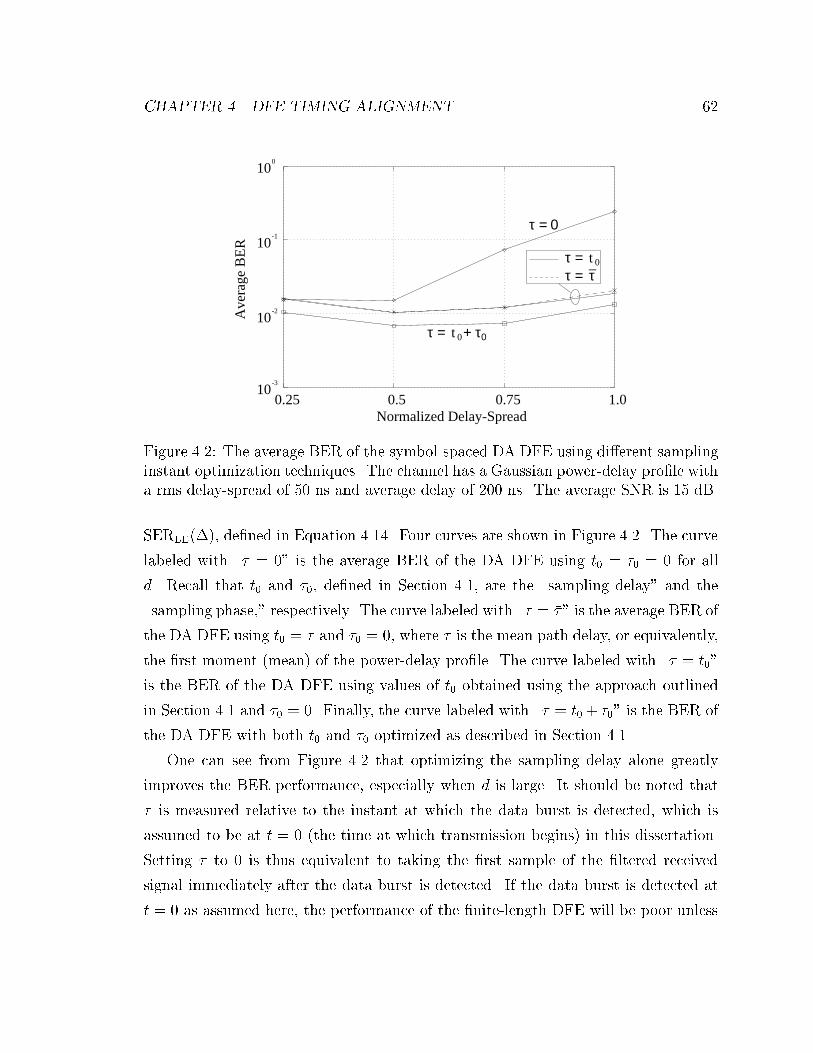
CHAPTER 4. DFE TIMING ALIGNMENT 62
10-3
10-2
10-1
100
τ0t 0τ = +
0tτ =
0.25 0.5 0.75 1.0
Ave
rage
BE
R
Normalized Delay-Spread
τ = 0
τ = τ _
Figure 4.2: The average BER of the symbol-spaced DA DFE using di�erent sampling
instant optimization techniques. The channel has a Gaussian power-delay pro�le with
a rms delay-spread of 50 ns and average delay of 200 ns. The average SNR is 15 dB.
SERLE(�), de�ned in Equation 4.14. Four curves are shown in Figure 4.2. The curve
labeled with \� = 0" is the average BER of the DA DFE using t0 = �0 = 0 for all
d. Recall that t0 and �0, de�ned in Section 4.1, are the \sampling delay" and the
\sampling phase," respectively. The curve labeled with \� = ��" is the average BER of
the DA DFE using t0 = �� and �0 = 0, where �� is the mean path delay, or equivalently,
the �rst moment (mean) of the power-delay pro�le. The curve labeled with \� = t0"
is the BER of the DA DFE using values of t0 obtained using the approach outlined
in Section 4.1 and �0 = 0. Finally, the curve labeled with \� = t0+ �0" is the BER of
the DA DFE with both t0 and �0 optimized as described in Section 4.1.
One can see from Figure 4.2 that optimizing the sampling delay alone greatly
improves the BER performance, especially when d is large. It should be noted that
� is measured relative to the instant at which the data burst is detected, which is
assumed to be at t = 0 (the time at which transmission begins) in this dissertation.
Setting � to 0 is thus equivalent to taking the �rst sample of the �ltered received
signal immediately after the data burst is detected. If the data burst is detected at
t = 0 as assumed here, the performance of the �nite-length DFE will be poor unless
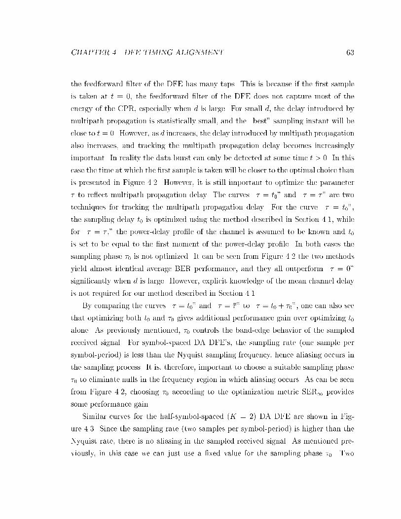
CHAPTER 4. DFE TIMING ALIGNMENT 63
the feedforward �lter of the DFE has many taps. This is because if the �rst sample
is taken at t = 0, the feedforward �lter of the DFE does not capture most of the
energy of the CPR, especially when d is large. For small d, the delay introduced by
multipath propagation is statistically small, and the \best" sampling instant will be
close to t = 0. However, as d increases, the delay introduced by multipath propagation
also increases, and tracking the multipath propagation delay becomes increasingly
important. In reality the data burst can only be detected at some time t > 0. In this
case the time at which the �rst sample is taken will be closer to the optimal choice than
is presented in Figure 4.2. However, it is still important to optimize the parameter
� to re ect multipath propagation delay. The curves \� = t0" and \� = ��" are two
techniques for tracking the multipath propagation delay. For the curve \� = t0",
the sampling delay t0 is optimized using the method described in Section 4.1, while
for \� = �� ," the power-delay pro�le of the channel is assumed to be known and t0
is set to be equal to the �rst moment of the power-delay pro�le. In both cases the
sampling phase �0 is not optimized. It can be seen from Figure 4.2 the two methods
yield almost identical average BER performance, and they all outperform \� = 0"
signi�cantly when d is large. However, explicit knowledge of the mean channel delay
is not required for our method described in Section 4.1.
By comparing the curves \� = t0" and \� = ��" to \� = t0 + �0", one can also see
that optimizing both t0 and �0 gives additional performance gain over optimizing t0
alone. As previously mentioned, �0 controls the band-edge behavior of the sampled
received signal. For symbol-spaced DA DFE's, the sampling rate (one sample per
symbol-period) is less than the Nyquist sampling frequency, hence aliasing occurs in
the sampling process. It is, therefore, important to choose a suitable sampling phase
�0 to eliminate nulls in the frequency region in which aliasing occurs. As can be seen
from Figure 4.2, choosing �0 according to the optimization metric SER1 provides
some performance gain.
Similar curves for the half-symbol-spaced (K = 2) DA DFE are shown in Fig-
ure 4.3. Since the sampling rate (two samples per symbol-period) is higher than the
Nyquist rate, there is no aliasing in the sampled received signal. As mentioned pre-
viously, in this case we can just use a �xed value for the sampling phase �0. Two

CHAPTER 4. DFE TIMING ALIGNMENT 64
10-3
10-2
10-1
100
Ave
rage
BE
R
0tτ = +0.5Ts
0tτ =
0.25 0.5 0.75 1.0Normalized Delay-Spread
τ = 0
Figure 4.3: The average BER of the half-symbol-spaced DA DFE using di�erent
sampling instant optimization techniques. The channel has a Gaussian power-delay
pro�le with a rms delay-spread of 50 ns and average delay-spread of 200 ns. The
average SNR is 15 dB.
such values are shown in Figure 4.3: �0 = 0 and �0 = 0:5Ts, where Ts is the sam-
pling period. It can be seen that these two values yield the same BER performance.
Furthermore, as in the symbol-spaced case, optimizing t0 alone results in a signi�-
cant performance gain. This can be explained using the same argument as presented
earlier in this section.
4.3.2 Decision Delay Optimization
The performance of the decision delay optimization approaches is also evaluated using
computer simulation. The channel is again assumed to have a Gaussian power-delay
pro�le with a rms delay-spread of 50 ns and average delay of 200 ns. For each burst,
� = t0+�0 is optimized as described in Section 4.1 using an over-sampling factor of L =
16. For the a priori optimization approach, SERDFE(�) de�ned in Equation 4.13 and
SERLE(�) de�ned in Equation 4.14 are simulated. For the a posteriori optimization
approach, multiple decision-feedback equalizations are performed using all possible
values of decision delay to yield multiple decoded bursts. The burst with the smallest

CHAPTER 4. DFE TIMING ALIGNMENT 65
DFE/SER LE
10-1
10-4
10-3
10-2
DFE/SER DFE
Ave
rage
BE
RIDEAL
FIXED
Average SNR2010 15
Figure 4.4: Average BER as a function of average SNR for di�erent decision delay
optimization schemes, �xed delay and ideal cases. The channel has a Gaussian power-
delay pro�le with normalized delay-spread d = 0:5. Symbol-spaced DA DFE's are
used.
number of bit errors is then used as the �nal output to tabulate the average BER. Note
that this scheme is not realizable because it requires the knowledge of the transmitted
data symbols at the receiver. A �xed-decision-delay case in which � = 2 is also
simulated to provide a baseline for comparison.
Figure 4.4 shows the average BER for the various decision-delay optimization
schemes as a function of the average SNR with d = 0:5. The curve labeled as \IDEAL"
corresponds to the BER of the unrealizable, a posteriori approach. It can be seen
that at d = 0:5 with average SNR greater than 10dB, SERDFE(�) always outperforms
SERLE(�) as a criterion for decision delay optimization. This shows that with a
50% normalized delay-spread, a 7-tap CPR estimate is adequately accurate as far
as decision delay optimization is concerned. The gap between the two curves is
insigni�cant for low average SNR and approximately 2dB for high average SNR. This
is because for low average SNR the performance is primarily noise-limited and for
high average SNR the performance is primarily ISI-limited. Since the decision delay
controls the trade-o� between time-diversity and ISI, it is more important when the
performance is ISI-limited. It can also be seen that both criteria greatly outperform

CHAPTER 4. DFE TIMING ALIGNMENT 66
0.25 0.5 0.75 1.0
10-1
10-2
10-3
010
SER LE
DFESER
Normalized Delay-Spread
Ave
rage
BE
RFIXED
IDEAL
Figure 4.5: Average BER as a function of normalized delay-spread for di�erent de-
cision delay optimization schemes, �xed delay and ideal cases. The channel has a
Gaussian power-delay pro�le with an average SNR of 15 dB. Symbol-spaced DA
DFE's are used.
the �xed case in which no decision delay optimization is performed, and that both are
signi�cantly inferior to the ideal case in which the number of bit errors is minimized
for each data burst. The latter observation can be explained as follows. For the a
priori decision delay optimization approach, the decision delay is optimized based
on an estimate of the channel before the transmitted data is decoded. However, for
short-burst transmissions the optimal value for decision delay is not only dependent
on the channel, but also dependent on the data burst itself. Therefore an a posteriori
approach such as the ideal case would outperform the a priori approach in terms of
average BER because by actually decoding the data the burst-dependence property
of optimal decision delay is taken into account.
The average BER's of the decision delay optimization approaches are shown in
Figure 4.5 as functions of d with the average SNR �xed at 15 dB. It can be seen
that for all but the �xed decision delay case, the average BER �rst decreases then
increases as d is increased from 0.25. While this phenomenon had been observed
in previous research[54] and Chapter 3 of this dissertation, here we �nd that this
is true only when the trade-o� between time diversity and ISI is handled properly
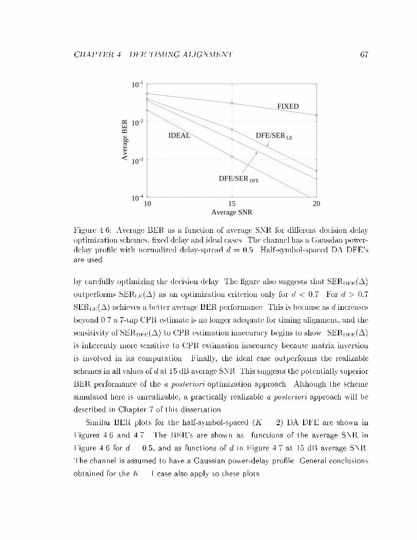
CHAPTER 4. DFE TIMING ALIGNMENT 67
10-1
10-4
10-3
10-2
DFE/SER DFE
DFE/SER LE
Ave
rage
BE
R
IDEAL
FIXED
Average SNR2010 15
Figure 4.6: Average BER as a function of average SNR for di�erent decision delay
optimization schemes, �xed delay and ideal cases. The channel has a Gaussian power-
delay pro�le with normalized delay-spread d = 0:5. Half-symbol-spaced DA DFE's
are used.
by carefully optimizing the decision delay. The �gure also suggests that SERDFE(�)
outperforms SERLE(�) as an optimization criterion only for d < 0:7. For d > 0:7
SERLE(�) achieves a better average BER performance. This is because as d increases
beyond 0.7 a 7-tap CPR estimate is no longer adequate for timing alignment, and the
sensitivity of SERDFE(�) to CPR estimation inaccuracy begins to show. SERDFE(�)
is inherently more sensitive to CPR estimation inaccuracy because matrix inversion
is involved in its computation. Finally, the ideal case outperforms the realizable
schemes in all values of d at 15 dB average SNR. This suggests the potentially superior
BER performance of the a posteriori optimization approach. Although the scheme
simulated here is unrealizable, a practically realizable a posteriori approach will be
described in Chapter 7 of this dissertation.
Similar BER plots for the half-symbol-spaced (K = 2) DA DFE are shown in
Figures 4.6 and 4.7. The BER's are shown as functions of the average SNR in
Figure 4.6 for d = 0:5, and as functions of d in Figure 4.7 at 15 dB average SNR.
The channel is assumed to have a Gaussian power-delay pro�le. General conclusions
obtained for the K = 1 case also apply to these plots.

CHAPTER 4. DFE TIMING ALIGNMENT 68
0.25 0.5 0.75 1.0
010
10-1
10-2
10-3
10-4
SER LE
DFESER
Normalized Delay-Spread
Ave
rage
BE
R
IDEAL
FIXED
Figure 4.7: Average BER as a function of normalized delay-spread for di�erent de-
cision delay optimization schemes, �xed delay and ideal cases. The channel has a
Gaussian power-delay pro�le with an average SNR of 15 dB. Half-symbol-spaced DA
DFE's are used.
4.4 Summary
Timing alignment refers to the optimization of sampling instants, or symbol-timing,
and DFE decision-delay. This process can be regarded as a procedure to \align"
the DFE with the channel pulse response. In this dissertation, timing alignment is
performed through channel estimation. The sampling instant, � , is �rst optimized in
two steps. In the �rst step, a coarse value t0 is obtained based on the correlation in
time between the sampled receive signal and the transmitted training sequence. This
value re ects the average delay introduced by the multipath propagation channel,
and is referred to as the \sampling delay." A �ne-tuning adjustment �0 is next
determined based on frequency-domain calculations. This value controls the band-
edge behavior of the sampled received signal and is referred to as the \sampling
phase." The resulting value for � is then t0 + �0.
After � is acquired, the decision delay � is next optimized. � controls the trade-
o� between time-diversity and ISI. It can be optimized in an a priori or a posteriori
fashion. For a priori optimization, the value of the decision delay for a DFE is

CHAPTER 4. DFE TIMING ALIGNMENT 69
determined based on statistical computations before the DFE operation starts. After
the decision delay is chosen, the DFE �lter coe�cients can be adaptively computed
using algorithms described in Chapter 3, and the data burst can be decoded. Two
metrics can be used for a priori optimization: SERDFE(�), de�ned in Equation 4.13,
and SERLE(�), de�ned in Equation 4.14. SERDFE(�) is approximately the maximum
SER at the output of a DFE with decision delay �. This quantity can be computed
using e�cient algorithms such as that developed by Al-Dhahir and Cio�[37]. It is the
optimal (in the MMSE sense) metric to use if the CPR is known exactly at the receiver.
However, since only an estimate of the CPR is available for computing SERDFE(�),
the decision delay thus obtained is optimal only to the within the accuracy of the
CPR estimates. In this case, an approximate, yet computationally simpler, ad hoc
metric may su�ce to yield a decision delay that corresponds to a near-optimal BER
performance. SERLE(�) is one such ad hoc metric. It is approximately the output
SER achievable by a FIR linear equalizer with decision delay � and Nf taps matched
to the CPR within the span of the equalizer.
For a posteriori optimization, the data burst is decoded using several di�erent
decision delays, and the \best" output is chosen. This yields better average BER per-
formance for short-burst transmissions over wireless channels where the average BER
is not only channel-dependent but also data-dependent. However, the computational
complexity associated with multiple equalizations is undesirably high. Furthermore, a
mechanism is required to determine which decoded output contains the fewest errors.
A selection mechanism, as well as an e�cient way to reduce computational complex-
ity while maintaining superior performance, are therefore desirable. The discussion
of such techniques is deferred until Chapter 7.
Simulation results show that it is very important to optimize the sampling delay
t0 in order to compensate for the delay introduced by multipath propagation. If a
symbol-spaced DFE is used, optimizing the sampling phase �0 can achieve signi�cant
additional performance gain. Furthermore, it is also very important to optimize the
decision delay �. It is shown by simulation that for a priori optimization, SERDFE(�)
provides better performance for smaller values of the normalized delay-spread d. On
the other hand, SERLE(�) is a better metric to use for larger d. However, the

CHAPTER 4. DFE TIMING ALIGNMENT 70
di�erence between these two approaches is small (within 1 dB for d = 0:5), therefore
the relative simplicity of SERLE(�) justi�es its use even when d is small. Finally,
it is also observed that the unrealizable, \ideal" a posteriori approach simulated
here outperforms all a priori approaches. This provides the incentive for further
investigation, as will be presented in Chapter 7.
Chapter 5
Receiver Diversity
Adaptive DFE has been shown in Chapter 3 to be an e�ective technique to use
against performance degradation due to inter-symbol interference (ISI). However,
when the SNR of a particular realization of the channel is low, the performance of
the adaptive DFE will be severely impaired by the additive white Gaussian noise
(AWGN). Therefore, when the channel delay-spread is moderate so that the adaptive
DFE is capable of suppressing the ISI with high probability, most transmission errors
are due to signal fading. Unfortunately the adaptive DFE is not capable of mitigating
signal fading, therefore for channels with moderate delay-spread, the performance of
the adaptive DFE is ultimately AWGN- and fading-limited.
Diversity, on the other hand, is a technique commonly used in wireless communi-
cation systems to combat signal fading in a at-fading environment[1]. It uses more
than one radio transmission channel to convey the same message in order to reduce
the e�ect of multipath propagation. The di�erent channels are referred to as diversity
branches. If several replicas of the information-carrying signal are received over mul-
tiple channels that have independent propagation parameters, then there is a good
likelihood that at least one of these received signals will not be in a fade at any given
time instant, thus making it possible to deliver adequate signal level to the receiver.
Diversity can greatly reduce the transmitter power required to achieve a certain per-
formance, because without diversity, the transmitter has to deliver a high power level
to protect the radio link against channel realizations with very low SNR's.
71
CHAPTER 5. RECEIVER DIVERSITY 72
There are many di�erent techniques[55, 57] for providing diversity branches with
independent channel statistics. For example, diversity can be achieved using multiple
receiver antennas separated in space (space diversity), having di�erent polarizations
(polarization diversity), or with di�erent beam angles (angle diversity). These tech-
niques are collective known as \antenna diversity" or \receiver diversity." They do
not require additional frequency spectrum resource. For space diversity, the receiver
antennas are separated by a suitable distance so that the corresponding diversity
channels are su�ciently decorrelated. The spacing required to obtain decorrelation
depends on the multipath propagation environment. If the multipath signals arrive
uniformly from all directions, then antenna spacing on the order of a half-wavelength
is adequate[55]. However, if the multipath angle spread is small, larger spacing may
be necessary[55]. Polarization diversity, on the other hand, uses multiple receiver
antennas with di�erent polarizations. The signal can be transmitted either with a
single polarization or in di�erent polarizations. Bergmann and Arnold[56] have ob-
served signal levels received on orthogonal polarizations are largely uncorrelated in
some environments, thus providing diversity gain. Finally, in situations where the
angles of arrival have a wide distribution, as in the case of many indoor wireless
channels, signals collected from multiple non-overlapping beams have approximately
uncorrelated statistics. Angle diversity makes use of this property, and has been
utilized in indoor WLAN's to achieve substantial increase in data throughput[58].
This dissertation focuses on the processing of the multiple signals received from
the diversity branch channels, rather than on the techniques per se used to establish
the diversity branches. Therefore, we assume that multiple receiver antennas are
appropriately con�gured such that the parameters associated with di�erent diversity
channels are independent of each other. We also assume that the information-carrying
signal is transmitted using one carrier frequency, therefore no additional frequency
spectrum resource is required. We further assume that the multiple antennas are
mounted on the same receiver, with the aim of mitigating the small scale e�ects of
multipath propagation. This is often called \microscopic diversity."
One key issue for diversity techniques is the way in which the multiple signals
received through diversity branches are combined. Conventional approaches include
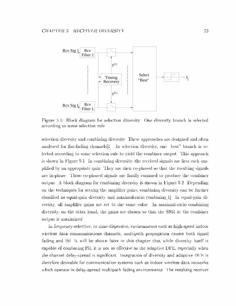
CHAPTER 5. RECEIVER DIVERSITY 73
Rcv Sig 1
τ(1)
τ(L)
xj
Rcv Sig L
Filter 1Rcv
Filter LRcv
TimingRecovery
Select"Best"
Figure 5.1: Block diagram for selection diversity. One diversity branch is selected
according to some selection rule.
selection diversity and combining diversity. These approaches are designed and often
analyzed for at-fading channels[1]. In selection diversity, one \best" branch is se-
lected according to some selection rule to yield the combiner output. This approach
is shown in Figure 5.1. In combining diversity, the received signals are �rst each am-
pli�ed by an appropriate gain. They are then co-phased so that the resulting signals
are in-phase. These co-phased signals are �nally summed to produce the combiner
output. A block diagram for combining diversity is shown in Figure 5.2. Depending
on the techniques for setting the ampli�er gains, combining diversity can be further
classi�ed as equal-gain diversity and maximal-ratio combining[1]. In equal-gain di-
versity, all ampli�er gains are set to the same value. In maximal-ratio combining
diversity, on the other hand, the gains are chosen so that the SNR at the combiner
output is maximized.
In frequency-selective, or time-dispersive, environments such as high-speed indoor
wireless data communications channels, multipath propagation causes both signal
fading and ISI. It will be shown later in this chapter that while diversity itself is
capable of combating ISI, it is not as e�ective as the adaptive DFE, especially when
the channel delay-spread is signi�cant. Integration of diversity and adaptive DFE is
therefore desirable for communication systems such as indoor wireless data networks
which operate in delay-spread multipath fading environments. The resulting receiver

CHAPTER 5. RECEIVER DIVERSITY 74
Rcv Sig 1
τ(1)
τ(L)
A 1
xj
Rcv Sig L
Filter 1Rcv
Filter LRcv
TimingRecovery
A L
Co-phase
Figure 5.2: Block diagram for combining diversity. The received signals are ampli�ed,
co-phased and summed.
structure is referred to as \adaptive diversity DFE," which can be further classi�ed
as \combining diversity DFE" and \selection diversity DFE." Combining diversity
DFE's are presented in this chapter, while selection diversity DFE's will be discussed
in Chapter 6.
5.1 Combining Diversity DFE
As previously mentioned, in a multipath fading environment where channel delay-
spread is signi�cant, it is desirable to extend conventional diversity techniques and
incorporate them into the adaptive DFE. A receiver structure for integrating combin-
ing diversity and adaptive DFE is shown in Figure 5.3. This structure, �rst proposed
by Monsen[59, 60], comprises one feedforward �lter in each diversity branch and a
common �lter for decision feedback. Since the ISI in di�erent diversity branches are
correlated, the �lters must be jointly optimized to take the ISI correlation into ac-
count. Both the channel-estimation-based adaptation (CEBA) and direct adaptation
(DA) algorithms, presented in Chapter 3, can be extended to accommodate receiver
diversity. For the CEBA approach, the mean-square error (MSE) between transmit-
ted symbol and output of the DFE (input of the slicer) is minimized. For the DA
approach, the weighted-square error (WSE) between transmitted symbol and output

CHAPTER 5. RECEIVER DIVERSITY 75
Rcv Sig 1y
j
AlignmentTiming
τ(1)
yj
τ(L)
∆y
j+
∆y
j+
FFF L FBF
xjz(k,k-1)
(1)∆ -sampleAdvance
∆(1)
∆(L)
(L)∆ -sampleAdvance
FFF 1Adapt.
Tap-Wt.(1)
(L)
Rcv Sig L
Filter 1Rcv
(1)
Filter LRcv
(L)
Figure 5.3: The maximal-ratio combining DFE.
of the DFE is minimized. Since both approaches attempt to minimize some measure
of the amount of unwanted component at the DFE output, this structure can be re-
garded as the equalized counterpart of maximal-ratio diversity combining. It will thus
be referred to as maximal-ratio combining decision-feedback equalizer (MRCDFE). If
the lengths of the feedforward �lters are set to 1 and that of the feedback �lter is set
to 0, then the MRCDFE degenerates into the conventional maximal-ratio diversity
combiner.
5.1.1 CEBA MRCDFE and Regularization
It is fairly straightforward to extend the CEBA algorithm of Chapter 3 to accommo-
date receiver diversity. Mathematically, the samples of the �ltered received signal of
the l-th diversity branch can be expressed as
y(l)j;k
= y(l)(jT + � (l) � kT
K) (5.1)
=Xi
xip(l)
(j � i)T + � (l) � kT
K
!+ n(l) q
jT + � (l) � kT
K
!; (5.2)
where j = 0; 1; : : :, k = 0; 1; : : : ; (K�1), and l = 1; 2; : : : ; L, with L being the number
of diversity branches. K is the number of samples taken per symbol period, and is

CHAPTER 5. RECEIVER DIVERSITY 76
assumed to be an integer. p(l)(�) in Equation 5.2 is the response, after being �ltered
by the receiver �lter, of the l-th branch channel to the transmitted pulse. n(l)(�) isthe AWGN in the l-th channel. � (l) in Equations 5.1 and 5.2 is the sampling instant
of the l-th diversity branch. Let
y(l)j
=
26666664
y(l)j;0
y(l)j;1
: : :
y(l)j;K�1
37777775
(5.3)
=Xi
xip(l)j�i + n
(l)j
(5.4)
where
p(l)i =
26666664
p(l)i;0
p(l)i;1
: : :
p(l)i;K�1
37777775; (5.5)
n(l)j=
26666664
n(l)j;0
n(l)j;1
: : :
n(l)j;K�1
37777775; (5.6)
p(l)i;k
= p(l) iT + � (l) � kT
K
!; (5.7)
and
n(l)i;k
= n(l) q
iT + � (l) � kT
K
!: (5.8)
Here \" denotes linear convolution de�ned in Equation 3.6. Then the output (equal-ized signal) z(j; k) of the adaptive DFE at time j using the �lter coe�cients obtained
at time k can be expressed as
z(j; k) =LXl=1
Nf�1Xi=0
w(l)�i;ky(l)
j+�(l)�i +NbXi=1
b�i;kx̂j�i; (5.9)
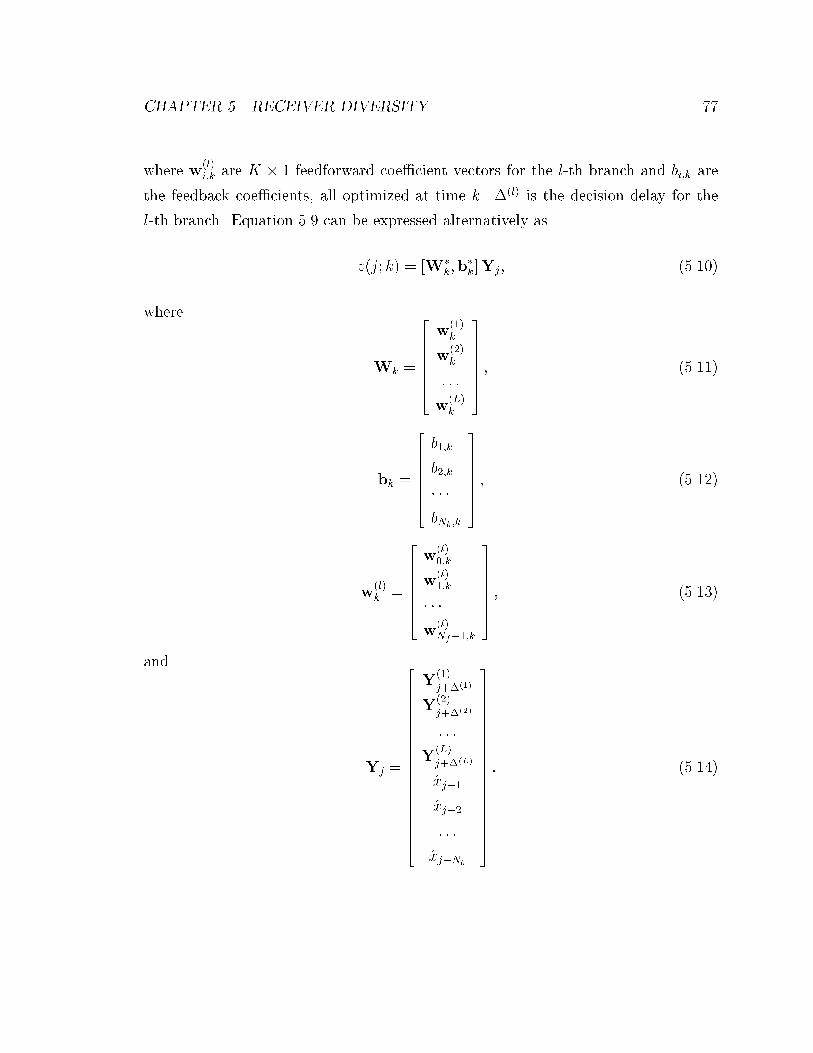
CHAPTER 5. RECEIVER DIVERSITY 77
where w(l)i;k
are K � 1 feedforward coe�cient vectors for the l-th branch and bi;k are
the feedback coe�cients, all optimized at time k. �(l) is the decision delay for the
l-th branch. Equation 5.9 can be expressed alternatively as
z(j; k) = [W�k;b�
k]Yj; (5.10)
where
Wk =
26666664
w(1)k
w(2)k
: : :
w(L)k
37777775; (5.11)
bk =
26666664
b1;k
b2;k
� � �bNb;k
37777775; (5.12)
w(l)k=
26666664
w(l)0;k
w(l)1;k
� � �w
(l)Nf�1;k
37777775; (5.13)
and
Yj =
266666666666666666664
Y(1)
j+�(1)
Y(2)
j+�(2)
: : :
Y(L)
j+�(L)
x̂j�1
x̂j�2
: : :
x̂j�Nb
377777777777777777775
: (5.14)

CHAPTER 5. RECEIVER DIVERSITY 78
In Equation 5.14, Y(l)
j+�(l) is given by
Y(l)
j+�(l) =
266666664
y(l)
j+�(l)
y(l)
j+�(l)�1
� � �y(l)
j+�(l)�Nf+1
377777775: (5.15)
For the CEBA approach, the channel pulse responses (CPR) for each diversity branch
are �rst estimated as described in Chapter 3. At every symbol period, after the CPR
estimates are obtained, the DFE �lter coe�cients are computed to minimize the
approximate MSE at the DFE output (input of the slicer), de�ned as
MSE(Wk;bk) = Ejxj � [W�k;b�
k]Yjj2: (5.16)
Note that Equation 5.16 is identical in form to Equation 3.32, therefore the corre-
sponding solution is similar to the solution for the single-branch case presented in
Chapter 3. Following the same derivations given in Chapter 3, it is straightforward
to show that the optimal DFE coe�cients are given by
Wk = (PP� �HH� +RN)�1� (5.17)
bk = �H�Wk (5.18)
where
P =
26666664
P(1)
P(2)
� � �P(L)
37777775; (5.19)
H = P
26664
0�1+1;Nb
INb
0�2+Nf�Nb�1;Nb
37775 ; (5.20)
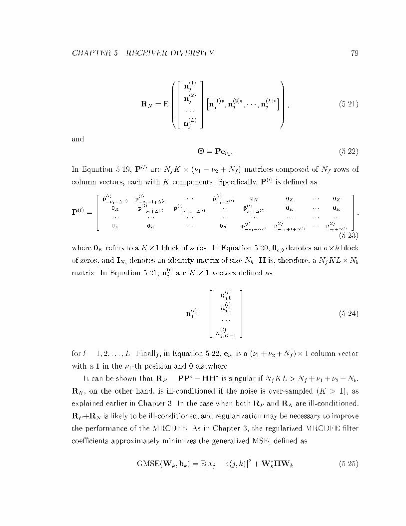
CHAPTER 5. RECEIVER DIVERSITY 79
RN = E
0BBBBBB@
26666664
n(1)j
n(2)j
� � �n(L)j
37777775hn(1)�j
;n(2)�j
; � � � ;n(L)�j
i1CCCCCCA; (5.21)
and
� = Pe�1: (5.22)
In Equation 5.19, P(l) are NfK � (�1 + �2 + Nf) matrices composed of Nf rows of
column vectors, each with K components. Speci�cally, P(l) is de�ned as
P(l) =
26664
p̂(l)
��1+�(l)
p̂(l)
��1+1+�(l)
� � � p̂(l)
�2+�(l)
0K 0K � � � 0K
0K p̂(l)
��1+�(l)
p̂(l)
��1+1+�(l)
� � � p̂(l)
�2+�(l)
0K � � � 0K
� � � � � � � � � � � � � � � � � � � � � � � �
0K 0K � � � 0K p̂(l)
��1+�(l)
p̂(l)
��1+1+�(l)
� � � p̂(l)
�2+�(l)
37775 ;
(5.23)
where 0K refers to a K�1 block of zeros. In Equation 5.20, 0a;b denotes an a�b block
of zeros, and INbdenotes an identity matrix of size Nb. H is, therefore, a NfKL�Nb
matrix. In Equation 5.21, n(l)j
are K � 1 vectors de�ned as
n(l)j=
26666664
n(l)j;0
n(l)j;1
� � �n(l)j;K�1
37777775
(5.24)
for l = 1; 2; : : : ; L. Finally, in Equation 5.22, e�1 is a (�1+�2+Nf )�1 column vector
with a 1 in the �1-th position and 0 elsewhere.
It can be shown that RP = PP��HH� is singular if NfKL > Nf + �1+ �2�Nb:
RN , on the other hand, is ill-conditioned if the noise is over-sampled (K > 1), as
explained earlier in Chapter 3. In the case when both RP and RN are ill-conditioned,
RP+RN is likely to be ill-conditioned, and regularization may be necessary to improve
the performance of the MRCDFE. As in Chapter 3, the regularized MRCDFE �lter
coe�cients approximately minimizes the generalized MSE, de�ned as
GMSE(Wk;bk) = Ejxj � z(j; k)j2 +W�k�Wk (5.25)

CHAPTER 5. RECEIVER DIVERSITY 80
where � is a positive-de�nite weighting matrix. The solution of this minimization
problem is given by
Wk = (PP� �HH� +RN +�)�1� (5.26)
bk = �H�Wk (5.27)
5.1.2 DA MRCDFE with Synthetic Training
For the DA approach, the LK � 1 vector
~Yj =
26666664
y(1)
j+�(1)
y(2)
j+�(2)
: : :
y(L)
j+�(L)
37777775
(5.28)
and the past decisions (transmitted symbols if available) are used to compute Wk
and bk using the least-squares lattice (LSL) algorithm given in Appendix C. Note
that the feedforward and feedback stages have dimensionalities KL and KL + 1,
respectively. If synthetic training is used, a synthetic training sequence (STS) can
�rst be produced for and prepended to the received signal samples from each branch
channel, as described in Chapter 3.
5.2 Simulation Results
The performance of the DA and CEBA MRCDFE are evaluated using bit-by-bit
computer simulation for both symbol-spaced (K = 1) and half-symbol-spaced (K =
2) cases. In each experiment, L sets of channel parameters are �rst independently
generated according to the previously mentioned distributions, where L is the number
of branch channels. A burst of 165 4-QAM symbols is generated and transmitted over
the wireless diversity channels according to Equation 2.17. The diversity channels are
assumed to be independent and have Gaussian power-delay pro�les with rms delay-
spreads of 50 ns and average delays of 200 ns. A square-root raised-cosine �lter with
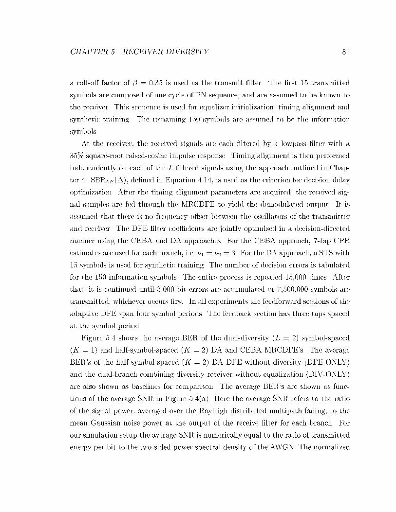
CHAPTER 5. RECEIVER DIVERSITY 81
a roll-o� factor of � = 0:35 is used as the transmit �lter. The �rst 15 transmitted
symbols are composed of one cycle of PN sequence, and are assumed to be known to
the receiver. This sequence is used for equalizer initialization, timing alignment and
synthetic training. The remaining 150 symbols are assumed to be the information
symbols.
At the receiver, the received signals are each �ltered by a lowpass �lter with a
35% square-root raised-cosine impulse response. Timing alignment is then performed
independently on each of the L �ltered signals using the approach outlined in Chap-
ter 4. SERLE(�), de�ned in Equation 4.14, is used as the criterion for decision delay
optimization. After the timing alignment parameters are acquired, the received sig-
nal samples are fed through the MRCDFE to yield the demodulated output. It is
assumed that there is no frequency o�set between the oscillators of the transmitter
and receiver. The DFE �lter coe�cients are jointly optimized in a decision-directed
manner using the CEBA and DA approaches. For the CEBA approach, 7-tap CPR
estimates are used for each branch, i.e. �1 = �2 = 3. For the DA approach, a STS with
15 symbols is used for synthetic training. The number of decision errors is tabulated
for the 150 information symbols. The entire process is repeated 15,000 times. After
that, it is continued until 3,000 bit errors are accumulated or 7,500,000 symbols are
transmitted, whichever occurs �rst. In all experiments the feedforward sections of the
adaptive DFE span four symbol periods. The feedback section has three taps spaced
at the symbol period.
Figure 5.4 shows the average BER of the dual-diversity (L = 2) symbol-spaced
(K = 1) and half-symbol-spaced (K = 2) DA and CEBA MRCDFE's. The average
BER's of the half-symbol-spaced (K = 2) DA DFE without diversity (DFE-ONLY)
and the dual-branch combining diversity receiver without equalization (DIV-ONLY)
are also shown as baselines for comparison. The average BER's are shown as func-
tions of the average SNR in Figure 5.4(a). Here the average SNR refers to the ratio
of the signal power, averaged over the Rayleigh distributed multipath fading, to the
mean Gaussian noise power at the output of the receive �lter for each branch. For
our simulation setup the average SNR is numerically equal to the ratio of transmitted
energy per bit to the two-sided power spectral density of the AWGN. The normalized

CHAPTER 5. RECEIVER DIVERSITY 82
10-1
10-2
10-3
10-4
-510
-610
Ave
rage
BE
R
15 2010Average SNR (dB)
DA (L=2,K=2)
DA (L=2,K=1)
CEBA (L=2,K=1)
DIV-ONLY
DFE-ONLY(DA,K=2)CEBA (L=2,K=2)
(a)
-510
10-4
10-3
10-2
10-1
Ave
rage
BE
R
0.25 0.5 0.75 1.0Normalized Delay-Spread
DA (L=2,K=2)
CEBA (L=2,K=1) DA (L=2,K=1)
DIV-ONLY(DA,K=2)
DFE-ONLYCEBA (L=2,K=2)
(b)
Figure 5.4: Average BER's of the unequalized diversity combiner (DIV-ONLY), half-
symbol-spaced DA DFE without diversity (DFE-ONLY), and dual diversity (L = 2)
DA and CEBA MRCDFE's: (a) as functions of average SNR at d = 0:5; and (b) as
functions of d at 15dB average SNR. The channel has a Gaussian power-delay pro�le
with a rms delay-spread of 50 ns and average delay of 200 ns.

CHAPTER 5. RECEIVER DIVERSITY 83
delay-spread d, de�ned in Equation 3.56, is at 0.5. For the DIV-ONLY case, the sig-
nals received from the diversity branches are co-phased and combined with weights
proportional to the received power averaged over the 165-symbol burst. Comparing
the DIV-ONLY case to the DFE-ONLY case, one can see that at d = 0:5, diver-
sity outperforms adaptive DFE when the average SNR is lower than 15 dB. This
is because when the average SNR is low, the performance is primarily AWGN- and
fading-limited. As mentioned previously, receiver diversity is very e�ective in a noise-
limited environment. Adaptive DFE, on the other hand, does not perform well against
AWGN. Furthermore, when the average SNR is low, decision errors occur often and
the error propagation associated with decision-feedback and decision-directed adap-
tation causes the DFE �lter coe�cients to diverge from the optimal values. When
the average SNR is higher than 15 dB, adaptive DFE outperforms the unequalized
diversity receiver. This is because in the high average SNR region, performance is
limited by the ISI. While receiver diversity is very e�ective against signal fading, it
is not as e�ective as the adaptive DFE in combating ISI.
Among the various MRCDFE's, it can be seen that both the symbol-spaced (K =
1) DA and CEBA MRCDFE with two branches (L = 2) outperform the DFE-ONLY
case by approximately 6�7 dB. Their performance gain over the DIV-ONLY case is
in excess of 10 dB. For the half-symbol-spaced (K = 2) case, on the other hand,
dual-diversity (L = 2) provides a gain of 7�8 dB over the DFE-ONLY case when the
DA approach is used to update the DFE �lter coe�cients. The performance gain over
the DIV-ONLY case is again more than 10 dB. However, when the CEBA approach
is used, the performance gain of the dual-diversity MRCDFE over the DFE-ONLY
case is only 2�3 dB. In fact, dual-diversity CEBA MRCDFE is slightly inferior to
the DIV-ONLY receiver when the average SNR is low.
The average BER's of the approaches shown in Figure 5.4(a) are plotted in Fig-
ure 5.4(b) as functions of the normalized delay-spread, with the average SNR �xed
at 15 dB. We can see that for d < 0:5, diversity combining outperforms DFE. This
is because for small values of d, the ISI introduced by multipath propagation is in-
signi�cant, and transmission errors are mainly caused by signal fading. Since receiver
diversity is more e�ective in combating fading, DIV-ONLY outperforms DFE-ONLY

CHAPTER 5. RECEIVER DIVERSITY 84
for low values of d. For values of d beyond 0.5, DFE-ONLY outperforms DIV-ONLY.
This is because as d increases, the multiple signals become more separated in delay,
thus causing a signi�cant amount of ISI. An adaptive DFE with su�cient number
of �lter taps is capable of resolving and combining constructively the multiple signal
copies, thus bene�ting from the time diversity implicit in multipath propagation. An
unequalized diversity combiner, on the other hand, is not as e�cient in coping with
ISI. Therefore the DFE-ONLY outperforms DIV-ONLY when d is large.
Among the MRCDFE's, the dual-diversity (L = 2) symbol-spaced (K = 1) DA
and CEBA MRCDFE's achieve average BER's that are almost two orders of mag-
nitude lower than that of the DFE-ONLY case. Compared to the DIV-ONLY case,
dual-diversity symbol-spaced DA and CEBA MRCDFE's achieve average BER's that
are between one to two orders of magnitude lower. The dual-diversity (L = 2)
half-symbol-spaced (K = 2) DA MRCDFE also attains a much better performance
than the DIV-ONLY and DFE-ONLY cases. However, the BER of the dual-diversity
(L = 2) half-symbol-spaced (K = 2) CEBA MRCDFE is less than one order of
magnitude lower than that of DFE-ONLY only when d < 0:8. For d > 0:8, the dual-
diversity half-symbol-spaced CEBA MRCDFE performs worse than the DFE-ONLY
case. Furthermore, the dual-diversity half-symbol-spaced CEBA MRCDFE is inferior
to the DIV-ONLY receiver for values of d close to 0.25 and 1.0. The poor performance
of the fractionally-spaced CEBA MRCDFE is due to the poor numerical properties of
the MMSE solution, as explained in Chapter 3. As will be shown later, this problem
can be remedied using regularization.
It can also be seen from Figure 5.4 that for the dual-diversity (L = 2) cases, the
general conclusions obtained in Chapter 3 regarding the relative performance of the
CEBA and DA approaches also apply. In particular, we �nd that 1) DA slightly out-
performs CEBA for symbol-spaced MRCDFE's when the amount of channel delay-
spread is moderate; 2) DA signi�cantly outperforms CEBA for fractionally-spaced
cases regardless of delay-spread; and 3) CEBA is more sensitive to the variations
in delay-spread, therefore both symbol-spaced and fractionally-spaced CEBA MR-
CDFE's become signi�cantly inferior to the DA MRCDFE if the delay-spread is
increased. These observations can be explained using arguments similar to those

CHAPTER 5. RECEIVER DIVERSITY 85
presented in Chapter 3.
The average BER of the dual-diversity (L = 2) half-symbol-spaced (K = 2)
CEBA MRCDFE with regularization is shown in Figure 5.5. In Figure 5.5(a), the
BER's are shown as functions of the average SNR, with normalized delay-spread
d = 0:5. In Figure 5.5(b), the BER's are shown as functions of the normalized delay-
spread, with an average SNR of 15 dB. The BER's of the dual-diversity symbol-
spaced (K = 1) CEBA MRCDFE and half-symbol-spaced DA and CEBA MRCDFE
without regularization are also repeated here. The BER of the DFE-ONLY case is
also shown. It can again be seen that regularization is very e�ective in improving the
performance for half-symbol-spaced CEBA MRCDFE's. For example, with d = 0:5,
at high average SNR regularization improves the performance of the K = 2 CEBA
MRCDFE by 6 dB1. With regularization, the performance gain of the dual-diversity
(L = 2) CEBA MRCDFE over the DFE-ONLY case is 7�8 dB at d = 0:5. At 15 dB
average SNR, the average BER of the dual-diversity (L = 2) CEBA MRCDFE with
regularization is approximately two orders of magnitude lower than the DFE-ONLY
case for 0:25 < d < 0:75. However, regularized CEBA MRCDFE remains sensitive to
variations in d. As mentioned previously, this is because �xed-length CPR estimates
are used to synthesize the regularized DFE coe�cients. When d is large the estimate
is biased, resulting in DFE �lter coe�cients that are signi�cantly inferior to the DA
solution.
5.3 Summary
High-speed indoor wireless data networks encounter both signal fading and channel
delay-spread. Adaptive DFE has been shown in Chapter 3 to be very e�ective against
the performance degradation due to the ISI caused by channel delay-spread. How-
ever, when the average SNR is low, the performance of an adaptive DFE is limited
by signal fading. Receiver diversity, on the other hand, is a technique commonly
used in wireless communication systems to combat signal fading. Diversity uses more
1A gain of 2dB was obtained for the DFE-ONLY case in Chapter 3.

CHAPTER 5. RECEIVER DIVERSITY 86
10-1
10-2
10-3
10-4
-510
-610
Ave
rage
BE
R
15 2010Average SNR (dB)
DA (L=2,K=2)
(L=2, K=2)CEBA/REG
CEBA (L=2,K=2)
CEBA (L=2,K=1)
DFE-ONLY(DA,K=2)
(a)
-510
10-4
10-3
10-2
10-1
Ave
rage
BE
R
0.25 0.5 0.75 1.0Normalized Delay-Spread
DA (L=2,K=2)
CEBA/REG(L=2,K=2)CEBA (L=2,K=1)
CEBA (L=2,K=2)
DFE-ONLY(DA,K=2)
(b)
Figure 5.5: Average BER's of the half-symbol-spaced DA DFE without diversity
(DFE-ONLY), dual diversity (L = 2) DA MRCDFE, and dual diversity (L = 2)
CEBA MRCDFE with regularization: (a) as functions of average SNR at d = 0:5;
and (b) as functions of d at 15dB average SNR. The channel has a Gaussian power-
delay pro�le with a rms delay-spread of 50 ns and average delay of 200 ns.
CHAPTER 5. RECEIVER DIVERSITY 87
than one radio transmission channel to convey the same message. The e�ect of sig-
nal fading can be mitigated if the signals from the diversity branches are properly
combined. Although diversity is very e�ective against signal fading, it alone cannot
yield satisfactory performance in a time-dispersive, or frequency-selective, fading en-
vironment. Integration of diversity and adaptive equalization is therefore desirable
for communication systems such as indoor wireless data networks which operate in a
delay-spread multipath fading environment.
Receiver diversity can be classi�ed according to the techniques used to combine
the branch signals. The simplest form of diversity combining is selection diversity.
In selection diversity, one branch is selected as the combiner output according to
some selection rule. Another diversity approach is combining diversity, in which the
weighted sum of the co-phased branch signals is used as the combiner output. These
techniques were designed and often analyzed for at-fading environments, and must
be modi�ed to accommodate equalization in order to yield satisfactory performance
in a time-dispersive fading environment. The integration of combining diversity and
adaptive DFE can be achieved using a structure referred to in this dissertation as
the maximal-ratio combining DFE (MRCDFE). This structure comprises multiple
feedforward �lters and a common feedback �lter, which are jointly optimized using
the CEBA or DA algorithms. The extension of these algorithms are described in this
chapter.
Simulation results show that the MRCDFE can achieve a signi�cant performance
gain over both the adaptive DFE without diversity and the unequalized diversity re-
ceiver. In particular, for 50% normalized delay-spread, a gain of 6�8 dB is achieved
over the adaptive DFE without diversity. The gain over the unequalized diversity
receiver is in excess of 10 dB. The relative performance of the CEBA and DA MR-
CDFE's are also analyzed, and it is found that the general conclusions obtained in
Chapter 3 also apply. Furthermore, just as in Chapter 3, half-symbol-spaced CEBA
MRCDFE encounters numerical di�culties in computing the minimum mean-square
error (MMSE) �lter coe�cients. Regularization is shown to be an e�ective remedy
for this situation, and is very e�ective in improving the performance of fractionally-
spaced CEBA MRCDFE's.

Chapter 6
MAP Selection Diversity DFE
The maximal ratio combining DFE (MRCDFE) presented in Chapter 5 integrates
adaptive DFE and combining diversity. While it is very e�ective in mitigating the
e�ects of multipath propagation, the MRCDFE is computationally intensive because
the branch DFE �lter coe�cients are jointly optimized. Integration of adaptive DFE
and selection diversity, on the other hand, provides a simpler alternative because
the branch DFE's can be individually optimized if selection diversity is used. A
wide variety of approaches exist for integrating selection diversity and equalization.
For example, selection diversity could be performed at the input or output of the
equalizer[61], as shown in Figure 6.1. Furthermore, selection could be performed on
a per-frame or per-symbol basis[61], as shown in Figure 6.2. The metric for selec-
tion is also an extremely important design parameter, and di�erent choices have been
investigated[62, 63, 64]. In general the \best" choice will depend, among other fac-
tors, on the characteristics of the channel, adaptive equalization algorithm, equalizer
structure, and tolerable computational complexity. For adaptive DFE's operating on
indoor high-speed wireless radio links, symbol-by-symbol selection at the DFE output
(input of the decision device) is attractive. This approach, shown in Figure 6.3, will
be referred to as the selection diversity DFE (SDDFE). First, indoor high-speed wire-
less radio links generally have low mobile speed and short symbol period. Thus the
channels are approximately time-invariant. This simpli�es the design of the selection
metric. Secondly, the �lter coe�cients of an adaptive DFE are updated at the end
88
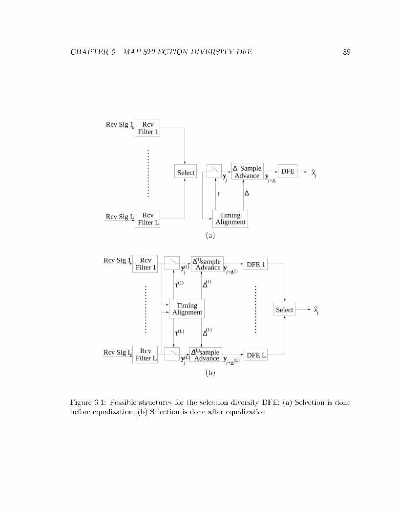
CHAPTER 6. MAP SELECTION DIVERSITY DFE 89
Rcv Sig 1
∆y
j+
DFE xjAdvanceSample∆
Rcv Sig L
Filter 1Rcv
Filter LRcv
Select
AlignmentTiming
yj
τ ∆
(a)
DFE L
DFE 1Rcv Sig 1
yj ∆
yj+
AlignmentTiming
τ(1) ∆(1)
yj ∆
yj+
τ(L) ∆(L)
Select xj
(1)∆ -sampleAdvance
(L)∆ -sampleAdvance
Rcv Sig L
Filter 1Rcv
(1)(1)
Filter LRcv
(L)(L)
(b)
Figure 6.1: Possible structures for the selection diversity DFE: (a) Selection is done
before equalization; (b) Selection is done after equalization.

CHAPTER 6. MAP SELECTION DIVERSITY DFE 90
Per-frame selection Symbol-by-symbol selection
Figure 6.2: Possible selection schemes for the SDDFE.
Rcv Sig 1y
j
AlignmentTiming
τ(1) ∆(1)
yj
τ(L) ∆(L)
(1)∆ -sampleAdvance
(L)∆ -sampleAdvance
zk(1)
zk(L)
FinalDecision
θk(L)
θk(1)
FFF 1
FFF L
Feedback L
Feedback 1
SelectionMetric 1
SelectionMetric L
Tap-Wt.Adapt. L
Tap-Wt.Adapt. 1
Per-symSelect
∆y
j+
∆y
j+
Rcv Sig L
Filter 1Rcv
(1)
Filter LRcv
(L)
(1)
(L)
Figure 6.3: Selection-diversity decision-feedback equalizer.

CHAPTER 6. MAP SELECTION DIVERSITY DFE 91
of every symbol period. In this case symbol-by-symbol selection diversity can, with
a properly designed selection rule, dynamically select the equalizer which will yield a
lower probability of error. Selection on a per-frame basis, in contrast, locks on to one
particular branch DFE even when it is outperformed by other branch DFE's some
time after the selection is done. Thirdly, symbol-by-symbol selection makes possi-
ble the feedback and adaptation structure shown in Figure 6.3. More speci�cally, at
the end of every symbol period the �nal (and hence more reliable) decision is fed
back through the feedback sections to all branch DFE's. It is also used to adapt
the DFE �lter settings for all diversity branches. This should somewhat mitigate the
e�ect of error propagation in decision-directed adaptive DFE's. It was also shown
that while the MRCDFE is theoretically very e�cient in suppressing both ISI and
signal-fading, when some timing alignment parameters are not chosen properly, the
MRCDFE may in fact have a poorer performance than certain selection diversity
combining approaches if the number of training symbols is limited[43, 63]. Finally,
SDDFE has the merit of having lower complexity than MRCDFE, especially when a
simple selection metric is used[62].
In this chapter, we investigate the SDDFE for the direct adaptation (DA) least-
squares lattice (LSL) DFE. While this structure has been proposed and analyzed
by previous researchers[61, 62], in this chapter selection is performed at the bit-
level instead of the symbol-level. We also develope a new selection metric based
on a maximum a posteriori probability (MAP) selection rule, which is shown to be
optimal for a SDDFE in the MAP sense. Simulation results show that the new
method developed in this chapter is very e�ective. In particular, a gain of as high as
2 dB in average signal-to-noise ratio (SNR) over a conventional scheme is achieved.
The new scheme is also compared to the MRCDFE, and the results show that the
new approach can achieve almost the same performance as the MRCDFE with lower
computational complexity.
CHAPTER 6. MAP SELECTION DIVERSITY DFE 92
6.1 Selection Diversity DFE
The selection diversity DFE (SDDFE) is shown in Figure 6.3. It consists of L branch
DFE's, a selection metric estimator, a selection combiner, and a decision device. At
the end of every symbol period the output of one branch DFE is selected according
to the estimated selection metric. Note that selection is done at the bit-level, i.e.
the in-phase (real part) and the quadrature-phase (imaginary part) components of
the SDDFE output are independently selected and may come from di�erent branch
DFE's. The selected output is passed on to the decision device to obtain the de-
modulated symbol. This �nal and hence more reliable decision is then used as the
input to the feedback sections of the DFE's and to adapt the DFE �lter settings in a
decision-directed manner. The branch DFE's are individually adapted using the DA
algorithm of Chapter 3.
SDDFE has been proposed and analyzed in several previous researches[61, 62, 63].
However, our approach presented here di�ers from the previously proposed approaches
in two signi�cant aspects. First, in our approach selection is done at the bit-level in-
stead of symbol-level as previously proposed. Intuitively this should result in a better
performance provided that an e�ective metric for selection is used. Secondly, the
selection metric used in this dissertation is derived from the maximum a posteriori
(MAP) selection rule. Conceptually, the a posteriori probabilities of correctly de-
tecting the in-phase (quadrature-phase) information symbol component conditioned
solely on the real part (imaginary part) of one branch DFE output are �rst estimated
for all L diversity branches. The real part (imaginary part) of the branch DFE output
with the highest a posteriori probability of begin correct is then used to produce the
in-phase (quadrature-phase) component of the �nal decision. This is considerably dif-
ferent from the previously described approaches[61, 62, 63], where selection is based
on the average di�erence between the input and output of the decision device. In
fact, as proved in Appendix D, the MAP selection rule is optimal for a SDDFE in
the MAP sense, i.e. it maximizes the conditional probability of making a correct �nal
decision given all the outputs of the branch DFE's. Furthermore, as will be shown in
Section 6.2, the selection metric resulting from the MAP selection rule is very simple

CHAPTER 6. MAP SELECTION DIVERSITY DFE 93
under a certain assumption on the distribution of the ISI.
6.2 MAP Selection Metric for SDDFE
The mathematical derivation for the MAP selection metric will be presented in this
section. The derivations presented here are equally applicable for the real (in-phase)
and imaginary (quadrature-phase) components. For signal constellations such as
square QAM, the same formula for selection metric can be applied for the in-phase
and quadrature-phase components. In the general case di�erent formulae will have
to be used for di�erent components. The extension to these cases are, however,
straightforward. In order to simplify notations, in this chapter we use bold-face
symbols to denote complex quantities, while plain-text symbols are used to denote
generically the real or imaginary part of the complex quantity being considered. For
example, the transmitted information symbol xk is a complex quantity which takes
values of f1 + j; 1 � j;�1 + j;�1 � jg. xk is therefore the real or imaginary part ofxk and takes values of f�1;+1g. It should be kept in mind that all quantities in this
chapter are scalar quantities.
Consider L independent diversity branches equalized by the SDDFE as shown
in Figure 6.3. The a posteriori probability of correct detection for the l-th DFE
conditioned solely on its output can be expressed as
P(l)k(z
(l)k) = Prob
hx̂(l)k= xkjz(l)k was observed
i; (6.1)
where xk is the transmitted symbol at time k, x̂(l)k
is the decision of the l-th branch
DFE based on its output z(l)k
according to some decision rule. Using Bayes' rule
Equation 6.1 can be rewritten as
P(l)k(z
(l)k) =
24f (l)k
(z(l)kjxk = x̂
(l)k)
f(l)k(z
(l)k)
35� Prob[xk = x̂
(l)k]
= �(l)k� Prob[xk = x̂
(l)k]; (6.2)

CHAPTER 6. MAP SELECTION DIVERSITY DFE 94
where f(l)k(�j�) and f
(l)k(�) are the conditional and marginal probability density func-
tions (pdf) of z(l)k, respectively, and �
(l)k
is the ratio of the two. The MAP selection
rule selects as the �nal decision the output of the branch with the highest a posteriori
probability of being correct. Throughout this dissertation we will assume xk to be
uniformly distributed, therefore Prob[xk = x̂(l)k] is the same for all l. Hence the MAP
selection rule can equivalently be expressed as
x̂k = x̂(l)k
if �(l)k� �
(m)k
for all m 6= l. (6.3)
Assuming that the fedback decisions are error-free, the equalizer output z(l)k
of the
l-th diversity branch can be expressed as
z(l)k
= �(l)kxk + �
(l)k
(6.4)
where
�(l)k= Re
8<:Ehz(l)kx�k
iEhjxkj2
i9=; (6.5)
and �(l)k
is the noise component which is uncorrelated with xk, i.e.
E[xk�(l)k] = 0 (6.6)
For a multipath channel with AWGN, �(l)k
consists of the residual ISI, cross-talk
between the in-phase or quadrature-phase component, and �ltered Gaussian noise.
In general the exact distribution of �(l)k
is, if at all possible, very di�cult to obtain.
However, we will assume �(l)kto be zero-mean Gaussian random variables with variance
�(l)2k
. One reason for making this assumption is that for a static channel and time-
invariant DFE, �(l)k
is a sum of several zero-mean uncorrelated random variables, and
its distribution will be approximately Gaussian if the number of summands is large.
The multipath fading channel that is being considered here is, though not static,
very slowly varying. The Gaussian assumption greatly simpli�es the mathematics.
Then, as will be shown later, the resulting metric for selection proves to be e�ective
in signi�cantly reducing the average BER, further justifying the assumption.

CHAPTER 6. MAP SELECTION DIVERSITY DFE 95
Under the assumption of Gaussian distributed �(l)k, it is straightforward to derive
a formula for �(l)k. In particular, we have
f(l)k
�z(l)kjxk = x̂
(l)k
�=
1p2��
(l)k
exp
0B@�
�z(l)k� �
(l)kx̂(l)k
�22�
(l)2k
1CA (6.7)
For the 4-QAM modulation that is being considered here, we have
x̂(l)k=
8<: 1 if z
(l)k� 0
�1 if z(l)k
< 0: (6.8)
Therefore,
f(l)k
�z(l)k
�=
1p2��
(l)k
26412exp
0B@�
�z(l)k� �
(l)k
�22�
(l)2k
1CA+
1
2exp
0B@�
�z(l)k+ �
(l)k
�22�
(l)2k
1CA375 ; (6.9)
thus
�(l)k=
2
1 + e�2�(l)
k
; (6.10)
where
�(l)k=
�(l)k
���z(l)k
����(l)2k
: (6.11)
Therefore the MAP selection rule for the new SDDFE is
x̂k = x̂(l)k
if �(l)k� �
(m)k
; for all m 6= l. (6.12)
where �(l)k
is the selection metric de�ned in Equation 6.11. Note that this metric
depends on the statistical parameters �(l)k
and �(l)2k
which, as will be discussed in
Sections 6.3, can be easily computed during the adaptation process.

CHAPTER 6. MAP SELECTION DIVERSITY DFE 96
6.3 Computation of Selection Metric
In order to make use of the MAP selection rule, the parameters �(l)k
and �(l)2k
must
be estimated. For simplicity we will omit the superscript \(l)" since it is understood
that these parameters are independently estimated for each diversity branch. We will
also use the notations �k and �2kto denote the statistical parameters and �̂k and �̂2
k
to represent the estimates of the statistical parameters.
To obtain an estimate for �2k, we start with the lowpass-�ltered squared one-step
output error (FSE), de�ned as
Ek = LPFk
hjzj � xjj2
i; (6.13)
where zj and xj are the output of the DFE and transmitted symbol, respectively,
and the operator LPFk [gj] denotes the output at time k of a lowpass �lter with
input signal gj. This quantity is simple to calculate and has previously been used
alone[62] as the selection metric for SDDFE. In this dissertation, a �rst-order single-
pole lowpass �lter with coe�cient 0.5 is used. This number is chosen empirically based
on some preliminary simulations on SDDFE using FSE alone as the selection metric1.
As will be shown by simulation, using FSE alone as the selection metric yields worse
average BER performance than the metrics developed in this dissertation.
Since Ek consists of the weighted sum of quantities which are correlated with the
signal xk, it cannot be used directly as an estimate of �2k, and �k must be estimated
�rst. A candidate for the decision-directed estimate of �k would be
�̂k = Re
8<:LPFk
hzjx
�j
iLPFk
hjxjj2
i9=; (6.14)
1Note that the same �lter coe�cient is used for the FSE-based MAP selection metric which will
be discussed later. While this coe�cient is not optimized for the MAP metric, it was observed that
varying the low-pass �lter coe�cient does not change signi�cantly the average BER of the FSE-based
MAP metric.
CHAPTER 6. MAP SELECTION DIVERSITY DFE 97
Then we would have
�̂2k=
1
2
nEk � (1� �̂k)
2LPFk
hjxjj2
io: (6.15)
However, since the FSE is not minimized at every time k by the LSL algorithm,
Equations 6.14 and 6.15 cannot be further simpli�ed and explicit evaluation of both
estimates is required.
In order to eliminate the need to estimate both �k and �2k, we make use of the
weighted-square error (WSE) Jk de�ned in Equation 3.52. Speci�cally, let
�̂k = Re
24Pk
j=0 �k�jz(j; k)x�
jPk
j=0 �k�j jxjj2
35 (6.16)
and
�̂2k=
1
2
24Jk � (1� �̂k)
2kX
j=0
�k�j jxjj235 ; (6.17)
where z(j; k) was de�ned in Section 3.1. As previously mentioned Jk is minimized
at every k by the LSL algorithm, therefore it can be shown by the orthogonality
principle[38] that
�̂k =
Pk
j=0 �k�j jxjj2 � JkP
k
j=0 �k�j jxjj2
(6.18)
and
�̂2k=
�̂kJk
2; (6.19)
thus
�k =2 jzkjJk
: (6.20)
It can be seen from Equation 6.20 that this metric for diversity selection depends only
on Jk and jzkj, therefore the need to evaluate Equations 6.18 and 6.19 is eliminated.
Three important points are worth noting. First, the evaluation of Equations 6.13,
6.14 and 6.15 requires the knowledge of the transmitted symbol xk at the receiver. Of
course this information is unavailable except during training. Therefore, whenever xk
is unknown, these equations are evaluated with xk replaced by x̂k. Secondly, while the

CHAPTER 6. MAP SELECTION DIVERSITY DFE 98
WSE Jk could be evaluated explicitly from Equation 3.52, in the LSL algorithm Jk
is computed recursively in a decision-directed manner, and can in fact be considered
as a by-product of adaptation. Thirdly, a multiplicative factor that only depends
on � and k should be introduced in Equation 6.19 in order to make the estimate
approximately unbiased. However, since this factor is common to all branches, we
have simply set it to 1 for all k, i.e. we have normalized it out of all branches since
comparisons are among branches only.
6.4 Simulation Results
The performance of the proposed new selection diversity scheme is evaluated using
bit-by-bit computer simulation. The number of diversity branches L is �xed at 2
although the approach applies to any number of diversity branches. In all experiments
the feedforward �lter of the adaptive DFE has 8 taps, spaced at half the symbol-
period. The feedback �lter has 3 taps spaced at the symbol period. Only the half-
symbol-spaced DA DFE is simulated because it was observed in Chapter 3 and 5 to
have the best BER performance over a wide range of channel conditions. In each
experiment, L sets of channel parameters are �rst independently generated according
to the previously mentioned distributions, and a burst of 165 4-QAM symbols is
generated and transmitted over the diversity channels according to Equation 2.17. A
square-root raised cosine �lter with a roll-o� factor of � = 0:35 is used as the transmit
�lter. The �rst 15 transmitted symbols are composed of one cycle of PN sequence,
and are assumed to be known to the receiver. This sequence is used for equalizer
initialization, timing alignment, and synthetic training. The remaining 150 symbols
are assumed to be the information symbols.
At the receiver, the received signals are each �ltered by a lowpass �lter with a
35% square-root raised-cosine impulse response. Timing alignment is then performed
independently on each of the L �ltered signals using the approach outlined in Chap-
ter 4. SERLE(�), de�ned in Equation 4.14, is used as the metric for decision delay
optimization. After the timing alignment parameters are acquired, the received sig-
nal samples are fed through the SDDFE to yield the demodulated output. It is

CHAPTER 6. MAP SELECTION DIVERSITY DFE 99
assumed that there is no frequency o�set between the oscillators of the transmitter
and receiver. The DFE �lter coe�cients are optimized in a decision-directed manner
using the DA approach. A synthetic training sequence (STS) with 15 symbols is also
used for synthetic training. The number of decision errors is tabulated for the 150
information symbols. The entire process is repeated 15,000 times. After that, it is
continued until 3,000 bit errors are accumulated or 7,500,000 symbols are transmitted,
whichever occurs �rst.
The three selection metrics simulated are: 1) the FSE de�ned in Equation 6.13;
2) the FSE-based MAP metric (FSE/MAP) de�ned in Equations 6.14 and 6.15; and
3) the WSE-based MAP metric (WSE/MAP) de�ned in Equation 6.20. In addition,
an \ideal" selection scheme is also simulated in which a decision error occurs only
when all diversity branch decisions are wrong. This is not implementable since it
assumes knowledge of the symbol transmitted, but it represents the \best" possible
performance for any selection diversity scheme. The performance of the two-branch
MRCDFE as well as DFE-only (L = 1) and diversity-only (unequalized) cases are
also simulated in order to provide a baseline for comparison. For the unequalized
case two-branch selection diversity is performed using the received signal power as
selection metric.
Figure 6.4 shows the average BER for the various selection metrics as a func-
tion of the average SNR. As in Chapter 5, the average SNR is numerically equal to
the ratio of transmitted energy per bit to the two-sided power spectral density of
the AWGN. Here the channel is assumed to have an exponential power-delay pro-
�le with a rms delay-spread of 50 ns2. The normalized delay-spread d, de�ned in
Equation 3.56, is set at 0.5. It can be seen from this �gure that in the region sim-
ulated, the MAP metrics signi�cantly outperform the FSE metric. In particular, at
high SNR the FSE/MAP metric achieves a gain of approximately 0.75 dB in average
SNR over the FSE metric. Furthermore, WSE/MAP achieves an additional gain of
0.5�1 dB over FSE/MAP, and is 1�2 dB better than FSE. The di�erence between
the FSE/MAP and WSE/MAP metrics lies in the method by which �k and �2kare
2Recall that, for the channel model used, this implies that the path delays are generated from an
exponential distribution with a standard deviation of 50 ns.

CHAPTER 6. MAP SELECTION DIVERSITY DFE 100
12 14 16 18 2010Average SNR
10-6
10-5
10-4
10-3
10-2
10-1
100
Ave
rage
BE
R FSE/MAPWSE/MAP
MRCDFE
IDEAL
FSE
Figure 6.4: Average BER's of the various selection metrics as functions of the average
SNR. The channel has an exponential power-delay pro�le with a rms delay-spread of
50 ns. The normalized delay spread d is 0.5. As noted in the text, the IDEAL case
is not realizable.
estimated. FSE/MAP makes use of time-averaged (lowpass-�ltered) squared one-step
output error to obtain estimates of these parameters (see Equations 6.13, 6.14, and
6.15). However, since the adaptive DFE is a time-varying �lter, the squared one-step
output error in Equation 6.13 is a non-stationary random process. Therefore the FSE
obtained from Equation 6.13 is not an accurate estimate of the mean-square error
(MSE). On the other hand, WSE/MAP makes use of the WSE, Jk, de�ned in Equa-
tion 3.52. As shown in Equation 3.52, at every time k, Jk is the \time average" of
squared output error in estimating xj, j = 0; 1; : : : ; k, using the DFE settings of time
k. This is a better estimate of the true MSE since, conceptually, the DFE settings
are \frozen" when computing the time average in Equation 3.52, making the error
power process being averaged stationary. The additional gain of 0.5�1 dB achieved
by WSE/MAP over FSE/MAP justi�es this interpretation.
It can also be seen from Figure 6.4 that MRCDFE achieves a lower average BER
than SDDFE for all average SNR's simulated, regardless of selection metric. This is
di�erent from previously reported results[43], where it was found that MRCDFE is
inferior to SDDFE with FSE/MAP or WSE/MAP metrics when the average SNR is
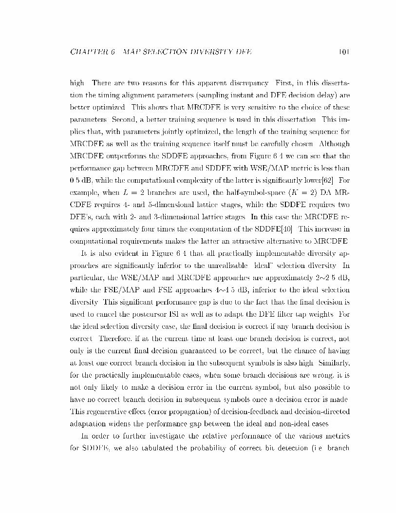
CHAPTER 6. MAP SELECTION DIVERSITY DFE 101
high. There are two reasons for this apparent discrepancy. First, in this disserta-
tion the timing alignment parameters (sampling instant and DFE decision delay) are
better optimized. This shows that MRCDFE is very sensitive to the choice of these
parameters. Second, a better training sequence is used in this dissertation. This im-
plies that, with parameters jointly optimized, the length of the training sequence for
MRCDFE as well as the training sequence itself must be carefully chosen. Although
MRCDFE outperforms the SDDFE approaches, from Figure 6.4 we can see that the
performance gap between MRCDFE and SDDFE with WSE/MAP metric is less than
0.5 dB, while the computational complexity of the latter is signi�cantly lower[62]. For
example, when L = 2 branches are used, the half-symbol-space (K = 2) DA MR-
CDFE requires 4- and 5-dimensional lattice stages, while the SDDFE requires two
DFE's, each with 2- and 3-dimensional lattice stages. In this case the MRCDFE re-
quires approximately four times the computation of the SDDFE[40]. This increase in
computational requirements makes the latter an attractive alternative to MRCDFE.
It is also evident in Figure 6.4 that all practically implementable diversity ap-
proaches are signi�cantly inferior to the unrealizable \ideal" selection diversity. In
particular, the WSE/MAP and MRCDFE approaches are approximately 2�2.5 dB,
while the FSE/MAP and FSE approaches 4�4.5 dB, inferior to the ideal selection
diversity. This signi�cant performance gap is due to the fact that the �nal decision is
used to cancel the postcursor ISI as well as to adapt the DFE �lter tap weights. For
the ideal selection diversity case, the �nal decision is correct if any branch decision is
correct. Therefore, if at the current time at least one branch decision is correct, not
only is the current �nal decision guaranteed to be correct, but the chance of having
at least one correct branch decision in the subsequent symbols is also high. Similarly,
for the practically implementable cases, when some branch decisions are wrong, it is
not only likely to make a decision error in the current symbol, but also possible to
have no correct branch decision in subsequent symbols once a decision error is made.
This regenerative e�ect (error propagation) of decision-feedback and decision-directed
adaptation widens the performance gap between the ideal and non-ideal cases.
In order to further investigate the relative performance of the various metrics
for SDDFE, we also tabulated the probability of correct bit detection (i.e. branch

CHAPTER 6. MAP SELECTION DIVERSITY DFE 102
12 14 16 18 2010Average SNR
96
98
100
94
82
90
92
88
86
84
FSE
FSE/MAP
WSE/MAPPr
ob. o
f C
orre
ct D
ecis
ion
(%)
Figure 6.5: Conditional probability of correct branch selection given that exactly
one diversity branch decision is wrong. The channel has an exponential power-delay
pro�le with a rms delay-spread of 50 ns. The normalized delay-spread d is 0.5.
selection) given that exactly one of the diversity branch decisions is wrong. This
conditional probability re ects the ability of the selection metric to correctly assess
the reliability of the diversity branch decisions. The results for the various selection
metrics are shown in Figure 6.5 as a function of the average SNR. Note that by de�-
nition this probability is always 100% for the ideal case, and that it is not applicable
to MRCDFE because the branch DFE's in MRCDFE are jointly optimized. It can be
seen that, in comparison to the FSE metric, MAP metrics provide better indications
of the reliability of the diversity branch decisions, with WSE/MAP being better than
FSE/MAP, as was inferred from the error performance earlier.
The average BER of the various diversity DFE's are also shown in Figure 6.6
as a function of the normalized delay-spread with the average SNR set to 15 dB.
The channel is still assumed to have an exponential power-delay pro�le. The aver-
age BER's for the DFE-only (L = 1) and diversity-only (unequalized) cases are also
shown for comparison. Several observations are noteworthy on this �gure. First, at
15dB SNR, with 0:25 � d � 0:6, two-branch unequalized selection diversity outper-
forms one-branch DFE. However, as d increases beyond 0.6, one-branch DFE is more
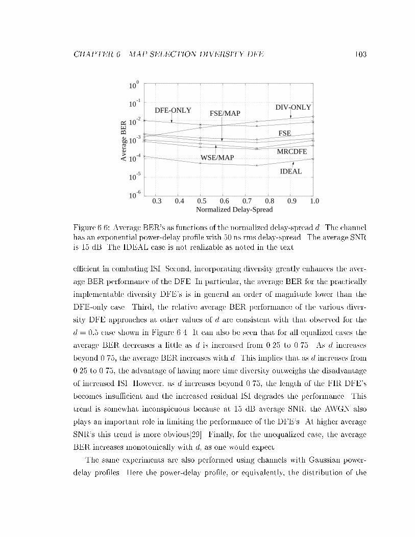
CHAPTER 6. MAP SELECTION DIVERSITY DFE 103
10-6
10-5
10-4
10-3
10-2
10-1
100
Ave
rage
BE
R
0.3 0.4 0.5 0.6 0.7 0.8 0.9 1.0Normalized Delay-Spread
MRCDFEWSE/MAP
DFE-ONLY DIV-ONLY
IDEAL
FSE/MAP
FSE
Figure 6.6: Average BER's as functions of the normalized delay-spread d. The channel
has an exponential power-delay pro�le with 50 ns rms delay-spread. The average SNR
is 15 dB. The IDEAL case is not realizable as noted in the text.
e�cient in combating ISI. Second, incorporating diversity greatly enhances the aver-
age BER performance of the DFE. In particular, the average BER for the practically
implementable diversity DFE's is in general an order of magnitude lower than the
DFE-only case. Third, the relative average BER performance of the various diver-
sity DFE approaches at other values of d are consistent with that observed for the
d = 0:5 case shown in Figure 6.4. It can also be seen that for all equalized cases the
average BER decreases a little as d is increased from 0.25 to 0.75. As d increases
beyond 0.75, the average BER increases with d. This implies that as d increases from
0.25 to 0.75, the advantage of having more time diversity outweighs the disadvantage
of increased ISI. However, as d increases beyond 0.75, the length of the FIR DFE's
becomes insu�cient and the increased residual ISI degrades the performance. This
trend is somewhat inconspicuous because at 15 dB average SNR, the AWGN also
plays an important role in limiting the performance of the DFE's. At higher average
SNR's this trend is more obvious[29]. Finally, for the unequalized case, the average
BER increases monotonically with d, as one would expect.
The same experiments are also performed using channels with Gaussian power-
delay pro�les. Here the power-delay pro�le, or equivalently, the distribution of the
CHAPTER 6. MAP SELECTION DIVERSITY DFE 104
12 14 16 18 2010Average SNR
10-6
10-1
10-2
10-3
10-4
10-5
Ave
rage
BE
R
IDEAL
FSE/MAP
FSE
WSE/MAP
Figure 6.7: Average BER's of the various selection metrics as functions of the average
SNR. The channel has a Gaussian power-delay pro�le with a rms delay-spread of 50
ns and average delay of 200 ns. The normalized delay spread d is set to 0.5. The
IDEAL case is not realizable as noted in the text.
path delays, is assumed to be the causal part of a shifted Gaussian function centered
at t = 200 ns and with a rms delay-spread of 50 ns. Figure 6.7 shows the average
BER's for the selection diversity DFE's as a function of the average SNR while the
normalize delay-spread is �xed at 0.5. Figure 6.8 shows the average BER as a
function of d at 15 dB average SNR. It can be seen that the general conclusions
drawn for the exponential power-delay channels also hold for Gaussian power-delay
channels. However, here average BER's for the equalized cases are in general slightly
lower than those for the exponential case. This is because the frequency spectrum of
the Gaussian power-delay pro�le has a steeper roll-o� in frequency than that of the
exponential power-delay pro�le. Therefore, with the same normalized delay-spread,
a channel with exponential power-delay pro�le appears to be closer to a at-fading
channel than the Gaussian pro�le case. An equalized receiver with su�ciently long
�lters would therefore be more e�ective on a channel with Gaussian power-delay
pro�le because of the higher level of time diversity the channel provides.

CHAPTER 6. MAP SELECTION DIVERSITY DFE 105
0.3 0.4 0.5 0.6 0.7 0.8 0.9 1.0Normalized Delay-Spread
10-5
10-4
10-2
10-3
IDEAL
WSE/MAP
FSE/MAPFSE
Ave
rage
BE
R
Figure 6.8: Average BER's as functions of the normalized delay-spread d. The channel
has a Gaussian power-delay pro�le with a rms delay-spread of 50 ns and average delay
of 200 ns. The average SNR is 15 dB. The IDEAL case is not realizable as noted in
the text.
6.5 Summary
A symbol-by-symbol bit-level selection diversity scheme is developed for the adaptive
least-squares lattice DFE. In this scheme selection is performed at the bit-level, with
the aim of selecting as the �nal output the diversity branch decision with the highest
a posteriori probability of being correct. This selection rule is shown to be optimal
in Appendix D for a selection diversity DFE in the maximum a posteriori probability
(MAP) sense, i.e. it maximizes the conditional probability of making a correct �nal
decision given all the outputs of the branch DFE's. A simple selection metric is then
derived for 4-QAM under certain assumptions. This selection metric depends on two
statistical parameters to be estimated in a decision-directed manner on a symbol-by-
symbol basis. Two such estimation formulae are derived based on the lowpass-�ltered
squared one-step output error (FSE/MAP, see Equations 6.14 and 6.15) and weighted-
square output error (WSE/MAP, see Equation 6.20), respectively. Computer simula-
tion is performed for the two-branch diversity (L = 2) case, and the average BER's of
the proposed new schemes are compared to those of a previously proposed approach

CHAPTER 6. MAP SELECTION DIVERSITY DFE 106
which uses FSE alone (Equation 6.13) as the selection metric. The results show that
the new selection metrics developed in this dissertation outperform the conventional
FSE approach by as much as 2 dB in average SNR. Furthermore, the WSE/MAP and
FSE/MAP metrics have better ability to correctly assess the reliability of diversity
branch decisions. It is also found that the WSE/MAP scheme can perform almost
as good as the maximal-ratio-combining DFE (MRCDFE). Because the WSE/MAP
scheme has lower computational complexity than the MRCDFE approach, it is an
attractive alternative for practical implementation.
Chapter 7
Multiple Decision Delay DFE
The adaptive DFE is shown in Chapter 3 to be very e�ective against inter-symbol in-
terference (ISI) introduced by multipath propagation. Furthermore, receiver diversity
can be introduced into the adaptive DFE to signi�cantly enhance its performance, as
shown in Chapters 5 and 6. In applying these algorithms, the �ltered received signals
must �rst be sampled at proper sampling instants. A decision delay must also be
determined since �nite impulse response (FIR) �lters are used in the adaptive DFE.
It has been shown in Chapter 4 that the performance of the adaptive DFE is sen-
sitive to the choice of these parameters. The optimization of sampling instants and
decision delay is referred to as \timing alignment," and was discussed in Chapter 4
of this dissertation.
As previously mentioned, the value of the decision delay for a DFE can be de-
termined using the a priori or a posteriori methods. For the a priori method, the
decision delay is determined based on statistical computations using channel esti-
mates before the data burst is decoded. The channel pulse response (CPR) is �rst
estimated from the transmitted training sequence. The optimal decision delay is then
determined based on some optimization metric which is usually a function of the CPR
estimates. The DFE �lter coe�cients are next determined using adaptive algorithms.
Two optimization metrics, namely SERDFE(�) and SERLE(�), are described in Sec-
tion 4.2.1 for decision delay optimization. SERDFE(�), de�ned in Equation 4.13, is
107
CHAPTER 7. MULTIPLE DECISION DELAY DFE 108
the signal-to-mean-square-error-ratio (SER) at the output of a DFE with decision de-
lay �. SERLE(�), on the other hand, is the output SER achievable by a FIR linear
equalizer with Nf taps and decision delay �. The tap-weights of this linear equalizer
are set so that they match the CPR within the span of the equalizer. SERLE(�) is
de�ned in Equation 4.14.
The a posteriori optimization approach, on the other hand, decodes the data burst
using several values for � and chooses the \best" output. In Chapter 4, we described
a brute-force a posteriori approach in which multiple equalization operations are per-
formed using all reasonable values for �. The decoded burst with the fewest errors is
used as the �nal output. Simulation results show that this approach yields a signi�-
cantly lower average bit-error rate (BER) than the a priori optimization approach for
short-burst data communications over random wireless channels. Unfortunately, the
approach we simulated is not practically implementable because it assumes knowl-
edge of the transmitted symbols at the receiver. A key ingredient of the a posteriori
decision delay optimization approach is a practical method for selecting the decision
delay that corresponds to the fewest number of bit errors. A MAP selection metric is
proposed in Chapter 6 as a measure of the reliability of diversity branch DFE's. It is
natural to apply this metric to the problem of a posteriori optimization of the DFE
decision delay.
The multiple decision delay decision-feedback equalizer (MDDDFE) is proposed
and analyzed in this chapter. The MDDDFE is a combination of the a priori and
a posteriori approaches for decision delay optimization. In this approach, initial
candidate decision delays that are likely to result in few bit errors are �rst carefully
chosen. Multiple DFE's, each with a di�erent decision delay, are then used to decode
the data burst. At the end of every symbol period one branch output is selected
based on some reliability calculations without assuming knowledge of the transmitted
symbols. The selected output is used to produced the demodulated symbol which in
turn is fed back through the DFE feedback �lters as well as used to adapt the DFE
�lter coe�cients in a decision-directed manner. Redundant branch DFE's are also
dynamically detected and pruned so that the overall complexity is reduced. As will
be shown by simulation, this scheme can achieve better average BER performance

CHAPTER 7. MULTIPLE DECISION DELAY DFE 109
FilterReceiver
yj
zk(1)
zk(N)
θ(1)
SymbolTiming
CPREstimate
∆(1)-sample
∆(N)-sample
r(t)
k
θk(N)
DDG
FFF 1
Feedback N
Reliab. N
Control
Reliab. 1Tap-Wt.Adapt. 1
FinalDecision
Tap-Wt.Adapt. N
Feedback 1
FFF N
τ
Advance
Advance
Figure 7.1: Structure of the MDDDFE.
than the conventional single-decision-delay DFE approach without introducing too
much computational overhead.
7.1 Multiple Decision Delay DFE
The proposed multiple decision delay DFE is a combination of the a priori and a
posteriori approaches for decision delay optimization. It uses statistical calculations,
as in the a priori approach, to determine possible optimal values of � before the
decoding process. Multiple DFE's with di�erent decision delays are then used to
compensate for the uncertainty in decision delay optimization, as in the a posteriori
approach. As shown in Figure 7.1, a MDDDFE consists of a decision delay generator
(DDG), N independent DFE's, a DFE controller and a decision device. Based on
the CPR estimates, the DDG generates N distinct initial candidate decision delays
that are likely to result in few bit errors. In our algorithm, these N initial candidates
correspond to the top N decision delay choices based on the optimization metrics
SERDFE(�) or SERLE(�). The DFE's are then independently trained with the train-
ing sequence, each using a di�erent decision delay. In the decoding phase, at the end
of every symbol period the DFE controller selects the most reliable output from the
CHAPTER 7. MULTIPLE DECISION DELAY DFE 110
N DFE's. This selection is done at the bit-level and the resulting output is passed
on to the decision device. The decoded information symbol is used as the common
input to the DFE feedback �lters and also to adapt the DFE's in a decision-directed
manner. During a burst the DFE controller also prunes redundant DFE's using a
simple algorithm to be discussed in Section 7.2. This is done to avoid unnecessary
computations.
The proposed MDDDFE is very similar in structure to the selection diversity
DFE (SDDFE) discussed in Chapter 6. In both receiver structures, multiple DFE's
are used, and the demodulated symbol is based on one DFE output selected at the
bit-level on a per-symbol basis. However, several di�erences between the two are note-
worthy. First, SDDFE was proposed to combine receiver diversity and equalization.
In MDDDFE, however, there is only one wireless channel between the transmitter and
receiver. Multiple DFE's are used in MDDDFE to compensate for the uncertainty
in decision delay optimization. Therefore, only one radio-frequency (RF) front-end is
necessary for MDDDFE. Since a substantial part of the cost of a receiver lies in the
RF front-end, a MDDDFE with N DFE's will cost signi�cantly less than a diversity
receiver with N branches. Secondly, in addition to acting as the selection device, the
controller in MDDDFE also prunes redundant DFE's during a data burst. This was
not done in SDDFE. As will be shown by our simulation results, pruning of redundant
DFE's reduces the number of computations required to decode a data burst. Pruning
is helpful largely due to the fact that, in spite of di�erent decision delays, the multiple
DFE's in a MDDDFE operate on the same received signal.
7.2 The DFE Controller
As mentioned earlier, during the decoding phase the function of the DFE controller
is twofold. First, at the end of every symbol period the output of one DFE is selected
and passed on to the the decision device. A complex reliability measure, de�ned as
�(i)k
=
���Re hz(i)k
i���+ j���Im h
z(i)k
i���J(i)k
; for all surviving DFE i, (7.1)

CHAPTER 7. MULTIPLE DECISION DELAY DFE 111
Y
N
Y
N
Delete min
Γ ?
ReliabilityCompute Ave.
Retain Max
Retain Allmax/min>
Discrepancy?
Figure 7.2: Algorithm for pruning redundant DFE's. This algorithm is repeated once
every R symbols.
is used as the metric for selection. In Equation 7.1 z(i)k
and J(i)k
are the output and
weighted square error (WSE), respectively, of the the i-th DFE at the k-th symbol
period, and j =p�1. This measure is based on the MAP selection metric proposed
in Chapter 6, and re ects the a posteriori probability of a branch decision being
correct. As in Chapter 6, the selection is done at the bit-level, i.e. at every k the real
(imaginary) part of the branch DFE output with the highest Reh�(i)k
i(Im
h�(i)k
i) is
used to produce the in-phase (quadrature-phase) component of the �nal decision.
The second function of the DFE controller is to prune redundant branch DFE's.
During the training phase all branch DFE's are retained and trained using the training
sequence. During the decoding phase a simple algorithm, shown in Figure 7.2, is
repeated every R symbols. In this algorithm the average reliability over the past S
symbols, de�ned as
h�(i)ki = 1
S
kXs=k�S+1
�Re
h�(i)s
i+ Im
h�(i)s
i�; for all surviving DFE i, (7.2)
is �rst calculated for each branch DFE. If all branch DFE's yield the same decisions for
the past R symbols, then it is concluded that only one DFE is necessary. In this case

CHAPTER 7. MULTIPLE DECISION DELAY DFE 112
the branch DFE with the highest h�(i)ki is retained and the rest are discarded. If there
is any discrepancy in branch decisions for the past R symbols, then maxinh�(i)
kiois
compared to mininh�(i)
kio. If the maximum average reliability is more than � times
greater than the minimum average reliability, then the branch DFE with the minimum
average reliability is discarded. Otherwise all surviving branches are retained. This
procedure is repeated once every R symbols until only one DFE is left, or until the end
of the data burst. In this dissertation R will be referred to as the \check interval,"
S as the \averaging interval," and � the \reliability threshold." It will be shown
by simulation that with a proper choice of these parameters, the DFE controller is
capable of reducing the amount of computations with very little performance loss.
7.3 Simulation Results
The performance of the MDDDFE is evaluated using bit-by-bit computer simulations
identical to those outlined in Section 4.3. In each experiment, one set of channel
parameters is �rst generated according to the distributions tabulated in Table 2.1
A burst of 165 4-QAM symbols is next generated and transmitted over the wireless
channel according to Equation 2.17. A square-root raised cosine �lter with a roll-o�
factor of � = 0:35 is used as the transmit �lter. The �rst 15 transmitted symbols
are composed of one cycle of pseudo-random (PN) sequence. They are assumed to
be known to the receiver, and are used for timing alignment as well as synthetic
training to initialize the adaptive DFE. The remaining 150 symbols are assumed to
be information symbols. The channel is assumed to have a Gaussian power-delay
pro�le with a rms delay-spread and average delay of 50ns and 200 ns, respectively.
At the receiver, the received signal is �ltered by a lowpass �lter with a 35%
square-root raised-cosine impulse response. Symbol-timing (sampling instants) is next
acquired using the method described in Chapter 4. After symbol-timing is acquired,
the received signal samples are fed through the MDDDFE to yield the demodulated
output. A 7-tap CPR estimate is used for timing alignment and synthetic training, i.e.
�1 = �2 = 3 are used. A synthetic training sequence (STS) with 15 symbols is used
for synthetic training. During the 150 information symbols, the coe�cients of the

CHAPTER 7. MULTIPLE DECISION DELAY DFE 113
DFE are updated using the received signal samples and past decisions, as described
previously in Chapter 3. The number of decision errors is tabulated for these 150
symbols. The entire process is repeated 15,000 times. After that, it is continued until
3,000 bit errors are accumulated or 7,500,000 symbols are transmitted, whichever
occurs �rst. As in Chapter 4, in all experiments the feedforward �lters of the adaptive
DFE span four symbol periods. The feedback �lters have three taps spaced at the
symbol period.
The K = 2 (half-symbol-spaced) DA MDDDFE is simulated using SERDFE(�)
de�ned in Equation 4.13 and SERLE(�) de�ned in Equation 4.14 for decision de-
lay generation. Both N = 1 and N = 2 are simulated. Note that the N = 1
case (\DFE/SERDFE" and \DFE/SERLE") is equivalent to a conventional DFE with
proper decision delay optimization, which was simulated in Chapter 4. In fact, the
results for N = 1 shown in this section are directly replicated from Chapter 4. For the
N = 2 case (\MDD/SERDFE" and \MDD/SERLE"), the check interval R, averaging
interval S, and reliability threshold � are empirically set to 25 symbols, 10 symbols,
and 3 dB, respectively.
Figure 7.3 shows the average BER's for the various MDDDFE schemes withN = 1
and N = 2 as functions of the average signal-to-noise ratios (SNR's). As in previous
chapters, the average SNR is numerically equal to the ratio of transmitted energy
per bit to the two-sided power spectral density of the AWGN. The normalized delay-
spread d, de�ned in Equation 3.56, is set to 0.5. The �xed decision delay and ideal
a posteriori cases are also repeated here as a baseline for comparison. In the �xed
decision delay case, � is �xed at 2. For the ideal case, multiple decision-feedback
equalization is performed using all possible values for decision delay to yield multi-
ple decoded bursts. The burst with the smallest number of bit errors is then used
as the �nal output to tabulate BER. Note, as before, that this ideal case is not re-
alizable because it assumes knowledge of the transmitted symbols. It can be seen
that with N = 1, SERDFE(�) outperforms SERLE(�); but for N = 2, SERDFE(�)
and SERLE(�) yield comparable performance. Furthermore, at low average SNR
the MDDDFE schemes achieve the average BER of the ideal case, while at high
average SNR the MDDDFE schemes are only 1dB inferior to the ideal case. This

CHAPTER 7. MULTIPLE DECISION DELAY DFE 114
10-1
10-4
10-3
10-2
DFE/SER DFE
MDD/SER DFE
DFE/SER LE
MDD/SER LE
Ave
rage
BE
RFIXED
Average SNR2010 15
IDEAL
}N=2
}N=1
Figure 7.3: Average BER as a function of average SNR at d = 0:5 for the MDDDFE,
�xed decision delay, and ideal cases. Half-symbol-spaced DA MDDDFE's used here.
The channel has a Gaussian power-delay pro�le with a rms delay-spread of 50ns and
average delay of 200 ns.
shows that MDDDFE is indeed an e�ective scheme for DFE timing alignment. The
burst-dependence property is exploited by combining the a priori and a posteriori
optimization approaches to yield a gain of approximately 3dB over the DFE/SERLE
approach.
The MDDDFE approaches are simulated at average SNR of 15 dB with d varying
from 0.25 to 1.0. The results are shown in Figure 7.4. The average BER's for the
�xed decision delay and ideal cases are again repeated here. It can be seen that
�rst, N = 2 signi�cantly outperforms N = 1 for both SERDFE(�) and SERLE(�).
Secondly, the general conclusions obtained in Chapter 4 for N = 1 also apply for
N = 2. In particular, for small values of d, SERDFE(�) outperforms SERLE(�); but as
d increases beyond a certain value, SERLE(�) becomes superior to SERDFE(�). This
is because as d increases, a 7-tap CPR estimate becomes inadequate in length and the
sensitivity of SERDFE(�) to CPR estimation inaccuracy begins to show. SERDFE(�)
is inherently more sensitive to CPR estimation inaccuracy because matrix inversion
is involved in its computation. Finally, the ideal case outperforms the MDDDFE
schemes in all values of d at 15 dB average SNR. The ideal scheme, however, is not

CHAPTER 7. MULTIPLE DECISION DELAY DFE 115
0.25 0.5 0.75 1.0
010
10-1
10-2
10-3
10-4
DFESERSER LE
Normalized Delay-Spread
Ave
rage
BE
R
IDEAL
FIXED
}N=2
}N=1
Figure 7.4: Average BER as a function of normalized delay-spread at average SNR
of 15dB for the MDDDFE, �xed decision delay and ideal cases. Half-symbol-spaced
DA MDDDFE's used here. The channel has a Gaussian power-delay pro�le with a
rms delay-spread of 50ns and average delay of 200 ns.
realizable because it assumes knowledge of transmitted symbols at the receiver.
Table 7.1 lists the average complexity of the MDDDFE for di�erent average SNR
with d = 0:5. Only the MDDDFE using SERDFE(�) for DDG is shown. The average
complexity is de�ned as the ratio of the total number of DFE operations (including
training and decoding phases) to the total number of information symbols transmit-
ted (excluding training symbols). The average complexity without pruning is also
shown. It can be seen that pruning the redundant DFE's as proposed in this disser-
tation signi�cantly reduces the amount of computational overhead. Furthermore, the
With pruning Without pruning
10 dB 15 dB 20 dB
N = 1 1.10 1.10 1.10 1.10
N = 2 1.68 1.63 1.61 2.20
Table 7.1: Average complexity of one- and two-branch MDDDFE using SERDFE for
d = 0:5 and average SNR of 10, 15 and 20 dB. The average complexity without
pruning is also shown. The channel has a Gaussian power-delay pro�le with a rms
delay spread of 50 ns and average delay of 200 ns.

CHAPTER 7. MULTIPLE DECISION DELAY DFE 116
average complexity is slightly higher at low average SNR. At low average SNR bit er-
rors occur often due to signal fading and AWGN. This results in a higher probability
of inconsistency within a check interval.
7.4 Summary
A multiple decision delay DFE (MDDDFE) is developed to compensate for the uncer-
tainty in decision delay optimization. This scheme can be regarded as the combination
of the a priori optimization approach, in which the decision delay is optimized based
only on channel estimates before decoding the transmitted data, and a posteriori op-
timization approach, in which multiple DFE's with di�erent decision delays are used.
In this scheme the �ltered received signal is �rst over-sampled. Symbol-timing is then
acquired using the over-sampled signal based on channel pulse response (CPR) esti-
mates. The received signal samples corresponding to the proper symbol-timing are
then fed into the MDDDFE. The decision delay generator (DDG) in the MDDDFE
then generates N initial candidate decision delays that are likely to result in the
fewest bit errors. Two di�erent CPR-based metrics, SERDFE(�) and SERLE(�), are
de�ned in Section 4.2.1, and used to generate these N initial candidates. SERDFE(�),
de�ned in Equation 4.13, is the approximate signal-to-mean-square-error-ratio (SER)
at the output of a DFE with decision delay �. SERLE(�), on the other hand, is
the approximate output SER achievable by a FIR linear equalizer with Nf taps and
decision delay �. The tap-weights of this linear equalizer are set so that they match
the CPR within the span of the equalizer. SERLE(�) is de�ned in Equation 4.14.
After the initial candidate decision delays are determined, N DFE's using these
candidate decision delays are then independently trained. During the decoding phase
the DFE controller selects a branch DFE output using the MAP selection metric
proposed in Chapter 6, and passes it on to the decision device. The decoded output is
then used as the common input to the DFE feedback �lters and to adapt the DFE �lter
coe�cients. The selection is done at the bit-level on a per-symbol basis. Redundant
DFE's are also pruned during the decoding phase in order to reduce unnecessary
computation. A simple pruning algorithm is also presented in this dissertation.
CHAPTER 7. MULTIPLE DECISION DELAY DFE 117
The proposed scheme is evaluated using bit-by-bit computer simulation for frequency-
selective fading indoor wireless communication channels that have a Gaussian power-
delay pro�le with a rms delay-spread of 50 ns and average delay of 200 ns. Various
values of normalized delay-spread and average SNR are simulated. Simulation results
show that on this type of channel the proposed scheme is capable of optimizing de-
cision delay not only against the channel but also against the transmitted burst for
short-burst communications. In particular, for a normalized delay-spread of 0.5, a
MDDDFE with two branches (N = 2) using a simple formula for DDG can perform
almost as good as an \ideal", but unrealizable, scheme in which all possible decision
delays are tested and the decoded burst with the fewest errors is used as the �nal out-
put. Our simulation results also show that pruning redundant DFE's is an e�ective
method of reducing computational complexity.
Chapter 8
Conclusions
8.1 Dissertation Summary
Multipath propagation is one of the most challenging problems encountered in a wire-
less data communication link. It causes signal fading, inter-symbol interference (ISI),
and, when there is relative motion between the transmitter and the receiver, Doppler
spread. For high-speed indoor wireless data communications with data rates greater
than 10 Mb/s, signal fading and ISI are the main factors that signi�cantly degrade
the average bit error rate (BER) performance. This dissertation investigates digital
signal processing techniques for multipath mitigation. We mainly focus on e�cient
techniques for mitigating signal fading and ISI, since the Doppler spread is insigni�-
cant for indoor environments and existing adaptive algorithms can be directly applied
without special modi�cations. Receiver diversity is investigated as a technique to use
against signal fading, while adaptive equalization is presented as a technique for com-
bating ISI. New techniques for integrating these two techniques are also developed
to simultaneously combat signal fading and ISI. Since the Doppler spread is insignif-
icant, the recursive least-squares (RLS) algorithms and variants thereof are used for
initial acquisition and channel tracking.
Chapter 2 of this dissertation discusses multipath propagation. Small-scale e�ects
of multipath propagation are described, and a simple baseband model is developed
118
CHAPTER 8. CONCLUSIONS 119
for use in subsequent chapters. It is shown in Appendices A and B that the power-
delay pro�le and Doppler spectrum of this channel model can be easily controlled
by appropriately specifying the statistical distribution of some model parameters.
Simulation results are shown to verify the exibility of our channel model.
Chapter 3 describes the adaptive decision-feedback equalizer (DFE). An adaptive
DFE can be optimized, on a symbol-by-symbol basis, using the channel-estimation-
based adaptation (CEBA) or direct adaptation (DA) algorithms. In the CEBA al-
gorithm, the channel pulse response (CPR) is �rst estimated, and the DFE �lter
coe�cients are then computed from the CPR estimates. In the DA algorithm, the
DFE �lter coe�cients are directly computed from the received signal samples using
the least-squares lattice (LSL) algorithm without going through channel estimation.
Both approaches can provide signi�cant performance gain over the unequalized 4-
QAM receiver. In both algorithms, a sequence of training symbols is necessary for
initializing the DFE �lter coe�cients. Since the training symbols are known both to
the transmitter and receiver, they do not convey information and are considered as
transmission overhead. \Synthetic training" is developed here for the DA approach to
reduce transmission overhead. In this approach, a synthetic training sequence (STS)
is generated at the receiver, and used together with the actual training sequence for
DFE �lter coe�cient initialization. Simulation results show that STS is very e�ective
in improving the performance of DA DFE's without incurring additional transmis-
sion overhead. In particular, the performance of a DA DFE using a training sequence
and STS of 15 symbols each (i.e. 30 \e�ective" training symbols) has essentially the
same performance as that of a DA DFE using a training sequence of 31 symbols.
This shows that synthetic training is capable of improving the performance without
incurring any additional transmission overhead.
The performance of the CEBA and DA DFE's are also compared using computer
simulation in Chapter 3. It is found that when a �xed-length CPR estimator is
used, the CEBA DFE is more sensitive to variations in channel delay-spread than
the DA DFE. In other words, when the delay-spread is small, the CEBA and DA
approaches have comparable performance. However, as the delay-spread increases,
the CEBA DFE becomes signi�cantly inferior to the DA DFE. These observations
CHAPTER 8. CONCLUSIONS 120
are new and do not entirely agree with those reported in the literature. The reason
for the discrepancies is that in this dissertation, we did not assume knowledge of
the true CPR length. Therefore for channel realizations with a CPR longer than
the �xed-length CPR estimator, the second-order statistics obtained from the CPR
estimate are inaccurate, thus causing the resulting CEBA DFE �lter coe�cients to
deviate substantially from the optimal values. For the DA approach, however, the
�lter coe�cients are not obtained from the CPR estimates. It is, therefore, more
robust with respect to channel delay-spread variations.
We further �nd that a fractionally-spaced CEBA DFE encounters numerical prob-
lems which greatly degrade its performance. In fact, the half-symbol-spaced CEBA
DFE performs 1�2 dB worse than the symbol-spaced CEBA DFE when the channel
has a Gaussian power-delay pro�le with a normalized delay spread of 0.5. A nu-
merical technique, known as \regularization" or \leakage," can be used to remedy
these problems. In our simulations, we �nd that regularization improves the perfor-
mance of the half-symbol-spaced CEBA DFE by 2 dB. However, the CEBA DFE
with regularization remains sensitive to channel delay-spread variations.
In applying the CEBA or DA DFE algorithms, the �ltered received signal must
�rst be sampled at proper sampling instants. If a �nite-impulse-response (FIR) DFE
is used, the decision delay must also be pre-determined. The optimization of the
sampling instants and DFE decision delay is referred to as the \timing alignment"
problem, and is discussed in Chapter 4 of this dissertation. In our approach, the
sampling instants are optimized using a two-step approach. In the �rst step, the
\sampling delay" is obtained using the complex time-correlation between the se-
quence of the received signal samples and the transmitted training sequence. In the
second step, the \sampling phase" is obtained from the CPR estimates using the fast
Fourier transform (FFT). The sampling instant is then the sum of the sampling delay
and sampling phase. After the sampling instants are acquired, the decision delay is
optimized using the a priori or a posteriori methods. For the a priori method, the
decision delay is optimized based on some statistical computations using the CPR
estimates before the burst is decoded. Two optimization metrics are evaluated in
CHAPTER 8. CONCLUSIONS 121
this dissertation. The �rst is SERDFE(�), which is the approximate signal-to-mean-
square-error ratio (SER) for a DFE with decision delay �: This metric has been
investigated in the past and fast algorithms exist for its computation. The second is
SERLE(�), which is the approximate SER for a FIR linear equalizer with decision
delay � and �lter coe�cients matched to the CPR within the span of the equalizer.
This metric is an ad hoc metric proposed in this dissertation, and is simpler to com-
pute than SERDFE(�). Both metrics are functions of the CPR estimates and are thus
a�ected by any inaccuracy in channel estimation. For the a posteriori method, multi-
ple equalization operations are done using di�erent decision delays, and the decoded
burst that contains the fewest errors is selected as the �nal output.
Simulation results show that it is very important to optimize both the sampling
instants and decision delay. Optimizing the sampling delay alone improves the ro-
bustness of the DFE with respect to channel delay-spread variations. Optimizing
both the sampling delay and sampling phase provides additional performance gain
for symbol-spaced DFE's. Furthermore, with the sampling instants optimized, a
priori decision delay optimization using SERDFE(�) or SERLE(�) provides a perfor-
mance gain in excess of 5 dB at high average SNR over a �xed-decision-delay DFE
when the channel has a Gaussian power-delay pro�le with a normalized delay-spread
of 0.5, with SERDFE(�) being better than SERLE(�) in terms of the average BER.
However, as the normalized delay-spread increases, the sensitivity of SERDFE(�) to
CPR estimation inaccuracy begins to show, and SERLE(�) becomes superior.
Simulation results also show that the a posteriori method for decision delay opti-
mization signi�cantly outperforms the a priori method. In particular, a performance
gain of almost 3 dB is achieved at high average SNR when the channel has a Gaus-
sian power-delay pro�le with a normalized delay-spread of 0.5. Unfortunately, the
a posteriori method simulated in this chapter assumes knowledge of the transmit-
ted symbols at the receiver, and is thus unrealizable. However, an implementable a
posteriori optimization approach is developed in Chapter 7.
Chapter 5 discusses receiver diversity. While adaptive equalization is very e�ec-
tive against the e�ect of delay-spread, it cannot mitigate the e�ect of signal fading.

CHAPTER 8. CONCLUSIONS 122
Receiver diversity, on the other hand, is an e�ective technique for combating sig-
nal fading, but is less e�ective in combating delay-spread. This chapter discusses
an approach for integrating combining diversity and adaptive DFE. The resulting
structure is referred to as the maximal-ratio combining DFE (MRCDFE). The MR-
CDFE is an adaptive DFE with multiple feedforward �lters and one feedback �lter
which are jointly optimized. Both the CEBA and DA algorithms can be extended
for the MRCDFE, and the synthetic training algorithm developed in Chapter 3 as
well as regularization can also be applied. The DA MRCDFE is found to be more
robust with respect to channel delay-spread variations than the CEBA MRCDFE.
This observation is consistent with the results for the single-branch cases, and can
be explained using arguments similar to those presented in Chapter 3. Furthermore,
as in Chapter 3, regularization is found to be very e�ective in improving the perfor-
mance of the half-symbol-spaced CEBA MRCDFE. A gain of 6 dB is obtained at
high average SNR using regularization. Simulation results show that, in general, the
MRCDFE can indeed simultaneously reduce the e�ects of signal fading and delay
spread. For two-branch diversity, for example, a performance gain in excess of 10
dB is achieved at high average SNR over the unequalized diversity receiver when the
channel has a Gaussian power-delay pro�le with a normalized delay-spread of 0.5.
The performance gain over the DA DFE without receiver diversity is approximately
8 dB at high average SNR.
In Chapter 6, the integration of selection diversity and adaptive equalization is
investigated. The resulting structure is referred to as the selection diversity DFE
(SDDFE). The SDDFE consists of multiple DFE's that are independently optimized.
At the end of every symbol period, one branch decision is selected as the �nal decision
based on a novel selection rule. The selection is done at the bit-level, and the �nal
decision is used as the common input to the DFE feedback �lters, and also to adapt
the DFE �lter coe�cients. The new selection rule developed in this dissertation is
referred to as the maximum a posteriori (MAP) selection rule. According to this rule,
the branch decision that has the highest a posteriori probability of being correct is
selected as the �nal decision. It is proved in Appendix D that the MAP selection rule
is optimal, in the MAP sense, for a SDDFE. Two selection metrics are derived based

CHAPTER 8. CONCLUSIONS 123
on the MAP selection rule under a certain assumption. Simulation results show that,
at high average SNR, selection based on the new MAP metrics yields a performance
gain of approximately 2 dB over conventional SDDFE methods for channels having
the Gaussian and exponential power-delay pro�les with normalized delay-spreads of
0.5 Furthermore, the probability of correct branch selection also indicates that the new
selection metrics derived in chapter are indeed good measures of the reliability of the
branch DFE's. The average BER's of the MAP SDDFE's are comparable to those
of the MRCDFE in Chapter 5. However, since the branch DFE �lter coe�cients
are independently optimized for the SDDFE, the computational complexity of the
SDDFE is lower than that of the MRCDFE whose branch DFE �lter coe�cients are
jointly optimized. The MAP SDDFE is therefore an attractive method for integrating
receiver diversity with adaptive equalization.
In addition to receiver diversity, the MAP selection metric developed in Chap-
ter 6 can also be applied to the a posteriori optimization of DFE decision delay. It is
demonstrated in Chapter 4 that a posteriori decision delay optimization can poten-
tially outperform the a priori method. A key ingredient of the a posteriori method
is the ability to assess the reliability of candidate decisions without assuming knowl-
edge of the transmitted symbols. The multiple decision delay DFE (MDDDFE) is
developed in Chapter 7 based on this principle. The MDDDFE has similar structure
as the SDDFE. It consists of the decision delay generator (DDG), DFE controller,
and multiple DFE's that are independently optimized. The DDG �rst generates ini-
tial candidate values for the decision delay using metrics de�ned in Chapter 4 for a
priori optimization. Multiple DFE's are then used to equalize the burst, each with
a di�erent decision delay. At every symbol-period, one branch decision is selected
using the MAP selection metric, as in the SDDFE. The selected branch decision is
used as the common input to the DFE feedback �lters, and also to adapt the DFE
�lter coe�cients. The DFE controller also detects and prunes redundant branches
in order to reduce unnecessary computation. The MDDDFE can be regarded as a
combination of the a priori and a posteriori methods for decision delay optimization.
Simulation results show that it can achieve an average BER very close to that of the
unrealizable a posteriori case simulated in Chapter 4. The performance gain over
CHAPTER 8. CONCLUSIONS 124
the a priori optimization is approximately 2�3 dB. Our results also show that prun-
ing is very e�ective in reducing the computational overhead associated with multiple
equalization operations.
8.2 Future Work
The average BER is used as the performance measure for the various digital signal
processing techniques discussed in this dissertation. The average frame error-rate and,
more generally, the statistical distribution of the BER's are also useful performance
measures, and should be investigated in the future.
The LSL algorithm used in this dissertation has the merits of high modularity,
computational e�ciency, and numerical stability. However, it is still computation-
ally intensive for practical low-power implementations. Furthermore, for short-burst
transmissions, numerical stability may not be a serious concern. Other variants of
the recursive least-squares (RLS) algorithm should be investigated. The combination
of the RLS and least-mean-square (LMS)[65] algorithms should be studied. The RLS
algorithm, or variants thereof, can be used for initial acquisition of the DFE �lter
coe�cients. The LMS algorithm can then be used for tracking the channel variations
and updating the DFE coe�cients.
In addition to multipath mitigation techniques, error control mechanisms are also
necessary for establishing a reliable wireless communication link. Error detecting
codes[66] and automatic request for retransmission (ARQ) protocols[67] should be
investigated in the future. The structure of the data frame should be re-designed to
accommodate these error control mechanisms.
Throughout this dissertation, the frequency o�set between the transmitter and
receiver oscillators is assumed to be negligible. The performance of the techniques
discussed in this dissertation should also be evaluated in the presence of frequency
o�set between the transmitter and receiver oscillators. When frequency o�set is
present, the channel has a wider \e�ective" Doppler spread and, equivalently, varies
at a higher rate. Depending on the amount of the frequency o�set, the increased

CHAPTER 8. CONCLUSIONS 125
Doppler spread can be handled by using a smaller value for the forgetting factor1 (see
Appendix C) for the LSL algorithm when the o�set is \small", or by compensating for
the frequency o�set[68] before the received signal is equalized if the o�set is \large."
1A forgetting factor of � = 0:98 is empirically chosen for this dissertation.

Appendix A
Baseband Equivalent Power-Delay
Pro�le
Let the transmitted baseband equivalent signal be a rectangular pulse with duration
�t, i.e.
u(t) =
sP
�t�
�t
�t
�; (A.1)
where P is the total energy of the pulse and
�(t) =
8<: 1 jtj < 1
2
0 otherwise.(A.2)
Assuming that there is no AWGN, the received signal is
r(t) =MX
m=1
amu(t� �m)ej�me�j!c�mej!mt (A.3)
=
sP
�t
MXm=1
am�
�t� �m
�t
�ej�me�j!c�mej!mt; (A.4)
where the meanings of the parameters M , !c, am, �m, �m, and !m are tabulated in
Table 2.1. Thus, the power-delay pro�le is
126

APPENDIX A. BASEBAND EQUIVALENT POWER-DELAY PROFILE 127
p(t) � lim�t!0
Ehjr(t)j2
i(A.5)
= lim�t!0
P
�tE
24�����MX
m=1
am�
�t� �m
�t
�ej�me�j!c�mej!mt
�����235 (A.6)
= lim�t!0
P
�t
MXm=1
E
�a2m�
�t� �m
�t
��(A.7)
= PMX
m=1
Eha2m
ilim�t!0
E
�1
�t�
�t� �m
�t
��: (A.8)
Let g(�) denote the marginal probability density function of the path delays �m, we
have, for all m,
lim�t!0
E
�1
�t�
�t� �m
�t
��= lim
�t!0
Z 1
�1
1
�t�
�t� �m
�t
�g(�m)d�m (A.9)
= g(t): (A.10)
Therefore
p(t) = PE
"MX
m=1
a2m
#g(t): (A.11)
In other words, the baseband equivalent power-delay pro�le is proportional to the
probability density function of the path delays g(�), with the proportionality constantbeing PE
hPM
m=1 a2m
i. If we let E
hPM
m=1 a2m
i= 1 as in Equation 2.18, then the
baseband equivalent power-delay pro�le is
p(t) = Pg(t): (A.12)
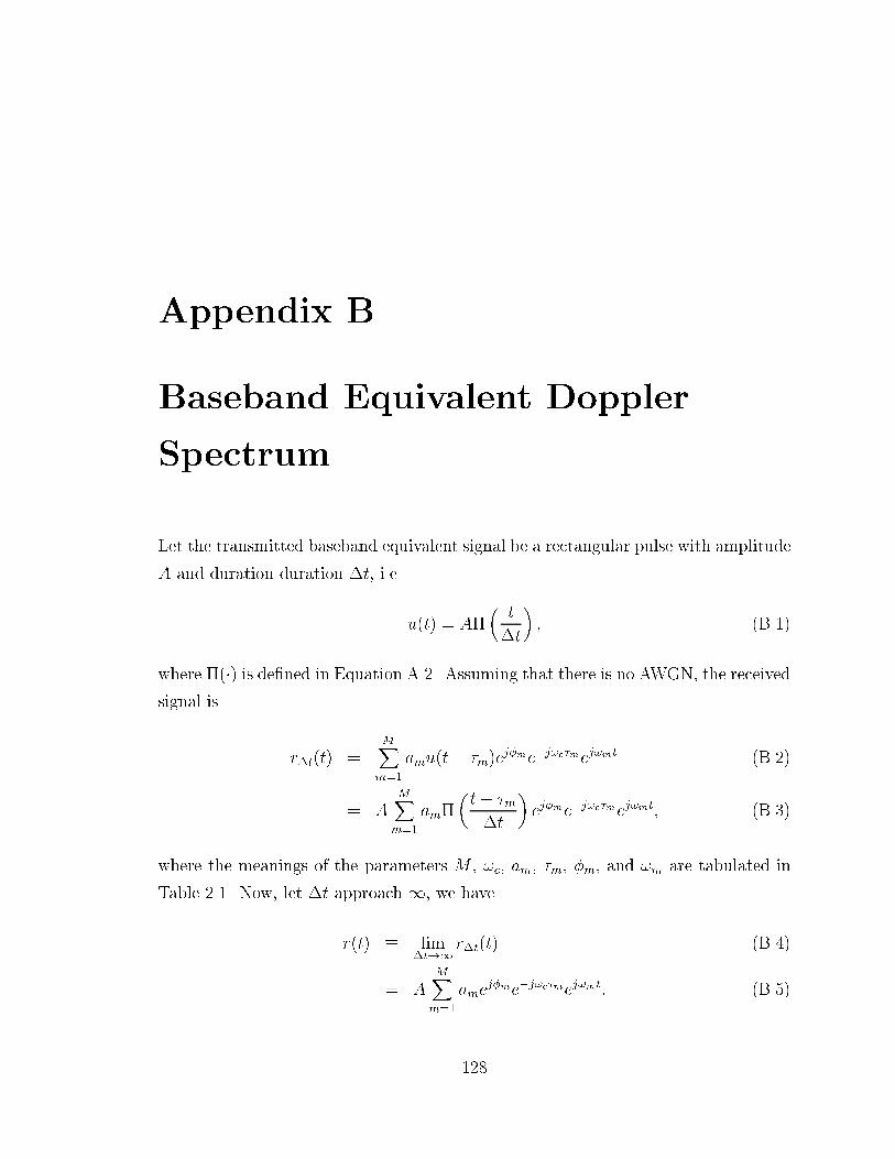
Appendix B
Baseband Equivalent Doppler
Spectrum
Let the transmitted baseband equivalent signal be a rectangular pulse with amplitude
A and duration duration �t, i.e.
u(t) = A�
�t
�t
�; (B.1)
where �(�) is de�ned in Equation A.2. Assuming that there is no AWGN, the received
signal is
r�t(t) =MX
m=1
amu(t� �m)ej�me�j!c�mej!mt (B.2)
= AMX
m=1
am�
�t� �m
�t
�ej�me�j!c�mej!mt; (B.3)
where the meanings of the parameters M , !c, am, �m, �m, and !m are tabulated in
Table 2.1. Now, let �t approach 1, we have
r(t) � lim�t!1
r�t(t) (B.4)
= AMX
m=1
amej�me�j!c�mej!mt: (B.5)
128
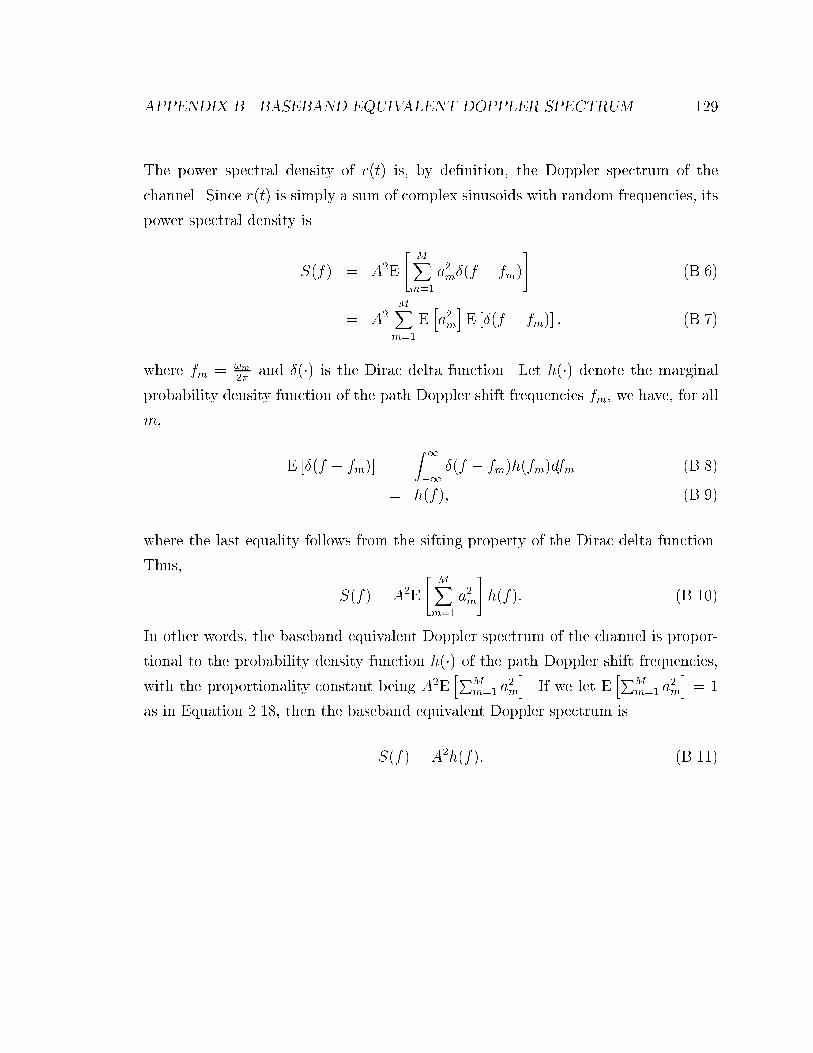
APPENDIX B. BASEBAND EQUIVALENT DOPPLER SPECTRUM 129
The power spectral density of r(t) is, by de�nition, the Doppler spectrum of the
channel. Since r(t) is simply a sum of complex sinusoids with random frequencies, its
power spectral density is
S(f) = A2E
"MX
m=1
a2m�(f � fm)
#(B.6)
= A2MX
m=1
Eha2m
iE [�(f � fm)] ; (B.7)
where fm = !m
2�and �(�) is the Dirac delta function. Let h(�) denote the marginal
probability density function of the path Doppler shift frequencies fm, we have, for all
m,
E [�(f � fm)] =
Z 1
�1�(f � fm)h(fm)dfm (B.8)
= h(f); (B.9)
where the last equality follows from the sifting property of the Dirac delta function.
Thus,
S(f) = A2E
"MX
m=1
a2m
#h(f): (B.10)
In other words, the baseband equivalent Doppler spectrum of the channel is propor-
tional to the probability density function h(�) of the path Doppler shift frequencies,
with the proportionality constant being A2EhP
M
m=1 a2m
i. If we let E
hPM
m=1 a2m
i= 1
as in Equation 2.18, then the baseband equivalent Doppler spectrum is
S(f) = A2h(f): (B.11)

Appendix C
The Least-Squares Lattice DFE
The least-squares lattice (LSL) DFE used in this dissertation was proposed by Ling
and Proakis[39, 40]. A block diagram of a LSL DFE with Nf taps in the feedforward
�lter and Nb taps in the feedback �lter is shown in Figure C.1. Assuming that Nf �Nb, the LSL DFE consists of (Nf �Nb � 1) \feedforward" stages, one \transitional"
stage, and Nb � 1 feedback stages. The feedforward stages are multi-channel LSL
stages[41] with dimensionality K, where the integer K is the number of samples
taken per symbol-period. The feedback stages are multi-channel LSL stages with
dimensionality K + 1. The transitional stage is a special stage that serves as the
interface between the K-dimensional feedforward stages and (K + 1)-dimensional
feedback stages. The inputs to the DFE are the sampled received signal y(t) and the
transmitted symbol (previous decision) x(t). This algorithm minimizes the weighted
square error (WSE) which is de�ned in Chapter 3 and repeated here for convenience1:
JNf�1(t) =tX
j=0
�t�j jx̂(j; t)� x(j)j2 ; (C.1)
In Equation C.1, the \forgetting factor" � is a positive real number less than but close
to 1, and x̂(j; t) is the estimate of the transmitted symbol x(j) obtained using the
�lter coe�cients of time t. The output of the LSL DFE is an estimate x̂(t) = x̂(t; t�1)
1All quantities in this appendix are discrete-time signals. Subscripts are used as order indices,
and parenthetic arguments are used as time indices. m and t are integers in all equations.
130

APPENDIX C. THE LEAST-SQUARES LATTICE DFE 131
+
+ +
+ + + +
+ ++ + + + +
N bN f- -1 N bN f
- N bN f- +1 N f-1
+ +
+
f0(t)
0(t)b
e (t)1D
21f1(t)
1(t)b
f2(t)
2(t)b
x (t)
e (t)2 e (t)3
y(t)
x(t)
(a)
+
+
f (t)m-1
b (t)m-1
f (t)m
b (t)m
D
(b)
Figure C.1: (a) The block diagram of a LSL DFE. Matrix weights are not explicitly
shown. The block labeled \D" denotes a unit-sample delay; (b) The block diagram of
a LSL stage. Matrix weights are not explicitly shown. The block labeled \D" denotes
a unit-sample delay.

APPENDIX C. THE LEAST-SQUARES LATTICE DFE 132
of the transmitted symbol x(t).
The time- and order-update recursions for the LSL DFE are as follows.
Feedforward stages (1 � m � (Nf �Nb� 1)) and feedback stages ((Nf �Nb+1) �m � (Nf � 1)):
fm(t) = fm�1(t)�K�m(t� 1)R�b
m�1(t� 2)bm�1(t� 1) (C.2)
bm(t) = bm�1(t� 1)�Km(t� 1)R�fm�1(t� 1)fm�1(t) (C.3)
Km(t) = �Km(t� 1) + �m�1(t� 1)bm�1(t� 1)f�m�1(t) (C.4)
�m(t) = �m�1(t)� j�m�1(t)j2b�m�1(t)R�bm�1(t)bm�1(t) (C.5)
Rfm(t) = Rf
m�1(t)�K�m(t)R�b
m�1(t� 1)Km(t) (C.6)
= �Rfm(t� 1) + �m(t� 1)fm(t)f
�m(t) (C.7)
Rbm(t) = Rb
m�1(t� 1)�Km(t)R�fm�1(t)K
�m(t) (C.8)
= �Rbm(t� 1) + �m(t)bm(t)b
�m(t) (C.9)
x̂m(t) = x̂m�1(t) + k�m(t� 1)R�b
m�1(t� 1)bm�1(t) (C.10)
em(t) = x(t)� x̂m(t) (C.11)
= em�1(t)� k�m(t� 1)R�b
m�1(t� 1)bm�1(t) (C.12)
km(t) = �km(t� 1) + �m�1(t)bm�1(t)e�m�1(t) (C.13)
Jm(t) = Jm�1(t)� k�m(t� 1)R�b
m�1(t� 1)km(t� 1) (C.14)
Transitional stage (m = Nf �Nb):
f (1)m(t) = fm�1(t)�K�
m(t� 1)R�b
m�1(t� 2)bm�1(t� 1) (C.15)
b(1)m(t) = bm�1(t� 1)�Km(t� 1)R�f
m�1(t� 1)fm�1(t) (C.16)
b(2)m(t) = em�1(t� 1)� kb�
m(t� 1)R�f
m�1(t� 1)fm�1(t) (C.17)
fm(t) =
24 f (1)
m(t)
em(t� 1)
35 (C.18)
bm(t) =
24 f (1)m
(t)
b(2)m(t)
35 (C.19)
Km(t) = �Km(t� 1) + �m�1(t� 1)bm�1(t� 1)f�m�1(t) (C.20)

APPENDIX C. THE LEAST-SQUARES LATTICE DFE 133
�m(t) = �m�1(t)� j�m�1(t)j2b�m�1(t)R�bm�1(t)bm�1(t) (C.21)
Rfm(t) = �Rf
m(t� 1) + �m(t� 1)fm(t)f
�m(t) (C.22)
Rbm(t) = �Rb
m(t� 1) + �m(t)bm(t)b
�m(t) (C.23)
x̂m(t) = x̂m�1(t) + k�m(t� 1)R�b
m�1(t� 1)bm�1(t) (C.24)
em(t) = x(t)� x̂m(t) (C.25)
= em�1(t)� k�m(t� 1)R�b
m�1(t� 1)bm�1(t) (C.26)
km(t) = �km(t� 1) + �m�1(t)bm�1(t)e�m�1(t) (C.27)
kbm(t) = �kb
m(t� 1) + �m�1(t� 1)fm�1(t)e
�m�1(t� 1) (C.28)
Jm(t) = Jm�1(t)� k�m(t� 1)R�b
m�1(t� 1)km(t� 1) (C.29)
The initial and boundary conditions are as follows.
Boundary conditions (m = 0):
f0(t) = y(t) (C.30)
b0(t) = y(t) (C.31)
Rf0(t) =
tXn=0
�t�ny(n)y�(n) + �t�I (C.32)
=
8<: y(0)y�(0) + �I; t = 0;
�Rf0(t� 1) + y(t)y�(t); t > 0:
(C.33)
Rb0(t) = Rf
0(t) (C.34)
�0(t) = 1 (C.35)
x̂0(t) = 0 (C.36)
e0(t) = x(t) (C.37)
J0(t) =tX
n=0
�t�njx(n)j2 (C.38)
=
8<: jx(0)j2; t = 0;
�Jm(t� 1) + jx(t)j2; t > 0:(C.39)

APPENDIX C. THE LEAST-SQUARES LATTICE DFE 134
Initial conditions (t = �1; 0):
Rbm(�1) = �I (C.40)
fm(0) =
8>>><>>>:y(0); 0 � m � Nf �Nb � 1;24 y(0)x(0)
35 ; Nf �Nb � m � Nf � 1:
(C.41)
bm(0) =
8<: y(0); m = 0;
0; m 6= 0:(C.42)
Km(0) = 0 (C.43)
�m(0) = 1 (C.44)
Rfm(0) =
8>>><>>>:y(0)y�(0) + �I; 0 � m � Nf �Nb � 1;24 y(0)x(0)
35 h y�(0) x�(0)
i+ �I; Nf �Nb � m � Nf � 1:
(C.45)
Rbm(0) =
8<: y(0)y�(0) + �I; m = 0;
�I; m 6= 0:(C.46)
km(0) = 0 (C.47)
� is a small positive real number in the above equations. The dimensionalities of
the variables in the LSL DFE algorithm are tabulated in Table C.1.
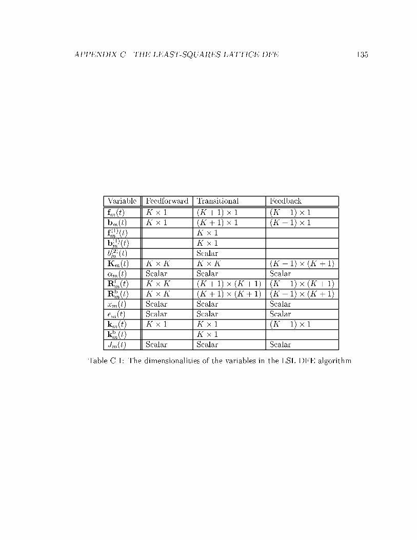
APPENDIX C. THE LEAST-SQUARES LATTICE DFE 135
Variable Feedforward Transitional Feedback
fm(t) K � 1 (K + 1)� 1 (K + 1)� 1
bm(t) K � 1 (K + 1)� 1 (K + 1)� 1
f (1)m(t) K � 1
b(1)m(t) K � 1
b(2)m(t) Scalar
Km(t) K �K K �K (K + 1)� (K + 1)
�m(t) Scalar Scalar Scalar
Rfm(t) K �K (K + 1)� (K + 1) (K + 1)� (K + 1)
Rbm(t) K �K (K + 1)� (K + 1) (K + 1)� (K + 1)
x̂m(t) Scalar Scalar Scalar
em(t) Scalar Scalar Scalar
km(t) K � 1 K � 1 (K + 1)� 1
kbm(t) K � 1
Jm(t) Scalar Scalar Scalar
Table C.1: The dimensionalities of the variables in the LSL DFE algorithm.

Appendix D
Optimality of MAP Selection Rule
In this Appendix, we will prove that the MAP selection rule described in Section 6.1
is optimal for a given SDDFE in the MAP sense, i.e. it maximizes the conditional
probability of making a correct �nal decision given all the outputs of the branch
DFE's.
Let1 z(l); l = 1; 2; : : : ; L, and x̂(l); l = 1; 2; : : : ; L, denote the branch DFE out-
puts and corresponding branch DFE decisions, respectively, where L is the number of
diversity branches. Furthermore, let x̂ denote the �nal decision for a given SDDFE us-
ing some selection rule. Conditioned on the branch DFE outputs z(l); l = 1; 2; : : : ; L,
we have
x̂ = x̂(l) with probability p(l) (D.1)
where
p(l) = Probhbranch l is selectedjz(1); z(2); : : : ; z(L)
i: (D.2)
Note that p(l) is a function of z(1); z(2); : : : ; z(L). Hence,
1Here we will omit the time index k since it is understood that selection is done on a symbol-by-
symbol basis.
136
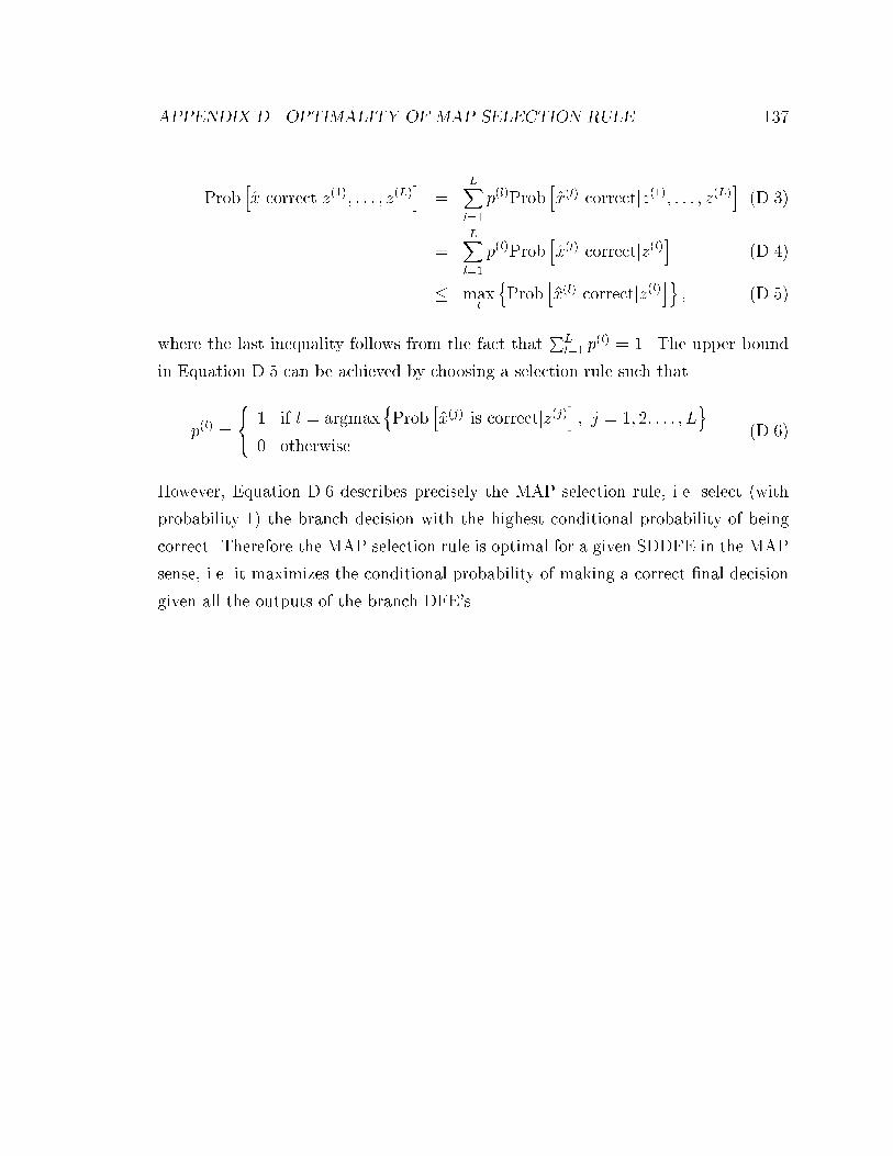
APPENDIX D. OPTIMALITY OF MAP SELECTION RULE 137
Probhx̂ correctjz(1); : : : ; z(L)
i=
LXl=1
p(l)Probhx̂(l) correctjz(1); : : : ; z(L)
i(D.3)
=LXl=1
p(l)Probhx̂(l) correctjz(l)
i(D.4)
� maxl
nProb
hx̂(l) correctjz(l)
io; (D.5)
where the last inequality follows from the fact thatP
L
l=1 p(l) = 1. The upper bound
in Equation D.5 can be achieved by choosing a selection rule such that
p(l) =
8<:
1 if l = argmaxnProb
hx̂(j) is correctjz(j)
i; j = 1; 2; : : : ; L
o0 otherwise.
(D.6)
However, Equation D.6 describes precisely the MAP selection rule, i.e. select (with
probability 1) the branch decision with the highest conditional probability of being
correct. Therefore the MAP selection rule is optimal for a given SDDFE in the MAP
sense, i.e. it maximizes the conditional probability of making a correct �nal decision
given all the outputs of the branch DFE's.

Bibliography
[1] W. C. Jakes, Microwave Mobile Communications, IEEE Press, 1994.
[2] D. C. Cox, R. R. Murray, and A. W. Norris, \Measurements of 800 MHz Radio
Transmission into Buildings with Metallic Walls," Bell System Technical Journal,
Vol. 62, pp. 2695�2717, November 1983.
[3] D. C. Cox, R. R. Murray, and A. W. Norris, \800 MHz Attenuation Mea-
sured In and Around Suburban Houses," Bell System Technical Journal, Vol. 63,
pp. 921�954, July-August 1984.
[4] R. J. C. Bultitude and G. K. Bedal, \Propagation Characteristics on Microcellu-
lar Urban Mobile Radio Channels at 910 MHz," IEEE Journal on Selected Areas
in Communications, Vol. 7, No. 1, pp. 31�39, January 1989,
[5] T. S. Rappaport, \Characterization of UHF Multipath Radio Channels in Fac-
tory Buildings," IEEE Transactions on Antennas and Propagation, Vol. 37,
No. 8, pp. 1058�1069, August 1989.
[6] D. C. Cox, \Universal Digital Portable Radio Communications," IEEE Proceed-
ings, Vol 75, No. 4, pp. 436�477, April 1987.
[7] T. S. Rappaport, Wireless Communications: Principles and Practice, Prentice
Hall, New Jersey, 1996.
[8] D. C. Cox, \Delay Doppler Characteristics of Multipath Propagation at 910 MHz
in a Suburban Mobile Radio Environment," IEEE Transactions on Antennas and
Propagation, Vol. 20, No. 5, pp 625�635, September 1972.
138

BIBLIOGRAPHY 139
[9] D. C. Cox and R. P. Leck, \Distributions of Multipath Delay Spread and Average
Excess Delay for 910-MHz Urban Mobile Radio Paths," IEEE Transactions on
Antennas and Propagation, Vol. 23, No. 2, pp. 206�213, March 1975.
[10] D. C. Cox and R. P. Leck, \Correlation Bandwidth and Delay Spread Multi-
path Propagation Statistics for 910-MHz Urban Mobile Radio Channels," IEEE
Transactions on Communications, Vol. 23, No. 11, pp. 1271�1280, November1975.
[11] D. C. Cox, \Multipath Delay Spread and Path Loss Correlation for 910-MHz
Urban Mobile Radio Propagation," IEEE Transactions on Vehicular Technology,
Vol. 26, No. 4, pp. 340�344, November 1977.
[12] T. S. Rappaport, S. Y. Seidel and R. Singh, \900-MHz Multipath Propagation
Measurements for U.S. Digital Cellular Radiotelephone," IEEE Transactions on
Vehicular Technology, Vol. 39, No. 2, pp. 132�139, May 1990.
[13] S. Y. Seidel et. al., \Path Loss, Scattering, and Multipath Delay Statistics in Four
European Cities for Digital Cellular and Microcellular Radiotelephone," IEEE
Transactions on Vehicular Technology, Vol. 40, No. 4, pp. 721�730, November1991.
[14] J. B. Andersen, T. S. Rappaport, and S. Yoshida, \Propagation Measurements
and Models for Wireless Communications Channels," IEEE Communications
Magazine, pp. 42�49, January 1995.
[15] D. M. J. Devasirvatham, \Time Delay Spread Measurements of Wideband Radio
Signals Within a Building," Electronics Letters, Vol. 20, No. 23, pp. 950�951,November 8, 1984.
[16] D. M. J. Devasirvatham, \Time Delay Spread and Signal Level Measurements
of 850 MHz Radio Waves in Building Environments," IEEE Transactions on
Antennas and Propagation, Vol. 32, NO 11, pp. 1300�1305, November 1986.
BIBLIOGRAPHY 140
[17] D. M. J. Devasirvatham, \A Comparison of Time Delay Spread and Signal Level
Measurements Within Two Dissimilar O�ce Buildings," IEEE Transactions on
Antennas and Propagation, Vol. 35, No. 3, pp.319�324, March 1987.
[18] , A. A. M. Saleh and R. A. Valenzuela, \A Statistical Model for Indoor Multipath
Propagation," IEEE Journal on Selected Areas in Communications, Vol. 5, No. 2,
pp. 128�137, February 1987.
[19] D. M. J. Devasirvatham, \Radio Propagation Studies in a Small City for
Universal Portable Communications," IEEE Vehicular Technology Conference,
pp. 100�104, June 1988.
[20] D. M. J. Devasirvatham et. al., \Time Delay Spread Measurements at 850 MHz
and 1.7 GHz Inside a Metropolitan O�ce Building," Electronics Letters, Vol. 25
No. 3, pp. 194�195, February 2, 1989.
[21] D. M. J. Devasirvatham et. al., \Radio Propagation Measurements at 850 MHz,
1.7 GHz and 4 GHz Inside Two Dissimilar O�ce Buildings," Electronics Letters,
Vol. 26 No. 7, pp. 445�447, March 29, 1990.
[22] D. M. J. Devasirvatham et. al., \Multi-Frequency Radiowave Propagation Mea-
surements in the Portable Radio Environment," 1990 IEEE International Con-
ference on Communications, pp. 335.1.1�335.1.7, April 1990.
[23] D. M. J. Devasirvatham et. al. \Multi-Frequency Propagation Measurements and
Models in a Large Metropolitan Commercial Building for Personal Communica-
tions," 1991 IEEE Symposium on Personal, Indoor and Mobile Communications,
September 1991.
[24] D. M. J. Devasirvatham et. al., \Two-Frequency Radiowave Propagation Mea-
surements in Brooklyn," 1992 IEEE International Conference on Universal Per-
sonal Communications, September 1992.
[25] H. Hashemi, \Impulse Response Modeling of Indoor Radio Propagation Chan-
nels," IEEE Journal on Selected Areas in Communications, Vol 11, No. 7,
pp. 967�978, September 1993.
BIBLIOGRAPHY 141
[26] J. C.-I. Chuang, \The E�ects of Time Delay Spread on Portable Radio Commu-
nications Channels with Digital Modulation," IEEE Journal on Selected Areas
in Communications, Vol. 5, No. 5, pp. 879�889, June 1987.
[27] J. G. Proakis, Digital Communications, 3rd Edition, McGraw-Hill, 1995.
[28] A. B. Carlson, Communication Systems: An Introduction to Signals and Noise
in Electrical Communication, 3rd Edition, McGraw-Hill, 1986.
[29] Y. Lee and D. C. Cox, \Multiple Decision Delay DFE for Short-Burst Indoor
Wireless Data Communications," IEEE International Conference on Universal
Personal Communications, October, 1997.
[30] R. W. Lucky, \Automatic Equalization for Digital Communications," Bell Sys-
tem Technical Journal, Vol. 44, pp. 547�588, April 1965.
[31] R. W. Lucky, \Techniques for Adaptive Equalization of Digital Communica-
tions," Bell System Technical Journal, Vol. 45, pp. 255�286, February 1966.
[32] J. G. Proakis and J. H. Miller, \Adaptive Receiver for Digital Signaling Through
Channels with Intersymbol Interference," IEEE Transactions on Information
Theory, Vol. 15, pp. 484�497, July 1969.
[33] S. U. H. Qureshi, \Adaptive Equalization," IEEE Proceedings, Vol. 53,
pp. 1349�1387, September 1985.
[34] E. A. Lee and D. G. Messerschmitt, Digital Communication, Boston: Kluwer
Academic Publishers, 1988, pp. 344�345.
[35] S. Ariyavisitakul and L. J. Greenstein, \Reduced-Complexity Equalization Tech-
niques for Broadband Wireless Channels," IEEE International Conference on
Universal Personal Communications, September, 1996.
[36] P. A. Voois et. al., \The E�ect of Decision Delay in Finite-Length Decision
Feedback Equalization," IEEE Transactions on Information Theory, Vol. 42,
No. 2, pp.618�621, March 1996.

BIBLIOGRAPHY 142
[37] N. Al-Dhahir et al. \E�cient Computation of the Delay-Optimized Finite
length MMSE-DFE," IEEE Transactions on Signal Processing, Vol. 44 No. 5,
pp. 1288�1292, May 1996.
[38] S. S. Haykin, Adaptive Filter Theory, 3rd Edition, Englewood Cli�s, NJ: Prentice
Hall, 1996.
[39] F. Ling and J. G. Proakis, \Adaptive Lattice Decision-Feedback Equalizers and
Their Application on Fading Dispersive Channels," 1983 IEEE International
Conference on Communications, pp. C8.2.1�C8.2.5, June 1983.
[40] F. Ling and J. G. Proakis, \Adaptive Lattice DFEs { Their Performance and
Application to Time-Variant Multipath Channels," IEEE Transactions on Com-
munications, Vol. COM-33, pp. 348�356, April 1985.
[41] F. Ling and J. G. Proakis, \A Generalized Multichannel Least Squares Lat-
tice Algorithm Based on Sequential Processing Stages," IEEE Transactions on
Acoustics, Speech, and Signal Processing, Vol. 32, No. 2, pp. 381�389, April1984.
[42] T. Kailath and B. Hassibi, State Space Estimation Theory, Stanford University,
1996.
[43] Y. Lee and D. C. Cox, \MAP Selection Diversity DFE for Indoor Wireless Data
Communications," Proceedings of IEEE International Conference on Universal
personal Communications, Vol. 1, pp.115�119, September-October, 1996.
[44] P. K. Shukla et. al., \Channel-Estimation-Based adaptive DFE for Fading Mul-
tipath Radio Channels," IEE Proceedings-I, Vol. 138, No. 6, pp. 525�543, De-cember 1991.
[45] R. A. Ziegler et. al., \Nonrecursive Adaptive DFE from Channel Estimates,"
Proceedings of IEEE Global Communications Conference, pp. 600�603, 1992.

BIBLIOGRAPHY 143
[46] Y. Lee and D. C. Cox, \Adaptive Equalization with Regularization for In-
door Wireless Data Communications," IEEE Global Communications Confer-
ence, November 1997.
[47] C. L. Zahm, \Applications of Adaptive Arrays to Suppress Strong Jammers
in the Presence of Weak Signals," IEEE Transactions on Aerospace Electronic
Systems, Vol. 9, pp. 260�271, March 1973.
[48] G. Ungerboeck, \Fractional Tap-Spacing Equalizer and Consequences for Clock
Recovery in Data Modems," IEEE Transactions on Communications, Vol. 24,
pp. 856�864, August 1976.
[49] J. Treichler, The Spectral Line Enhancer, Ph.D. Dissertation, Stanford Univer-
sity, May 1977.
[50] R. D. Gitlin et. al., \The Tap-Leakage Algorithm: An Algorithm for the Stable
Operation of a Digitally Implemented, Fractionally Spaced Adaptive Equalizer,"
Bell System Technical Journal, Vol. 61, No. 8, pp. 1817�1839, October 1982.
[51] J. M. Cio�, \Limited-Precision E�ects in Adaptive Filtering," IEEE Transac-
tions on Circuits and Systems, Vol. 34, No. 7, pp. 821�833, July 1987.
[52] P. S. Bednarz, Decision Feedback Detection for the Digital Magnetic Storage
Channel, Ph.D. Dissertation, Stanford University, 1997.
[53] S. Qureshi, \Adjustment of the Position of the Reference Tap of an Adaptive
Equalizer," IEEE Transactions on Communications, Vol. 21, pp.1046�1052,September 1973.
[54] A. Valdovinos et. al., \Analysis of Diversity and Equalization Techniques Ap-
plied to M-QAM Digital Mobile Radio Systems," Proceedings of IEEE Vehicular
Technology Conference, pp. 957�961, June 1994.
[55] J. D. Gibson, ed., \The Mobile Communications Handbook," CRC Press, 1996.
BIBLIOGRAPHY 144
[56] S. A. Bergmann and H. W. Arnold, \Polarization Diversity in The Portable
Communications Environment," Electronic Letters, pp. 609�610, May 22, 1986.
[57] D. C. Cox, \Introduction to Wireless Communications { EE276 Course Reader,"
Stanford University, 1997.
[58] T. A. Freeburg, \Enabling Technologies for In-Building Network Communica-
tions { Four Technical Challenges and Four Solutions," IEEE Transactions on
Vehicular Technology, Vol. 29, No. 4, pp.58�64, 1991.
[59] P. Monsen, \Theoretical and Measured Performance of a DFE Modem on a
Fading Multipath Channel," Vol. 25, No. 10, pp.1144�1153, October 1977.
[60] P. Monsen, \MMSE Equalization of Interference on Fading Diversity Channels,"
IEEE Transactions on Communications, Vol. 32, No. 1, pp. 5�12, January 1984.
[61] Q. Liu et. al., \Performance of Decision-Feedback Equalizers with Dual Antenna
Diversity," Proceedings of IEEE Vehicular Technology Conference, pp. 637�640,May 1993.
[62] H. Ishikawa and H. Kobayashi, \Selection Diversity With Decision-Feedback
Equalizer," Proceedings of IEEE Vehicular Technology Conference, Vol. 2,
pp.962�966, June 1994.
[63] S. Venkataraman et. al., \Filter Structures for Equalization and Diversity Com-
bining in Wireless Communications," Proceedings of IEEE International Con-
ference on Universal Personal Communications, pp. 204�209, October 1994.
[64] M. Serizawa et. al., \Tracking Ability of Decision Feedback Equalizer for Time-
Varying Channel Characteristics," Electronics and Communications in Japan,
Part 1 (Communications), Vol. 78, No. 9, pp. 103�113, September 1995.
[65] B. Widrow and S. Stearns, Adaptive Signal Processing, Englewood Cli�s, N.J.:
Prentice-Hall, 1985.
BIBLIOGRAPHY 145
[66] S. Lin and D. Costello, Error Control Coding: Fundamentals and Applications,
Englewood Cli�s, N.J.: Prentice-Hall, 1983.
[67] K. Pahlavan and A. H. Levesque, \Wireless Data Communications," IEEE Pro-
ceedings, Vol. 82, No. 9, pp.1398�1430, September 1994.
[68] M. Luise and R. Reggiannini, \Carrier Frequency Recovery in All-Digital
Modems for Burst-Mode Transmissions," IEEE Transactions on Communica-
tions, Vol. 43, No. 2/3/4, pp. 1169�1178, February/March/April, 1995.