AD_________________

AWARD NUMBER: DAMD17-00-1-0291 TITLE: A Training Program in Breast Cancer Research Using NMR Techniques PRINCIPAL INVESTIGATOR: Paul C. Wang, Ph.D. CONTRACTING ORGANIZATION: Howard University Washington, DC 20059 REPORT DATE: July 2006 TYPE OF REPORT: Final PREPARED FOR: U.S. Army Medical Research and Materiel Command Fort Detrick, Maryland 21702-5012 DISTRIBUTION STATEMENT: Approved for Public Release; Distribution Unlimited The views, opinions and/or findings contained in this report are those of the author(s) and should not be construed as an official Department of the Army position, policy or decision unless so designated by other documentation.

REPORT DOCUMENTATION PAGE Form Approved

OMB No. 0704-0188 Public reporting burden for this collection of information is estimated to average 1 hour per response, including the time for reviewing instructions, searching existing data sources, gathering and maintaining the data needed, and completing and reviewing this collection of information. Send comments regarding this burden estimate or any other aspect of this collection of information, including suggestions for reducing this burden to Department of Defense, Washington Headquarters Services, Directorate for Information Operations and Reports (0704-0188), 1215 Jefferson Davis Highway, Suite 1204, Arlington, VA 22202-4302. Respondents should be aware that notwithstanding any other provision of law, no person shall be subject to any penalty for failing to comply with a collection of information if it does not display a currently valid OMB control number. PLEASE DO NOT RETURN YOUR FORM TO THE ABOVE ADDRESS. 1. REPORT DATE (DD-MM-YYYY)01-07-2006

2. REPORT TYPEFinal

3. DATES COVERED (From - To)1 Jul 2000 – 30 Jun 2006

4. TITLE AND SUBTITLE

5a. CONTRACT NUMBER

A Training Program in Breast Cancer Research Using NMR Techniques 5b. GRANT NUMBER DAMD17-00-1-0291

5c. PROGRAM ELEMENT NUMBER

6. AUTHOR(S)

5d. PROJECT NUMBER

Paul C. Wang, Ph.D. 5e. TASK NUMBER

E-Mail: pwang@howard.edu 5f. WORK UNIT NUMBER

7. PERFORMING ORGANIZATION NAME(S) AND ADDRESS(ES)

8. PERFORMING ORGANIZATION REPORT NUMBER

Howard University Washington, DC 20059

9. SPONSORING / MONITORING AGENCY NAME(S) AND ADDRESS(ES) 10. SPONSOR/MONITOR’S ACRONYM(S)U.S. Army Medical Research and Materiel Command

Fort Detrick, Maryland 21702-5012 11. SPONSOR/MONITOR’S REPORT NUMBER(S) 12. DISTRIBUTION / AVAILABILITY STATEMENT Approved for Public Release; Distribution Unlimited

13. SUPPLEMENTARY NOTES

14. ABSTRACT This is a six year training program in breast cancer research using NMR techniques. This program has supported seven predoctoral students and five postdoctoral students. All the trainees have learned the theory and instrumentation of MRI. They have been actively involved in one of the seven research projects: (1) NMR studies of phosphorus metabolites of breast cancer cells using an improved cell perfusion system (2) Segmentation of mammographic masses (3) Establishment of an image database for computer-aided-diagnosis (CAD) research development (4) F19 NMR detection of trifluoperazine crossing Blood-Brain-Barrier through Pgp modulation (5) Tumor-targeted MR Contrast Enhancement by Anti-transferrin Receptor scFv-Immunoliposome Nanoparticles (6) MRI and histological correlations of cortical brain volumes in APP/PS1 mice (7) Enhanced molecular imaging with fused optical and MRI images. The trainees have attended the weekly seminars in the Cancer Center and also attended a special NMR seminar series in the Department of Radiology. Eight papers have been published and 16 abstracts have been presented in the national and international meetings. Five grants including a USAMRMC postdoctoral award have received.

15. SUBJECT TERMSTraining, Nuclear Magnetic Resonance, Breast Cancer

16. SECURITY CLASSIFICATION OF:

17. LIMITATION OF ABSTRACT

18. NUMBER OF PAGES

19a. NAME OF RESPONSIBLE PERSONUSAMRMC

a. REPORT U

b. ABSTRACTU

c. THIS PAGEU

UU

86

19b. TELEPHONE NUMBER (include area code)

Standard Form 298 (Rev. 8-98)Prescribed by ANSI Std. Z39.18

Table of Contents

Cover…………………………………………………………………………………… 1 SF 298……………………………………………………………………………..…… 2 Table of Contents………………………………………………………………..…… 3 Introduction……………………………………………………………….………….... 4 Body……………………………………………………………………………………. 4 Key Research Accomplishments………………………………………….……… 9 Reportable Outcomes………………………………………………………………. 10 Conclusions………………………………………………………………………….. 14 Abbreviations………………………………………………………………………… 15 Appendices…………………………………………………………………………… 16

3

A Training Program In Breast Cancer Research Using NMR Techniques I. INTRODUCTION

The purpose of this proposal was to develop a research training program in breast cancer research at Howard University Cancer Center utilizing nuclear magnetic resonance (NMR) imaging and spectroscopy techniques. This program was a multidisciplinary consortium of five departments including College of Medicine MD/PHD program, Radiology, Radiation Oncology, Biology and Electrical Engineering. Through this program, we have trained seven predoctoral students and five postdoctoral students in six years. The predoctoral students were either from the MD/PhD program or from the Department of Electrical Engineering. The MD/PhD program is a seven-year program in which the students do research in the Department of Biochemistry and Molecular Biology. The postdoctoral fellows were from a medical or physical science background with strong interests in breast cancer research. All the students have participated in the research projects conducted in the Biomedical NMR Laboratory. In the later years of the program, the postdoctoral fellows were encouraged to develop their own research projects. Although the research component of the training was focused on NMR applications in breast cancer research, the trainees received a broad exposure to other aspects of breast cancer research through a rigorous curriculum, interactions with faculty, and participation in seminars and other research activities in the Howard University Cancer Center. The program was flexible and tailored to the trainees’ backgrounds to ensure the trainees receive a well-rounded education. This program has accomplished its goal to provide an educational and research opportunity to promising young African-American students to become productive breast cancer researchers. II. BODY Statement of Work (All the tasks in the Statement of Work have completed). For Predoctoral Students Year 1: • Introduction to the Biomedical NMR Laboratory and Cancer Center. Meeting with mentors

to learn the on-going breast cancer projects (months 1 - 3) • Learn NMR instruments (months 4 -12) • Start departmental course work with the respective department (months 4 - 12) • Seminar presentation by the student each semester (months 4 - 12) • Clinical preceptorship one half day per week (months 4 - 12) • Report to MD/PhD committee and respective department on research progress (month 12) Year 2-3: • Take departmental comprehensive exams (months 13 - 15) • Submit a five page pre-proposal 30 days before taking comprehensive exam (months 13-15) • Write an expanded research proposal and defend the proposal (months 16-18) • Once the student has passed the written and oral comprehensive exams, the student is

qualified as a Ph.D. candidate

4

• Select a thesis committee (month 18) • Start thesis project (month 18) • Report to MD/PhD committee and respective department on research progress each semester

(months 18 - 36) • Clinical preceptorship one half day per week (months 13 - 36) Year 4: • Conclude the thesis project and write up thesis (months 37 - 42) • Thesis defense and writing of scientific papers for publication (month 43 - 48) For Postdoctoral Students: Year 1: • Introduction to the Biomedical NMR Laboratory at the Cancer Center. Meeting with

mentors to learn the on-going projects (months 1-2) • Participate in weekly Cancer Center Seminars (months 1-2) • Learn to use three NMR instruments in the laboratory (months 1-12) • Take cell biology course taught by Dr. Bremner and NMR course taught by Dr. Wang

(months 3-12) • Select an on-going project and start to get involved with the research project (months 4-12) Year 2: • Participate in weekly Cancer Center Seminars (months 13-24) • Organize weekly research group meeting (months 13-24) • Continue research project (month 13-24) • Present progress report to the Executive Committee (months 18 and 24) • Clinical preceptorship one half day per week (months 13-24) Years 3-4: • Select a new research project approved by the Executive Committee (months 25-27) • Clinical preceptorship one half day per week (months 25-48) • Conduct the new research project (months 28-48) • Present progress report to the Executive Committee once every six months (months 28-48) • Present research results to the Cancer Center faculty and National Meeting • Write scientific papers Students trained in this program: Pre-doctoral students: (graduate program, current position) Emmanuel Agwu (MD/PhD, Biochemistry, internal medicine resident at HUH) O’tega Ejofodomi (Electrical Engineering, graduate student at HU) Lisa Kinnard (Electrical Engineering, researcher at FDA) Raymond Malveaux (medical student at Howard University) Armand Oei (Biology, student at New England School of Optometry) Shani Ross (Electrical Engineering, graduate student at U Michigan) Furia Thomas (Electrical Engineering, graduate student at Catholic University)

5

Postdoctoral students: (current position) Yusuf Ali, MD (radiology resident at Howard University Hospital) Ercheng Li, PhD (staff, Chemistry Department, Georgetown University) Huafu Song, MS (Engineer, NMR industry) Jianwei Zhou, PhD (assistant professor, Quiyang Normal University, China) Renshu Zhang, MD (research associate, Department of Radiation Oncology, HUH) Research Projects In this training grant, students have participated in seven research projects listed as follows: (1) NMR Studies of Phosphorus Metabolites of Breast Cancer Cells Using an Improved Cell Perfusion System P31 NMR has been used to study the high energy phosphorus metabolites in tumors. It can be used to monitor the effectiveness of cancer treatment. Since the NMR signals of the phosphorus metabolites in cells are weak and the NMR study usually are long. During the long data acquisition time, the cancer cells need to be maintained in a good living environment. In this project, we developed an improved NMR cell-perfusion system, which was used to study the phosphorus metabolites of breast cancer cells for an extended period. The improved perfusion system is driven by a peristaltic pump. The portion of the system before the pump is under negative pressure, and the portion after the pump is under positive pressure. This design helps the removal of air bubbles trapped in the perfusion medium and avoid the degradation of the quality of NMR spectrum. Using this perfusion system, NMR study of the breast cancer cells can be extended for more than a week not hours as it used to be. The P31 NMR spectrum of the wild type MCF7 breast cancer cells shows three distinct phases, which reflect the proliferation of the cells. Study of oxygenation of the agarose-encased cells in this perfusion system suggests that the cells utilized aerobic respiration. The ability for this perfusion system to maintain cells viable for more than a week allowed us to determine the longitudinal relaxation times (T1 values) of the P31 metabolites of MCF7/WT cells in vitro. A progressive saturation recovery NMR technique was used for T1 measurement. Accurate T1 values are crucial in designing P31 MRS studies. This study has demonstrated that the long time bubble-free NMR cell perfusion system could be a useful tool for in vitro breast cancer research. (2) Segmentation of Mammographic Masses

Mammography combined with a clinical examination is a standard method used for the detection and diagnosis of breast cancer. However, mammography alone can produce a high percentage of false positives. A computer-aided diagnostic (CADx) system can serve as a more accurate clinical tool for the radiologist, consequently lowering the rate of missed breast cancer and ultimately lowering morbidity and mortality. Breast cancer can exist not only in the form of masses, but also in the forms of microcalcifications, asymmetric density, and architectural distortion. These abnormalities can be seen using imaging techniques such as mammography, ultrasound and magnetic resonance imaging (MRI). Breast images have different appearances based upon their amounts of fibroglandular and fatty tissue. Fibroglandular tissue usually consists of a combination of breast glands (lobules), ducts, and surrounding fibrosis (fibrous connective tissue and scarring). It appears denser or brighter than fatty tissue on mammograms

6

due to its higher x-ray attenuation. The diseased tissue usually also becomes denser over time. Masses can have unclear borders and are sometimes overlapped with glandular tissue in mammograms; therefore, the radiologists can overlook them during their search for suspicious areas. Proper segmentation to include the shape and boundary characteristics is an essential step in aiding the computer for the analysis and malignancy determination of the mass. While many CADx systems have been developed, the development of effective image segmentation algorithms for breast masses remains unsolved in this field, particularly in the cases where the breast tissue is dense. Since cancerous masses often appear to be light and have ill-defined borders, it is quite challenging for mammographers to extract them from surrounding tissue. It is even more difficult to automatically segment masses from dense tissue. In this study, a fully automated segmentation algorithm has been developed. It delineates the complete mass as with minimum normal structures in dense and mixed tissue mammograms. (3) Establishment of an Image Database for Computer-Aided-Diagnosis (CADx) Research

Development The success of CADx is based on the accuracy and completeness of the mammographic image database, of which the CADx extracts the features of different types of pathology. The current available mammographic image databases are all obtained from the Caucasian population. There are very few African American cases. It is well known that African American women generally have denser breasts. The appearance of mammograms from African American breast cancer patients may not be the same as those images from Caucasian breast cancer patients. Howard University Cancer Center has a well maintained cancer registry. It has more than 200 new African American breast cancer cases each year. We have digitized more than 5000 images from 260 patients’ records using a high resolution Kodak LS85 laser scanner. The database system and web-based search engine were developed using MySQL and PHP. The database has been evaluated by medical professionals and the experimental results obtained are promising with high image quality and fast access time. We have also developed an image viewing system, D-Viewer, to display these digitized mammograms. This viewer is coded in Microsoft Visual C++ and is intended to help medical professionals view and retrieve large data sets in near real time. Finally, we have developed an image content-based retrieval function for the database system in order to provide improved search capability for the medical professionals. (4) F19 NMR Detection of Trifluoperazine Crossing Blood-Brain-Barrier Through Pgp

Modulation Cancer patients are often treated with combination therapy for secondary symptoms such

as depression, and cardiopulmonary diseases. The potential for drug-drug interaction under these conditions is high. Such interactions may cause changes in the pharmacokinetics, especially for drugs with narrow therapeutic indices. These changes can alter efficacy and toxicity of the administered drugs. Drug-drug interactions may occur due to common metabolic pathways, but also due to interference at the P-glycoprotein (Pgp) level. Pgp, a nonspecific transport protein, is expressed constitutively at the blood-brain-barrier (BBB), intestine, kidney, liver, and in activated T-cells. Interaction at the blood-brain-barrier may occur if one of the two concomitantly administered drugs blocks Pgp thus allowing the other drug to retain in the brain or increase in brain uptake of therapeutic drugs. The potential for drug-drug interactions is not routinely studied at the Pgp level during drug development. Its presence is assumed only after unexpected clinical symptoms. We have shown using a dynamic NMR method based on

7

detection of a fluorinated drug, trifluoperazine (TFP), in the brain, in combinations with an immune suppressor, cyclosporin A to demonstrate drug penetration across blood-brain-barrier after Pgp modulation.

(5) Tumor-targeted MR Contrast Enhancement by Anti-transferrin Receptor scFv-

Immunoliposome Nanoparticles The development of improvements in MRI that would enhance sensitivity, thus leading to earlier detection of cancer and visualization of metastatic disease, is an area of intense exploration. In this study, we developed the cationic immunoliposome system that includes an anti-transferrin receptor single chain antibody fragment (TfRscFv) as the targeting molecule was used to encapsulate the MR contrast agent gadolinium (TfRscFv-Lip-GAD-d) for specific targeting to cancer cells and MR contrast enhancement. This system was evaluated for in vivo MR imaging in MDA-MB-435 breast cancer cells growing as solid tumor xenografts in athymic nude mice. The TfRscFv-Lip-GAD-d complex was administered intravenously at an encapsulated contrast agent. The MRI signal intensity of tumors was significantly enhanced compared to free contrast agent and the enhancement was closely related to the pathology of the tumors. These results indicate that this TfRscFv-Lip-GAD-d system significantly enhances the image contrast in solid tumors and is much superior to the contrast agent alone for identifying the tumor pathological features. This targeted immunoliposome system may serve as a powerful MR imaging probe for early detection and differential diagnosis of tumors. (6) MRI and Histological Correlations Of Cortical Brain Volumes In APP/PS1 Mice Quantitative analyses indicate that brain atrophy on ante-mortem neuroimages and post-mortem tissue strongly correlates with the severity of cognitive impairment in Alzheimer’s disease (AD). The absence of cortical atrophy in the age-matched, non-demented elderly suggests that volumetric studies of ante-mortem neuroimages may provide an early marker of AD in aging populations. In this study we used design-based stereology to quantify cortical volumes in double transgenic mice that deposit AD-type mutant ß-amyloid proteins (Aß) in cortical tissue. Spin-echo T1-weighted, high-resolution magnetic resonance imaging (MRI) was applied to the brain of male and female double transgenic mice aged 4-28 months of age that co-express AD-type mutations in amyloid precursor protein (APP) and presenilin-1 (PS-1), and, age-matched non-tg littermate controls (wild-type, WT). From a systematic-random series of coronal MRI images, total volumes of the hippocampal formation (VHF) and whole brain (Vbrain) were quantified by the Cavalieri-point counting method. The same sampling and estimation methods were used to quantify the same brain regions after perfusion and tissue processing. Strong correlations were found between VHF and Vbrain estimates from MRI images and histological sections. Agonal and tissue processing changes accounted for about 65 to 75% differences in cortical volumes between in situ and coverslipped sections. No differences were present in mean VHF or mean Vbrain for dtgAPP/PS1 compared to WT mice. These stereological studies of MRI neuroimages and postmortem tissue do not show cortical atrophy in association with widespread cortical deposition of AD-type amyloid plaques in aged dtg APP/PS1 mice, in contrast to the severe cortical atrophy in AD. Future studies with dtgAPP/PS1 mice will explore the possibility that high contrast ligands bound to mutant Aß proteins associated with amyloid plaques could facilitate early diagnosis of AD by ante-mortem neuroimaging. (7) Enhanced Molecular Imaging with Fused Optical and MRI Images

8

Improvement in molecular and cell biology techniques in recent years have had remarkable impact on our understanding of the cellular and molecular mechanisms of biological processes and the underlie development of diseases. Significant development have been made in noninvasive, high-resolution, in vivo imaging modalities such as positron emission tomography (PET), magnetic resonance imaging (MRI), and optical imaging (OI) for better diagnosis of patients, and imaging of cells and small animals of diseased models. In vivo molecular imaging, which utilizes these two fronts, opens up extraordinary opportunities for basic scientists and clinicians to study diseases, and in many cases, quantitatively at the molecular level. The early assessment of illness depends on anatomic and physiological changes of the disease, which are a late manifestation of the molecular changes that truly triggers the disease. Imaging early molecular changes at “predisease states” would be useful in patient care and management by allowing much earlier detection of the disease, designing more effective drugs, and evaluation of therapy. This research is to combine the strength of MRI and optical imaging modalities for better spatial and functional information in small animal imaging. The technique would be useful to evaluate targeting specificity of near infrared dye conjugated ligands in molecular imaging of tumor bearing animals. III. KEY RESEARCH ACCOMPLISHEMENTS Year 1 (2000-01)

• An improved NMR cell-perfusion system driven by peristaltic pump was constructed. This system totally eliminated the air bubbles from the perfusion medium.

• The cell viability study of the MCF-7 breast cancer cells was extended successfully from hours to more than a week.

Year 2 (2001-02) • Intravascular MRI contrast agent has been used to detect high blood flow, vascular

density, and capillary permeability of tumors. • Dynamic MRI contrast enhancement is an important parameter for tumor

characterization, and it correlates well with histopathological findings. • Using pixel aggregation and likelihood analysis techniques, the segmentation method can

delineate the tumor body as well as tumor peripheral regions covering typical mass boundaries and some speculation patterns.

Year 3 (2002-03) • We found that the maximum likelihood method in conjunction with fuzzy shadow

approach is an effective approach not only for segmenting masses in mammogram, but also for using its results to separate malignant and benign masses.

• We have demonstrated that cyclosporin A, an immune suppressor, enhances the drug penetration through the blood-brain-barrier.

Year 4 (2003-04) • A fully automated segmentation algorithm for Computer-Aided-Diagnosis has been

developed. It delineates the complete masses with minimum normal structures in dense and mixed tissue mammograms.

• Drug penetration of trifluoperazine through the blood-brain-barrier due to Pgp modulation was detected using a dynamic in vivo F19 NMR method.

9

• Utilizing a well maintained cancer registry at the Howard University Cancer Center, mammograms from more than 200 African American breast cancer patients were digitized to establish a breast cancer image database. It will be available on the Internet to the CADx software developers and researchers.

• Developed a TfR scFv-immunoliposome system to be used as a MR contrast agent delivery vehicle for improving affinity and specificity of contrast agent to tumor association.

Year 5 (2004-05) • An improved NMR cell-perfusion system was developed. It has been used to study the

phosphorus metabolites of breast cancer cell for an extended period longer than one week. Using this perfusion system, the T1 relaxation times of phosphorus metabolites were accurately measured.

• The image digitization of more than 1000 mammograms from 220 African American breast cancer patients has completed. This huge image database is available to be used in the further development of Computer-Aided-Diagnosis system.

• MRI contrast agent is incorporated into an anti-transferrin receptor single chain antibody (TfRsc) liposome nanoparticle for MRI molecular imaging. This significantly improves the image contrast between tumor and surrounding tissues. This improves the specificity of MRI imaging of tumor.

Year 6 (2005-06) • Based on the finished mammography database of 260 African American (40 more cases),

two previously supported students, Ms. Ross and Ms Ejofodomi wrote a paper entitled “A Mammography Database and View System for African American Patients”. The paper has been submitted to the Journal of Digital Imaging for publication. This huge image database is available to be used in the further development of Computer-Aided-Diagnosis system.

• A graduate student, Mr. Furia Thomas, has worked on a project for image fusion of MRI images and optical images. The MRI images provide detail anatomical information and the optical images provide functional information of the tissue. The greater imaging sensitivity of optical imaging technique can be complemented by the high resolution MRI images when these two images are fused together. Mr. Thomas has submitted an abstract entitled “Enhanced Molecular Imaging with Fused Optical and MRI Images” to the 28th IEEE Engineering in Medicine and Biology Conference Management System, July 2006.

• The PI has continued developing the nanosize cationic immunoliposome system that includes an anti-transferrin receptor single chain antibody fragment (TfRscFv) as the targeting molecule was used to encapsulate the MR contrast agent gadolinium-DTPA (TfRscFv-Lip-GAD-d) for specific targeting to cancer cells and MR image contrast enhancement. This system was evaluated for MR imaging of breast cancer cells in vitro as well as in vivo. The signal intensity of tumors was significantly enhanced compared to free contrast agent and the enhancement was closely related to the pathology of the tumors.

IV. REPORTABLE OUTCOMES Research

10

Reprints (Listed in the Appendices section)

1. Kinnard L, Lo S-C.B, Wang P, Freedman MT, Chouikha M, Separation of Malignant and Benign Masses in Mammography using Maximum-Likelihood Modeling and Neural Networks. Proc. of SPEI Vol 4684: 733-741, 2002.

2. Lo S-C.B, Li H, Wang Y, Kinnard L, Freedman M, A Multiple Circular Path Convolution Neural Network System for Detection of Mammographic Masses, IEEE Transactions on Medical Imaging, Vol 21, No 2 pp 150-158. 2002

3. Kinnard L, Lo S-C B, Wang PC, Freedman MT, Chouikha M, Automatic Segmentation of Mammographic Masses Using Fuzzy Shadow and Maximum-likelihood Analysis, Proc of IEEE Symposium on Biomedical Imaging (Cat 02EX608C): pp. 241-244, 2002.

4. Kinnard L, Lo S-C.B, Wang PC, Freedman MT, Chouikha M, Separation of Malignant and Benign Masses Using Image and Segmentation Features. Proc. of SPIE, 2003

5. Kinnard L, Lo SB, Makariou E, Osicka T, Wang PC, Freeman M, Chouikha M. Likelihood Function Analysis For Segmentation of Mammographic Masses For Various Margin Groups. Proc of IEEE Symposium on Biomedical Imaging. pp 113-116, 2004.

6. Liang XJ, Yin JJ, Zhou JW, Wang PC, Taylor B, Cardarelli C, Kozar M, Forte R, Aszalos A, Gottesman M. Changes in Biophysical Parameters of Plasma Membranes Influence Cisplatin Resistance of Sensitive and Resistant Epidermal Carcinoma Cells. Exp Cell Research 293:283-291, 2004.

7. Kinnard L, Lo SB, Makariou E, Osicka T, Wang P, Chouikha MF, Freedman MT. Steepest changes of a probability-based cost function for delineation of mammographic masses: A validation study. Med. Phys. 31(10):2796-2810, 2004.

8. Pirollo K, Dagata J, Wang PC, Freedman M, Vladar A, Fricke S, Ileva L, Zhou Q, Chang EH. A Tumor-Targeted Nanodelivery System to Improve Early MRI Detection of Cancer. J Mol Imaging 5(1):41-52, 2006.

Presentations

1. Zhou JW, Agwu CE, Li EC, Wang PC. An Improved NMR Perfusion System For Breast Cancer Cell Study. 42nd Experimental NMR Conference, March 11-16, 2001, Orlando, FL.

2. Ting P, Wang PC, Kinnard L, Herman MM, Cohn R. Early EEG and Diffusion MRI (dMRI) Changes in an Experimental Model of Severe Periventircular Leukomalacia (PVL). The Annual Pediatric Academic Societies Meetings, May 1-5, 2001, Baltimore, MD.

3. Agwu EC, Zhou JW, Sridhar R, Wang PC. An Improved NMR Perfusion System For Breast Cancer Cell Study. Association For Academic Minority Physicians 15th Annual Scientific Meeting, October 12-14, Washington, DC. 2001.

4. Zhang RS, Li EC, Ali YD, Song HF, Fan KJ, Pirollo KF, Chang EH, Wang PC. Dynamic Magnetic Resonance Imaging of Prostate Cancer in Mice. American Association for Cancer Research Conference, Molecular Imaging in Cancer: Linking Biology, Function, and Clinical Application In Vivo, January 23-27, 2002, Orlando, Fl.

5. Kinnard L, Lo S-C.B, Wang P, Freedman MT, Chouikha M, Separation of Malignant and Benign Masses in Mammography using Maximum-Likelihood Modeling and Neural Networks. SPEI Med Imaging, Feb. 2002, San Diego, CA.

6. Kinnard L, Lo S-C B, Wang PC, Freedman MT, Chouikha M. A Maximum-likelihood

11

Automated Approach to Breast Mass Segmentation. 2002 1st IEEE International Symposium on Biomedical Imaging: Macro to Nano, Washington, DC, July 7-10, 2002.

7. Kinnard L, Lo S-C B, Wang PC, Freedman MT, Chouikha M. Likelihood Features with Circular Processing-based Neural Network for the Enhancement of Mammographic Mass Classification. SPIE Medical Imaging Conference. San Diego, CA, February, 2003.

8. Wang PC, Aszalos A, Li E, Zhang R, Song H. A Pharmacokinetic Study of Trifluoperazine Crossing Blood-Brain-Barrier Due to P-glycoprotein Modulation. ISMRM, Workshop on Dynamic Spectroscopy and Measurement of Physiology and Function. September 6-8, 2003, Orlando, Fl.

9. Kinnard L, Lo SB, Makariou E, Osicka T, Wang PC, Freeman M, Chouikha M. Likelihood Function Analysis For Segmentation of Mammographic Masses For Various Margin Groups. International Society of Biomedical Imaging, April 15-18, 2004, Arlington, VA.

10. Wang PC, Aszalos A, Li E, Zhang R, Song H, Malveaux R. A NMR Study of Trifluoperazine Crossing Blood-Brain-Barrier Due to P-glycoprotein Modulation. ISMRM 12th Annual Meeting, May 17-21, 2004, Kyoto, Japan.

11. Wang PC, Li E, Zhang R, Song H, Pirollo K, Chang EH. MR Image Enhancement by Tumor Cell Targeted Immunoliposome Complex Delivered Contrast Agent. Society for Molecular Imaging 3rd Annual Meeting, September 9-12, 2004, St. Louis, MO.

12. Manaye KF, Wang PC, O’Neil J, Oei A, Song H, Tizabi Y, Ingram DK, Mouton PR. In vivo and In vitro Stereological Analysis of Hippocampal and Brain Volumes in Young and Old APP/PS1 Mice Using Magnetic Resonance Neuroimages. Society of Neuroscience 34th Annual Meeting, October 23-27, 2004 San Diego, CA.

13. Wang PC, Aszalos A, Li E, Zhang R, Song HF, Malveaux R. Increased Transport of Trifluoperazine Across the Blood-Brain-Barrier Due to Modulation of P-glycoprotein. 9th RCMI International Symposium on Health Disparities. December 8-11, 2004, Baltimore, MD.

14. Agwu CL, Zhou J, Li E, Sridhar R, Wang PC. NMR Studies of Phosphorus Metabolites of Breast Cancer Cells Using An Improved Cell Perfusion System Applications for the Improved NMR Perfusion System for Breast Cancer Cell Study. 9th RCMI International Symposium on Health Disparities. December 8-11, 2004, Baltimore, MD.

15. Manaye KF, Wang PC, O’Neil J, Oei A, Song HF, Tizabi Y, Ingram DK, Mouton PR. In-Vivo and In-vitro Stereological Analysis of Hippocampal and Brain Volumes in Young and Old APP/PS1 Mice Using Magnetic Resonance Neuroimages. 9th RCMI International Symposium on Health Disparities. December 8-11, 2004, Baltimore, MD.

16. Wang PC, Pirollo K, Song HF, Shan L, Bhujwalla Z, Chang E. Evaluation of Transferrin Receptor Targeted Immunoliposome Contrast Agent Delivery System for In Vivo MR Imaging in Solid Tumor Xenografts. The Society of Molecular Imaging 4th Annual Meeting, September 7-10, 2005, Cologne, Germany.

Career Development Degrees Awarded

1. Mr. Emmanuel Agwu, an MD/PhD student, received a MD degree from the School of Medicine in June 2003.

12

2. Ms. Lisa Kinnard received a PhD degree in June 2003 from the Department of Electrical Engineering. Her PhD thesis title is “Segmentation of Malignant and Benign Masses in Digitized Mammograms Using Region Growing Combined with Maximum-Likelihood”.

3. Mr. Raymond Malveaux received a MD degree from the School of Medicine in June 2005.

4. Ms. Shani Ross received her B.S. degree in June 2004 from the Department of Electrical Engineering. She went to a graduate program in the Department of Biomedical Engineering at University of Michigan.

5. Ms. O’tega Ejofodomi received her B.S. degree in June 2004 from the Department of Electrical Engineering. She went to a graduate program in the Department of Electrical Engineering at the Howard University pursuing medical imaging research.

Employment/Research Positions

1. Mr. Armand Oei is going to attend professional school at the New England School of Optometry, 2005.

2. Dr. E. Chikezirim Agwu has entered a residency program at Howard University Hospital, 2006.

3. Dr. Lisa Kinnard has joined FDA as a research scientist to continue the CADX work, 2006.

Awards

1. Mr. Emmanuel Agwu received the Association for Academic Minority Physician, 2001 Minority Medical Student Research Summer Fellowship, a Merck/AAMP scholarship.

2. Mr. Emmanuel Agwu received a 2001 Scandrett Scholarship Award, a scholarship for disable students.

3. Dr. Wang (PI) was chosen as a recipient of an AACR-HBCU Faculty Scholar Award in Cancer Research for the AACR Special Conference entitled “Molecular Imaging in Cancer: Linking Biology, Function, and Clinical Application In Vivo” held January 23-27, 2002 Lake Buena Vista, Fl.

Funding Received:

1. Computer-Aided Detection of Mammographic Masses in Dense Breast Images. US Army Medical Command Post-Doctoral Award, Dr. Lisa Kinnard (PI), USAMRMC (DAMD17-03-1-0314) 07/03-06/05.

2. Tumor-targeted MR Contrast Enhancement by Anti-transferrin Receptor scFv-Immunoliposome Nanoparticles. Dr. Paul Wang is the principal investigator of this pilot project; Dr. Nancy Davidson(PI) (NIH SPORE, P50 CA88843-04), 06/04-05/05

3. F19 NMR Detection of Trifluoperazine Crossing Blood-Brain-Barrier Through Pgp Modulation. Dr. Paul Wang (PI), Radiology Society of Northern America Research and Education Foundation Medical Student Departmental Grant (MSD0306), 06/03-08/03.

4. Tumor-targeted MR Contrast Enhancement Using Molecular Imaging Techniques. National Cancer Institute's Minority Institution/Cancer Center Partnership (MI/CCP) program Pilot Project Initiative, (NIH 5U54CA091431), 03/04-02/05.

13

5. A Partnership Training Program in Breast Cancer Research Using Molecular Imaging Techniques. This is a four year training grant partnership with the Johns Hopkins University, In vivo Cellulous and Molecular Imaging Center. The proposal is funded by the U.S. Army Medical Research and Materiel Command (W81XWH-05-1-0291), 07/05-06/09.

V. CONCLUSIONS

This is a six year training program in breast cancer research using NMR imaging and spectroscopy techniques. This program is a multidisciplinary consortium of five departments including College of Medicine MD/PhD program, Radiology, Radiation Oncology, Biology and Electrical Engineering. This program has supported seven predoctoral students and five postdoctoral students. All the trainees have been actively involved in one of the seven ongoing research projects conducted in the Biomedical NMR Laboratory. They have learned the theory and instrumentation of NMR. Besides participating in the specific research project, the trainees also have attended the weekly seminars in the Cancer Center and special NMR seminar series in the Department of Radiology. The trainees have received a broad training in breast cancer and tumor biology. Based on the trainees’ research, eight papers have been published and 16 abstracts have been presented in the national and international meetings. In addition, five grants including a USAMRMC postdoctoral award have received. This program has accomplished its goal to provide an educational and research opportunity to promising young African-American students to become productive breast cancer researchers.

14

VI. ABBREVIATIONS AD Alzheimer’s disease APP amyloid precursor protein BBB blood-brain-barrier CADx computer-aided diagnostic dtg double transgenic HUH Howard University Hospital MCF7 MCF7/WT MR magnetic resonance MRI magnetic resonance imaging MRS magnetic resonance spectroscopy NMR nuclear magnetic resonance OI optical imaging PET positron emission tomography Pgp P-glycoprotein PS-1 presenilin-1 TFP trifluoperazine TfRsc transferrin single chain antibody TfRscFv transferrin single chain antibody variable fragment TfRscFv-Lip-GAD-d transferrin single chain antibody variable fragment – lipid-gadolinium

15

VII. APPENDICES (Reprints)

1. Kinnard L, Lo S-C.B, Wang P, Freedman MT, Chouikha M, Separation of Malignant and Benign Masses in Mammography using Maximum-Likelihood Modeling and Neural Networks. Proc. of SPEI Vol 4684: 733-741, 2002.

2. Lo S-C.B, Li H, Wang Y, Kinnard L, Freedman M, A Multiple Circular Path Convolution Neural Network System for Detection of Mammographic Masses, IEEE Transactions on Medical Imaging, Vol 21, No 2 pp 150-158. 2002

3. Kinnard L, Lo S-C B, Wang PC, Freedman MT, Chouikha M, Automatic Segmentation of Mammographic Masses Using Fuzzy Shadow and Maximum-likelihood Analysis, Proc of IEEE Symposium on Biomedical Imaging (Cat 02EX608C): pp. 241-244, 2002.

4. Kinnard L, Lo S-C.B, Wang PC, Freedman MT, Chouikha M, Separation of Malignant and Benign Masses Using Image and Segmentation Features. Proc. of SPIE, 2003

5. Kinnard L, Lo SB, Makariou E, Osicka T, Wang PC, Freeman M, Chouikha M. Likelihood Function Analysis For Segmentation of Mammographic Masses For Various Margin Groups. Proc of IEEE Symposium on Biomedical Imaging. pp 113-116, 2004.

6. Liang XJ, Yin JJ, Zhou JW, Wang PC, Taylor B, Cardarelli C, Kozar M, Forte R, Aszalos A, Gottesman M. Changes in Biophysical Parameters of Plasma Membranes Influence Cisplatin Resistance of Sensitive and Resistant Epidermal Carcinoma Cells. Exp Cell Research 293:283-291, 2004.

7. Kinnard L, Lo SB, Makariou E, Osicka T, Wang P, Chouikha MF, Freedman MT. Steepest changes of a probability-based cost function for delineation of mammographic masses: A validation study. Med. Phys. 31(10):2796-2810, 2004.

8. Pirollo K, Dagata J, Wang PC, Freedman M, Vladar A, Fricke S, Ileva L, Zhou Q, Chang EH. A Tumor-Targeted Nanodelivery System to Improve Early MRI Detection of Cancer. J Mol Imaging 5(1):41-52, 2006.

16

Separation of Malignant and Benign Masses usingMaximum-Likelihood Modeling and Neural Networks

Lisa Kinnarda,b, Shih-Chung B. Loa, Paul Wangc, Matthew Freedmana, Mohamed Chouikhab

aISIS Center, Department of Radiology, Georgetown University Medical Center,Washington, D.C.

bDepartment of Electrical Engineering, Howard University, Washington, D.C., USAcBiomedical NMR Laboratory, Department of Radiology, Howard University,

Washington, D.C.

Copyright 2002 Society of Photo-Optical Instrumentation Engineers. This paper was (will be) published inThe Proceedings of SPIE and is made available as an electronic reprint (preprint) with permission of SPIE. Oneprint or electronic copy may be made for personal use only. Systematic or multiple reproduction, distributionto multiple locations via electronic or other means, duplication of any material in this paper for a fee or forcommercial purposes or modification of the content of this paper are prohibited.

ABSTRACT

This study attempted to accurately segment the masses and distinguish malignant from benign tumors. Themasses were segmented using a technique that combines pixel aggregation with likelihood analysis. We foundthat the segmentation method can delineate the tumor body as well as tumor peripheral regions covering typicalmass boundaries and some spiculation patterns. We have developed a multiple circular path convolution neuralnetwork (MCPCNN) to analyze a set of mass intensity, shape, andtexture features for determination of thetumors as malignant or benign. The features were also fed into a conventional neural network for comparison.We also used values obtained from the maximum likelihood values as inputs into a conventional backpropagationneural network. We have tested these methods on 51 mammograms using a grouped Jackknife experimentincorporated with the ROC method. Tumor sizes ranged from 6mm to 3cm. The conventional neural networkwhose inputs were image features achieved an Az value of 0.66. However the MCPCNN achieved an Az valueof 0.71. The conventional neural network whose inputs were maximum likelihood values achieved an Az valueof 0.84. In addition, the maximum likelihood segmentation method can identify the mass body and boundaryregions, which is essential to the analysis of mammographic masses.

Keywords: Computer-assisted diagnosis, breast cancer, convolution neural networks, feature extraction

1. INTRODUCTION

While many breast cancer diagnostic systems have been developed, fully-automated mass segmentation continuesto be a major challenge in this area. Several investigators exploited methods using intensity values to decide if apixel should be placed in the region of interest (ROI) or background 14,9,5,7. Petrick12 et al. developed the densityweighted contrast enhancement (DWCE) method which applies a series of filters to the image in an attemptto extract masses. Li6 et al. developed a competetitive classification strategy, which uses a combined soft andhard classification method for deciding if segmented regions are true or false positives. Li7 et al. developeda segmentation method that uses probability to determine segmentation contours. Most of these methodsare successful at segmenting the tumor body, however, they sometimes do not properly obtain the extendedboundaries of the tumor. While conventional region-growing is an excellent pixel-based segmentation method,it may not suitable to use this method alone. It produces many segmentation contours for one tumor image,

Further author information: (Send correspondence to Lisa M. Kinnard)Lisa M. Kinnard: E-mail: kinnard@isis.imac.georgetown.edu, Telephone: 1 202 687 5135S.C. Ben Lo: E-mail: lo@isis.imac.georgetown.edu, Telephone: 1 202 687 1659,Address: ISIS, Georgetown University, 2115 Wisconsin Avenue, NW, Washington DC, USA

but does not decide which segmentation contour is the best. Based on the above reasons, we have developeda tumor segmentation method that combines region-growing with probability assessment to determine finalsegmentation contours for various breast tumor images.

The most recognized obstacles in breast cancer diagnosis are (1) difficulties of diagnostic decision making incalling back patient for further breast examination, (2) the large number of suspected lesions of which only partof them are malignant lesions; and (3) missed diagnosis of breast cancer. The callback rates vary from 5% to 20%in today’s breast cancer screening programs1,16. At some medical centers, the positive predictive rate can be 30%to 35%4,1while at others this rate can be as low as 10% to 15%. It is well known that effective treatment of breastcancer calls for early detection of cancerous lesions (e.g., clustered microcalcifications and masses associatedwith malignant cellular processes)16,11,15 Tumors can be missed because they are obscured by glandular tissueand it is therefore difficult to observe their boundaries. We were motivated by this clinical obstacle and havedeveloped a computer-assisted diagnostic system attempted to tackle this issue as demonstrated in the followingsections.

2. METHODS

Computer-assisted breast cancer diagnosis is divided into three parts, namely, image segmentation, featurecalculation, and classification. The next several section will theoretically describe the methods used in thestudy.

2.1. Segmentation

It is well known that lesion segmentation is one of the most important aspects of computer-assisted diagnosis(CADx) because one of the main characteristics of malignant tumors is ill-defined, and/or spiculated borders.Conversely, benign tumors typically have well-defined, rounded borders. Segmentation is therefore extremelyimportant because the diagnosis of a tumor can strongly depend upon image features.

Pixel aggregation is an automated segmentation method in which the region of interest begins as a singlepixel and grows based on surrounding pixels with similar properties, e.g., grayscale level or texture.2 It is acommonly used method13,14,9due to its simplicity and accuracy. The computer will use the maximum intensityas the "seed point" -a pixel that is similar to the suspected lesion and is located somewhere inside the suspectedlesion. The next 4- or 8-neighboring pixel is checked for similarity so that the region can grow. If pixels in the4- or 8-neighboring region are similar, they are added to the region. The region continues to grow until thereare no remaining similar pixels that are 4- or 8-neighbors of those in the grown region.

Our implementation of this method checks the 4-neighbors of the seed pixel and uses a graylevel thresholdas the similarity criterion. If a 4-neighbor of a pixel has an intensity value greater than or equal to a setthreshold, it is included in the region of interest. The 4-neighbors were checked instead of the 8-neighbors sothat surrounding tissue will not be included. The intensity threshold was used as a similarity criterion due toits simplicity and effectiveness.

By using the same seed point with multiple intensity threshold values we obtained between 150 and 300 ofgray level change per lesion; however, the computer did not have the ability to choose the best partition. Weadded a maximum-likelihood component to the region-growing algorithm. The algorithm can be summarizedin five steps. The image was first multiplied by a 2D shadow, whose size was approximately the same size asthe ROI. We will henceforth refer to the image to which the 2D shadow has been applied as the "fuzzified"image. We started the threshold value at the maximum intensity in the image and decreased the intensities insuccessive steps. Consequently, we obtained a sequence of growing contours (Si), where intensity value was thesimilarity criterion. There was an inverse relationship between intensity value and contour size, i.e., the lowerthe intensity value, the larger the contour. Next, we calculated the composite probability (Pi) for each contour(Si):

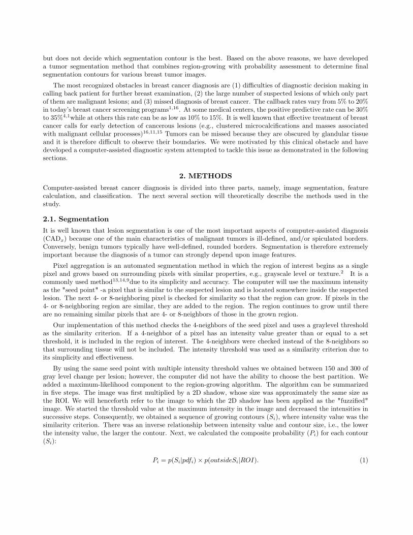
Pi = p(Si|pdfi)× p(outsideSi|ROI). (1)

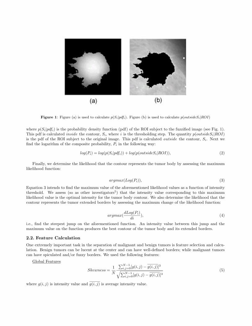
Figure 1: Figure (a) is used to calculate p(Si|pdfi). Figure (b) is used to calculate p(outsideSi|ROI)

where p(Si|pdfi) is the probability density function (pdf) of the ROI subject to the fuzzified image (see Fig. 1).This pdf is calculated inside the contour, Si, where i is the thresholding step. The quantity p(outsideSi|ROI)is the pdf of the ROI subject to the original image. This pdf is calculated outside the contour, Si. Next wefind the logarithm of the composite probability, Pi in the following way:

log(Pi) = log(p(Si|pdfi)) + log(p(outsideSi|ROI)), (2)

Finally, we determine the likelihood that the contour represents the tumor body by assessing the maximumlikelihood function:

argmax(Log(Pi)), (3)

Equation 3 intends to find the maximum value of the aforementioned likelihood values as a function of intensitythreshold. We assess (so as other investigators5) that the intensity value corresponding to this maximumlikelihood value is the optimal intensity for the tumor body contour. We also determine the likelihood that thecontour represents the tumor extended borders by assessing the maximum change of the likelihood function:

argmax(dLog(Pi)

di), (4)

i.e., find the steepest jump on the aforementioned function. An intensity value between this jump and themaximum value on the function produces the best contour of the tumor body and its extended borders.

2.2. Feature Calculation

One extremely important task in the separation of malignant and benign tumors is feature selection and calcu-lation. Benign tumors can be lucent at the center and can have well-defined borders; while malignant tumorscan have spiculated and/or fuzzy borders. We used the following features:

Global Features

Skewness =1

N

∑N−1i,j=0[g(i, j)− g(i, j)]3√∑N−1i,j=0[g(i, j)− g(i, j)]3

(5)

where g(i, j) is intensity value and g(i, j) is average intensity value.

Kurtosis =1

N

∑N−1i,j=0[g(i, j)− g(i, j)]4√∑N−1i,j=0[g(i, j)− g(i, j)]4

(6)

Circularity =A1

A, (7)

where A is the area of the actual ROI; A1 is the area of the overlapped region of A and the effective circle Ac,which is defined as the circle whose area is equal to A and is centered at the corresponding centroid of A.

Compactness =p2

a, (8)

where, p=tumor perimeter and a=tumor area

perimeter = tumor perimeter. (9)

Local FeaturesThese intensity features were calculated on the 10o ROI as it was divided into 10o sectors in the polar coordinatesystem, therefore each tumor contained 36 sectors.

g(i, j) =1

N

N−1∑i,j=0

g(i, j), (10)

where Mean = g(i, j), N is the total pixel number inside the ROI

Contrast =Pf − Pb

Pf, (11)

where Pf is the average gray-level inside the ROI’s and Pb is the average gray-level surrounding the ROI.

σ2f =

1

N

N∑i=1

(g(i, j)− g(i, j))2, (12)

where σ2f = standard deviation.

Area = tumor area (13)

σn =1

Nb

Nb∑i=1

(ri − r)2, (14)

where σn = Deviation of the Normalized Radial Length, Nb is the total number of pixels located on the boundaryof the ROI, ri is the value of the normalized radial length from the boundary coordinate (xi, yi) to the centroidof the ROI; r is the mean of ri.

Roughness = ([1

Nb

Nb∑i=1

(ri − r)4]14 − [

1

Nb

Nb∑i=1

(ri − r)2]12 ])/r. (15)

radial length = length of radius, (16)

where length of radius is the distance from the center of the tumor to its edge.

Given a second-order joint probability matrix Pd,θ(i, j), where Pd,θ(i, j) is the joint gray level distributionof a pixel pair (i,j) with the distance d and in the direction θ, six texture features are defined as follows:

Ed,θ(i, j) =L∑

i=1

L∑j=1

Pd,θ(i, j)2, (17)

where Ed,θ(i, j) = energy.

Id,θ(i, j) =L∑

i=1

L∑j=1

(i− j)2Pd,θ(i, j), (18)

where Id,θ(i, j) = inertia.

E =L∑

i=1

L∑j=1

Pd,θ(i, j)log2Pd,θ(i, j), (19)

where E = entropy.

IDMd,θ =L∑

i=1

L∑j=1

1

1 + (i− j)2Pd,θ(i, j), (20)

where, IDMd,θ = Inverse Difference Moment.

DEd,θ = −n−1∑k=0

Px−y(k)log2Px−y(k), Px−y(k) =n−1∑i=0

n−1∑j=0

Pd,θ(i, j), (21)

for |i− j| = k, k = 0, 1, ..., n− 1 where, DEd,θ = Difference Entropy.

2.3. Classifiers

We used a conventional backpropagation neural network for two of the three studies described in this paper.It is comprised of an input layer, one hidden layer, and one output. We used the multiple circular path neuralnetwork8 for the third study described in this paper. It is comprised of 3 input layers, one hidden layer andone output. The first input layer is fully connected, i.e., all inputs connect to all hidden nodes. The secondinput layer is called a self correlation path, i.e., each node on the layer connects to a single set of the 18 imagefeatures for the fan-in and fully connects to the hidden nodes for fan-out. The third input layer is called aneighborhood correlation path, i.e., each node on the layer connects to the input nodes of adjacent sectors forthe fan-in and fully connects to the hidden nodes for fan-out. Our study used 18 hidden layer nodes. A moredetailed explanation of the MCPCNN can be found the work done by Lo et. al.8.

3. EXPERIMENT

The image samples were chosen from several databases compiled by the ISIS Center of the Georgetown University(GU) Radiology Department and the University of Florida’s Digital Database for Screening Mammography(DDSM).3 They are a mixture of "obvious" cases and "not obvious" cases. The "obvious" cases contain tumorsthat are easily identifiable as malignant or benign while the "not obvious" cases are those that radiologists finddifficult to observe and/or classify. Forty malignant and forty benign tumors were tested during this experiment.The GU films were digitized at a resolution of 100µm using a Lumiscan digitizer. The DDSM films were digitizedat 43 and 50 µm’s using both the Lumiscan and Howtek digitizers. We compensated for this difference inresolution by reducing the DDSM images to half their normal sizes. The images were of varying contrasts andthe tumors were of varying sizes. There were 28 malignant cases and 23 benign cases.

Experiment Features Neural Network

1 Image Features Conventional NN

2 Image Features MCPCNN

3 ML-curve as features Conventional NN

Table 1: This table summarizes the studies presented in this paper.

The experiment was subdivided into three studies as shown in table 1 below.

Experiments 1 and 2 used 6 global and 12x36 sector features to yield a total of 438 image features per tumor.There were 18 hidden nodes and 1 output for both the BP and MCPCNN classifiers. The training and testingmethod used was the jackknife method. Experiment 3 used 19 likelihood feature values per tumor. There were15 hidden nodes and 1 output for the BP classifier. The training and testing method used was the jackknifemethod. The results were analyzed using the LABROC4 program.10

4. RESULTS

Here are two examples of segmentation results for both malignant (see Fig. 2) and benign (see Fig. 4) cases.Each example gives the segmentation result produced by the maximum likelihood value on the curves describedin section 2.1.

The following is a table, which gives the Az values produced by the neural network.

Experiment Features Neural Network Az

1 Image Features Conventional NN 0.66

2 Image Features MCPCNN 0.71

3 ML-curve as features Conventional NN 0.84

Table 2: Results from Experiments 1-3.

5. CONCLUSION AND DISCUSSION

In analyzing the segmentation results we drew several conclusions. We discovered that there was a markeddifference between the likelihood functions in malignant cases and the likelihood functions in benign cases.The likelihood function in the benign case often experiences a sharp drop, while the likelihood function in themalignant case is often smoother. In the image, a sharp drop value in the likelihood function represents anabrupt change in the area as well as likelihood value. We observed thatin benign cases, the likelihood functionsharp changes are much more evident because benign tumors usually have well-defined borders. Conversely, inmany malignant cases, the likelihood functions are smoother because many of their the borders are ill-defined. Inanalyzing the likelihood functions for malignant cases we recognized that those curves with very sharp changeswere produced from tumors with well-defined borders and vice versa; i.e., there were malignant tumors thatcould be mistaken as benign and vice versa.

The maximum likelihood curves used as inputs to the BP neural network produced the best performanceoverall. The image features used as inputs to the MCPCNN produced the second best performance. The imagefeatures used as inputs to the BP produced the worst performance. Since we received the best results by usingthe likelihood functions as features, we expect that the MCPCNN may improve the overall results by givingthe likelihood functions in every sector.

Figure 2. The segmentation results for a malignant tumor. Part (a) shows the segmentation result produced by themaximum likelihood change intensity choice, part (b) shows the original image, and part (c) shows the segmentationresult produced by the maximum likelihood intensity choice.

..

Figure 3. A likelihood function with respect to threshold values for all segmentation steps (malignant case) shown inFig. 2.

ACKNOWLEDGMENTS

This work has been supported by the following grants: DAMD17-00-1-0291, DAAG55-98-1-0187, and DAMD17-00-1-0267.

Figure 4. The segmentation results for a benign tumor. Part (a) shows the segmentation result produced by themaximum likelihood change intensity choice, part (b) shows the original image, and part (c) shows the segmentationresult produced by the maximum likelihood intensity choice.

..

Figure 5. A likelihood function with respect to threshold values for all segmentation steps (benign case) shown in Fig. 4.

REFERENCES

1. Frankel SD, Sickel EA, Curpen BN, Sollito RA, Ominsky SH, Galvin HB, Initial versus subsequentscreening mammography: Comparison of findings and their prognostics significance. AJR, 1995, vol.164, pp. 1107-1109.

2. Gonzalez RC, Woods RE. Digital Image Processing Reading, MA: Addison Wesley, 1992.

3. Heath M, Bowyer KW, Kopans D et al, Current status of the Digital Database for Screening Mam-mography, Digital Mammography, Kluwer Academic Publishers, 1998, pp. 457-460.

4. Kopans DB. The positive predictive value of mammography, AJR, 1991, vol. 158, pp. 521-526.

5. Kupinski MA, Giger ML, Automated Seeded Lesion Segmentation on Digital Mammograms, IEEETransactions on Medical Imaging, 1998, vol. 17, no. 4, pp. 510-517.

6. Li L, Zheng Y, Zhang L, Clark R, False-positive reduction in CAD mass detection using a competitiveclassification strategy, Medical Physics, 2001, Vol. 28, no. 2, pp. 250-258.

7. Li H, Wang Y, Liu KJR, Lo S-C, Freedman MT, Computerized Radiographic Mass Detection - Part I:Lesion Site Selection by Morphological Enhancement and Contextual Segmentation, IEEE Transac-tions on Medical Imaging, 2001, vol. 20, no. 4, pp. 289-301.

8. Lo SC, Li H, Wang J, Kinnard L, Freedman MT,A Multiple Circular Path Convolution Neural NetworkSystem for Detection of Mammographic Masses, IEEE Transactions on Medical Imaging, 2002, vol. 21,No. 2, (Accepted for publication).

9. Mendez AJ, Tahoces PG, Lado MJ, Souto M., Vidal JJ,Computer-aided diagnosis: Automatic detectionof malignant masses in digitzed mammograms, Medical Physics, 1998, vol. 25, no. 6, pp. 957-964.

10. Metz C, LABROC Program, ftp://radiology.uchicago.edu/roc.

11. Nystrom L, Rutqvist LE, Wall S, Lindgren A, Lindqvist M, Ryden S, et. al., Breast cancer screeningwith mammography: Overview of Swedish randomized trials, Lancet, 1993, vol. 341, pp. 973-978.

12. Petrick N, Chan H-P, Sahiner B, Wei D, An Adaptive Density-Weighted Contrast Enhancement Filterfor Mammographic Breast Mass Detection, IEEE Transactions on Medical Imaging, 1996, vol. 15, no.1, pp. 59-67.

13. Pohlman S, Powell KA, Obuchowski NA, Chilcote WA, Grundfest-Broniatowski S, Quantitative classifi-cation of breast tumors in digitized mammograms, Medical Physics, 1996, vol. 23, no. 8, pp. 1336-1345.

14. Sahiner B, Chan HP, Wei D, Petrick N, Helvie MA, Adler DD, Goodsit MM, Image feature selection bya genetic algorithm: Application to classification of mass and normal breast tissue, Medical Physics,1996, vol. 23, no. 10, pp. 1671-1684.

15. Shapiro S, Screening: Assessment of current studies, Cancer, 1994, vol. 74, pp.231-238.

16. Tabar L, Fagerberg G, Duffy S, Day NE, Gad A, Grontoft O. Update of the Swedish two-country programof mammographic screening for breast cancer, Radiology Clinics of North America: Breast Imaging -Current Status and Future Directions, 1992, vol. 30, pp. 187-210.

150 IEEE TRANSACTIONS ON MEDICAL IMAGING, VOL. 21, NO. 2, FEBRUARY 2002

A Multiple Circular Path ConvolutionNeural Network System for Detection

of Mammographic MassesShih-Chung B. Lo*, Member, IEEE, Huai Li, Member, IEEE, Yue Wang, Member, IEEE, Lisa Kinnard, and

Matthew T. Freedman

Abstract—A multiple circular path convolution neural network(MCPCNN) architecture specifically designed for the analysis oftumor and tumor-like structures has been constructed. We firstdivided each suspected tumor area into sectors and computed thedefined mass features for each sector independently. These sectorfeatures were used on the input layer and were coordinated by con-volution kernels of different sizes that propagated signals to thesecond layer in the neural network system. The convolution ker-nels were trained, as required, by presenting the training cases tothe neural network.

In this study, randomly selected mammograms were processedby a dual morphological enhancement technique. Radiodenseareas were isolated and were delineated using a region growing al-gorithm. The boundary of each region of interest was then dividedinto 36 sectors using 36 equi-angular dividers radiated from thecenter of the region. A total of 144 Breast Imaging—Reportingand Data System-based features (i.e., four features per sector for36 sectors) were computed as input values for the evaluation of thisnewly invented neural network system. The overall performancewas 0.78–0.80 for the areas ( ) under the receiver operatingcharacteristic curves using the conventional feed-forward neuralnetwork in the detection of mammographic masses. The perfor-mance was markedly improved with values ranging from 0.84to 0.89 using the MCPCNN. This paper does not intend to claimthe best mass detection system. Instead it reports a potentiallybetter neural network structure for analyzing a set of the massfeatures defined by an investigator.

Manuscript received February 22, 2000; revised January 11, 2002. This workwas supported by the US Army under Grant DAMD17-96-1-6254 througha subcontract from University of Michigan, Ann Arbor, and under GrantDAMD17-01-1-0267 through a subcontract from Howard University. The workof Y. Wang was supported by the US Army under Grant DAMD17-98-1-8045.The work of L. Kinnard was supported by the US Army under Grant DAMD17-00-1-0291. The content of this paper does not necessarily reflect theposition or policy of the government. The Associate Editor responsible forcoordinating the review of this paper and recommending its publication was N.Karssemeijer.Asterisk indicates corresponding author.

*S.-C. B. Lo is with the Center for Imaging Science and InformationSystem, Radiology Department, Georgetown University Medical Center, 2115Wisconsin Avenue, Suite 603, N.W., Washington, DC 20007 USA (e-mail:lo@isis.imac.georgetown.edu).

H. Li was with the ISIS Center, Radiology Department, Georgetown Univer-sity Medical Center, Washington, DC 20007 USA. He is now with the Centerfor Information Technology, Division of Computational Bioscience, NationalInstitutes of Health, Bethesda, MD 20892 USA.

Y. Wang is with the Department of Electrical Engineering and Computer Sci-ences, The Catholic University of America, Washington, DC 20064 USA.

L. Kinnard is with the Center for Imaging Science and Information System,Radiology Department, Georgetown University Medical Center, Washington,DC 20007 USA, and also with the Department of Electrical Engineering,Howard University, Washington, DC 20059 USA.

M. T. Freedman is with the Center for Imaging Science and InformationSystem, Radiology Department, Georgetown University Medical Center, Wash-ington, DC 20007 USA.

Publisher Item Identifier S 0278-0062(02)02935-X.

Index Terms—BI—RAD, computer-aided diagnosis, convolu-tion neural network, mammography masses, neural network,sector features.

I. INTRODUCTION

I T IS KNOWN that effective treatment of breast cancer callsfor early detection of cancerous lesions (e.g., clustered mi-

crocalcifications and masses associated with malignant cellularprocesses) [1]–[3]. Breast masses appear as areas of increaseddensity on mammograms. It is particularly difficult for radi-ologists to detect and analyze a suspected area where a massis overlapped with dense breast tissue. These masses are morereadily seen as time progresses, but the further the tumor hasprogressed, the lower the possibility of a successful treatment.Therefore, increasing the chances of early breast cancer detec-tion in improving today’s clinical system is of vital importancein breast cancer diagnosis.

Several research groups have developed computer algorithmsfor automated detection of mammographic masses [4]–[8].Some of these methods involved in classification of masses andnormal dense breast tissues [7], [8]. Investigators also attemptedto classify the malignant or benign nature of the detected tu-mors [9]–[11]. It is conceivable that correct segmentation of themasses [12] plays an important processing step prior to furthermass analysis. In short, the results of these detection programsindicate that a high true-positive (TP) rate can be obtainedat the expense of two or three false-positive (FP) detectionsper mammogram. Mammographically, a multiplicity (morethan two) of similar benign-appearing breast lesions arguesstrongly for benignity [13]–[16] and, indeed, the more massesthat are identified, the less chance that they represent cancer[17]. If the computer indicates multiple suspicious locationson a mammogram, the radiologist has to seek out one massthat possesses mammographic features, which are differentfrom the others. The significant lesion may be missed due tothe multiplicity of possible lesions. We, therefore, believe thata more useful and fundamental approach to computer-aideddiagnosis (CAD) of masses is to devise computer programs toanalyze features of a suspected area [18], [19] and to providefeature measures and estimates of the likelihood of malignancyby making comparisons within a digital mammographicdatabase. The computer, therefore, serves as a second opinionand also provides a reproducible and an objective evaluationof the mass. With this aid, the radiologist may also increasehis/her sensitivity by lowering the threshold of suspicion, whilemaintaining the overall specificity and reading efficiency.

0278-0062/02$17.00 © 2002 IEEE

LO et al.: A MCPCNN SYSTEM FOR DETECTION OF MAMMOGRAPHIC MASSES 151

II. CLINICAL BACKGROUND OF BREAST LESIONS AND

TECHNICAL APPROACH INMASS DETECTION

A. Description of Clinical Background

Most commonly, breast cancer presents itself as a mass. Thesame lesion shows a somewhat different picture from one pro-jection to the other. Difficulties in masses also vary with theunderlying breast parenchyma. In the fatty breast, masses aregenerally easy to detect. In the dense breast, mass detectionis more difficult and auxiliary signs aid this detection. Whenthe breast contains one mass, the decision process is based onits size, shape, and margins. When there are several masses,one looks at each, trying to determine whether any has fea-tures to suggest cancer. Furthermore, one looks to see if anymass is different in appearance from the others. Multiple small,well-defined, similar masses that present themselves bilaterallyare all likely to be benign. Large, poorly defined, spiculatedand unusually radiodense masses are extremely likely to be ma-lignant. In this study, we used several computational features(see Section III-B) highly associated with four major featuresof breast masses routinely used in clinical reading:

Density: Malignant lesions tend to have greater radio-graphic density due to high attenuation and lesscompressibility of cancer than normal tissue.Radiolucent lesions are typically benign and thediagnosis can be made from the mammogram.

Size: If the lesion has morphological features sug-gesting malignancy, it should be consideredsuspicious regardless of the size. Isolatedmasses with noncystic densities greater than8 mm in diameter can be malignant. In general,the larger a lesion, the more suspicious it is.

Shape: The more irregular the shape of a lesion, themore likely the possibility of malignancy. Le-sions tend to be round, ovoid and/or lobulated.Small and frequent lobulations are suspicious.Lesions in the lateral aspect of the breast near theedge of the parenchyma with a reniform shapeand a hilar indentation or notch usually repre-sent a benign intramammary lymph node. Breastcarcinoma hidden in the dense tissues can causeparenchymal retraction, which possess differentshapes.

Margins: The margins of the lesion should be carefullyevaluated for areas of spiculation, stellate pat-terns or ill-defined regions. Most breast cancershave ill-defined margins secondary to tumor in-filtration and associated fibrosis. The appearanceof spiculations and a more diffuse stellate pat-tern are almost pathognomonic for cancer. Le-sions with sharply defined margins have a highlikelihood of being benign; however, up to 7% ofmalignant lesions can be well circumscribed.

These are known clinical features and have been adapted in“Breast Imaging—Reporting and Data System” (BI—RAD)[20] of the American College of Radiology. Fig. 1(a) and (b)shows two breast images containing masses. In Fig. 1(a), amalignant mass is superimposed on the dense glandular tissue.

Fig. 1. (a) Dense breast containing a malignant mass. (b) Fatty and glandularbreast containing a malignant mass.

However, its spiculated nature makes it easily identifiable.In Fig. 1(b), another malignant mass is located on the fattybackground but is associated with a large body of glandulartissue. This mass is not easily detectable by the computerbecause its density is lower than the neighboring glandulartissue. Furthermore, one end of the mass is fully connectedwith this tissue.

B. Technical Approach for Detection of MammographicMasses

In this study, our goal was to detect clinically suspicious le-sions. The differentiation of benign and malignant status of themammographic masses can be extended from this study modeland will be reported in our future work. The study was con-ducted with the following steps: 1) use background correctionmethod and morphological operations to extract radio-opaqueareas; 2) delineate the boundary of the areas; 3) compute the fea-tures and texture of the masses with emphasis on the boundary;and 4) design training strategy using neural networks as classi-fiers for the recognition of mass features. The overall detectionscheme of the study framework is shown in Fig. 2.

III. D EVELOPMENT OFTECHNICAL METHODS

A. Preprocessing and Extraction of Suspicious Masses

In automatic mass detection, accurate selection of suspectedmasses is considered a critical first step due to the variabilityof normal breast tissue and the lower contrast and ill-definedmargins of masses. In our previous study [18], we aimed to im-prove the task of lesion site selection using model-based imageprocessing techniques for unsupervised lesion site selection. Wefocused on two essential issues in the stochastic model-basedimage segmentation: enhancement and model selection. Basedon the differential geometric characteristics of masses against

152 IEEE TRANSACTIONS ON MEDICAL IMAGING, VOL. 21, NO. 2, FEBRUARY 2002

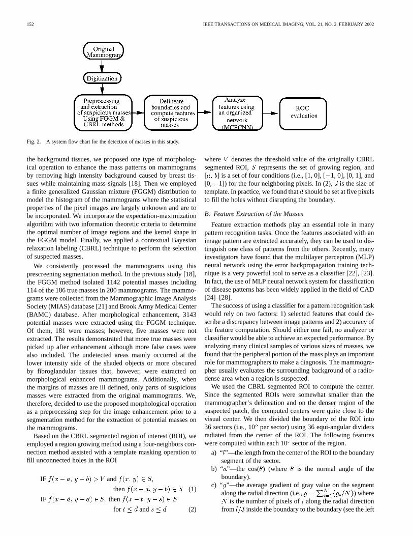
Fig. 2. A system flow chart for the detection of masses in this study.

the background tissues, we proposed one type of morpholog-ical operation to enhance the mass patterns on mammogramsby removing high intensity background caused by breast tis-sues while maintaining mass-signals [18]. Then we employeda finite generalized Gaussian mixture (FGGM) distribution tomodel the histogram of the mammograms where the statisticalproperties of the pixel images are largely unknown and are tobe incorporated. We incorporate the expectation-maximizationalgorithm with two information theoretic criteria to determinethe optimal number of image regions and the kernel shape inthe FGGM model. Finally, we applied a contextual Bayesianrelaxation labeling (CBRL) technique to perform the selectionof suspected masses.

We consistently processed the mammograms using thisprescreening segmentation method. In the previous study [18],the FGGM method isolated 1142 potential masses including114 of the 186 true masses in 200 mammograms. The mammo-grams were collected from the Mammographic Image AnalysisSociety (MIAS) database [21] and Brook Army Medical Center(BAMC) database. After morphological enhancement, 3143potential masses were extracted using the FGGM technique.Of them, 181 were masses; however, five masses were notextracted. The results demonstrated that more true masses werepicked up after enhancement although more false cases werealso included. The undetected areas mainly occurred at thelower intensity side of the shaded objects or more obscuredby fibroglandular tissues that, however, were extracted onmorphological enhanced mammograms. Additionally, whenthe margins of masses are ill defined, only parts of suspiciousmasses were extracted from the original mammograms. We,therefore, decided to use the proposed morphological operationas a preprocessing step for the image enhancement prior to asegmentation method for the extraction of potential masses onthe mammograms.

Based on the CBRL segmented region of interest (ROI), weemployed a region growing method using a four-neighbors con-nection method assisted with a template masking operation tofill unconnected holes in the ROI

IF and

then (1)

IF then

for and (2)

where denotes the threshold value of the originally CBRLsegmented ROI, represents the set of growing region, and[ ] is a set of four conditions (i.e., [1, 0], [1, 0], [0, 1], and[0, 1]) for the four neighboring pixels. In (2), is the size oftemplate. In practice, we found thatshould be set at five pixelsto fill the holes without disrupting the boundary.

B. Feature Extraction of the Masses

Feature extraction methods play an essential role in manypattern recognition tasks. Once the features associated with animage pattern are extracted accurately, they can be used to dis-tinguish one class of patterns from the others. Recently, manyinvestigators have found that the multilayer perceptron (MLP)neural network using the error backpropagation training tech-nique is a very powerful tool to serve as a classifier [22], [23].In fact, the use of MLP neural network system for classificationof disease patterns has been widely applied in the field of CAD[24]–[28].

The success of using a classifier for a pattern recognition taskwould rely on two factors: 1) selected features that could de-scribe a discrepancy between image patterns and 2) accuracy ofthe feature computation. Should either one fail, no analyzer orclassifier would be able to achieve an expected performance. Byanalyzing many clinical samples of various sizes of masses, wefound that the peripheral portion of the mass plays an importantrole for mammographers to make a diagnosis. The mammogra-pher usually evaluates the surrounding background of a radio-dense area when a region is suspected.

We used the CBRL segmented ROI to compute the center.Since the segmented ROIs were somewhat smaller than themammographer’s delineation and on the denser region of thesuspected patch, the computed centers were quite close to thevisual center. We then divided the boundary of the ROI into36 sectors (i.e., 10per sector) using 36 equi-angular dividersradiated from the center of the ROI. The following featureswere computed within each 10sector of the region.

a) “ ”—the length from the center of the ROI to the boundarysegment of the sector.

b) “ ”—the cos( ) (where is the normal angle of theboundary).

c) “ ”—the average gradient of gray value on the segmentalong the radial direction (i.e., ) where

is the number of pixels of along the radial directionfrom inside the boundary to the boundary (see the left

LO et al.: A MCPCNN SYSTEM FOR DETECTION OF MAMMOGRAPHIC MASSES 153

Fig. 3. A suspicious mass is delineated and shown as the shaded region.Contrast is computed by subtracting the average background pixel value(i.e., b , o = 1; 2; . . .P ) from the average foreground value (i.e.,h ,i = 1; 2; . . .P ).

line segment, Fig. 3). Technically speaking, this setof gradient values may also serve as a fuzzy system onthe input layer in the neural network (to be described inSection III-C).

d) “ ”—the gray value difference (i.e., contrast)along the radial direction. Specifically,

where (or )represents a pixel value along the radial direction. Theposition inside the boundary is the center of pixels

( ) and position outside theboundary is the center of pixels ( ),and is the number of pixels equivalent to a segment of

and was used for averaging (see Fig. 3).Hence, a total of 144 computed features (four features/sector

for 36 sectors) were used as input values for the classificationof the ROI. The relationship between the computed features andBI—RADS descriptors are discussed below.

i) ROI Size—The size of ROI is provided by the 36 “”values.

ii) ROI Shape (round, oval, lobulated, or irregular)—The 36“ ” and 36 “ ” values can describe the shape of the ROI.

iii) ROI Margin (circumscribed, microlobulated, obscured,ill- defined, or spiculate)—The 36 “” and 36 “ ” valuescan describe the ROI margin.

iv) ROI Density (fat-containing, low density, isodense, orhighly dense)—The 36 “” and 36 “ ” values can be usedto describe the density distribution of the ROI.

In short, the selected features are greatly associated with themain mass descriptors indicated in the BI—RADS. The reasonfor using 36 values for each nominated feature is four-fold:1) mass boundary varies, it is difficult to describe an image pat-tern using a single value; 2) due to the general shape of themasses, the features of masses can be easily analyzed by thepolar coordinate system; 3) in case some features are inaccu-rately computed in several directions due to the structure noises,such as the breast slender lines, there may still exist a suffi-cient number of correct features; and 4) generally more accu-rate results can be produced by using subdivided parametersrather than using global parameters in a pattern recognition taskwhen the parameters are barely discernable and sample sizes aresufficiently large. Other computational features (e.g., difference

entropy [19] and other higher order features) are eligible but re-quire further investigation.

C. The Neural Network Structure Specifically Designed for theExtracted Boundary Features

1) Multiple Paths With Circular Networking to Instruct theNeural Network in Analyzing Sector Features:This paperfocuses on neural network design and arrangement of featuresfor effective pattern recognition of ROIs. We designed severalneural network connections between the input and the firsthidden layers as shown in Fig. 4. In this neural network system,the first layer also functions as a correlation layer that trans-forms and encodes the signals from input nodes into correlationfeatures for further neural network process. Fig. 4(a)–(c) illus-trates the full connection (FC), a self correlation (SC) network,and a neighborhood correlation (NC) network, respectively.Network connections with multiple sectors (i.e., 20, 30 , 40 ,and 50 of the NC) are grouped separately as independent NCpaths. In the following study, we used four SC paths for a singlesector and thirteen NC paths for four types of multisectors.The method of using the multiple correlation connectionswas motivated by our research experience in two-dimensional(2-D) convolution neural network (CNN) [(2-D CNN)] wherewe found that more than ten multiple convolution kernels inthe CNN were necessary in the detection of lung nodules andmicrocalcifications [25].

Compared with 2-D CNN systems, the computation requiredin the one-dimensional (1-D) CNN (e.g., 144 input features)is relatively small. The combination of the networking pathsdescribed earlier for multiple circular path convolution neuralnetwork (MCPCNN) was implemented using C programminglanguage. The internal computation algorithm used in theMCPCNN shares the same convolution process as that in the2-D CNN [25]. Rotation invariance and flip invariance fortraining the 1-D convolution kernels in the MCPCNN wereemployed.

The fully connected neural network is a conventional feed-forward MLP neural network. The signals of the fully connectedneural network join the other network processes (i.e., SC pathsand NC paths) at the single node of the output layer. The signalreceived at the output node is scaled between zero and one.During the training, zero and one were assigned at the outputnode to perform backpropagation computation for a nonmassand a mass, respectively. The backpropagation is computed insuch a way that the computed incremental errors [see equations(9) and (10)] are retraced into every independent network path.Excluding the output layer, the SC and NC signals are indepen-dently arranged and are processed through the 1-D convolutionprocess in the forward propagation. The learning algorithms forall three types of circular network paths are based on the back-propagation training method.

Let ( , ) represents an input signal at the nodeandsector . The signal processed through an NC path and to bereceived at each node,, on the first hidden layer is

(3)

154 IEEE TRANSACTIONS ON MEDICAL IMAGING, VOL. 21, NO. 2, FEBRUARY 2002

Fig. 4. Three types of network paths connecting the input and the hidden layers in the MCPCNN. (a) FC path. (b) SC path. Eeach node on the layer connectsto a single set of the features (l, a, g, c) for the fan-in and fully connects to the hidden nodes for fan-out. (c) A NC path. Each node on the layer connects to theinput nodes of adjacent sectors for the fan-in and fully connects to the hidden nodes for fan-out. The fan-in nets emphasizing SC in (b) and NC in (c) representconvolution weights (i.e., the same type of sectors possess the same set of weighting factors).

where represents the bias term andis an array associated the 2-D nets that fan-in to a given receivingnode, . Each element of is the weight factorconnected to node from node sector through a NC path,, and covers a range of neighborhood sectors corresponding

to each type of NC path. Note that multiplications between theinput nodes and connecting weights are computed first followedby taking the sum of the products for those nodes and sectors in-volved. The operation is repeated by shifting the weights fromone set of sectors to the next. The procedure involving arraymultiplication passing through every sector is referred as the1-D convolution operation that takes place in the sector dimen-sion. The signal processed through an SC path and to be receivedat a node, , on the first hidden layer is a special case of an NCpath when only covers one sector

(4)where is the weight factor connected tofromnode through a SC path,, regardless of the sectors. A totalof 18 paths (1 FC, 4 SC paths, and 13 NC paths for four typesof multisectors) were used in our experiment described later.Nevertheless, the signals processed through a path and to bereceived at each node,, on the first hidden layer is

(5)

where is one of the network paths and is a sigmoid func-tion given by

(6)

The sigmoid function would produce modulated values rangingfrom zero to one. The signals on other hidden layers in each pathare processed the same as a conventional fully connected neuralnetwork. Other than the first hidden layer, the receiving signalsat a hidden layer,, collected from the previous hidden layer,to one, are merged from the nodes in the last layer and are givenby

(7)

where and denote the nodes at layers and ,respectively.

Let the th change of the weight be and theth change of the bias be . The error function is defined

as

(8)

where and denote the target output value and the actualoutput value, respectively when the input values , are

LO et al.: A MCPCNN SYSTEM FOR DETECTION OF MAMMOGRAPHIC MASSES 155

Fig. 5. A schematic diagram, showing the MCPCNN and sector features of masses, that was used in the following study.

entered in the network. In this model, the error backpropagationalgorithm, which updates the kernel weights, is given below

(9)

(10)

(11)

In the case of the last layer

(12)

where , , , and denote the derivative of ,the learning rate, the weighting factor contributed by themomentum term, and the desired output image, respectively.Furthermore, or and when .

During the training, we added an isotropic constraint to theweights of the 1-D convolution kernels so that

(13)

where is not the fully connected path. These additional con-straints are used to induce the kernels functioning as correlationprocessing filters and could facilitate the algorithm in searchingfor an appropriate filter.

2) Resampling the Training Set Through Utilization of Rota-tion and Flip Invariance of the Features:In this neural networkmodel, there are no starting and ending sectors. The forward andbackpropagation computation can start from any sector. Consid-ering a flipped patch, the characteristics of mass feature shouldremain the same. To take advantage of this flip invariance, thesame numerical target value can be assigned at the output node

for the flipped image patch in order to double the amount ofcases during training.

Since we designed a 10increment for each rotation, everySC or NC path would process through 36 times using the de-fined features for each image patch. To simplify this networkcomputation, we shifted one small sector (four nodes) on theinput layer at a time to conduct the circular convolution processwith the SC and NC kernels in the following experiments. Byreversing the sequence of the sector, one can train the flippedversion of the suspicious masses. Hence, using the propertiesof the rotation invariance and flip invariance for the neural net-work training literally increases the number of the training setby a factor of 72.

In summary, we have developed a complete detection pro-cedure for the automatic recognition of mammographic massesincluding background adjustment, contrast enhancement, ROIsegmentation, feature extraction, and MCPCNN system with atraining method. Fig. 5 shows a flow diagram for the essentialsections of the computational procedures.

IV. EXPERIMENTS AND RESULTS

As described in Section III-A, the 200 mammograms were se-lected from the MIAS database and the BAMC database for thestudy. Of the 200 mammograms, 50 mammograms are normal,and each of the 150 abnormal mammograms contains at leastone mass case of varying size, subtlety, and location. Both thecranio-caudal (CC) and medio-lateral oblique (MLO) projec-tion views were used. The films were digitized with a com-puter format of 2048 2500 12 bits (for an areawhere each image pixel represents 100m square). Ninety-onemammograms, either a CC or an MLO view film, were selectedfrom 91 patient film jackets. No two mammograms were se-lected from the same patient. All the digitized mammogramswere miniaturized to 512 625 12 bits using pixel av-eraging before the method was applied. According to radiolo-gists, the size of small masses is 3–15 mm in effective diameter.A 3-mm object in an original mammogram occupies 30 pixelsin a digitized image with a 100–m resolution. After reducingthe image size by four times, the object will occupy the rangeof about 7–8 pixels. The object with the size of seven pixels

156 IEEE TRANSACTIONS ON MEDICAL IMAGING, VOL. 21, NO. 2, FEBRUARY 2002

is expected to be detectable by any computer algorithm. Afterpreprocessing and an object screening based on the circularitytest and the size test (between 3 and 30 mm), a total of 125 sus-picious areas were selected from the testing mammograms (91cases) for this study. Specifically, the screening procedure of re-ducing FPs involves two steps: 1) image patches with circularityless than 0.25 or diameter greater than 30 mm were eliminatedand 2) ) using probability modular neural network to rule outthe majority of FPs. Of the 125 suspicious areas, 75 ROIs con-tained masses based on corresponding biopsy reports with oneexperienced radiologist reading. Of 75 masses, 39 were malig-nant and 36 were benign. This set of ROIs was used in [19] anddiscussed in [19, Fig. 6 and Table II].

A. Experiment 1

Of the 125 suspicious areas, we randomly selected 54 com-puter-segmented ROIs where 30 patches were matched with theradiologist’s mass identification and 24 were not. This databasewas used to train two neural network systems: 1) a conven-tional three-layer neural network and 2) the proposed MCPCNNtraining method using the same neural network learning algo-rithm. The structure of the MCPCNN was described earlier. Inthe study, we used one fully connected path, four SC paths, fourNC paths covering two sectors, four NC paths covering threesectors, three NC paths covering four sectors, and two NC pathscovering five sectors in the first step network connection for theMCPCNN. All paths in the neural network have their hiddenlayers. Only one hidden layer per path was used. Both neuralnetwork systems were trained by the error backpropagation al-gorithm by feeding the features from the input layer and regis-tering the corresponding target value at the output node. Com-pletion of the training was determined by the mean square error[i.e., , where is number of samples] whenit was approximately reduced to 310 . Once the training ofthe neural networks was completed, we then used the remaining71 computer segmented ROIs for the testing. Forty-five out of 71ROIs were masses and 26 ROIs were not. Neither the images northeir corresponding patients in the testing set could be found inthe training set. The neural network output values were fed intothe LABROC4 program [29] for the performance evaluation.The results indicated that the areas () under the receiver op-erating characteristic (ROC) curves were 0.78690.0536 and0.8443 0.0457 using the conventional neural network (MLP)and the MCPCNN, respectively. The ROC curves of these twoneural network systems are shown in Fig. 6(a). Thevaluewas 0.7869 0.0536 when using the MLP method with 125hidden nodes. The performance of the MLP remains about thesame at 0.7809 0.0551 of using the same neural networkparameters but with 30 hidden nodes.

We also invited another senior mammographer to conduct anobserver study using the ROC study protocol. The mammogra-pher was asked to rate each patch using a numerical scale rang-ingfrom zero to ten for its likelihood of being a breast mass.The image patches were displayed on a SUN monitor (Model:GDM-20D10). The image size shown on the monitor was re-duced to approximately as compared with the originalfilm size ( ). These 71 numbers were also fed into theLABROC4 program. The of the mammographer’s perfor-

(a)

(b)

Fig. 6. The ROC curves obtained from corresponding experiments. (a) Showsthat the performance of MCPCNN training method is superior to that of theconventional MLP method. The highest curve is the ROC performance of thesenior mammographer. (b) Shows that the ROC results were increased using theleave-one-case-out procedure in both neural network systems. The MCPCNNstill showed higher performance than conventional MLP method.

mance on this set of test cases was 0.9090.0340. The corre-sponding ROC curve is also shown in Fig. 6(a).

B. Experiment 2

We also conducted a leave-one-case-out experiment (i.e.,jackknife procedure) using the same database. In this ex-periment, we used those image patches extracted from 90

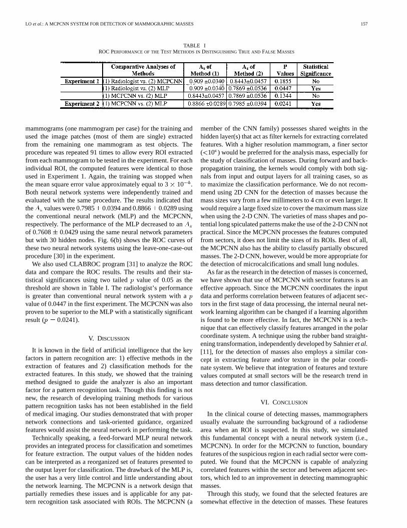
LO et al.: A MCPCNN SYSTEM FOR DETECTION OF MAMMOGRAPHIC MASSES 157

TABLE IROC PERFORMANCE OF THETEST METHODS IN DISTINGUISHING TRUE AND FALSE MASSES

mammograms (one mammogram per case) for the training andused the image patches (most of them are single) extractedfrom the remaining one mammogram as test objects. Theprocedure was repeated 91 times to allow every ROI extractedfrom each mammogram to be tested in the experiment. For eachindividual ROI, the computed features were identical to thoseused in Experiment 1. Again, the training was stopped whenthe mean square error value approximately equal to 310 .Both neural network systems were independently trained andevaluated with the same procedure. The results indicated thatthe values were 0.7985 0.0394 and 0.8866 0.0289 usingthe conventional neural network (MLP) and the MCPCNN,respectively. The performance of the MLP decreased to anof 0.7608 0.0429 using the same neural network parametersbut with 30 hidden nodes. Fig. 6(b) shows the ROC curves ofthese two neural network systems using the leave-one-case-outprocedure [30] in the experiment.

We also used CLABROC program [31] to analyze the ROCdata and compare the ROC results. The results and their sta-tistical significances using two tailed value of 0.05 as thethreshold are shown in Table I. The radiologist’s performanceis greater than conventional neural network system with avalue of 0.0447 in the first experiment. The MCPCNN was alsoproven to be superior to the MLP with a statistically significantresult ( 0.0241).

V. DISCUSSION

It is known in the field of artificial intelligence that the keyfactors in pattern recognition are: 1) effective methods in theextraction of features and 2) classification methods for theextracted features. In this study, we showed that the trainingmethod designed to guide the analyzer is also an importantfactor for a pattern recognition task. Though this finding is notnew, the research of developing training methods for variouspattern recognition tasks has not been established in the fieldof medical imaging. Our studies demonstrated that with propernetwork connections and task-oriented guidance, organizedfeatures would assist the neural network in performing the task.

Technically speaking, a feed-forward MLP neural networkprovides an integrated process for classification and sometimesfor feature extraction. The output values of the hidden nodescan be interpreted as a reorganized set of features presented tothe output layer for classification. The drawback of the MLP is,the user has a very little control and little understanding aboutthe network learning. The MCPCNN is a network design thatpartially remedies these issues and is applicable for any pat-tern recognition task associated with ROIs. The MCPCNN (a

member of the CNN family) possesses shared weights in thehidden layer(s) that act as filter kernels for extracting correlatedfeatures. With a higher resolution mammogram, a finer sector( 10 ) would be preferred for the analysis mass, especially forthe study of classification of masses. During forward and back-propagation training, the kernels would comply with both sig-nals from input and output layers for all training cases, so asto maximize the classification performance. We do not recom-mend using 2D CNN for the detection of masses because themass sizes vary from a few millimeters to 4 cm or even larger. Itwould require a large fixed size to cover the maximum mass sizewhen using the 2-D CNN. The varieties of mass shapes and po-tential long spiculated patterns make the use of the 2-D CNN notpractical. Since the MCPCNN processes the features computedfrom sectors, it does not limit the sizes of its ROIs. Best of all,the MCPCNN also has the ability to classify partially obscuredmasses. The 2-D CNN, however, would be more appropriate forthe detection of microcalcifications and small lung nodules.

As far as the research in the detection of masses is concerned,we have shown that use of MCPCNN with sector features is aneffective approach. Since the MCPCNN coordinates the inputdata and performs correlation between features of adjacent sec-tors in the first stage of data processing, the internal neural net-work learning algorithm can be changed if a learning algorithmis found to be more effective. In fact, the MCPCNN is a tech-nique that can effectively classify features arranged in the polarcoordinate system. A technique using the rubber band straight-ening transformation, independently developed by Sahnieret al.[11], for the detection of masses also employs a similar con-cept in extracting feature and/or texture in the polar coordi-nate system. We believe that integration of features and texturevalues computed at small sectors will be the research trend inmass detection and tumor classification.

VI. CONCLUSION

In the clinical course of detecting masses, mammographersusually evaluate the surrounding background of a radiodensearea when an ROI is suspected. In this study, we simulatedthis fundamental concept with a neural network system (i.e.,MCPCNN). In order for the MCPCNN to function, boundaryfeatures of the suspicious region in each radial sector were com-puted. We found that the MCPCNN is capable of analyzingcorrelated features within the sector and between adjacent sec-tors, which led to an improvement in detecting mammographicmasses.

Through this study, we found that the selected features aresomewhat effective in the detection of masses. These features

158 IEEE TRANSACTIONS ON MEDICAL IMAGING, VOL. 21, NO. 2, FEBRUARY 2002

were “computationally translated” from the qualitative descrip-tors of BI—RAD. These features can be extended for the im-provement of the mass detection, but this task is beyond thescope of this paper. With the preliminary studies shown above,we found the MCPCNN coupling with the proposed trainingmethod produced greater results than the conventional neuralnetwork. We found that the performances of both neural net-work systems were improved in Experiment 2. This may haveoccurred due to the number of training samples that was in-creased from 54 to 124. In Experiment 2, thevalue was im-proved by 0.042 using the MCPCNN, which was higher thanthe difference of 0.012 obtained by the conventional trainingmethod. The results implied that the MCPCNN learned more ef-fectively than the conventional neural network when the numberof training cases was increased. With the use of a larger databaseand advanced texture features proposed by others, it is expectedthat the performance of MCPCNN should be significantly im-proved. This paper does not intend to claim the best mass de-tection system, in comparison to similar systems; but rather itsgoal is to report a potentially better neural network structure foranalyzing a set of mass features.

ACKNOWLEDGMENT

A part of the database, used in the study, was provided byDr. R. Shah of Brooke Army Medical Center. The LABROC4and CLABROC programs were written by Dr. C. E. Metz andhis colleagues at the University of Chicago.

REFERENCES

[1] L. Nystrom, L. E. Rutqvist, S. Wall, A. Lindgren, M. Lindqvist, and S.Rydenet al., “Breast cancer screening with mammography: Overviewof Swedish randomized trials,”Lancet, vol. 341, pp. 973–978, 1993.

[2] S. Shapiro, “Screening-assessment of current studies,”Cancer, vol. 74,pp. 231–238, 1994.

[3] L. Tabar, G. Fagerberg, S. Duffy, N. E. Day, A. Gad, and O.Grontoft, “Update of the Swedish two-country program of mammo-graphic screening for breast cancer,”Radiol. Clin. N. Amer.: BreastImag.—Current Status Future Directions, vol. 30, pp. 187–210, 1992.

[4] D. Brzakovic, X. M. Luo, and P. Brzakovic, “An approach to automateddetection of tumors in mammograms,”IEEE Trans. Med. Imag., vol. 9,p. 233, Sept. 1990.

[5] R. Zwiggelaar, T. C. Parr, J. E. Schumm, I. W. Hutt, C. J. Taylor, S.M. Astley, and C. R. M. Boggis, “Model-based detection of spiculatedlesions in mammograms,”Med. Image Anal., vol. 3, no. 1, pp. 39–62,1999.

[6] N. Petrick, H. P. Chan, D. Wei, B. Sahiner, M. A. Helvie, and D. D.Adler, “Automated detection of breast masses on mammograms usingadaptive contrast enhancement and texture classification,”Med. Phys.,vol. 23, no. 10, pp. 1685–1696, 1996.

[7] B. Sahiner, H. P. Chan, N. Petrick, D. Wei, M. A. Helvie, D. D. Adler,and M. M. Goodsitt, “Classification of mass and normal breast tissues:A convolution neural network classifier with spatial domain and textureimages,”IEEE Trans. Med. Imag., vol. 15, pp. 598–610, Oct. 1996.

[8] D. Wei, H. P. Chan, M. A. Helvie, B. Sahiner, N. Petrick, D. D. Adler,and M. M. Goodsitt, “Classification of mass and normal breast tissueon digital mammograms: Multiresolution texture analysis,”Med. Phys.,vol. 25, no. 4, pp. 516–526, 1998.

[9] L. Hadjiiski, B. Sahiner, H. P. Chan, N. Petrick, and M. A. Helvie, “Clas-sification of malignant and benign masses based on hybrid ART2LDAapproach,”IEEE Trans. Med. Imag., vol. 18, pp. 1178–1187, Dec. 1999.

[10] H. Kobatake, M. Murakami, H. Takeo, and S. Nawano, “Computerizeddetection of malignant tumors on digital mammograms,”IEEE Trans.Med. Imag., vol. 18, pp. 369–378, May 1999.

[11] B. Sahiner, H. P. Chan, N. Petrick, M. A. Helvie, and M. M. Goodsitt,“Computerized characterization of masses on mammograms: The rubberband straightening transform and textures analysis,”Med. Phys., vol. 25,no. 4, pp. 516–526, 1998.

[12] M. A. Kupinski and M. L. Giger, “Automated seeded lesion segmen-tation on digital mammograms,”IEEE Trans. Med. Imag., vol. 17, pp.510–517, Aug. 1998.

[13] D. D. Adler, “Breast Masses: Differential Diagnosis,” inARRS Categor-ical Course Syllabus on Breast Imaging, S. A. Feig, Ed. Reston, VA:Amer. Roent. Ray Soc., 1988, p. 31.

[14] M. J. Homer, “Imaging features and management of characteristicallybenign and probably benign breast lesions,”Radiol. Clin. N. Amer., vol.25, p. 939, 1987.

[15] S. Pohlman, K. A. Powell, N. A. Obuchowski, W. A. Chilcote, and S.Grundfest-Broniatowski, “Quantitative classification of breast tumors indigitized mammograms,”Med. Phys., vol. 23, no. 8, pp. 1337–1345,1996.

[16] M. Moskowitz, “Circumscribed lesions of the breast,” inDiagnosticCategorical Course in Breast Imaging, M. Moskowitz, Ed. OakBrook, IL: Radiol. Soc. N. Amer., 1986, p. 31.

[17] E. A. Sickles, “The rule of multiplicity and the developing density sign,”in ARRS Categorical Course Syllabus on Breast Imaging, S. A. Feig,Ed. Reston, VA: Amer. Roent. Ray Soc., 1988, p. 177.

[18] H. Li, Y. Wang, K-J. R. Liu, S-C. B. Lo, and M. T. Freedman, “Com-puterized radiographic mass detection—Part I: Lesion site selection bymorphological enhancement and contextual segmentation,”IEEE Trans.Med. Imag., pp. 289–301, Apr. 2001.

[19] , “Computerized radiographic mass detection—Part II: Decisionsupport by featured database visualization and modular neural net-works,” IEEE Trans. Med. Imag., pp. 302–313, Apr. 2001.

[20] Breast Imaging—Reporting and Data System. Reston, VA: Ame. Coll.Radiol., 1993.

[21] J. Suckling, J. Parker, D. Dance, S. Astley, I. Hutt, C. Boggis, I. Ricketts,E. Stamatakis, N. Cerneaz, S. Kok, P. Taylor, D. Betal, and J. Savage,“The mammographic images analysis society digital mammogram data-base,” inExerpta Medica, ser. Int. Congr., 1994, vol. 1069, (e-mail forinquiry: mias@sv1.smb.man.ac.uk.), pp. 375–378.

[22] S. Haykin, Neural Networks: A Comprehensive Foundation, 2nded. Englewood Cliffs, NJ: Prentice-Hall., 1999.

[23] D. E. Rumelhart, G. E. Hinton, and R. J. Williams, “Learning internalrepresentation by error propagation,” inParallel Distributed Processing:Explorations in the Microstructure of Cognition, D. E. Rumelhart andJ. L. McClelland, Eds. Cambridge, MA: M.I.T. Press, 1986, vol. 1,Foundation, ch. 8, pp. 318–362.

[24] S.-C. B. Lo, S. L. Lou, J. S. Lin, M. T. Freedman, M. V. Chien, and S. K.Mun, “Artificial convolution neural network techniques and applicationsto lung nodule detection,”IEEE Trans. Med. Imag., vol. 14, pp. 711–718,Dec. 1995.

[25] S.-C. B. Lo, H. P. Chan, J. S. Lin, H. Li, M. T. Freedman, and S. K.Mun, “Artificial convolution neural network for medical image patternrecognition,”Neural Networks, vol. 8, no. 7/8, pp. 1201–1214, 1995.

[26] H. P. Chan, S.-C. B. Lo, B. Sahiner, K. L. Lam, and M. A. Helvie,“Computer-aided diagnosis of mammographic microcalcifications: Pat-tern recognition with an artificial neural network,”Med. Phys., vol. 24,no. 10, pp. 1555–1567, 1995.

[27] Y. Wu, K. Doi, M. L. Giger, and R. M. Nishikawa, “Computerized de-tection of clustered microcalcifications in digital mammograms: Appli-cations of artificial neural networks,”Med. Phys., vol. 19, pp. 555–560,1992.

[28] Y. Wu, M. T. Freedman, S.-C. B. Lo, R. A. Zuurbier, A. Hasegawa, and S.K. Mun, “Classification of microcalcifications in radiographs of patho-logical specimen for the diagnosis of breast cancer,”Acad. Radiol., vol.2, pp. 199–204, 1995.

[29] C. E. Metz, B. A. Herman, and J. H. Shen, “Maximum likelihood esti-mation of receiver operating characteristic (ROC) curves from continu-ously-distributed data,”Statist. Med., vol. 17, pp. 1033–1053, 1998.

[30] K. Fukunaga and R. R. Hayes, “Effects of sample size in classifier de-sign,” IEEE Trans. Pattern Anal. Machine Intell., pp. 873–885, Aug.1989.

[31] C. E. Metz, P.-L. Wang, and H. B. Kronman, “A new approach for testingthe significance of differences between ROC curves measured from cor-related data,” inInformation Processing in Medical Imaging, F. Decon-inck, Ed. The Hague, The Netherlands: Martinus Nijhoff, 1984, vol.PAMI-II, pp. 432–445.

AUTOMATIC SEGMENTATION OF MAMMOGRAPHIC MASSES USING FUZZY SHADOW AND MAXIMUM-LIKELIHOOD ANALYSIS

Lisa Kinnarda,b,c, Shih-Chung B. Loa, Paul Wangc, Matthew T. Freedmana, Mohamed Chouikhab

aISIS Center, Dept. of Radiology, Georgetown University Medical Center, Washington, D.C., USA

bDept. of Electrical Engineering, Howard University, Washington, D.C., USA cBiomedical NMR Laboratory, Department of Radiology, Howard University, Washington, D.C., USA

ABSTRACT

This study attempted to accurately segment tumors in mammograms. Although this task is considered to be a preprocessing step in a computer analysis program, it plays an important role for further analysis of breast lesions. The region of interest (ROI) was segmented using the pixel aggregation and region growing techniques combined with maximum likelihood analysis. A fast segmentation algorithm has been developed to facilitate the segmentation process. The algorithm repetitively sweeps the ROI horizontally and vertically to aggregate the pixels that have intensities higher than a threshold. The ROI is then fuzzified by the Gaussian envelope. With each segmented region for a given threshold step in the original ROI, the likelihood function is computed and is comprised of probability density functions inside and outside of the fuzzified ROI. We have implemented this method to test on 90 mammograms. We found the segmented region with the maximum likelihood corresponds to the body of tumor. However, the segmented region with the maximum change of likelihood corresponds to the tumor and it extended margin.

INTRODUCTION The goal of breast mass segmentation is to separate suspected masses from surrounding tissue as effectively as possible. While it is a pre-processing step of Computer Assisted Diagnosis (CADx) it is extremely important in the diagnostic process, because a major characteristic used to separate malignant and benign tumors is shape [1, 12]. Over the years researchers have used many methods to segment masses in mammograms. Petrick [8] et al. used a filtering method called the Density Weighted Contrast Enhancement (DWCE) method. Karssemeijer and te Brake implemented a discrete dynamic contour model [1]. Li et al. developed a competetitive classification stragegy, which uses a combined soft and hard classification method for deciding if segmented regions are true or false positives. Furthermore, many researchers have implemented methods based on pixel aggregation [3, 5, 7, 9]. A major issue faced by CADx researchers is the ability to properly obtain the boundaries of masses because these boundaries are often obscured by surrounding breast tissue. While benign masses can be easily detected due to their well-defined boundaries, the borders of malignant tumors often blend into surrounding tissue, making it exceedingly difficult to properly segment them as effectively as possible. We have developed a maximum likelihood method [3] and have added a component to not only segment the tumor body, but to segment the extended tumor borders as well.

2. METHODS

The next several sections will describe the database, as well as provide the theoretical background used to develop our algorithm.

2.1. Database The image samples were chosen from several databases compiled by the ISIS Center of the Georgetown University Radiology Department as well as the University of South Florida’s (USF) Digital Database for Screening Mammography [2]. They are a mixture of "obvious" cases and "not obvious" cases. The "obvious" cases contain tumors that are easily identifiable as malignant or benign while the "not obvious" cases are those that radiologists find difficult to observe and/or classify. Forty malignant and forty benign tumors were tested during this experiment. The Georgetown University films were scanned at a resolution of 100µm while the USF films were scanned at 43.5 and 50 µm’s. We compensated for this discrepancy in resolution by reducing the USF images to half their normal sizes. Hence, the original test images for this study all contain 12 bits per pixel with approximately 100 µm pixel size.

2.2. Pixel Aggregation and Region Growing Pixel aggregation is an automated segmentation method in which the region of interest begins as a single pixel (seed point) and grows based on surrounding pixels with similar properties, e.g., grayscale level or texture [4, 11]. Typically, the seed is located at somewhere in the center region with the highest intensity in the suspected lesion. It is a commonly used method [7, 9, 10] due to its simplicity and accuracy. The next 4-neighboring pixel is checked for similarity so that the region can grow. Our algorithm checks the 4-neighbors of the seed pixel and its grown pixels uses a graylevel threshold. The threshold was used as a similarity criterion. The algorithm repetitively sweeps the ROI horizontally and vertically to aggregate the pixels that have intensities higher than a threshold. Sweeping the neighboring pixels in the alternate direction is a fast region aggregation algorithm that we have recently developed. The iteration ends when no more pixels are acquired in the sweeping step (see Figure 1). The segmented region can be grown by repeating the same method with a lower threshold value. Based on these segmented regions, we can evaluate the regions and region changes with respect to the threshold values. We do not recommend using the 8-neighbor connectivity method for it may

Proc of IEEE Symposium on Biomedical Imaging (Cat 02EX608C) 2002 241

invade the surrounding tissue at the critical threshold to be discussed below. At the conclusion of the each region segmentation in the sweeping process, there were several holes located inside the detected ROI. We used a chain code to detect the boundaries of these holes and then fill them using a threshold criterion. The output images of the above computer procedures are then used as templates (Si) for the maximum likelihood analysis.

2.3. Fuzzy Shadow and Maximum Likelihood Analysis By using the same seed point with multiple intensity threshold values, we obtained between 20 and 50 segmentation partitions per lesion. Kupinski and Giger proposed a maximum-likelihood based method to choose the best partition [3]. However, their method did not completely address the issue in identifying the tumor margin. Since the mammographic masses may or may not have their extended boundaries, it is important to separate the region of tumor body from its extended region. We adapt Kupinski and Giger’s point in composing the ROI with a Gaussian envelope, which further fuzzies the tumor margin. With each segmented region for a given threshold step in the original ROI, the likelihood function is computed so that it consists of probability density functions inside and outside of the fuzzified ROI. The maximum likelihood method is based upon the probability density function (pdf), which for an image, is the histogram. Given a template Si, which was described in section 2.1.1. we can model the image’s pixel probabilities in the following way:

( )( ) ( ) [ ]( )( )( )

( )( ) ( )1

,,

:,:)2/()(exp[,,,

2222

i

illi Syx

SyxyxfHist

yxyxfHistSyxfp∉∈

⎪⎩

⎪⎨⎧ +−

=σσ

where Hist represents the histogram function. A Gaussian envelope with variance σl

2 centered at the seed point gray level was employed. The Gaussian envelope is a special case of the proposed fuzzy shadow. The size and standard deviation (σl) used in the experiment were 1400 and 160 pixels, respectively. These values were found experimentally, however, there are more statistical methods found in literature. Equation (2) defines the likelihood that a tumor is contained in the segmented region Si:

( ) ( )( )( )

( )2,,,,

22 ∏∈

=iLyx

lili SyxfpSIp σσ

Equation (2) was implemented by summing the log of the probabilities of all pixel values inside Si (segmented region) and outside Si (background). Note that Si is the segmented region based on the original ROI, not the fuzzified ROI. The likelihood for various partitions was then analyzed to obtain the final segmentation. The partition is chosen for the body of the tumor based on the following criterion:

( ) ( )( ) ( )3,,maxarg, 22liilbody SyxfpSIp σσ =

Based on our investigation, we further define that the step before maximum changes of likelihood value is the tumor margin:

( ) ( )( )( )4

,,maxarg,

2

2arg ⎥

⎥

⎦

⎤

⎢⎢

⎣

⎡=

id

SyxfpdSIp

li

linm

σσ

3. RESULTS

The following graphics are experimental results for one patient. Figure 1 shows the a portion of the pixel aggregation process, Figure 2, is the plot produced by summing all probability values inside and outside Li for various intensities, and Figure 3 shows the original image followed by the tumor body image and the extended tumor body image.

Figure 1 – Several iterations of the pixel aggregation process

Proc of IEEE Symposium on Biomedical Imaging (Cat 02EX608C) 2002 242

-840000

-830000

-820000

-810000

-800000

-790000

-780000

-770000

-7600002550 2600 2650 2700 2750 2800 2850 2900

Threshold Values

( )2, liSIp σ

Figure 2 – Plot of the sum of the logarithm values for various image intensities

(a) (b) (c)

Figure 3 – (a) original image, (b) image of tumor body, (c) image of tumor body with extended borders

Proc of IEEE Symposium on Biomedical Imaging (Cat 02EX608C) 2002 243

Instead of using the Gaussian enveloped image for the segmented region, we use the original image for each step of region growing in this study, simply because Gaussian enveloped image distorts the original intensities and boundaries. However, it facilitates the likelihood analysis by fuzzifying the tumor region. We found that this partition effectively segmented the tumor body, but often did not include the borders. We performed a study prior to the one described in this paper on 30 mammograms and discovered that the best segmentation result including the tumor margin occurs at the steepest ascent location on the plot of ( )2, liSIp σ . In this particular study, the

maximum value on the plot of ( )2, liSIp σ corresponded to the

tumor body segmentation result (see Figure 3). Figure 2 shows that this sharp increase occurs at intensity 2745, therefore it can be inferred that the best segmentation result is produced when the seed point intensity is approximately 2745. The maximum value on the curve occurs at intensity 2815, therefore, when the tumor body segmentation result was found for this particular intensity value. We discovered that this method is particularly helpful when the masses have ill-defined borders. In most cases in which the mass boundary is ill-defined, the probability curve increases in a steady fashion, while the cases in which the mass boundary is well-defined, the steep ascent location is very abrupt. In some cases we found that this ascent location to be so abrupt, that it could be compared to a step function.

4. DISCUSSION AND CONCLUSION We have developed a mass segmentation method that is capable of delineating a mass body, as well as its borders. We believe that it outperforms traditional region growing techniques. Traditional region growing without the use of a quantitative method can introduce a great deal of subjectivity because given a large number of segmentation results, what is perceived to the best one can vary greatly from one researcher to another. By analyzing the likelihood of the segmented regions, it is rational to identify that the maximum likelihood of the segmented regions corresponds to the tumor body and the maximum likelihood change of the segmented regions corresponds to the tumor margin. For the latter, we would like to indicate that when the segmented region significantly increases with the threshold increment, the likelihood value would also significantly change. In most cases, the significant change of the segmented region implies that the tumor margin grows and invades the surrounding tissues because their intensity difference is usually very small.

6. REFERENCES [1] Brake GM te, Karssemeijer N, Segmentation of suspicious densities in digital mammograms, Medical Physics, 2001, vol. 28, no. 2, pp. 259-266. [2] Heath M, Bowyer KW, Kopans D et al, "Current status of the Digital Database for Screening Mammography," Digital Mammography, Kluwer Academic Publishers, 1998, pp. 457-460.

[3] Kupinski MA, Giger ML, Automated Seeded Lesion Segmentation on Digital Mammograms, IEEE Transactions on Medical Imaging, 1998, vol. 17, no. 4, pp. 510-517. [4] Gonzalez RC, Woods RE, Digital Image Processing Reading, MA: Addison Wesley, 1992. [5] Li H, Wang Y, Liu KJR, Lo S-C, Freedman MT, Computerized Radiographic Mass Detection - Part I: Lesion Site Selection by Morphological Enhancement and Contextual Segmentation, IEEE Transactions on Medical Imaging, 2001, vol. 20, no. 4, pp. 289-301. [6] Li L, Zheng Y, Zhang L, Clark R, False-positive reduction in CAD mass detection using a competitive classification strategy, Medical Physics, 2001, Vol. 28, no. 2, pp. 250-258. [7] Mendez AJ, Tahoces PG, Lado MJ, Souto M., Vidal JJ, Computer-aided diagnosis: Automatic detection of malignant masses in digitized mammograms, Medical Physics, 1998, vol. 25, no. 6, pp. 957-964. [8] Petrick N, Chan H-P, Sahiner B, Wei D, An Adaptive Density-Weighted Contrast Enhancement Filter for Mammographic Breast Mass Detection, IEEE Transactions on Medical Imaging, 1996, vol. 15, no. 1, pp. 59-67. [9] Pohlman S, Powell KA, Obuchowski NA, Chilcote WA, Grundfest-Broniatowski S, "Quantitative classification of breast tumors in digitized mammograms", Medical Physics, 1996, vol. 23, no. 8, pp. 1336-1345. [10] Sahiner B, Chan HP, Wei D, Petrick N, Helvie MA, Adler DD, Goodsit MM, Image feature selection by a genetic algorithm: Application to classification of mass and normal breast tissue, Medical Physics, 1996, vol. 23, no. 10, pp. 1671-1684. [11] Sonka M, Hlavac V, Boyle R, "Image Processing, Analysis and Machine Vision". [12] Tabar L, Dean P. Teaching Atlas of Mammography, Georg Thieme Verlag, Stuttgart, Germany, 1983, 1985.

7. ACKNOWLEDGMENTS Kinnard and Wang were supported in part by Army grant DAMD17-96-1-6254. Kinnard, Lo, Wang, Freedman, and Chouikha were were supported in part by Army grant DAMD17-00-1-0627.

Proc of IEEE Symposium on Biomedical Imaging (Cat 02EX608C) 2002 244

Separation of Malignant and Benign Masses Using Image and Segmentation Features

Lisa Kinnard a,b , Shih-Chung B. Lo a , Paul Wangc , Matthew T. Freedmana , Mohamed Chouikhab

aISIS Center, Dept. of Radiology, Georgetown University Medical Center, Washington, D.C.

bDepartment of Electrical Engineering, Howard University, Washington, D.C. cBiomedical NMR Laboratory, Department of Radiology, Howard University, Washington, D.C.

ABSTRACT The purpose of this study is to investigate the efficacy of image features versus likelihood features of tumor boundaries for differentiating benign and malignant tumors and to compare the effectiveness of two neural networks in the classification study: (1) circular processing-based neural network and (2) conventional Multilayer Perceptron (MLP). The segmentation method used is an adaptive region growing technique coupled with a fuzzy shadow approach and maximum likelihood analyzer. Intensity, shape, texture, and likelihood features were calculated for the extracted Region of Interest (ROI). We performed these studies: experiment number 1 utilized image features used as inputs and the MLP for classification, experiment number 2 utilized image features used as inputs and the neural net with circular processing for classification, and experiment number 3 used likelihood values as inputs and the MLP for classification. The experiments were validated using an ROC methodology. We have tested these methods on 51 mammograms using a leave-one-case-out experiment (i.e., Jackknife procedure). The Az values for the four experiments were as follows: 0.66 in experiment number 1, 0.71 in experiment number 2, and 0.84 in experiment number 3. Keywords: Computer-assisted diagnosis, breast cancer, convolution neural networks, feature extraction

1. INTRODUCTION

Many studies have investigated the efficacy of various features used in Computer-Assisted Diagnostic (CADx) systems. Sahiner et al.13 used texture and morphological features and used a genetic algorithm to select the best image features. In a study used to differentiate dense tissue from fatty tissue, Byng et al.1 used fractal dimension and regional skewness as features. Qian et al.12 calculated circularity, normalized deviation of radial length, intensity variation, mean intensity difference, and the mean gradient of region boundary. Wei et al.16 calculated the following eight texture features from the co-occurrence matrix: correlation, energy, entropy, inertia, inverse difference moment, sum average, sum entropy, and difference entropy. In a later study, Sahiner et al.15 calculated a Fourier descriptor, convexity, rectangularity, perimeter, Normalized Radial Length (NRL) mean, contrast, NRL entropy, circularity, NRL area ratio, NRL standard deviation, NRL zero crossing count, perimeter-to-area ratio, and area. These and other studies have been successful in finding features that are effective in separating from benign features, however, our study uses traditional features as well as segmentation features as inputs to two different classifiers.

In the United States, breast cancer accounts for one-third of all cancer diagnoses among women and it has the second highest mortality rate of all cancer deaths4. In various studies it has been shown that only 13% - 29% of suspicious lesions were determined to be malignant11, 13, 17 which indicates that there are high false positive rates for biopsied breast lesions. A higher predictive rate is anticipated by combining the mammographer’s interpretation and the computer analysis. This could be of great clinical value because a lower amount of false positives in breast biopsies would reduce anxiety among patients and their families. Other studies show that 7.6-14% of the patients have mammograms that produce false negative diagnoses3, 8. Alternatively, a CADx system can serve as a clinical tool for the radiologist and consequently lower the rate of missed breast cancer.

2. METHODOLOGY

The next several sections will describe the database, as well as provide the theoretical background used to develop the CADx experiment. 2.1 Database

The image samples were chosen from several databases compiled by the ISIS Center of the Georgetown University Radiology Department as well as the University of South Florida’s (USF) Digital Database for Screening Mammography4. Twenty-eight malignant and twenty-three benign tumors were tested during this experiment. 2.2 Maximum Likelihood Segmentation Method

The segmentation method used in this study is an adaptive region growing technique coupled with a fuzzy shadow approach and maximum likelihood analyzer. The region growing technique aggregates surrounding pixels with similar properties, e.g., grayscale level. It is a commonly used method due to its simplicity and accuracy. The intensity threshold is usually used as a similarity criterion. We used the highest intensity as the seed point with multiple intensity threshold values and decreased the gray level in successive steps. This method by itself generated a sequence of contour on the mass; however, the computer did not have the ability to determine the boundaries interfered by other tissues and to choose the proper partition corresponding to the experts’ perception. A fuzzy operator and a maximum-likelihood component were therefore added to the region-growing algorithm. The likelihood function is comprised of the likelihood of the composite probabilities for probability density functions (PDF’s) inside (p(Si|pdfi)) and outside (p(Si|ROI)) a given contour (see example contour in Figure 1) 2.

( ) ( )( ) ( )( )ROISppdfSpPLog iiii loglog += (1)

The subscript i represents the thresholding step, or, intensity value used to produce a given contour. The area inside the contour is the original ROI, which has been multiplied by a fuzzy shadow, whereas the area outside the contour is the original ROI. The likelihood that the contour represents the mass’s extended borders is determined by assessing the maximum change of the likelihood function5,6:

( )( )di

Pd ilogmaxarg (2)

To summarize, the best contour is determined by locating the steepest jump in likelihood values, i.e., the intensity corresponding to this location will produce the best contour.

Figure 1: (a) ROI used to calculate p(Sm|pdfi ). (b) ROI used to calculate p(Sm|ROI) where m is the mth contour corresponding to the maximum value of likelihood function indicated in eq. (2).

(b) (a)

2.3 Feature Calculation

The features used to separate the malignant and benign masses were a combination of 18 statistical descriptors along with the likelihood features. The features have been separated into global features and sector features, where global features are those for which one value per mass is calculated. Sector features are those features calculated on the 10o ROI as it was divided into 10o sectors in the polar coordinate system (see Figure 2); therefore, each mass contained 36 sectors.

Figure 2: Sample map used to calculate sector features

In this study, three sets of features were used. One set of features is related to the use of the likelihood function curve which will be discussed in section 3. The other sets of features are as follows: Global Features: skewness, kurtosis, circularity, compactness, and mass perimeter. Local Features: mean intensity value, contrast, standard deviation inside the sector, sector area, deviation of the normalized radial length, radial length, roughness, energy, inertia, entropy, inverse difference moment, and difference entropy.

2.4 Classifiers We used a conventional Multilayer Perceptron (MLP) neural network for two of the three

studies described in this paper. The standard backpropagation training method was used for the MLP. It was comprised of an input layer, one hidden layer, and one output. We used a Multiple Circular Path Neural Network9 (MCPCNN) for the third study described in this paper (see Figure 3). It is comprised of 3 input layers, one hidden layer and one output. The first input layer is fully connected, i.e., all inputs connect to all hidden nodes. The second input layer is called a self correlation path, i.e., each node on the layer connects to a single set of the 18 image features for the fan-in and fully connects to the hidden nodes for fan-out. The third input layer is called a neighborhood correlation path, i.e., each node on the layer connects to the input nodes of adjacent sectors for the fan-in and fully connects to the hidden nodes for fan-out. Our study used 18 hidden layer nodes.

Figure 3: Multiple Circular Path Convolution Neural Network (MCPCNN)

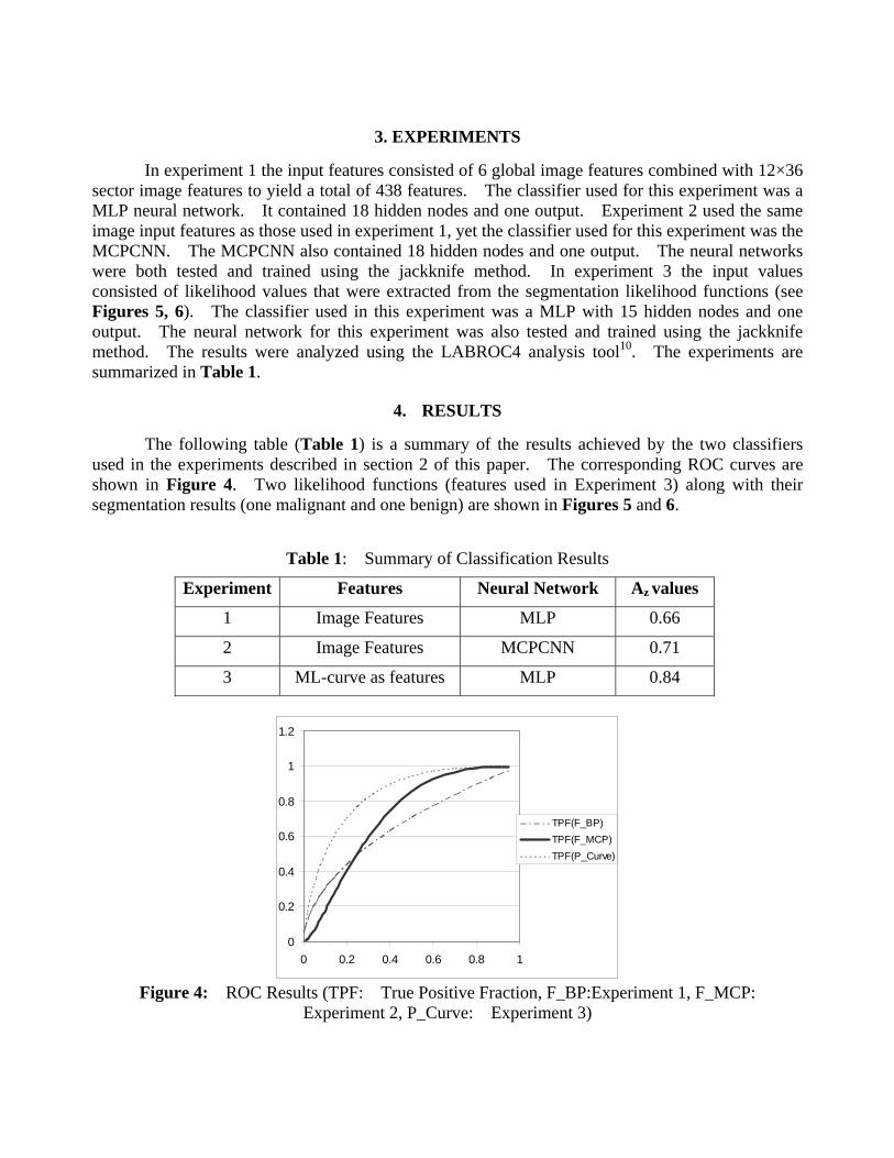
3. EXPERIMENTS

In experiment 1 the input features consisted of 6 global image features combined with 12×36 sector image features to yield a total of 438 features. The classifier used for this experiment was a MLP neural network. It contained 18 hidden nodes and one output. Experiment 2 used the same image input features as those used in experiment 1, yet the classifier used for this experiment was the MCPCNN. The MCPCNN also contained 18 hidden nodes and one output. The neural networks were both tested and trained using the jackknife method. In experiment 3 the input values consisted of likelihood values that were extracted from the segmentation likelihood functions (see Figures 5, 6). The classifier used in this experiment was a MLP with 15 hidden nodes and one output. The neural network for this experiment was also tested and trained using the jackknife method. The results were analyzed using the LABROC4 analysis tool10. The experiments are summarized in Table 1.

4. RESULTS

The following table (Table 1) is a summary of the results achieved by the two classifiers

used in the experiments described in section 2 of this paper. The corresponding ROC curves are shown in Figure 4. Two likelihood functions (features used in Experiment 3) along with their segmentation results (one malignant and one benign) are shown in Figures 5 and 6.

Table 1: Summary of Classification Results

Experiment Features Neural Network Az values

1 Image Features MLP 0.66

2 Image Features MCPCNN 0.71

3 ML-curve as features MLP 0.84

0

0.2

0.4

0.6

0.8

1

1.2

0 0.2 0.4 0.6 0.8 1

TPF(F_BP)TPF(F_MCP)TPF(P_Curve)

Figure 4: ROC Results (TPF: True Positive Fraction, F_BP:Experiment 1, F_MCP:

Experiment 2, P_Curve: Experiment 3)

Malignant Case (GUMC)

-840000

-830000

-820000

-810000

-800000

-790000

-780000

-770000

-7600002550 2600 2650 2700 2750 2800 2850 2900

intensity

likel

ihoo

d va

lues

Figure 5: The segmentation results for a malignant tumor. (a) likelihood function with respect to

threshold values for all segmentation steps (b) original image, (c) segmentation result

Benign Case (USF)

-880000

-878000

-876000

-874000

-872000

-870000

-868000

-866000

-8640002200 2250 2300 2350 2400 2450 2500

intensity

logv

alue

s

Figure 6: The segmentation results for a benign tumor. (a) likelihood function with respect to

threshold values for all segmentation steps (b) original image, (c) segmentation result

5. DISCUSSION OF RESULTS

n general there is a ma e likelihood function for

benign

performed better (see Figure 4) than the conventional neural network, where the

6. CONCLUSION

We found that the maximum likelihood mis an e

ACKNOWLEDGMENTS

This work was support by US Army Grant numbers DAMD17-00-1-0291 and DAMD17-01-1-0267

REFERENCES

. Byng JW, Boyd NF, Fishell E, Jong RA, Yaffe MJ, Automated analysis of mammographic

2. ings of the 3rd

3. st

I rked difference between the shape of th cases and the likelihood function for malignant cases (see Figures 5-6, i.e., the likelihood

functions for benign cases experience a sharp drop and the likelihood functions for malignant cases are smoother, overall. In the image, a sharp drop in likelihood value represents an abrupt change in segmented area. Overall MCPCNNAz value for Experiment 1 was 0.66, the Az value for Experiment 2 was 0.71 and the Az value for Experiment 3 was 0.84. The likelihood functions used as features provided the best diagnostic results, with regard to neural network performance. We believe that this phenomenon occurred because there is a clear difference between the appearance of the benign likelihood functions and the malignant likelihood functions. This may not be the case with regard to image features as some benign masses have malignant characteristics (e.g. - ill-defined borders) and vice versa. In future work we plan to find likelihood functions for various sectors, because we believe that certain sectors hold more valuable information than others. If we combine the feature information with likelihood functions found in the various sectors and use the MCPCNN, we could improve the performance in the classification of mammographic masses.

thod in conjunction with fuzzy shadow approach e

ffective approach for not only segmenting masses, but for also using its results to separate malignant and benign masses. Our method includes a fully-automated segmentation technique as well as the use of sector features that are designed for the separation of malignant and benign masses. We have also shown that the Multiple Circular Path Convolution Neural Network is better at separating malignant from benign masses and that the best classifier performance is achieved when the maximum likelihood features are used as inputs.

. The content of this paper does not necessarily reflect the position or policy of the government.

1densities, Physics in Medicine and Biology, 1996, vol. 41, pp. 909-923. Comer ML, Liu S, Delp EJ, Statistical Segmentation of Mammograms, ProceedInternational Workshop on Digital Mammography, Chicago, IL, June 9-12, 1996, pp. 475-478. Harvey JA, Fajardo LL, Innis, CA, Previous Mammograms in Patients with Impalpable BreaCarcinoma: Retrospective vs. Blinded Interpretation, American Journal of Roentgenology, 1993, vol. 161, pp. 1167-1172.

4. Heath M, Bowyer KW, Kopans D et al, Current status of the Digital Database for Screening Mammography}, Digital Mammography, Kluwer Academic Publishers, 1998, pp. 457-460.

5. Kinnard L, Lo S-C B, Wang P, Freedman MT, Chouikha M, Separation of Malignant and Benign Masses using a Maximum-Likelihood Analysis and Neural Networks, Proceedings of the SPIE Medical Imaging Conference, February, 2002, vol. 4684, part II, pp. 733-741.

6. Kinnard L, Lo S-C B, Wang P, Freedman MT, Chouikha M, Automatic Segmentation of Mammographic Masses Using Fuzzy Shadow and Maximum-Likelihood Analysis, Proceedings of the International Symposium on Biomedical Imaging (ISBI), July, 2002, pp. 241-244.

7. Lacey JV Jr, Devesa SS, Brinton LA, Recent trends in breast cancer incidence and mortality, 2002, vol. 39, no.2-3, pp. 82-88.

8. Martin JE, Moskowitz M, Milbrath JR, Breast Cancer Missed by Mammography, American Journal of Roengenology, 1979, vol. 132, pp. 737-739.

9. Lo SC, Li H, Wang J, Kinnard L, Freedman MT, A Multiple Circular Path Convolution Neural Network System for Detection of Mammographic Masses, IEEE Transactions on Medical Imaging, 2002, vol. 21, No. 2, pp. 150-158.

10. Metz C, LABROC Program, ftp://radiology.uchicago.edu/roc. 11. Meyer JE, Kopans DB, Stomper PC, Lindfors KK, Occult Breast Abnormalities: Percutaneous

Preoperative Needle Localization, Radiology, 1984, vol. 150, no. 2, pp. 335-337. 12. Qian W, Li L, Clarke LP, Image feature extration for mass detection in digital mammography:

Influence of wavelet analysis, 1999, Medical Physics, vol. 26, no. 3, pp. 402-408. 13. Rosenberg AL, Schwartz GF, Feig SA, Patchefsky AS, Clinically Occult Breast Lesions:

Localization and Significance, Radiology, 1987, vol. 162, no. 1, pp. 167-170. 14. Sahiner B, Chan H-P, Wei D, Petrick N, Helvie MA, Adler DD, Goodsit MM, Image feature

selection by a genetic algorithm: Application to classification of mass and normal breast tissue, Medical Physics, 1996, vol. 23, no. 10, pp. 1671-1684.

15. Sahiner B, Chan H-P, Petrick N, Helvie MA, Hadjiiski LM, Improvement of mammographic mass characterization using spiculation measures and morphological features, Medical Physics, 2001, vol.28, no. 7, pp. 1455-1465.

16. Wei D, Chan H-P, Helvie MA, Sahiner B, Petrick N, Adler DD, Goodsitt MM, False-positive reduction technique for detection of masses on digital mammograms: Global and local multiresolution texture analysis, Medical Physics, 1997, vol. 24, no. 6, pp. 903-914.

17. Yankaskas BC, Knelson MH, Abernethy ML, Cuttino JT, Clark RL, Needle Localization Biopsy of Occult Lesions of the Breast, vol. 23, no. 10, pp. 729-733.

LIKELIHOOD FUNCTION ANALYSIS FOR SEGMENTATION OF MAMMOGRAPHIC MASSES FOR VARIOUS MARGIN GROUPS

Lisa Kinnarda,b,c, Shih-Chung B. Loa, Erini Makarioua, Teresa Osickaa,d, Paul Wangc,

Matthew T. Freedmana, Mohamed Chouikhab

aISIS Center, Dept. of Radiology, Georgetown University Medical Center, Washington, D.C., USA bDepartment of Electrical and Computer Engineering, Howard University, Washington, D.C., USA

cBiomedical NMR Laboratory, Department of Radiology, Howard University, Washington, D.C., USA

dDepartment of Electrical Engineering and Computer Science, The Catholic University of America, Washington DC, USA

ABSTRACT The purpose of this work was to develop an automatic boundary detection method for mammographic masses and to observe the method’s performance on different four of the five margin groups as defined by the ACR, namely, spiculated, ill-defined, circumscribed, and obscured. The segmentation method utilized a maximum likelihood steep change analysis technique that is capable of delineating ill-defined borders of the masses. Previous investigators have shown that the maximum likelihood function can be utilized to determine the border of the mass body. The method was tested on 122 digitized mammograms selected from the University of South Florida’s Digital Database for Screening Mammography (DDSM). The segmentation results were validated using overlap and accuracy statistics, where the gold standards were manual traces provided by two expert radiologists. We have concluded that the intensity threshold that produces the best contour corresponds to a particular steep change location within the likelihood function.

1. INTRODUCTION In a CADx system, segmentation is arguably one of the most important aspects – particularly for masses – because strong diagnostic predictors for masses are shape and margin type [2,9]. The margin of a mass is defined as the interface between the mass and surrounding tissue [2]. Furthermore, breast masses can have unclear borders and are sometimes obscured by glandular tissue in mammograms. A spiculated mass consists of a central mass body surrounded by fibrous projections, hence the resulting stellate shape. For the aforementioned reasons, proper segmentation - to include the body and periphery - is extremely important and is essential for the computer to analyze, and in turn, determine the malignancy of the mass in mammographic CADx systems. Over the years researchers have used many methods to segment masses in mammograms. Petrick [7] et al. developed the Density Weighted Contrast Enhancement (DWCE) method, in which series of filters are applied to the image in an attempt to extract masses. Comer et al. [1] segmented digitized mammograms into

homogeneous texture regions by assigning each pixel to one of a set of classes such that the number incorrectly classified pixels was minimized via Maximum Likelihood (ML) analysis. Li [5] developed a method that employs k-means classification to classify pixels as belonging to the region of interest (ROI) or background. Kupinski and Giger developed a method [4], which uses ML analysis to determine final segmentation. In their method, the likelihood function is formed from likelihood values determined by a set of image contours produced by the region growing method. This method is a highly effective one that was also implemented by Te Brake and Karssemeijer in their comparison between the discrete dynamic contour model and the likelihood method [9]. For this reason we chose to investigate its use as a possible starting point from which a second method could be developed. Consequently in our implementation of this work we discovered an important result, i.e., the maximum likelihood steep change. It appears that in many cases this method produces contour choices that encapsulate important borders such as mass spiculations and ill-defined borders.

2. METHODS

2.1 Initial Contours As an initial segmentation step, we followed the overall region similarity concept to aggregate the area of interest [1, 4]. Used alone, a sequence of contours representing the mass is generated; however, the computer is not able to choose the contour that is most closely correlated with the experts’ delineations. Furthermore, we have devised an ML function steep change analysis method that chooses the best contour that delineates the mass body as well as its extended borders, i.e., extensions into spiculations and areas in which the borders are ill-defined or obscured. This method is an extension of the method developed by Kupinski and Giger [4] that uses ML function analysis to select the contour which best represents the mass, as compared to expert radiologist traces. We have determined that this technique can select the contour that accurately represents the mass body contour for a given set of parameters; however, further analysis of the likelihood function revealed that the computer could

1130-7803-8388-5/04/$20.00 ©2004 IEEE

choose a set of three segmentation contour choices from the entire set of contour choices, and then make a final decision from these three choices. The algorithm can be summarized in several steps. Initially, we use an intensity based thresholding scheme to generate a sequence of grown contours (Si), where gray value is the similarity criterion. The image is also multiplied by a 2D trapezoidal membership function (2D shadow), whose upper base measures 40 pixels and lower base measures 250 pixels (1 pixel = 50 microns). The image to which the shadow has been applied is henceforth referred to as the "fuzzy" image. The original image and its fuzzy version were used to compute the likelihood of the mass’s boundaries. The computation method is comprised of two components for a given boundary: (1) formulation of the composite probability and (2) evaluation of likelihood. In addition, we chose to aggregate contours using the original image. This accounts for the major difference from that implemented by the previous investigators. Since smoother contours were not used, the likelihood function showed greater variations. In many situations, the greatest variations occurred when there was a sudden increase of the likelihood, and this was strongly correlated with the end of the mass border growth. This phenomenon would be suppressed if the fuzzy image was used to generate the contours. The fuzzy image was used mainly to construct the likelihood function. 2.2 Composite Probability Formation For a contour (Si), the composite probability (Ci) is calculated: ( )( ) ( )( )iiiiii SyxmpSyxfpSC ,, ×= (1)

The quantity fi(x,y) is the area to which the 2D shadow has been multiplied, p(fi(x,y)|Si) is the probability density function of the pixels inside Si where ‘i’ is the region growing step associated with a given intensity threshold. The quantity mi(x,y) is the area outside Si (non-fuzzy), and p(mi(x,y)|Si) is the probability density function of the pixels outside Si. Next we find the logarithm of the composite probability of the two regions, Ci:

( ) ( )( )( ) ( )( )( )iiiiii SyxmpSyxfpSCLog ,log,log += (2)

2.3 Evaluation of Likelihood Function The likelihood that the contour represents the fibrous portion of the mass, i.e., mass body is determined by assessing the maximum likelihood function:

( )( ) niSSCLog iii ,...1,;maxarg = (3)

Equation (3) intends to find the maximum value of the aforementioned likelihood values as a function of intensity threshold. It has been assessed (also by other investigators [4]) that the intensity value corresponding to this maximum likelihood value is the optimal intensity needed to delineate the mass body contour. However, in our implementation it was discovered that the intensity threshold corresponding to the maximum likelihood value confines the contour to the mass body. In our study many of these contours did not include the extended borders. We, therefore, hypothesize that the contour represents the mass’s extended borders may well be determined by assessing the maximum changes of the likelihood function, i.e., locate the steepest likelihood value changes within the function:

( )( ) niSSCLogdi

diii ,,1,; K= (4)

Based on this assumption, we have carefully analyzed the behavior of maximum likelihood function. The analysis reveals that we have successfully discovered that the most accurate mass delineation is usually obtained by using the intensity value corresponding to the first or second steep change locations within the likelihood function immediately following the maximum likelihood value on the likelihood function.

-735000

-730000

-725000

-720000

-715000

-710000

-705000

-700000

2600 2650 2700 2750 2800 2850

Figure 1: A likelihood function with steep change indicators

2.4 Steep change definition The term "steep change" is rather subjective and can defined as a location between two or more points in the function where the likelihood values experience a significant change. In some cases the likelihood function increases at a slow rate. The algorithm design accounts for this issue by calculating the difference between likelihood values in steps over several values and comparing the results to two thresholds. The difference equation is given by:

( ) ( ) ( )( ) Nttwzfwtzfth ,,0,1 K=+−−−= (5)

where f is the likelihood function, z is the maximum intensity, w is the width of the interval over which the likelihood differences are calculated (e.g. – for w=7 differences are calculated every 7 points), and N is the total number of points in the searchable area divided by w. If the calculation in question yields a value greater than or equal to a given threshold, then the intensity corresponding to this location is considered to be a steep change location. The threshold algorithm occurs as follows: If (h(t)ML > MLT1); t=0,…,m Then choice 1 = intensity where that condition is satisfied If (h(t)ML > MLT2); t=m,…,z Then choice 2 = intensity where that condition is satisfied where h(t)ML is the steep change value given by equation (5), MLT1 and MLT2 are pre-defined threshold values, m is the location in the function where the choice 1 condition is satisfied, and z is the location in the function where the choice 2 condition is satisfied. Once the condition is satisfied for the first threshold value (MLT1) then its corresponding intensity value is used to produce the segmentation contour for the first steep change location. Once the condition is satisfied for MLT2 then its corresponding intensity value is used to produce the segmentation contour for the second steep change location. 2.5 Validation The segmentation method was validated on the basis of overlap and accuracy [8,10]:

FPTPFN

TP

NNN

NOverlap

++= (6)

Group 2 (first steep change location)

Group 1 (max likelihood location)

Group 3 (second steep change location)

114

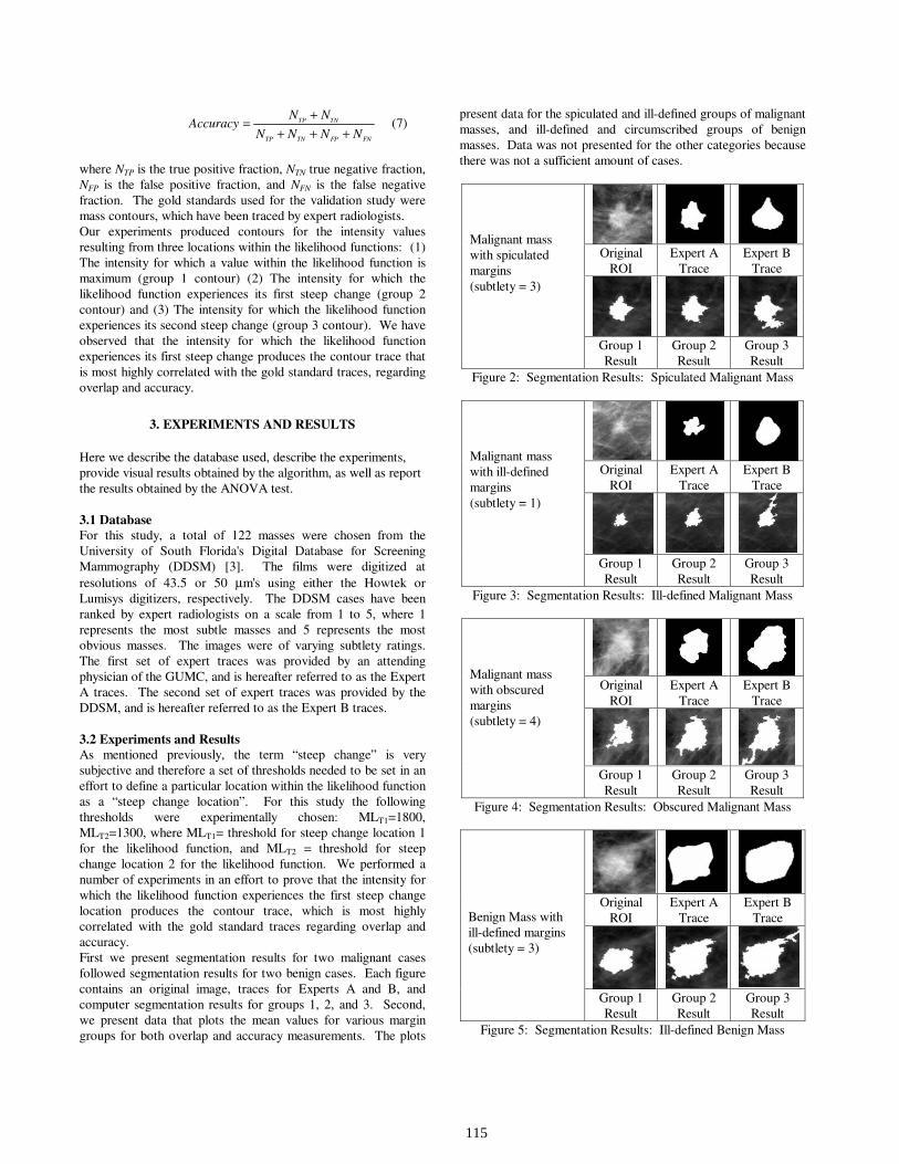
FNFPTNTP

TNTP

NNNN

NNAccuracy

++++= (7)

where NTP is the true positive fraction, NTN true negative fraction, NFP is the false positive fraction, and NFN is the false negative fraction. The gold standards used for the validation study were mass contours, which have been traced by expert radiologists. Our experiments produced contours for the intensity values resulting from three locations within the likelihood functions: (1) The intensity for which a value within the likelihood function is maximum (group 1 contour) (2) The intensity for which the likelihood function experiences its first steep change (group 2 contour) and (3) The intensity for which the likelihood function experiences its second steep change (group 3 contour). We have observed that the intensity for which the likelihood function experiences its first steep change produces the contour trace that is most highly correlated with the gold standard traces, regarding overlap and accuracy.

3. EXPERIMENTS AND RESULTS

Here we describe the database used, describe the experiments, provide visual results obtained by the algorithm, as well as report the results obtained by the ANOVA test. 3.1 Database For this study, a total of 122 masses were chosen from the University of South Florida's Digital Database for Screening Mammography (DDSM) [3]. The films were digitized at resolutions of 43.5 or 50 µm's using either the Howtek or Lumisys digitizers, respectively. The DDSM cases have been ranked by expert radiologists on a scale from 1 to 5, where 1 represents the most subtle masses and 5 represents the most obvious masses. The images were of varying subtlety ratings. The first set of expert traces was provided by an attending physician of the GUMC, and is hereafter referred to as the Expert A traces. The second set of expert traces was provided by the DDSM, and is hereafter referred to as the Expert B traces. 3.2 Experiments and Results As mentioned previously, the term “steep change” is very subjective and therefore a set of thresholds needed to be set in an effort to define a particular location within the likelihood function as a “steep change location”. For this study the following thresholds were experimentally chosen: MLT1=1800, MLT2=1300, where MLT1= threshold for steep change location 1 for the likelihood function, and MLT2 = threshold for steep change location 2 for the likelihood function. We performed a number of experiments in an effort to prove that the intensity for which the likelihood function experiences the first steep change location produces the contour trace, which is most highly correlated with the gold standard traces regarding overlap and accuracy. First we present segmentation results for two malignant cases followed segmentation results for two benign cases. Each figure contains an original image, traces for Experts A and B, and computer segmentation results for groups 1, 2, and 3. Second, we present data that plots the mean values for various margin groups for both overlap and accuracy measurements. The plots

present data for the spiculated and ill-defined groups of malignant masses, and ill-defined and circumscribed groups of benign masses. Data was not presented for the other categories because there was not a sufficient amount of cases.

Original

ROI Expert A

Trace Expert B

Trace

Malignant mass with spiculated margins (subtlety = 3)

Group 1 Result

Group 2 Result

Group 3 Result

Figure 2: Segmentation Results: Spiculated Malignant Mass

Original

ROI Expert A

Trace Expert B

Trace

Malignant mass with ill-defined margins (subtlety = 1)

Group 1 Result

Group 2 Result

Group 3 Result

Figure 3: Segmentation Results: Ill-defined Malignant Mass

Original

ROI Expert A

Trace Expert B

Trace

Malignant mass with obscured margins (subtlety = 4)

Group 1 Result

Group 2 Result

Group 3 Result

Figure 4: Segmentation Results: Obscured Malignant Mass

Original

ROI Expert A

Trace Expert B

Trace

Benign Mass with ill-defined margins (subtlety = 3)

Group 1 Result

Group 2 Result

Group 3 Result

Figure 5: Segmentation Results: Ill-defined Benign Mass

115

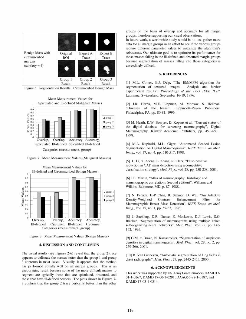
Original

ROI Expert A

Trace Expert B

Trace

Benign Mass with circumscribed margins (subtlety = 4)

Group 1 Result

Group 2 Result

Group 3 Result

Figure 6: Segmentation Results: Circumscribed Benign Mass

Mean Measurement Values for Spiculated and Ill-Defined MalignantMasses

00.10.20.30.40.50.60.70.80.9

1

(overlap,spiculated)

(overlap, ill-defined)

(accuracy,spiculated)

(accuracy, ill-defined)

Categories (measurement, margin group)

Mea

n V

alue

s (r

ange

, 0-1

)

group 1

group 2

group 3

Figure 7: Mean Measurement Values (Malignant Masses)

0

0.1

0.2

0.3

0.4

0.5

0.6

0.7

0.8

0.9

1

benign (overlap,ill-defined)

benign (overlap,circumscribed)

benign(accuracy, ill-

defined)

benign(accuracy,

circumscribed)

group 1

group 2

group 3

Figure 8: Mean Measurement Values (Benign Masses)

4. DISCUSSION AND CONCLUSION

The visual results (see Figures 2-6) reveal that the group 2 trace appears to delineate the masses better than the group 1 and group 3 contours in most cases. Visually, it appears that the method has performed equally well on all margin groups. This is an encouraging result because some of the more difficult masses to segment are typically those that are spiculated, obscured, and those that have ill-defined borders. The plots shown in Figures 7-8 confirm that the group 2 trace performs better than the other

groups on the basis of overlap and accuracy for all margin groups, therefore supporting our visual observations. In future work, a worthwhile study would be to test gather more data for all margin groups in an effort to see if the various groups require different parameter values to maximize the algorithm’s robustness. Our ultimate goal is to optimize its performance for those masses falling in the ill-defined and obscured margin groups because segmentation of masses falling into those categories is exceedingly difficult.

5. REFERENCES [1] M.L. Comer, E.J. Delp, “The EM/MPM algorithm for segmentation of textured images: Analysis and further experimental results”, Proceedings of the 1995 IEEE ICIP, Lausanne, Switzerland, September 16-19, 1996. [2] J.R. Harris, M.E. Lippman, M. Morrow, S. Hellman, “Diseases of the breast”, Lippincott-Raven Publishers, Philadelphia, PA, pp. 80-81, 1996.

[3] M. Heath, K.W. Bowyer, D. Kopans et al., “Current status of the digital database for screening mammography”, Digital Mammography, Kluwer Academic Publishers, pp. 457-460 , 1998. [4] M.A. Kupinski, M.L. Giger, “Automated Seeded Lesion Segmentation on Digital Mammograms”, IEEE Trans. on Med. Imag., vol. 17, no. 4, pp. 510-517, 1998. [5] L. Li, Y. Zheng, L. Zhang, R. Clark, “False-positive reduction in CAD mass detection using a competitive classification strategy”, Med. Phys., vol. 28, pp. 250-258, 2001. [6] J.E. Martin, “Atlas of mammography: histologic and mammographic correlations (second edition)”, Williams and Wilkins, Baltimore, MD, p. 87, 1988. [7] N. Petrick, H-P Chan, B. Sahiner, D. Wei, “An Adaptive Density-Weighted Contrast Enhancement Filter for Mammographic Breast Mass Detection”, IEEE Trans. on Med. Imag., vol. 15, no. 1, pp. 59-67, 1996. [8] J. Suckling, D.R. Dance, E. Moskovic, D.J. Lewis, S.G. Blacker, “Segmentation of mammograms using multiple linked self-organizing neural networks”, Med. Phys., vol. 22, pp. 145-152, 1995. [9] G.M. te Brake, N. Karssemeijer, “Segmentation of suspicious densities in digital mammograms”, Med. Phys., vol. 28, no. 2, pp. 259-266, 2001. [10] B. Van Ginneken, “Automatic segmentation of lung fields in chest radiographs”, Med. Phys., 27, pp. 2445-2455, 2000.

6. ACKNOWLEDGMENTS

This work was supported by US Army Grant numbers DAMD17-01-1-0267, DAMD 17-00-1-0291, DAAG55-98-1-0187, and DAMD 17-03-1-0314.

Mean Measurement Values for Spiculated and Ill-defined Malignant Masses

Mea

n V

alue

s

Mea

n V

alue

s

Mean Measurement Values for Ill-defined and Circumscribed Benign Masses

Categories (measurement, group)

Overlap, Spiculated

Overlap, Ill-defined

Accuracy, Spiculated

Accuracy, Ill-defined

Overlap, Ill-defined

Overlap, Circumsc.

Accuracy, Ill-defined

Accuracy, Circumsc.

Categories (measurement, group)

116

Changes in biophysical parameters of plasma membranes influence

cisplatin resistance of sensitive and resistant epidermal carcinoma cells

Xing-Jie Liang,a Jun-Jie Yin,b Jien-Wei Zhou,c Paul C. Wang,c

Barbara Taylor,a Carol Cardarelli,a Michael Kozar,d Raynard Forte,d

Adorjan Aszalos,a and Michael M. Gottesmana,*

aLaboratory of Cell Biology, National Cancer Institute, National Institutes of Health, Bethesda, MD 20892-4254, USAb Instrumentation and Biophysics Branch, Center for Food Safety and Applied Nutrition, Food and Drug Administration,

College Park, MD 20740-3835, USAcDepartment of Radiology, Howard University, Washington, DC 20060, USA

dDivision of Experimental Therapeutics, Walter Reed Army Institute of Research, Silver Spring, MD 20910, USA

Received 30 June 2003, revised version received 15 September 2003

Abstract

The mechanism of resistance of cancer cells to the anticancer drug cisplatin is not fully understood. Using cisplatin-sensitive KB-3-1 and -

resistant KCP-20 cells, we found that the resistant cells have higher membrane potential, as determined by membrane potential sensing oxonol

dye. Electron spin resonance and fluorescence polarization studies revealed that the resistant cells have more ‘‘fluid’’ plasma membranes than

the sensitive cells. Because of this observed difference in membrane ‘‘fluidity,’’ we attempted modification of the plasma membrane fluidity by

the incorporation of heptadecanoic acid into KB-3-1 and KCP-20 cell membranes. We found that such treatment resulted in increased

heptadecanoic acid content and increased fluidity in the plasma membranes of both cell types, and also resulted in increased cisplatin resistance

in the KCP-20 cells. This finding is in accord with our results, which showed that the cisplatin-resistant KCP-20 cells have more fluid

membranes than the cisplatin-sensitive KB-3-1 cells. It remains to be determined whether the observed differences in biophysical status and/or

fatty acid composition alone, or the secondary effect of these differences on the structure or function of some transmembrane protein(s), is the

reason for increased cisplatin resistance.

D 2003 Elsevier Inc. All rights reserved.

Keywords: Cisplatin resistance; Heptadecanoic acid; Plasma membrane fluidity; Membrane potential; Fluorescence polarization; Human epidermal carcinoma

KB cells

Introduction

Cis-diamminodichloroplatinum II (cisplatin) is one of

the most useful anticancer drugs. Treatment protocols for

solid tumors of the esophagus, bladder, ovary, testes, head,

and neck include this drug. As for most antitumor agents,

resistance develops in cancer cells, limiting their efficacy.

The reason for resistance against cisplatin is not fully

understood. Several mechanisms have been suggested,

including decreased cisplatin accumulation [1,2], and alter-

ation of apoptotic signaling [3,4]. Reports also indicate that

alterations in growth regulating proteins, such as c-Myc

[5], inhibition of caspase-9 [6], and reduced inhibition of

DNA synthesis [7] are associated with cisplatin resistance.

Involvement of plasma membrane lipids in cisplatin resis-

tance has also been implicated [8]. Britz et al. [9] suc-

ceeded in decreasing cisplatin resistance by treating

monoclonal cells with a free or liposome-encapsulated bile

acid derivative.

Our interest was focused on the biophysical status of

plasma membranes in relation to cisplatin resistance. We

investigated the biophysical differences between cisplatin-

resistant and -sensitive cells and the influence of a fatty acid

inserted into the plasma membranes on cisplatin sensitivity

of human epidermal carcinoma KB cells.

0014-4827/$ - see front matter D 2003 Elsevier Inc. All rights reserved.

doi:10.1016/j.yexcr.2003.10.012

* Corresponding author. Laboratory of Cell Biology, Center for Cancer

Research, National Cancer Institute, National Institutes of Health, Room 1A-

09, 37 Convent Drive, Bethesda, MD 20892-4254. Fax: +1-301-402-0450.

E-mail address: mgottesman@nih.gov (M.M. Gottesman).

www.elsevier.com/locate/yexcr

Experimental Cell Research 293 (2004) 283–291

Materials and methods

Cell lines

The KB-3-1 cell line was derived from a single clone of

human KB epidermal carcinoma cells (a HeLa subclone),

after two subclonings, as described by Akiyama et al. [10].

The cisplatin-resistant subline of KB-3-1 cells was selected

by exposure to 0.5 Ag/ml cisplatin (KB-CP.5) for 42 days.

After that, single clones were picked and propagated in

medium containing 0.5 Ag/ml cisplatin. One other cisplatin-

resistant cell line, KCP-20, was obtained after 6 months’

exposure of KB-3-1 cells to increasing concentrations of

cisplatin, up to 20 Ag/ml [11]. KCP-20 cells were maintained

in medium containing 5 Ag/ml cisplatin and taken out of

cisplatin before making the measurements. All cell lines were

grown in Dulbecco’s modified Eagle medium (Invitrogen,

Grand Island, NY), supplemented with L-glutamine, penicil-

lin, streptomycin (Quality Biological, Gaithersburg, MD),

and 10% fetal bovine serum (Whittaker Bioproducts, Wal-

kersville, MD).

Membrane potential measurements

Membrane potential measurements were performed by

flow cytometry, using the negatively charged DiBaC4 (3)

oxonol dye (Molecular Probes, Eugene, OR), essentially as

described earlier [12]. Briefly, a cell suspension of 1 � 106

cells/ml was equilibrated for 1 min in PBS followed by the

addition of oxonol dye, 150 M. After exactly 2 min

equilibration at room temperature, histograms were collect-

ed from 104 cells. Reproducibility was determined by

measuring membrane potentials of the cells on different

days, from separate cultures, and by comparing the relative

fluorescence of the oxonol-stained cell types.

Oxonol fluorescence intensity measures membrane po-

tential when the extracellular potassium concentration is

changed from 5 to 150 mM, resulting in increased fluores-

cence intensity of the oxonol-stained cells and thus making

the cells depolarized. All measurements were made with a

Becton Dickinson FACSCalibur flow cytometer (Becton

Dickinson, Mountain View, CA), operated with a 15-mW

argon ion laser tuned to 488-nm excitation wavelength.

Fluorescence emission was collected at 525 nm. Results are

expressed in comparative histograms of representative series.

Polarity of fluorescent membrane probes in live cells

Measurements of steady-state fluorescence polarization

were done with a spectrofluorometer LS50B (Perkin Elmer,

Norwalk, CT) and the lipid-soluble fluorophore, 1-(4-trime-

thylammoniumphenyl)-6-phenyl-1,3,5-hexatriene (TMA-

DPH) (Molecular Probes). This fluorophore is known to

probe plasma membranes of cells at the surface. TMA-DPH

was dissolved in tetrahydrofurane at a concentration of 2

mM and was kept in the dark at 4jC. Cells (106/ml) were

labeled with TMA-DPH at a concentration of 2 AM in PBS.

After 10 min incubation time at 4jC, the cell suspension

was centrifuged and washed two times in the centrifuge with

PBS. After resuspension in PBS, fluorescence anisotropy

was measured at 25jC. The excitation wavelength was 355

nm and the emission was measured at 430 nm with a slit

width of 5. Polarization values were calculated according to

Collins and Scott [13] by the equation P = (I0,0 � G * I0,90) /

(I0,0 + G * I0,90) from the measured fluorescence intensities.

Electron spin resonance (ESR) studies on live cells

ESR studies were conducted with 5-doxyl stearic acid (5-

doxyl-SA) and with 2,2,6,6-tetramethyl piperidin-1-oxyl-4-

yl-octadecenoate (T-SASL) probes (Molecular Probes). The

first probe intercalates to the 5 carbon depth in the outer

leaflet of the plasma membrane [14] and T-SASL at the

surface of the plasma membranes [15]. Labeling the cells

with the spin probes was done as follows: 5-doxyl-SA was

dissolved in ethanol, 1 mg/ml, and was kept at 4jC. Then, 1�107 cells were mixed with 8� 10�8 mol spin label in 0.02 ml

volume of PBS. After 1 min contact time, the cell suspension

was transferred into a 50-Al micropipette capillary tube and

sealed at the bottomwith Critoseal (Syva Co., Palo Alto, CA).

The micropipette with the cells was placed into the cavity of a

Varian E-9 Century series spectrometer (Syva Co.). ESR

spectra were recorded at X-band, at 9.5 kHz, 100-field

modulation, 4-Gous modulation amplitude, 100-Gous sweep

range, and at 10 mW microwave power. The temperature of

the probe was set to 24jC by the variable temperature

accessory using N2 gas flow. Evaluation of the obtained

ESR spectra, when 5-doxyl-SAwas used, was by the equation

expressing the order parameter S:

S ¼ 0:5407 ðT11 � T1Þ=a0; where a0 ¼ ðT11 þ 2T1Þ=3

and T11 and T1 are the outer and inner tensors obtained from

the ESR spectra.

When the T-SASL probe was used, the same instrument

parameters were applied, except that the incident microwave

power was 20 mW. The spectral parameters, h0 and h�1 are

the spectral amplitudes and the ratio h0/h�1 defines the

motional freedom of the probe according to Yin et al. [15].

With both spin labels, the ESR spectra show contribution

from spin labels of restricted motion with no contribution

from the free-moving spin label.

Lipid packing of plasma membranes in live cells

Plasma membrane lipid packing can be studied by insert-

ing the fluorescence probe merocyanine 540 (MRC 540)

(Molecular Probes) into cell membranes and assessing the

degree of insertion by fluorescence intensity measurement,

using flow cytometry [16,17]. The experiment was according

to Schlegel et al. [16] with some modifications. Briefly, 1 �107 cells, suspended in 1 ml of PBS were treated with 10 Al of

X.-J. Liang et al. / Experimental Cell Research 293 (2004) 283–291284

a MC540 stock solution of 1 mg/ml, in 60% ethanol, 40%

water. After a 10-min incubation at room temperature, cells

were pelleted in a centrifuge, washed once in PBS by

centrifugation, resuspended in 1 ml PBS, and fluorescence

histogramswere obtained. ABectonDickinson FACSCalibur

flow cytometer (Becton Dickinson, Franklin Lakes, NJ) was

used at 488-nm excitation and 575-nm emission wavelength.

Histograms were collected with 104 cells. Results are

expressed as means of fluorescence of the histograms

obtained from duplicate measurements of one typical set of

cells.

Preparation of cells for NMR spectrometry

KB-3-1 and KCP-20 cells were grown to 90% conflu-

ence, harvested with 0.05% trypsin, 0.53 AM EDTA, centri-

fuged at 4jC at 730 � g for 10 min, and washed twice with

growth medium. To perform a long-term NMR study, the

cells were restrained in an agarose thread [18,19]; 0.5 ml of

(9 � 107 cells) was mixed with an equal volume of liquid

agarose in phosphate-buffered saline, and immersed in a

bath at 37jC for 5–7 min. The mixture was extruded under

low pressure through cooled tubing (0.5 mm ID) into a 10-

mm NMR tube containing growth medium. Using 0.5-mm

threads ensures that there is no metabolic compromise, and

the cells are viable and in stable energetic status for a long

period of time, while the threads maintain their mechanical

strength. The gel threads, which fill the tube, are concen-

trated without compression at the bottom of the NMR tube

by insertion of a plastic insert with the perfusion fitting. A

Teflon inflow tube (0.5 mm ID) was placed near the bottom

of the tube. The gel threads were perfused with growth

medium at 0.9 ml/min. Cells were continuously perfused for

more than 40 h. Accumulation of data was started within 30

min after the harvest.

NMR spectrometry of live cells

The 31P NMR spectra were recorded at 37jC on a Varian

XL-400 machine (Varian Associates, Inc., Palo Alto, CA) at

162 MHz using RF pulse corresponding to a 72j flip angle

and 2 s repetition time. The flip angle used was the Ernst

angle for phosphocreatine (PCr) (T1 relaxation time, 3 s).

There were more than 40 spectra obtained. Each spectrum

contained 1800 transients and took 1 h. During the entire

study, the system was deuterium locked with an external

source (99.9% D2O in a capillary, Sigma, St. Louis, MO) to

avoid magnetic field drift.

All the spectra were transformed and viewed separately to

confirm that the spectra did not change during the experi-

ment. There were 25,000 data points collected and zero-

filled to 8k before Fourier transformation. The spectra were

added and 10-Hz line broadening was applied to obtain Fig.

3. The chemical shifts were standardized to h-adenosinetri-phosphate (h-ATP) set to �18.70 ppm. Many phosphorus

metabolites were identified, including phosphocholine (PC,

3.57 ppm), inorganic phosphate (Pi, 2.59 ppm), glycero-

phosphoethanolamine (GPE, 0.81 ppm), glycerophospho-

choline (GPC, 0.26 ppm), phosphocreatine (PCr, �2.69

ppm), g-adenosine triphosphate (g-ATP, �5.12 ppm), a-adenosine triphosphate (a-ATP, �10.19 ppm), and diphos-

phodiesters (dPdE, �10.86, �12.58 ppm). Chemical shifts

of these molecules are also listed in the literature [18,19].

Treatment of cells with heptadecanoic acid and cell

proliferation studies

Treatment of KB-3-1 and KCP-20 cells with heptadeca-

noic acid was carried out in 24-well plates (Corning Inc.,

Corning, NY), with modification of the method used by

Callaghan et al. [20]. After exploratory dose selection studies

for cisplatin and heptadecanoic acid, the final conditions

were as follows: cells (106/ml) were incubated in appropriate

medium, as described above for both cell types, and after 2–

3 days of incubation, the medium was withdrawn and

replaced by serum-free medium. Following 6 h incubation

at 37jC, 5% CO2 medium was replaced by serum-free

medium containing different concentrations of heptadeca-

noic acid or nothing. This incubation was followed by

replacement of the medium with complete medium contain-

ing cisplatin or nothing. KB-3-1 cells were treated with 0.08

Ag/ml and KCP-20 cells with 5 Ag/ml cisplatin from a stock

solution of 500 Ag/ml aqueous solution. Cells were harvested

after 5–6 days’ incubation and treated with heptadecanoic

acid alone, with cisplatin alone, heptadecanoic acid plus

cisplatin or nothing, and were counted after trypsinization by

a Coulter Particle Counter (Coulter Electronics, Luton, UK).

Calculation of proliferation was based on cells treated with

nothing as 100%. The expected yield was: cell count of cells

treated with heptadecanoic acid alone multiplied by cell

count of cells treated with cisplatin alone. The cell count

of cells treated with both reagents was then related to the

previous cell count product and tabulated.

Preparation of plasma membranes for determination of

relative fatty acid composition

For the purpose of plasma membrane preparation, 107

cells from each cell line were harvested at log phase and

washed with ice-cold PBS. Cells were sedimented by

centrifugation and then suspended in ice-cold hypotonic

solution (0.5 mM KH2PO4, 0.1 mM EDTA containing 1%

protease inhibitor aprotonin, pH 8.0) for 5 min. Cells were

disrupted on ice by a tight Dounce homogenizer with

constant 40 strokes. Samples were checked for complete

disruption in a phase-contrast microscope. Homogenates

were centrifuged at 2000 � g for 10 min at 4jC to discard

the nuclei and then the supernatant was centrifuged at

25,000 � g for 25 min to pellet all other organelles. The

resulting supernatant was further centrifuged for 55 min at

4jC. The membranes sedimented at the bottom and were

stored at �80jC before fatty acid analysis. To determine

X.-J. Liang et al. / Experimental Cell Research 293 (2004) 283–291 285

that the sediment contained only plasma membranes and no

membranes of organelles, markers were used in connection

with Western blot analyses. For a positive marker, the anti-

integrin antibody anti-2/VLA-2a was used according to

Emsley et al. [21].

Conversion of plasma membrane lipids to methyl esters and

fatty acid analysis

Fats were extracted into organic phase by vortexing the

membrane preparations obtained as described above, with

minor modification of the methods of Kozar et al. [22]. In

brief, 2 ml of HPLC-grade water (Fisher Scientific, Pitts-

burgh, PA) was added to the membranes together with 3.75

ml of 2:1 (v/v) methanol/chloroform (Fisher Scientific) and

the suspension was vortexed for 15 min. Then, after addition

of 1 ml chloroform and 1 min vortexing, the suspension was

centrifuged for 10 min at 2000 rpm. The separated organic

phase was dried in an N2 stream and heated in 1 ml 2 M

methanolic HCl [11 ml methanol with dropwise addition of

2.5 ml acetyl chloride (Sigma)] at 85jC for 18 h in a screw-

capped tube. The fatty acid methyl esters which formed were

then extracted into heptane for GC-MS analysis. Samples

were analyzed on a Hewlett-Packard 6890 plus GC equipped

with 7683 auto-injector. The injection port was held at

constant 280jC with 2 Al injected in the spitless mode onto

a DB-5 ms capillary column with 30 m � 0.25 mm ID �0.25 Am film thickness (J&W Scientific, Folsom, CA). Initial

oven temperature was 80jC with a ramp of 40jC/min to a

final temperature of 290jC and hold for 0.75 min. Helium

was used as the carrier gas at a constant velocity of 41 cm/s.

Electron impact ionization at 70 eV was performed using

standard autotune conditions. The source temperature was

maintained at 230jC while the quadrupoles were maintained

at 150jC. FAMEs were analyzed in full scan mode for

qualitative identification as well as in selected ion monitor-

ing mode for ratio determination. Location of the analyzed

two fatty acids in the obtained chromatograms was ascer-

tained by standards of hexa- and heptadecanoic acid methyl

esters (Sigma). The ratio of heptadecanoic acid to hexade-

canoic acid methyl esters was determined since heptadeca-

noic acid was used to treat the cells and the hexadecanoic

acid content of cells was assumed to be constant. This ratio is

defined as the area under the peak for hexadecanoic acid/area

under the peak for heptadecanoic acid methyl esters.

Visualization of distribution of K+ channels in cells by

immunofluorescence microscopy

For visualization of distribution of K+ channels in cells,

cells were grown on 189-mm glass coverslips in petri

dishes. Cells were fixed with 3.5% formaldehyde in PBS

for 10 min, followed by 0.1% Triton X-100 treatment for 5

min for permeabilization. After washing, cells were treated

with 3% BSA in PBS for 30 min and subsequently treated

with the primary antibody (Ab) for 1 h. The Ab was TW1K-

2 (P-19) goat polyclonal Ab (Santa Cruz Biotechnology,

Santa Cruz, CA). After five washings, cells were incubated

with CyTM3-conjugated affinity pure donkey anti-goat,

secondary Ab (1:100 dilution) (Jackson Immuno-research

Laboratory). Cells were washed extensively after the sec-

ondary Ab treatment. The slides with the treated cells were

mounted on microscope slides with fluorescence mounting

medium (Dako, Carpinteria, CA). Background fluorescence

was determined from cells treated only with the secondary

Ab, but otherwise treated the same way as described with

the primary Ab. Fluorescent images were collected with a

Bio-Rad 1024 confocal scan head mounted on a Nikon

Optiphot microscope with a 60� planapochromat lens.

Excitation at 568 nm was provided by a krypton–argon

gas laser. An emission filter of 598/40 was used for

collecting red fluorescence in channel one and phase con-

trast images of the same cell were collected in another

channel using a transmitted light detector.

Results

Membrane potential of cisplatin-sensitive and -resistant

cells

Membrane potential was measured using several series of

independently grown cell cultures. For each measurement at

different times and with the different cell lines, we observed

the same pattern of membrane potentials. Fig. 1 shows one

typical result of several measurements with the series of the

cells. The KCP-20 cells, which are highly resistant to

cisplatin, had lower fluorescence intensities and thus are

hyperpolarized as compared to cisplatin sensitive and sin-

gle-step, low-level resistant cells (KB-CP.5). Oxonol is a

negatively charged membrane potential sensing dye and

therefore less dye diffuses into membranes of cells which

are more negative, and thus are hyperpolarized.

Fig. 1. Relative membrane potential of cisplatin-sensitive KB-3-1 and

-resistant cells is indicated by the fluorescence of oxonol (150 mM)-stained

cells. Oxonol is a negatively charged membrane potential sensing dye and

was used as detailed in Materials and methods. One typical series of

measurement of cells were grown simultaneously in culture (n = 2�3). P <

0.05 between KB-3-1 and KCP-20 cells. No statistical difference exists

between KB-3-1 and KB-CP.5 cells.

X.-J. Liang et al. / Experimental Cell Research 293 (2004) 283–291286

Polarity of the fluorescent TMA-DPH molecule in the

plasma membrane of live cells

The TMA-DPH fluorescence probe was used to measure

the fluidity of plasma membranes because it has been shown

that this probe does not penetrate into the cells and probes at

the upper leaflet of the membrane [13]. Table 1 shows the

results obtained with sensitive KB-3-1 and resistant KB-20

cells treated or not treated with heptadecanoic acid. Cisplat-

in-resistant KCP-20 cells were found to have membranes

which were more fluid; the calculated polarization number,

P, was of lower value. These results parallel those obtained

with ESR measurements (see below). Also, polarization

numbers obtained with the TMA-DPH probe indicate that

heptadecanoic acid treatment of the cells results in lower

polarization numbers. Therefore, the plasma membranes

become more fluid. These results also parallel those

obtained by ESR measurements (see below).

ESR studies on the motional freedom of ESR probes,

5-doxyl-SA and T -SASL, in the plasma membranes of cells

Two ESR probes were used to measure membrane

fluidity in cisplatin-sensitive KB-3-1 and -resistant KCP-

20 cells. 5-doxyl-SA probes at 5 carbon depth in the outer

leaflet, while the T-SASL probes at the surface of the plasma

membrane [14,15]. Table 2 shows both results. The calcu-

lated order parameters, S, for the 5-doxyl-SA yielded lower

numbers for the cisplatin-resistant KCP-20 cells, indicating

more ‘‘fluid’’ membranes of these cells at 24jC. The

calculated h0/h�1 parameters also indicate a more fluid

membrane for the cisplatin-resistant KCP-20 cells. These

results are in line with those of the polarization experiments.

To measure membrane fluidity changes of heptadecanoic

acid treated KB-3-1 and KCP-20 cells, we employed the 5-

doxyl-SA ESR probe. Fig. 2 shows the results and indicates

that both types of cells became more fluid (had lower S

values) after heptadecanoic acid treatment. The heptadeca-

noic acid-treated KCP-20 cells were shown to be more

resistant than the nontreated KCP-20 cells. This result is

consistent with the fact that the cisplatin-resistant KCP-20

cells were found to have more fluid plasma membranes than

the sensitive KB-3-1 cells by both ESR and polarization

techniques (Tables 1 and 2). Contrary to this, the cisplatin-

sensitive KB-3-1 cells became even more sensitive after

heptadecanoic acid treatment, despite the fact that their

plasma membranes became more fluid after this treatment

(data not shown).

Membrane packing as determined by fluorescence intensity

of merocyanine 540-stained cells

Merocyanine (MRC) 540 staining was found to be

indicative of the lipid packing density of cell plasma

membranes [16]. We applied this measurement to cisplat-

in-sensitive KB-3-1 and -resistant KCP-20 cells as detailed

in Materials and methods, and found that cisplatin resistant

cells had lower fluorescence intensity than the sensitive KB-

3-1 cells. The fluorescence intensity of merocyanine540-

stained KB-3-1 cells was 95 F 10 while that of the resistant

KCP-20 cells was 58 F 12 in a typical cell preparation (n =

3). We interpret these results to mean that in KB-3-1 cell

membrane lipids are more tightly packed and intercalate

MRC 540 more tightly than in KCP-20 cells. These results

parallel those of membrane fluidity measurements by the

polarization and ESR methods (Tables 1 and 2).

Table 1

Polaritya of TMA-DPH fluorescence probe, inserted into plasma mem-

branes of heptadecanoic acidb-treated and untreated cisplatin-sensitive (KB-

3-1) and -resistant (KCP-20) cells

Cells/treatment Polarity FSD

KB-3-1 untreated 0.3668 0.0018

KB-3-1 treated 0.3590 0.0013

KCP-20 untreated 0.3612 0.0018

KCP-20 treated 0.3556 0.0016

a Mean polarization numbers are calculated from six independent

measurements.b Heptadecanoic acid treatment is detailed in Materials and methods.

Heptadecanoic acid (40 AM) was used in each experiment. P < 0.05

between treated and untreated cells as well as between KB-3-1 and KCP-20

cells.

Table 2

Motional freedoma of 5-doxyl-SA and T-SASL ESR probes inserted into

the plasma membranes of cisplatin-sensitive and -resistant cells

Cells Temp, 5-doxyl-SA, order parameter, S T-SASL, h0/h�1

jCS FSD h0/h�1 FSD

KB-3-1 24 0.6443 0.0038 2.423 0.093

KCP-20 24 0.6208 0.0111 1.820 0.147

a Order parameter, S, and h0/h�1 were calculated as described in Materials

and methods. Experiments were done with several cultures (n = 2–4), and

ESR measurements were in triplicate; P < 0.05.

Fig. 2. Membrane ‘‘fluidity’’ as expressed by the order parameter, S, of

cisplatin-sensitive KB-3-1 and -resistant KCP-20 cells, treated or not treated

with heptadecanoic acid. Order parameters, S, were calculated from ESR

spectra obtained as described in Materials and methods. Heptadecanoic acid

treatment is also described in Materials and methods. Average of three to

four measurements are shown with SDs. There is a statistically significant

difference between S values of heptadecanoic acid treated and untreated

cells for both types of cells ( P < 0.05).

X.-J. Liang et al. / Experimental Cell Research 293 (2004) 283–291 287

Assessment of phospholipids in cisplatin-sensitive KB-3-1

and -resistant KCP-20 cells by 31P NMR spectrometry

Spectra obtained by 400-MHz NMR spectrometry were

compared to detect any difference in phospholipid composi-

tion between cisplatin-sensitive KB-3-1 and -resistant KCP-

20 cells. The two cell line types were grown in the same

media, harvested before confluence, and spectra were

obtained as described in Materials and methods. Similar

experiments have been performed for the detection of such

differences between P-glycoprotein expressing and nonex-

pressing cells [23,24]. Spectra from both cells detected

phospho-ethanolamine, 4.11 ppm; -choline, 3.6 ppm; -crea-

tine, �2.69 ppm; glycerophospoethanolamine, 0.7 ppm, and

choline, 0.1 ppm, besides inorganic phosphate and different

adenosintriphosphates (Fig. 3). No significant differences

could be detected between the two cell lines in the above

listed phospholipid signals with the applied NMR technique.

Cell proliferation of heptadecanoic acid-treated and

untreated cells

Cell proliferation studies were done as described in

Materials and methods. Relative cell counts are shown in

Table 3. Results indicate that heptadecanoic acid treatment

increased resistance of the KCP-20 cells to cisplatin, since the cells grew better in the combination of cisplatin and

heptadecanoic acid than would have been mediated from the

growth of these cells in either agent alone. In contrast,

heptadecanoic acid treatment of the sensitive KB-3-1 cells

increased their sensitivity to cisplatin.

Fatty acid analysis in heptadecanoic acid-treated and

nontreated plasma membranes

Results of the fatty acid analysis are shown in Table 4.

Two sets of membrane preparations were made from

Fig. 3. 31P NMR spectra (400 MHz) of cisplatin-sensitive KB-3-l (A) and

-resistant KCP-20 (B) cells. Cells (9 � 107) from each culture were

embedded in agarose and packed in 10-mm NMR tubes. Many water-

soluble phosphates were identified, including phosphocholine (PC, 3.57

ppm), inorganic phosphate (Pi, 2.59 ppm), glycerophosphoethanolamine

(GPE, 0.81 ppm), glycerophosphocholine (GPC, 0.26 ppm), phosphoc-

reatine (PCr, �2.69 ppm), g-adenosine triphosphate (g-ATP, �5.12

ppm), a-adenosine triphosphate (a-ATP, �10.19 ppm), diphosphodiesters

(dPdE, �10.86 ppm, �12.58 ppm), and h-adenosinetriphosphate (h-ATP,�18.70 ppm).

Table 3

Cell proliferation as expressed in percentage F SD cell growth relative to

nontreated KB-3-1 and KCP-20 cells in the presence and absence of

treatment with heptadecanoic acid or cisplatin or the combination of both

Cells Treatment % Proliferation

Expected Found

KB-3-1 [a] cisplatin (0.8 Ag/ml) – 85 F 6

[b] HADa (20 AM) – 97 F 3

[c] HDA (40 AM) – 94 F 4

[a] � [b] 82 F 8 49 F 15

[a] � [c] 80 F 10 68 F 12

KCP-20b [d] cisplatin (5 Ag/ml) – 67 F 10

[e] HDA (40 AM) – 68 F 5

[f] HDA (50 AM) – 41 F 11

[d] � [e] 45 F 14 62 F 6

[d] � [f] 27 F 20 46 F 5

[g] cisplatin (6 Ag/ml) – 51 F 8

[h] HDA (40 AM) – 68 F 13

[i] HDA (50 AM) – 41 F 7

[g] � [h] 34 F 21 47 F 5

[g] � [i] 19 F 19 23 F 7

a HDA: heptadecanoic acid.b KCP-20 cells: Each measurement of cell growth was done in triplicate

wells and each dose was used in multiple experiments with separately

grown cell cultures (n = 3–5). P < 0.05 for the difference between expected

growth and actual growth for all experiments, except for KCP20 cells

treated with cisplatin, 6 Ag/ml and 50 AM HDA.

Table 4

Areaa and ratios of area of hexadecanoic and heptadecanoic acids as

measured by GC-MS in the membranes of heptadecanoic acid-treated and

untreated KB-3-1 and KCP-20 cells

Cells/treatment Area at m/z 270

heptadecanoic

acida

Area at m/z 284

m/z 270/m/z 284

Ratio of

hexadecanoic

acid

KB-3-1 5,243,334 65,763 79.73

KB-3-1 +

treatment

14,684,547 1,998,304 7.35

KB-3-1 13,859,715 260,720 53.16

KB-3-1 +

treatment

15,527,957 1,789,737 8.68

KCP-20 17,554,572 321,183 54.66

KCP-20 +

treatment

11,695,325 2,260,349 5.17

KCP-20 6,596,479 122,458 53.87

KCP-20 +

treatment

7,656,383 1,332,033 5.75

a Area under peaks obtained by GCMS represents fatty acid methyl esters

analyzed in full scan mode with the instrument software.

X.-J. Liang et al. / Experimental Cell Research 293 (2004) 283–291288

treated and untreated sensitive and resistant cells. For each

preparation, Western blot analyses indicated that only

plasma membranes were collected (not shown). Results

indicated that heptadecanoic acid treatment increased this

fatty acid relative concentration to hexadecanoic acid in

both cell lines. The hexadecanoic acid content of cell

membranes was used to normalize the relative concentra-

tion of heptadecanoic acid.

Fluorescence visualization of K+ channels in human

epidermal carcinoma KB cells

Fig. 4 shows fluorescence images of the KB-3-1 and

KCP-20 cells stained with the CyMB3-conjugated affinity

pure donkey anti-goat Ab after incubation of the cells with

the primary TW1K-2 (P-19) goat polyclonal Ab. The red

fluorescence intensities indicate that there are substantially

more K+ channels on the plasma membranes of KCP-20

cells than of KB-3-1 cells.

Discussion

We used five different methods to study biophysical

differences in the plasma membranes of cisplatin-sensitive

KB-3-1 adenocarcinoma cells and their cisplatin-resistant

counterparts. We also influenced these biophysical differ-

ences in the plasma membranes of KB cells by inserting

heptadecanoic acid into the cell membranes. The alteration

of lipid composition by addition of heptadecanoic acid

resulted in changes in some biophysical parameters of the

membranes along with changes in the cells’ resistance to

cisplatin.

First, we showed that the highly resistant KCP-20 cells

have higher membrane potential, and are therefore more

hyperpolarized than the sensitive, parental KB-3-1 cells and

the low level resistant KCP.5 cells (Fig. 1). We have

attributed this increased membrane potential of KCP-20

cells to the increased expression of K+ channels on their

plasma membranes (Fig. 4). Our results are in line with the

observation of Thomson et al. [25] that cisplatin treatment

of cells influences K+ channel activity and that of Mahas-

wari et al. [26] that cisplatin can change ion conductivity in

bilayer lipid membranes. Efflux of K+ from cells can elevate

membrane potential. Second, polarization studied with the

TMA-DPH fluorescence probe, which probes at the outer

leaflet of plasma membranes, indicates that the resistant

KCP-20 cells have lower polarization values, and thus have

more fluid plasma membranes than the sensitive KB-3-1

cells (Table 1). Third, similar conclusions could be drawn

from the ESR studies, performed with two types of ESR

probes. Results indicate that the order parameter, S, and

parameters of the measurements with the second probe, h0/

h�1, are lower for the resistant cells, indicating more fluid

membranes for these cells as compared to the sensitive cells

(Table 2).

Fourth, more MRC 540 fluorescent dye is packed into

the plasma membranes of the sensitive KB-3-1 cells than

into the plasma membranes of the resistant KCP-20 cells

(see Results). We have interpreted this difference by assum-

ing that more ‘‘rigid’’ membranes can bind more of this dye

tightly than the more loosely packed membranes. Both cells

are equal in size, so more dye incorporation into a cell

cannot be interpreted from different cell sizes. Our interpre-

tation, based on our polarization and ESR measurements

done with the same cells with which we performed our

MRC 540 lipid packing experiment, is seemingly contrary

to the interpretation of Schlegel et al. [16] and Stillwell et al.

[17]. However, Schlegel’s experiments with lymphocytes

could not be interpreted in terms of the ability of MRC 540

to distinguish between loosely or tightly packed membranes.

Stillwell found that more MRC 540 dye intercalates into

loosely packed membranes of phospholipid vesicles, but he

made no such comparison with live cells. His experiments

with the T27A leukemia cells demonstrated only that MRC

540 intercalates into docosahexanoic acid modified cells

differently than into the nonmodified cells and no interpre-

Fig. 4. Confocal visualization of K+ channels as detected by TW1K-2

primary and CyTM3-conjugated donkey anti-goat secondary Ab. Ab

treatment and confocal microscopy are detailed in Materials and methods.

Several fields of cells were captured and one representative field of each is

shown (n = 5–8). Control: KCP-20 cells treated only with secondary Ab.

X.-J. Liang et al. / Experimental Cell Research 293 (2004) 283–291 289

tation was given for the relationship between membrane

fluidity and dye packing. In a previous study [27], MRC 540

intercalated into cisplatin-sensitive and -resistant lung ade-

nocarcinoma cells with the same relative dye ratio as in our

study. Unfortunately, no correlation was made between dye

packing and membrane fluidity in that study.

We have not detected any significant difference between

the 400 MHz 31P NMR spectra of KB-3-1 and KCP-20 cells

(Fig. 3), suggesting that there are no major differences in

measured water-soluble phosphates, including phospholipid

precursors in the cisplatin-sensitive and -resistant cell lines.

Our results reflect relative peak intensities of individual

phosphates which depend on their T1 relaxation times and

the repetition time (2 s) of the applied NMR technique.

Spellman [8] found that phosphatidylserine binds cisplatin

in vitro, but formation of a phosphatidylserine–cisplatin

complex could not be found when experiments were con-

ducted with intact cells [28]. Kaplan et al. [23] found that

there are differences in the glycerophosphocholine and

glycerophosphoethanolamine ratio in some MCF-7 wild

type and P-glycoprotein expressing cell lines by their 31P

NMR studies. However, these differences proved not con-

sistently present in all such cell lines.

We found differences in biophysical parameters between

the KB-3-1-sensitive and the KB-20-resistant cells, as

described above. Therefore, our next experiment focused

on the introduction of biophysical changes to the plasma

membrane of the sensitive and the resistant KB cells and

determining the cisplatin sensitivity of the altered cells. In a

previous study, Callaghan et al. [20] found that the incor-

poration of heptadecanoic acid into plasma membranes can

hinder the function of a transmembrane protein, P-glyco-

protein, possibly by altering the biophysical milieu of this

transmembrane protein. Therefore, we incorporated this

fatty acid into the plasma membrane of KB-3-1 and KCP-

20 cells. We demonstrated that during a short treatment

period of the cells with this fatty acid, other components of

the plasma membrane, such as the cholesterol content, did

not change significantly.

After heptadecanoic acid treatment of our cells, we

determined changes in membrane biophysical status, rela-

tive heptadecanoic acid content, and sensitivity of the

treated cells to cisplatin. We found that heptadecanoic acid

treatment of the cells increases the relative content of this

fatty acid in cell membranes (Table 4). Simultaneously, this

treatment increased the fluidity of plasma membranes of

both KB-3-1 and KCP-20 cells as measured by polarization

(Table 1) and by ESR (Fig. 2). We also measured the

influence of heptadecanoic acid treatment on cell prolifer-

ation (Table 3). After heptadecanoic acid treatment of KCP-

20 cells, their resistance to cisplatin increased (Table 3) and

their plasma membrane fluidity increased (Fig. 2). This

finding is in accord with our results that the resistant

KCP-20 cells have more fluid plasma membranes than the

sensitive KB-3-1 cells, as discussed above. That a bile acid

derivative increased sensitivity of monoclonal cells to cis-

platin, as reported by Briz et al. [9], is not a direct

contradiction to our findings. First, it was not shown by

Briz et al. whether the bile acid derivative was incorporated

into plasma membranes, and second, no determination was

made on the biophysical status of the membranes of the cells

before and after the treatment.

Contrary to the results with the KCP-20 cells, KB-3-1

cells became more sensitive to cisplatin after heptadecanoic

acid treatment (Table 3). In this case, increasing the fluidity

of the plasma membrane did not result in higher resistance

to cisplatin, as it did with the KCP-20 cells. Nevertheless,

cisplatin sensitivity was altered by heptadecanoic acid

treatment in these cells also. Further experiments with cell

lines of different plasma membrane fluidity and sensitivity

to cisplatin may explain these results. Results detailed

above, that incorporation of heptadecanoic acid into plasma

membranes of KB-3-1 and KCP-20 cells resulted in oppo-

site sensitivity to cisplatin, indicate that this fatty acid per se

is not involved in cisplatin binding. Somewhat different

results were obtained by Timmer-Bosscha et al. [29] who

found that incorporation of docosahexaenonoic acid into the

membranes of a human small cell lung carcinoma line,

GLC4 and its resistant subline, GLC4-CP, decreased resis-

tance of the resistant cells but had no influence on the parent

cell line. However, their experimental results suggested that

DNA-related effects, and not alteration in the plasma

membrane, are the reasons for changes in resistance. Inter-

estingly, these authors also found that their treatment does

not cause the same change in cisplatin resistance in the

parental as in the resistant cells. Our results parallel this

different effect on sensitive and resistant cells. In both cases,

this difference suggests that increased fluidity per se may

not be responsible for cisplatin resistance, but may facilitate

a mechanism of resistance found only in the selected cell

line.

Recent physiological studies on the mechanism of resis-

tance of KCP-20 cells to cisplatin (and cross-resistance to

other compounds such as methotrexate) have revealed the

following phenotype: (1) decreased drug accumulation for

many drugs associated with decreased expression on the cell

membrane of many different transporters, carriers, and

channels [11]; (2) neutralization of the usual acidic pH of

lysosomes and endosomes [30]; (3) hypermethylation of

genes whose expression is decreased in KCP-20 cells (Shen,

D.-W., Liang, X.-J., Pai-Panandiker, A., and Gottesman,

M.M., unpublished data); and (4) mislocalization of mem-

brane proteins with accumulation of certain transporters in

the cytoplasm [31]. Although a single molecular defect is

unlikely to account for all of these changes in cells selected

in multiple steps, alteration of the biophysical properties of

plasma membranes in cisplatin-resistant cells could facilitate

defects in membrane protein trafficking which might under-

lie cisplatin resistance due to decreased accumulation. If

increased membrane fluidity amplifies the effect of another

defect in KB-CP20 cell membranes, rather than indepen-

dently causing resistance to cisplatin, this could explain why

X.-J. Liang et al. / Experimental Cell Research 293 (2004) 283–291290

measured membrane fluidity in the KB-3-1 parental, drug-

sensitive cells does not result in resistance.

To summarize, we have determined that there are differ-

ences in biophysical parameters, membrane potential, mo-

tional freedom of polarization and ESR probes, and MRC

540 dye packing between cisplatin-sensitive and -resistant

human epidermal carcinoma cells in vitro. 31P NMR studies

indicated no essential differences in water-soluble phos-

phates. Modification of the plasma membrane fluidity of

these cells by incorporation of heptadecanoic acid resulted

in changes in their sensitivity to cisplatin. Whether changes

in membrane fluidity transmitted to some membrane mole-

cules in sensitive and resistant cells cause alterations in

cisplatin sensitivity remains to be determined.

References

[1] Z.S. Chen, M. Mutoh, T. Sumizawa, T. Furukawa, M. Haraguchi, A.

Tani, N. Saijo, T. Kondo, S.I. Akiyama, An active efflux system for

heavy metals in cisplatin-resistant human KB carcinoma cells, Exp.

Cell Res. 240 (1998) 312–320.

[2] M. Bungo, Y. Fujiwara, K. Kasahara, K. Nakagawara, Y. Ohe, Y.

Sasaki, S. Irino, N. Saijo, Decreased accumulation as a mechanism

of resistance to cis-diamminodichloro platinum (II) in human non-

small cell lung cancer cell lines: relation to DNA damage and repair,

Cancer Res. 50 (1990) 2549–2553.

[3] H. Burger, K. Nooter, A.W. Boersma, C.J. Kortland, G. Stoter,

Expression of p53, Bcl-2 and Bax in cisplatin-induced apoptosis

in testicular germ cell tumor cell lines, Br. J. Cancer 77 (1998)

1562–1567.

[4] J. Kigawa, S. Sato, M. Shimada, M. Takahasi, H. Itamochi, Y. Kana-

mori, N. Terakwa, p53 gene status and chemosensitivity in ovarian

cancer, Hum. Cell 14 (2001) 165–171.

[5] S. Adachi, A.J. Obaya, Z. Han, N. Ramos-Desimone, J.H. Wyche,

J.M. Sedivy, c-Myc is necessary for DNA damage-induced apoptosis

in the G phase of cell cycle, Mol. Cell. Biol. 21 (2001) 4929–4937.

[6] D. Kuwahara, K. Tsutsumi, T. Kobayashi, M. Hyoudou, I. Koizuka,

Inhibition of caspase-9 activity in cisplatin-resistant head and neck

squamous cell carcinoma, Nippon Jibi Inkoka Gakkai Kaiho 105

(2002) 152–157.

[7] S. Lin-Chao, C.C. Chao, Reduced inhibition of DNA synthesis and

G(2) arrest during the cell cycle of resistant HeLa cells in response to

cis-diamminedichloroplatinum, J. Biomed. Sci. 1 (1994) 131–138.

[8] G. Spellman, R.W. Staffhorst, K. Versluis, J. Reedijk, B. de Kruijff,

Cisplatin complexes with phosphatidylserine in membranes, Bio-

chemistry 36 (1997) 10545–10550.

[9] O. Briz, M.A. Serrano, R.I.R. Macias, J.J.G. Marin, Overcoming

cisplatin resistance in vitro by a free and liposome-encapsulated bile

acid derivative: Bamet-R2, Int. J. Cancer 88 (2000) 287–292.

[10] S. Akiyama, A. Fojo, J.A. Hanover, I. Pastan, M.M. Gottesman, Iso-

lation and genetic characterization of human KB cell lines resistant to

multiple drugs, Somatic Cell Mol. Genet. 11 (1985) 117–126.

[11] D.-W. Shen, S. Akiyama, P. Schoenlein, I. Pastan, M.M. Gottesman,

Characterization of high-level cisplatin-resistant cell lines established

from a human hepatoma cell line and human KB adenocarcinoma cells:

cross-resistance and protein changes, Br. J. Cancer 71 (1995) 676–683.

[12] P. Csermely, E. Balint, P.M. Grimley, A. Aszalos, Protein kinase C is

involved in the early signal of interferon-a but not of interferon-g in

U937 cells, J. Interferon Res. 10 (1990) 605–611.

[13] I.M. Collins, R.B. Scott, Plasma membrane fluidity gradients of hu-

man peripheral blood leukocytes, J. Cell. Physiol. 144 (1990) 42–51.

[14] A. Aszalos, G.C. Yang, M.M. Gottesman, Depolymerization of mi-

crotubules increases the motional freedom of molecular probes in

cellular plasma membranes, J. Cell Biol. 100 (1985) 1357–1363.

[15] J.J. Yin, M.J. Smith, R.M. Epply, A.L. Troy, S.W. Page, J.A. Sphon,

Effects of furnorisin B1 and (hydrolyzed) fumonisin backbone API on

membranes: a spin-label study, Arch. Biochem. Biophys. 335 (1996)

13–22.

[16] R.A. Schlegel, M. Stevens, K. Lurnley-Sapanski, P. Williamson, Al-

tered lipid packing identifies apoptotic thymocytes, Immunol. Lett. 36

(1993) 283–288.

[17] W. Stillwell, S.R. WassaIl, A.C. Dumaual, W.D. Ehringer, C.D.

Browning, L.G. Jeskin, Use of merocyanine (MC540) in quantifying

lipid domains and packing in phospholipid vesicles and tumor cells,

Biochim. Biophys. Acta 1146 (1993) 136–144.

[18] D.L. Foxall, J.S. Cohen, J.B. Mitchell, Continuous perfusion of mam-

malian cells embedded in agarose gel threads, Exp. Cell Res. 154

(1984) 521–529.

[19] D.L. Foxall, J.S. Cohen, NMR studies of perfused cells, J. Magn.

Reson. 52 (1983) 346–349.

[20] R. Callaghan, A. Stafford, R.M. Epand, Increased accumulation of

drugs in multidrug resistant cells by alteration of membrane biophys-

ical properties, Biochim. Biophys. Acta 1175 (1993) 277–282.

[21] J. Emsley, S.L. King, J.M. Bergelson, R.C. Liddington, Crystal struc-

ture of the I domain from integrin alpha2beta1, J. Biol. Chem. 272

(1997) 28512–28517.

[22] M.P. Kozar, M.T. Krahmer, A. Fox, L. Larsson, J.H. Allton, Lunar

dust: a negative control for biomarker analyses of extra-terrestrial

samples? Geochim. Cosmochim. Acta 65 (2001) 3307–3317.

[23] O. Kaplan, J.W. Jaroszewski, R. Clarke, C.R. Fairchild, P. Schoenlein,

S. Goldenberg, M.M. Gottesman, J.S. Cohen, The multidrug resist-

ance phenotype: 31p nuclear magnetic resonance characterization and

2-deoxyglucose toxicity, Cancer Res. 51 (1991) 1638–1644.

[24] O. Kaplan, P.C.M. van Zijl, J.S. Cohen, NMR studies of metabolism

of cells and perfused organs, NMR Basic Principles and Progress,

vol. 28, Springer, Berlin, 1992, pp. 3–52.

[25] S.W. Thomson, L.E. Davis, M. Kornfeld, R.D. Hilgers, J.C. Stande-

fer, Cisplatin neuropathy, clinical, electrophysiologic, morphology,

and toxicologic studies, Cancer 54 (1984) 1269–1275.

[26] K.U. Mahaswari, T. Ramachandran, D. Rajaji, Interaction of cisplatin

with planar model membranes—Dose dependent change in electrical

characteristics, Biochim. Biophys. Acta 1463 (2000) 230–240.

[27] X.-J. Liang, Y.G. Huang, Physical state changes of membrane lipids

in human lung adenocarcinoma A549 cells and their resistance to

cisplatin, Int. J. Biochem. Cell Biol. 34 (2002) 1248–1255.

[28] K.N.J. Burger, W.H.M. Rutger, M. Staffhorst, B.D. Kruijff, Interac-

tion of the anti-cancer drug cisplatin with phosphadidylserine in intact

and semi intact cells, Biochim. Biophys. Acta 1419 (1999) 43–54.

[29] H. Timmer-Bosscha, G.A. Hospers, C. Meijer, N.H. Mulder, F.A.

Muskiet, I.A. Martini, D.R. Uges, E.G. de Vries, Influence of doco-

sahexaenoic acid on cisplatin resistance in a human small cell lung

carcinoma cell line, J. Natl. Cancer Inst. 81 (1989) 1069–1075.

[30] S.S. Chauhan, X.-J. Liang, A.W. Su, A. Pai-Panandiker, D.-W. Shen,

J.A. Hanover, M.M. Gottesman, Reduced endocytosis and altered

lysosome function in cisplatin resistant cell lines, Br. J. Cancer 88

(2003) 1327–1334.

[31] X.-J. Liang, D.-W. Shen, S. Garfield, M.M. Gottesman, Mislocaliza-

tion of membrane proteins associated with multidrug resistance in

cisplatin-resistant cancer cell lines, Cancer Res. 63 (2003) 5909–5916.

X.-J. Liang et al. / Experimental Cell Research 293 (2004) 283–291 291

Steepest changes of a probability-based cost function for delineationof mammographic masses: A validation study

Lisa KinnardISIS Center, Georgetown University Medical Center, Washington, DC 20057-1479,Department of Electrical and Computer Engineering, Howard University, Washington, DC,and Biomedical NMR Laboratory, Department of Radiology, Howard University, Washington, DC

Shih-Chung B. Loa)

ISIS Center, Georgetown University Medical Center, Washington, DC 20057-1479

Erini MakariouISIS Center, Georgetown University Medical Center, Washington, DC 20057-1479

Teresa OsickaISIS Center, Georgetown University Medical Center, Washington, DC 20057-1479and Department of Electrical Engineering and Computer Science, The Catholic University of America,Washington, DC

Paul WangBiomedical NMR Laboratory, Department of Radiology, Howard University, Washington, DC

Mohamed F. ChouikhaDepartment of Electrical and Computer Engineering, Howard University, Washington, DC

Matthew T. FreedmanISIS Center, Georgetown University Medical Center, Washington, DC 20057-1479

�Received 5 January 2004; revised 16 April 2004; accepted for publication 22 June 2004;published 17 September 2004�

Our purpose in this work was to develop an automatic boundary detection method for mammo-graphic masses and to rigorously test this method via statistical analysis. The segmentation methodutilized a steepest change analysis technique for determining the mass boundaries based on acomposed probability density cost function. Previous investigators have shown that this functioncan be utilized to determine the border of the mass body. We have further analyzed this method andhave discovered that the steepest changes in this function can produce mass delineations thatinclude extended projections. The method was tested on 124 digitized mammograms selected fromthe University of South Florida’s Digital Database for Screening Mammography �DDSM�. Thesegmentation results were validated using overlap, accuracy, sensitivity, and specificity statistics,where the gold standards were manual traces provided by two expert radiologists. We have con-cluded that the best intensity threshold corresponds to a particular steepest change location withinthe composed probability density function. We also found that our results are more closely corre-lated with one expert than with the second expert. These findings were verified via Analysis ofVariance �ANOVA� testing. The ANOVA tests obtained p-values ranging from 1.03�10�2 – 7.51�10�17 for the single observer studies and 2.03�10�2 – 9.43�10�4 for the two observer studies.Results were categorized using three significance levels, i.e., p�0.001 �extremely significant�, p�0.01 �very significant�, and p�0.05 �significant�, respectively. © 2004 American Association ofPhysicists in Medicine. �DOI: 10.1118/1.1781551�

Key words: mass boundary detection, mammography, probability-based cost function

I. INTRODUCTION

In the United States, breast cancer accounts for one-third ofall cancer diagnoses among women and it has the secondhighest mortality rate of all cancer deaths in women.1 Breastcancer studies are therefore essential for its ultimate eradica-tion. Several studies show that only 13%–29% of suspiciousmasses are determined to be malignant,2–4 indicating thatthere are high false positive rates for biopsied breast masses.A higher predictive rate is anticipated by combining themammographer’s interpretation and the computer analysis.

Other studies show that 7.6%–14% of the patients havemammograms that produce false negative diagnoses.5,6 Alter-natively, a Computer Assisted Diagnosis (CADx) system canserve as a clinical tool for the radiologist and consequentlylower the rate of missed breast cancer.

Generally, CADx systems consist of three major stages,namely, segmentation, feature calculation, and classification.Segmentation is arguably one of the most important aspectsof CADx—particularly for masses—because a strong diag-nostic predictor for masses is shape. Specifically, many ma-

2796 2796Med. Phys. 31 „10…, October 2004 0094-2405Õ2004Õ31„10…Õ2796Õ15Õ$22.00 © 2004 Am. Assoc. Phys. Med.

lignant masses have ill-defined, and/or spiculated bordersand many benign masses have well-defined, rounded bor-ders. Furthermore, breast masses can have unclear bordersand are sometimes obscured by glandular tissue in mammo-grams. During the search for suspicious areas masses of thistype may be overlooked by radiologists. When a specific areais deemed to be suspicious, the radiologist analyzes the over-all mass, including its shape and margin characteristics. Themargin of a mass is defined as the interface between the massand surrounding tissue, and is regarded by some as one ofthe most important factors in determining its significance.7

Specifically, a spiculated mass consists of a central massbody surrounded by fibrous extensions, hence the resultingstellate shape. In this context, ‘‘extension’’ refers to thoseportions of the mass containing ill-defined borders, spicula-tions, fibrous borders, and projections. Although the diam-eters of these cancers are measured across the central portionof the mass, microscopic analysis of the extensions also re-veals associated cancer cells, in other words, the extendedprojections may contain active mass growth.7,8 In addition,the features of the extended projections and ill-defined bor-ders are highly useful for identifying masses. Hence, propersegmentation—including the body and periphery—is essen-tial for the computer to analyze, and in turn, determine themalignancy of the mass in mammographic CADx systems.

Te Brake and Karssemeijer9 implemented a discrete dy-namic contour model, a method similar to snakes, whichbegins as a set of vertices connected by edges �initial con-tour� and grows subject to internal and external forces. Li10

developed a method that employs k-means classification tocategorize pixels as belonging to the region of interest �ROI�or background. Petrick et al.11 developed the DensityWeighted Contrast Enhancement �DWCE� method, in whichseries of filters are applied to the image in an attempt toextract masses. Pohlman et al.12 developed an adaptive re-gion growing method whose similarity criterion is deter-mined from calculations made in 5�5 windows surroundingthe pixel of interest. Mendez et al.13 developed a method,which combined bilateral image subtraction and regiongrowing.

Several studies have also used probability-based analysisto segment digitized mammograms. Li et al.14 developed asegmentation method that first models the histogram ofmammograms using a finite generalized Gaussian mixture�FGGM� and then uses a contextual Bayesian relaxation la-beling �CBRL� technique to find suspected masses. Further-more, this method uses the Expectation-Maximization �EM�technique in developing the FGGM model. Comer et al.15

utilized an EM technique to segment digitized mammogramsinto homogeneous texture regions by assigning each pixel toone of a set of classes such that the number of incorrectlyclassified pixels was minimized. Kupinski and Giger16 devel-oped a method, which combines region growing with prob-ability analysis to determine final segmentation. In theirmethod, the probability-based function is formed from a spe-cific composed probability density function, determined by aset of image contours produced by the region growingmethod. This method is a highly effective one and it was

implemented by Te Brake and Karssemeijer in their work9

that compared the results of a model of the discrete dynamiccontour model with those of the probability-based method.For this reason, we chose to investigate its use as a possiblestarting point from which a second method could be devel-oped. Consequently for our implementation of this work wediscovered an important result, i.e., the steepest changes of acost function composed from two probability density func-tions of the regions. It appears that in many cases this resultproduces contour choices that encapsulate important borderssuch as mass spiculations and ill-defined borders.

Several CADx classification techniques have been devel-oped. They are described here to underscore the importanceof accurate segmentation in CADx studies. Lo et al.17 devel-oped an effective analysis method using the circular pathneural network technique that was specifically designed toclassify the segmented objects, and it can certainly be ex-tended for the applications related to mass classification. Po-lakowski et al.18 used a multilayer perceptron �MLP� neuralnetwork to distinguish malignant and benign masses. BothSahiner et al.19 and Rangayyan et al.20 used linear discrimi-nant analysis to distinguish benign masses from malignantmasses. While many CADx systems have been developed,the development of fully-automated image segmentation al-gorithms for breast masses has proven to be a daunting task.

II. METHODS

A. Segmentation method—Maximum change of costfunction as a continuation of probability-basedfunction analysis

As a point of clarification, the function used to find opti-mal region growing contours in the Kupinski and Gigerstudy16 is referred to as the probability-based function andour function is referred to as the cost function. The two func-tions are similar, however they differ in terms of the imagesused in their formation. As an initial segmentation step, theregion growing is used to aggregate the area ofinterest,12,13,21 where grayscale intensity is the similarity cri-terion. This phase of the algorithm starts with a seed pointwhose intensity is high, and nearby pixels with values greaterthan or equal to this value are included in the region ofinterest. As the intensity threshold decreases, the region in-creases in size, therefore there is an inverse relationship be-tween intensity value and contour size. In many cases theregion growing method is extremely effective in producingcontours that are excellent delineations of mammographicmasses. However, the computer is not able to choose thecontour that is most highly correlated with the experts’ de-lineations, specifically, those masses that contain ill-definedmargins or margins that extend into surrounding fibroglan-dular tissue. Furthermore, the task of asking a radiologist tovisually choose the best contour would be both time inten-sive and extremely subjective from one radiologist to an-other.

The segmentation technique described in this work at-tempts to solve and automate this process by adding a two-dimensional �2-D� shadow and probability-based compo-

2797 Kinnard et al.: Steepest likelihood change for mass delineation: validation study 2797

Medical Physics, Vol. 31, No. 10, October 2004

nents to the segmentation algorithm. Furthermore, we havedevised a steepest descent change analysis method thatchooses the best contour which delineates the mass bodycontour as well as its extended borders, i.e., extensions intospiculations and areas in which the borders are ill-defined orobscured. It has been discovered that the probability-basedfunction is capable of extracting the central portion of themass density as demonstrated by the previous investigators,16

and in this work the method has been advanced further suchthat it can include the extensions of the masses. The en-hanced method can produce contours, which closely matchexpert radiologist traces. Specifically, it has been observedthat this technique can select the contour that accurately rep-resents the mass body contour for a given set of parameters.However, a further analysis of the cost function composedfrom the probability density functions inside and outside of agiven contour revealed that the computer could choose a setof three segmentation contour choices from the entire set ofcontour choices, and latter make a final decision from thesethree choices.

1. Region growing and preprocessing

Initially, a 512�512 pixel area surrounding the mass wascropped. The region growing technique12,13,21 to aggregatethe region of interest was employed, where the similaritycriterion for our region growing algorithm is grayscale inten-sity. To start the growth of the first region, a seed point wasplaced at the center of the 512�512 ROI. The region grow-ing process continues by decreasing the intensity value untilwe have grown a sufficiently large set of contours.

Next, the image is multiplied by a 2-D trapezoidal mem-bership function with rounded corners whose upper basemeasures 40 pixels and lower base measures 250 pixels(1 pixel�50 microns). This function was chosen because itis a good model of the mammographic mass’ intensity distri-bution. Since the ROI’s have been cropped such that themass’ center was located at the center of the 512 pixel�512 pixel area, shadow multiplication emphasizes pixelvalues at the center of the ROI and suppresses backgroundpixels. The image to which the shadow has been applied ishenceforth referred to as the ‘‘processed’’ image. The origi-nal image and its processed version were used to computethe highest possibility of its boundaries. The computationmethod is comprised of two components for a given bound-ary: �1� formulation of the composed probability as a costfunction and �2� evaluation of the cost function.

The contours were grown using the original image as op-posed to the processed image, and this choice accounts for amajor difference between the current implementation andthat of the previous investigators.16 By using contours gen-erated from the original image, a cost function composedfrom the probability density functions inside and outside ofthe contours was produced. In many situations, the greatestchanges in contour shape and size occur at sudden decreaseswithin the function. In analyzing these steep changes it wasobserved that the intensity values corresponding to the steepchanges typically produced contours that encapsulated both

the mass body as well as its spiculated projections or ill-defined margins. This phenomenon would be suppressed ifthe processed image was used to generate the contour. Amore detailed discussion of steep changes within the costfunction is forthcoming in Sec. II A 2 C.

The processed image was mainly used to construct thecost function. A common technique used in mass segmenta-tion studies is to pre-process the images using some type offiltering mechanism11,16 in an effort to separate the massfrom surrounding fibroglandular tissue. This method couldbe particularly beneficial to the region growing process be-cause it would aid in preventing the regions from growinginto surrounding tissue. Alternatively, the filtering processcould impede our goal of attempting to encapsulate a mass’sextended borders as well as borders that are ill-defined due tothe filtering process’s a tendency to create rounded edges onmargins that are actually jagged or spiculated. This phenom-enon could potentially defeat the goal of extracting massborders. For these reasons, we have chosen to aggregate thecontours using the original ROI rather its processed version.

2. Formulation of the composed probability as acost function

In the context of this work, the composed probability isdefined as the probability density functions of the pixels in-side and outside a contour using a processed and nonproc-essed version of an image. Specifically, for a contour (Si),the composed probability (Ci) is calculated:

Ci�Si��j�0

h

p„f ,�x ,y ��Si…��j�0

h

p„mi�x ,y ��Si…. �1�

The quantity f i(x ,y) is the set of pixels, which lie inside thecontour Si �see Fig. 1�a��, and this area contained processedpixel values. The quantity p„f i(x ,y)�Si… is the probabilitydensity function of the pixels inside Si „f i(x ,y)…, where ‘‘i’’is the intensity threshold used to produce the contours givenby the region growing step, and ‘‘h’’ is the maximum inten-sity value. The quantity mi(x ,y) is the set of pixels, whichlie outside the contour Si �see Fig. 1�b��, and this area con-tained nonprocessed pixels. The quantity p„mi(x ,y)�Si… is

FIG. 1. Four grown contours used to construct the cost function: starts fromhigh intensity thresholds and moves towards low intensity thresholds. Eachcontour separates the ROI into two parts: �a� Segmented image �based onprocessed image� used to compute density function p( f i(x ,y)�Si) and �b�masked image �based on the nonprocessed original image� used to computedensity function p„mi(x ,y)�Si… for four intensity threshold values.

2798 Kinnard et al.: Steepest likelihood change for mass delineation: validation study 2798

Medical Physics, Vol. 31, No. 10, October 2004

the probability density function of the pixels outside Si ,where ‘‘i’’ is the intensity threshold used to produce the con-tours given by the region growing step, and ‘‘h’’ is the maxi-mum intensity value. For implementation purposes, the loga-rithm of the composed probability of the two regions, Ci wasused:

Log�Ci�Si��log� �j�0

h

p„f i�x ,y ��Si…��log� �

j�0

h

p„mi�x ,y ��Si…� . �2�

3. The cost function based on the composedprobability density functions

To select the contour that represents the fibrous portion ofthe mass, it is appropriate to examine the maximum value ofthe cost function:

arg max„Log�Ci�Si�;Si ,i�1,...,n…. �3�

It has been assessed �also by other investigators9,16� that theintensity value corresponding to this maximum value is theoptimal intensity needed to delineate the mass body contour.However, in the current implementation it was discoveredthat the intensity threshold corresponding to the maximumvalue confines the contour to the fibrous portion of the mass,or, the mass body. In this study many of these contours didnot include the extended borders. It is therefore hypothesizedthat the contour representing the mass extended borders may

well be determined by assessing the greatest changes of thecost function, or locating the steepest value changes withinthe function

d

di„Log�Ci�Si�;Si ,i�1,...,n…. �4�

Based on this assumption, cost functions associated withmasses were analyzed. The analysis reveals that the mostlikely boundaries of masses associated with expert radiolo-gist traces are usually produced by the intensity value corre-sponding to the first or second steepest change of value im-mediately following the maximum value on the cost function�see Fig. 2�a��. The description of this discovery is givenbelow. It is followed by a validation study described in Sec.II B and by results shown in Sec. III. The overarching goal ofthe steep descent method is to determine whether a certaincontour is the best contour, and whether it represents themass and its extended borders.

4. The definition of steepest change

The term ‘‘steepest change’’ is rather subjective. In thiswork we define it as a location between two or more pointsin the cost function where the values experience a significantchange. When the values are plotted as a function of inten-sity, these significant changes are often visible in the func-tion. In some cases the cost function increases at a slow rate,therefore a potential steepest change location could bemissed. The algorithm design compensates for this issue by

FIG. 2. �a� Example of cost function with steepestchange location indicators. �b� Example of aprobability-based function without an obvious steepestchange location.

2799 Kinnard et al.: Steepest likelihood change for mass delineation: validation study 2799

Medical Physics, Vol. 31, No. 10, October 2004

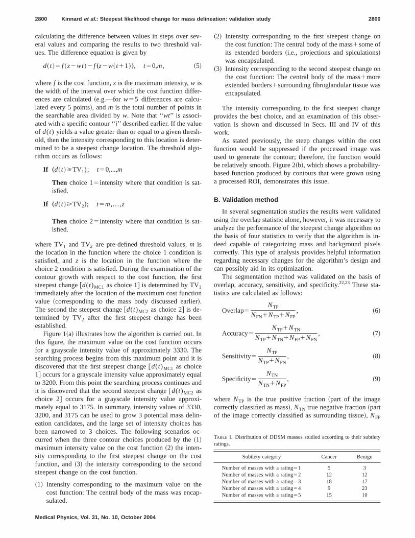
calculating the difference between values in steps over sev-eral values and comparing the results to two threshold val-ues. The difference equation is given by

d� t �� f �z�wt �� f „z�w� t�1 �…, t�0,m , �5�

where f is the cost function, z is the maximum intensity, w isthe width of the interval over which the cost function differ-ences are calculated �e.g.—for w�5 differences are calcu-lated every 5 points�, and m is the total number of points inthe searchable area divided by w. Note that ‘‘wt’’ is associ-ated with a specific contour ‘‘i’’ described earlier. If the valueof d(t) yields a value greater than or equal to a given thresh-old, then the intensity corresponding to this location is deter-mined to be a steepest change location. The threshold algo-rithm occurs as follows:

If „d� t ��TV1); t�0,...,m

Then choice 1�intensity where that condition is sat-isfied.

If „d� t ��TV2…; t�m , . . . ,z

Then choice 2�intensity where that condition is sat-isfied.

where TV1 and TV2 are pre-defined threshold values, m isthe location in the function where the choice 1 condition issatisfied, and z is the location in the function where thechoice 2 condition is satisfied. During the examination of thecontour growth with respect to the cost function, the firststeepest change �d(t)MC1 as choice 1� is determined by TV1

immediately after the location of the maximum cost functionvalue �corresponding to the mass body discussed earlier�.The second the steepest change �d(t)MC2 as choice 2� is de-termined by TV2 after the first steepest change has beenestablished.

Figure 1�a� illustrates how the algorithm is carried out. Inthis figure, the maximum value on the cost function occursfor a grayscale intensity value of approximately 3330. Thesearching process begins from this maximum point and it isdiscovered that the first steepest change �d(t)MC1 as choice1� occurs for a grayscale intensity value approximately equalto 3200. From this point the searching process continues andit is discovered that the second steepest change �d(t)MC2 aschoice 2� occurs for a grayscale intensity value approxi-mately equal to 3175. In summary, intensity values of 3330,3200, and 3175 can be used to grow 3 potential mass delin-eation candidates, and the large set of intensity choices hasbeen narrowed to 3 choices. The following scenarios oc-curred when the three contour choices produced by the �1�maximum intensity value on the cost function �2� the inten-sity corresponding to the first steepest change on the costfunction, and �3� the intensity corresponding to the secondsteepest change on the cost function.

�1� Intensity corresponding to the maximum value on thecost function: The central body of the mass was encap-sulated.

�2� Intensity corresponding to the first steepest change onthe cost function: The central body of the mass�some ofits extended borders �i.e., projections and spiculations�was encapsulated.

�3� Intensity corresponding to the second steepest change onthe cost function: The central body of the mass�moreextended borders�surrounding fibroglandular tissue wasencapsulated.

The intensity corresponding to the first steepest changeprovides the best choice, and an examination of this obser-vation is shown and discussed in Secs. III and IV of thiswork.

As stated previously, the steep changes within the costfunction would be suppressed if the processed image wasused to generate the contour; therefore, the function wouldbe relatively smooth. Figure 2�b�, which shows a probability-based function produced by contours that were grown usinga processed ROI, demonstrates this issue.

B. Validation method

In several segmentation studies the results were validatedusing the overlap statistic alone, however, it was necessary toanalyze the performance of the steepest change algorithm onthe basis of four statistics to verify that the algorithm is in-deed capable of categorizing mass and background pixelscorrectly. This type of analysis provides helpful informationregarding necessary changes for the algorithm’s design andcan possibly aid in its optimization.

The segmentation method was validated on the basis ofoverlap, accuracy, sensitivity, and specificity.22,23 These sta-tistics are calculated as follows:

Overlap�NTP

NFN�NTP�NFP, �6�

Accuracy�NTP�NTN

NTP�NTN�NFP�NFN, �7�

Sensitivity�NTP

NTP�NFN, �8�

Specificity�NTN

NTN�NFP, �9�

where NTP is the true positive fraction �part of the imagecorrectly classified as mass�, NTN true negative fraction �partof the image correctly classified as surrounding tissue�, NFP

TABLE I. Distribution of DDSM masses studied according to their subtletyratings.

Subtlety category Cancer Benign

Number of masses with a rating�1 5 3Number of masses with a rating�2 12 12Number of masses with a rating�3 18 17Number of masses with a rating�4 9 23Number of masses with a rating�5 15 10

2800 Kinnard et al.: Steepest likelihood change for mass delineation: validation study 2800

Medical Physics, Vol. 31, No. 10, October 2004

is the false positive fraction �part of the image incorrectlyclassified as mass�, and NFN is the false negative fraction�part of the image incorrectly classified as surrounding tis-sue�. This method requires a gold standard, or, a contour towhich the segmentation results can be compared. The goldstandards for the experiments performed in this work weremass contours, which have been traced by expert radiolo-gists.

The experiments produced contours for the intensity val-ues resulting from three locations within the cost functions:�1� The intensity of the maximum value within the cost func-tion; �2� the intensity for which the cost function experiencesits first steepest change; and �3� the intensity for which thecost function experiences its second steepest change. It hasbeen observed that the intensity for which the cost functionexperiences its first steepest change produces the contourtrace that is most highly correlated with the gold standardtraces, regarding overlap and accuracy. In cases for whichbetter results occur at the second steepest change location,there is no significant difference between these results andthe results calculated for the first steepest change location.Second, it has been observed that the results are more closelycorrelated with one expert than with the second expert. Thesehypotheses were tested using the one-way Analysis of Vari-

ance �ANOVA� test.24,25 In this study, three significance lev-els �i.e., p�0.001, p�0.01, and p�0.05) were used to cat-egorize the ANOVA results as described in the next section.

III. EXPERIMENTS AND RESULTS

The following sections describe the database and experi-ments, and provide segmentation results and ANOVA testresults.

A. Database

For this study, a total of 124 masses were chosen from theUniversity of South Florida’s Digital Database for ScreeningMammography �DDSM�.26 The DDSM films were digitizedat 43.5 or 50 �m’s using either the Howtek or Lumisys digi-tizers, respectively. The DDSM cases have been ranked byexpert radiologists on a scale from 1 to 5, where 1 representsthe most subtle masses and 5 represents the most obviousmasses. Table I lists the distribution of the masses studiedaccording to their subtlety ratings. The images were of vary-ing contrasts and the masses were of varying sizes.

FIG. 3. �a� Segmentation results for a malignant mass with spiculated mar-gins (subtlety�2) �b� the corresponding cost function.

FIG. 4. �a� Segmentation results for a malignant mass with ill-defined mar-gins (subtlety�3); �b� the corresponding cost function.

2801 Kinnard et al.: Steepest likelihood change for mass delineation: validation study 2801

Medical Physics, Vol. 31, No. 10, October 2004

The first set of expert traces was provided by an attendingphysician at Georgetown University Medical Center�GUMC�, and is hereafter referred to as the Expert A traces.The second set of expert traces was provided by the DDSM,and is hereafter referred to as the Expert B traces.

B. Experiments

As mentioned previously, the term ‘‘steepest change’’ isvery subjective. Therefore, a set of thresholds needed to beset in an effort to define a particular location within the costfunction as a ‘‘steepest change location.’’ For this studythe following thresholds were experimentally chosen:TV1�1800, TV2�1300, where TV1 equals the threshold forsteepest change location 1 for the cost function, and TV2

equals the threshold for steepest change location 2 for thecost function. A number of experiments were performed inan effort to prove that �1� the intensity for which the costfunction experiences the first steepest change location pro-duces the contour trace, which is most highly correlated withthe gold standard traces with regard to overlap and accuracy.In cases for which the second steepest change locationachieves better results, there are no significant differencesbetween the values obtained from the first steepest change

location and the second steepest change location. The experi-ments linked with these hypotheses comprise the studies fora single observer. We have also set out to prove that �2� ourresults are more closely correlated with one expert than withthe second expert. The experiments linked with this hypoth-esis comprise the studies between two observers. First seg-mentation results for two malignant cases are presented, fol-lowed by segmentation results for two benign cases. Second,the ANOVA results for a set of hypotheses are presented. Thecontours produced by the maximum value as well as by thesteepest change locations within the cost functions are la-beled as follows: �1� group 1: The intensity for which a valuewithin the cost function is maximum; �2� group 2: The inten-sity for which the cost function experiences its first steepestchange; �3� group 3: The intensity for which the cost func-tion experiences its second steepest change.

C. Results

Figures 3–6 display the results for two malignant casesaccompanied by their cost functions as well as results for twobe--nign cases accompanied by their cost functions. TheANOVA results appear in a set of tables �Secs. II–IV�, whereeach table lists the hypothesis tested along with p-values andtheir corresponding categorizations. The p-values are catego-

FIG. 5. �a� Segmentation results for a benign mass with ill-defined margins(subtlety�3); �b� the corresponding cost function.

FIG. 6. �a� Segmentation results for a benign mass with circumscribed mar-gins (subtlety�4); �b� the corresponding cost function.

2802 Kinnard et al.: Steepest likelihood change for mass delineation: validation study 2802

Medical Physics, Vol. 31, No. 10, October 2004

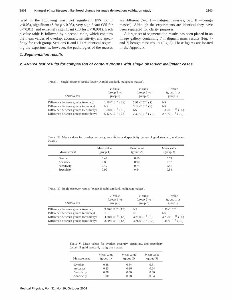
rized in the following way: not significant �NS for p�0.05), significant �S for p�0.05), very significant �VS forp�0.01), and extremely significant �ES for p�0.001). Eachp-value table is followed by a second table, which containsthe mean values of overlap, accuracy, sensitivity, and speci-ficity for each group. Sections II and III are identical regard-ing the experiments, however, the pathologies of the masses

are different �Sec. II—malignant masses, Sec. III—benignmasses�. Although the experiments are identical they havebeen separated for clarity purposes.

A larger set of segmentation results has been placed in animage gallery containing 7 malignant mass results �Fig. 7�and 7� benign mass results �Fig. 8�. These figures are locatedin the Appendix.

1. Segmentation results

2. ANOVA test results for comparison of contour groups with single observer: Malignant cases

TABLE II. Single observer results �expert A gold standard, malignant masses�.

ANOVA test

P-value�group 1 vs

group 2�

P-value�group 2 vs

group 3�

P-value�group 1 vs

group 3�

Difference between groups �overlap� 1.78�10�4 (ES) 2.91�10�2 (S) NSDifference between groups �accuracy� NS 3.14�10�2 (S) NSDifference between groups �sensitivity� 1.88�10�9 (ES) NS 1.85�10�13 (ES)Difference between groups �specificity� 5.12�10�4 (ES) 2.40�10�3 (VS) 2.71�10�9 (ES)

TABLE III. Mean values for overlap, accuracy, sensitivity, and specificity �expert A gold standard, malignantmasses�.

MeasurementMean value�group 1�

Mean value�group 2�

Mean value�group 3�

Overlap 0.47 0.60 0.53Accuracy 0.88 0.90 0.87Sensitivity 0.49 0.75 0.81Specificity 0.99 0.94 0.88

TABLE IV. Single observer results �expert B gold standard, malignant masses�.

ANOVA test

P-value�group 1 vs

group 2�

P-value�group 2 vs

group 3�

P-value�group 1 vs

group 3�

Difference between groups �overlap� 3.96�10�6 (ES) NS 1.58�10�4

Difference between groups �accuracy� NS NS NSDifference between groups �sensitivity� 4.88�10�8 (ES) 4.31�10�2 (S) 4.25�10�12 (ES)Difference between groups �specificity� 2.70�10�4 (ES) 4.36�10�4 (ES) 1.44�10�7 (ES)

TABLE V. Mean values for overlap, accuracy, sensitivity, and specificity�expert B gold standard, malignant masses�.

MeasurementMean value�group 1�

Mean value�group 2�

Mean value�group 3�

Overlap 0.38 0.54 0.51Accuracy 0.83 0.86 0.84Sensitivity 0.38 0.56 0.60Specificity 1.00 0.98 0.94

2803 Kinnard et al.: Steepest likelihood change for mass delineation: validation study 2803

Medical Physics, Vol. 31, No. 10, October 2004

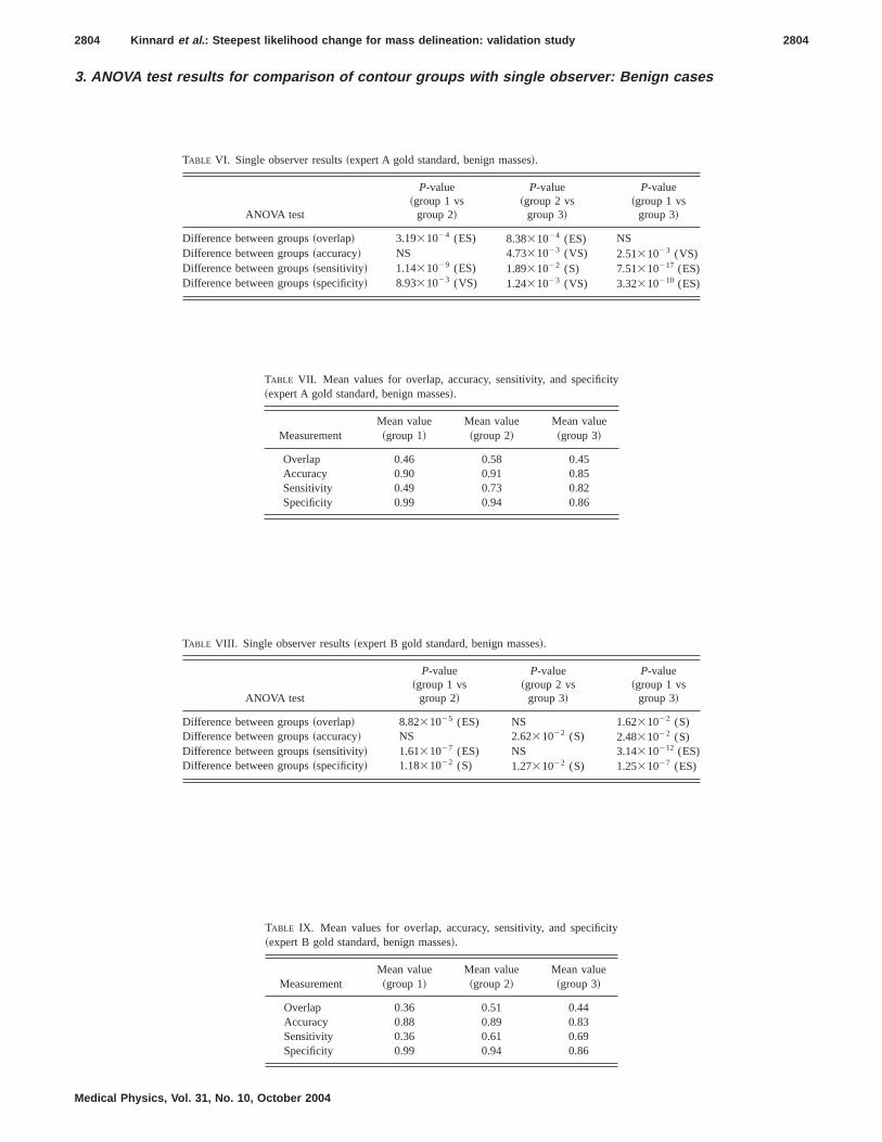
3. ANOVA test results for comparison of contour groups with single observer: Benign cases

TABLE VI. Single observer results �expert A gold standard, benign masses�.

ANOVA test

P-value�group 1 vs

group 2�

P-value�group 2 vs

group 3�

P-value�group 1 vs

group 3�

Difference between groups �overlap� 3.19�10�4 (ES) 8.38�10�4 (ES) NSDifference between groups �accuracy� NS 4.73�10�3 (VS) 2.51�10�3 (VS)Difference between groups �sensitivity� 1.14�10�9 (ES) 1.89�10�2 (S) 7.51�10�17 (ES)Difference between groups �specificity� 8.93�10�3 (VS) 1.24�10�3 (VS) 3.32�10�10 (ES)

TABLE VII. Mean values for overlap, accuracy, sensitivity, and specificity�expert A gold standard, benign masses�.

MeasurementMean value�group 1�

Mean value�group 2�

Mean value�group 3�

Overlap 0.46 0.58 0.45Accuracy 0.90 0.91 0.85Sensitivity 0.49 0.73 0.82Specificity 0.99 0.94 0.86

TABLE VIII. Single observer results �expert B gold standard, benign masses�.

ANOVA test

P-value�group 1 vs

group 2�

P-value�group 2 vs

group 3�

P-value�group 1 vs

group 3�

Difference between groups �overlap� 8.82�10�5 (ES) NS 1.62�10�2 (S)Difference between groups �accuracy� NS 2.62�10�2 (S) 2.48�10�2 (S)Difference between groups �sensitivity� 1.61�10�7 (ES) NS 3.14�10�12 (ES)Difference between groups �specificity� 1.18�10�2 (S) 1.27�10�2 (S) 1.25�10�7 (ES)

TABLE IX. Mean values for overlap, accuracy, sensitivity, and specificity�expert B gold standard, benign masses�.

MeasurementMean value�group 1�

Mean value�group 2�

Mean value�group 3�

Overlap 0.36 0.51 0.44Accuracy 0.88 0.89 0.83Sensitivity 0.36 0.61 0.69Specificity 0.99 0.94 0.86

2804 Kinnard et al.: Steepest likelihood change for mass delineation: validation study 2804

Medical Physics, Vol. 31, No. 10, October 2004

4. ANOVA test results for comparison of contour groups between two observers

TABLE X. Two observer results: expert A vs expert B, malignant masses.

ANOVA test

P-value�group 1 vs

group 2�

P-value�group 2 vs

group 3�

P-value�group 1 vs

group 3�

Expert A vs expert B �overlap� 3.12�10�3 (VS) 3.32�10�2 (S) NSExpert A vs expert B �accuracy� 1.20�10�2 (S) 4.46�10�2 (S) NSExpert A vs expert B �sensitivity� 9.43�10�4 (ES) 3.38�10�4 (ES) 3.67�10�4 (ES)Expert A vs expert B �specificity� NS NS NS

TABLE XI. Mean values for overlap, accuracy, sensitivity, and specificity �expert A vs expert B, malignant masses�.

Measurement

Meanvalue,

expert A�group 1�

Meanvalue,

expert B�group 1�

Meanvalue,

expert A�group 2�

Meanvalue,

expert B�group 2�

Meanvalue,

expert A�group 3�

Meanvalue,

expert B�group 3�

Overlap 0.49 0.38 0.62 0.55 0.55 0.51Accuracy 0.89 0.83 0.91 0.87 0.87 0.84Sensitivity 0.52 0.38 0.75 0.60 0.82 0.68Specificity 0.99 1.00 0.95 0.97 0.89 0.91

TABLE XII. Two observer results: expert A vs expert B, benign masses.

ANOVA test

P-value�group 1 vs

group 2�

P-value�group 2 vs

group 3�

P-value�group 1 vs

group 3�

Expert A vs expert B �overlap� NS NS NSExpert A vs expert B �accuracy� NS NS NSExpert A vs expert B �sensitivity� 3.56�10�2 (S) 4.90�10�2 (S) 2.03�10�2 (S)Expert A vs expert B �specificity� NS NS NS

TABLE XIII. Mean values for overlap, accuracy, sensitivity, and specificity: expert A vs expert B, benign masses.

Measurement

Meanvalue,

expert A�group 1�

Meanvalue,

expert B�group 1�

Meanvalue,

expert A�group 2�

Meanvalue,

expert B�group 2�

Meanvalue,

expert A�group 3�

Meanvalue,

expert B�group 3�

Overlap 0.42 0.35 0.57 0.50 0.48 0.44Accuracy 0.90 0.88 0.91 0.89 0.85 0.83Sensitivity 0.44 0.36 0.71 0.61 0.79 0.69Specificity 0.99 0.99 0.94 0.94 0.86 0.86

2805 Kinnard et al.: Steepest likelihood change for mass delineation: validation study 2805

Medical Physics, Vol. 31, No. 10, October 2004

IV. DISCUSSION

A. Segmentation results

The ROI’s shown in Figs. 3 and 4 demonstrate that theintensity produced by the maximum value is capable of ac-curately delineating the mass body contour, and in somecases this intensity corresponding to the maximum valueproduces a contour, which falls inside the mass body contour.This situation can be problematic because low segmentationsensitivities can produce large errors during the feature cal-culation and classification phases of CADx . Of the threeavailable segmentation choices for each mass, it appears thatthe first steepest change location produces the contours withthe strongest correlation in comparison to both gold stan-dards. These contours appear to cover both the mass bodycontour as well as the extended borders. In some instancesthe region grows into some areas that are not declared asmass areas by the gold standards—we call this flooding—and fails to grow into other areas that have been declared asmass areas. Finally, the second steepest change location pro-duces contours that also cover both the mass body contour aswell as the extended borders, and, these contours tend to alsoinclude surrounding fibroglandular tissue; hence, the flood-ing phenomenon is a common occurrence. In the casesshown, it is clear that steepest change location 1 produces thebest contours, in comparison to the gold standards, however,the ANOVA test results allow us to make such a claim. Thefollowing discussion is divided into five sections: single ob-server malignant results, single observer benign results, andtwo observer results �malignant and benign�, algorithm per-formance, and an additional discussion on methods.

B. Malignant cases with single observer

For both the expert A and expert B gold standards, TablesII–V show a statistically significant difference betweengroups 1 and 2 on the basis of overlap and sensitivity, wherethe mean values of group 2 were higher than the mean valuesof group 1 for these statistics. These results are expectedbecause as shown in the figures, the group 2 contours con-sistently covered more of the mass area �and correctly cov-ered this mass area� as compared to the group 1 contours,according to both experts. There was a statistically signifi-cant difference in sensitivity between group 1 and group 3,where the mean of group 3 was higher than the mean ofgroup 1. This difference is an expected result because out ofall the groups, group 3 contours consistently covered themost mass area. For the expert B gold standard there was astatistically significant difference in overlap between group 1and group 3, where the mean of group 3 was higher than themean of group 1. This difference is also an expected resultbecause, out of all the groups, the group 3 contours coveredthe most mass area correctly.

C. Benign cases with single observer

For the expert A traces there were statistically significantdifferences between the group 2 and group 3 traces on the

basis of overlap, accuracy, and sensitivity, where the group 2mean values for overlap and accuracy were higher than thoseof group 3 �see Tables VI–IX�. This difference is an ex-pected result because it is likely that many of the group 3contours contained flooded areas, which cause both of thesevalues to be lower than those values of contours withoutflooded areas. The overlap and sensitivity values for group 2were significantly higher than those of group 1. This differ-ence is also an expected result because the group 2 contoursnot only covered more mass area but also covered this areacorrectly. Finally, the group 3 accuracy and sensitivity valueswere significantly higher than those for group 1. Again thisdifference is an expected result because the group 3 contoursnot only covered more mass area but they also covered thisarea correctly.

For the expert B gold standard there were statisticallysignificant differences between the group 2 and group 3traces on the basis of accuracy and sensitivity, where thegroup 2 mean values for overlap and accuracy were higherthan those of group 3. This difference is an expected resultbecause it is likely that many of the group 3 contours con-tained flooded areas, which cause both of these values to belower than contours without flooded areas. There were sta-tistically significant differences between group 1 and group 2on the basis of overlap and sensitivity, where the mean val-ues for group 2 were higher than the mean values for group1. This is an expected result because the group 2 contours notonly covered more mass area but they also covered this areacorrectly. There were statistically significant differences be-tween group 3 and group 1 on the basis of overlap and sen-sitivity, where the mean values for group 3 were higher thanthose of group 1. Again this difference is an expected resultbecause the group 3 contours not only covered more massarea but they covered this area correctly.

In nearly all cases for the single observer studies, it wasexpected that the specificity values for group 1 would alwaysbe higher than those for groups 2 and 3 because this contouralways covered the smallest mass area; consequently itsbackground was always highly correlated with the back-ground areas dictated by the gold standards. Moreover, insome cases the group 2 and group 3 contours grew into areasthat were not regarded as mass, but rather were regarded asbackground; therefore, their specificity values had a lowercorrelation with the gold standard as compared to the group1 contours.

D. Malignant and benign cases with two observers

For the two observer studies, comparisons were made be-tween experts A and B on a group-by-group basis in an effortto prove that there were significant differences between thetwo radiologists on the basis of overlap, accuracy, sensitivity,and specificity �see Tables X–XIII�. For the malignantmasses, there were statistically significant differences be-tween the two experts on the basis of overlap, accuracy, andsensitivity. There was a statistically significant difference be-tween the two experts for group 3 on the basis of sensitivity.For the benign masses, there were statistically significant dif-ferences between the two experts for all three groups on the

2806 Kinnard et al.: Steepest likelihood change for mass delineation: validation study 2806

Medical Physics, Vol. 31, No. 10, October 2004

basis of sensitivity. For all cases, expert A’s values were con-sistently higher than those of expert B. These statisticallysignificant differences between the experts were expecteddue to their differences in opinion. The fact that expert A’smean values were higher than those for expert B, however,does not warrant the conclusion that expert A is a more reli-able expert; however, it does warrant the conclusion thatthere is stronger agreement between the computer’s resultsand expert A’s traces. Furthermore, there were less statisti-cally significant differences for the benign cases than for themalignant cases. This result is expected because, in general,benign masses have better defined borders, and thus the twoexperts were more likely to agree.

E. Algorithm performance

Apparently the chosen thresholds produce first steepestchange location intensities that generate contours closelycorrelated with the expert traces. In some instances the sec-ond steepest change location is extremely far from the firststeepest change location, which implies that the function inquestion increases very slowly; moreover, many of the sec-ond steepest change location intensities produce contourswith flooded areas. For the majority of the cases in which thesecond steepest change location contour achieves a highersensitivity value, but not a significantly higher sensitivityvalue, we can still choose the first steepest change locationcontour because the difference between the two contours islikely to be negligible.

In analyzing the probability-based cost functions, wefound that those functions with very steep changes are typi-cally associated with masses that have well-defined borderswhile those functions that increase slowly are associatedwith masses that have ill-defined borders. This phenomenonmay make it necessary to develop an adaptive threshold pro-cess for the steepest change evaluation such that the func-tions are grouped into various categories �e.g., smooth versussteep�, because a threshold value that is optimal for a steepfunction may not be optimal for a smooth function.

F. Additional discussion on methods used

In this study the steepest descent method appears to havethe advantage of locating ill-defined margins as well as ex-tensions such as malignant spiculations and projections formammographic masses. If solely the human eye is used, itcan be difficult to separate the mass from the surroundingfibroglandular tissue. Therefore, this method has the poten-tial to complement the process of reading mammographicfilms. One of the downfalls of the method is its dependenceupon the assumption that masses are generally light in color.This assumption impedes the region growing process be-cause masses that contain darker areas and are surrounded onone or more sides by bright tissue can cause contours toflood into areas that are not actual mass tissue. Typically, thissituation occurs for the mass located on the border of thebreast region on a mammogram.

All of the segmentation methods surveyed in the introduc-tion of this paper are excellent solutions for the problems

their authors set out to solve, however, in some cases it isdifficult to make comparisons between different methodswithout the availability of a set of several visual results. Insome studies, the focus was either to detect masses or todistinguish malignant from benign masses. Thus, the valida-tion process did not take the form of a comparison withexpert radiologist manual traces; but rather, features werecalculated on the potential mass candidates and they werelater classified as being mass tissue or normal tissue.10–13

The purpose of Li’s study14 was to distinguish between nor-mal and abnormal tissue; thus the authors did not provideany statistics such as overlap or accuracy. Nevertheless, thestudy contains a figure of 60 masses that contain both com-puter and radiologist annotations to give the reader an idea ofthe computer algorithm’s performance. Te Brake and Karsse-meijer’s study9 used the overlap statistic to test the efficacyof their method. They indicated that the central mass areawas delineated by the radiologist and their computer resultswere compared to these annotations. The Kupinski and Gigerstudy16 also used the overlap statistic to test the efficacy oftheir method and set a threshold for which the mass wasconsidered to be successfully segmented. For example,masses whose overlap values are greater than 0.7 imply thatthere was successful segmentation.

The technical method presented herein shows that the re-sults obtained from the maximization of the composed prob-ability density function �i.e., the cost function� are equivalentto those obtained from previous methods presented by pre-vious investigators. However, the steepest change of thecomposed probability density function is the closest to radi-ologists’ determinations.

V. CONCLUSION

We have shown that our fully automatic boundary detec-tion method for malignant and benign masses can effectivelydelineate these masses using intensities, that correspond tothe first steepest change location within their cost functions.Additionally, the method appears to be more highly corre-lated with one set of expert traces than with a second set ofexpert traces, regarding the accuracy and overlap statistics.This result shows that inter-observer variability can be animportant factor in segmentation algorithm design, and it hasmotivated us to seek the opinions of more expert radiologiststo test the robustness of our algorithm. The second steepestchange location intensity will always yield contours withhigher sensitivity values, however, it behooves us to choosethe first steepest change location intensity because it avoidsthe risk of choosing contours that contain substantial flood-ing. In future work, a worthwhile study would run the ex-periments for different threshold values in an effort to dis-cover the possibility of deriving an optimal thresholdprocedure. We believe that such a procedure would improvethe method of choosing optimal contours.

2807 Kinnard et al.: Steepest likelihood change for mass delineation: validation study 2807

Medical Physics, Vol. 31, No. 10, October 2004

ACKNOWLEDGMENTS

This work was supported by U.S. Army Grant Nos.DAMD17-03-1-0314, DAMD17-01-1-0267, and DAMD

17-00-1-0291, and NIH Grant No. RCMI/NCRR/NIH2G12RR00348. The authors would also like to thank thereferees for their constructive comments and recommenda-tions.

APPENDIX A—GALLERY OF SEGMENTATION RESULTS

FIG. 7. Segmentation results for a setof malignant masses.

2808 Kinnard et al.: Steepest likelihood change for mass delineation: validation study 2808

Medical Physics, Vol. 31, No. 10, October 2004

a�Author to whom correspondence should be addressed. Dr. Shih-Chung B.Lo, ISIS Center, Department of Radiology, Georgetown University, Box571479, Washington, DC 20057-1479. Electronic mail:lo@isis.imac.georgetown.edu

1 J. V. Lacey, Jr., S. S. Devesa, and L. A. Brinton, ‘‘Recent trends in breastcancer incidence and mortality,’’ Environ. Mol. Mutagen. 39, 82–88�2002�.

2 J. E. Meyer, D. B. Kopans, P. C. Stomper, and K. K. Lindfors, ‘‘Occultbreast abnormalities: percutaneous preoperative needle localization,’’ Ra-diology 150, 335–337 �1984�.

3 A. L. Rosenberg, G. F. Schwartz, S. A. Feig, and A. S. Patchefsky,‘‘Clinically occult breast lesions: localization and significance,’’ Radiol-ogy 162, 167–170 �1987�.

4 B. C. Yankaskas, M. H. Knelson, M. L. Abernethy, J. T. Cuttino, and R.

L. Clark, ‘‘Needle localization biopsy of occult lesions of the breast,’’Radiology 23, 729–733 �1988�.

5 J. A. Harvey, L. L. Fajardo, and C. A. Innis, ‘‘Previous mammograms inpatients with impalpable breast carcinoma: retrospective vs. blinded in-terpretation,’’ Am. J. Roentgenol., Radium Ther. Nucl. Med. 161, 1167–1172 �1993�.

6 J. E. Martin, M. Moskowitz, and J. R. Milbrath, ‘‘Breast cancer missedby mammography,’’ Am. J. Roentgenol., Radium Ther. Nucl. Med. 132,737–739 �1979�.

7 J. R. Harris, M. E. Lippman, M. Morrow, and S. Hellman, Diseases of theBreast �Lippincott-Raven Publishers, Philadelphia, 1996�, pp. 80–81.

8 J. E. Martin, Atlas of Mammography: Histologic and MammographicCorrelations, 2nd ed. �Williams and Wilkins, Baltimore, 1988�, p. 87.

9 G. M. te Brake and N. Karssemeijer, ‘‘Segmentation of suspicious den-

FIG. 8. Segmentation results for a setof benign masses.

2809 Kinnard et al.: Steepest likelihood change for mass delineation: validation study 2809

Medical Physics, Vol. 31, No. 10, October 2004

sities in digital mammograms,’’ Med. Phys. 28, 259–266 �2001�.10 L. Li, Y. Zheng, L. Zhang, and R. Clark, ‘‘False-positive reduction in

CAD mass detection using a competitive classification strategy,’’ Med.Phys. 28, 250–258 �2001�.

11 N. Petrick, H.-P. Chan, B. Sahiner, and D. Wei, ‘‘An adaptive density-weighted contrast enhancement filter for mammographic breast mass de-tection,’’ IEEE Trans. Med. Imaging 15, 59–67 �1996�.

12 S. Pohlman, K. A. Powell, N. A. Obuchowski, W. A. Chilcote, and S.Grundfest-Broniatowski, ‘‘Quantitative classification of breast tumors indigitized mammograms,’’ Med. Phys. 23, 1337–1345 �1996�.

13 A. J. Mendez, P. G. Tahoces, M. J. Lado, M. Souto, and J. J. Vidal,‘‘Computer-aided diagnosis: Automatic detection of malignant masses indigitized mammograms,’’ Med. Phys. 25, 957–964 �1998�.

14 H. Li, Y. Wang, K. J. R. Liu, S.-C. B. Lo, and M. T. Freedman, ‘‘Com-puterized radiographic mass detection—part I: lesion site selection bymorphological enhancement and contextual segmentation,’’ IEEE Trans.Med. Imaging 20, 289–301 �2001�.

15 M. L. Comer, S. Liu, and E. J. Delp, ‘‘Statistical segmentation of mam-mograms,’’ Digital Mammography ’96: proceedings of the 3rd interna-tional workshop on digital mammography, Chicago, IL, pp. 475–478,9–12 June 1996.

16 M. A. Kupinski and M. L. Giger, ‘‘Automated seeded lesion segmenta-tion on digital mammograms,’’ IEEE Trans. Med. Imaging 17, 510–517�1998�.

17 S.-C. B. Lo, H. Li, Y. Wang, L. Kinnard, and M. T. Freedman, ‘‘A mul-tiple circular path convolution neural network system for detection ofmammographic masses,’’ IEEE Trans. Med. Imaging 21, 150–158�2002�.

18 W. E. Polakowski, D. A. Cournoyer, S. K. Rogers, M. P. DeSimio, D. W.Ruck, J. W. Hoffmeister, and R. A. Raines, ‘‘Computer-aided breast can-cer detection and diagnosis of masses using difference of Gaussians andderivative-based feature saliency,’’ IEEE Trans. Med. Imaging 16, 811–819 �1997�.

19 B. Sahiner, H.-P. Chan, N. Petrick, M. A. Helvie, and L. M. Hadjiiski,‘‘Improvement of mammographic mass characterization using spiculationmeasures and morphological features,’’ Med. Phys. 28, 1455–1465�2001�.

20 R. M. Rangayyan, N. M. El-Faramawy, J. E. Leo Desautels, and O. A.Alim, ‘‘Measures of acutance and shape for classification of breast tu-mors,’’ IEEE Trans. Med. Imaging 16, 799–810 �1997�.

21 B. Sahiner, H.-P. Chan, D. Wei, N. Petrick, M. A. Helvie, D. D. Adler,and M. M. Goodsit, ‘‘Image feature selection by a genetic algorithm:Application to classification of mass and normal breast tissue,’’ Med.Phys. 23, 1671–1684 �1996�.

22 J. Suckling, D. R. Dance, E. Moskovic, D. J. Lewis, and S. G. Blacker,‘‘Segmentation of mammograms using multiple linked self-organizingneural networks,’’ Med. Phys. 22, 145–152 �1995�.

23 B. Van Ginneken, ‘‘Automatic segmentation of lung fields in chest radio-graphs,’’ Med. Phys. 27, 2445–2455 �2000�.

24 D. Downing and J. Clark, Statistics the Easy Way, 2nd ed. �Barron’sEducational Series, Hauppauge, 1989�, pp. 184–206.

25 W. Hopkins, A New View of Statistics: P Values and Statistical Signifi-cance; available online at www.sportsci.org/resource/stats/pvalues.html.

26 M. Heath et al., ‘‘Current status of the digital database for screeningmammography,’’ Digital Mammography �Kluwer Academic, New York,1998�, pp. 457–460.

2810 Kinnard et al.: Steepest likelihood change for mass delineation: validation study 2810

Medical Physics, Vol. 31, No. 10, October 2004

A Tumor-Targeted Nanodelivery System to Improve Early MRIDetection of Cancer

Kathleen F. Pirollo1, John Dagata2, Paul Wang3, Matthew Freedman1, Andras Vladar2, Stanley Fricke1,

Lilia Ileva1, Qi Zhou1, and Esther H. Chang1

1Georgetown University Medical Center, 2National Institute of Standards and Technology, and 3Howard University

AbstractThe development of improvements in magnetic resonance

imaging (MRI) that would enhance sensitivity, leading to

earlier detection of cancer and visualization of metastatic

disease, is an area of intense exploration. We have devised a

tumor-targeting, liposomal nanodelivery platform for use in

gene medicine. This systemically administered nanocomplex

has been shown to specifically and efficiently deliver both

genes and oligonucleotides to primary and metastatic tumor

cells, resulting in significant tumor growth inhibition and even

tumor regression. Here we examine the effect on MRI of

incorporating conventional MRI contrast agent Magnevist1

into our anti-transferrin receptor single-chain antibody

(TfRscFv) liposomal complex. Both in vitro and in an in vivo

orthotopic mouse model of pancreatic cancer, we show

increased resolution and image intensity with the complexed

Magnevist1. Using advanced microscopy techniques (scanning

electron microscopy and scanning probe microscopy), we also

established that the Magnevist1 is in fact encapsulated by the

liposome in the complex and that the complex still retains its

nanodimensional size. These results demonstrate that this

TfRscFv–liposome–Magnevist1 nanocomplex has the potential

to become a useful tool in early cancer detection. Mol Imaging

(2006) 5, 41–52.

Keywords: Nanocomplex, tumor targeting, Magnevist1, MRI, early detection.

Introduction

The ability to detect cancer, both primary and metastatic

disease, at an early stage would be a major step toward

the goal of ending the pain and suffering from the

disease. The development of tumor-targeted delivery

systems for gene therapy has opened the potential for

delivery of imaging agents more effectively than is

currently achievable. Magnetic resonance imaging

(MRI) can acquire 3-D anatomical images of organs.

Coupling these with paramagnetic images results in

the accurate localization of tumors as well as longitudi-

nal and quantitative monitoring of tumor growth and

angiogenesis [1,2].

One of the most common paramagnetic imaging

agents used in cancer diagnostics is Magnevist1 (gado-

pentetate dimeglumine). Gadolinium is a rare earth

element. It shows paramagnetic properties because its

ion (Gd2+) has seven unpaired electrons. The contrast

enhancement observed in MRI scans is due to the strong

effect of Gd2+ primarily on the hydrogen-proton spin–

lattice relaxation time (T1). Whereas free gadolinium is

highly toxic and thus unsuitable for clinical use, chela-

tion with diethylenetriamine pentacetic acid generates a

well-tolerated, stable, strongly paramagnetic complex.

This metal chelate is metabolically inert. However,

after intravenous (iv) injection of gadopentetate dime-

glumine, the meglumine ion dissociates from the hydro-

phobic gadopentetate, which is distributed only in the

extracellular water. It cannot cross an intact blood–brain

barrier and therefore does not accumulate in normal

brain tissue, cysts, postoperative scars, etc, and it is

rapidly excreted in the urine. It has a mean half-life of

about 1.6 hr. Approximately 80% of the dose is excreted

in the urine within 6 hr.

A systemically administered tumor-targeting delivery

system has been developed in our laboratory for use in

gene medicine [3–8]. This nanosized complex is com-

posed of a cationic liposome encapsulating the nucleic

acid payload, which can be either genes [3–6] or

oligonucleotides [7,8]. Decorating the surface of the

liposome is a targeting molecule that can be a ligand,

such as folate or transferrin, or an antibody or an

antibody fragment directed against a cell surface recep-

tor. The presence of the ligand/antibody on the lipo-

some facilitates the entry of the complex into the cells

through binding of the targeting molecule by its recep-

tor followed by internalization of the bound complex

via receptor-mediated endocytosis, a highly efficient

D 2006 BC Decker Inc

Abbreviations: Lip, liposome; Mag, Magnevist1 (Gadopentetate Dimeglumine); SEM, scanning

electron microscopy; SPM, scanning probe microscopy; STEM, scanning transmission electron

microscopy; TfRscFv, anti-transferrin receptor single chain antibody; TfRscFv-Lip-Mag, anti-

transferrin receptor single chain antibody-liposome-Magnevist1 complex.

Corresponding author: Esther H. Chang, PhD, Department of Oncology, Lombardi Compre-

hensive Cancer Center, Georgetown University Medical Center, 3970 Reservoir Road, NW, The

Research Building, TRB E420, Washington, DC 20057-1460; e-mail: change@georgetown.edu.

Received 25 February 2005; Received in revised form 8 June 2005; Accepted 17 June 2005.

DOI 10.2310/7290.2006.00005

RESEARCH ARTICLE Molecular Imaging . Vol. 5, No. 1, January 2006, pp. 41– 52 41

internalization pathway [9,10]. This modification of the

liposomes results in their being able to not only se-

lectively deliver their payload to tumor cells, but also

increases the transfection efficacy of the liposome.

Transferrin receptor (TfR) levels are elevated in various

types of cancer including oral, prostate, breast, and pan-

creas [11–16]. Moreover, the TfR recycles during inter-

nalization in rapidly developing cells such as cancer cells

[16], thus contributing to the uptake of these transferrin-

targeted nanocomplexes even in cancer cells where TfR

levels are not elevated. The nanocomplex used in the

studies described here uses an anti-transferrin receptor

single-chain antibody fragment (TfRscFv) as the targeting

moiety [17,18]. TfRscFv contains the complete antibody-

binding site for the epitope of the TfR recognized by the

monoclonal antibody 5E9 [18]. TfRscFv has advantages

over the transferrin molecule itself, or an entire mono-

clonal antibody, in targeting liposomes to cancer cells

with elevated TfR levels: (1) The size of the scFv (28 kDa)

is much smaller than that of the transferrin molecule

(80 kDa) or the parental monoclonal antibody (155 kDa).

The scFv liposome–DNA complex may thus exhibit

better penetration into small capillaries characteristic of

solid tumors. (2) The smaller scFv has a practical advan-

tage related to the scaled-up production necessary for

the clinical trials. (3) The scFv is a recombinant mole-

cule and not a blood product like transferrin and thus

presents no danger of a potential contamination by

blood-borne pathogens. (4) Without the Fc region of the

monoclonal antibody, the issue of non-antigen-specific

binding through Fc receptors is eliminated [19]. Most im-

portantly, we have already shown that such an anti-TfR

single-chain antibody molecule can target an intra-

venously administered cationic liposome–DNA nano-

complex preferentially to tumors [5,6]. Encapsulating

Magnevist1 within such a tumor-targeted nanocomplex

offers potential advantages for enhanced sensitivity, de-

tection of metastases, and diagnosis of cancer.

In this article, using a mouse xenograft model of

human pancreatic cancer, we explore the use of this

nanocomplex for systemic delivery of the imaging agent

Magnevist1 to tumors. In addition, we used scanning

electron microscopy (SEM) and scanning probe micros-

copy (SPM) [20–25] to examine the physical structure

and size of these Magnevist1-carrying nanocomplexes.

Because gadolinium is a high-atomic-number element

and possesses a large magnetic moment, these proper-

ties can be exploited in a variety of ways to enhance

contrast in both SEM and SPM. The findings presented

below demonstrate that our ligand–liposome nanocom-

plex does indeed encapsulate Magnevist1 and that iv

administration of this complex results in enhanced

tumor imaging.

Materials and Methods

Cell Lines

Human lymphoblastic leukemia cell line K562 was

obtained from the Lombardi Comprehensive Cancer

Center Tissue Culture core facility (Washington, DC).

These suspension cells were maintained in RPMI 1640

supplemented with 10% heat-inactivated fetal bovine

serum (FBS) plus 2 mM L-glutamine, and 50 mg/mL

each of penicillin, streptomycin, and neomycin. Human

pancreatic cancer cell line CaPan-1 (obtained from

ATCC, Manassas, VA) was derived from a metastatic

adenocarcinoma of the pancreas. It was maintained in

Iscove’s modified Dulbecco’s medium containing 4 mM

L-glutamine and sodium bicarbonate, supplemented

with 20% non-heat-inactivated FBS, 2 mM L-glutamine,

and 50 mg/mL each of penicillin, streptomycin, and

neomycin. Human prostate cancer cell line DU145

(ATCC) was originally derived from a lesion in the

brain of a patient with widespread metastatic carcinoma

of the prostate. It was maintained in minimum essen-

tial medium with Earle’s salts supplemented with 10%

heat-inactivated FBS plus L-glutamine and antibiotics

as above.

Nanocomplex Formation

Cationic liposome (DOTAP:DOPE) was prepared by

the ethanol injection method as previously described

[6]. When delivering plasmid DNA, the full complex was

formed in a manner identical to that previously de-

scribed [26]. To encapsulate the imaging agent, the

TfRscFv was mixed with the liposome at a specific ratio

(identical to that used with DNA) and incubated at room

temperature for 10 min. Magnevist1 was added to this

solution, mixed, and again incubated at room tempera-

ture for 10 min. When stored at 2–8�C the complex is

stable for at least 8 days, as determined by size measure-

ments using a Malvern Zetasizer 3000H (Malvern, UK).

The average of the cumulants (Z average) measurements

over this time frame is 112.3 ± 4.67 (SE), whereas the

polydispersity (representing the reproducibility of the

values during repeat scans) is 0.445 ± 0.03. For in vitro

transfection, 2 mL of serum-free medium was added to

the complex before transfection. When prepared for

in vivo use, dextrose was added to a final concentration

of 5%. For both in vitro and in vivo complex formation,

the ratio of Magnevist1 to liposome was 1:7 (vol/vol).

42 A Nanodelivery Complex for Early Cancer Detection Pirollo et al.

Molecular Imaging . Vol. 5, No. 1, January 2006

In Vitro Transfection

To transfect suspension cells K562, 15 � 106 cells in a

total volume of 4.0 mL of medium with all supplements

except serum (serum-free medium) were placed into a

100-mm2 tissue-culture dish. Two milliliters of the trans-

fection solution from above, containing varying amounts

of Magnevist1, was added to the cell suspension. The

plate was incubated at 37�C with gentle rocking for

the length of time given in the Results section (up to

90 min), after which the cells were gently pelleted

(600 � g for 7 min) at 4�C in 0.5 mL microcentrifuge

tubes and washed three times with 10 mL of serum free

medium to remove any excess transfection solution and

placed on wet ice until imaged.

In Vivo Tumor Targeting

To assess the tumor-selective targeting of the

TfRscFv–liposome (TfRscFv–Lip) nanocomplex to pri-

mary and metastatic tumors, an orthotopic metastasis

model using human pancreatic cancer cell line CaPan-1

was used. Subcutaneous xenograft tumors of CaPan-1

were induced in female athymic nude mice by injection

of 1 � 107 CaPan-1 cells suspended in Matrigel collagen

basement membrane matrix (BD Biosciences, San Jose,

CA). Approximately 8 weeks later, the tumors were

harvested and a single-cell suspension of the tumor

was prepared. Cells (1.2–1.5 � 107), also suspended in

Matrigel were injected into the surgically exposed pan-

creas of female athymic nude mice as previously de-

scribed [27]. Five weeks post surgery, the complex

carrying the LacZ gene was iv injected 3� over 24 hrs

(at 40 mg DNA per injection). Sixty hours later, the

animals were sacrificed and examined for the presence

of metastases and organs stained for b-galactosidaseexpression using a previously described procedure [3].

Magnetic Resonance Imaging

For in vitro MRI, the cell pellets in microcentrifuge

tubes were positioned at the center of the magnet. The

MRI was performed at Howard University using a 4.7-T

horizontal bore NMR machine (Varian Inc, Palo Alto,

CA). The imaging protocols consist of a multislice T1-

weighted spin–echo imaging sequence and a satura-

tion–recovery sequence. For the T1-weighted imaging

technique, the repetition time (TR) was 1000 msec and

the echo time (TE) was 13 msec. The T1-weighted spin–

echo imaging technique was applied to verify the posi-

tive image enhancement. The saturation–recovery MR

sequence with variable echo times was used for the T1

measurement. The slice thickness of images was 0.5 mm.

The radiofrequency (RF) coil used was a 30-mm single-

loop coil. The RF coil serves as an RF transmitter and

receiver. The RF pulse was a selective 5-msec sinc pulse.

The number of phase-encoding steps was 256. The field

of view was 15 � 15 mm. The image area chosen in the

study was at the center of the RF coil for RF homoge-

neity. The MR images were taken in the cross-section

direction of the microcentrifuge tube. The height of the

cell pellet was 12 mm. The range of the multislice images

covers the whole pellet. The center slice images, which

were not influenced by the image distortion due to the

susceptibility effect from the air–pellet boundary, were

used for the studies. The image intensity was measured

using the Varian Image Browser software. The signal is

taken from a region of interest that is big enough to

cover two thirds of the image from each microcentrifuge

tube. The relative image intensities of the pellets from

these tubes were applied for contrast enhancement

evaluation and the T1 measurements.

For the in vivo studies, mice bearing CaPan-1 ortho-

topic tumors or DU145 subcutaneous xenograft tumors

were used. The CaPan-1 tumors were induced as de-

scribed above. DU145 tumors were induced by the

subcutaneous inoculation of 7 � 106 cells in Matrigel.

These studies were performed at Georgetown Univer-

sity. Animals to be imaged were anesthetized and placed

in a proprietary, in-house designed, animal management

system. This system incorporates a warm-water heating

system that maintains the temperature at 37�C, as well asa four-channel, thermal optical monitoring system used

to monitor animals’ skin temperature, ambient temper-

ature, and wall temperature of the device. For imaging,

anesthesia was induced using isoflurane at 4%, with the

remaining gas composed of a 66% oxygen and 30%

nitrous oxide mixture. Maintenance of anesthesia was

achieved with 1.5% isoflurane under similar gaseous

conditions of oxygen and nitrous oxide as noted. The

anesthetized animal was positioned inside a cylindrical,

variable RF resonant antenna (birdcage resonator vol-

ume coil) and tuned to a center frequency of approxi-

mately 300 MHz (the resonant frequency of water

molecules when subject to a field strength of 7 T). The

imaging protocol used was T1-weighted Turbo-RARE

(rapid acquisition with rapid enhancement) 3-D imaging

sequences performed on a 7T Bruker BioSpin (Billerica,

MA) imaging console. The imaging parameters used

were as follows: T1-weighted Turbo-RARE 3-D, TE

13.3 msec, TR 229.5 sec, flipback on, four echoes with

a field of view of 8.0/3.5/3.5 cm and a 256 � 256 � 256

matrix. After a baseline image was acquired, the animal

was kept immobilized in the animal holder and the

Magnevist1 only [diluted to 400 mL with 1� phosphate-

A Nanodelivery Complex for Early Cancer Detection Pirollo et al. 43

Molecular Imaging . Vol. 5, No. 1, January 2006

buffered saline (pH = 7.4)] or the TfRscFv–Lip–Mag

complex (total volume 400 mL) was systemically admin-

istered using a 27 G needle by iv injection into the tail

vein of the animal and the 3-D imaging sequence was

immediately initiated. The imaging with the two solu-

tions were performed on sequential days.

Scanning Electron Microscopy

Sample solutions of liposome-encapsulated Magne-

vist contrast agent and complete nanocomplex consist-

ing of a tumor-targeting single-chain transferrin receptor

protein coating the liposome-encapsulated complex,

TfRscFv–Lip–Mag, were prepared at Georgetown Uni-

versity Medical Center (GUMC), delivered to National

Institute of Standards and Technology (NIST) and were

stored under dark and refrigeration. For each imaging

session, a fresh dilution 1:3 by volume with deionized

water was prepared and a 5-mL droplet was micropi-

petted onto a standard 200-mesh transmission electron

microscopy grid consisting of 30–60 nm formvar and

15–20 nm carbon. The droplet was allowed to dry on

the grid in air for 5 min before being loaded into the

vacuum chamber of the microscope. Imaging was per-

formed using a Hitachi S-4800 field-emission micro-

scope at NIST. Of particular interest to applications of

SEM to nanocomplex imaging is a comparison of upper

and lower secondary electron detectors [SE9(U) and

SE(L)]—using the SEM in its usual mode—to the addi-

tion of a transmitted electron (TE) detector, transform-

ing the instrument into a low-voltage STEM.

Scanning Probe Microscopy

Sample solutions of liposome-encapsulated Magne-

vist contrast agent and complete nanocomplex were

prepared at GUMC, delivered to NIST, and were stored

under dark and refrigeration. For each imaging session,

a fresh dilution 1:3 by volume with deionized water was

prepared and a 5-mL droplet was micropipetted onto an

untrasonically cleaned silicon substrate used with native

oxide or with a poly-L-lysine coating. SPM imaging were

obtained using a Veeco (Santa Barbara, CA) MultiMode

microscope with a Nanoscope IV controller. Topography

by tapping mode with Z control [Veeco RTESP canti-

levers, of approximately 320–360 kHz and k approxi-

mately 20–60 N/m], phase imaging, and magnetic force

microscopy using magnetic-coated tips (Veeco MESP

68 kHz] were performed in life mode. Dynamic imaging

of dewetting and surface energy ‘‘phase separation’’ as

the solution evaporates to expose isolated nanoparti-

cles and aggregates were used to understand the conse-

quences of solvent drying on the stability of the particles

and its effect on the various SPM contrast mechanisms

available with the SPM system.

Results

Tumor-Specific Targeting by the Ligand–Liposome

Nanocomplex Carrying a Reporter Gene

To assess selective targeting of the TfRscFv–LipA

nanocomplex to primary tumor and metastases, an

orthotopic metastasis model, a closer approximation of

the clinical situation, using human PanCa cell line CaPan-

1 was used. Surgical orthotopic implantations of CaPan-1

xenograft tumor sections into nude mice have been

shown to produce, within 56 days, metastases in liver

and spleen [27]. Orthotopic tumors of CaPan-1 were

induced in female athymic nude mice as described in

Materials and Methods. Approximately 5 weeks later, the

animals were euthanized and necropsied to look for

tumor in the pancreas and other organs. As shown in

Figure 1A, extensive tumor growth is evident through-

out the pancreas. Metastases were present in various

organs in four of five mice including the spleen, liver,

lung, adrenal gland and even within the diaphragm. This

experiment was repeated with similar results.

To establish selective targeting tumor and metastasis,

before sacrificing the mice, the TfRscFv–LipA complex

carrying pSVb (LacZ) plasmid DNA for b-galactosidaseexpression was iv injected into the mice three times over

a 24-hr period (40 mg of plasmid DNA per injection). All

five mice were sacrificed 60 hr after injection and various

organs, including the liver, lung, spleen, pancreas and

Figure 1. Tumor-specific targeting of a CaPan-1 orthotopic metastasis model

by the TfRscFv– Lip–DNA nanocomplex. Subcutaneous CaPan-1 xenograft

tumors were induced in female athymic nude mice as described in Materials

and Methods. The tumors were harvested and a single-cell suspension in

Matrigel was injected into the surgically exposed pancreas. Five weeks post

injection, the TfRscFv– Lip complex carrying the LacZ gene for �-galactosidase

expression (40 �g) was iv injected 3� over 24 hr. Sixty hours later, the animals

were sacrificed and examined for the presence of metastases and the organs

stained for �-galactosidase expression. The same tumor nodule in the liver

indicated by an arrow in A exhibits intense �-galactosidase expression in B. (A)

Gross necropsy; (B) tissues after staining for �-galactosidase.

44 A Nanodelivery Complex for Early Cancer Detection Pirollo et al.

Molecular Imaging . Vol. 5, No. 1, January 2006

diaphragm, were harvested and examined for the pres-

ence of metastasis and tumor-specific staining. Fresh

samples, sliced at 1-mm thickness, were stained with

X-gal to produce a blue color where the gene is ex-

pressed. The tumor-targeting ability and high transfec-

tion efficiency of the complex is demonstrated by the

presence of the reporter gene in the various organs from

this animal (Figure 1B). In the liver, lung, adrenal gland,

and diaphragm, it is clearly shown that the reporter gene

is highly expressed only in the metastases, whereas in

the adjacent normal tissue, no blue color is evident. The

metastasis visible in the liver in Figure 1A (arrow) is the

same tumor nodule strongly expressing b-galactosidasein Figure 1B (arrow) confirming the tumor-specific

nature of this nanocomplex. In some of the mice,

growth of the tumor in pancreas also resulted in extru-

sion of tumor through the original incision site used for

implantation. In Figure 1B, this strongly blue stained

subcutaneous tumor, surrounded by normal nonstained

skin, is also shown, again showing tumor cell specificity.

Similar results were observed in the rest of the mice and

in the repeat experiment. Thus, this systemically admin-

istrated nanocomplex will target tumor cells, both pri-

mary and metastatic, wherever they occur in the body,

and efficiently deliver plasmid DNA. We wished to

expand the potential of this delivery system to include

contrast agents. The ability to do so could result in

improved imaging and cancer detection.

In Vitro Studies Using TfRscFv–Lip Complex to

Deliver Magnevist1

As Magnevist1 is one of the most frequently used

contrast agents in the clinic, it was chosen for use in

these studies. In our initial experiments, we examined

whether the complex could be prepared with Magne-

vist1 and if doing so would enhance the MRI signal.

Because trypsinization could lead to membrane damage

and leakage of contrast agent from the cells, adherent

cells were not used in these studies. Instead, a human

lymphoblastic leukemia cell line, K562, which grows as a

suspension culture was used. Moreover, gentle pelleting

and washing of the cells would remove any excess

Magnevist1 or complex before imaging, allowing only

cell-associated signal to be detected.

Time-Dependent Image Enhancement by the

TfRscFv–Lip–Mag Nanocomplex

We examined the optimal time for transfection of the

TfRscFv–Lip–Mag nanocomplex. The suggested clinical

dose of Magnevist is 0.1 mmol/kg. In these initial studies,

we used a dose of 0.3 mmol/kg (corrected for the

smaller weight and blood volume of mouse vs. man)

in the complex per 250 mL of transfection solution. K562

cells were transfected for times ranging from 20 to

90 min. Twenty minutes showed very low transfection

activity based on the image intensity (data not shown).

However, as shown in Figure 2A, by 60 min the cells

transfected with the complex showed a large increase in

intensity as compared to the untreated cells. The inten-

sity of the untreated cells (202 ± 48) was not signifi-

cantly different from that of an empty marker tube

(194 ± 43), indicating that the cells themselves do not

contribute to the signal detected. More importantly, the

transfection efficiency plateaus at approximately 60 min

because the relative intensity of the cells transfected for

60 and 90 min were identical (317 ± 46 and 317 ± 47,

respectively).

Magnevist1 Dose-Dependent Image Enhancement

Using 60 min as the transfection time, we then

assessed the effect of increasing amounts of Magnevist1

on the TfRscFv–Lip–Mag complex image enhancement.

The doses tested were 0.05, 0.3, and 0.9 mmol/kg.

Corrected for size and blood volume of the mouse,

the volumes of Magnevist1 used in the complex per

250 mL of transfection solution were 0.25, 1.5, and 4.5 mL.As shown in Figure 2B and Table 1, the image intensity

increases and the T1 relaxation time shortens as a

function of the amount of contrast agent included in

the complex.

Image Enhancement by TfRscFv–Lip–Mag as

Compared to Free Magnevist1

Based on the above experiments it appears that the

TfRscFv–Lip can complex with Magnevist1 and deliver it

to the cells for image enhancement. To assess the level

of enhancement of the complexed contrast agent as

compared to the agent alone and demonstrate that the

signal obtained is not due to the presence of unincor-

porated Magnevist1, we treated K562 cells with either

free Magnevist1 or the TfRscFv–Lip–Mag nanocomplex.

The identical amount of contrast agent (0.3 mmole/kg or

1.5 mL/250 mL transfection volume) and transfection time

(60 min) was used for both solutions. Whereas free

Magnevist1 showed enhanced contrast relative to the

untreated cells as expected, the cells treated with the

TfRscv–Lip–Magnevist complex demonstrated a much

greater increase in image intensity and shortened T1

relaxation time compared to both untreated and free-

Magnevist1-treated cells (Figure 2C, Table 2). These re-

sults not only demonstrate the increased efficiency of

contrast agent uptake by means of the targeted nano-

complex, but also indicate that the observed signal is

A Nanodelivery Complex for Early Cancer Detection Pirollo et al. 45

Molecular Imaging . Vol. 5, No. 1, January 2006

likely not due to uncomplexed Magnevist1. Further evi-

dence of Magnevist1 encapsulation is given below.

In Vivo Image Enhancement with TfRscFv–Lip–Mag

The above studies established that the nanocomplex

could more efficiently image tumor cells in vitro than

Magnevist1 alone. However, to have potential for clin-

ical use, the complex must exhibit a similar effect in vivo.

We used the same human pancreatic cancer orthotopic

mouse model (CaPan-1) for these studies as was used

above to demonstrate tumor-specific targeting of the

complex carrying a reporter gene. In addition, a second

tumor model, a subcutaneous prostate xenograft mouse

model (DU145) was also used. Mice bearing CaPan-1 or

DU145 tumors were imaged on a 7T Bruker NMR as

described in Materials and Methods. Once positioned

in the coil, a baseline image was obtained using a T1-

weighted Turbo-RARE 3-D imaging sequence. To facili-

tate image alignment, after baseline acquisition the

animal was maintained in the animal holder while the

imaging solution was administered via iv injection. Signal

acquisition was begun within 3 min of the injection. The

amount of Magnevist1 administered to the mouse,

either free (as is performed in the clinic) or included

in the complex, was 10 mL. This amount is equivalent

to 0.2 mmole/kg or twice that used in humans. This

amount was selected because the standard human dose

of 0.1 mmole/kg Magnevist1 alone gave a very poor sig-

nal in the mice. The imaging with free Magnevist1 and

the TfRscFv–Lip–Mag complex were performed on two

consecutive days. A baseline scan was also performed

before administration of nanocomplex to confirm that

all of the Magnevist1 from the previous day had been

washed out. MR technique and windows were consistent

between the two sets of images with the windowsFigure 2. In vitro MRI of K564 cells after transfection with the TfRscFv– Lip–Mag

nanocomplex. After transfection with either free Magnevist1 or the noncomplex

encapsulating Magnevist1 the cells were pelleted and washed with serum-free

medium, and MRI performed using a 4.7T Varian NMR. The imaging protocol

consisted of T1-weighted spin– echo imaging sequences (TR/TE, 1000/13 msec) to

verify the image enhancement and a saturation– recovery MR sequence with

variable echo times for the T1 measurement. (A) Time-dependent transfection.

The values given are relative intensities. (B) Variation in relative intensity with

the amount of Magnevist1 included in the complex (in microliters). (C)

Comparison of relative intensity of the TfRscFv– Lip –Mag complex versus free

Magnevist1. The small circles in all images are markers for sample orientation.

Table 2. Comparison of the Relative Intensity and T1 Relaxation Time

between Free and Complexed Magnevist1

Treatment Relative Intensity T1 (sec)

Untreated 455 ± 47 1.80 ± 0.009

Free Magnevist1 538 ± 50 1.51 ± 0.007

Complexed Magnevist1 662 ± 52 1.40 ± 0.004

Table 1. Relative Intensity and T1 Relaxation Time as a Function ofMagnevist1 in the Complex

Dose of Contrast Agent (mM/kg) Relative Intensity T1 (sec)

0.05 (0.25 mL) 293 ± 50 1.43 ± 0.007

0.3 (1.5 mL) 379 ± 43 1.16 ± 0.004

0.9 (4.5 mL) 454 ± 51 1.01 ± 0.004

46 A Nanodelivery Complex for Early Cancer Detection Pirollo et al.

Molecular Imaging . Vol. 5, No. 1, January 2006

adjusted to correct for an automatic windowing feature

of the scanner.

Images of the Magnevist1 and nanocomplex–Mag-

nevist in three separate mice are show in Figure 3. In

Figure 3A, 4 months after surgical implantation of the

CaPan-1 tumor cells, the animal is carrying a large

orthotopic tumor. The increased resolution and signal

intensity, as compared to the contrast agent alone is

quite evident. Similar results are observed in the second

mouse with a CaPan-1 tumor shown in Figure 3B. This

animal, only 2 months postsurgery, has a visible subcu-

taneous tumor growing through the site of the incision.

A small abdominal mass was also detected by palpation.

Not only is the signal in the subcutaneous tumor more

enhanced after administration of the complexed Mag-

nevist1, but what appears to be the small orthotopic

tumor (arrow) is evident in this scan and not in the one

in which the animal received the free Magnevist1.

Similarly, increased definition and contrast are evident

in the subcutaneous DU145 tumor (Figure 3C) after

injection with the TfRscFv–Lip–Mag complex as com-

pared to the free Magnevist1. Reconstruction and quan-

titation was performed on the images in Figure 3B and

C, representing the two different tumor models, pan-

creatic cancer (CaPan-1) and prostate cancer (DU145).

In both instances, there is an increased intensity (pixels)

by the free Magnevist1 over the baseline, as expected

(Table 3). However, delivery of the imaging agent by the

tumor-targeting nanocomplex results in an almost three-

fold further increase in signal intensity in both of these

tumor models. These studies thus demonstrate that

when Magnevist1 is incorporated within the TfRscFv–

Lip complex there is an improved tumor visualization in

an in vivo situation, and they suggest the potential

benefit of further developing this means of tumor

detection for clinical use.

Physical Characterization Studies

Whereas the in vitro studies offered circumstantial

evidence that complexed Magnevist1 is encapsulated

Figure 3. Improved MRI in two different models of cancer using the ligand– liposome–Mag nanocomplex. Human pancreatic cancer cells (CaPan-1) were surgically

implanted into the body of the pancreas, and human prostate cancer cells (DU145) were subcutaneously injected on the lower back of female athymic nude mice. Free

Magnevist1 or the TfRscFv– Lip nanocomplex containing the same dose of Magnevist1 was iv injected (via the tail vein) into each of the three mice on two consecutive

days. This amount of Magnevist1 is equivalent to twice the dose that would be administered to a human patient. The total volume of solution administered in all cases

was 400 �L. A baseline scan was performed just before administration of the nanocomplex to confirm that all of the Magnevist1 from the previous day had been

washed out. MR technique and windows were constant between the three sets of images, with the windows adjusted to correct for an automatic windowing feature of

the scanner. (A) Differences in MRI signal in a large pancreatic orthotopic tumor (arrow) (4 months after surgical implantation of the tumor) between the iv-

administered free contrast agent and the TfRscFv – Lip –Mag complex. (B) Similar effect in a second mouse with a subcutaneous pancreatic tumor and a much smaller

abdominal pancreatic tumor (arrows). (C) Images of a third animal with a subcutaneous prostate tumor (arrow) in which the same effect is evident.

A Nanodelivery Complex for Early Cancer Detection Pirollo et al. 47

Molecular Imaging . Vol. 5, No. 1, January 2006

within the liposome, we have used sophisticated mi-

croscopy techniques (SEM and SPM) to confirm this

fact and further characterize (e.g., complex size) the

TfRscFv–Lip–Mag complex.

Imaging of Liposomes without Magnevist. High-reso-

lution imaging implies narrow depth of focus and so

requires relatively thin and flat samples. How thin varies

with technique, but surface and substrate effects—sur-

face energy and symmetry lowering—often dominate

the structural forces typical of biomaterials. This is

particularly true for liposomes given their tenuous na-

ture [28]. So an understanding of reliable methods for

preparing and characterizing the dimensional and me-

chanical stability of isolated liposomes is an essential

step. The goal of our present characterization efforts is

to perform direct sensing of the mechanical stiffness and

magnetic properties of nanoparticles to establish that

the contrast agent is indeed contained within the nano-

particle and not simply associated externally with the

liposomes.

The SPM images surface topography in tapping mode

by oscillating the tip and cantilever to which it is

attached close to the cantilever resonance frequency. A

feedback circuit maintains the oscillation of the cantile-

ver at constant amplitude. This constant amplitude is

given by a set point that is somewhat smaller than that of

the freely oscillating cantilever. Because the SPM tip

interacts with the surface through various small forces,

there is a phase shift between the cantilever excitation

and its response at a given point on the surface. For an

inhomogeneous surface, the tip–surface interactions

will vary according to surface charge, steep topograph-

ical changes, and mechanical stiffness variations, for

example. By changing the set point and observing how

certain features respond to softer or harder tapping, we

can correlate this with the response expected for a

specific structure such as a liposome. (The free oscilla-

tion amplitude signal is approximately 1.78 V.) A se-

quence of SPM phase images of a pair of isolated

liposomes without payload is shown in Figure 4.

Figure 4A was imaged at a set point of 1.68 V and the

corresponding negative phase difference between the

substrate and liposome indicates that the tip–sample

interaction is attractive for the liposome, given by a

phase value of �3.5�. In the case of an attractive

interaction and negative phase, the phase image of the

liposome appears dark, except for a topographically

keyed ring at the liposome edge. Figure 4B demon-

strates the effect of reducing the set point to 1.45 V: The

liposome now appears bright because the tip–sample

interaction becomes repulsive, and here the phase

difference between the liposome and substrate is +8�.Finally, Figure 4C shows that the phase difference

recorded at a set point of 1.35 V increases further,

becoming +35�.

Imaging of Liposome-Encapsulated Magnevist. Fig-

ure 5 presents SPM and SEM images of isolated lipo-

Figure 4. SPM phase images of liposomes without Magnevist1. The images

appearing in A, B, and C were obtained at set points of 1.68, 1.45, and 1.35 V,

respectively. The corresponding phase differences between the noncompliant

substrate and the mechanically compliant liposome are �3.5�, +8�, and +40�.

The interaction of the SPM tip and liposome changes from attractive to

repulsive as the set point is decreased.

Table 3. Intensity Increase over Baseline by Free and ComplexedMagnevist1

CaPan-1 DU145

% Increase over Baseline

Complexed Magnevist1 99 215

Free Magnevist1 34.5 70

48 A Nanodelivery Complex for Early Cancer Detection Pirollo et al.

Molecular Imaging . Vol. 5, No. 1, January 2006

some-encapsulated Magnevist (Lip+Mag) nanoparticles.

The size distribution of single (Lip+Mag) particles is in

the diameter range of 100–200 nm and scales according

to optical measurements that indicate that payload-

encapsulating liposomes are approximately 50% larger

than liposomes alone in their spherical state.

The SPM topograph in Figure 5A indicates that lipo-

somes containing Magnevist have a bimodal surface

shape after drying that is more complex than that of

the simple elliptical surface of a liposome containing

no payload (not shown). The SPM phase behavior dif-

fers markedly from that of payloadless liposomes, the

outer ring is repulsive relative to the center, and a corre-

sponding SPM phase image is shown in Figure 5B.

Regions of both attractive and repulsive tip–sample

interaction appear at moderate set point values. A

correlation between the SPM phase image obtained at

a set point of 1.6 and the SEM image in TE mode is

evident in Figure 5B and C. Liposomes appear uniformly

bright across the entire particle in SEM images (not

shown), similar to the uniform phase images we obtain

by SPM. Tips and cantilevers change with time and

usage. Moreover, it is important to verify that the images

produced are not affected by tip instabilities due to

foreign material on the tip. Thus, they are changed

frequently. Because each cantilever is somewhat differ-

ent with respect to its resonance properties, the set

points used in Figures 4 and 5 are different.

Imaging of TfRscFv–Lip–Mag Nanocomplex. The

complete TfRscFv–Lip–Mag nanocomplex was prepared

and imaged by SEM and SPM as described in Materials

and Methods. Results, shown in Figure 6 indicate that

the solvent film undergoes phase separation; however,

examples of isolated NDS can be readily observed on the

dried film. Note that the SEM beam clearly causes some

damage to the film, but the particles can be repeatedly

scanned several times before beam damage becomes

significant. The appearance of the full complex is differ-

ent from that of the (Lip+Mag) only. The shape is less

regular and considerable texturing of the liposome

surface following drying is consistent with protein dena-

turation. Also, SEM TE images indicate that the well-

defined boundary between the outer ring and center of

the liposome seen with the (Lip+Mag) particles is less

Figure 6. SPM topographic and phase imaging of TfRscFv – Lip –Mag nano-

complex. (A) 15 keV SEM (TE) (transmission-mode electron detector) image of

the full nanocomplex. A suitable choice of amplitude set point readily

distinguishes intact nanocomplex particles from decomposition products. It

is not known if the decomposed material was present in the solution before

sample preparation or is the direct result of interaction with the substrate. (B)

power image of the field. The boxed area is the image in A.

Figure 5. SPM and SEM images of liposome-encapsulated Magnevist1

(Lip+Mag). (A) Atomic force microscopy topographical image of the lip-

osome-encapsulated Magenvist1 particle. The SPM phase image (set point =

1.6) (B) and 15 keV SEM (TE) (transmission-mode electron detector) image (C)

possess similar contrast, although generated by entirely distinct complemen-

tary physical mechanisms.

A Nanodelivery Complex for Early Cancer Detection Pirollo et al. 49

Molecular Imaging . Vol. 5, No. 1, January 2006

apparent and the shape much more variable. This is

consistent with the view that the presence of protein

within the liposome has altered the osmotic outflow

across the liposome during film drying.

It is possible to obtain additional information about

these NDS particles by using the magnetic force micros-

copy imaging capabilities of the SPM (MFM). Because

the magnetic moment of gadolinium-containing Mag-

nevist is quite large, it should be possible using a

magnetized SPM tip to interact with the oriented Mag-

nevist concentrated within the liposomes. This is shown

in Figure 7 for MFM of several approximately 100- to

200-nm-diameter nanocomplexes. We establish that, in

fact, we are producing an image that is truly magnetic in

nature by using the lift-mode capabilities of the SPM: In

this mode, a topographic image under normal tapping

mode conditions is obtained. The reference surface

information is then used to offset the tip by a specified

height away from the surface and the surface is then

scanned at this increased height. This removes the in-

fluence of topography on the signal. MFM images ob-

tained in lift mode at a height of 15 nm or more from

the surface are given by the magnetic phase image. The

appearance of a signal confirms the presence of gado-

linium encapsulated within the complex.

Discussion

The development of nanoparticle-sized delivery systems

that have greater tumor and tissue penetrance is a major

direction in medical research in general and cancer

research in particular. Combining the capabilities of

these small particles with the ability to home specifi-

cally to tumor cells wherever they occur in the body

could lead to significant advances in cancer treatment

and diagnosis. We have previously shown that our

ligand–liposome–DNA complex can specifically target

and efficiently transfect tumor cells (primary and meta-

static) [3–8]. When encapsulating plasmid DNA, this

targeted delivery system is truly a nanocomplex, with a

uniform size of less than 100 nm [29]. Used in combi-

nation with conventional radiation/chemotherapy, de-

livery of therapeutic genes such as wild-type p53 by

means of this nanodelivery system has resulted in

tumor growth inhibition and even tumor regression in

animal models [3–5,29]. This tumor regression and con-

comitant decrease in blood flow due to p53-mediated

antiangiogenesis have also been demonstrated using

Power Doppler ultrasound imaging [30]. Adapting such

a tumor-targeted nanocomplex to deliver imaging

agents would have the potential to improve early diag-

nosis as well as detection of metastatic disease. The

results described above demonstrate that we can en-

capsulate and deliver the commonly used MRI agent

Magnevist1 to tumor cells both in vitro and in an

orthotopic animal model and in doing so produce a

more defined and intense image than seen with uncom-

plexed Magnevist1.

Other nanometer-sized delivery systems for contrast

agents are being developed. A chylomicron-remnant-like

vehicle of approximately 90 nm containing polyiodi-

nated triglyceride analogs in a neutral lipid core has

been developed as a hepatocyte-selective contrast agent

for computed tomography in animals [31]. A paramag-

netic liquid perfluorocarbon nanoparticle of approxi-

mately 250 nm to which an anti-aVb3 antibody has

been conjugated is being developed for MRI to assess

angiogenesis and atherosclerosis [32,33]. However,

Figure 7. Cross-sectional comparison of SPM topographic and magnetic phase

image in lift mode using 25-nm height displacement. (A) SPM topographic/

magnetic phase image of the full TfRscFv – Lip –Mag nanocomplex. The

appearance of a double dipole-like signal in B consisting of attractive and

repulsive in-plane magnetic interactions suggests that the cause of this

interaction is the nonuniform toroidal distribution of Magnevist within the

NDS, consistent with SEM and nonmagnetic SPM phase images.

50 A Nanodelivery Complex for Early Cancer Detection Pirollo et al.

Molecular Imaging . Vol. 5, No. 1, January 2006

none of these are tumor targeting or currently applica-

ble for cancer. However, given, as shown in Figure 1,

that our nanocomplex can target metastatic disease it is

anticipated that use of the nanocomplexed Magnevist1

would also enhance detection sensitivity for metastases.

The results shown here are with primary tumors. Studies

are currently under way to compare the sensitivity of

detection between free Magnevist1 and the TfRscFv–

Lip–Mag complex in metastases.

Using SEM and SPM we have also shown that the

TfRscFv–Lip complex maintains its nanometer size when

Magnevist1 is encapsulated (particles of approximately

100–200 nm are shown in Figures 6 and 7). We have also

demonstrated that the structural and mechanical prop-

erties of liposomes containing a payload are sufficiently

different from those without one for it to be possible to

confirm that Magnevist1 is indeed encapsulated with

the liposome. This was further confirmed by MFM

imaging of the complex.

A tentative explanation for the internal structure of

(Lip+Mag) is that the slight bulge in the SPM topo-

graphic image, represents a liposome-confined phase

separation, that is, formation of a dense Magnevist– lipid

toroidal distribution around the periphery of the particle

with a preferential aqueous phase at the particle’s

center. This response is probably attributable to several

important factors: First, the properties of Magnevist

solution are pH approximately 6.5–8, an osmolality of

1,960, and viscosity of 4.9 at 20�C according to the

manufacturer. A plausible chemical basis for this sepa-

ration of the solution noted in the Magnevist data sheet:

The meglumine salts dissociate completely from the

complex, so changes in the local osmotic conditions.

Coupled with the charge interaction of the gadolinium

complex and cationic lipid, these interactions may pro-

vide a strong driving force for a hypertonic phase

separation within the liposome. The charge distribution

between the cationic lipid and Magnevist solution is

effective at stabilizing the liposome and at providing

structural support in solution and apparently in the

bloodstream. This enhanced structural support is an

important benefit for our studies because it enables

most particles to remain intact during the film-drying

process, in contrast to the extensive decomposition

observed with the liposome-only solutions.

Therefore, we have been able to successfully encap-

sulate an MR contrast agent in our tumor-targeted nano-

delivery system. The image enhancement demonstrated

by the complex over conventionally delivered Magne-

vist1 indicates the potential of this system to improve

early detection of cancer via MRI.

Acknowledgments

We thank Ms. Brianna Kalk, Ms. Angelique Forrester, and Mr. Luis

Torres for assistance in preparation of this manuscript, as well as the

LCCC Animal Research Resource and Tissue Culture Shared Resource

Facilities for their assistance in these studies. This work was supported

in part by grants from NCI (CA103579-01) and SynerGene Therapeutics

Inc (to K. F. P.) and from NFCR (to E. H. C.).

References

[1] Gillies RJ, Bhujwalla ZM, Evelhoch J, Garwood M, Neeman M,

Robinson SP, Sotak CH, Van Der SB (2000). Applications of

magnetic resonance in model systems: Tumor biology and

physiology. Neoplasia. 2:139–151.

[2] Degani H, Chetrit-Dadiani M, Bogin L, Furman-Haran E (2003).

Magnetic resonance imaging of tumor vasculature. Thromb

Haemost. 89:25–33.

[3] Xu L, Pirollo K, Tang W, Rait A, Chang EH (1999). Transferrin–

liposome-mediated systemic p53 gene therapy in combination

with radiation results in regression of human head and neck

cancer xenografts. Hum Gene Ther. 10:2941–2952.

[4] Xu L, Pirollo K, Chang EH, Murray A (1999). Systemic p53 gene

therapy in combination with radiation results in human tumor

regression. Tumor Targeting 4:92–104.

[5] Xu L, Tang WH, Huang CC, Alexander W, Xiang LM, Pirollo KF,

Rait A, Chang EH (2001). Systemic p53 gene therapy of cancer

with immunolipoplexes targeted by anti-transferrin receptor

scFv. Mol Med. 7:723–734.

[6] Xu L, Huang C-C, Huang W-Q, Tang W-H, Rait A, Yin Y, Cruz I,

Xiang L-M, Pirollo K, Chang EH (2002). Systemic tumor-targeted

gene delivery by anti-transferrin receptor scFv-immunolipo-

somes. Mol Cancer Ther. 1:337–346.

[7] Rait A, Pirollo KF, Xiang LM, Ulick D, Chang EH (2002). Tumor-

targeting, systemically delivered antisense HER-2 chemosensi-

tizes human breast cancer xenografts irrespective of HER-2 levels.

Mol Med. 8:476–487.

[8] Rait A, Pirollo KF, Ulick D, Cullen K, Chang EH (2003). HER-2-

targeted antisense oligonucleotides result in sensitization of head

and neck cancer cells to chemotherapeutic agents. Ann N Y Acad

Sci. 1002:1–12.

[9] Cristiano RJ, Curiel DT (1996). Strategies to accomplish gene

delivery via the receptor-mediated endocytosis pathway. Cancer

Gene Ther. 3:49–57.

[10] Cheng PW (1996). Receptor ligand-facilitated gene transfer:

Enhancement of liposome-mediated gene transfer and expres-

sion by transferrin. Hum Gene Ther. 7:275–282.

[11] Keer HN, Kozlowski JM, Tsai YC, Lee C, McEwan RN, Grayhack JT

(1990). Elevated transferrin receptor content in human pros-

tate cancer cell lines assessed in vitro and in vivo. J Urol. 143:

381–385.

[12] Rossi MC, Zetter BR (1992). Selective stimulation of prostatic

carcinoma cell proliferation by transferrin. Proc Natl Acad Sci

USA. 89:6197–6201.

[13] Elliott RL, Elliott MC, Wang F, Head JF (1993). Breast carcinoma

and the role of iron metabolism. A cytochemical, tissue culture,

and ultrastructural study. Ann N Y Acad Sci. 698:159–166.

[14] Thorstensen K, Romslo I (1993). The transferrin receptor: Its

diagnostic value and its potential as therapeutic target. Scand

J Clin Lab Invest Suppl. 215:113–120.

[15] Miyamoto T, Tanaka N, Eishi Y, Amagasa T (1994). Transferrin

receptor in oral tumors. Int J Oral Maxillofac Surg. 23:430–433.

[16] Ponka P, Lok CN (1999). The transferrin receptor: Role in health

and disease. Int J Biochem Cell Biol. 31:1111–1137.

A Nanodelivery Complex for Early Cancer Detection Pirollo et al. 51

Molecular Imaging . Vol. 5, No. 1, January 2006

[17] Haynes BF, Hemler M, Cotner T, Mann DL, Eisenbarth GS,

Strominger JL, Fauci AS (1981). Characterization of a monoclonal

antibody (5E9) that defines a human cell surface antigen of cell

activation. J Immunol. 127:347–351.

[18] Batra JK, Fitzgerald DJ, Chaudhary VK, Pastan I (1991). Single-

chain immunotoxins directed at the human transferrin recep-

tor containing Pseudomonas exotoxin A or diphtheria toxin:

Anti-TFR(Fv)-PE40 and DT388-anti-TFR(Fv). Mol Cell Biol.

11:2200–2205.

[19] Jain RK, Baxter LT (1988). Mechanisms of heterogenous dis-

tribution of monoclonal antibodies and other macro-molecules

in tumors: Significance of elevated interstitial pressure. Cancer

Res. 48:7022–7032.

[20] Wolfert MA, Schacht EH, Toncheva V, Ulbrich K, Nazarova O,

Seymour LW (1996). Characterization of vectors for gene therapy

formed by self-assembly of DNA with synthetic block co-

polymers. Hum Gene Ther. 7:2123–2133.

[21] Dunlap DD, Maggi A, Soria MR, Monaco L (1997). Nanoscopic

structure of DNA condensed for gene delivery. Nucleic Acids Res.

25:3095–3101.

[22] Kawaura C, Noguchi A, Furuno T, Nakanishi M (1998). Atomic

force microscopy for studying gene transfection mediated by

cationic liposomes with a cationic cholesterol derivative. FEBS

Lett. 421:69–72.

[23] Choi YH, Liu F, Choi JS, Kim SW, Park JS (1999). Characterization

of a targeted gene carrier, lactose–polyethylene glycol-grafted

poly-L-lysine and its complex with plasmid DNA. Hum Gene Ther

10:2657–2665.

[24] Diebel CE, Proksch R, Green CR, Neilson P, Walker MM (2000).

Magnetite defines a vertebrate magnetoreceptor. Nature. 406:

299–302.

[25] Rasa M, Kuipers BWM, Philipse AP (2002). Atomic force micros-

copy and magnetic force microscopy study of model colloids.

J Colloid Interface Sci. 250:303–315.

[26] Yu W, Pirollo KF, Yu B, Rait A, Xiang L, Huang W, Zhou Q, Ertem

G, Chang EH (2004). Enhanced transfection efficiency of a

systemically delivered tumor-targeting immunolipoplex by in-

clusion of a pH-sensitive histidylated oligolysine peptide. Nucleic

Acids Res. 5.

[27] Alisauskus R, Wong GY, Gold DV (1995). Initial studies of

monoclonal antibody PAM4 targeting to xenografted orthotopic

pancreatic cancer. Cancer Res. 55:5743s–5748s.

[28] Foo JJ, Chan V, Liu KK (2003). Contact deformation of liposome

in the presence of osmosis. Ann Biomed Eng. 31:1279–1286.

[29] Xu L, Frederick P, Pirollo K, Tang W, Rait A, Xiang L, Huang W-Q,

Chang EH (2002). Self-assembly of a virus-mimicking nano-

structure system for efficient tumor-targeted gene delivery. Hum

Gene Ther. 13:469–481.

[30] Freedman M, Sarcone A, Pirollo KF, Lin C, Chang EH (2001).

Ultrasound images of implanted tumors in nude mice using

Sono-CT1 correlated with MRI appearance. SPIE Medical

Imaging: Physiology and Function from Multidimensional

Images. 4321:163–167.

[31] Wisner ER, Weichert JP, Longino MA, Counsell RE, Weisbrode SE

(2002). A surface-modified chylomicron remnant-like emulsion

for percutaneous computed tomography lymphography: Syn-

thesis and preliminary imaging findings. Invest Radiol. 37:

232–239.

[32] Winter PM, Morawski AM, Caruthers SD, Fuhrhop RW, Zhang H,

Williams TA, Allen JS, Lacy EK, Robertson JD, Lanza GM, Wickline

SA (2003). Molecular imaging of angiogenesis in early-stage

atherosclerosis with alpha(v)beta3-integrin-targeted nanopar-

ticles. Circulation. 108:2270–2274.

[33] Morawski AM, Winter PM, Crowder KC, Caruthers SD, Fuhrhop

RW, Scott MJ, Robertson JD, Abendschein DR, Lanza GM,

Wickline SA (2004). Targeted nanoparticles for quantitative

imaging of sparse molecular epitopes with MRI. Magn Reson

Med. 51:480–486.

52 A Nanodelivery Complex for Early Cancer Detection Pirollo et al.

Molecular Imaging . Vol. 5, No. 1, January 2006