AD-AU97 215 TEL-AVIV UNIV (ISRAEL) DEPT OF APPLIED MATHEMATICS F/G 20/4

FINITE ELEMENTS FOR FLUID DYNAMICS.(U)AUG 80 N GEFFEN F49620-79-C-0203

UNCLASSIFIED AFOSR-TR-81-0288 R

I Illllll.."uuumuuuEEEElllllEllEEE~llEEEEEllllIEEEEEEIIIEEE

IIIIIIIIIENI*ElllllllEUllJ

HI Il

5111112-

M = -6aTi. 81 -0S8 9 9...

Contract

F496 20-.79-C-0203

nt Scientific Report

August 1980

FINITE ELEMENTS'FOR FLUID DYNAMICS

vtirw

Nima Geffen

Principal Investigator

Department of Applied Mathematics

Tel-Aviv University

Ramat-Aviv, Israel

DTIC

ELECTE

Appwoyd for publio 2%e1soe I

1ditrb~tl.Dwaft

8142 04__

LINCLASSFIEDlSECURITY CLASSIFICATION OF THiS PAGE (When tloaaEntered).

REW DOCUMENTATION PAGE ECP 0%11-1NFIR

E RIBE~ I 2. GOVT ACCESSION No. 3 RIFCIPlENTS- CAT ALOtG NUMBER

(a . nd Subitle)5. OREObR1' PtqIlDy CGvter,

FINITE ELEMENTS FOR FLUID DYNAMICS 1 1b 79 - 30 Jun 806. wepewG0 ~fW.006 0g~

Q AUTOR~s)8. CONTRACT OR GRANT NUMBER(s)

NIMA GEFFEN / F49620-79-C-0"203)

9. PERFORMING ORGANIZATION NAM.: AND ADDRESS 10. PROGRAM ELEMENT PROJECT. TASK~

TEL-AVIV UNIVERSITY ARA6/OKJNTNJBR

DEPARTMENT OF APPLIED MATHEMATICS61 F

RA1kA-AVIV, ISRAEL11. CONTROLLING OFFICE NAME AND ADDRESS2., 50r

AIR FORCE OFFICE OF SCIENTIFIC RESEARCH/NA I iAugW WBOLLING AFB, DC 203321;I L$M4UP -A

14. MONITORING AGENCY NAME &AODRESS(if different from Controlling Office) Z; S~t P'rV'tL ASS. o f -his report'

L7NCLASS IFIED :1D

15~DCLASFiAIO DOWNGRADINGSCH EDULE

I6. DISTRIBUTION STATEMENT (of this Report)

Approved for public release, distribution uinlimited.

17. DISTRIBUTION STATEMENT (of the ahstract entfered it, Rlock 20. If different from Rernrf,

IS. SUPPLEMENTARY NOTES

19. K(EY WORDS (Contirnue on revrs siA*,de it ReCOSIAcy and Identfy~ by block tnumber$

SHOCK WAVESCOMPUTATIONAL SCHEMESTRICOMI EQUATION

20. ABSTRACT (Continue. on reverse side If necessary and identify by block number)

The first two parts of this report wind up a few questions in the mathematic;I1formulation of vector fields governed by conservation and rotational ity laws,with explicit application to fluid dynamic fields, possibly with shock waves.The points treated have a strong bearing on computational schemes and thestability of numerical calculations and the results provide a priori informationon the way to select thle appropriate set of equations, the right functional, andthe most promising approximation space for finite element discretizations. Thelast assertion is then tested for the tricomi equation in a nonunifoi'mly

DD , jAI1 1473 EDITION OF I NOV 65 IS OBSOLETE IJNCLAS I lEDSECURITY CLASSIPICATION OF THIS PAGE 1141h. Oglfe FnI-reE)

IINCLASS I V I N 1)

SECURITY CLASSIFICATION OF THIS PAGE(When Dale Entered)

-elliptic domain. A mixed Tricomi problem ;s discretizecd by an alternativecollocation scheme which proves to be accurate and stahle as demonstrated ola few test-cases. The collocation finite difference schemes have proven

b superior thus to the finite elements ones For this case. They are, however,more specialized and natural for linear problems and simple geometries. Thevariationall, based finite elements, on the other hand, hold a better prom .for complex geometries, and for an accurate treatment of shocks.

acession ForI iS W IDTIC TAB 0Unamnounced 0Justitloati-

]Distribut ion/

Availability CodesAvail and/or

Dist Special

UNCLASSI FIVED-SECUqRY CLASSIFICA'!,Cq Of

Contract

F49620-79-C-0203

Scientific Report

August 1980

FINITE ELEMENTS FOR FLUID DYNAMICS

Nima Geffen

Principal Investigator

Department of Applied Mathematics

Tel-Aviv University

Ramat-Aviv, Israel

AIR FORCE OFFIcs or SCITIFIC RESEARCH (APS3)NOTICE OF T' .¥N[MTTAL TO 111%This techitcv d. ''t oit r'.viewed and 1iapprovedi fo.r pli: 1 .c " o lAW A' 1iU-L2 (Tb).Distribution ia w .tliitecl.

A. D. BLOSETsooabnul Informatlon Oftloor -.

I

Table of Contents:

Forward

I. A note on how to select from too many equations the right

ones to solve a given problem, Nima Geffen,

II. Alternative variational formulations for nonlinear vector

systems, Nima Geffen.

III. On different mixed finite-element approximations for

symmetric-elliptic systems, Sara Yaniv.

IV. Finite difference approximations for the solution on the

Tricomi equation in a mixed elliptic-hyperbolic region,

D. Levin.

V. Difference schemes for the solution of Tricomi's equation

in a mixed region, F. Loinger.

Acknowledgement

Forward

The first two parts of this report wind up a few questions in

the mathematical formulation of vector fields governed by conser-

vation and rotationality laws, with explicit application to fluidyn-

amic fields, possibly with shock waves. The points treated have

a strong bearing on computational schemes and the stability of

numerical calculations and the results provide a-priori informa-

tion on the way to select the appropriate set of equations, the

right functional and the most promising approximation space for a

finite element descretizations. The last assertion is then tested

for the tricomi equation in a non-uniformly elliptic domain.

A mixed Tricomi problem is descretized by an alternative

collocation scheme which proves to be accurate and stable as dem-

onstrated on a few test-cases. The collocation finite difference

schemes have superior to the finite elements ones for this case,

so far. They are, however, more specialized and natural for linear

problems and simple geometries. The variationally based finite

elements, on the other hand, hold a better promise for complex

geometries, and for an accurate treatment of shccks.

I. A Note on how to select from too many equations the right ones

to solve a given problem.

Nima Geffen

Abstract

The field laws for a physical continuum are often described

by too many first order partial differential equations for the

number of required field quantities. The question described and

a simple way to resolve it is given for the so-called conserva-

tive and non-conservative representations of continuum mechanics.

General Equations

Continuum mechanics, electrodynamics and other physical

theories can be modelled by various specialization of the follow-

ing equations:

Cl) V, A :G

(2) V x u = W (n equations)

for:

x x i i = l,...,m independent variables1

u u. j = l,...,n dependent variables

A (x.,u.) = A(k) k

and:

G(xi,uj), W(xi,u j ) :W(] )

where the source function G is arbitrary, but the vorticity W

has to satisfy a compatibility condition:

(3) vo W = 0

The system (1) (2) includes (n+l) first-order partial

differential equations for the n unknown uj. The overdetermin-

acy is apparent only, due to the fact that the n rotationality

conditions are not independent ( note eq. (3) ) because any (n-1)

statements imply the one left as will be shown explicitly in the

following.

-2-

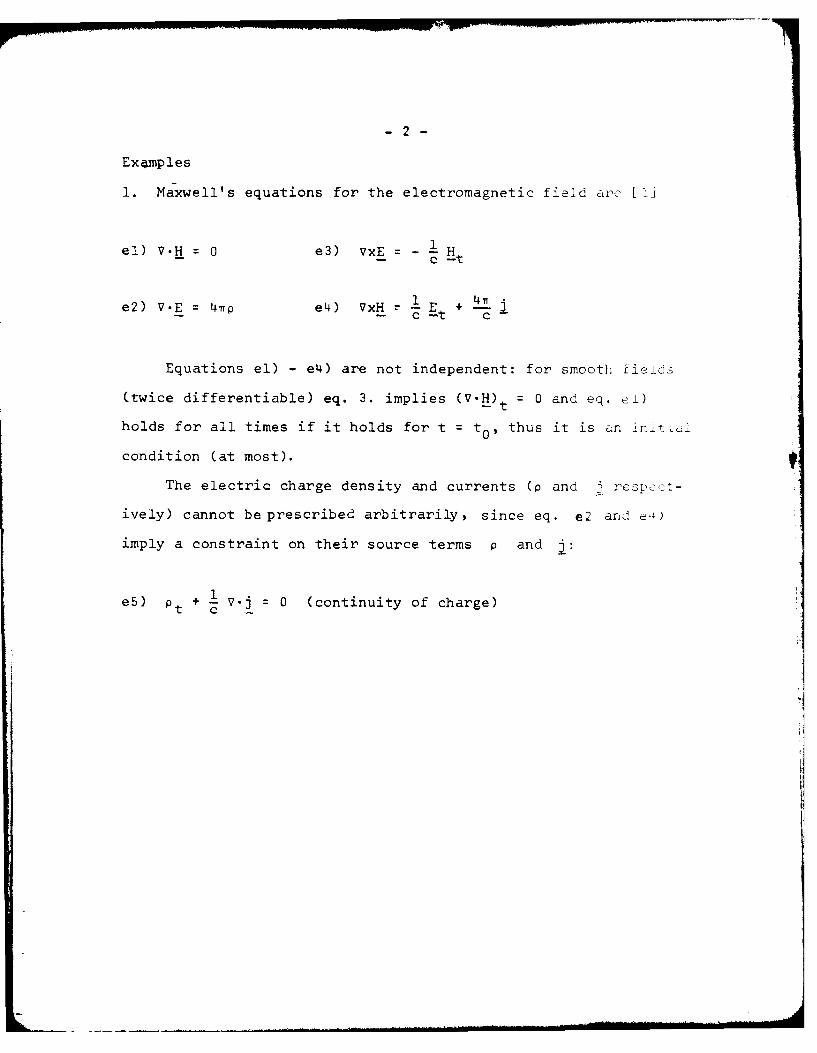
Ex ump les

1. Maxwell's equations for the electromagnetic field are [I

el) V.H = 0 e3) VxE = --

e2) V.E = 4fp e4) VxH r -

Equations el) - e4) are not independent: for smooth ±ieids

(twice differentiable) eq. 3. implies (V.H) t = 0 and eq. ei)

holds for all times if it holds for t = to, thus it is an inli tL.i

condition (at most).

The electric charge density and currents (p and j respect-

ively) cannot be prescribed arbitrarily, since eq. e2 and e,)

imply a constraint on their source terms p and i:

1,

e5) p~ + -1 V-j 0 (continuity of charge)t C

;I

-3-

II. Steady-state Aerodynamics

for which:

(XlX 2 ,X 3) (x,y,z) - space coordinates

u (Ulu 2 ,u 3 ) (u,v,w) - velocity components

A pu

and: P p(u2) density

G 0, W W(x)

where: W 0 for irrotational flow, but changes across ovxe.

shocks. Spelled out in Cartesian coordinates we get:

e6) (a2-u 2 )u + (a2-v 2 )v + (a2 _w-w2 )wz - 2uwwx - 2uvvy - 2vww 0,

(i) w - u~ : W(I )

(3)(it) w~ - v W

(iii) - v = W

i.e. 4 equations for the 3 unknown functions (uov~w).

4-

Methods of Solution and Descretization

The system equations (1), (2) even when simplified for

* specific physical field, is multidimensional and coupled, which

renders it complicated to analyse and inconvenient to solve.

Auxiliary functions (e.g. scalar and vector potentials)

have been taylored to simplify and clarify the mathematical

picture and render it elegant, intelligible and solvable.

For irrotational fields u, i.e. W 0 eq. (1) reduce to

one second order equation for the scalar potential 4, defined by:

u = VO, so that eq. (2) is satisfied identically.

Fc. Maxwells equations the standard analysis is done via

the scalar and vector potentials: 4 and A respectively, (e.g. fIj).

where:

1AE -j V , H = VxA.

Written in terms of (4,A) Maxwell's system reduce to 4 equaic'ns

f3r the 4 components.

The resulting equations are higher order, and admit a wider

family of solutions, all equivalent under gauge transformations:

f ft(x,t)

c t

A' A + Vf

-5-

or in 4 dimensional notation:

(A,-O) + [vf,- f

The potential formulation for the electromagnetic field is

endowed with a beautiful structure, lucid transformation prop-

erties and striking accessible information content (e.g. de-

coIpling into n d order wave equations for each of the components)

unfolding the wealth of electromagnetic waves ref. [i].

Another suggestion, to equalise the number of equations and

unknowns is to add a new dependent variable:

v = V.u

and using the relation:

VxVxu = V(V.u) V 2u

replace eq. (2) by its rotor:

(4) 72 u = Vv - VXW,

which, with eq. (1) gives (n+l) equations for the (n+l) unknowns

(u,v).

The formulation above has been suggested by M. Mock for comnpu-

tational purposes, with a staggered mesh for (u,v) (to avoid decoup-

ling of the descretized equations for u and v) to solve boundary

value problems.

-6-

Direct field formuldtion

The auxiliary function is (e.g. potentials) formulations

invariably raise the order of the equations to be solved; the

first-order system becomes second-order. This requires a higher

degree of smoothness for the solution function and may be a

draw-back for numerical analysis and calculations. Thus, although

many large computer simulations are based on 'potential' formu-

lations (e.g. ref [2]) a direct solution of the first order sys-

tem has been found beneficial [3]. Sometimes essential [4],

.especially for 'initial' rather than boundary value problems.

The question is how to choose the 'right' (n-l) rotationality

conditions that will give with the continuity eq. (1), the 'right'

(nxn) system for a stable descretization for a marching scheme

to solve the first order system, to obtain directly the n field

components (so-called primitive variables), A simple treatme,:

for irrotational, 3-dimensional fields (worked out for the prob-

lem in 4 43) is given in [si. It is extended here for the gener:1

case (eq. (1), (2)), where the field may have sources and be

-otational (e.g. an electromagnetic field with moving charges,

flow behind a curved shock, motion of reacting gases.)

- 7-

Choice of Equations for 3-Dimensions

Spelled-out for 3 dependent variables and 3 independent

ones (e.g. Cartesian space coordinates) we get:

x = (x 1 ,x 2 ,x 3 ) = (x,y,z)

u = (Ulu 2 ,U 3 ) = (u,v,w) (x,y,z)

A (A ( ) , A ( 2 ) , A ( 3 ) ) (u,v,w; x,y,z)

and the system of equations is:

(I) A () + A (2) + A (3 Gx y z

W - V Wy z

(2) u -w 2 )

I

v - u W W( 3 )

x y

i.e., 4 equations for the three unkonwon functions (u,v,w), a

redundant system for a well defined field.

In addition, a compatibility on W requires:

3) ( ) + W ( 2 ) + W = 0x y z

-8-

via which 2 components of W determines the dependence of the

third on its corresponding coordinate, e.g. when W (2), W(3 ) are

given, the following must hold for W(1)

w() -(w(2) + w(3))x =-y Z

( 1 ) : - I x (W(2) + W(3)) z ME + W ( Xo{F z

x0

e.g. i) w - v - Wy z

ii) uz - wx = 0

iii) v - u = 0Zxy

(3) W ( ) 0x

or: W(1)(xyz) W ()y,z) + C

((i):W~l (x = XoYSz)

Thus W( 1) cannot be a function of x and along x-lines re-

tains its value at one point: x = x0 . The non-zero component

of the vorticity is constant along lines parallel to the

corresponding coordinate.

9

Irrotational Fields

In this case W= 0, eq. (3) is satisfied automatically and

equations (2) become:

i) w -v = 0y z

ii) u -w = 0

iii) v -u= 0x y

for (u,v,w) (x,y,z) unique and sufficiently smooth, (e.g.

twice differentiable in each of the independent variables) we

get:

ii) -7 0= u -z Wx CUy) ( Wy)x vx)z - (Wy)x CVz-Wyuz y z y x x z y x y x

!'x (ii) (u,w) E C2 i) vEC 2

v - w : c(y,z)

For u irrotational at any x n ,

(vz-w )XoY,Z) = 0 - C(y,z) 0 C(yz)

and i), ii) - Ciii) which can be considered-and "initial condition"

at most, (e.g. x0 -> - , and a uniform field there). in exactly

the same manner:

[U ~ ~ i0 w-i) iii) ->' [Uz-.W Iy = 0 -1

u-wy = F(x,z)

and irrotationality at any y = y0 plane implies F 0 and eq. (ii)

and:

i) ii) -> [v-u I = 0xy z

and irrotationality at any z = z0 implies iii).

Thus any of the 3 irrotationality conditions implies the

third, for unique smooth, irrotational fields everywhere. For

stable numerical algorithms however, one has to choose set that

carries the appropriate "boundary information" along the ndrch-

ing coordinate; if the integration is to be carried out a!cng:

the xi direction, the ilh component of the iirrotationality

equations has to be omitted [4] , [5].

- ii -

For the general irrotational Case:

(i) W - v Wy z

(ii) U - W W2)z x

(iii) v- u W Wx y

(3) W(l) + W(2) + W( 3 ) 0.x y z

Differentiating and substituting we get:

7x. i) W -x Vx

( w - -W I

z y x x

(zy W( ) + W(12 W

y xz x y

(iii)

V - u W (3) + F(xy)

x y 0 0

Thus i) ii) -> iii) provided vx-uy is given at z : z0.

In the same manner each two of the equations determine the

third, for which initial conditions have to be given for uniqueness.

- 12 -

Algebraic treatment

Equations (1), (2) can be written in a matrix form (used

widely for numerical analysis and descretizations):

(5)

Au A§2)u w u v w!U

0 0 0 v + 0 0 ± v + 0 -1 0 v

0 0 -1 % 0 0 0 w 1 0 0 1

0 0 -1 0 0 0 0 0_

3 ()

i i

w(l)

w( 2 )

wC(3)

or in short:

C(X) u + C(y ) u + c(Z)u 2 F

with the corresponding (4x3) matrices C and 4 forcing functicns F.

- 13 -

The system C5 is again redundant, and one of the last _

equations has to be deleted to render the (4x3) coefficient

matrices C into (3x3) matrices . The choice is directed

by the marching "time like" direction, for which the M(i)

matrix has to be invertible, hence nonsingular, hence with

no row (or column) of zeros. This automatically rules out one

equation: when (u,v,w) are given at x = x0 (e.g. x0 _> -G

for steady flow about an obstacle), the first irrotationality

condition has to omitted. A marching procedure along the x

axis requires the inversion of the non-redundant matrix (x)

such that:

u -_[ (x)]-l (Y)u +( (z) + [ 1Fx)]-i1

-- y --

In the same manner, integration schemes along the y anrd z

directions require the omission of (5i0 and (biii), respective1 ,

as a necessary condition (not always sufficient.) for a well

defined, stable scheme, (as is seen in [4]).

- 14-

Final Remarks

The question and system treated are elementary and so gen-

eral, the analysis and answer so simple,to be judged trivial,

if not for the fact that the question does come up occasionally

(e.g. [4]), and the answer not always immediate. Essentially

the same problem has been treated recently (and has come to

our attention while writing this note), in a completely differ-

ent context for different reasons and aims in [6]. It also seems

to be related to other recent approaches [7] and to variational

formulation and analysis of the system at hand with related

physical applications t8].

Work on relaxing the smoothness requirement, re-formulation

and analysis for non-smooth fields (e.g, flows with shocks) is in

progress.

4.

- 15 -

References

[i] Mechanics and Electrodynamics, a shorter of theoretical phys-

ics, Vol. 1, L.D. Landau, E.M. Lifschitz, Pergamon Press,

is ' ed. 1972.

[2] Numerical calculations of Transonic potential flow about wing

body combinations, AIAA Journal, Vol. 17, No. 2 1979, pp.

175-181.

[3] Finite Element calculation of steady transonic flow in

nozzles using primary variables, J.J. Chattot, J. Gruin-Roux,

J. Laminie.

[4] Shock-free wing design, K.Y. Fung, H. Sobieczky, R. Seebass,

AIAA 79-1557, 12th Fluid and Plasma Dynamics meeting,

July 1979. (eq. (4) and discussion)

[5] Finite Elements for Fluidynamics, N. Geffen, Finite Scienti

fic Report, Grant No. AFOSR-77-3345, July 1979, pp. 15-16.

[6] Redundancy and Superfluity for Electromagnetic Fields and

Potentials, J. Rosen, to be published in the Am. J. of Phys-

i cs.

[7] Ideal gas dynamics in Hamiltonian form with benefit fc:r

numerical schemes, 0. Buneman, to be published in the Phys.

of Fluids; also a presentation at the 7th International

Meeting on Numerical Methods for Fluid Dynamics, Stanford

and NASA Ames, June 1980.

[81 Alternative variational formulations for nonlinear vectcr

systems, N. Geffen. This report.

II. ALTERNATIVE VARIATIONAL FORMULATIONS

FOR NONLINEAR VECTOR SYSTEMS

Nima Geffen

Abstract

Variational formulations for vector fields described by a

system of partial differential equations of whatever type, possit-

ly nonlinear, and with initial-boundary conditions are given.

Smoothness properties of suitable approximation spaces are viewed

and the effect of coercive ,natural boundary conditions dis-

cussed briefly. Examples are drawn from electromagnetic field

theory and fluidynamics.

Differential equations

Consider the following conservation and rotationality condi-

tions, for a vector field u(x):

(1) v*V = G

(2) Vxu W

(3) u(x) = f(x) x E M:

where:

u = u. is the vector of dependent variables i = 1,...

x = x. is the vector of independent variables j :1,...,n

G = G(x) is a given function

W = W.(x) is the vorticity

V = V. (X,U)

The vorticity W has to obey a compatibility condition:

(4) V.W : 0

The system of equations (1), (2) is quite general, it can

be linear and nonlinear, elliptic, hyperbolic or mixed with smocth

or non smooth solutions. The independent variables xi may

designate space and time coordinates and different kinds of

initial and/or boundary conditions may be appropriate for differ-

ent problems. Higher order equations may be put into this form,

and examples of applications include the description of electio-

magnetic fieJd s, "e theory of elasticity, fluidynamics, and plasn.,-

dynamics, including flows with shocks.

U

-2-

Variational Formulations

A variational formulation of the field u satisfying (1),

(2), (3) is a functional J(v) defined on S1 whose stationary

value is obtained for v u:

6J(v) = 0 < v = u

For well posed problems, for which u(x) is unique

6J(v) = 0 0 v = u

Variational formulations are scalar, short, additive (the

functionals for complex systems are direct sums of their

simpler parts), invariant under appropriate classes of tran,-

formations and are often convenient for theoretical analysis

and for numerical simulations, e.g. by the finite elements

method. Integrals can easily be descritized and approximated,

and the smoothness requirements on the functions are less strirn-

gent than for the corresponding differential system. This last

point is most important from the numerical view point in addition

to a better rationale for the treatment of shocks.

The case G = 0 is described in [l]. The functional J(v,x):

J f L(v,x) + X.(Vxv-W) + J Xxv-dG is stationary:

m

6J(v) = 0 at v = u

provided that: V x v 0.

V L-- U

resulting in:

V = -Vxx

The variation is done on all v for which J is defined

and v satisfying coercive boundary conditions on the bcundary'

9. - or for which X II v or vilda on 32.1 m

For the non-sourceless (or sourceful) case; the following

variational statements hold:

Th. i

The functional:

(5) J(v) [L-y.v + A(Vxv-W ].dx + j Axv-da

m

is stationary for v = u satisfying (1), (2), (3) providec .-Zb2t

(6) V x V 0

where:

(7) V. : G or = V-IG

(8) V = V L-- U

f4

(9) V =VX-X +

v is allowed to vary over all functions for which (5) is

defined and finite and which satisfy the coercive B.C. (3).

The proof is straight forward and follows the details in [1]

exactly.

_____- 5-

Corollary

The functional:

(10) J(v) = (L-F&.v + X-W)dx + fXxv-da (3)

m

is stationary for v u satisfying (1), (3) when the variation

is taken over all fields satisfying eq. (2) and the initial/bound-

ary conditions (3): i.e.

6J(v) = 0 < v u : v.V = G

VxV = W

-j .&.j(x) xE3ai

The restricted variational statement (10) follows from the

statement in (5) by inspection.

-6-

An alternative formulation is obtained by integrating the

2nd term by parts, using the vector identity:

V.(Xxv) - v. VxA - A. xv

substituting in (5):

)-Vxv = v.Vxx - V.(Xxv)

Th. 2

The functional

(11) J(v) - (L-.v + v.VxX - X W)dx

is stationary for

v = u satisfying (1), (2).

In the variational formulation (11) is made over all v

in which render all terms integrable. The lagrange multi-

plier X is required to have integrable first derivatives, which

appear explicitly in J.

The surface term drops out, and the solution v = u satis-

fies the natural boundary conditions: Xpu or ull dc; or. a2

Smoothness requirements

In the variational formulation (5) v is required to be

at least once differentiable (for the 2n-d term to be defined)

which holds also for (10) (where eqo (2) has to be satisfied).

The lagrange multiplier A in this formulation can be just inte-

grable, e.g. a step function. The variational statement (11),

on the other hand, does not involve derivatives of v (hence

admit integrability - only there) but requires A to differ-

entiable at least once. Formulations (5), (10) include a sur-

face term and involve spaces satisfying appropriate boundary

conditions; in statement (11) the surface term has dropped out,

and the solution v = u making it stationary satisfies a natural

boundary condition. Both smoothness requirements and behavior cn

the boundary has bearings on approximation spaces used for numer-

ical calculations, and on the stability of numerical schemes.

Simple examples are described in the following part of this reourt.

[2].

-- 8----

-8-

Examples :I. Steady electromagnetic field

Maxwells' equations for a steady state can be written w [ 31

i) V'E z p ii) VxE = 0

iii) V.B = 0 iv) 7xB = j

A variational statement for i) ii) is:

(5W) J(E) =I( 2 2yE) + (E)(VXE) + f A (E)xE.d

for E arbitrary, or:

(10') J(E) 7 (EL/2 - g-E) for E irrotational.

where: is any solution to

V'g= p or: V -p

The variational statement (11) for i) ii) become-:

(11') J(E) E [E2/2-g.E) - E.(Vx )]

The corresponding variational formulations for the nagncta2

equations iii) iv) are:

-9-

(5") J(B) B' /2 + (B) 7 xB-i) + f (B)XB_'do

(0") J(B) IB '2- A j + I xBdo

ni

for B satisfying eq, iv)

and

(11") J(B) L [B2/2 - B.(Vxx(B))]

the functionals for the combined field are obtained by simply

adding the ones for the 'separated' system:

(W ') J(B,E) = [- . + 2 B.2 ++ k(E)(VXE) A (B) VX) + E xE d l

(B AxB'd+

r B

(10"') J 2 - .E + .j +

for irrotational E and B satisfying iv).

The statement (10") can be reduced to the one used for the sca. i:

and vector potentials for the irrotational electric an" aoleni:ii-

al magnetic fields, (e.g. [31 pg. 366 eq. (11-65).

i

- 10 -

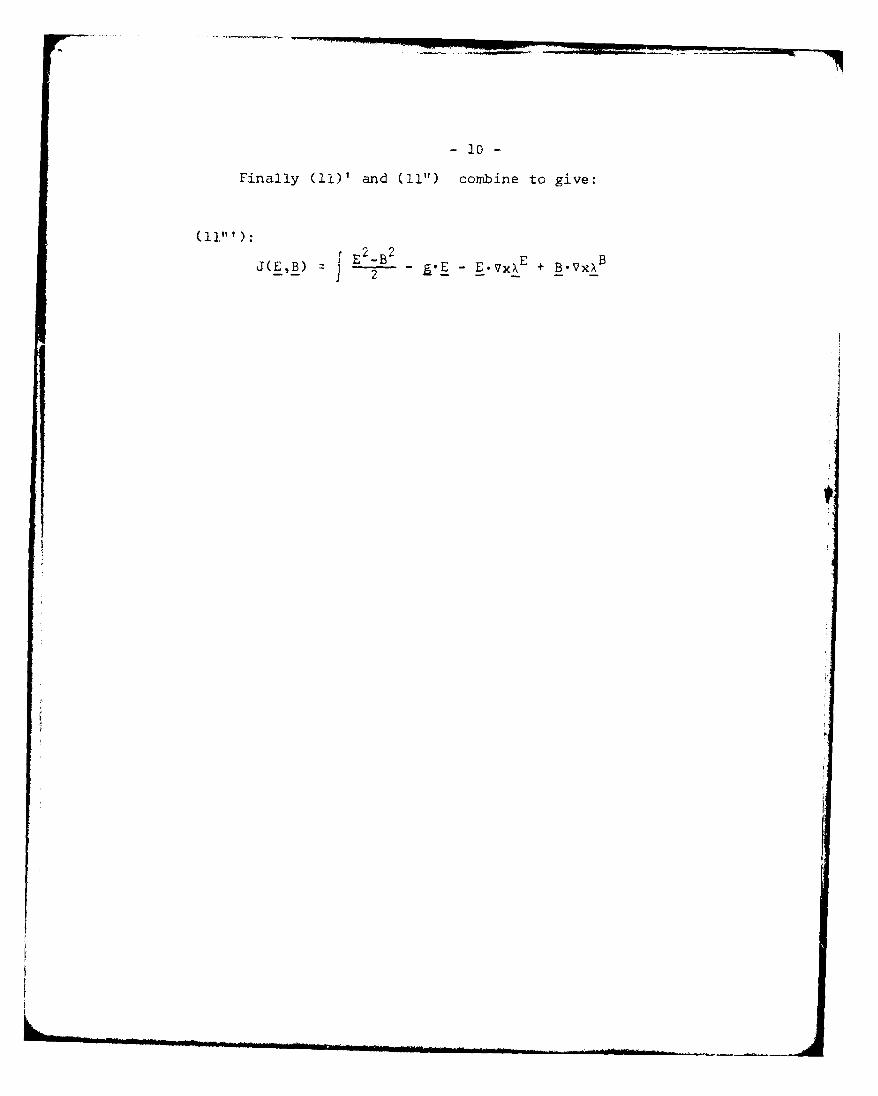
Finally (11)' and (1i") combine to give:

(11"'):

J(EB) E 2_2 E - E.vxXE + B.VxAB

2 Fa

- ii-

2. Steady fluidynamics

The differential equations are:

V-(pq) = 0 p = p(q2)

Vx-q: w

and the corresponding Lagrangian L and functionals are:

PUor: Pu a- au Vui ui

J(u) I[L + .(Vxu- w)] + Xxudo

(iA) or:

J(u) L - X • w + A x u-do

or:

(11) J(u) = L - x-w + u'7xx

for the appropriate function spaces, with the required smooth-

ness properties, and constraints in the region and/or' on the

boundary.

The results () have been described and analyzed in [la], [ib]

where applications to specific flows are given; the formulatifn

-12 -

(lb) of a slight modification used in electromagnetics and other

field theories but not generally useful for computations due to

the practical difficulty in actually constructing a wide enough

family of v fields that satisfy the rotationality condition (2)).

The formulaticn (1) is new and can be readily specialized to par-

ticular fields; it offers an interesting alternative from the

theoretical point of view but holds rather doubtful promise compu-

tationally (stability problems?).

- 13 -

Concluding Remarks

A preliminary report on alternative variational formulations

is given for general vector fields governed by systems of

partial differential equations, possibly nonlinear specifying

their sources (eq. (1), e.g. conservation of mass for G = 0)

and vorticity (eq. (2), e.g. w = 0 for irrotational fields).

This framework is pregnant with information and connections

with other variational approaches and with related mathemati-

cal and computational questions. It also involves the questions

of redundancy symmetry and the appropriate way to describe

these fields for the continuous and non continuous cases,

which may (and most often wiil) occur for nonlinear systems,

e.g. flows with shocks.

The last question as well as the elaboration on the othei

points are in the works now, to be reported at a latex, oaze.

Simple computational examples, rnerc.,natiye f r ,U-

lations and trial functions are used for the Laplace and rri-

comi problems are reported in the following chapter,.

- 14-

References

[la] A variational formulation for constrained quasilinear

vector systems, Nima Geffen, Quarterly of Applied Mathe-

matics, October 1977, pp. 375-381.

[1b] Variational formulations for nonlinear wave propagation

and unsteady transonic flow, Nima Geffen, ZAMP vol. 28,

1977, pp. 1038-1043.

[2] On different mixed finite element approximations for

elliptic systems, S. Yaniv, this report.

[3] Classicai Mechanics, H. Goldstein, Addison-Wesley, 1959,

§ 11-5, pp. 364-370.

III. ON DIFFERENT MIXED FINITE

ELEMENT APPROXIMATIONS FOR SYMMETRIC

ELLIPTIC SYSTEMS

Sara Yaniv

Abstract

Different finite-dimensional spaces are tried for mixed

finite element approximations for a functional which has a

saddle point at the solution of elliptic symmetric linear syster.,

with a Lagrange multiplier. Calculations are carried out for 2

first order equations, (u,v)(x,y) and boundary conditions, e.g. .

Laplace and Tricomi's problems. Brezzis' convergence condition

is found hard to verify rigorously, even for descretizations that

seem to work well. Preliminary analysis is tried and experin.i-:,s

conducted for bilinear variations on rectangles for all ccmpon-

ents and for bilinear (u,v) and piece-wise constant (A) trial

functions.

-2-

1. Introduction and variational formulation

Consider the equation

(1a) A x+ By : f(x,y) (A,B)(x,y, ~ X'

in a domain 2 with given boundary conditions:

(1b) A)0

Assuming

U x

V

and A ~Bu

then the operator F(x,y,u,v) A x B Yis a potential [I, I,-.

The variational formulation for the problem is: find (;-,v;A.)

so that

(2) J(u,v;x) r[~~yuv + X(u -vx)]dxdy

2 2JF(x,y)udxdy

F(x,y) fX f(&,y)dC

is stationary, for all functions (u,v) E VxV and E . w),,er~e

-3-

e ecy (Uiv) E VxV satisfying boundary conditions:

udx + vdy =0.

7,,,v) is the Lagrangian of the problem, i.e.

and x (x,y) is a Lagrange multiplier which is the stream untr

of the problem [1, page 39].

The variation of J(u,v;x) for fixed Agives the 1Lc

ing weak formulation:

(. j(u,/;X) j[L u6u + L v6v + X(6u Y-6v x )]dxdy 0

A;Icing the equation

u - V = 0y x

ii. weak formulation:

IJ j (uy-vx)dxdy= 0 for VqEW,

we get a saddle-point problem:

1u 1(tta) ofL.u + Lv v + X(- -)dxdy 0

V(,V1 )E V x V

and

(4b) I ) - --)dxdy = 0 VqEW.

The functions u,v and A which satisfy (1a) and (1h) are

the solution of (4a) and (4b).

For linear problems:

L u + L v = A u + B v E L u 2 + 2L uv+

+ L v2

vv

and for an elliptic equation it is positive definite form.

Hence

VxV = {(u,v)/f[Luu. u2 + 2Luv.uv + L .v2 +

+ (u Y-Vx ) 2]dxdy < - , udx + vdy 01

2 ff[Luu2 v2+=[uv) I + 2Luvuv + Lv 2 + Yu -V )L]dxdyluv)VxV J uu Lvv

and, since x depends on an arbitrary constant:

W = {q/J fq2dxdy < - , q(xoYo) 0)

(x 0 ,Y 0 ) E S.

j

This formulation gives a saddle-point problem [2], which is

determined as follows:

Given f E V', g E W', find u E V, * E W such that:

a(u,v) + b(v,*) = f(v) VvEV

(5)

b(u,o) = g(o) VEW

Brezzi's theorem states the following conditions for

existence and uniqueness of the solution:

Suppose a and b are bounded and

(6a) inf sup ja(u,v)I > > 0uEz vEz

ijuliV = 1 IOv IV = I

z £ {uEV/b(u,4) = 0 VOEW}

(6b) sup Ib(v,')l > k 4IIu VJEW, k > 0vEV Il vil V

then the solution of (5) is unique

and

fluif V + hIt W < C( OfIIv , + IgOwl,)

It is easy to verify that problem (:a), (4b) satisfies

(6a), (6b), (6c), hence has a unique solution which is the only

solution of (ia), (lb).

2. Approximation

In order to approximate the solution of problem (4a), (4b)

using the saddle-pc:int weak formulation or the saddle-point

variational principle, we use finite-dimensional spaces Vh V,

Wh c W satisfying:

(7a) inf sup ja(uv)I > -r> 0 , r independent of huEZh vEZh

lull V:I l 1 V: I

(7b) sup ia(u,v)I > 0 V 0 1 u E ZhvE Zh

Z {uEV; b(u,O) = 0 VYEW}

(7c) sup Ib(v,' )i e 11 11vV h [IV 11V

VYpEWh

k > 0, independent of h.

The approximated problem is:

a(uh,v) + b(V,41h) = f(v) VvEVh

(8)bMuho ) = g(¢) VOEW h •

Under hypothesis (7a), (7b), (7c) problem (8) has a unique

solution [2] and:

u- Uh V +i - WhI < c inf (lU-Xl +XEVh

6E Wh

-7-

3. Examples

We used the variational principle (2) to solve, approximately.

the Laplace equation and the Tricomi equation in an elliptic domain.

i) The Dirichlet problem for the Laplace equation

¢xx + yy = 0

I ail f(x,y)

The variational functional is:

(9) J(uv;X) = f(u2 + v2 + X(uy-v x)]dxdy

for (u,v) E VWi? , E E W

VxV M {(u,v)/ if(u 2 +v2 +(uY-vX)2 Jdxdy < -, udx + vdy dj

W: {q Iq2dxdy < q(x 0 'Y0 ) = 01

for this problem conditions (6a), (6b), (6c) are fulfilled,

hence the problem has a unique solution.

Let Q be the rectangle:

{Cx,y)/ -i . x . 1, -1 . y . 01.

-8-

We have divided Q into rectangles of size h and chcsen dif-

ferent finite dimensional spaces for the trial functions

a) The first attempt was to use the bilinear trial func-

tions for (u,v) and X, for these spaces Brezzi's conditions are

not, necessarily satisfied; this is concluded from the instability

of the numerical solution, in some of the cases tried,

b) We tried to take other finite dimensional spaces so that

(7a), (7b), (7c) will be satisfied. Using the same finite-element

discretization of 0 as in a), approximating u and v by bilir.-

ear trial functions and piece-wise constant functions for X

(intuitively, this may help to get rid of the 4 constants and

leave us with the only arbitrary constant of the problem which is

q(x0,Y0 ) = 0).

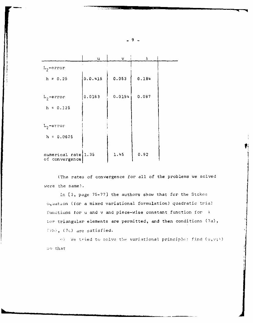
For this approximation the solution converged to the analyti:

solut ion;

u - ex siny, v cx cosy, A -2e cosy + 2/e 1 as shown in the

following table:

-9

u v _

L - error

h =0.25 0.0.415 0.053 0.184

L 2 -er'ror 10.0163 0.0194 0.097

h =0.225

L -error2

h 0.0625

numerical rate 1.35 1.45 0.92of convergenceII

(The rates of convergence for all of the problems we solved

were the same).

in [3, page 75-77] the authors show that for the Stokes

_-4.udtiofl (for a mixed variational formulation) quadratic trial

_runctions tor' u and v and piece-wise constant function for X

for triangular elements are permitted, and then conditions (7a),

0!:, (70) are satisfied.

~)We t~ried to ,3olvc the variationial princip~e: find Cu ,v;'

_ir thait

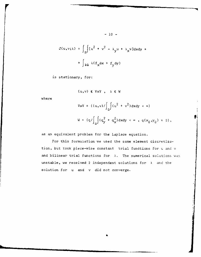
- 20 -

J(u,v;X) f f Cu2 + V2 - yu + X x v]dxdy +

+ Afa A(fxdx + f ydy)

is stationary, for:

(u,v) E VxV , E E W

where

VxV = ((u,v)/ JJ(u2 + v2 )dxdy <

W = {q/irj q 2~ + q 2)dxdy < q=,,,

as an equivalent problem for the Laplace equation.

For this formulation we used the same element discretiza-

tion, but took piece-wise constant trial functions for u and v

and bilinear trial functions for X. The numerical solutions was

unstable, we received 2 independent solutions for X and the

solution for u and v did not converge.

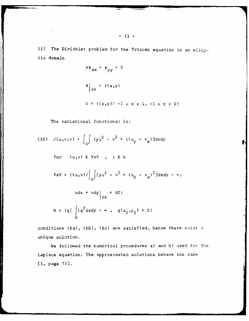
ii) The Dirichiet problem for the Tricomi equation in an ellip-

tic domain

y¢ - =0YXX 0yy 0

€1 : f(x,y)

Q = {(x,y)/ -l < x i, -l . y .C 0}

The variational functional is:

(10) J(u,v;A) = ] F (yu 2 - v 2 + X(u - v )]dxdy

for (u,v) E VxV , E E W

vxv= {(U,v)/Jf[yu2 v2 + (u-ldxdy <

udx + vdy " df)

W- {qj I(q2dxdy < , q(xoYO) 0)

conditions (6a), (6b), (6c) are satisfied, hence there exist a

unique solution.

We followed the numerical procedures a) and b) used for the

Laplace equation. The approximated solutions behave the same

[1, page 73].

- 12 -

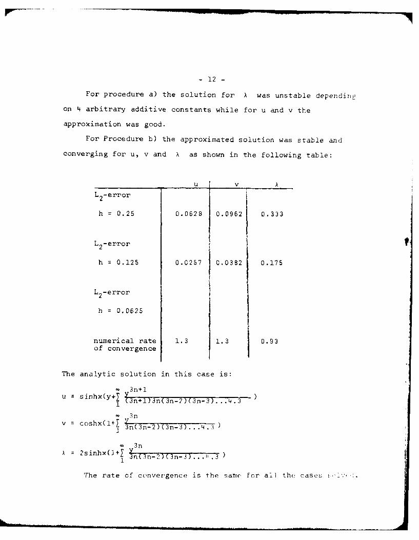
For procedure a) the solution for A was unstable dependir-'

on 4 arbitrary additive constants while for u and v the

approximation was good.

For Procedure b) the approximated solution was stable and

converging for u, v and X as shown in the following table:

u_ I vL 2- error

h = 0.25 0.0628 0.0962 0.333

L2- error

h = 0.125 0.0257 0.0382 0.175

L 2- error

h = 0.0625

numerical rate 1.3 1.3 0.93of convergence

The analytic solution in this case is:

003n+1u = sinhx(y+l y32l1 (3n+l) 3n(3n-2")(3n-3)... 4.3

3nV =Coshx(l+l Vv csh~l 3 n(3n-2)(3n-3) ... 4.,T)

3nA =2sinhx(l+ n_

3nc3n-2)(n-3) ... h.3 )

The rate of convergence is the same for all the cases ~K

- 13 -

4. Remarks

Equation (la) is equivalent to the first order, system:

L -A = 0u y

(11) L + A = 0v x

U -v 0

y x

where

L = 2u for the Laplace equation

L = 2vv

and

L = 2yu for the Tricomi equation

L =-2vv

It is obvious that the solution for X has more derivativec

than u and v.

The trial functions used in procedures a) and b) do not

satisfy this feature while those of c) satisfy it. But the only

procedure which gave a converging solution is b).

The only conditions which insure convergence of the approxi-

mated solutions are those of Brezzi (7a), (7b), (7c), (which are

quite difficult to show in the finite-dimensional pi-,oberm).

- 14 -

Summary and Concluding Remarks

A summary of results i :rnite elcernt e - . ."

non-uniformJy ellipt.c pj:s t- eiven ,.

gion is descretized in to rect an, f:, '

assumed for both field variilles j n,) 11nOi tie Lo ':o.gc:: ;.:-

A appearing in the functional:

[ J L + .(u - ,' j ] dxdA

(12) Jtu,v;x) [Lc +v y (

to be made stationary at the >oiu~iou Zuncti jr§ luv:

The values of A at one c,. mc :,. -. "

mine its values :t even points only ,rn t:,e t

the odd points consist of :p tre :ys:r!,,

ceptable behavior of the overall ;oJil-cn (.a ... :.......

other computational contexts). To coup.Le the eq,>:t : :

points the values of kat the 4 points at the .A ,_

had to be predetermined (e.g. by 0 Taylct' eV:s......

(0,0) point and the relation to the values ..

rectangle). The procedure is not con,:ci erea sat 7....

it yields acceptable resu]is. On the nypeIcl I

intermittency ca,-sing unstability has been ,s- v,

Following a series ol lectures y J. Cihoxn [ ..

variation was retained Icr. (u,v) but te t, -, "

replaced by piece-wise constants -.ri :t rngl's.

occurs and the calculat ion: are .z on,-2 Ite ly at ib. ;ia .' .

- 15 -

The price is paid in a lower accuracy, but the scheme is neve:-

theless considered feasible.

The functional:

J(u,v;x) = I [L + ux - vX ]dxdy + f X(fxdx + fy y)

I dobtained from (12) by integrating the 2L- term by par-s, iz

also stationary at the solution to the Laplace system. The sa.'-

descritization and the corresponding trial spaces yield un-:'>

scheme, This is somewhat unexpected, because the relative di -

entiability required for (u,v) and A in (11) fits better the

analytic relation than the one in b). The stability analysis

for this case (via rezzi's coetclvity condition for the a -

mation spaces) i-I difficult, dnd wt, have not been able c .

it to a successful ccnclusion.

- 16 -

References

[I] S. Yaniv, Variational formulation for formally symmetric

problems and it's application to the Tricomi equation,

Ph.D. Thesis, Tel-Aviv University 1978.

12] F. Brezzi, On the existence, uniqueness and approximation

of saddle-point problems arising from Lagrange multipiiers.

R.A.I.R.O. (8c ann~e, aoQt 1974, R. 2, p. 129-151).

[3] V. Girault, P.A. Raviart, Finite element approximation of

the Navier-Stokes equation, Springer-Verlag 1979.

[4] J. Osborn, Series of Lectures: On Mixed Finite Element 1'elh-

ods, and private communications, Tel-Aiiv Universiiy, J_. i')E,.

IV. FINITI EIYi:> LX. AiPROXIMATIONS FOR THE

SOLUTIN' CF I11:. TFICOM,"I EQUATION IN A MIXED

ELLIITIC-HYPERBOLIC REGION

by

David Levin

Abstract

Difference schemes foi te sclution of the Tric,,i _ :

are derived, in both the tlliptic u- hyperboiic:air.

schemes are constructed so to be exa.ct fI. several v.cv .,.

solutions of the Tricomi ejuaticn. The method presented is

adaptable to non-) ! I I,:- arnd to non-st Cndazd re2 .

A high accuracy is dcemwst ri e 1 I .ever.Ii Tricoi c,-i~i v

conditions.

1. Introduction

The Tricomi equation

Sxx C (.)

is elliptic for y < 0 and hyperbolic for y > 0 wit.h ch-

acteristics defined by:

3/2= X + -V

2/ (1.2)

Tricomi [6] showed that (1.1) has a unique solution in a

domain D = D+ U D- bounded by a ,simple arc r- in the ellip-

tic domain with endpoints on the x-axis at x = A and x =

and by the two characteristics . and F ) through these

endpoints (figure 1.1).

Figure -.

r r

-- - - - --

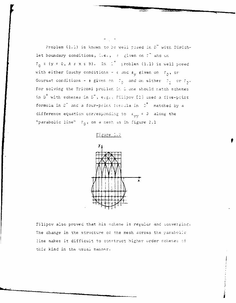
Problem (1.1) is known to 'o well pzsed in L- with Dirich-

let boundary conditions, o.e., :iven on F- anc cin

S{y 0, A < x 1 B}. In -roblen: (1.1) is well posed

with either Cauchy conditions - a and y given on or

Goursat conditions - g given nr and on either cr o _

For solving the Tricomi probie> iN I one should :a t h scheres

in D with schermes in L , e.g. iovizcv [1] used a five-point+

formula in D- and a four-point fox>:- la in D matched by a

difference equaTion ccrrespznding to , 3 along the

"parabolic line" , on a mesn -s in figure 2.1

Fi gure _

Filipov also proved that his scheme is regular anc 2onverinig.

The change in The structure o± the mesh across the parabolic

line makes it difficult to construct higher order schemes <

this kind in the usual manner.

-3.

Another strategy for solving the Tricomi problem is that

of Vincenti and Wagoner (7] who reduced the problem to a pure

elliptic problem. However, the boundary conditions on ro,

which are obtained by projecting the given conditions on F1,

are quite complicated and cause great numerical difficulties.

Several authors, [2], [5] have used expansions in terms of

certain particular solutions of (1.1), and this method proved

to be quite effective for cases of very smooth boundary condi-

tions.

The method presented in this work combines somehow the

motifs of the above three strategies; a local expansion in

terms of particular solutions of the Tricomi equation axe uzed

to produce high order difference schemes for the Tricomi

problem. Using these schemes the problem is reduced tc an

elliptic problem in D with certain boundary conditions on

y = 0.

The method used here for producing the difference

scheme has recently been found to be useful for solving both+

Cauchy and Goursat problems in D It is the versatility of

this method which enables us to obtain specially structured!

difference schemes of high order for the desired matching

along the parabolic line.

In section 4 we describe some numerical experiments with

the suggested procedure, exhibiting a global 0(h 3) accuracy.

2. The expansion method for producing difference schemes

Let zi = (xi,y i ) i 1 1,... ,N + 1 be N + 1 adja-

cent mesh points in a grid covering the domain D. We look

for a difference approximation for the Tricomi equation

N+l(1.1) based upon {z i} . The usual way of obtaining dif

ference schemes is by expanding the approximation u(x,y)

in power series, around ZN+1 for instance, then form a

linear combination of u(zl),... ,u(zN+l), using (1.1), to

get the desired degree of accuracy. This process can be

simplified by using an expansion in terms of the polynomidl

solutions of (1.1). These can be found by expressing

¢(x,y) as a double power series expansion around (0,0) and

comparing the expansions of yo xx with that of yy. The

result is that all the polynomial solutions of the Tric:-.

equation can be written as

x =M-2i 3iP 2 M+1 (x~y) Ic iX y

i=O 1

M 0,1,2,... (2.i)

IP2 (xY) 2 dxM-2i y3i+l

where co = d = 1 and

L ... ....0

-5-

c (M-2i)(M-2i-l)Ci+1 -31 3i3i + 2)

. ,.., . (2.2)

[d. =(M-2i)(M-2i-1) d.i+lJ (3i+4)(3i+3) d

LEMMA.

Let u(x,y) be an analytic solution of (1.1) in a neigh-

bourhood S of (x0 ,Y0 ) then

2M+l MU(X,y) = I a P (x,y) + o((max(h,k) ) V (x,y) E S (2.3)

5=1 j #

where h = Ix-X 0 1 and k = jy-y 01. Also, for y= 0 andk h h2/3

2M+l Mu(x,y) Z bP.(xY) + o(h )

(2 .L)

2M+2 M+2/3I b.Pj(x,Y) + o(h

j=1 j

The proof is straightforward.

Using the above lemma it is clear that if we find a

scheme which is accurate for (P.}N i.e.

NO1 i P j(x i'Yi P S(x N+1,YN+l ),5 1,2,... ,N, (2.S)

then this scheme has a truncation error of order [-] There-

2.

- ---

-6-

fore we simply use (2.5) as the defining equations for our

schemes. This method of obtaining difference schemes is

convenient to use for any given distribution of mesh points,

provided that the system (2.5) has a solution. The method has

recently been used successfully for solving the Cauchy and

Goursat problems in D+ [3]. However, the schemes presented

in [3] are not in a suitable form to be used for solving the

mixed problem in D since they cannot be matched nicely with

schemes in the elliptic domain D . In order to obtain suitaL+

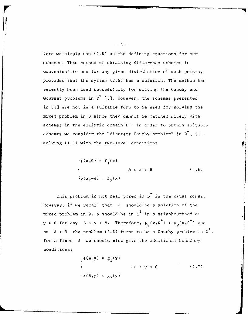
schemes we consider the "discrete Cauchy problem" in D , i.,.

solving (1.1) with the two-level conditions

*(x,O) f1 (x)

A .< x . B (2.6)

¢(x- f 2 f(x)

This problem is not well posed in D in the usual scnsc.

However, if we recall that * should be a solution oI the

mixed problem in D, * should be in C1 in a neighbourhcoe cf0+

y 0 for any A < x < B. Therefore, y (x,O ) y (x,O ) and

as 6 - 0 the problem (2.6) turns to be a Cauchy problem in D

For a fixed 6 we should also give the additicnal boundary

conditions:

1¢(A,y) gl(y)

-6(" Y ,) y < y < 0 (2.7)

-7

to make the problem well posed in A . x - B -6 . y 0, d

hence also in D

For a small 6 it is expected that the domain of influ-

ence of the boundary conditions (2.6) is similar to that of

the Cauchy conditions. Therefore, we consider a mesh defined+

by characteristic lines in D as in [1] and [3]. Hence, we

look for a scheme of the form

M[a iO(xiy m ) + a M+i (x iyYl =(x0 Ym+) (2.8)

m 0,1,... ,2j-i, where

2y 6- 3

Yo = 0 ,

323 23

Ym+l (h + m =,1,...,2N-1

and

x x + h(-I - -) i 1,2,... ,M

where h LA as in figure 2.1.2,

Fiure .

Y A

22 "

The coefficients { i ( .i) are determi v .

with fl 2M, i. e. by tre svste': olf 2,-' eq. r

MS[a.Pxi ,y ) + a, + . ,v )x

r n + -~ 1 (*

Given the "discrete cn ti En ( .)

scheme (2.E) for m = I ( c(.9) 1 i

one can get an ipproxirT,-:t , "I'' level v -

9T

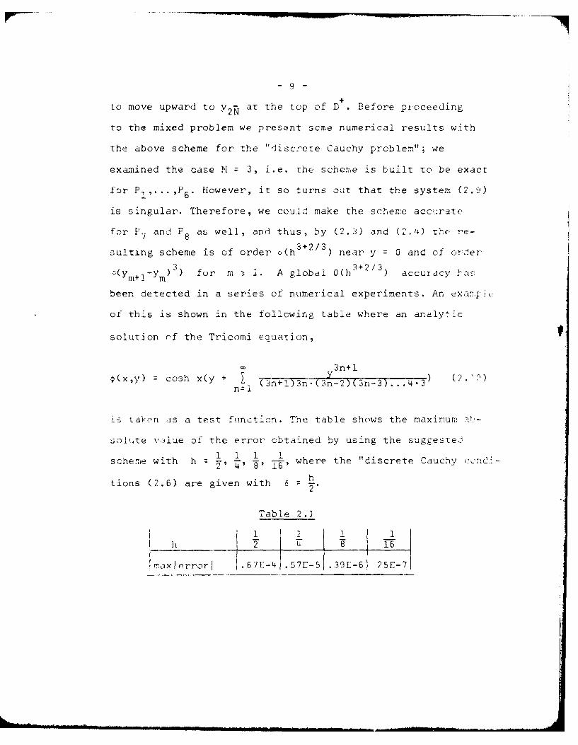
to move upward to y at the top of D. Before proceeding

to the mixed problem we present scme numerical results with

the above scheme for the "disc"ere Cauchy problem"; we

examined the case M = 3, i.e. the scheme is built to be exact

for PI'. ... ,P6 " However, it so turns out that the system (2.9)

is singular. Therefore, we could make the scheme accurate

for P7 and F as well, and thus, by (2.3) and (2.4) the re-

suiting scheme is of order o(h 3 + 2 / 3 ) near y 0 and of order

(ym+l-Ym) 3 ) for m . 1. A global 0(h 3 + 2/3) accuracy a

been detected in a series of numerical experiments. An examp>

of this is shown in the following table where an analytic

solution of the Tricomi equation,

3n+l*(x,y) = cosh x(y + 7 -n+l)3n.(3-2)(3n3)...4.3 ( 2 9 )

n: j

is tak.en as a test function. The table shows the maximum .},-

solute vaiiue of the error obtained by using the suggestej1 1 1 1

scheme with h = 1, 11 -- =-' where the "discrete Cauchy ccnc-

tions (2.6) are given with 6 h h

Table 2.1

1 ] ! 1

laxiorrori .67F-4 .57E-5 .39E-6 25E-71

- -In -

3. The scheme for the mixed problem

We now consider the Tricomi problem in the mixed domain

D = D + U D- with boundary conditions on F- and on r].

Assuming that r is rectangular we can use a rectangular

mesh in D- and 5 or 9 point schemes around any internal mesh

point in D-. The scheme (2.8) for m = 0 can be regarded as

(ifference equaLion for the mesh points on % = 0 However,

when we move on upwards we find that we still miss some diff-

erence equations to stand for the unknowns at the mesh points

on the free boundary F 2 . Therefore, some additional schemes

should be introduced.

Let us denote by p0 the vector of the values of the ap-

proximation at the mesh points on y = 0 and by o_ I the w&c-2N(M-I)-I

tar of the values on y :(--i.e. l)-o) i} anl

2i =-) where

{ 10i iM- i 1 ,... ,2N(M-)-l. (3.1)p (A + ih 0)

•h

'cli : (A + 'N-i- -

Successive use of the schemes (2.8) for m C,l,... ,2N-1

finally yields a linear relation between the approximation at

the mesh points on F and 0 0 and (P_ in the form:

(A+- h,'1 ) = ST .T

7 0 1

M 12*

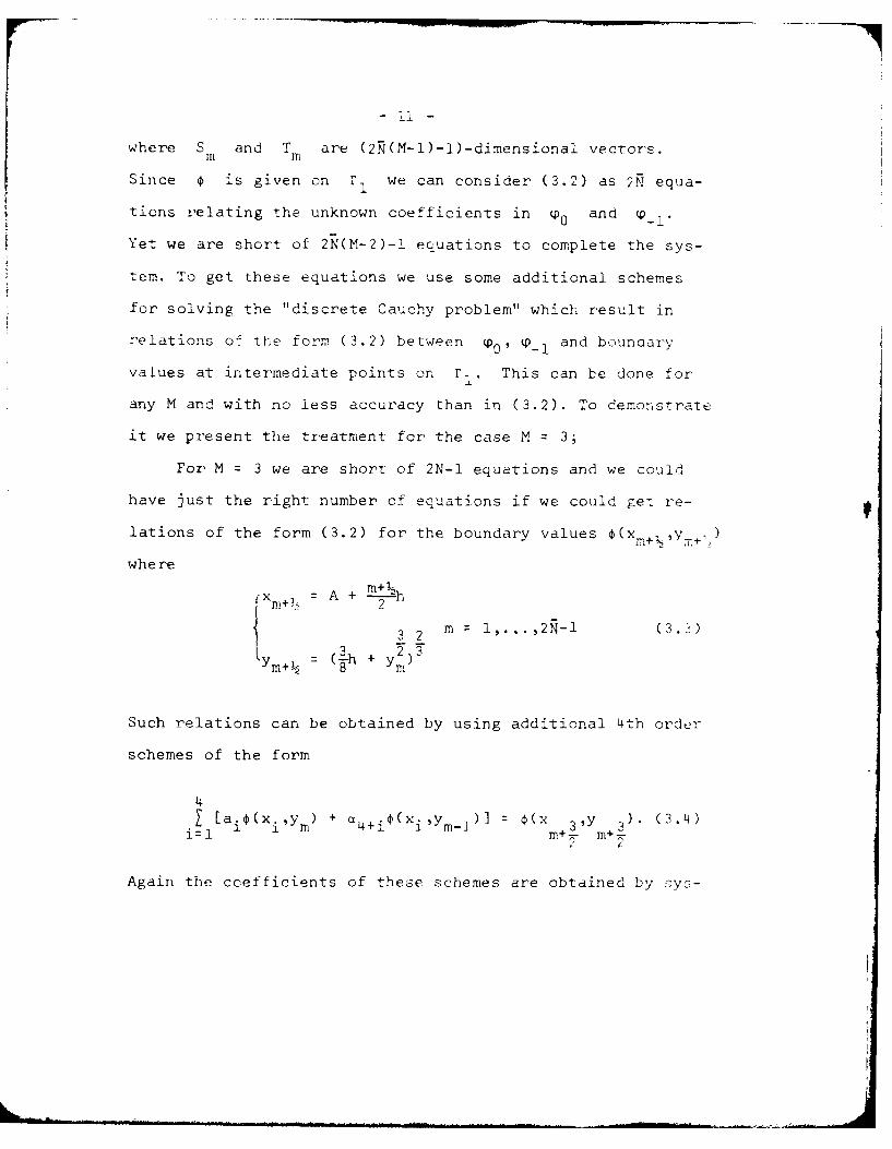
- ii -

where S and T are (2N(M-l)-l)-dimensional vectors.iii m

Since is given on rI we can consider (3.2) as 2N equa-

tions relating the unknown coefficients in 0 and 0_

Yet we are short of 2N(M-2)-l equations to complete the sys-

tem. To get these equations we use some additional schemes

for solving the "discrete Cauchy problem" which result in

relations of the form (3.2) between p0, (-l and bouncary

values at intermediate points on F1. This can be done for

any M and with no less accuracy than in (3.2). To demonstrate

it we present the treatment for the case M = 3;

For M z 3 we are short of 2N-1 equations and we could

have just the right number of equations if we could get re-

lations of the form (3.2) for the boundary values (xM+ ,y. )

where

(X=+ A +

3 2 m = i,..,2N-l (3.3)

"Y3+ (1h + y2 )3

Such relations can be obtained by using additional 4th order

schemes of the form

4[ [ai(xi,y M ) + a 4+i(x.,ym)] 4(x 3,y 3). (3.4)

i - m+T fi+ 7

Again the coefficients of these schemes are obtained by sys-

tems of equations of the form (2.5) and here we could make

the schemes be accurate for P,...,P"

In the end we have the 2N(M-l)-l relations

nh, y T + TT I - n = o ..,4N, (3.5)2 T 2

where S and T are given (2N(M-l)-l)-dimensional vectors.n n

These 4N-1 relations (for M = 3) are combined with the ordinary

scheme for the internal points in D to give a full system cf

equations for all the unknowns in D and on the parabolic line

y = 0. After solving this system we can use the vectors S and

Tn n = 2,... ,4N to produce an approximation at all the mesh points

in D+ .

- 13 -

4. Numerical experiments

In this section we present some numerical results c

applying the new schemes for several Tricomi problems. e

used the presented schemes (with M = 3) in the hyperLolic

domain combined with a simple 5 and 9-point formula in the

elliptic domain. The 9-point formula is also obtained by a

procedure of the type (2.5), i.e., by demanding that the

scheme is accurate for polynomial solutions of the Tricomi

equation. In that way we obtain a local o(6 4 ) scheme in 1-

which, experimentally, proved to be a global 0(6 4 ) where a

square mesh of size 6 is use- ir, D- In order to match theh

hyperbolic and elliptic schemes we chose 6=

We consider boundary conditions given on the lire-:

{x 11, -l Z y " } and {y = -1, -i :r x 1} in

elliptic domain and on the characteristic line

3 22 T3F, 7 {x - yv -1, 0 y . (-) } in the hyperbolic

Such conditions define a unique solution in the domain toundep!

hy the above lines and by the characteristic

3

The computat-ional aspects of the method and some additicni:

numer ical results are to be described in a separate ,.

- 14 -

Table 3. 1

Maximum error, in D = D+ U D- for the Tricomi problem

with the values of the analytic solution (2.10) of the Tri-

comi equation as boundary values on F1 U F . A scheme with

M = 3 is used in the hyperbolic domain and 5 and 9-point

formula are used in the elliptic domain.

Ax = A y :T78 -

5-point formula 0.47E-2 0.14E-2 0. 3717-3

9-point formula 0. 44E-3 0.59E-4 0. &-.

References

1. Filipov, A.F., On the difference method for solving vhe

Tricomi problem, Prikladnaya Mathematika i Mehanika, 21,

73-56 (297).

2. Guderly, G. and Yoshihara, H., The flow over a wedge pro-

file at Mach number 1, Journal of the Aeronautical Sciences,

17, 723-735 (1950).

3. Lev-1n, D., Accurate difference schemes for the solution

of Tricomi's equation in the hyperbolic region, Scienti-

fic Report, Grant No. AFOSP-77-3345, July 1979 pp. 50-7C.

4. Loinger, f., Difference Schemes for the Solution of

Tricomi's equation in a mixed region, this report.

5. Ovsiannikov, LV., Concerning the Tricomi problem for one

class of generalized solutions of Euler-Darboux equati n,

Doklady, 91, 457°,i460 (1953).

6. Tricomi, F., Sulle equazioni lineari alle derivate

parziali di secondo ordini, di tipo misto, Rendiconti,

Atti delil' Accademia Nazionale dei lincei, Series 5, 1,

134-247, (1923).

7. Vincenti. W.G. and Wagoner, C.B., Transonic flow past

a finite wedge profile with detached bow wave-general

analytic method and final calculated results, NACA Tech-

nical Note No. 2339. (1951).

V. DIFFERENCE SCHF-AS FOR THE SCIJTION

0} T I -1[lfTil. 1.11 V? PVD KEc '

FriedaI oinger

Abstract

The Tricomi problem in a mixed region is solved via a

numerical projection of the hyperbolic boundary conditions

onto the parabolic line, thus coupling the two regions. Differ-

ence schemes, exact for polynomials up to a certain degree,

are used; high accuracy is achieved in all the examples co::qpu-

ted.

1. Tntroduction

Tricomi's equation:

Y : x -P yy

i : elliptic for y < 0, parabolic for y 0 and hyperbolic for y > 0.

We look for a solution in a mixed domain D = D_ U D+ where D_ is

an elliptic rectangle bounded by x = -1, y = -1, x = +1, y = 0 and

D+ the hyperbolic curved triangle bounded by y = 0 and the two

characteristics 1'1 and F,:

2 3/2

2 3/2£2: i l =x +-y 0 x

The problem is assume well-posed with appropriate boundary con-

ditions given on x -1, y -1, x +1 and one of the character-

istics, say rI .

-2-

2. Notation

For the numerical solution of the problem we divide the region

into the following elements (see figure 1): rectangles in the ellip-

tic domain along the lines x = const, y = const and isoparametric

triangular elements in the hyperbolic domain, with the following

enumeration:

j - the no. of the row

j : - M, - + ... ,0,1 .... N

j < 0 elliptic region

j = 0 parabolic line

j > 0 hyperbolic region

is a mesh point

no. of points on the parabolic line : 2N + 1

n. - the no. of points in the j-th-row]

xi+ 1 - x i = Ax 1/N Vi in the grid

Yj+I - yj = Ay 1/M for j < 0

Yj+I - yj Ayj = (l.SAx(j+l)) 2 / 3 - (l.56x.j) 2 / 3 for

j 0

mesh points in the elliptic part including the parabolic line:

-3-

(xiY j) i= -N, -N + l,... ,O,l,... ,N ; j :-N,...,O

x ii :y +a yjj

X. - 1x y. - Ay

mesh point in the hyperbolic part:

(x. ..y.) j 1,2,...,N ; i -N,...,N - 2j

yj = (1.5Axj) ; x j (i.+j)Ax

and the numerical solution at the j-th-row:

( ) (xi j,y.) ij -N, -N + 1,...,n.

" I I . .. . ... . .... . . . ..... . .. . .. .. .. . .. ...-. .. . . .. . .. . ...2a n .. ..2 i

3. Projection of the boundary condition along F, on the para-

bolic line

The hyperbolic problem with either Goursat conditions ('p given

on I and y = 0) or Cauchy conditions (.p and (Py given on y 0) is

treated in [1] (D. Levin) using high accuracy difference schemes.

The difference scheme for (xi, yj+ 1 ) is based on the values of

o,( y at the points (x. + Ax, y.), (xi,y j ) when Cauchy conditions

are given (figure 2).

The coefficients are determined by the demand that the scheme

is accurate for 6 polynomial solutions of the Tricomi equation:

2 3 3 3l,x,y,xy,3x + y ,x + xy . Numerical experiments showed that

the schemes obtained are accurate for 3 basic functions:

2 3 3 3 2 y4 3 4lx,y,xy,3x + y ,x + xy ,6x y + y ,2x y + xy

We now look for a solution in the mixed region.

An analytic connection between the boundary conditions on T and

the )arabolic line is known:

Bitsadze [2]:

I(x) O(x,0) 1 5/6 d _ (t/2)=x d- I 2/3 i/K (t

2 y., O t (x-t)

+ Y x -(t) dtS (x 1/3

-5-

where v(x) = y(X,O)

(x,O) = o(x,y(x)) on

The connection on the parabolic line enables one to find the

solution of Tricomi's equation in the elliptic region and then

in the hyperbolic problem can be solved with either as a Goursat

or a Cauchy boundary conditions.

This report presents a numerical process for finding a con-

nection between thb hyperbolic and elliptic region, wiv nout ising

P (see also [3]). Alternatively, we look for a connectionJ

(0) (-l)between the values on F and (p , -l

Assuming the elliptic problem already solved, i.e.

(pJ) J)'...' Ni(j) ), j = -M,...,C, known, where (0) is the

solution on the parabolic line. We proceed from row (j) to

(j + 1) (j > 1) by choosing 6 basic functions as before (in the

Cauchy problem), but instead of using values of (p,py on y = yj as

it is done in [11 for the Cauchy problem we take an additional row

Y -i and the difference scheme will be based on the values of

(p at the points (figure 3): (xiYj+) ; (x i AX,y.),(xiy.)

(x -+Ax,y.1 ),(x ,yj 1 )

and we require that the difference scheme is exact for, the 6 basic

functions. Numerical experiments show that- these 7-part differ-

ence scheme using 6 basic functions are exact for 8 polynomials.

Note: if j = 0, yj = 0, yj- - Ay, i.e. the first row of the

elliptic region is taken.

The difference scheme can be expressed by

3k tQ )(x ,yj) + s 90(xkYj_l) = 0(x(xyj+ I )

xz = x . + (k-l)Ax i -N,...,n.

The coefficients (t ,sk) (k = 1,3) do not depend on x, but do de-

pend on y. In matrix form

(i+l) = T(j+I) (j) + S(i+l) ( j - ) j

whereT t t 3

2 3

j = 0,...,N- t t 3

0

T of order: nj 1 xn

-7-

0 SI S2 S

S~ j l 0 0 SIs °2 $ 3

j= 1,...,N-1

S~ j~ l ) of order nj+ I x nj_l

S2 S2 S3

-(i) SI S 2 0

S I S

Q S

\, j

Suppose we found B(J) and A such that

(J) B (0) + A( j (- I )

where

B ( j ) : n. x (2N+l)

]A j ) : . x (214+1)

B T A

B ( 0 ) I A ( 0 ) 0

then:

T+- 8 -

, - ,( ] (r ) . ( ) ( - ) + : ',+ ( - ) ( ) ('-pi ) (-

•.p('+A - .-

where:+ -

-++ A

( )

oJ o e ( C) d ( 0 ),je gel c"~ U- ,. e [ .:a ', : :,n, - . lonsr: .w :'.z . .

'JjE

. ~ ~ ~ ~ ~ ~ , :, ,., : . .. .) & e t e F:s +

r k" , . (7: t e

,N&t N ; -< ] .: .. : e : ,. C 4, . , ' -., : ; ' i 'e . -e i t o

-9 -

The coefficients of the scheme are (btained Ly t'.e demand that

it i-. accurate for 8-polynomial lead. Since the 7-point formula is

accurate for 8 polynomials the order of accuracy is not changed.

The 9-point scheme can be expressed as:

(j+3/2) =T(j+3/2) ((j) + S(j+3/2) (j-l)

where:

^(j+3/2)T ~~ n j + 3/2 x nj

a(j+3/2)S: n j+3/2 x n _,

s(J) and p(j-1) can be substituted from the equation obtained by

the 7-point formula:

(j) = B(j) (0) + A (j)

j + 3/2)T (J+3/2) (B (J) (0) +A (J) (-I))+s (j+3/2) (B (J-1) (0)

(0) ((1)3 (

P(+A( ) (0)+ ( -l)

where:

- 10 -

(j+3/2) T }(j+3/2 )B(j) + S(j+3/2)B(j-1)

A(j T (j+= 3/2)A(j) + S(j+3/2)A(J-1)

We now have 2N-1 equations for the 2N-1 unknowns on the para-

bolic line:

g.= (i) (1)=B (J) (1)(P(0) +A(J) (1 )(P(-I)

where B(J)(1), A(J)(1), B(J+/ 2)(1), A((1)

are the first rows of B AA respectively

The projection on the parabolic line can be written in matrix form:

B (0) +A (- )=

The projection matrices A and B, of order (2N+l)x(21;+l) are:

- ii -

1 0 0 10 0

() ) A(2 ) (1)

B(5/2)(1) (5/2) (1)

B(Ni)(1) A(NI)(1)N(51 ) A(5)1)

B (N- )(1 A(-1

B N 1

......... 0 1j 0 .. ....... .

4. Solution of the elliptic pr Liem

In the elliptic regio.n v: ---e ei: a :'-polnt (I) or a 9-point

difference scheme.

I)Ay p Q x v ~ , + Px, y-,y

, px ~+xy - lls(x,v) + (,(X-:,x,Y)

(- + 11P -

The 5-point difference scheme for the Tricomi ecuaticn ;oX-q-

for the point (i,j) is:

y (P,+1 2Q i. + Q~ 9- (wP i - + pz

where:

y/ jtA1/ M + 1 , -'. + 2, I

'-hi scheme is accurate fcor: x , y ,xy ,3xL + v

1) We b)uilA a 3-jin diference scheme by taking the I list

po)-lynomials which solv.e riois eqliation, i ..

I

- 13 -

2 3 2 4 3l,x,y,xyJx + /, "'+x, 56x y + y ,2x y + xy4

The demand that the difference scheme based on the points:

(x. + Ax,y. y) (x. ± Ax,y.) , (x.,y + Av) and (x,,y,)1. -1 ] ] ,

be accurate for those functions leads to a dependent system of

equations. Therefore one polynomial has to be exchanged with oo

with a higher degree.

An independent set of functions are:

2 3 y 3 2 4 3 4 4

lyxy,3x + y ,x +xy ,6x y + y,2x y + xy ,15x + 3x + 2%

The scheme is accurate for P as well, hence it is accurate for

9 functions.

Both types of the difference schemes give a system of equaticns

which is triangular in blocks:

A(-M+I) B(-M + ] ) C(-+l) l(-p+1)

(-M+ 2 (-M+2(

A B C -

A B ( 0) (0) (0)

A

- 14 -

with all the blocks having the same size: (2N+l) x (2N+l)

(-M)B = I

c(-M) 0

A(J) B(J) (J)A , B -M+1 . j . 1, are matrices of either the

5-point or 9-point difference schemes including identity equa-

tions for the boundary points (-l,jAy), (+l,jAy).A ( 0 ) and

B( 0 ) are the projection matrices (section 3), f(-M) is the

boundary condition on y = -,and f () (1) and f(J) (2N+l) are

the boundary conditions on x = -1 and x = +1, accordingly.

f (J)(1) = (P(-l,jAy)

f(J)(2N+l) = (+l,jAy) -M + 1 < j 1

fJ(i) = 0, 2 i .< 2N

f (0 g - vecter of solution on r 1.

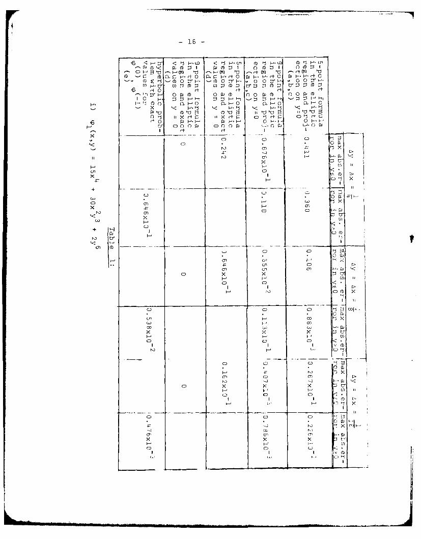
5. Numerical results

The mixed problem is solved in steps:

(0) (0)a) Computation of the projection matrices A and B

b) Solution of the elliptic problem with A (0) ( - ) + B (0) ')O g

as boundary condition on y z q.

(0)c) Solution of the hyperbolic problem using the results of p0

and (P(- I ) from (), anic proceeding with the 7-point formuia:

To see the influence of the projection condition on y = 0 the ellip-

t7c probltm is also solved with exact boundary conditions on yLQ,

.e. A = 0, B(0 ) = i and f(0) = P(x,0) i substituted in the

system (d); the hyperbolic problem is also solved with exact val-(0) (-1)

ues for ( and p . (e)

The folloiwng 3 examples are considered:

i) 1 (x,y) = 15x4 + 30x2y

3 + 2yW

Note: For this function the 3-point formula in the elliptic

region is exact.

4 2 4 7ii) w2 (x,y) -21x y - 21x y - y

fl+iiii) ?P(x,y) 2 coshx(y + 0 (3n+l)3n(3n-2)( n-...L..

n- n-1

-16 -

6~ ~ H.~ <c.O nCY

CD F- d-HO :1 -'Hq tK oq llj r- qrt OQ 'd(D r-U H- Z rt 0 L - j-r+O0 PI~..P-rt R bH P-rt 0

6 t 0 tO c-f r- . c-ft~ ojC w m 0 i D n o w (D 0 0pJ(m

(0 H a 0~H CILH 0 0j--- 0i-~i

Hrj cj0p 0 -F- 0 P O . l-

-~I c-f c-f

x 'Ati

CDD

CC

CD CD C

CD

I-D (D

Ci (P CD >-IJ '

x- In I I

C C

CD N.(D x

w C

CD C)

CD C) C)

CD x

CD CD C

CD CD CD

CT D

I , I 3>

(D CD CD

$7 Nv

((3 H H- -r_ x x x

(NCt' (.0(.0 X 1 c')r i GO

a4 ) H a)

C CD C) CDtir- U) HH

<3CC) H-

Ci C C:) C3

~C) (NA

>d. C0 (C) (N

HU) r-4 (N

r -i c(2) 1110 al H (N

4CD Hi HN H

CD0 C(0: C)

I- +- -xc H

WA L '

(dO W 0

C:) 1 H H:

C D C

CD >I ~ - ~x

C2 (14rd.( 1111-r xd uc rd-(N

Io 0 O H H C d H H04')(It 4 4 C ) 214 i 2 - X 2 - I

xOW11 CD

rd- n CD* '. 4'l

47 4J

ro ro u u D ro (_) ) 'f

WA I>) CD CD C)

a 5: x x

CD C:; C)

x ,CD cm CYD Lf<' WVi I I I

>1 CD C) CD C:)if C/) ,-4'r'- -1

Xx(0r~.HC Co) CD a)

C-) ~ -4 -rz 0

F-: C: C) C:)

WA>) C) C) C)

Ln LOCC) co C)

4 CD C:) C)

I/ I coI

CD CD (D CD-4-- '-1

<'- c-: 1'(

CD C C; C) C D~

WA I IC->) CD CD CD

x x x+

X -4 QD~CxDC CD

~.CD C.j(~ N

> C) CD CD1-4 l'-4

x cnC) CD Cfl-

CD CdU Du CD I (CD

-1- 0I Io 4-' -' r

0 -A C) 0H 0- 0H' -1 0-i T! 0 --

4 -J C)4- 4-4 P- -1l C-

o ) no' *A Q) (T0'' i *A ) (1)-- (1 4-' 0HD~ )4~ A~

r- -)

-L

- 19 -

Conclusions

The order of convergence of the 5-point formula alorn( is

O(Ax 2 ) and the order of convergence of the 9-point formula alone

is O(AX 4 ) (see results (d), table 1-3). The results of (e) show3

that the order of convergence in the hyperbolic region is O(Lx ),

approximately:

O(Ax 3 + 2 / 3 O( x 3 .Ay.) (j>O)

(estimate of error, see [3]).

The schemes used in the hyperbolic region are more accurate thar.

the 5-point formula and less accurate than the 9-point formula,

used in the elliptic region. Therefore, when the mixed problem is

solved with the projection, the maximal absolute error is obtained

in y U C in case of the 5-point scheme and the order of con-

vergence is O(Ax 2 ) in the whole region, and the maximal absolute

error is achieved in y>O when we use the 9-point scheme in the

elliptic region and the order of convergence LsO(Ax Ay.) (]>0)9

- 20 -

Ay-

Fi gu r e1

(x ,y

- 21-

/ ,//A,/

-. -L.~ 1 -f >:i/y

y.j

Yj -1x. Ax x. .+ x1

1

F _ I u a 3 F i g u r e 4

i -.2 ,j+7 j ,+ I i+ ,j+ l

A VI,

£:+

- 22 -

References:

[1] Levin, D., Accurate difference schemes for the solution

of Tricomi's equation in the hyperbolic region,

Tel-Aviv University (1979).

[2] Bitsadze,A.V., Equations of the mixed type,

The MacMillan Company, New York (1964), pp. 7E.

[3] Levin, D., Finite difference approximations for the solution

of the Tricomi equation in a mdxed elliptic-hy-

perbolic region, 1980.

Acknowledgement

The help of Yael Fried in a most competent, prompt typing

is gratefully acknowledged. For meticulous programming, and

innumerable helpful mathematical suggestions, checks and

improvements thanks go to Mrs. Frieda Loinger. Valuable informa-

tion obtained from Prof. John Osborn of the University of Mary-

land is acknowledged with thanks.