AD-AO92 634 STANFORD UNIV CA DEPT OF STATISTICS F/6 12/1REPEATED LIKELHOOD RATIO TESTS FOR CURVED EXPONENTIAL FAILITE-ETC(U)SEP 80 S P LALLEY N0001I-77-C-0306

UNCLASSIFIED TR-10 N

END

11111 .02.0

1.8

l 25i-- 1.61

MICROCOPY RtSOLUTION TEST CHARTNATIONAL RUREAUI Of STANDARDS 19(,3 A

@LEVEL

REPEATED LIKELIHOOD RATIO TESTS

FOR CURVED EXPONENTIAL FAMILIES

BY

STEVEN PAUL LALLEY

3TECHNICAL REPORT NO. 10

SEPTEMBER 1, 1980

PREPARED UNDER CONTRACT

N00014-77-C-0306 (NR-042-373)

OFFICE OF NAVAL RESEARCH

DTICSELECTEDEC 9

DEPARTMENT OF STATISTICS BSTANFORD UNIVERSITY

STANFORD, CALI FORN IA

DISTRIBUTI oN STATEMENT A

AppJoved fot public release;0 Distzibutiou Unlimited

8 0 123 0'3 1)13

REPEATED LIKELIHOOD RATIO TESTSFOR CURVED EXPONENTIAL FAMILIES

by

Steven Paul Lalley

TECHNICAL REPORT NO. 10

September 1, 1980

Prepared under Contract

N00014-77-C-0306 (NR-042-373)

for the Office of Naval Research

Reproduction in whole or in part is permittedfor any purpose of the United States Government.

DEPARTMENT OF STATISTICS

STANFORD UNIVERSITY

STANFORD, CALIFORNIA

:-- . . . ...... . , O / ,__ . . .:," " 'i m ' I .... ' '

REPEATED LIKELIHOOD RATIO TESTSFOR CURVED EXPONENTIAL FAMILIES

Steven Paul Lalley, Ph.D.Stanford University, 1980

A class of repeated significance tests for curved hypotheses

in multiparameter exponential families is studied, and asymptotic

formulae for the significance levels of such tests are obtained.

Special attention is given the important case of comparing Bernoulli

success probabilities.I--

Acf-;1on For

, hTT .. , - -

Hy_Di5stribut iozn/AvO1It~billty Cod..s

vi

1t

ACKNOWLEDGMENTS

Professor David Siegmund has been a constant source of

encouragement, ideas, problems, and advice in my years at Stanford.

For all his help, and all I have learned from him, I am most

grateful.

Throughout the past year I have had enlightening conversa-

tions with many people concerning subjects related to this work: I

would particularly like to thank Robert Berk, T. L. Lai, and Michael

Woodroofe.

I am indebted to Wanda Miller for her patience in typing the

manuscript, and to Mike Steele and Brad Efron for reading it.

nib

TABLE OF CONTENTS

Chapter Page

1. Introduction ........ ............. 1

2. Example: Testing for the Equality of Two Bernoulli

Parameters ...... ..... ...... ..... 3

3. Preliminaries Concerning Exponential Families and

Statement of the Main Result .... ...... 15

4. Normal Approximation in Several Dimensions ...... 30

5. Expansion of Likelihood Functions ... ...... 37

6. The Collapsing Argument ....... .... 45

7. Proof of Theorem 2 ....... ......... 54

REFERENCES ............... ..... . 61

iii

REPEATED LIKELIHOOD RATIO TESTSFOR CURVED EXPONENTIAL FAMILIES

1. Introduction

We study here the significance levels of repeated likelihood

ratio tests for nested hypotheses in multiparameter exponential

families. In various hypothesis testing situations, the peculiar

constraints of medical research (and the even more peculiar con-

straints of non-medical research) occasionally preclude the determin-

ation of a sample size in advance of experimental results: various

authors (notably Armitage [i], [21, and Schwartz [11]) have argued

that in many such cases a reasonable option is provided by certain

simple stopping rules based on the behavior of a (generalized) like-

lihood ratio statistic. Unfortunately, determining the operating

characteristics of such procedures remains a difficult issue,

although in recent years important advances have been made by

Woodroofe [14], [15], [16], Siegmund [121, and Lai & Siegmund [91,

[10].

Let {P, e cfl} be an exponential family of probability

measures on MP:

(1.1) (dP 0/dPO)(x) - exp{e Tx _41(0)}

The natural parameter space fl is assumed to be an open subset of IR

P

and * is assumed to be strictly convex on fn. Suppose that " is a

smooth relatively closed ql-dimensional submanifold of n, and that

00 is a smooth relatively closed q0-dimensional submanifold of n 1,

where 0 < q0 < q, < p: these are to be the null and alternative

hypotheses, respectively. (In the terminology of Efron [5],

(PO 8 C i ) are "curved exponential families.") Let X,,X 2 , ... beAn

i.i.d. from P0. and let e be the generalized likelihood ratio sta-

tistic for testing

H 0 : eS v. H : EI0 01 1

The repeated likelihood ratio test will be based on the stopping rule

T A mi , where

(1.2) T -T min{n>m0 : A >a)a-0 n

if T < ml, H0 should be rejected, whereas if T > ml, H0 should not be

rejected.

The main result of this work is that for m- -1~ 1 a , and 80 E 0

(1.3) P8 0{Ta < ml) - C a (qe-q0)/2 a

as a , provided a certain host of regularity conditions are

satisfied. The constant C, which depends on 0O, E,, and E2, will

take the unpleasant form of a surface integral in ]Rp , which may,

however, be evaluated numerically in many cases of statistical

interest.

2

-....--.,: " ., . . .. . ..-. .. . . ,

2. Example: Testing for the Equality of Two Bernoulli Parameters

Suppose we observe a sequence {(XiYi) :i -1,2,... 1 of

i.i.d. random vectors taking values in the set (0,112 with

e e (1-e1) (l-e2)(2.1) P { l.el, Y 1 e2 p1 p2 (l-pl) (l-p 2)

where el,e2 (0,11. The parameters p1 and P2 are unknown; we wish to

test the hypothesis Pl - P2.

Imagine that the variables Xi,Yi are success indicators in a

clinical trial. Patients suffering from a particular disorder arrive

infrequently at a clinic where they may be treated according to one

of two procedures: because of the nature of the disorder the

patients must be treated Immediately, and a response (success or

failure) is apparent within a relatively short period of time

(compared to interarrival times). If the disorder is serious,

sequential experimentation to compare the efficacies of the two pro-

cedures may be appropriate.

Such a situation was considered by Siegmund and Gregory [13],

who proposed several sequential procedures for testing the hypothesis

Pl " P2" One of these was a sequential version of the generalized

likelihood ratio test, which had previously been studied in different

contexts by Armitage [1], [2], Schwartz (11], Siegmund [12], and

Woodroofe [15], [16]. This test is easily described. Let

3

hE: 7

(2.2) H(x) - x log x + (1 -x)log(l -x)

I(x,y) - H(x) + H(y) - 2H((x +y)12)

A n I(x,y n )n U

T-T =min(n>m *A >a}a 0 n

where

-n-- -1 nx n n E XiXn j pI

nyn = n- E Yj •j=l

The variable A is the logarithm of the generalized likelihood ration

statistic, which is commonly employed as a test statistic in fixed

sample procedures. In using it as the basis for a sequential test,

one observes pairs (Xi,Yi) until the time T A m1 (m1 being some fixed

patient horizon), rejecting the hypothesis P1 f P2 iff T <

The problem of computing significance levels and power func-

tions for the test procedure just described is not nearly so easy as

for the fixed-sample generalized likelihood ratio test, whose asymp-

totic theory has been thoroughly developed. Siegmund and Gregory

(131 have derived heuristically an asymptotic formula for the Type I

error probability; their formula agrees formally with a result of

Woodroofe [151 which was proved under assumptions too stringent to

include this problem as an admissible case. This formula is con-

tained in Theorem 1 below.

4

THEOREM 1. Let E, and E2 be fixed constants such that

(21og2) El < E . Suppose that mO = aEi + o(a) and

= aE + o(a) (recall that Ta = min{n >m : A >a}). Then as a :

(2.3) a- 1 /2 ea Ppp {Ta<mi} - C(p;E,E)

for every pE(O,l). For 0 < p <1/ 2 , C(p;j, 2 ) - C(2p-1/2; El,E)

and

(2.4) C(p; E,E2)

7T-1/2 V(,2p - )[I(,2p -)]-1/2

lc(0,2p) n {:E21 <I(E,2p-C)<E } I

[p(l-p)/E(l C)(2p )(I+C 2p)]I1/2 dE i

and

-(AT-a)(2.5) v(plP2) f lrm E e

a- op2 Plop2a-' 2

That the limit in (2.5) exists (except for a countable set of

for which p1 , P2) is a consequence of Theorem 1 of Lai and

Siegmund [9]. In fact, Woodroofe [161 has obtained an integral

formula for the function V(pl,p2) which is explicit enough to allow

numerical integration.

The restriction on the initial sample size m 0 is rather

peculiar and deserves some comment. Notice that the function

2I(Pl,p 2) is bounded for (plP 2) C [0,11 : it achieves a maximum of

2 log 2 at the points (0,1) and (1,0). Thus A > a can occur only ifn

! '-' ,....Ct..,.*:, , ,

t

n > a/2 log 2. Moreover, if A > a for some n close to a/2 log 2,n

then (xY) must be close to either (0,1) or (1,0); since in most

conceivable applications neither p1 nor P2 would be close to zero or

one, it would be somewhat unsettling to terminate the experiment on

the basis of such an anomolous sample. A larger initial sample size

protects against this possibility.

In the following sections an analogue of Theorem I will be

formulated and proved under the assumption that the observations are

from a multiparameter exponential family. This theorem will have one

major shortcoming: namely, it will be necessary to impose even more

stringent requirements on the initial sample size. (For the problem

discussed in this section, the hypotheses of Theorem 2 would require

> (log 2)-1 , i.e., that the initial sample size be twice as large

as Theorem 1 requires it to be.) The mathematical difficulty which

necessitates the stronger conditions stems from the fact that large

deviations theorems need not in general be uniform near the "boundary"

of an exponential family. Fortunately, this difficulty disappears in

many concrete cases of pt ,.cal importance: for instance, whenever

the mean parameter space is all of IRP; and also in multinomial

families.

We will give a (somewhat sketchy) proof of Theorem 1 for

those cases where

(2.6) N(E,,E2 ;p) = {(r, 2p-r) :0 < r < 2p and

< I(r, 2p- r) <E1

6.9.

is contained in the open square (0,I) x (0,1). The argument has two

steps: first we show that only those sample paths for which (xT,YT)

is "near" N contribute substantially to the probability in (2.3);

then we perform a local analysis near N.

PROPOSITION 1. As a + o

-l-1/2 -k -a(2.7) Pp,p{Ta<a dist((xT,YT),N) >a log a) = o(a e

for every k > 0.

NOTE: In adapting the arguments presented here to the more general

problem discussed in the following sections the primary difficulty is

in obtaining analogues of Proposition 1 (cf. Section 6). It is

because of these difficulties that the more stringent assumptions on

initial sample size are necessary.

PROOF. This is based on the "fundamental identity of sequential

analysis," viz.,

(2.8) P ,P (A) = 'A LT dQ = 0 0 (E IA LT)dpl dp2

where

(2.9) Q(B) = i 0'O P, P2 (B)dpl dP 2

and

L p p)n(2-x-Y(2.10) L n = (n +1)2nxJ nyj

7

(Here Q (B) is defined for all events Be c ( 1 Y)(X, 2 ,. ) and

(2.8) holds for all A in the "stopped"' 0-algebra of events A such

that Anl IT nl3 (X Y),.(X ) for all n).

Stirling's formula (cf. Feller [6], Chapter II, inequality

(9.15)) provides a (crude) upper bound forL

-A(2.11) L < Cn e nen

where

(2.12) E n n[2H((x n+y n)/2) -(x n+y )log(p/(l-p)) -2log(l-p)]

for some constant C > 0. Now

H()- W~ log(p/(l- p)) - 2 log(l- p)

is a strictly convex, smooth, nonnegative function of wi E (0,1) which

is zero for wi - p and satisfies H"(w) > 0. Thus there is a constant

C*> 0 such that (x,y) E (0,1) 2 and

(2.3) dist((x,y), {(r,2p- r) :0 <r <2p}) > 6

implies

(2.14) 2H((x +y)/2) - (x-ey)log(p/(1- p)) - 2 log(1 -p) > C 62

Clearly (2.8), (2.11), and (2.14) imply that for every 6 > 0

(2.15) P PIP{Ta S 1 1; dist( (-XTIYT),{(r,2p-r):0<r<2p}) >6a_1loga}

a o(ak e- )I

for every k > 0, since A T> a.

8

*Ot Uko

Similarly it may be shown that if T < a

dist((xT,YT), N) > a - /2 log a, but

< 1a- / 2 oa

dist((xT,YT), {(r,2p -r), 0 <r <2p)) < 6a 1 log a

for some (sufficiently small) 6 > 0, then

_**

(2.16) AT -a > C log a

this together with (2.8) and (2.11) imply

(2.17) P {T <al dist((,) N) > a- 1/2 log a,

PI T~E ; TYTlga

dist(xT,YT), {(r,2p-r), 0 <r <2p}) < 6a-I /2 log a)

o(a-k e-a

for all k > 0. This and (2.15) imply (2.7). //

For the next step of the proof we will again exploit the

fundamental identity of sequential analysis, but with a new prob-

ability measure, which we will again refer to as Q. Let

(2.18) Q(B) C Pr,2p-r (B)dr/(2p)

then

((n) ,d^ (n) 2L 2pr nx n n-nxn(2p -ny(2.19) dp~pl/d n 0 r (l-r) -r)

( +r -2p) ndr/(2p)

F 9

(where P (n) and Q n denote the restrictions of P PPand Q to

PROPOSITION 2. Suppose that for some (r,2p -r) EN,

(2.20) dist((x ,yn ), (r,2p -r)) < n /

Then as n -+ W

(2.21) L -A nn a (2p)((2r(l -r)) 1l +(2(2p -r)(1 +r -2p))1)l1/2n IT

x T -r

ex {i[ Mf J

where

(2.22) (r( -r))' ((2p -r) (I+ r -2p))'

(r~ -r))-1 ((2p -r) (I +r -2p))Y-j

Relation (2.21) holds uniformly for (x nyn) satisfying (2.20) with

(r, 2p -r) E N.

The proof of this is omitted: it is a straightforward but

tedious exercise in the use of Laplace's method of asymptotic

expansion.

The strategy for the rest of the proof is to show that for

each (r,2p -r) F-N, (A T-a) and

10

.. ... ....

rT-r+r -2p

are approximately independent under E r,2pr as a + =. For then the

Central Limit Theorem, the Nonlinear Renewal Theorem of Lai and

Siegmund [9], and the fact that

T P(2.23) A r,2p-r, 1

a I(r,2p -r)

will make possible the evaluation of E a- 1/2 e-a L 1A, wherer,2p-r e T 1A'hr

(2.24) A = {T <a 21; dist((xT,YT), N) < a - I / 2 log a)

Nearly all of the technical difficulties associated with this

program are obviated by the following inequalities.

LEMMA 1. Let S have a binomial distribution BI(n,p) under

Pp, p c[0,1]. Then for each k > 0, 6 > 0, and a > 0

(2.25) max P {ISn- nP >6n log n) - o(n-k)

and

r i +a} ~ 6n(2.26) max P [ISn-nPI >£n - o(e - )

0< _ p n

PROOF. Using the Markov inequality,

II

11

........ ......................... . ......................... ., , r_, .

P (S -np< n1/2 f(n)) < E exp-8n-I/2(Sn-np)/e-f( n )

p n (- n

-e OPn 112 (1 - p +pe- n -1/2 ) n/e - 6f(n )

- exp(pnn 1/ +( 2 0)en ) O(1)/e - f(n)n

for a > 0, f(n) < 0. It is clear from the Taylor series expansion

that the 0(1) term is uniform in p. The reverse inequality may be

obtained similarly. //

COROLLARY 1. As a o

,1/4

(2.27) max P {T a [n2, n} =o(e -a )(r,2p-r)cN r,2p-r

(2.28) max P(Ln- , C/log a,(r, 2p-r)N r,2p-r n n

1/16some n ,in2,n3 ]) = o( - a )

(2.29) max P xy >Ca- 1 12 log a)

(r,2p-r) r,2p-r n n Yn -1/

1/32o(e-a

here

(2.30) n nl(a,r) - [a/I(r,2p-r) -a + °

(2.31) n2 = n2 (a,r) = [ a/I(r,2p - r) -a +j/2

(2.32) n 3 = n 3 (a,r) = t a/I(r,2p - r) +a +tn/2

12

S. .... .... ....... . ..

(2.34) (r) n

n n-n+ 2pI r Y +r - 2pj

and n c (0,1/32) is some fixed constant. Relations (2.28) and (2.29)

hold for all C > 0.

The corollary is an easy consequence of the preceding lema.

Define

(2.35) A -Anf {T c nn1r a [n 2 ,n 3 ]}

n T - nl (r) l/log a)

n {ilx r - x j+ 1Y - I < a'.1.2 log a)

nl {x -rI +1Y +r-2pl < a

by Proposition 2

(2.36) 1A a-1/2 ea LT - 0 (eClog 2 a)

for some C > 0, so the Corollary implies that

/2 eaP -1/2 ea LT)dr/2p(2.37) a- ea Pp,p (A) = Er,2p-r (A T

f pE a- 1 2 ea LT)dr/2p +o(l)r

Now by Proposition 2 and (2.35),

13

. - ..............................

-12- (AT-a) 1 r)1/2(2.38) 1 a- 1/ 2 ea L e (- I(r,2p- (2p)

A T , 7)) (pr

(2r(l-r)-1 + (2(2p-r)(l+r-2p))-l)1/2

exp{fnl(r)/2}lAr

and this hold uniformly for r £N on A .r

The "asymptotic independence" argument is completed by the

following result.

PROPOSITION 3. For each r cN such that the random variable

I(r,2p-r) + (XI-r) I/ p l l(r,2p-r) + (YI +r- 2 p)MI/ p2 1(r,2p-r)

has a nonlattice distribution when Y - Pr,2p-r'

(2.39) E r,2pr[e I ] - v(r,2p- r) Pr,2p-r.

This result is implicit in the proof of the Nonlinear Renewal

Theorem given by Lai and Siegmund [9].

It is relatively easy to deduce Theorem 1 from (2.37)-(2.39).

Uniform integrability problems may be handled by using (2.36), the

Lemma, the Corollary, and the Berry-Esseen Theorem (for random

vectors). The details of these arguments are straightforward but

tedious, and will be omitted: they would, perhaps, serve only to

obscure the basic argument. The bloodthirsty reader should rest

assured that his appetite for raw, gory arguments (and detailed

obscurity) will almost certainly be satisfied by the end of this

work.

14

;~ ~ ~ ag .- --i-- ..- -

7f3. Preliminaries Concerning Exponential Families

and Statement of the Main Result

Let Xl1 X2,... be an i.i.d. sequence of random vectors each

with law P We will not distinguish between PV, the measure on Utp ,

and P8, the measure on the a-algebra J(XI,X 2,... ). Recall that if

X - PV' then

(3.1) E0 X V e(0 i!

cov e () - ( ; Le

since we have assumed * to be strictly convex, (O) is perforce

positive definite for each e £!. Assume that vi - 0.

Let r - e;2l} be the mean parameter space. Because

$() - (0) is strictly positive definite, the map

(3.2) f2 : r by

e p

is a diffeomorphism (this is the Inverse Function Theorem of

Calculus). Thus although r need not be convex, it is an open subset

of IRP.

The (nonnegative) function

(3.3) O(x) - sup ( Tx-(8))eCQ

is the "convex dual" of *. For x cr the supremum in (3.3) is

uniquely attained at that 8 for which V - x; henceforth this 8 will

be referred to as O(x). It is evident that for x cr

15

(3.4) V 0(x) - 0(x)

x

V2 *(x) -4(0(x)f1,

Moreover, since 0 cl (by (1.1)), the set

(3.5) Kb = fx IRp : 0(x) < b)

is compact for each b > 0.

Recall that QI is a smooth, relatively closed ql-dimensional

submanifold of Q and QO is a smooth relatively closed qo-dimensional0

submanifold of SI" Since 0 - P is a diffeomorphism, ri = :66i i

are smooth relatively closed submanifolds of r. (NOTE: A convenient

and elementary source of information concerning the topological and

geometric concepts used here is Guillemin and Pollack [81.) Define

convex functions 0 and 01 by

(3.6) 4i(x) - sup (aTx -( 6 ))

the log generalized likelihood ratio statistic is then

(3.7) A = n( (S n/n) - 00 (Sn/n))

It is apparent that the behavior of the functions 0 and 01 will play

a crucial role in all that follows.

Unfortunately, for a given x r JRp the supremum in (3.6) need

not be uniquely attained. For 00 CQV a necessary condition for

(3.8) T0 x-( 0 )- sup (0 Tx-

16

is !Lisi

(3.9) x - TO0 i(60

0

where T1i(O0) is the space of tangent vectors to Si in IRp .

(Throughout the paper we will use the notation TN(y) to denote the

space of tangent vectors to N at y: i.e., if N is a q-dimensional

submanifold of ]Rp , then for y E N

(3.10) TN(y) = {v IRp : 2 smooth g :[-i,1] N

with g(O) - y and g'(0) - v}

For each y EN TN(y) is a q-dimensional vector subspace of mRP.) Let

(3.11) U, = {x Er :the supremum in (3.6) is attained uniquely

at some point i(x) E

.

LEMMA 1. For each 0 F i the affine space p 0 + Ti1(0) intersects ri

transversally at p." Furthermore, for each 6 EP there is ai

neighborhood N(p.) of Pi(open in r) such that N(p0 ) c U, and such

that

A6 1 : N(I0)

is a smooth submersion. If x sr has an open neighborhood N C Uix i

such that 0 :Nx Q i is a smooth submersion, then

(3.12) x *ix - eWX) ,

(3.13) vT V_ *i(x) v > 0 y vWTi(Bi(x))

17

--- _-

and

T V2(3.14) W~ i~). 0 C STO (8(x )

NOTE: Let N, and N be smooth submanifolds of IRP, and let12

y cNI n 2*Then N 1and N 2are said to intersect transversally at y

if the tangent spaces together span JR, i.e., if

(3.15) TN I(y) + TN 2Cy) - .

A map g : N 1 ),N 2is said to be submersive at x c N if for every

v eTN (g(x)) there exists a smooth f :[V.1,1] -4 N1 with f(O) = x such

that (g of)'(O) = v; i.e., if dg xmaps TN 1(x) onto TN 2 (g(x)).

PROOF OF THE LEMMA. Since dimO.'a +T%2 1(0)) + dim(Tr i(ii ) p, the

transversality of P+ TQ 1 (6) and r . at I.' will follow from showing

(3.16) TfQ1(0) fl Tr (PJ0 {o)

For (3.16), suppose g :-11 is a smooth map such that

g(0) - p then since V:Q~ r is a diffeomorphism, there is a

smooth f : [-1,1] SI i such that f(O) = 00and g~t) = Vi(f(t)). Now

g'(0) V= ipmfo)) - f'QJ)

t= 0 f'(0)

Since f'(0) ETS 1 (0 0 and j(0 0) is positive definite, it is impossible

for g'(0) 2i (aN 0 This proves (3.16).

18

Fix 80 £Qi there exists a neighborhood N(V8 ) in r such that

if xcN(j0e ), then

(3.17) sup{(OT x- *(8)) :O E i and 10 N(110)11 0

T< sup{( T x-*(O)) :OCR i and 1' EN(O11

and such that the supremum on LHS (3.17) is not attained. Now N(N.O) i

may be chosen small enough that the affine spaces pe + Trn(e) give a

"smooth fibration" of N(PO ): i.e., for each xcN(j0 ) there is a0 0

unique e for which x ell + T~i(8 x) ,and such that the map x 0x i x

xis smooth and submersive. (This fact relies on the fact that the

spaces p + TQ (O) intersect r1 transversally at p,, together with

the fact that the map 0 + TQi(6) is a smooth mapping into the set of

qi-dimensional vector subspaces of IRP.) But the necessary conditionA

(3.9) together with (3.16) implies that for x eN(1i0 ), ex =ei(x) •

Next, suppose that x er has an open neighborhood N c U suchx i

that :N R+i is a smooth submersion. Then

(Waxj) e(x) = (9/1 xj)(ai(x) Tx - (fi(x)))

- (Gi(X))j + k- [(a/axj)(oi(x))k] "xk

- z [(a/axj)(ei(X))kJ • (/lek(eix)) =- (X)k-i

since by (3.9) x - v0 (Oi(x)) ± T i(ei(x)). It now follows from

(3.12) that

19A IA

sinc by(3.) X 6 (6 W ili 0 1(x). I nowfolowsfro

(3.12 tha

(3.18) V x *(x) ((/ax)(ai(x))k)j,k-l,...,p

since x 6 ei(x) is submersive this matrix includes TRi1(e(x)) in its

A Irange, and clearly TS i(ei(x)) is contained in the kernel. Thus

V4 i(x) is invertible on TO i(i(x)). On the other hand it is non-

negative definite on IRp since 4i is convex. Consequently it must

be strictly positive definite on TQi(ai(x)). It may also be shown

using (3.18) that V" 4i(x) f T i(ix)) 0. A

Lemma I gives a partial indication of the importance of two

topological regularity properties: namely, transversality conditions

and the submersiveness of the MLE maps. Another reason the trans-

versality conditions figure in the analysis stems from the following

purely topological fact, which will be exploited in Section 6.

LEMMA 2. Suppose V is an open subset of IRp , and NI,N 2 are rela-

tively closed submanifolds of V. Let K be a compact subset of V such

that if x F N1 N 2 O1K, then N 1 and N2 meet transversally at x. Then

for any E > 0 there exist 6 > 0, 6 > 0, and a0 > 0 such that for any

a > a0 and any ycV

(3.19) dist(y, N1 n N2 n K) > E/a

dist(y, N1 OK) < 6/a

implies

(3.20) dist(y, N2) > 6 /a

20

fk.

I

In other words a point cannot be far from the intersection

without being far from one or the other of the two manifolds. This

is manifestly untrue of manifolds which intersect nontransversally:

e.g.,

I {(x,y) € :~ 2

2 2N {(xy) e]R :y=O

2

PROOF. We will give only a rough outline of the argument. Suppose

first that N and N2 are affine subspaces of MRP: the existence of

and 6 follows from the construction of disjoint angular corridors

around N1 and N2 as illustrated by Figure 3.1

.' /

, (cross section)

i/

~Figure 3.1

= 21•- ,--

,i -- ". .... . .. -

In the general case, N1 and N2 may be approximated to first

order by the appropriate translates of their tangent spaces; if N1

and N2 intersect transversally at x, then the tangent spaces TNI(x)

and TN2(x) intersect transversally. Angular corridors may then be

constructed as before. Thus for each x EN n N n K there is a1 2

closed neighborhood Ux in ]Rp and constants x' 6 , a0(x) such that

for a > aO(x) and y EV

dist(y, N1 n N2 K AU) > E/a

and

dist(y, N A K A U) < 6 /a

imply

dist(y, N2) > 6 /a

The lemma now follows from a compactness argument (since N1

and N2 are relatively closed in V and K is compact, N1 A N2 A K

is compact). ///

The conclusion of the main theorem depends heavily on the

assumption that the MLE maps behave nicely near a certain critical

manifold, and also that the manifold r not contort itself too

strenuously in certain regions of r. Let 00 CS0, and define E(60)

to be the largest extended real such that the following three condi-

tions are satisfied:

22

T

I. For every E, O<E<E 0 , the set {x r :(x)- ex+*(e 0 )< E

is compact.

II. For each xer1 0 (Wie 0+T0( O) ) such that *1(x)- o(x) <E%

there exists a neighborhood Nx of x in r such that Nx C U0

and e0 is a smooth submersion on Nx, with 6 (x) - 0.

III. For each xEr fl (' o+T0(O) ) such that W(X) - W(X) <E,1 60 ±

r 1 intersects (P 0 +T%( 0() ) transversally at x, and r 10T Tintersects the level surface fy e r :v(y) -e 0 y . (x) -60 x)

transversally at x.T

Note that there is always a positive E such that {x Er :(x) - 0 x

+ < E()< is compact, since {x ER p : 4(x)- Tx+1P(6 O)<E} is com-

pact (cf. (3.5), and reparametrize the exponential family). That

(E000) >0 may be deduced from this and Lemma 1. It should be noticed

that in the special case Q 2 1 condition III is automatically

satisfied, and in case r = iRp, condition I is automatically

satisfied.

THEOREM 2. Suppose 0 < El < 2 < %(00); recall that

1

(3.21) Ta T - min{n>a :A >a}a -- n

Then as a +

(ql-q 0 )/2 CE, 2 o(3.22) P 0 fTa<aq I a , ea C(EE; 60 )

where

23

.. .

f -(q1 -qO)/2

(3.23) C(E,E 2 ; 0 = v(y)(27r( (y) -4o(y)))

0 E( ,E2 ;00)

[det(H 2 (y))/det(t(6(y))(HI(y) +H3(y)))]1/2

a a(dy)

±

(3.24) M(E1 , E2;O) - {y C 1 (P, 0 +1T0(G0) ) E <(y) -00(y) <E

-(AT-a)

(3.25) v(y) = lim E^' e

a- 0y)

(3.26) H1 (y) = $(5(y))-iPH2 (y)- P (Ow(y)- 1

-1(3.27) H2(y) P T(8(y)) P (I0(00) 0 TF 1(y))

(3.28) H3(Y) =(O(y))-_V2 0y (y) +V2 0 (y)

P is the orthogonal projection operator onto the space

IV 0(0 ) n Tr1 (y), and a is the volume element measure for the

manifold-with-boundary M(EE 2 ; 0).

Many comments are in order. First, conditions I and III

(transversality) imply that M(E,E 2 ; 80) really is a compact

manifold-with-boundary: this is a consequence of the Implicit

Function Theorem. Second, the "det H2 (y)" which appears in the

numerator may be confusing: H2(y) is a (positive definite) operator

on Tr 1 (Y) n T0O0 (6 , and the determinant is simply meant to be the

product of its eigenvalues on Trl1(y) n i%(0) . Third, it remains

24

Aft

to be seen that the integral is finite, and in fact that the inte-

grand is defined (cf. (3.25)). Notice that 0 is a continuous

function which is bounded away from zero on M(EE; O0). The other

two factors of importance require more care.

LEMMA 3. For every y cM(Ej,E; 0 ) the matrix H (y) + Hs(Y) is

strictly positive definite on IRp .

PROOF. Since s(e) is everywhere strictly P.D. it is clear that H (Y)

is N.N.D. on Rp and strictly P.D. on TQ0(0) - n TrI(y). Also if

y EM(EIE 2 ; 00), then since E < V0) and Ye0) satisfies

condition II, it follows from Lemma 1 that V2 40 (y) is N.N.D. on 1Rp

and strictly P.D. on TQ (6

Now consider 7 2( - 1 )(y). Since - is a nonnegative

function on IRp which is zero on rl, V2(0- 1 )(y) is N.N.D. on IRp

whenever y crl, by Taylor's Theorem. Furthermore, if yc rI , then

y (y) is zero on the vector subspace TI(0(y)) (cf. (3.14) of

Lemma 1). Thus V(o- )(y) is strictly P.D. on T (6(y)) for eachS I-

y cr I. Now since (y+In1 (O(y)) ) intersects r1 transversally at y

(Lemma I again) it follows that Vy( - )(y) is strictly P.D. on

y 1

Tr1 (y).I I

But TrI(Y) + in 0 (e 0 ) +(I0 (e) n Tr1 (Y)) - fRP, so

Hl(y) +H3 (y) is strictly P.D. on TRp . I/f

As for v(y), the existence of the limit in (3.25) is a conse-

quence of a general theorem of Lai and Siegmund [9]. In order that

their theorem be applicable, however, a certain random walk

25

associated with the process [A n must be nonlattice. In the next

le-a it is shown that this is so far almost every y cM(E,,E 2; Vo)

LEMMA 4. For all Ei< < E(

(3.29) afy cM(E 1 , E2 ; 80) 01)- ()+ X-y)T70 ))

has a nonlattice distribution when X 1 P 'y I = 0

where y(-) denotes the volume element measure on M(E ,E; 10).

PROOF. Call a point w c IRP a support point of the exponential family

if for some 0 c S1 P fu u -. iw < E) > 0 for each E > 0. Clearly if wi is

a support point, then P0*fu: u - w < E > 0 for every * c S and E >0.

Because the covariance matrices t(O) are strictly P.D., there exist

support points U11,* .. ,90u which form a (vector space) basis for IRP.

Let

=(Y 1(y) - 0(Y) ,ye 1R

A necessary condition for I(y) + (X 1 y)T V y (y) to have a lattice

distribution (under P 3(y)) is that for any pair { JiG of the atoms

there exist a rational number qj',such that eithert

(3.30) qfij (y) +(c y)TV I (y) 1(y) + .y)T V ICY)

or

YT T ~)) I

(3. 31) q j (y) +(coY Y) +~) (6 1 +CiY) Vy I()

26

Suppose that there is a y Y cM(EE; '0) such that conditions

(3.30)-(3.31) are satisfied for y - yo and some particular set

{q{jj}} of (p) rational numbers: we will show that there is a2

-'-

neighborhood N(yo) of yo such that if ycN(Yo) nlr1lnw. o+ 0 ),0

then (3.30)-(3.31) are not satisfied for y and the same set of

rationals {qfij}}. By the countability of the rationals this will

prove (27).

Suppose the indices are labelled so that alternative (3.30)

holds. Consider the first order Taylor series of

(3.32) f~ (y) fI(y)(l -qi,j})

+ (Wi-q{i,j} j- y(l-q{i,j 1 ))T VI(y)

around y y0 :

(3.33) Tf{i,j}(y) f (-q{ij} GJ Y0 (l-q{i,j}))

2 I(Y) 0 (y-yo)

Since V2 O0(yO) t 'M 0 0, Lemma 1 and the transversality

condition III imply that V l(Yo) (inO (6 TrI(yo)) is strictly

P.D. Consequently, because ... ,c is a basis for ] p , it follows

that for each uc (In0 (60 ) 0n Tr1 (y 0 )) satisfying lul 1 1, there is a

pair {i,J) such that

(3.34) Tf{i,j}(Y0 +tu) 0 0

whenever t I 0. Since Tf{ij } is the principal term in f~ij} and

27

since B fu e( UO(6) n Trl(y 0)): Jul I} is compact, there is a

6> 0 such that

f fi,j } ( y ) 0 0

for any yr I n 0 + S0 (800 satisfying 0 < ly-y01 < 6. This

proves the lemma. //

Although this lemma together with the result of Lai and

Siegmund shows that the function v(y) is well-defined for almost

every y (do), there is as yet no hope of evaluating it. However, an

important result of M. Woodroofe has v(y) expressed as an integral

involving only the characteristic function of the random variable

considered in Lemma 4. Woodroofe's theorem makes possible the evalu-

ation of the constant appearing in Theorem 2 by numerical integration

in many cases of statistical interest: his paper [16] contains not

only a proof of the theorem but several interesting examples of its

use. (NOTE: Actually Woodroofe's theorem carries certain hypotheses

concerning the smoothness of the underlying distributions which are

unnecessary, as an elementary modification of his proof shows).

Theorem 2 generalizes another theorem of Woodroofe (Theorem 3

of [15]) which essentially covers the case Q= Ql, but under smooth-

ness conditions on the distributions {P 0 which rule out all problems

involving categorical data. His proof seems to be very much tied to

these assumptions, and bears no resemblance to the approach used in

this work.

28

. . .. .... ....

For the proof of Theorem 2 we will assume that Oc Q and

8 - 0. For arbitrary 6 e% we may always reduce to this case by

reparametrizing and recentering the expoential family.

29*1 AW N -,~.

.

V

4. Normal Approximation in Several Dimensions

Certain refinements of the multidimensional Central Limit

Theorem play a key role in the analysis which follows. Of primary

importance are (1) bounds on the probability of moderate deviations

of the sample mean, and (2) uniformity in the convergence ofn-i/2Sn.n1 (S - ni0) (under P0) over compact subsets of the natural param-

eter space.

Let t be a symmetric positive definite matrix on fP, and let

Qt be the Gaussian measure on IRP with mean zero and covariance ,

i.e.,

(4.1) QVA) = (det $)-i/2 (2 ) -p/2 fA exp{-yT $_'v/2Jdy

for Borel sets A. In addition, let CU be the class of p-dimensionaln

half-spaces

(4.2) A (a) {x c IRp T x a

where

= 1

and

0 < a < n /6/log n

PROPOSITION 1. Let K be any compact subset of Q (the natural parame-

ter space of the exponential family {p0), which is assumed to be an

open set of IRP). Then

30td

(4.3) lir sup sup P -nn-1/2( 0 ) (A}/Qt(e) (A) I 1n-*- OcK AeG

n

and

(4.4) lin inf Inf P {n-1/2 (Sn-np0 E A}/Qt(0 ) (A) 1 1n4 - 0cK AeG

n

The proof of this is a rather tedious modification of the

proof of Cramer's Theorem (cf. Feller [7], Chapter XVI, Section 7).

The only real novelty is the uniformity in 0. However, the third

moments {E k T (XI- J) 3; IRI =1} are uniformly bounded away from '%,

and the second moments (EOIET(X I-,P)I 2 ; I I -1} are uniformly

bounded away from zero, for 0 in any compact subset of Q (recall that

the covariance matrices t(0) were assumed to be positive definite on

Q). Thus the Berry-Esseen Theorem provides a bound for the error in

the normal approximation to the P -distribution of n- 1/2(ET(Sn - n))

which is uniform in 0 and k. Moreover, the errors in the Taylor

series expansions used in the proof are all uniformly small, again by

the compactness of K.

COROLLARY 1. Let K be a compact subset of 0. Then for all 6 > 0 and

k> 0

1/2 -k(4.5) max PO{ ISn -npOI >6n log n) - o(n- )

OcK

and for all E such that 0 < E < 1/6

31 0'

(4.6) max P fiS n-n SI >6n +E} = O(exp{-6 2 n3E/2)

ecK

as n .

The proof is straightforward.

COROLLARY 2. Let K be a compact subset of Q, and suppose 0 A(6) is

a continuous function of 8cK with values in the group of symmetric

positive definite p xp matrices. Then

(4.7) E0 iB(n, ) exp{(S-ni) T ($ ( 0) -A(0))(S n -no 0 )/2n}

(det A(0)det k())1/2

as n + w; B(n,O) is the event

(4.8) B(n,6) -{ISn-n i. < n n /2 a-- n

and fa n is any sequence of constants such that a n 0 andn n

a n O(nl/ 6/log n). Furthermore, the convergence in (4.7) is uniformn

for OcK, for each sequence (a 1.n

PROOF. This is accomplished in two stages, using Theorem 1 tG

establish the uniform integrability of the random variables, and

Bhattacharya's multidimensional extension of the Berry-Esseen Theorem

for the integration.

BHATTACHYARYA'S THEOREM (cf. Bhattacharya and Rao 13], Corollary

15.2). Suppose XIX 2 ,... are i.i.d. random vectors in 1Rp with mean

zero, covariance I, and finite absolute third moment p3 - EIX 1 13 "

32

:1Then for each bounded Borel measurable function f :IRp IR

IY12fEf(Sn/1/2) - f f(y)e-lyu2 dy/(2)P/2 [

n

< c 1 M(f)P 3 n - l2 + 2w(f;c 2P 3n- /2)

where

M(f) = sup If(x) -f(y)l

W Ef;) = sup l e - Yj 2/2(27)P12]

sup{lf(xI+u) -f(x 2 +u) I x I -y v1x 2 -YI <Edy

Sn =Xi+ +X ,

and cl,c2 are universal constants (which may depend on the dimension

p).

The idea is to apply this result to the functions

fO,b(y ) = ge(y) lfge(y) <b)

where

g9 (y) = exp{yT(I - () I / 2 A(e)t(e) )y/2}

It is clear that for fixed b,

sup M(f 6,b < O

OCK

and

33

1 __ -i

lin sup 0(f 6,b; E) fi 0

C40O OCK

and that

lir f fOb(y)e - y 12 / 2 dy/(27r)p/2 - (det A(0)(O))

- 1/2

bt-

uniformly for 0CK. Thus to prove (4.7), it suffices to show that for

any E > 0 there is a b so large that

/2 1/2

(4.9) sup E0 iB(,) l{ge(4.C0)-I(Sn -nij 0 )n - I / ) >b}

Oe K

•ge(m()-i/2(S n -njj0)n- I 2 < •

Let

6 = 1 A inf{x A(e)x/xr x :OcK, Ixi =1:

since K is compact, 6 > 0. Then for each e cK there is a polyhedron

R(O) such that for every y cR(O)

y T(*()-i - A(O))y<2

and

T 1--y (e)- y > 2(l -6/2) - 1

This follows from the definition of 6 by piecing together patches of

hyperplanes along the level surface {y cIRp : yT( ()-l- A(O))y= 2}

(cf. Figures 4.1 and 4.2). Furthermore, since t(O) and A(6) are

continuous in 0, R(O) may be chosen "continuously" in 8:

34

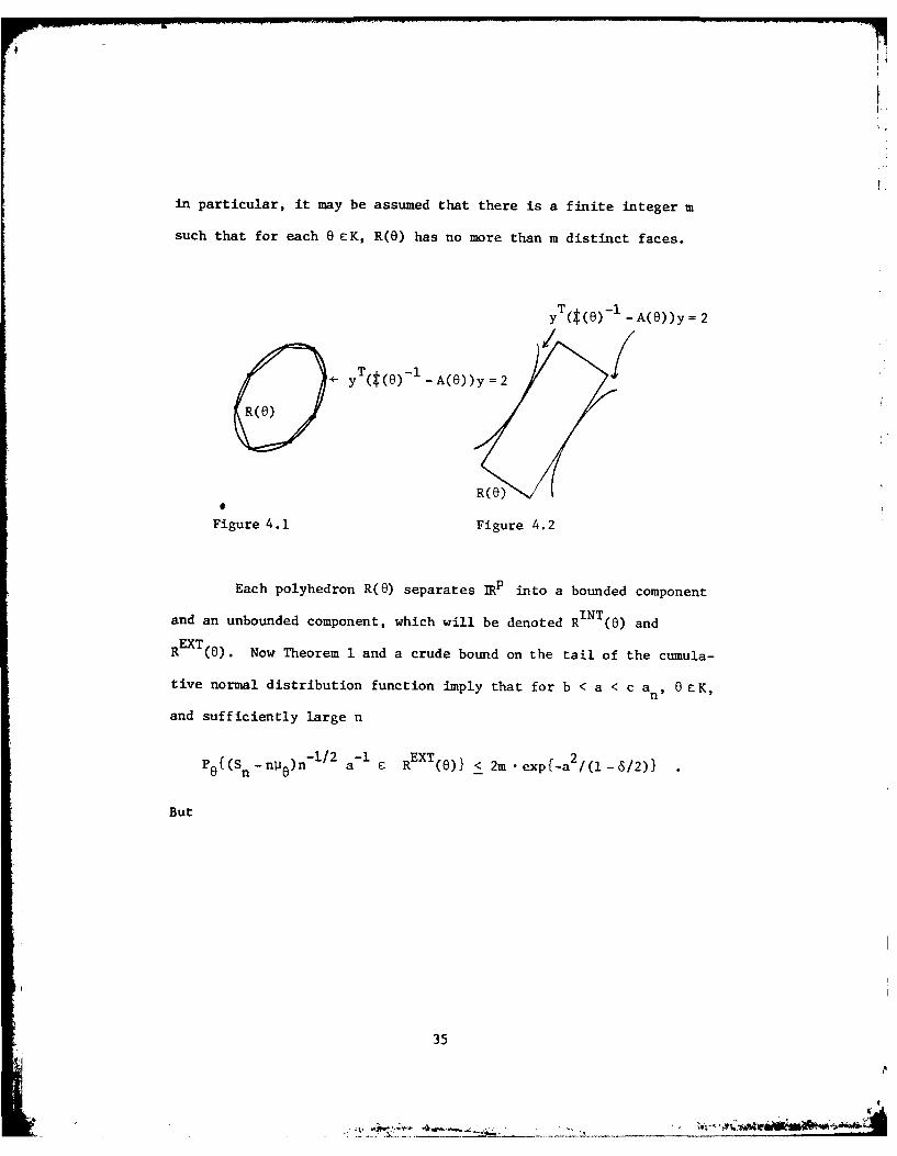
in particular, it may be assumed that there is a finite integer m

such that for each 0 c K, R(O) has no more than m distinct faces.

y T(( 0)-i - A(e))y= 2

R(R)

0

®R(e)(Figure 4.1 Figure 4.2

Each polyhedron R(0) separates IRp into a bounded component

and an unbounded component, which will be denoted R INT(0) and

R EXT(0). Now Theorem 1 and a crude bound on the tail of the cumula-

tive normal distribution function imply that for b < a < c an, 0 EK,

and sufficiently large n

P0 {(Sn )n-/2 a- I REXT() < 2m .exp{-a 2/(l-6/2))

But

35

-1Of/2( -1/2

(4. 10) EO 1 B(n,e) 11g0(o()-/(S n -nil)n - 1 2 >b}

go /2 -n)n1/2)

" E P {(Sn-np0)n-i/ (log b)(i-6/4)- REXT();

isn -nP In- 1/2 <a n

max{g 0 (t(0)- / 2 y)

y C (log1/2 b) (1 - 6/ 4 ) -k/2 REXT(a);

y (log1 /2 b)(1- 6/4)- (k+l )/2 REXT(8)}

2m E expi(log b)[(1 -6/4) - ( k + l ) (1i-6/4) -k(i -6/2)-i]

k=O

for sufficiently large n, and all 0 cK. The series on RHS (4.10) can

be made arbitrarily small by choosing b large; this proves (4.9),

and thus (4.7). //

36

5. Expansion of likelihood Functions

Let N be a smooth, compact, r-dimensional submanifold of r,

and let f() be a smooth, strictly positive probability density on N

(with respect to the "volume element" measure a(-)). Define

(5.1) Q(A) f fN P(y)(A)f(y)a(dy)

thus Q is a probability measure on the a-algebra (X1,X,... ).12*

Furthermore, the measures P6 and Q, when restricted to the a-algebras

3(Xl,... X) (these restricted measures will be denoted P(n) and Q(n)

respectively), are mutually absolutely continuous, and

I ( y ) T S n ( ( )n ) -

(5.2) dP n)/dQ (n) = N e 0)Snn (9(y)) f(y)a(dyJ

The objective of this section is the derivation of a more tractable

expression for dP(n)/dQI(n) when Sn/n is near N, as n o

It will be convenient to have some notation available for

various matrices which will occur. Recall that the tangent space

TN(y) to N at y is the vector subspace of IRp defined by

(5.3) TN(y) = (v EIRp : 1 smooth g : [-1,1] - N

with g(O) = y and g'(0).= v}

thus TN(y) is an r-dimensional vector space, for every y EN. Let

PTN(y) denote the orthogonal projection operator from IRP to TN(y),

and let

(5.4) H1(Y) O W(0(y)) 1 P HP(y)-I

TN(Y) -TN (y) V(y))

37

(5.5) H2(y) - P TN(y) 466(y)) P'T(y) h TN (y)

Note that H2(y) considered as an operator on TN(y) is invertible,

since $(8(y)) is invertible; furthermore, since TN(y) is vector-

space isomorphic to IRr, H2(y) may be interpreted as an operator on

e r , and det H2 (y) is then unambiguously defined.

PROPOSITION 1. Suppose y 1 N, and

(5.6) S nn y- Yl + hn-1 /2

1/1

where Ihi < n- /. Then as n o

(5.7) dP(n)/dQ(n) ~e -n(Sn/n) f(yl) -1 (n/27)r/2

• exp{hT(t(-(yl)) -I - Hl(Yl))h/2}

• det(H 2 (yl)) 1 /2

This relation holds uniformly for y 1 cN and I(Sn/n) -ylj <6n1/7l/2,

for every 6 > 0.

The proof is a relatively straightforward exercise in the use

of Laplace's method. The basic idea is that for large n the only

part of N which contributes to the integral in (5.2) is a small patch

around y1 (essentially of radius n1/71/2 log n), and that the inte-

gral over this patch is approximately equal to the integral over the

tangent space at y,. Because N is compact, all of the errors are

uniformly small.

38

Since the relation (5.7) is crucial to all that follows, the

argument will be given in detail. Taylor's Theorem yields

(5.8) QyTx-iie))-(x (y )T (Qy) 1 (x -Y1.)

(1 - 1.

~1T t^,)-l (

+0(11-y3) +0(fx-_y1 1

3)

by way of the identities

(5.9) =I ve w~l

6 =l V> 4' Vy 1)

$((y)) = ' 2 y

y

Because N is compact, the remainder terms in (5.5) are uniformly

small, i.e., there exist C,6 > 0 such that whenever yl1yE N,

ly-yl1 <6*, and Ixyl<6

(5.10) 0(jxy 13) < Cjx _Y113

0(ly-yII3) <CyyJ 1

3

39

Relation (5.8) may now be used to integrate over the set of

y EN which are within n 1/7 -1/2 log n of y1 . If xEr, and

Ix-yll < 6n1/7- /2 then

T(5.11) fN exp{n[e(y) x ^- P((y)) -4(X)

1/7-1/2l{Iy-yl[ <n log n) f(y)a(dy)

exp{-n(x-Y 1 ) T $((yl))- I (x-yl)/2}

* f(y1 )

f IN expfn(y-y 1 )T *(6(yl)) - (x-Y,)}

•expf-n(y -yl) r $(e(yl)) - (y -y1)/2)

1/7-1/2l(y-yll <n log n) O(dy)

~ expf-n(x-yl)T $(6(yl))-i (x-yl)/2}

. f(y1 )

S[TN(Yl) expfn yT ((yl))- (x-yl))

expf-nyT T(O(yl)) - y/2} m(dy)

where m(dy) denotes the Lebesgue measure on TN(y I). Moreover, the

last relation is valid uniformly for yIcN and Ix-YI n /7- /2

since the curvature form of N at y1 is uniformly bounded

40

(in operator norm) for y, EN (because N is compact). The last

integral may be evaluated exactly by completing the square, leaving

T(5.12) fN exp{n[8(y) x-*(6(y)) -V(x)]}

l{[Jy - y11 < 1/ 7- 1/2 log n} f(y)a(dy)

T Ax _-l

~ exp{-n(x-Yl) $(O(yl)) (x-y)/2}

f(yl) •(2n/n)r/2 (det H2 (Yl)) - 1/2

* expfn(x-y) T H 1(y I ) (x - yl)/2}

Note that since Ix-Y 1 I <6n- /2 +1/7 the last quantity is

never smaller than expf-C' n 21 7}. Thus to complete the proof of

(5.7) it is sufficient to show that the integral over

1 n/7-i/2(y eN :y-yl >n log n} is of smaller order of magnitude.

Now the function

A Tu(y) = 0(y) x-ip((y))- 4(x)

is a nonpositive function of ye r whose only zero is at y -x. The

Taylor series expansion (5.8) for u(y) shows that there exist con-

stants C > 0 and n0 such that for n > n.,

jy1-y > ni1/7-1/2 log n

Ix-Yj < n 1/7-1/2

and Yl eN

41

.1 M Sf&.A-I

imply

YT x * 1+2/7 2(5.13) 6(y) x-i(O(y)) -(x) < C n log n

Consequently,

(5.14) fNexp fn [<^6 (y) I x> - 0 (y)) - W Dx

1{ly-ylj >n1/ 7- 1/ 2 log n) f(y)a(dy)

< exp{-C n2/7 log n}

This completes the proof of (5.7). ///

Let

M0 = {x ERP: O(x) <E and uT x o Vu ETQo(O)}

Suppose that N is a smooth compact r-dimensional sub-manifold of

M0 n r, with boundary, e.g.,

N= - xr 0 A rlI : El < l(x ) - 0 xW < E2< EO

It is possible to mimic the preceding analysis to obtain asymptotic

expressions for likelihood functions, but only when S n/n is not too

near the boundary aN :near DN, N is not well approximated by its

tangent space, but instead by a half-space of its tangent space.

As before, let f(') be a smooth, strictly positive probabil-

ity density on N with respect to the volume element measure a('), and

let

Q(A) fN j8(y) (A)f(y)oa(dy)

42

• .. >., tA

PROPOSITION 2. Suppose yl EN and

-1/2 1/7-1/2(5.15) Sn/n = Y + hn-i and dist(Sn/n, aN) >n log n

1/7with Ihi < 6n . Then as n - I.

(5.16) dP(n)/dQ(n) en(Sn/n) f(yl)-i (n/2) r/2

exp~h -Hl(yl))h/2}

* det(H 2 (Y))1 2

This may be rewritten as

-A -1 r/2(5.17) dP0n)/dQn - e n f(yl) (n/2T)

* exp{hT($C(yl)) - I -H1(Yl))h/2)

* exp-h T H3 (yl)h/2}

(det H2 (yl))1/2

where

(5.18) H3(Y) V 2 i(y) - V2 (Y) + V2 0(y)

Relations (5.16) and (5.17) are valid uniformly on the event

{dist(Sn/n, N) < 6n/7/2 , dist(Sn/n, N) > nI/7 /2 log n}.

Recall that An - n( 1 (S n/n) - 0 (S n/n)) is the log-generalized

likelihood ratio statistic for testing H0 v. H1. It is worth noting

43'p g

a consequence of (5.17): for each compact K C N\N and each 6 > 0,

there is a C > 0 such that

dist(S n/n, K) < Sn- log n

implies

--A n

(5.19) dP n)/dQn ) < e n exp{C log2 n

The proof of (5.16) is essentially the same as the proof of

(5.7), and (5.17) follows simply from (5.16): note that

W S n/n) -n nIl(Sn/n)

= (l/2n)(Sn -ny 1 )T[Vy (Yl) - 2y Y 1(yl)](Sn-nyI )

+ O(n-2iSn-n 1 13)

and

n%0(Sn/n) - (l/2n)(S n nyl )T v2 o(Y)(S n nyl) +O(n-2 Sn -nyl 13)

since O(y1 ) - yl(Y), 7y 0(yl) = Vy l(yl) = 6 (yl), o(yl) = 0, and

V y o(Y = 0 for Y, eMo n rI. That the 0(') terms are uniformly

small follows from the compactness of N. //

44IJ~!

6. The Collapsing Argument

The limiting constants in the conclusion of Theorem 2 occur

as integrals over certain submanifolds of the mean parameter space:

this corresponds to the fact that the bulk of P 0An >n E} andI0

Po[T <a E 1} is accounted for by sample paths for which Sn n and ST/T

are near the critical manifolds. The purpose of this section is to

prove that the probabilities in question actually do shrink to inte-

grals on the critical manifolds (hence the term "collapsing

argument": it is not meant to suggest any structural deficiency in

the proof itself).

Let

T - finf n >a I1 : A >a)a -- - n

IMo M {xEIn 0 (O) : (x) < E o

ME = [x e M0 n 1 r:4 W (x) E)

NE - {x EM0 :(x) = El

PROPOSITION 1. Assume that 0 < E, E2 < % and 0 < El < E < E2 . Then

for every 6, k > 0

(6.1) P OAl>nE; dist(Sn/n,N) > 6n- I log n) o(n - e ) as n ,

and

45

'A.I

....-. kA

-_ a-1/2-k a

(6.2) P0 {Ta<aClI; dist(S T/T, Na/T) >Sa logal o(a -k e - a )

as a -* OD

The proof will proceed by a series of crude estimates based

on a likelihood ratio identity. The first step is to show that only

those sample paths for which the sample means S /n fall in a certainn

compact subset of IRp are of any consequence.

LEMMA 1. There is a compact set K c r such that x cK implies

O(x) < %; also

(6.3) {x r : (x) <max(E, E2} C K0

and

-mE3(6.4) P { an>m : S n/n K) = o(e )

as m o, for some 3 > max(E, E 2 ).

PROOF. Choose E3,E4 so that

max(EE 2 ) < < E < E

Then the sets

K3 fx cr _W<x )

K4 = {xE :4(x) <E 4 )

are compact (this is the reason for condition I on E), and K3 is

contained in the interior of K4 . Thus there is a compact K contained

46

II

in the interior of K4 and containing K3 in its interior, whose

boundary AK is a polyhedron (i.e., K is the intersection of finitely

many half-spaces). The existence of K may be deduced from the

finite-dimensional Krein-Milman Theorem, the compactness of AK4, and

the convexity of 4.

Figure 6.1

Now Chernoff's large deviation theorem for random variables

(cf. [41) gives exponential bounds for P 0{S n/n t H} where H is any

half-space; since K is the intersection of finitely many half-spaces,

and since 00

PO0f n>m :S /n tK} < E P(S /nOK]nm

(6.4) follows easily. ///

Let f() be a smooth probability density on r (with respect

to Lebesgue measure on IRP) which is strictly positive on K. Define

47

tLi4

(6.5) Q(A) = 'r P (y) (A)f(y)dy

th n f) adp(n)then Qn) and P0n (the restrictions of P0 and Q to the a-algebra

5(xI ... oX)) are mutually absolutely continuous, and

6F (y)TS nn(6(Y)) y I

(6.6) dpn)/dQ(n) = e f(y)d

LEMMA 2. There is a constant C > 0 such that

(6.7) [dP /dQ)] lfSn/ncK} < C- n 2 p e- S0 n

PROOF. To obtain an upper bound for (6.6), one may replace the

domain of integration r by a p-dimensional cube of side i/n2 centered

at S /n. Since K is compact and f(-) has a strictly positive minimumn

on K, (6.7) follows routinely. ///

To prove Proposition 1 it now suffices to show that there is

a constant 3 > 0 such that if x eK, E1 < b < E 2 , and

(6.8) l(X) - 00(x) > b

and

(6.9) dist(x, Nb) > 6n- 1/ 2 log n

then

(6.10) W(x) > Rn-1 log 2 n + b

For then Lemma 2 would imply

48

:6.11) Po{An>4E; dist(S n/n, NE) >6n-1/2 log n; Sn/n cK}

< C n2 p f e -nE e- log2 n dQ

and

(6.12) P 0 (Ta<a~ 1 ; dist(ST/T, Na/T) >61/2logn; ST/TcK}

-8 log2 (aE I )

< C(aq 12 p f{.}e - a e dQ

LEMMA 3. For every 6 > 0 there exist y > 0 and > 0 such that if

xcK and E < y

(6.13) dist(x, F) > 6E

implies

(6.14) (x) - >(X) >

PROOF. First recall that -i is a no-.-negative function of x CF

which is zero only for x e F: consequently, it suffices to cons-.der

only those x eK for which

(6.15) dist(x, F1) < r)

where n is a small positive number of our choosing. Now n may be

chosen so small that for x c K satisfying (6.15) x c U1 and the MLE map

01 is submersive in a neighborhood of x (cf. Lemma 1, Section 3), and

also small enough that for x CK satisfying (6.15) the two-term Taylor

49

j1

~e

series for ( -4i) around P^(X) is accurate enough that

(6.16) (x) -l(X) 1016 l(X) - 0 l(lX ) )

T

+ (x- 11( x))Tv( -¢l)( 1x)

1 1+ (1/) (x 16 TV2 M x-V

Since ( 1 it follows from Lemma 1 of Section 3 that1() 1

W1x 1 1 (x)

and

Thus to prove (6.14) it suffices to show that for x EK satisfying

(6.15) there exists a 6 > 0 such that

(x P($ ) i (T )(x- ^ > 6(dist(x, FI 2

Notice first that x-P^( £T V (l (x)) , and recall that

V 21 (il(X) ( M I(a(x)) = 0 (this is (3.14) of Lemma 1, Section

3). Thus by the compactness of K and the fact that

7' 4(y) = Z(O(y))-1 is everywhere P.D., there exists a 6 > 0 such

that whenever x CK satisfies (6.15),

0 l(xl 1(x) 01(X)

50

Since pl^X) C ri it is clear that

(6.18) Ix - ( )I > dist(x, rI)

This proves (6.14). /

LEMMA 4. For each 6 > 0 there exist y > 0, 6 > 0, and $ > 0 such

that if xEK, E<y, and

(6.19) dist(x, MO) > 6E

but

(6.20) dist(x, F1) < 6

then

(6.21) 0(x) > BE

PROOF. O0(x) is a convex non-negative function of xc K which is zero

iff xC M0. Thus it suffices to consider only those x eK for which

dist(x, M0) < n: here n > 0 is a constant of our choosing.

Recall that M0 and F1 intersect transversally whenever they

intersect (this by condition III in the definition of E0). By

Lemma 2 of Section 3 there exist 6 > 0, n > 0 small enough that if

x cK satisfies (6.20) and

(6.22) dist(x, M0) < ,

then

(6.23) dist(x, M0 fn rl) < ri

51

r*

Here q > 0 has been chosen small enough that if x cK satisfies

(6.23), then x cU 0 and the MLE map 60 is a smooth submersion in a

neighborhood of x, and in addition the two-term Taylor series for 0

around P W (x) is accurate enough that-o (0)

(6.24) *0(Px) +(x-Px) T Vo(Px) +(1/4)(x -Px)T V2 0 (Px)(x- Px)

= (1/ 4 )(x -Px)T 2 o(Px) (x - Px) < 0 (X)

(P =P _ denotes the orthogonal projection onto TQo(O )M o(0) 2

By Lemma 1 of Section 3 V2 o(y) is strictly P.D. on TQ0 (0)

for any y such that 80 (y) = 0; since x-Px t T%0(0) the lemma follows

from (6.18) and an obvious compactness argument. //I

LEMMA 5. For every 6 > 0 there exist 6 > 0, 8 > 0, and y > 0 such

that if E < y, and x E r satisfies

(6.25) dist(x, M0 fl r1) < 6 E

(6.26) dist(x, Nb) > 6 E

and

(6.27) O(x) > b

then

(6.28) O(x) > b + OE

Here Nb = (ycM0 n rl :0(y) b), and (6.28) holds for all b such that

E < b < 2 (for the same B).

52

PROOF. It follows from Lemma 2 of Section 3 together with condition

III in the definition of E that there exist 6 , , and y such that

if xcr satisfies (6.19)-(6.20), then

(6.29) dist(x, {ycr : (y)-b)) > a E

If x also satisfies (6.27), then

(6.30) dist(x, tycr : 4(y) <b) > E

Relation (6.28) follows directly, since V is nonzero on the level

surface {y er :4(y).=b. That it holds uniformly for E b < _

follows from an easy compactness argument. //

It now follows from Lemmas 3-5 that if x K satisfies

(6.8)-(6.9), then it satisfies (6.10) (since 1>JI 0 >0). This

proves Proposition 1. /1

53

7. Proof of Theorem 2

The proof of Theorem 2 will be based on the likelihood ratio

identity

(7.1) P (A) - fM[ E- 1A L T]OM(dy) /cf(M)

where

(7.2) M= WE 5 ' E 6 ; 0) = {y E r1 f in20 (0) :E5 (:S1 (y) %(y) <E 6

(7.3) 0< E5< E 1 < 2 <E 6 < E

(7.4) LT =d(P0 UT)/d(Q T

and

(7.5) Q(B) = P^ (B)a (dy) /0(M)0 (y)

Recall that M is a compact manifold-with-boundary, so its total sur-

face area a(M) is finite. The relation (6.1) holds for all events

A cUT OT is the "stopped" sigma algebra of events A for which

A n {T <n) c.3(X1 9**,X n )I for every n) and (7.5) holds for all

According to Proposition 1 of Section 6,

(7.6) P{T <aE1 ; dist(S M(Ej, 0) 1 ~ /2 lga a

as a 4 ,for all k,S > 0. Consequently, it suffices to show that

(7.7) P (A) -RUS (3.22)0

for the event

54

(7.8) A- ;T a-1/2 log a > dist(S T/T, M(E,E 2 ;O))}

The plan of the proof, then, will be to evaluate (7.1) for A defined

in (7.8) by exploiting the asymptotic formula for 1 A L T provided by

Proposition 2 of Section 5.

NOTE: Throughout the rest of this section, A will be the event

defined by (7.8).

'I The manifold M divides neatly into three zones, in each of

which the integrand behaves differently. These are

-1/2 +r) () ()<E-a-1/2Tj(7.9) M, {y -M : E,+a- ~ 1 y 0 (y 2 4

M2 - f{y M : ' l (y - ' O'y) <. 'i + a-/ n or

-12 /j

nfl y e M : dist (y,M(E 1 , E2 ;O0)) < a1/ 2Tj

-1/2 +rjM3 {y E M : dist(y,M(E1 , E2 ;0)) >a

where 0 < n~ < 1/32 is some fixed constant. It is clear that

1 t E, 2 ;) and that 3M +a(E 1 ,E2 ;O) (tu4( 2 0 as a .o)

It will develop that I -RHS (3.22) and that f and fm are ofMl M2 3

smaller order of magnitude.

For y c M, define

55

(7.10) nI = nI(a,y) - ( (y) - (y))) - a 1/ 2 +T13

n2 . n2 (a,y) - (a/( l(y) _ o(y)) ) -a1/2 +n/2

n 3 = n3 (ay) - [ (a/( 1 (y)_ 0 (y))) +al/2 +r/2

(7.11) ln(y) (n- ny)T(t(Q(y))-l-1(y) - H3(Y))(Sn-ny)/2n ,

where H1 (y) and H3 (y) are as in (3.26) and (3.28).

LEMMfA1. Asaaw

(7.12) max P ISn -nyl >C a1 2 + some nc[a aE1ycM

- o ( e ) ,

(7.13) max P ()T [n2 (a,y), n (a,y)]) = o(e- )yEM 1 ecy) a 23'

(7.14) max P^' (y) - (Y) > C/log a, some ne [n2ny(y)yCM O~) n n1 2

1/16O-ao(e- ) ,i:

andI.

(7.15) max P- ( (S /n) -(S /n )I > C a-1 /2 log2a) -

yEM (y) n n o a

for all C > 0, 0 < 8 < 1/6.

56

. . . . .. . -& :. ?_,Z', " ,.,.::, =,= , _a, . .. . .. . .. . :,., ,n.- . - i . . ,-' ' ''

' " "'',,- . .~- '

This is a routine consequence of Corollary 1, Section 4; the

proof is left to the reader.

Next define events

(7.16) A~ y {(S nn 1-y <a1/2 +n

A* f I(S /n).(S /T) I <a1/2 log a}y n 1 i T

A* A* {T c(n Ca,y),n (a,y)Iy y a 23

By Proposition 2, Section 5

-A qqo/

(7.17) LT 'A1'A '*- e T exp{C y} T2ry

(det H 2(y)) 1/2 G(M)l A A 1A*y y

and

-A(7.18) L 1 1A 'A e* T expfC n (y)la(M)l AIA IA**

y y 1y y

. (a/2ir( 1 (y) - O(y))) 1

. (detH2()1/

furthermore, these relations are valid uniformly for yc M and uni-

formly on the events A y1)A A*, and A ynA A**, respectively.

57

LEMMA2. As a ,

-(A T-a)(7.19) Py(Y) 6(y)[A1A**e T In 1 (a,y)]-VCy)I >E} + 0

yt

for every E > 0 and every y EM(E,,E2 ;0) such that the random variable

(01 (y) - o(y)) + (Xl1 y)T 7(o )(y )

has a nonlattice distribution when X Pb(y) (cf. Lemma 4,

Section 3).

The O-algebra .3 is the one generated by X1 ,... ,X Itni ni

should be noticed that the convergence indicated by (7.19) need not

be uniform in y. Fortunately, the rv's are bounded.

Lemma 2 is very much related to the nonlinear renewal theorem

of Lai and Siegmund [9]. Although the statement of their theorem

does not imply Lemma 2, their proof does: in fact, they obtain an

unconditional limit theorem by first proving a conditional statement,

which in our case becomes

(7.20) Eg(y)[eT 3 nl - v(y) - 0 A.S. (Pb(y))

Since 1A lA** - 1 (cf. Lemma 1) A.S. (P(y)), (19) follows from this.

yThe key to evaluating EA(y) 1A 1A lA,* LT is now provided by

y yCorollary 2 of Section 4. This allows that uniformly for y EM,

(7.21) E§(y) 1Ay exp{ n(a y) 1 -(det (8(y)) (H (y) +H3 (Y)))- 1 /2

58

-tt*Lmn A re fgaL"

Im

as a - 0. Consequently by (7.18), (7.19) and the Dominated

Convergence Theorem

-~(q-qO)/2 a r* T

(7.22) aMI e E§(y)[1Ay OM(dy)/cfM(M)

+ c(EE 2 ;0)

Recall from Proposition 2 of Section 5 (5.19) that

-AT

(7.23) 1A LT < e exp{C log 2n}

for some constant C. By Lemma 1

max P^(y) (A(Ay 1 A** o(e-a / 4

mxfAy )) = o)e;YcM I P(y)(A(A

thus

(7.24) a- aql 2 e a E 5(y)[iA\(A fA**) LT 0 y(dY)/GM(M)

y y

0 as a-4 0

For y cM, (7.17) and a compactness argument show that there29

is a constant C > 0 such that

-(ql-q0 )/2 a<C x{na e aL T I AfA (-A* <-- ep (Y)) } A y

Y Y

and (7.21) Implies that there is a constant C** > 0 such that

-(ql-qO ) /2 **

E~'A ea L I _(y) a T Aff, <A*y y

59

This, (7.23), and the fact that

, o~e-a/ 4

max P-() (A\(A n A)) o(ea )

YEM2

imply

-(ql-qO) / 2 -

(7.25) fM2 a e E3(y) LT 1A OM(dy)/oM(M) 0

since cM(M 2) - 0.

Finally, for y EM39

(7.26) A n{ISn/n-yj <a-l/2 +/2 for all n c [a1,aEl]J =

By Lemma 1

max P6(y){IS n/n l -y >a-l1 2+/2 for some n c[a 2 ,aEl 1 ]}YEM 3

o(e-a / 4

this (7.23), and (7.26) imply

F -(q 1 -qO) /2a

(7.27) f a ea E [(y)u1A LT] aM(dy)/((M) + 0

The relations (7.1), (7.22), (7.24), (7.25), and (7.27) prove

Theorem 2. //

60

REFERENCES

[1] Armitage, P. (1967). Some developments in the theory andpractice of sequential medical trials. Proc. 5th BerkeleySymposium 4, 791-804.

[2] Armitage, P. (1975). Sequential Medical Trials, 2nd edition.Oxford: Blackwell.

[3] Bhattacharya, R., and Ranga Rao, R. (1976). NormalApproximation and Asymptotic Expansions. John Wiley andSons, New York.

[4] Chernoff, H. (1952). A measure of asymptotic efficiency fortests of a hypothesis based on the sum of observations,Ann. Math. Stat. 23, 493-507.

[5] Efron, B. (1975). Defining the curvature of a statisticalproblem (with applications to second order efficiency)(with discussion). Ann. Statist. 3, 1189-1242.

[6] Feller, W. (1968). An Introduction to Probability Theory andits Applications, Volume 1, 3rd edition. John Wiley andSons, New York.

[7] Feller, W. (1971). An Introduction to Probability Theory andits Applications, Volume 2, 2nd edition. John Wiley andSons, New York.

[8] Guillemin, V. and Pollack, A. (1974). Differential Topology.Prentice-Hall, Englewood Cliffs, New Jersey.

[9] Lai, T.L. and Siegmund, D. (1977). A nonlinear renewaltheory with applications to sequential analysis I.Ann. Stat. 5, 946-954.

[10] Lai, T.L. and Siegmund, D. (1979). A nonlinear renewaltheory with applications to sequential analysis II. Ann.Stat. 7, 60-76.

[111 Schwartz, G. (1962). Asymptotic shapes of Bayes' sequentialtesting regions. Ann. Math. Stat. 33, 224-236.

[12] Siegmund, D. (1977). Repeated significance tests for a normalmean. Biometrika 64, 177-190.

[13] Siegmund, D. and Gregory, P. (1979). A sequential clinicaltrial for testing PI-p 2 " Stanford University TechnicalReport.

61

[14] Woodroofe, M. (1976). Frequentist properties of Bayesiansequential tests. Biometrika 63, 101-110.

[15] Woodroofe, M. (1978). Large deviations of likelihood ratioswith applications to sequential testing. Ann. Stat. 6,72-84.

[16] Woodroafe, M. (1979). Repeated likelihood ratio tests.

Biometrika 66, 453-463.

62

UNCLASSIFIEDSECURITY CLASSIFICATION OF THIS PAGE (W"en Data Entered)

READ INSTRUCTIONSREPORT DOCUMENTATION PAGE BEFORE COMPLETING FORM

I. REPORT NUMBER 2. GOVT ACCESSION NO. 3. RECIPIENT'S CATALOG NUMBER

No . 1 0 -d ,

4. TITLE (and Subtitle) S. TYPE OF REPORT & PERIOD COVERED

TECHNICAL REAT.,REPEATED LIKELIHOOD RATIO -JESTS FOR I R T

1URVED EXPONENTIAL FAUILIES 6. PERFORMING ORG. REPORT NUMBER

17. -AUTHOR(O'I 8. CONTRACT OR GRANT NUMBER(.)

STVT ALLEY ) 'NO00014-77-C-0306

1. 1 -, .ANIZATION NAME AND ADDRESS t0. PROGRAM ELEMENT. PROJECT. TASK

DEPARTfENT OF STATISTICS AREA 6 WORK UNIT NUMBERS

STANFORD UNIVERSITY NR-042-373

STANFORD, CALIFORNIA ( - -

11. CONTROLLING OFFICE NAME AND ADDRESS 12. REPORT DATE

OFFICE OF NAVAL RESEARCH SEPTEMBER 1, 1980STAT. & PROBABILITY PROGRAM, CODE' 436 13. NUMBER OF PAGES

ARLINGTON, VIRGINIA 22217 6214. MONITORING AGENCY NAME & ADDRESS(It different from Controlling Office) IS. SECURITY CLASS. (of thil report)

A-..-rI UNCLASSIFIED-, IS.. DECLASSIFICATION/DOWNGRADING

SCHEDULE

16. DISTRIBUTION STATEMENT (of this Report)

APPROVED FOR PUBLIC RELEASE AND SALE: DISTRIBUTION UNLIMITED.

17. DISTRIBUTION STATEMENT (of the abttact entered in Block 20, It dilferent from Report)

I8. SUPPLEMENTARY NOTES

19. KEY WORDS (Continue on reveree side I necessary and Identify by block number)

Curved Exponential Family, Repeated Significance Test,Nonlinear Renewal Theory, Transversality.

20. ABSTRACT (C.vth m rovere. 1* Ft nceswr and IdeWfity by block number)

A class of repeated significance tests for curved hypotheses in multi-parameter exponential families is studied, and asymptotic formulae for thesignificance levels of such tests are obtained. Special attention is giventhe important case of comparing Bernoulli success probabilities.

DOR ' IF006I OmEITION4 OF I NOV SS IS, OWSLETZF.,

JAN 73 UNCLASSIFIED

SECURITY CLASSIFICATION OF THIS PAGE (Ilibet Data Entered)

.. .. ")-. • ?"= -. . --_ ". ". v " 'k ', : ) :: ", ".