ad-ao13 397 handbook fop the direct statistical analysis … · 2011-05-13 · statistical analysis...
TRANSCRIPT

AD-AO13 397
HANDBOOK FOP THE DIRECT STATISTICAL ANALYSIS OFMISSILE GUIDANCE SYSTEMS VIA CADET'M (CGVARIANCEANALYSIS DESCRIBING FUNCTION TECHIIQUE)
James H. Taylor
Analytic Sciences Corporation
Prepared for:
CIffice of Naval Research
31 May 1975
DISTRIBUTED BY:
Nationli Technical Infermation ServiceU. S. DEPARTMENT OF COMMERCE

ct4%
LLSo
A.
q Reopmdiamd byNATIONAL TECHNICALINFORMATION SERViCE
US Ihg~mbfetI eA Com,~mmeWadg"ll. VA. 2213i

•'• • ,,• . ,, , , -. ,,:- M ,t,, -- nr•..c.... . L--- ,r-, 'g r n'..uy*'r-wrn- 1'K•wr-n •xr-w- '''. - - -.... .. . . " .. ......
UNCLASSIFIEDSECURITY CLASSIFICATION OP THIS PAGE (When D0el* snreitrd)
REPORTy DIU TA~LIpAY N-PbAGE~ READ INSTRUCTIONSREPOR CM ENTIO~N PAGE BEFORE COMPLETING FORM.I. REPORT NUMBER GOVT ACCESSION N". S. RICIPIINT'S CATALOG NURISR
TR-385-24. TITLE (d Subtitle) .... S. TYPE OF REPORT & PERIOD COVERED
4.HANDBOOK FOR THE DIRECT STATISTICAL Technical Report_ 1ANALYSIS OF MISSILE GUIDANCE SYSTEMS March 1974 - 31 bec.1974VIA CADETTM *. PERFORMING ORO. REPORT NUMBERTR-385-P,
S•~. AUTHNO1(o) ... .... S. CONTRACT Oft GRIANT NUMSI•WUO)
James H. Taylor N00014-73-C-0213
S. PERfORMiNG ORGANIZATION NAME AND ADDRESS Z. R AM ELEMENT, PROJECT, TASK'ARRA a WORK UNIT NUM6901S
"The Analytic Sciences Corporation6 Jacob Way ONR Task No. NR-215-214Reading, Massachusetts 01867
II. CONTROLLING OFFICE NAME AND ADDRESS I1. REPORT OAT3
THE OFFICE OF NAVAL RESEARCH 31 May 1975Vehicle Technology Program Code 211 13. "UMBEROFPAG09%A hrlina-on, Virginia 22217 ,'O
S14. MONITORING AGENCY NAME &ADDRIESS(Il @•deilearo trin Controlling Office) IS, SECURITY CL.ASS. (fo thte report)
UNCLASSIFIED
SIS*. OCCL,•Si.FC ATi0NIOOWNGPIAISIP ;•, ~SCH~ROULE
6" bSTRIDUTION STATEMENT (of ?Ate RepotI)
Distribution of this Report is Unlimit•.d.
17. DISTRIBUTION STATEMENT (of the abetract entered In Blott 20, It dllferenlt rom Report)
IS. SUPPLEMENTARY NOTES
Is. KEY WORDS (Continue, oan r.vere* *ide f necesry and Identify by block number)
Missile Guidance SystemsCovariance AnalysisNonlinear Systems (Continuous/Discrete)Describing Functions (Random Input)
20. ABSTRACT (Continu. on rver.sir ddr It n.e..sy nd Identify by block number)
This Handbook presents detailed instructions for theapplication of the Covariance Analysis DEscribing FunctionTechnique (CADETTM)-to the evaluation of tactical missileguidance systems (both analog and digital). Its contentsinclude: CADET theory, simple illustrative examples (withflowcharts), model development for the missile-target
DD EOA" 1473 EDITION OF I1OV65 1S OUSOLEE UNCLASSIFIEDReproduced by XCURITY CLASSIFICATION OF THIS PAGE (Wh..en Dile tntefed)NATION4AL TECHNICALINFORMATION SERVICE
U 5 ODeparment ol CommerteSpetnglii.d, VA. 22151

UNCLASSIFIEDSECURITY C6ANWIt CATAOw OPr TWIlG PAlEflSMOM Does 54.
kO. ABSTRACT (continued)
intercept problem, statistical linearization theory, dis-cussions of the capabilities, limitations, and applicationphilosophy of CADET, and an extensive catalog of pertinentrandom input describing functions. A detailed discussionof monte carlo analysis is appended, both to permit a compari-son with CADET and to provide a background for the monte carloprocedures used to verify CADET.
Ii
II
UNCLASSIFIED
SECURITY CLASSIFICATION OP THIS PAOR(MWm Data Fated0
i'I
'rHE ANALYTIC SCIENCES CORPORATION
TH-385-2
HANDBOOK FOR THEil DIRECT STATISTICAL ANALYSIS OF
MISSILE GUIDANCE YSTEMSVIA CADETTV
1 31 May 1975
I Prepared Under:
Contract No. N00014-73-C-0213(ONR Task No. NR-215-214)
for
THE OFFICE OF NAVAL RESEARCH-Vehicle Technology Program, Code 211
Arlington, Virginia 22217 "hJLA -
Reproduction in whole or in part Prepared by:is permitted for any purpose of James H. Taylorthe United States Government.
Approved for public release;distribution unlimited. rhlaries F. Price
Arthur A. Sutherland, Jr.
THE ANALYTIC SCIENCES CORPORATIONI6 Jacob Way
Reading, Massachusetts 01867
"" iL

TH, ANALYTIC SCIENCES CORPORATION
FOREWORD
This handbook is the culmination of research
performed on the Covariance Analysis DEscrib-A' ing Function Technique (CADETTM) during a two-year period under Contract N00014-73-C-0213,for the Office of Naval Research. The Sci-entific Officer who monitored and encouragedthis inv,,stigation was Mr. David Siegel.
e I:
' I
V 3I,
Iiii
I
THE ANALYTIC SCIENCES CORPORATION
I-!
I ABSTRACT
The Covariance Analysis DEseribing FunctionTechnique (CADE•TM) -- a-technique conceived'and developed aLt TASC for the efficient directstatistical analysis of nonlinear systems withrandom inputs -- has been proven to provJ,'eaccurate tactical missile performance projec-tions with a small fraction of the computertime expenditure required for a comparably
reliable monte carlo analysis. This handbookis a self-contained, detailed exposition of
the application of CADET to the missile-targetintercept problem. The broad scope of thisdocument is intended to permit the direct analy-sis of a wide variety of nonlinear and randomeffects in missile guidance systems, and tofacilitate and encourage the study of other non-linear systems via CADET.
IvI!
SV

I .-
THE ANALYTIC SCIENCES CORPORATION
I
TABLE OF CONTENTS
I PageNo.
I FOREWORD iii
I ABSTRACT v
LIST OF FIGURES ixLIST OF' TABLES xli
PROLOGUE AND READER'S GUIDE X1li
1. TiE COVARIANCE ANALYSIS DESCRIBING FUNCTION TECHNIQUE(CADET)S1.1 Cova-iance Analysis for Linear Systems 1-11.2 Covariance Analysis for Nonlinear Systems 1-41.3 Continuous/Discrete-Time Systems 1-12
S2. CADET APPLICATION: SIMPLE ',LUSTRATIONS21I Missile-Target Equations of Motion 2-1z.2 The Continuous-Time Case: Proportional Guidance 2-32.3 Guidance Systems With Digital Data Processing 2-10
3. MODEL DEVELOPMENT FOR THE MISSILE-TARGET INTERCEPTPROBLEM3.1 Elements of the Model 3-13.2 The Missile-Target Kinematics Model 3-13.3 The Target Model 3-53.4 The Autopilot-Airframe Model 3-7
3.4.1 Linear Airframe Dynamics 3-93.4.2 Nonlinear Airframe Dynamics 3-12
3.5 The Guidance Subsystem Model 3-183.5.1 Proportionai Guidance 3-203.5." Modern Digital Guidance Systems 3-23
3.6 The Seeker Subsystem Model 3-34n 3.6.1 Boresight Error Distortion 3-34
3.6.2 Disturbance and Control Torques 3-403.6.3 Transfe- Function Representation of the
Equivalent Linear Seeker 3-443.7 System Mod 4l Summary 3-50
U i1
THE ANALYTIC SCIENCES CORPORATION
TABLE OF CONTENTS (Continued)
Page"No. I
4. QUASI-LINEARIZATION: PRINCIPLES AND PROCEDURES4.1 CADET and Statistical Linearization 4-1 V4.2 Princ,ples of Quasi-Linearization 4-3 I.4.3 Random Input Describing Function Calculations 4-12
4.3.1 Single-Input Nonlinearities 4-12 t4,3.2 Multiple-Input Nonlinearities 4-18
4.4 Effects of Different Probability Density Functions 4-264.5 Describing Functions Not Existing in Closed Form
Under the Gaussian Assumption 4-34
5. OVERVIEW AND ASSESSMENT OF CADET5.1 Direct CADET-Monte Carlo Comparisons 5-1 T}
5.1.1 Overview and CADET Mechanization 5-1 I5.1.2 Accuracy and Efficiency 5-2
5.2 Other Factors and Philosophy of Application 5-65.3 CADET Development to Date: Summary and Conclusions 5-9
5.3.1 Summary 5-95.3.2 Conclusions 5-11
APPENDIX A A CATALOG OF RANDOM INPUT DESCRIBING FUNCTIONS A-1
APPENDIX B EXTENSIONS OF CADET B-1
APPENDIX C THE MONTE CARLO METHOD: APPLICATION AND RELIABILITY C-1
REFERENCES R-1i
viii

tHE ANALYTIC BCIENCEB PORPORATION
,I5 LIST OF FIGURES
Figure PageNo. No.
1.1-i Represontation of the Continuous-Time Linear Dynamic5 System Equations 1-2
1.2-1 Nonlinear System Block Diagram 1-4
3 1.2-2 Nonlinear Covariance Analysis -- CADET 1-10
1.2-3 Taylor Series Linearization of y x 3 About mx = 1 1-11
1.2-4 Quasi-Linearization of y - x 3 for Unity Input Mean 1-12
I 1.3-1 An Example of a Mixed Continuous/Discrete System 1-13
2.1-1 Missile-Target Planar Intercept Geometry 2-2I 2.2-1 Simplified Missile-Target Intercept Model. WithContinuous-Time Guidance 2-41
2.2-2 Flow Chart for the Direct Statistical Analysis oi aContinuous-Tir.i System via CADET 2-8
2. 2-:1 Performance Projections for Various Levwls of AirframeAccoleration Saturation 2-9
2. 3-i Simplified Missile-Target Intercept Model With DigitalI Guidance 2-11
2.3-2 Flow Chart for the Direct Statistical Anaiysis of aMixed Continuous/Discrete-Time System via CADET 2-15
5 3.1-1 Basic System Black Diagram 3-2
3.2-1 Target-Missile Planar Intercept Geometry 3-33 3.2-2 Block Diagram Formulation of Missile-Y.-get Kinematics 3-4
3.3-1 Band-Liajited Gaussian Noise Model for Target LateralAcceleration 3-6
:1.4-1 Geometric Definition of Intercept-Plane System Variables 3-8
3.4-2 Compensated Missile Airframe Dynamics 3-11I 3.4-4 typical Nonlinear Representation of the Autopilot/
Airframe Module 3-19
S3.5-1 Deviation from the Collision Course Triangle 3-21
3.5-2 Proportional Guidance Law Model 3-233.5-3 Missile-Target Intercept Model for the Derivation of
the Digital Guidance Modlule 3-25
ix

S•~ m •i , .. . • :•... . :• ••J. • .- . W fl . - -- ... f ~.. ... - -
THE ANALYTIC SCIENCES CORPORIATION
LIST OF FIGURES (Continued)
Figure PageNo-. No.
3.5-4 Digital Guidance Module Based on Optimal Estimation anuControi 3 32
3.5-5 Complete Digital tuidance Module Structure 3-34
3.6-1 Seeker System Configuration 3-35
3.6-2 Boresight Aberration Model J-36
3.6-3 Nonlinear Angular Aberratioa Characteristic Investigatedin Ref. 3 3-35
:1.6-4 Seeker Noise Model 3-38
3.6-5 Receiver Boresight Error Distortion Effects 3-39
3.6-6 Final Boresight Error Measurement Model 3-40
3.6-7 External Disturbance Torque Models 3-42
3.6-8 Nominý.l Seeker Track Loop (Neglecting All NonlinearEffects) 3-44
3.!-9 Complete Seeker Model 3-45
3.6-10 Linear Seeker Model 3-47
3.6.-11 Linear Seeker Model in Transfer Function Form 3-48
3.7-1 A Complete Missile-Target Intercept Model 3-51
4.2.1 Example of a Nonlinear System With Desirable Separationof Nonlinearities by Linear Dynamics 4-8
4.4-1 Three Density Functions Comprised of Two Triangles 4-27
4.4-2 Random Input Describing Function Sensitivity for theLimiter 4-30
4.4-3 Random Input Describing Function Sensitivity for thePower Law Nonlinearity 4-31
4.4..4 Random Input Describing Function Sensitivity fc.' theSinusoidal Operator 4-33
4.5-I Comparison of A proximations for the Expected Value ofthe Range 4-39
5.2-1 Illustration of ( 'DET and Monte Carlo Analysis in aParameter Trade-Off Study 5-3
x
THE ANALYTIC SCIENCES3 CORPORATION
LIST OF FIGURES (Continued
Figure Page..No. No.
5.2-2 Ph~losophy of CADET Application 5-9
SA.I-1 Basic Piecew ise-Linear Character istics A-3
A.1-2 Decomp',.'tion of Complicated Piecewise-LinearCharacteristics ibt,+ lasic Components A-6
B12-l A Product Nonlinearity Driven by Random Biases B-3
L.3-1 Dynamic System With a Product-of-States Nonlineaiity B-8
13.3-2 Simulation Results for a System Containing a Product-of-States Noniinearity B-10
B .3-3 Modified CADET Solution for the System Shown inFig. B.3-1 With Only One State Assumed Nongaussian 13-12
C.1-1 Nonlinear System Model C-2
C.1-2 3chematic Characterization of the Monte Carlo Technique C-5
C.2-1 Typical Confidence Interval Multipliers for thf Esti-mated Standard Deviation of a Gaussian Random Variable(A - 3) C-I1
C.2-2 Effect of Kurtosis on Confidence Interval Limits C-12
C.3-1 Time History of rms Missile-Target Lateral Separation C-1l4
C.3-2 Comparison of CADET and 1onte Carlo rms LateralSeparation C-15
[I,
I
IIS~xi

THE ANALYTIC SCIENCES CORPORATION
",IST OF TABLES
Table PageNo. No.
3.4-4 Example of Compensated Linear Missile Airframe Data inthe Terminal Homing Phase 3-13
3.6-1 Typical Nominal Seeker Specifications 3-49
3.6-2 Typical Nominal Compensated Seeker Specifications 3-49
5.1-1 Comparison of CADET and Monte Carlo Efficiency Based
on 256-Trial Monte Carlo Analysis 5-5
C.2-1 Some Common Probability Density Functions C-7C.2-2 Cumulative Probability Within no Standard Deviations
of the Mean for a Gaussian Random Variable C-9
C.3-1 Estimated Standard Deviation and Kurtosis for LateralSeparation, t = 6 sec C-17
C.4-1 90 Percent Confidence Interval Limits, Gaussian RandomVariables, q Trials (no = 1.645) C-20
C.4-2 95 Percent Confidence Interval Limits, Gaussian RandomVariables, q Trials (no = 1.960) C-21
C.4-3 99 Percent Confidence Interval Limits, Gaussian RandomVariables, q Trials (no = 2.576) C-22
Ii
xii

THE ANALYTIC SCIENCES CORPORATION
PROLOGUE AND I'.EADER'S GUIDE
The development of a complex weapon system with stringent
performance specifications, such as a tactical missile, generally
requires several phases, including preliminary design and feasi-
bility studies, decisions concerning implemen-ation of various sys-
tem functions, and compensation or design modi.ication to obtain
the best possible system performance under realistic constraints.
In the later stages of development, the mathematical system model
used as a basis for generating system performance projections in-
evitably contains nonlinear effects and random inputs. Nonline-
arity is generally associated with nonlinear relations inherent
to the laws of physics, unavoidable hardware nonlinearities, and
essential design nonlinearities; random effects may include noise
(e.g., thermal effects), sensor measurement errors, random inputs
that contain infori. 5ation required by the system, and random ini-
tial conditions. When random effects are significant, some sta-tistical measure of system performance is required; for example,the root-mean-square (rms) miss distance achieved at the time of
titclmaueof syte p nerfomneist reurd!oreape
target interception may be of interest in assessing the capability
of a tactical missile.
The traditional approach used for the statistical analysis
of the performance of systems with significant nonlinearities has
I been the monte carlo method. In this technique, a large number ofcomputer simulations (trials) are made using the required non-
*1 I linear model with different, randomly chosen, initial conditions
and random forcing functions generated according to given statis-
tics, The resulting ensemble of simulations provides the basis for
making estimates of the true system variable statistics. Asso-ciated with the monte carlo method is the problem that a large

THE ANALYTIC SCIENCES CORPORATION
number, of trials is required to provide confidence in the accuracy
of the results; an ensemble comprising as many as 1000 trials
may be needed to obtain an accurate statistical analysis for
a nonlinear system. Thus, while the monte carlo method may
be useful for obtaining a few evaluations of a system's per-
formance, it is not a very satisfactory tool for conducting
extensive sensitivity and tradeoff studies for different values
of the important system parameters, or for conducting detailed
studies of nonlinear effects on system performance, due to
the large expenditure in computer time required.
The limitations of the monte carlo approach for ob-
taining performance projections for realistic nonlinear models
of tactical missiles strongly motivated the development of a
more efficient analytic technique. The resulting method-
ology, conceived by the technical staff at TASC, has proven
to be an exceptionally powerful means for directly evaluating
the statistical behavior of nonlinear systems with random
inputs (Refs. 1 to 4). For reasons that will become obvious,
this method is referred to as the Covariance Analysis Describing
function Technique (CADETTM). The purpose of this handbook is
to present detailed instructions to facilitate the application
of CADET in studies of weapon systems performance.
The scope and intent of this presentation is as follows:
Chapter 1 gives the theoretical devalopment of the basic equa-
tions of CADET, both for continuous-time and mixed continuous/
discrete-time systems. Chapter 2 provides a step-by-step exposi-
tion of tli CADET proc-edure, accompanied with computer flow-charts.
Chapter 3 is a comprehensive discussion of modeling nonlinear
effects in the missile-target intercept problem; the purpose of
this material is threefold: to provide the basis for the examples
treated herein, to expedite future "se of CADET in analyzing tac-
tical missile performance, and to provide some guidance in
xiv
.II
THE ANALYTIC SCIENCES CORPORATION
modeling analogous phenomena that may occur in studying other
systems h~ving similar nonlinearities. The theory and pracJ:ical
I application of quasi-linearization is treated in Chapter 4; exact
and approximate methods for calculating random input describing
functions are presented, accuracy of the quasi-linear approxi-
mation is considered, and some sensitivity issues are discussed.
I Chapter 5 (blue pages) provides a broad overview of the application
or CADET to general problems--touching upon philosophy of applica-
tion, assessments of the strong points and limitations of CADET, and
a comparison of the computational efficiency of CADET versus the
monte carlo method. Finally, three appendices are included to
I facilitate the use and evaluation of the CADET methodology: a
catalog of random input describing func t ions, a presentation of
extensions of CADET that permit the analysis of some unusual non-Ilinear effects that cannot be treated accurately by the standard
CADET methodology presented in Chapter 1, and a detailed discus-
sion of the application and reliability of the monte carlo method.
I KThe prerequisites for understanding this document are
introductory modern control theory (including the state-space
formulation of system models in terms of first-order vector dif-
ferential or differential/difference equations, and the asso-
ciated vector-matrix calculus), and elementary random process
• I theory. The contents of this handbook have been chosen to satisfy
the requirements of a somewhat diverse audience. For this rea-
3son, readers of differing backgrounds and interests will find that
some sections are of greater utility than others. In the simplest
3 case, i.e., the application of CADET to the missile-target inter-
cept problem treating only those effects discussed. in Chapter 3,
3 the illustrative examples of Chapter 2 and the random input de-
scribing function catalog of Appendix A may suffice. For thosc
interested in the theory of quasi-linearization and CADET, Chap-
ters 1 and 4 should prove to be valuable adjuncts. In treating
situations that require the quasi-lineai-ization of nonlinearities
I• xv

THE ANALYTIC SCIENCES CORPORATION
not listed in Appendix 4, the examples and principles giv,,n in
Chapter 4 establish the necessary starting point. ?'1nally,
Appendix C on the monte carlo method provides discusstons of the
theory and application of the technique (and of its potential
pitfalls in the analysis of nonlinear systems), and establishes
the context for comparisons between monte carlo simulation results
arnd CADET.
While the primary thrust of CADET development thus far
has been the extension and refinement of an efficient tool for
the statistical evaluation of the performance of missile guidance
systems, the overall scope of CADET is evidently much more general.
The system model based on a nonlinear state vectcr differential/
difference equation with random inputs is of broad generality,
being descriptive of many continuous and discrete-time systemsr: with random disturban,.es. The specific nonlinear effects dis-
cussed herein are by no means restricted in occurrence to the
missile-target intercept problem. It is hoped that the success
of the research presented here and in Refs. 1 to 4 will encourage
other applications of the CADET concept.
xII
! xvi
IH THE ANALYTIC SCIENCES CORPORATION
5 1. THE COVARIANCE ANALYSIS DESCRIBINGFUNCTION TECHNIQUE (CADET)I
The Covariance Analysis DEscribing function Technique(CADETTM) is a method for directl: determining the statistical
properties of solutions of nonlinear system with random input",
recently conceived and developed at The Analytic Sciences Corpo-
ration (Refs. 1 to 4). The principal advantage of this technique
5 is that it greatly reduces the naed for monte carlo simulation,
thereby achieving substantial sa-,ings in computer processing time.
5I We first motivate the discussion by reviewing the covariance
analysis method for linear systems; then we develop an analogous5 I procedure (CADET) for the nonlinear case.
1.1 COVARIANCE ANALYSIS FOR LINEAR SYSTEMS
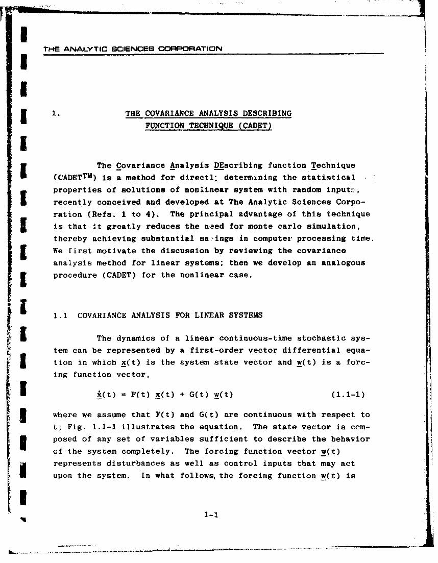
5 The dynamics of a linear continuous-time stochastic sys-
tem can be represented by a first-order vector differential equa-
l I tion in which x(t) is the system state vector and w(t) is a forc-
ing function vector,
A+ (t) =F(t) x(t) + G(t) w(t) (1.1-1)
where we assume that F(t) and G(t) are continuous with respect to
t; Fig. 1.1-1 illustrates the equation. The state vector is com-
* posed of any set of variables sufficient to describe the behaviorof the system completely. The forcing function vector w(t)
represents disturbances as well as control inputs that may act
upon the system. In what follows, the forcing function w(t) is
U -I'

THE ANALYTIC SCIENCES CORPORATION
Figure 1.1-1 Representation of the Continuous-Time
Linear Dynamic System Equations
P.ssumed to be composed of a mean or deterministic value b(t) anda random component u(t), the latter being comprised of elementswhich are uncorrelated in time; that is, u(t) is a "white noise"
process having the spectral density matrix Q(t). Thus w(t) isspecified by*
w(t) - b(t) + u(t)
Ea[wM) = NO)(112)L
E [ UMt u!T*T)] = Q(t) 6(t-T) [Similarly, the state vector has a deterministic component m(t)and a random part r(t); for simplicity mR(t) will generally becalled the mean vector. The state vector x(t), then, is described .
statistically by its mean vector and cov-eiance matrix,
x(t) = m(t) + r(t)(1.1-3)
M(t) = E [x(t)]
E denotes ensemble expectation, or average value; a super-script T denotes the transpose of a vector or matrix; 6(t-T)is the Dirac delta function.
1-2

THE ANALYTIC SCIENCES CORPOPATION
P(t) E [r(t) r'(t) (1.1m3)(Cont)
Henceforth, the time dependence of the variables w, b, u, Q, x,
m, r and P will not be explicitly denoted by (t). unless requiredfor clarity.
The differential equations that govern the propagation
of the mean vector and covariance matrix for the system describedby Eq. (1.1-1) can be derived directly, as demonstrated in Ref. 5,
[ to be
_ = F(t) m + G(t) b (1.1-4)
P = F(t) P + PF T(t) + G(t) QGT(t)
The firsL and second momeiats of the system response are completely
determined by integrating the above vector and matrix diffe.,,ntial
equations, Eq. (1.1-4), when the initial conditions, m(O) andP(O)*, are specified. The elements of m represent the effects of
deterministic initial conditions and biases due to determin-
istic system inputs (b 0 0). The diagonal elements of P arethe mean square values of the random components of the state
variables, and the off-diagonal elements represent thedegree of correlation between the random components of the
various state variables.
the Equation (1.1-4) provides a direct method for analyzing
S1 the statistical properties of x. This is to be contrasted withthe monte carlo method, where many sample trajectories of x are
calculated from computer-generated random noise and initial con-K. ditions, using Eq. (1.1-1). The moments m and P are then esti-
mated by averaging over the ensemble of trajectories generated inthe monte carlo procedure. Note that Eq. (1.1-4) leads to exact
The initial time can be taken to be t- 0 with no loss ingenerality.
1-3

THE ANALYTIC SCIENCES COR-PORATIO2N
solutions for m asad P, to within computer integration accuracy,
whereas the monte carlo method yields approximate solutions tor
any finite number of simulations. Furthermore, the mean and co-
variance equations need be solved only once over the time interval
of interest, whereas Eq. (1.1-1) must be solved repeatedly using
the monte carlo technique; consequently the direct analytical
method is not only exact, but is also generally the most efficient
technique for analyzing linear systems. With this observation as
motivation, we proceed to describe a methodology whereby the sta-
tistics of a nonlinear syste-i can be computed approximately using
recursive relationships similar in form to those of linear co-
variance analysis, Eq. (1.1-4); the monte carlo method is treatedin greater depth in Appendix C.
1.2 COVARIANCE ANALYSIS FOR NONLINEAR SYSTEMS
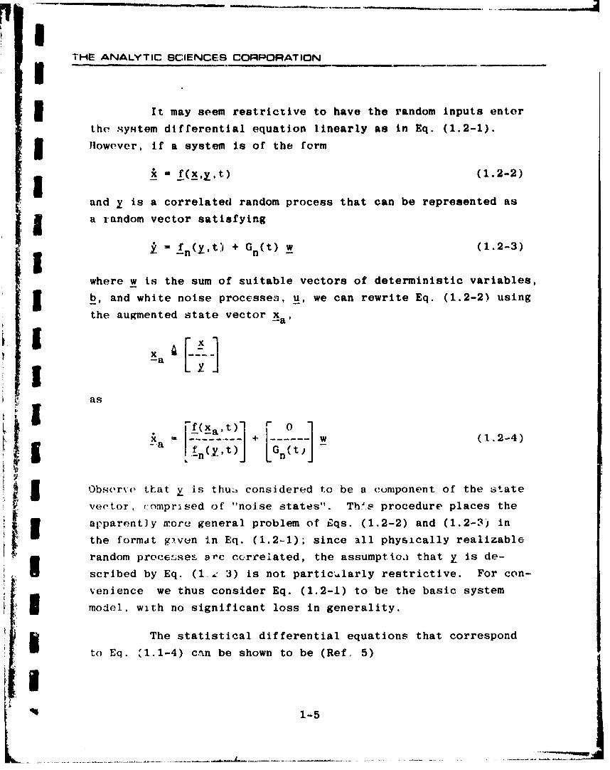
Th-e k.:onlinear counterpart of Eq. (1.1-1) treated in thispresentation is
f_- (_,t) + G(t) w(1.2-1)
Figure 1.2-1 depicts this equation. The input and state vectors I'are again characterized by the quantities b, Q and m, P, respec- vtively, given in Eqs. (1.1-2) and (1.1-3). V
R-11902w
++ NONLINEAR" "-FUNCTION
Figure 1.2-1 Nonlinear System Block Diagram
1-4
THE ANALYTIC SCIENCES CORPORATION
i It may seem restrictive to have the random inputs enter
the symtem differential equation linearly as in Eq. (1.2-1).
However, if a system is of the form
k - f(x,yt) (1.2-2)
and y is a correlated random process that can be represented as
a random vector satisfying
+ G (1.2-3)I • -~fn(y[,t) + n(t) w( . -)
where w is the sum of suitable vectors of deterministic variables,
I5 b, and white noise processes, u, we can rewrite Eq. (1.2-2) using
the augmented state vector xa,
asI . I ~~f(Xa't ' F 0 "
-- I--- -- " . .-----*. . . - w ( 1 . 2 - 4 )I ,~ -,a 4,•(Y,~ ~ntj
I 5.Obser\( that is thu:, considered to be a component of the state_ C
vector, rompri.sed of "noise states". Th,,Q procedure places the
apparently rror. general problem of iqs. (1.2-2) and (1.2-3) in
the format given in Eq. (1.2-1); since ill physically realizable
random proce;Jses a'ec correlated, the assumptio.a that y is de-scribed by Eq. (1 ,- 3) is not particuAarly restrictive. For con-
venience we thus consider Eq. (1.2-1) to be the basic system
model, with no significant loss in generality.
The statistical differential equations that correspondto Eq. .11.1-4) can be shown to be (Ref. 5)
Iq4 1-5

THE ANALYTIC 6CiENCES CORPORATION
tii E ý: 1(a.t)) + Ct(t)b Lf + G(t)_b (1.2-5)
SE [I !T] + 1[~T] + G;(t)QGT(t
The first equation is the direct analog of the mean differential {iequation of Eq. (1.1-4), since we observe that i' is simply F(t)rn
In the linear case. The nonlinear novariance equation can berepresented in the same format as indica t ed in Eq.'(1.1-4) by UL11defining the auxiliary matrix N,
NP E[xt)T](1.2-6)
Then Eq. (1.. -5) may be written asmi a + G(t)b L
(1.2-7)
P w NP + PNT + G(t)QGT(t)
The relation in Eq. (1.2-6) generally provides an explicit defi- [3nition of N,
N- E [f(•,)rT] Pr (1,2-8)
since P is usually positive definite* and thus a unique P- 1 -
exists.
The derivation of Eq. (1.2-5) is based directly on theprinciples of covariance analysis, Ref. 5. We observe, however,
Often the initial condition P(O) is only positive semi-.dofinite,in which case the pseudoinverse of P(O) could be used in Eq.(1.2-8).As shall be shown subsequently, Eq. (1.2-8) is only formal, in thesense that it is almost never used to evaluate N (refer to Eq.(1.2-10) and Seution 4.1).
1--6
rHE ANALYTIC SCIENCES CORPORATION
that. the vector f and matrix N defined in Eqs. (12-5) and (1.2-6)are Identical to the quantities which provide a minimum mean nquare
.rror uasi-linear approximation to the nonlinearity f(.,t). ItI ean be shown (refer to Section 4.1) that the approximation
f(xt) a f + N(x - m)
with f and N specified by Eqs. (1.2-5) and (1.2-6) yields the bestlinear approximrtion in the sense that
I e f(x,t) - f N(x- m)
satisfies the condition
E [eTse] - minimum
for any positive semi-definite matrix S. The intimate relation
between the well-established describing function theory (Ref. 6)
and Eq. (1.2-6) has permitted the rapid development of an approxi-S~mate nonlinear covariance analysis technique based on Eq. (1.2-7)il I eallv~d CADET -- the Covariance Analysis DEscribing Function Tech-
nique. Henceforth, we shall refer to if as the expectation vector
and N as the__=uasi-linear system dynamics matrix.
A
The quantities f and N defined in Eqs. (1.2-5) and (1.2-6)
must be determined before we can proceed to solve Eq. (1.2-7).* • Evaluating the indicated expected values requires knowledge of the
. .joint probability density function (joint pdf) of the state vari-r - ables. While it is possible, in principle, to evolve the n-dimensional joint pdf p(x,t) for a nonlinear system with randominputs by solving a set of partial differential equations known5 as the Fokker-Planck equation or the forward equation of Kolmogorov
(Ref. 5), this procedure is generally not practically feasible.3 The fact that p(x,t) is not available precludes the exnct solu-
tion of Eq. (1,2--7).
[ • 1-7

THE ANALYTIC SCIENCED COP"'".A• -_____l_
One procedure for obtairtnr an approximati, solution to
Eq. (1.2-7) 18 to assume the form of tk.v ,joit. prohability dten-
sity function of the state variables ir. Jrder to evaltvate f and N
according to Eqs. (1.2-5) and (1.2-6). Although it is possible
to use any joint pdf, all of CADET developMent to date has been
based on the assumption that the state variables are jointly
norinal; this choice was made because it is both reasonable and
c'onvenient.
While the above assumption is strictly true only for
linear systems driven by gaussian inputs, it is often approxi-
mately valid in nonlinear systems with nongaussian inputs, Al-
though the output of a nonlineailty with a gaussian input is
generally nongaussiar, it is known from the central limit theorem
that random processes tend to be made gaussian when passed through
low-pass linear dynamics ("filtered"). Thus, we rely on the
linear part of the system to insure that nongausslan noislinearity
outputs result in nearly gaussian system variables as Aignala
propagate through the system. By the same token, if there are HI.)
nongaussian system inputs which are passed through low-pass linear
dynamics, the central limit theorem can again be invoked to jus-tify the assumption that the state variables are approximately
jointly normal. The validity of the gaussian assumption for non-
linear systems with gaussian inputs has been extensively studied i
and verified; nongaussian random inputs have not been considered.
From a pragmatic viewpoint, the gaussian hypothesis serves
to simplify the mechanization of CADET significantly by permitting
each scalar nonlinear relation in f(x,t) to be treated in isola-
tion, with f and N formed from the individual random input describ-
ing functions (ridf's) for each nonlinearity. Since ridf's have
been catalogued in Ref. 6 for several classes of nonlinearities
encountered in a broad spectrum of practical problems, the

THE ANALYT'IC SCIENCES COROFXRA7IIN
Implimentation of CADET Is a straightforward procedure for the
analysis of many nonlinear systems. We also note that, under the
,3 gatussin assumption, the, random input describing functions can
"*I be calculated directly from the mean vector, m, and the covariance
matrix, P, of the system state vector, Thus, we write f and N
, In th .e fo'rm
3 f = f(m,P,t)5- -(1.2-9)
N = N(m,P,t)
As a corollary to the above observations, we have the result
(Ref. 7) that
IdN(m,P~t) - f (1.2-10)
Since calculating f is required for the propagation of the mean
I (Eq. (1.2-7)), it is generally much easier to employ Eq. (1.2-10)
than to eývaluate N directly using Eq.(1.2-6). Quasi-linearization
and the random input describing function are treated in somedtail in Chapter 4.
Relations of the form indicated in Eq. (1.2-9) permit
the direct evaluation of f and N at each integration step in the
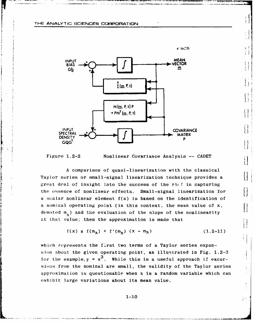
Ipropagation of m and P, is illustrated in Fig. 1.2-2. We note
that. the dependence of f and N on the statistics of the state vec-
tor is due to the existence of nonlinearities in the system. With-
out nonlinear effects, the propagation of the mean and covariance
g is "uncoupled," as in Eq. (1.1-4).
To demonstrate the ease witu ,hich CADET can be mech-3 anized under the gaussian assumption, we consider a low-order sys-
tem model for the missile-target intercept problem having a R'ngle
nonlinearity in Section 2.2. All of the steps involved in per-
forming statistical analysis via CADET are illustrated in detail.
1-9
THE ANALYTIC SCIENCES CORPORATION
BIASIi.
INPUT COVARIANCE
SPECTRALR e-
DENSITY MARIGQe
Figure 1.2-2 Nonlinear Covariance Analysis -- CADET
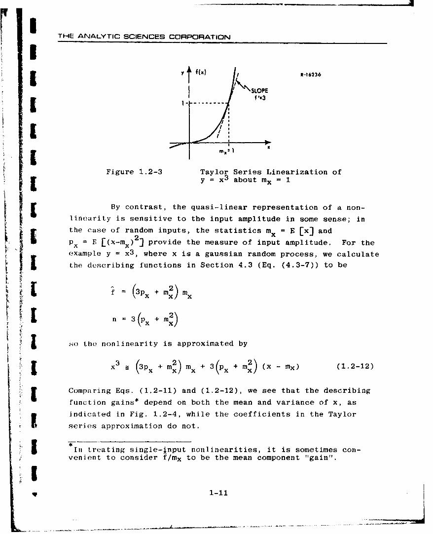
A comparison of quasi-linearization with the classical
Taylor series or small-signal linearization technique provides a Hgreat deal of insight into the success of the ri f in capturing
the essence of nonlinear effects. Small-signal linearization for
a scalar nonlinear element f(x) is based on the identification of
a nominal operating point (in this context, the mean value of x,
denoted mnx) and the evaluation of the slope of the nonlinearity
at that value; then the approximation is made that
f(x) = f(mx) + f'(mx) (x - mx) (1.2-11)
which represents the first two terms of a Taylor series expan-sion about the given operating point, as illustrated in Fig. 1.2-3for the example,y = x 3. While this is a useful approach if excur-
sio•,s from the nominal are small, the validity of the Taylor series
approximation is questionable when x is a random variable which can
exhibit large variations about its mean value.
1-10
THE ANALYTIC SCIENCES CORPORATION
IY R-16236
£ 1----------| 'I',
Figure 1.2-3 Taylor Series Linearization ofy = x3 about mx = 1
By contrast, the quasi-linear representation of a non-
linearity is sensitive to the input amplitude in some sense; in
the case of random inputs, the statistics mx = E [x] and2xPx = [(x-mx) ] provide the measure of input amplitude. For theexample y = x3 , where x is a gaussian random process, we calculate
the describing functions in Section 4.3 (Eq. (4.3-7)) to be
[n- ~ 3Px+m)x
~ [ n3(px~2)
so the nonlinearity is approximated by
x 3 3 + m2) x + 3(Px + m2) (x - mx) (1.2-12)• x x "
Comparing Eqs. (1.2-11) and (1.2-12), we see that the describing
function gains* depend on both the mean and variance of x, as
indicated in Fig. 1.2-4, while the coefficients in the Taylor
series approximation do not.
W *In treating single-Input nonlinearities, it is sometimes con-venient to consider f/mx to be the mean component "gain".
, 1-1

THE ANALYTIC SCIENCES CORPORATION
3t-11604
f/rnn
4
Quasi- Linearization for mX872 Quasi-Linearization for mX8l
Taylor Series Linearization obout mx, ITaylor Series Lioearization about mra 1
0 II 0 I
o 1 2 PX 0 1 2 PX(a) Mean Component Gain (b) Random Component Gain
Figure 1.2-4 Quasi-Linearization of y = x3 forUnity Input Mean
1.3 CONT[NUOUS/DISCRETE-TIME SYSTEMS
Preceding sections of this chapter have treated continuous-
time nonlinear systems; iLe., those that are governed by differen-
tial equations. However, in many practical applications, the sys- I
tem may include a digital computer whose operations are expressed
in terms of difference equations, as illustrated in Fig. 1.3-1.
Such a structure arises in missile guidance systems when digital
control laws are used to generate acceleration commands, for ex-
ample. In this section, equations are briefly developed for propa-
gating the mean and covariance of a nonlinear, mixed continuous/
discrete system. Systems which are wholly d~.screte can be treated
as special cases of the following discussion.
The equations of motion for a system of the type shown in
Fig. 1.3-1 are expressed in mixed differential./difference equation
format. In the continuous-time phase (between sampling instants,
tk, k = 1,2,....) the digital computer is inactive, and the statevariables of the system satisfy an equation of the form
1-12

THE ANALYTIC SCIENCES CORPORATION[1]
CONTINUOUS-TIME
RANDOM INPUTS[• -• DYNAMICS I
SAMPLER
k• DISCRETE-TIME
RANDOM INPUTS
Figure 1.3-1 An Example of a Mixed Continucus/Discrete System
f -t [+d [ M W J t k < - k+1S[-- - . .d. .l; -jS- ' - (1.3-1)-
Swhere• x (t) refers to the continuously-varying states in the sys-tem, and xd(t) is a collection of discrete-time states (e.g.,states in the digital computer) which remain unchanged betweenthe sampling times. Under the assumption that the state variablesare jointly normal, the statistics between sampling instants can
be propagated using a straightforward extension of the standardCADET equations (Eq. (1.2-7)) as follows:
f[cm,'Pt)] [G+(t)bc
K1 (1.3-2)I [Nm t !1 [GQGT -0jlc(m,P,t) + 0-'c ( m ,P t ) 0 ~ __[ ,, to ,o
0 0
i 't < t< tk -k+1
1-13

THE ANALYTIC SCIENCES CORPORATION
where N is the quasi-linear system dynamics matrix for the
(cfl. intious-time -dale( vnirinlibl,(', d(el'ined by
INL g E [f(x~t) rT]
which is of dimension (n0 x n); n is the total number of state
variables and n, is the number of continuously-varying states.
The continuous-time vector of white noise processes wc(t) is
described statistically by the mean vector bc and spectral
density matrix Qc as before (refer to Eq. (1.1-2)).
Observe that describing functions for a nonlinear time-
invariant function of gaussian discrete-time states alone need
not be evaluated continuously since the statistics of the
discrete-time states are constant in the interval tk < t < t
As a special case, if
f (x t) = 11 (xc't) + f 2 -d (1.3-3)
isthen N may be partitioned into two parts,c
IamPt c~cPctIc
'p'
m = ,P = Pd-Ccc 1 cdI~ (1.3-5)
_Md-cd Idd-
Sineo mnd and Pdd are constant during the continuous-time phase,
the matrix Nc2 is also constant.
At a sampling time, tk+1, the digital computer performs
a calculation which can be represented as a difference equation,
"1-14

THE ANALYTIC SCIENCES CORPORATION
X (tk+ [ ttk+l) 0
+ + (1.3-6)Wt (k+1) d (x(t k+l),t k+1) Gr k+l~k+1
where the superscript (+) denotes the new values of the state
variables just after a sampling instant.* I'he vector wk+l
I represents a discrete-time random quantity that can enter the
digital calculation as a result of sensor measurement noise,quanti-
zation, etc. It is assumed that wk+1 has a mean of bk+l and a
covariance matrix Qk . Observe that in Eq. (1.3-6) xc remains
unchanged, since variables that satisfy differential equations
cannot change instantaneously in time. Situations where it is
reasonable to assume that E continuous-time variable can change
"almost instantaneously" as a result of a digital operation can
be treated by decomposing that variable into components that are
strictly continuous (an element of xc) and digital (an elementS sori t he codiio thatta
of X), so the condition that x,(t+) = xc( t k+l) represents no
loss in generality.
Because the mean and covariance of x and xd at t are-c an tdk+l
| known from Eq. (1.3-2), the expectation vector Sd and quasi-linear
system dynamics matrix Nd corresponding to Ld in Eq. (1.3-5) can
I !be evaluated. Thus we can rewrite the discrete-time part of Eq.
(1.3-6) approximately asdtk+1) • d+Nd •(kl -t +l Gk+l~k+1
(td + N (t k+1) rn(tk+l)J wkly~ (1.3-7)
From Eq.(1.3-7) it follows that the mean and covariance of the sys-tem states just after the discrete-time calculation are given by
The discrete-time operation actually takes place between tk+1 andtk+1 + c. In this discussion it is assumed that c is negligible incomparison with the time-scale of the continuous-time dynamics,although finite computational delays can be treated in a straight-forward manner.
q 1-15

I HF ANALY I I( t ;( ;Ir N•LS CORPORATION
Cn-c tk+1) = nc(tk+1)
=-d
md(tkl f
P(t t+l )=dt_. t l) _,,NT + 0 G + ~ +G +
ltk+1) - (t=)N±dOl~k1 L0'1 G [ Gk+lQ:+ IGk+1]d Lo (1.3-8)
After evaluating Eq. (1.3-8), m(t+ and P(t are the. _ k+1)adP k+l)aete nta
conditions for propagating the mean vector and covariance matrix
over the next continuous-time phase using Eq. (1.3-2). Thus by
alt,,rnately implementing the continuous-time and digital mean
vector and covariance matrix propagation equations, Eqs. (1.3-2)
and (1.3-8), the performance of a nonlinear system described by
a mixed differential/difference equation can be evaluated.
The developments discussed in this chapter provide the
neces(,,ary tools for analyzing the performarice of a broad class of
nonlinear systems with random inputs. The efficiency realized byCAI)ET has made it an attractive technique for performing sensi-
tivity studies and investigations of the impact of nonlinear
effects on the accuracy of tactical missile guidance systems; it
is anticipated that CADET will prove to be equally powerful in
treating other nonlinear systems.
1-16
THE ANALYTIC SCIENCES CORPORATION
52. CADET APPLICATION: SIMPLE ILLUSTRATIONS
In this chapter we demonstrate many of the details that
are involved in the application of CADET to a practical probleminvolving the statistical evaluation of the performance of a non-linear system with random inputs. Simplified formulations of the
5 missile-target intercept problem are treated, with guidance modulesthat are either analog or digital; the corresponding CADET equa-5 tions are obtained; and their solution -- to establish the evo-
lution of the system variable statistics during a given scenario -
is outlined in computer flow-chart format.
5 2.1 MISSILE-TARGET EQUATIONS OF MOTION
5 This sect ion treats -,he basic differential equations
describing the motion of a tactical missile and a target to be
g intercepted. In subsequent sections, examples of two types of
S guidance modules are considered -- continuous-time (analog) and
discrete-time (digital) -- to provide -the basis for detailing the
~ K NDET methodology, both for systems represented entirely by dif-~rential equations and for systems described by mixed differential/5 difference equations. In order to obtain a system model which is
simple enough to permit a clear presentation of the step-by-step
procedure entailed in the use of CADET, we reduce the planar
missile-target intercept problem to its bare essentials. Chapter 3provides a more detailed discussion on modeling the missile-target
~ U intercept problem; here we present only a summary of the required
dynamic equations.
U The ecoordinate frame and the basic variables are por-trayed in Fig. 2.1-1. Here we consider variations about a head-on
2-

THE ANALYTIC SCIENCES CORPORATION
y-AxIS R-1192It, t1 )S-AXIS
VEOC0) VELOCITY
.,ZVt E-Ut )VELOCITY ACLITO
ACCELERATION iOt tt
6'h) ARGIT TRAJECTORYMISSILE TRAJECTORY __NAI
•L. ..... -AXISORIGINAL ORIGINAL LINE-OF-SIONT (LOS) ORIGINAL (too)MISSILE TARGETPOSITION POSITION
Figure 2.1-1 Missile-Target Planar Intercept Geometry
intercept, i.e., the missile lead angle, 01, and target aspect
angle, 0 a, are assumed to be small. For the purpose of illustra-
ting the mechanization of CADET, we make the followirg approxi-mations based on small-angle assumptions:
9 The down-range separation, x, and missile-target range, r, are deterministic, givenapproximately by
x(t) a r(t) i (vm+vt )(T-t)
(Vm+vt ) tgowhew T is the nominal terminal time (time of
intercept), tgo is the time-to-go, and vm andvt are the constant missile and target velocitymagnitudes, respectively.
e The lateral or cross-range separation, y, isdetermined by the missile and target lateralaccelerations, am and at respectively, as 4.nEq. (3.5-14)
Y at am (2.1-2)
* The autopilot and airframe dynamics are repre-sented by a linear plant, modeled by a transferfunction with a single dominant pole at s=-l/T,
2-2
I .~ -

ITHE ANALYTIC SCIENCES CORPORATION
followed by an ideal limiter, to model the air-"I frame saturation effect. Thus the unlimited
missile lateral acceleration 14 satisfies theI •differential equation
Im* + Im " I ac (2.1-3)
where ac is the acceleration command generatedby the guidance module, and the limited value,5i am, is given by
X m< amaxam = f(m) - (2.1-4)ami amaxSign( Im), 'a"m I > amax
9 The target acceleration, at, is the sum of adeterministic variable and a band-limitedgaussian process satisfying
i t + Wt at u w(t) (2.1-5)
where wt is the target maneuver bandwidth. TheI random input w is described by
E [w(t)] - b(t)
E [(w(t)-b(t))(w(T)-b(T))] = q(t) 6(t-T)
where b is the deterministic component of theinput and q is the spectral density of the whitenoise process, w - b.
Given the preceding simplified equations of motion, we complete
the missile-target intercept model by considering simple examples
of the two basic classes of guidance modules: continuous-time and
32.2 THE CONTINUOUS-TIME CASE: PROPORTIONAL GUIDANCE
The acceleration command dictated by the classical pro-3 portional guidance law (refer to Section 3.5.1) is given by
ac n' vc (2.2-1)
I,2S~2-3
-------------------------------------
2
THE ANALYTIC SCIENCES CORFPORATION
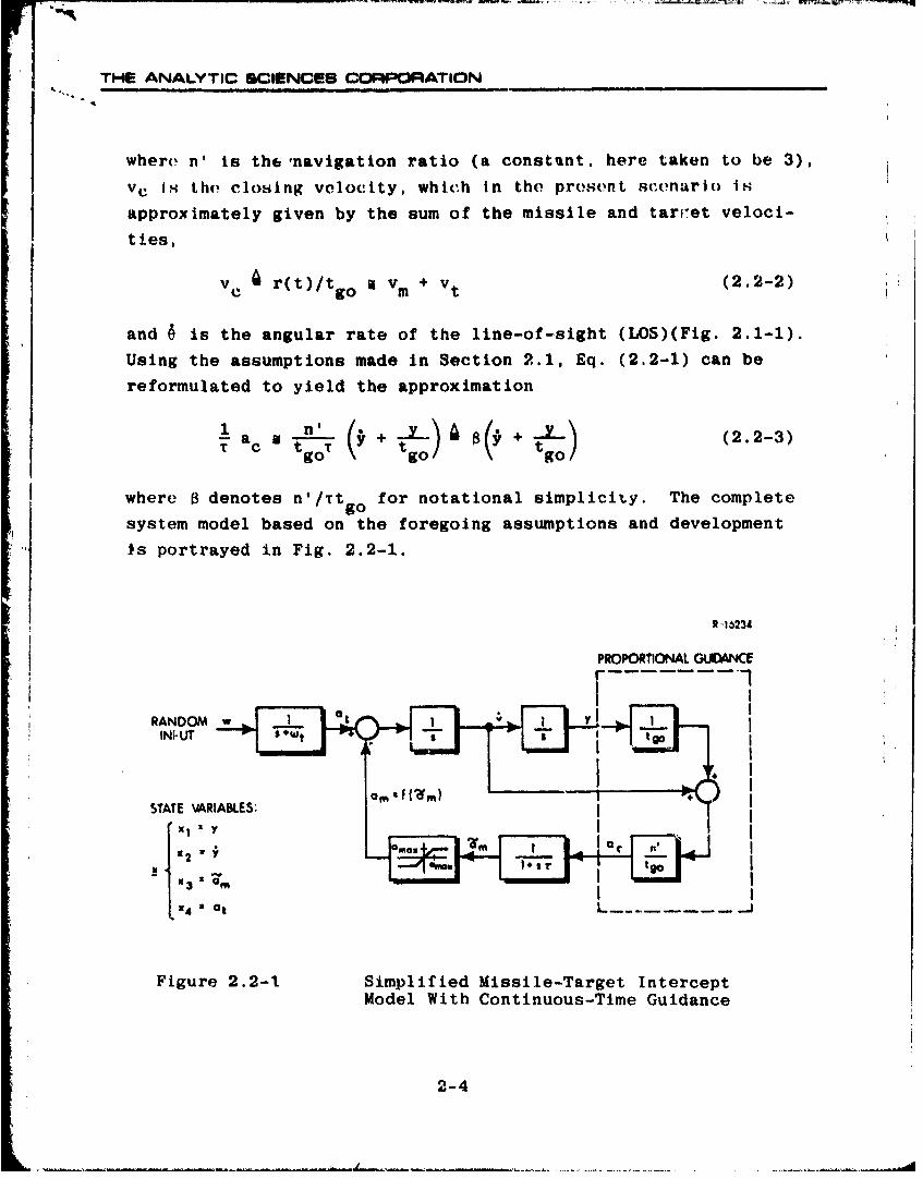
where n' is the-navigation ratio (a constant, here taken to be 3),
vC Is the closing velocity, which in the present scenario Is
approximately given by the sum of the missile and tarret veloci-
ties,
v r(t)/t i v + v (2.2-2)Sgo m t
and 4 is the angular rate of the line-of-sight (LOS)(Fig. 2.1-1).
Using the assumptions made in Section 2.1, Eq. (2.2-1) can be
reformulated to yield the approximation
a t In + + (2.2-3)aT g T tgg togo)
where 8 denotes n'/Ttgo for notational simplicity. The complete
system model based on the foregoing assumptions and development
$s portrayed in Fig. 2.2-1.
R -1,234
PROPORTIONAL GUOINCE
INW" T $ +Wt g
STATE VARIABLES: M
uuou at r
" X3 a om m maIIN4 at
Figure 2.2-i Simplified Missile-Target InterceptModel With Continuous-Time Guidance
2-4
THE ANALYTIC SCIENCES CORPORATION
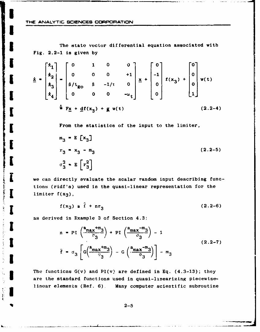
3 The state vector differential equation associated with
Fig. 2.2-1 is given by
I 11 0 1 0 0 0- 0-
2 0 0 x + f(x 3 ) + w(t)*3 O/t ° B -1/T 0 0 0S• •t 1
L*4J 0 0 0 _W tj L0J J
[ Fx + df(x 3 ) + I w(t) (2.2-4)
From the statistics of the Input to the limiter,
m 3 - E Ex3 ]
r•3 a x 3 - m3 (2.2-5)
2)e o3r uEd i t3
we can directly evaluate the scalar random input describing func-tions (ridf's) used in the quasi-linear representation for the
•: limiter f(x3),
b. I f(x3 ) A f + nr 3 (2.2-6)
as derived in Example 3 of Section 4.3:
n Pn-PT ( ma +m3 ( amxr3(2.2-7)
fa 3 [G~aa+3 G (aain) m3
* IThe functions G(v) and PI(v) are defined in Eq. (4.3-13); they
are the standard functions used in quasi-linearizing piecewise-
linear elements (Ref. 6), Many computer scientific subroutine
2-5

THE ANALYTIC SCIENCES CORPORATION -
pa('kaLg(oH have avatlRblP the subroutine "EqRF(v)", in whichcase. ii
PI(v) 1 + ERF
1(2.2-8)
G(v) - vPI(v) + e
permits direct calculation of f and n. Given the two constituents
of the quasi-linear representation of the limiter indicated inEqs. (2.2-6) and (2.2-7), we substitute into Eq. (2.2-4) to get
f Fm + df
N.0 1 0 (2.2-9)S0 0 -n 1 i
N"
0/tgo 0 -1/T 0
0 0 0 _t
Finally, from the input statistics, b and q, the dif- [Jferential equations and initial. conditions that approximatelygovern the propagation of the state vector deterministic com- Hponent ("mean") and covariance matrix are givetr by Eq.(1.2-7):
_ + g b; m(0) - MO
(2.2-10)
Te AETNP + PNT + q; P(C) - P0
The CADET methodology utilizes the preceding relations to deter-mine the time histories of the mean vector, m, and covariance
matr.x, P, over the duration of an ensemble of engagements
(0 < t < r). Any standard numerical integration technique maythen be uccd to solve Eq. (2.2-10).' The structure of a computer
2-6

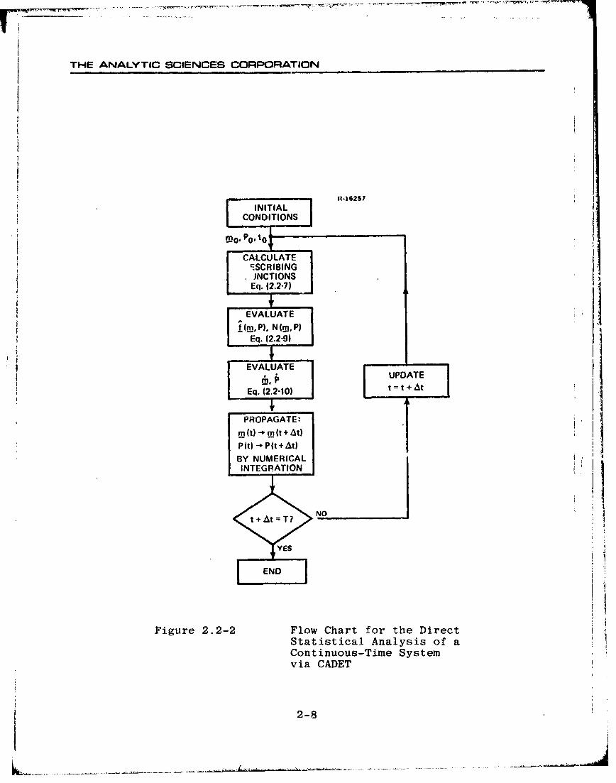
THE ANALYTIC SCIENCES CORPORATION
ii program to (carry out the CADET analysis of tactical missile per-
formance is indicated in Fig. 2.2-2.
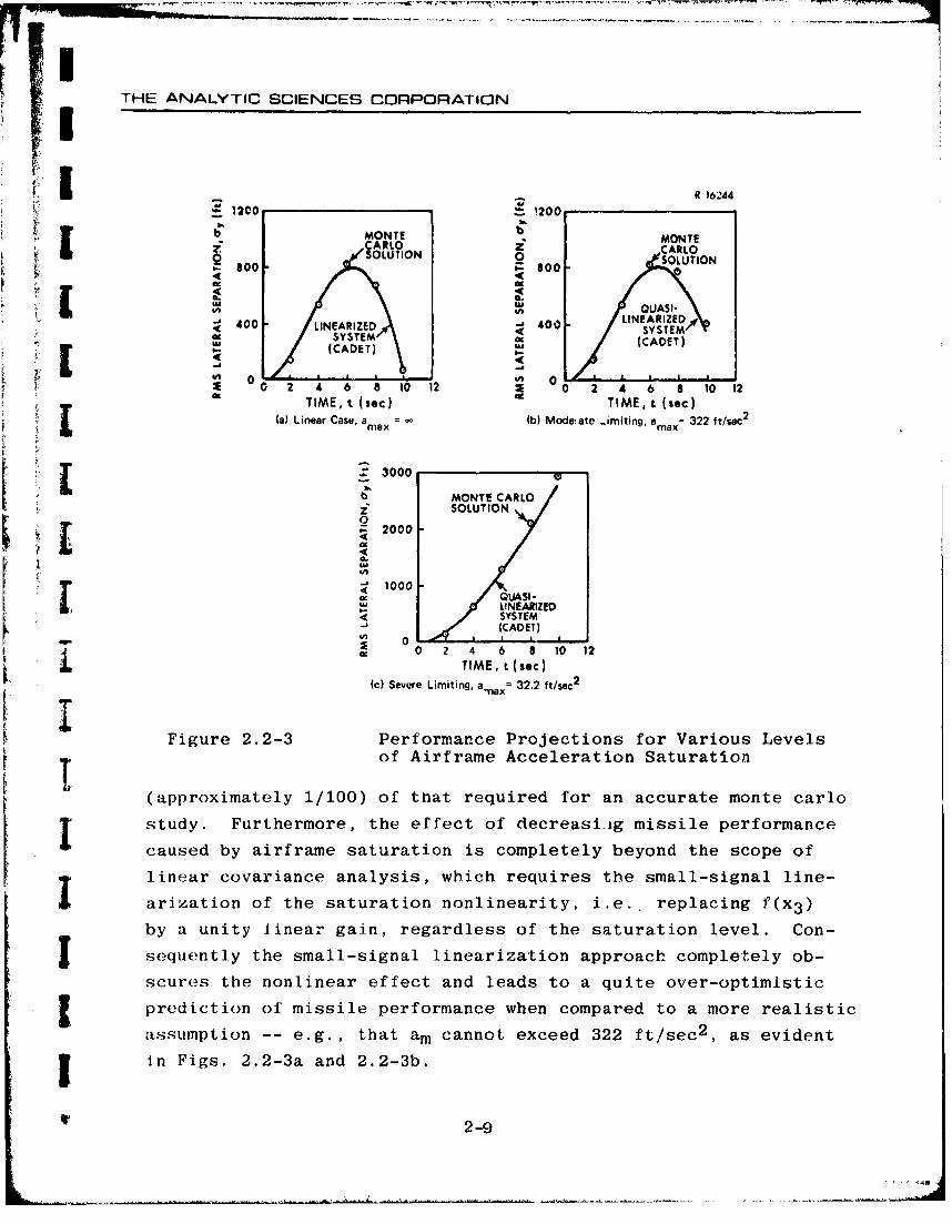
I The results of a CADET and monte carlo statistical anal-
ysis of the performance of the preceding missile guidance system
(obtained from Ref. 1) are depicted in Fig. 2.2-3. Since the rms
lateral separation between the missile and target is of primary
importance in assessing tne ability of the missile to intercept
the target, only that variable is portrayed. The white noise in-
put spectral density, q, was chosen to be a constant yielding anI 2rms target lateral acceleration of 160 ft/svc , the bandwidth w
was assumed to be 1 rad/sec, and the autopilot time constant T
was taken to be 1 sec. All initial conditions (i 0 and P0 ) were
zero.
This missile performance study considered three levels
of "tirframe saturation. In Fig. 2.2-3a, the linear case cor-
responding to an infinite acceleration command limit is shown;
here, CADET reduces to the standard linear covariance analysis
(Section 1.1) which is exact, and the 200-trial monte carloanalysis provides an adequate approximation to this result. For
I the study of Fig. 2.2-3b, the restriction that the missile lateral
acceleration cannot exceed 322 ft/sec 2 leads to a five-fold in-J crease in y at the terminal time, here taken to be 10 sec; theSyCADET and monte carlo approximate solutions are in good agree-
I ment. Even in the case where the missile lateral acceleration
constraint is very severe (amax = 32.2 ft/sec 2 ), causing a further
1. ,rge decrease in missile capability as shown in Fig. 2.2-3c, the
CADET solution is verified by the monte carlo analysis.
Thus we observe that the direct statistical analysis via
CADET, implemented according to Fig. 2.2-2, quite accurately cap-
tures the effect of a significant nonlinearity in the missile-
target intercept problem. This investigation is performed withan expenditure of computer time that is a small fraction
22-7
THE ANALYTIC SCIENCES CORP•RATION
i 11-16257I INITIAL t165
CONDITIONS
CALCULATE 1=.SCRIBING 1
A JCTIONS
¶ Eq. (2.2-7) j
j EVALUATEf(n, P). NI(, P)
Eq. (2.2-9)
EVALUATE U PDATE
Eq. (2.2-10) t t + At
PROPAGATE:m (t) -*m(t +A0t
P(t) - P(t +At)
BY NUMERICALINTEGRATION
NOt+At=T? N
YES
END
Figure 2.2-2 Flow Chart for the DirectStatistical Analysis of aContinuous-Time Systemvia CADET
2-8
THE ANALYTIC SCIENCES CORPORATION
1It 16244-- 120}0 - 200 -
b MONTE MONTESCARLO ZCARLO
L OL600 600 &SOLUTIONIlk g oo o
Q OLJTIO 400LINEARIZED~A t 400 LINEARIZED 0 -5STE0'SYSTEM C(CADET)[ ~ (CADET)
0 2 4 6 a 10 12 a 0 2 4 6 8 10 12TIME, t (sac) TIME, t (sec)
(a) Linear Case, a = Ib)Mode:ate .imiting, am = 322 ft/sec2
max max
3000MONTE CARLO•.• " SOLUT•
0 SOLUTIONS2000
10004 6 O 0 1
X 0
Figure 2.2-3 Performance Projections for Various Levelsof Airframe Acceleration Saturation
(approximately 1/100) of that required for an accurate monte carlo
study. Furthermore, the effect of decreasi.og missile performance
caused by airframe saturation is completely beyond the scope of
linear covariance analysis, which requires the small-signal line-
arization of the saturation nonlinearity, i.e. replacing f(x 3 )by a unity linear gain, regardless of the saturation level. Con-
sequently the small-signal linearization approach completely ob-scures the nonlinear effect and leads to a quite over-optimistic
prediction of missile performance when compared to a more realistic
assumption -- e.g., that am cannot exceed 322 ft/sec 2 , as evident
in Figs. 2.2-3a and 2.2-3b.
2-9

• -- rr Tl ,- -,r r. r -
THI ANALYTIC SCIENCES CORPORATION
2.3 GUIDANCE SYSTEMS WITH DIGITAL DATA PROCESSING
In some guidance systems, discrete-time measurements ofcertain system variables are made available to a computer fordata processing purposes; acceleration commands are then calcu-
lated (in an on-line mode by use of a suitable algorithm) which Iiare used to control the missile. In this presentation, we assume
that the available signal is a noisy sampled measurement of LOS
angle, 0, so we have the sequence of values given by
Zk = ek + Vk, k = 1,2,... (2.3-1)
at the sampling instants, tk =kT, where is the sampling .1period. The zero-mean white noise sequence, v k, is quantified i
by its variance
~2 - ~ 2] (2.3-2)V Lk
Generally, the random effects modeled by this sequence include
external inputs (e.g., jamming) and measurement error. In light
of the small angle conditions, we use the approximation
a y/r A xl/r (2.3-3) f
where r is deterministic, gJven by Eq. (2.1-1), and x 1 is thestate variable representing y, Fig. 2.2-1.
Based on the information prov±ded by the measurement
sequence zk, the computer algorithm is often of the form
Vd(tk) = Fdk ?d(tk) + kkZk (2.3-4)
2-10
Id
THE ANALYTIC SCIENCES CORPORATION
(cf. Section 3.5.2 for the design of a guidance modulo hisod on
the Kalman filter and optimal cotrt.'ol tlhory) wltl' %d i., (ho
vector of digital states, comprised of variables which are stored
in memory and up-dated according to Eq. (2.3-4) as each new mea-
surement zk is made and processed. The matrix Fd,k and vector
_k, which may vary from one digital operation to the next, are
specified by the filter algorithm. The difference equation,
Eq. (2.3-4), in combination with the initial condition Xdo deter-
mines the time-histories of xd"
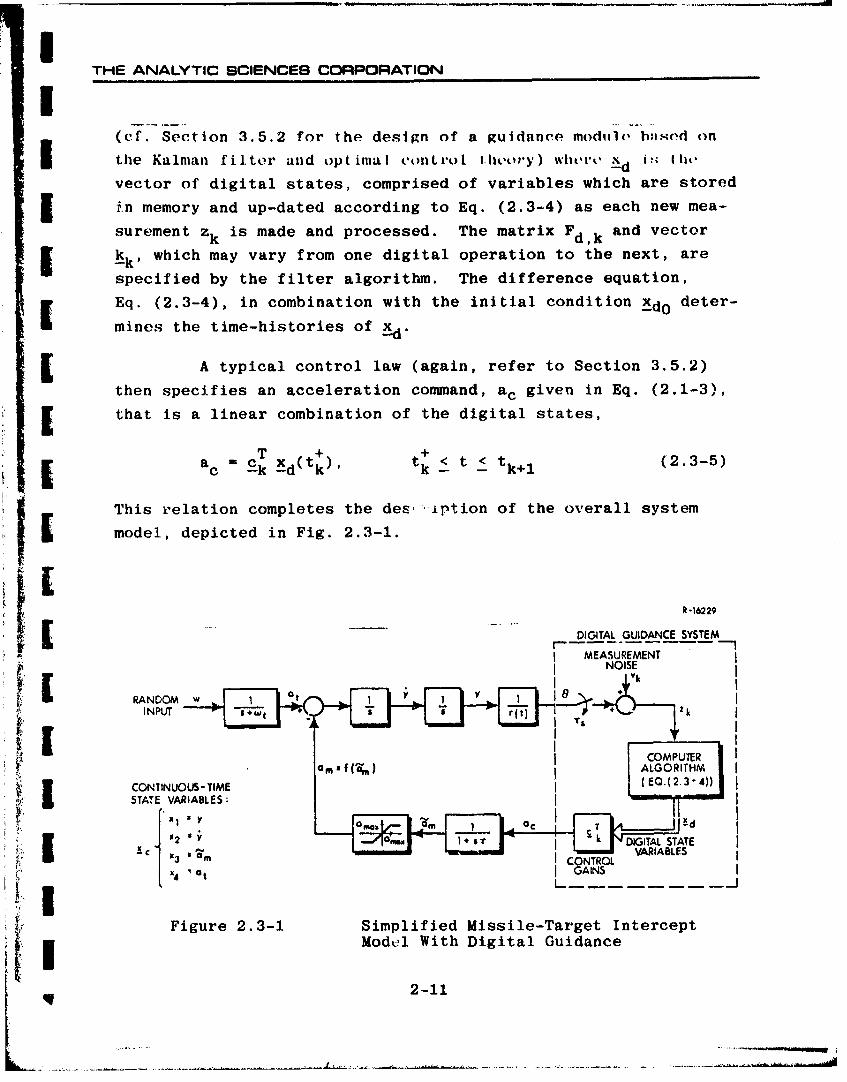
j A typical control law (again, refer to Section 3.5.2)
then specifies an acceleration command, ac given in Eq. (2.1-3),
i that is a linear combination of the digital states,
T + +ac ' -k xd(tk)' tk < t < ttk+1 (2.3-5)
This relation completes the des; iption of the overall system
j model, depicted in Fig. 2.3-1.
R-16229
DIGITAL GUIDANCE SYSTEM
E MEASUREMENTNOISES, --vk
i CONTINUOUS- TIME E 0. (2. -" "'))STATE VARALES : _
/x3 a m ICONTROLSx4 - at I GAINS
Figure 2.3-1 Simplified ssile-Target InterceptModel With Digital Guidance
2-11
L, _ _
THE ANALYT".. SCIENCES CORPORATION
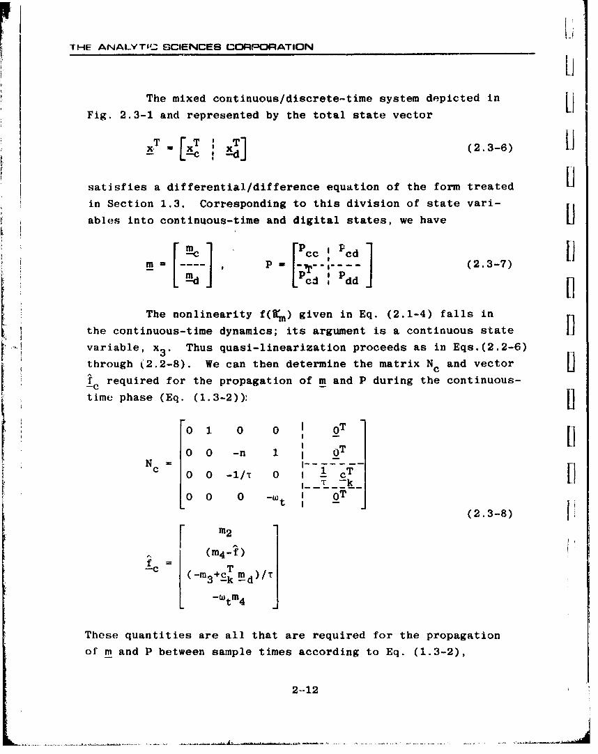
The mixed continuous/discrete-time system depicted in
Fig. 2.3-1 and represented by the total state vector
HeT - (2.3-6) Lsatisfies a differential/difference equation of the form treated Hin Section 1.3. Corresponding to this division of state vari-
ables into continuous-time and digital states, we have U
rn= P - (2.3-7)
Pd , Pdd
The nonlinearity f(sm) given in Eq. (2.1-4) falls in
the continuous-time dynamics; its argument is a continuous state ivariable, x 3 . Thus quasi-linearization proceeds as in Eqs.(2.2-6)
through (2.2-8). We can then determine the matrix Nc and vectorfC required for the propagation of m and P during the continuous-time phase (Eq. (1.3-2)):
"0 1 0 0 0 T
0 0 -n 1 0TN 0 -1/T 0 1 cT H
T -k
L -
(2.3-8)m2
(4-f)f T- (m _m+ckT md)/T-ctm
These quantities are all that are required for the propagation
of m and P between sample times according to Eq. (1.3-2),
2-..12
THE ANALYTIC SCIENCES CORPORATION
Ib
~in[3, [~3b(2.3-9)
I +, -i N,,K 4--0] q
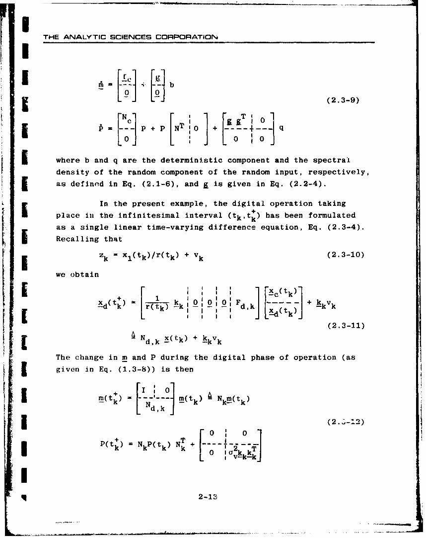
i where b and q are the deterministic component and the spectral
density of the random component of the random input, respectively,
as definod in Eq. (2.1-6), and g is given in Eq. (2.2-4).
In the present example, the digital operation taking
place in the infinitesimal interval (tk,tk) has been formulated
as a single linear time-varying difference equation, Eq. (2.3-4).
* Recalling that
zk = xl(tk)/r(tk) + vk (2.3-10)
we obtain
SI c(tk)
EI ( I I +
[,r.; k) k,_ , ,o Fd -k. k,[2i- /• k - -I -, - I '• /x (t ) -kk
(2.3-11)
d,k x(tk) + kkv
The change in m and P during the digital phase of operation (as
given in Eq. (1.3-8)) is then
P(tk) k Nk-P(tk N- k + ---- 1 2 Tkm( -)-0 10 k
S~2-13

THE ANALYTIC SCIENCES CORPORATION
Implementation of the CADET equations giveii above (Eqs. (2.3J-9)
and (2.3-12)) is portrayed in computer flow-chart format in IFig. 2.3-2.
We observe that thiý difference equation satisfied by
the digita~l states is lineav time-varying, so the matrix Nd(Eq. (2.3-11)) contains no describing functions. If it is neces-
sary to include nonlinear effects in the discrete-time portion of
the system model, one must evaluate appropriate random input
describing functions to be substituted in the vector fand
matrix Nd (Eq. (1.3-7)); some added complexity is entailed in
this case.
The examples 'liven in Sections 2.2 and 2.3 illustrate
the fundamentals involved in the application of CADET to pro-vide assessments of the performance of a tactical missile repre-
sented by a simple low-order system model with one significant
nonlinear effect. CADET has been successfully applied to system
models of considerably higher order and complexity (refer, for
example, to Table 5.1-1). The flow charts sho~wn in Figs. 2.2-2 '
and 2.3-2 accurately reflect the methodology used in the more
complex problems.
2-14

:'HE ANALYTIC SCIENCES CORPORATION
I
INITIALCONDITIONS
too. Po. to| I ~CALCULATE!•
I DESCRIBING NO -t.? "I FUNCTIONS t a T "?
S~~~q. (2.2-7) ! i"
Eq (238)E. (2.3-,4)
I
I
I
I
IFigure 2. Flow Chart for the DirectStatistical Analysis of a MixedContitnuous/Discrete-..Time SystemI via CADET
q (2-15
~~~~~q (2.3kU- 6)- -
THE ANALYTIC SCIENCES CORPORATION
3. MODEL DEVELOPMENT FOR THE
MISSILE-TARGET INTERCEPT PROBLEM
This chapter presents mathematical models which describe
various subsystems required in treating the general missile-
target intercept problem. The material included here summarizes
the nonlinear effects that have been treated in past CADET appli-
r cations (Refs. 1 to 4). The aims of this presentation are to aidI future users of CADET in analyzing tactical missile performance,
and to provide some guidance in modeling analogous phenomena that
may occur in the simulation of other nonlinear systems with ran-
31ELEMENTS OF THE MODEL
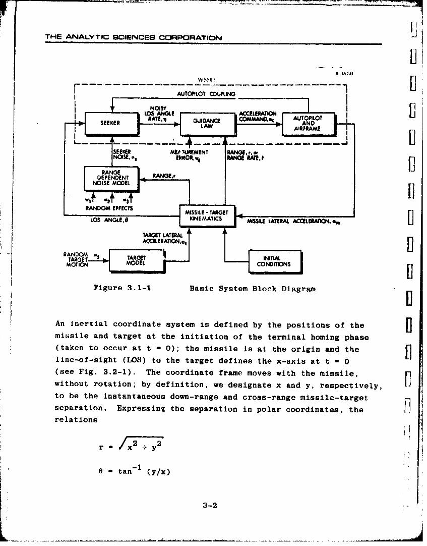
The overall interconnection of the subsj'stems which
~ [comprise the missile-target intercept model is indicated inFig. 3.1-1. The principal variables are shown as outputs of the
~~ appropriate blocks, and random disturbances are denoted w.
Detailed models underlying each input-output relationship are
~, 7 given in subsequent sections of the chapter. Observe that the
~ I models developed here are of considerably greater realism than
those used in t~ie illustrative examples of Chapter 2, alth~ough
~ the basic closed-loop guidance system is of the same structure.
3.2 THE MISSILE-TARGET KINEMATICS MODEL
The missile-target engagement presented here is restricted
~ to the terminal homing phase in a planar intercept configuration.
3-1
THE ANALYTIC SCIENCES CORPORATION 1<[J1
L 0 A G E C E L R T INAU T O P IL O T C U L Nse~e •RATEq I GUIDANCE COTANOcL"inT "IAND
RANDAESEPENDENT RNWLWMEN 1A]oo
LOS ANGLE, A9 E AERL'KINEMATICS MISILE LATERAL ACCELEATlON.o LIRANDGM eFeCS ISIE EARETr
MOTION MODEL OIN
Figure 3.1-1 Basic System Block Diagram
An inertial coordinate system is defined by the positions of the
missile and target at the initiation of the terminal homing phase l
(taken to occur at t - 0); the missile is at the origin and the [line-of-sight (LOU') to the target defines the x-axis at t " 0 L(see Fig. 3.2-1). The coordinate frame moves with the missile, p]without rotation; by definition, we designate x and y, respectively, lto be the instantaneous down-range and cross-range missile-targetseparation. Expressing the separation in polar coordinates, the 11]relations
W I xW 2 W3 y
-1,
W-2 W2-2 IeMISStLE -T(y/x)
LO AGE. INMTIS MISLELTEA ACLEA2Oe
ITHE ANALYTIC SCIENCES CORPORATION
I define the instantaneous range and LOS angle of the target. Thaangles e0 (missile lead angle) and 8 (target aspect angle) spe-
cify the orientation of the missile and target velocity vectorswith respect to the x-axis, and eva defines the direction of the
i missile acceleration vector with respect to the velocity vector;by convention, 80, 8a and eva are positive in the directions de-I fined in Fig. 3.2-1.
i y-AXiS R-'-"2
y -AXISS
v-AXIS (tat,)
_ (tIo) VELOCiTY_•VELOCITY A(ELEUATION
ACCELERATION -'m °-s t
e---,,--, u- AXIS
m/MI$O1)RA •TO TARGET TRAJECTORY
-'... •- \ - -NORIG,,NAL OIGINAL LINE-OP.SIONT (Los) oRiGNAL. ( t.o)
MISIL TARGETt
[O POSITION POSITION
Fig~are Z.2-1 Target-Missile Planar[ Intercept Geometry
I In derivini the equations of motion, it can often beassumed that the mi•.i•le and target velocity vector magnitudes
are constant, or, equivalently, that the missile and targetacceleration vectors are normal to the velocity vectors (e.g.,Ivais 90 degrees in Fig. 3.2-1). This •nidition, which neglects
heeffect of drag, is representative of many miE~ile-target3 engagement situations during the critical last few seconds.Under this assumption, the lateral acceleration of either vehicle
-A I
9 3-3
(tat,),
THE ANALYTIC SCIENCES CORPORATION
prodU(c,, it rotuation or tho corrosponding veloci'ty vector, givenby
£ Vm M(3.2-1)
6a -t at
The equations describing the relative motion of the target are Udetermined by projecting the velocity vectors onto the axes
shown in Fig. 3.2-1; in terms of the velocity magnitudes vm and vt, I.
-- V"m cos ( - vt cos (ea)(3.2-2)I •--vm sin ( + Vt sin (8 a6
Equation (3.2-2) represents the essential nonlinearities inherent
to the missile-target kinematic relationship; the overall kine- Umatic equations are portrayed in block diagram form in Fig.3.2-2.
1-11593
ott.
Vt I ts6
,, ,o I.! '="• RANGE
Figure 3.2-2 Block Diagram Formulation of
Missile-Target Kinematics
3-4

THE ANALYTIC 9CIENUES CORPORATION
3 In situations where drag effects are not negligible, the
missile velocity vector magnitude will vary with time (according
Ito a nonlinear differential equation) due to the fact that a is
not normal to vM ( 9 va 0 90 deg). Thus vm must be treated as a
state variable and the velocity vectnr rotation is given by the
fl nonlinear relation
IaV - --sin (0va) (3.2-3)m
SThis case is discussed in greater detail in Sectiotle 3.4.
3.3 THE TARGET MODEL
The model representing the target behavior is based on
the assumption that the target velocity has constant magnitude
with a direction described by the aspect angle, 0a, shown in Fig.
3.2-1. The aspect angle is determined by the target lateral
S[ accoleration, at, as indicat-d in Eq. (3.2-1). A commonly-used
target maneuver model represents target lateral acceleration asa correlated gaussian process derived from a gaussian white roiseinput by one stage of low-pass filtering. In differential equa-
S;tion formulation, we have*
it = -Wt at + w5 (3.3-1)
This relation and the equivalent low-pass filter representation
are depicted in Fig. 3.3-1
By adjusting the values of target maneuver bandwidth,
Wt, and rms level, oats a wide range of target maneuver charac-
p. I teristics can be represented. The instantaneous target maneuver
*The five white noise inputs to the system are simply denotedwj, j - 1,2,...,5, to correspond with Fig. 3.1-1.
3-5

THE ANALYTIC 3CIENCEB CORPORATION
- --- i i3i--11 i_
(a ifforentiaI Equation Re~resntetion
"w- at
iii
1b) rransfw Function Fornmulallon
Figure 3.3-1 Band-Limited Gaussian Noise Modelfor Target Lateral Acceleration
rms level is determined by the spectral density, q5, of the rar-
dom input w5 and the initial condition on Gat; for example, if
q5 is constant and
_.!5i
E [at(o)1 _ q (3.3-2)2 t
then the rms level of the target acceleration is constant through-
out the engagement,
Gat _ /2w (3.3-3)
It is important to note that the autocorrelation func-
tion and the corresponding power spectral density for a poisson
square wave -- i.e., a square wave that switches between ±Datft/sec2
with random poisson-distributed switching times having an average
of Wt/ 2 zero-crossings per second (Ref. 8) -- are identical to
those of the above gaussian process, although the associated proba-
bility density functions are quite different. The poisson model
3-6
THE ANALYTIC SCIENCES CORPORATION
is often used to represent target evasive or "jinking" maneuvers.The poisson square wave can only take on values of ± Oat, so at
any given time its probability density function (pdf) consists of
impulses with a weighting of 0.5 at plus and minus Oat, whereas
the above markov process is assumed to have a gaussian amplitude
distribution. Therefore, the response of an amplitude dependent
nonlinear operator could be quite different whren driven by each
of these two signal forms. However, if the random square wave is
passed through a narrow-band filter or integrator, its pdf would
experience broadening due to the filter's finite bandwidth. In
the case of an integrator, for example, the resulting wave shape
would be a series of linear segments of constant slope. By appli-cation of the central limit theorem, as discussed in Ref. 8, the
H1 distribution of the output of a linear subsystem approaches the
gaussian density function as the number of stages of filtering it
represents increases. In this case, the relative target position,
given by x and y in Fig. 3.2-2, are of particular interest in
assessing the performance of a tactical missile; these variables
are two integrations removed from at. Thus, although the poisson
square wave may in some situations be a more realistic target
maneuver model, we take advantage of the statistical similarity
of the gaussian process and the poisson square wave and the exis-
tance of kinematic dynamics to justify representing this random
effect by a band-'imited gaussian process, which simplifies
CADET analysis.
L l3.4 THE AUTOPILOT-AIRFRAME MODEL
K In accorda,%.cc with the assumption that the missile andS
target trajectories are confined to a plane, we describe the
missile airframe orientation by the variables depicted in Fig.
3.4-1. This figure establishes the sign convention of each quan-
tity; each variable is positive as shown. Note that we are
3-7

THF ANALYTIC SCIENCES CORPORATION
parLicularizing the airframe model at this point by discussing the!
tail-controlled tactical missile; this is done to provide a con- [A
crete model for consideration, not to exclude other configura-
tions. The primary airframe variables are:
* Angle of attack, a H* Control surface deflection, 6
9 Missile body angle, em
* Missile velocity vector, v
* Missile acceleration vector, a.
The velocity vector is specified by its normal and longitudinal
components, vn and v• respectively, or by its magnitude, vm, and
angular relation to the original line-of-sight (missile lead angle),
0 . Similarly, the acceleration vector is defined in terms of itsF normal and longitudinal components, an nd a respectively, or by
ndits magnitude, am, and angular relation to the velocity vector,0 va. We neglect gravity effects, tacitly assuming that theintercept plane is horizontal or that the missile has perfect
gravity compensation.
y -AXIS R -16238
MISSILE, CENTERLINE
-AXIS
Figure 3.4-1 Geometric Definition of Intercept-Plane System Variables
3-8

THE ANALYTIC SCIENCES CORPORATION
~fl 3.4.1 Linear Airframe Dynamics
In a general situation, the differential equations ex-
jjpressing the airframe dynamics are nonlinear and time-varying dueto the dependence of the airframe parameters on variations in
altitude, angle of attack, Mach number and other factors. How-
ever, we first con~ider a linearized model of the airframe dynamic
equations,
Om M q m + aa 6(3.4-1)
where the constants M q#M aM6 L aand L6represent the airframe
stability derivatives. The latter are obtained from the nonlinearill airframe parameters by making the following assumptions:
IL * Missile velocity is constant (drag effectsIare negligible over the period of time con-sidered; am is normal to ym or Ova = 90 deg).
o Altitude remains nearly constant.
IFo The center of pressure, mass and inertia ofthe missile are constant.
o Lift force and moments are lineftrly relatedto changes in angle of attack about s3ome trimcondition and to control fin deflection.
e Fin effectiveness is independent of angleA of attack.
The output of the airframe model is the missile lateral accelera-
tion magnitude, which is given by
v[am v vm VM = 6 vM m-
(3.4-2)'I vm (L~ci + L66)
5 3-9

1THE ANALYTIC SCIENCES CORPORATION
where vm is the magnitude of the missile velocity vector. The
physical basis of the linear airframe dynamic equations is treated
in more detail in Section 3.4-2 (refer to Eq. (3.4-16)).
The missile treated here is steered by control fin de-
flection. Assuming that the actuator dynamics are linear and of
first order, we have
S= -p6 + pu(t) (3.4-3)
where u(t) represents a commanded fin deflection and 1/v is the
actuator time constant. For typical values of the stability
derivatives in Eq. (3.4-1), the missile airframe will exhibit an
underdamped or even an unstable response to a commanded fin de-
flection. Ac:eptable control is achieved by introducing feedback
compensation in tIhe fin deflection command,
u(t) k [kac k (am/vm) - (3.4-4)
where a is the commanded acceleration provided by the guidance Lcmodule (see Section 3.5). The parameter k is chosen to give unity
steady state gain from ac to am, and Xb and k are chosen to givean a
the desired transient response. A complete block diagram of the
compensated linear missile dynamic equations is shown in Fig.
3.4-2.
For ready assessment of the compensated missile airframe
dynamics in the linear case, it is convenient to use a transfer
function formulation of the model. Given two outputs, am and m'
we desire to obtain gl(s) and g 2 (s) to provide the input-output
relations indicated in Fig. 3.4-3. Utilization of standard block
diagram reduction techniques shows that the dynamics indicated
in Fig. 3.4-2 are equivalent to the transfer function formulation
depicted in Fig. 3.4-3, where
3-10
THE ANALYTIC SCIENCES CORPORATION
hi • ' ,
i Figure 3.4-2 Compensated Missile Airframe Dynamics
S' i1-11S911
Figure 3.4-3 Transfer Function Definitionof the Compensated MissileAirframe Dynamics
ii 2
e s + ess + ees) 3 + c 3 s 2 + c 2 s + c 1
I~~ I2(sds + dl
2 (s) c3 s 2 +c l (3.4-6)
I The indicated transfer function coefficients are given by
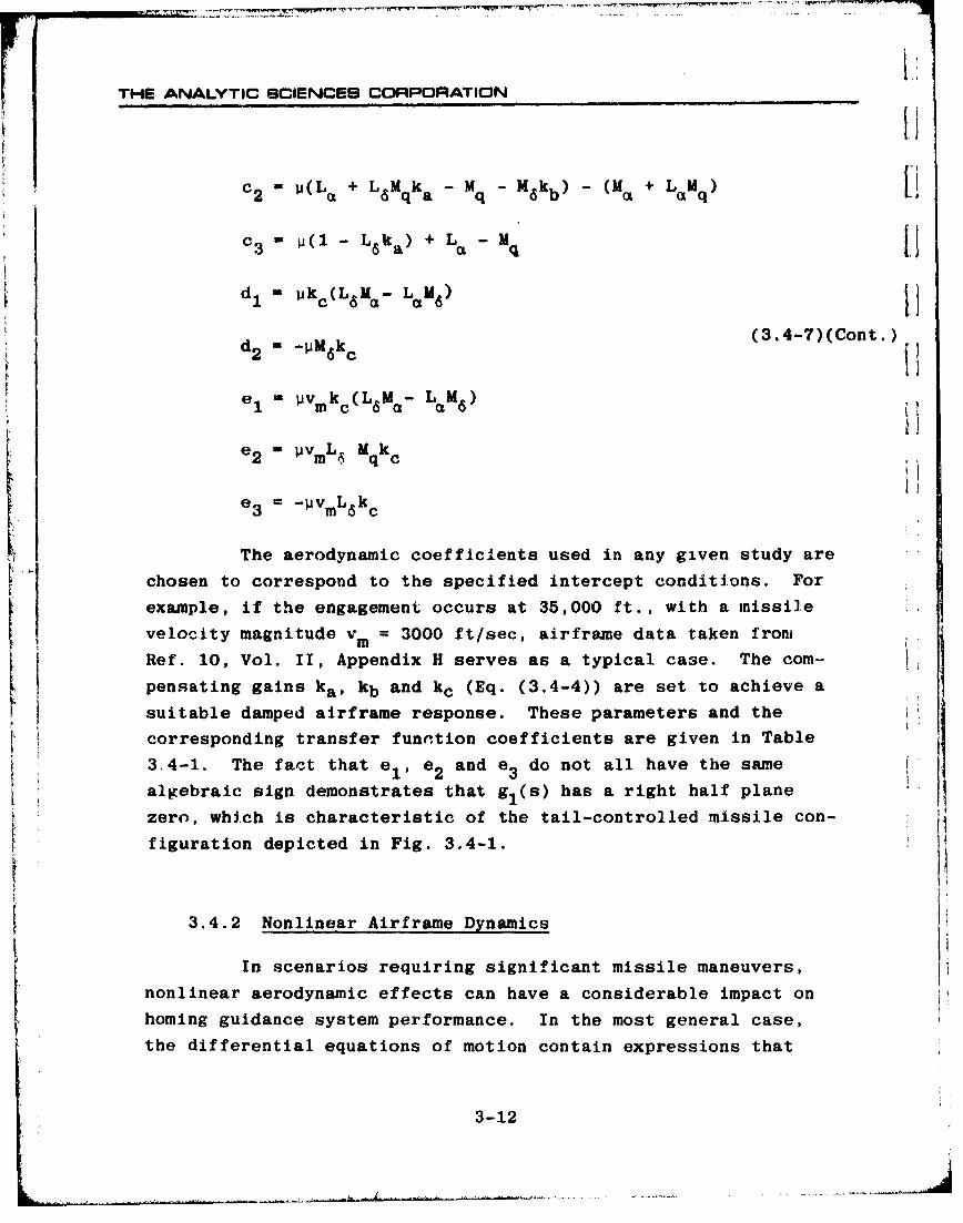
Il =J 1(k a+kb) (L 6 Ma LaM 6 )-M.- LgM q] (3.4-7)
' •3-11
THE ANALYTIC SCIENCES CORPORATION
-(L M kb) - (Ma + LM) [q
c 3 w- (1L 6 k a )+ L ~Mq [d, - Ikc(L 6Sa- L M6 )
d (3.4-7)(Cont.)
el - VImk c(L 6 M - LaM 6 )
I)
e2 - pVmLA Mqkc
e = -jv L k
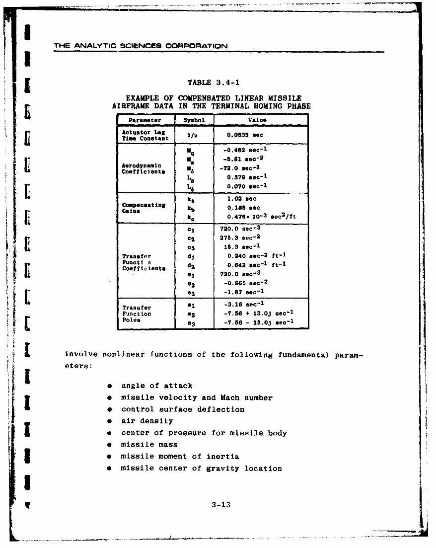
The aerodynamic coefficients used in any given study are
chosen to correspond to the specified intercept conditions. For
example, if the engagement occurs at 35,000 ft., with a missile
velocity magnitude vm = 3000 ft/sec, airframe data taken from
Ref. 10, Vol. II, Appendix H serves as a typical case. The com-
pensating gains ka, kb and kc (Eq. (3.4-4)) are set to achieve a
suitable damped airframe response. These parameters and the
corresponding transfer funntion coefficients are given in Table
3.4-1. The fact that el, e 2 and e3 do not all have the same
algebraic sign demonstrates that gl(s) has a right half plane
zero, which is characteristic of the tail-controlled missile con-
figuration depicted in Fig. 3.4-1.
3.4.2 Nonlinear Airframe Dynamics
In scenarios requiring significant missile maneuvers,
nonlinear aerodynamic effects can have a considerable impact on
homing guidance system performance. In the most general case,
the differential equations of motion contain expressions that
3-12
THE ANALYTIC SCIENCES CORPORATION
5 TABLE 3.4-1
EXAMPLE OF COMPENSATED LINEAR MISSILEAIRFRAME DATA IN THE TERMINAL HOMING PHASE
Parameter Symbol Value
Actuator Lag i/ 0.0533 sec
Time Consta~nt
Mq -0.462 nec-1
Aerdyi M -5.81 sec-2Aerodynamioci -72,0 sec-2Coefficients
La 0.379 sec-1SL6 0.070 sec 1
ka 1.02 secCompensating kb 0.188 sacGains k 0.476x I0-3 sec2 /ft
ci 720.0 sec-3
C2 275.3 sec- 2
c3 18.3 sec- 1
Transfer dl 0.240 sec- 2 ft-1Functi a d2 0.642 see-' ft-1Coefficients 01 0.4 sec- t
20 -I70.06 gec"3
e3 -1.87 sec-1
Transfer a1 -3.16 sec- 1
Function 82 -7.56 + 13.0J sec"1
Poles3 -7.56 - 13.0J sec-1
I [involve nonlinear functions of the following fundamental param-eters:
* angle of attack* missile velocity and Mach number
control surface deflection• air density
center of pressure for missile body* missile mass3 * missile moment of inertiae missile center of gravity location
S3-13
THE ANALYTIC SCENCES CORPORATION
The development of a nonlinear aerodynamic model requires
a somewhat greater degree of specificity than that needed for the
general discussion of the linear case given above. For this rea-
son, we confine our attention to a missile modeling problem that His similar to that detailed in Ref. 3. The resulting nonlinear
model is typical of tail-controlled cruciform missile airframe
dynamics under tha conditions noted below.
During the terminal intercept phase, the missile is as- Hsumed to be in a gli:, n,.•tt' of operation, corresponding to a thrust
force of zero. Consey,.i•'•y, missile mass, mome:_t of inertia, and
center of gravity ,4re constant and need not be considered as vari-
ables in the airframe equations. The assumption that the inter-
cept plane is nearly horizontal in the last few seconds of an
engagement implies that the free stream air density, p., and the
speed of sound, vs, are constants. The latter condition allows us
to use missile velocity, Vm, and Mach number, vm/vs, interchange-
ably. The variables of the required nonlinear airframe equations A
of motion are then defined in Fig. 3.4-1.Li
The lateral component of missile acceleration, aV, results
from the lateral aerodynamic force which is assumed to be separable [
into contributions Ftaot and Ffd due to nonzero angle of attack i
and fin deflection, respectively. Similarly, the axial component
of missile acceleration, aa, is due to the axial force contributions
Faaot and Fafd due to a and 6. The positive sense of a, is chosen
to correspond to the sense of the lateral forces produced by posi-tive a and 6, respectively, and the positive sense of aa corres-ponds to positive drag. Letting m denote the mass of the missile
during the terminal intercept phase, the acceleration components
a• and aa can be expressed in terms of these force components as
at (F aot Fa• Faot fd)/
(3.4-8)
a a (Faaot a
at3fd -1Li1

THE ANALYTIC SCIENCE3 CORPORATION
It is then a simple derivation (Ref. 3) to show that
&IE + (vF~ao + Ffd sin a - (Flaot + F
(3.4-9)
The differential equation for body angular rate, 6 M) is
obtained from the summation of the moments acting about the body
principal axis. The body lateral force Ftaot acting on the air-
I frame at the body center of pressure, and the control surface lateral
force FXfd acting at the center of pressure for the tail are primary
contributions to the moment equation. Other aerodynamic moments
l I: may also be significant; for example, rotation of the missile body
produces a moment m that is sometimes not negligible. Letting Ibq q
! L denote the missile moment of inertia about the body axis and letting
d a and d6 denote the respective moment arms through which the forces
FXaot and FXfd act, the expression for the missile body angularacceleiationi is
i Lk 6m = - (at + F, d6+ mq (3.4-10)
The rate of change of the magnitude of the velocity vec-
tor can be obtained from the projection of the body acceleration
components onto the velocity vector. This procedure, followed by
the substitution of Eq. (3.4-8), yields
1 mo aaot afd )cosa aot fd
(3.4-11)
The above lateral and axial forces are in themselves a
source of nonlinearity. For example, they are proportional to
I the dynamic pressure, q., given by
1 13-15
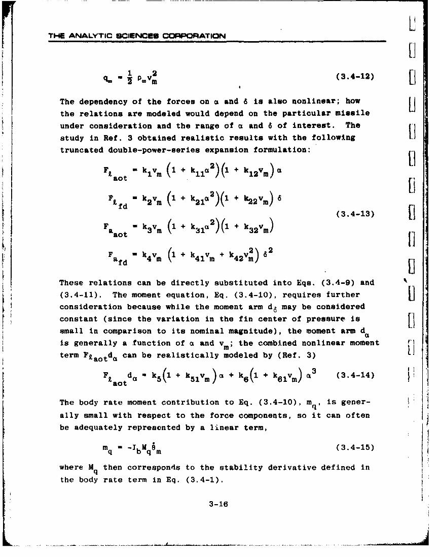
THE ANALYTIC SCIENCES CORPORATION
1 2 (.-2q= PDV m (34-2
The dependency of the forces on a and 6 is also nonlinear; how Uthe relations are modeled would depend on the particular missile
under consideration and the range of a and 6 of interest. The
study in Ref. 3 obtained realistic results with the following
truncated double-power-series expansion formulation: ,
Ft at k k1vM (1 + k 11ca2)(1 + k12 VM)o [aaot [
I fd w 2vm ( 2 X k2)( vm)
Fa aot k3 (1 + k3 2)@ I k 32 v) (3.4-13)
2)[2F a k 4 1Vm + k 4 2 Vv)2 6uaid
These relations can be directly substituted into Eqs. (3.4-9) and
(3.4-11). The moment equation, Eq. (3.4-10), requires further Uconsideration because while the moment arm da may be considered
constant (since the variation in the fin center of pressure is
small in comparison to its nominal magnitude), the moment arm d
is generally a function of a and v m; the combined nonlinear moment
term Ftaotda can be realistically modeled by (Ref. 3)
Faotda k5(1 + k5 1 vm )a + k(1 + kv) (3.4-14)
The body rate moment contribution to Eq. (3.4-10), mq, is gener-
ally small with respect to the force components, so it can often
be adequately represented by a linear term,
mq - bqm (3.4-15)
where Mq then corresponds to the stability derivative defined in
the body rate term in Eq. (3.4-1).
3-16

THE ANALYTIC SCIENCES CORPORATION
A further simplification of the basic aerodynamic dif-
ferential equations, Eqs. (3.4-9) to (3.4-11), can be achieved
by making suitable small-angle approximations to the trigonometric
functions involved; this entails truncating the series
sin ai a- + 13 + ...
~~ lb cos a a~ci +..
at a point consistant with the range of a and the accuracy of thenonlinear representation of the normal and longitudinal forces,
SrEq. (3.4-13). The basic equations then contain only terms of the
form ak 6 pvm for which quasi-linear gains may be derived directlymusing Cases 1 to 3 of Section 4.3.2; many results of this form
Sare given in Appendix A.
To relate the nonlinear model to the linear case givenin Eq. (3.4-1), we observe that the linear terms of Eqs. (3.4-9)
to (3.4-14) with vm taken to be constant are equivalent if
SL [ik(1 + k 1 2 v•)-k 3 (1 + k 3 2 V)]
kL• 2 • (1 + k22Vm)
SI ~i)(3.4-16)
Ma - (1 + k1v)I5 Mb
~k2K I M - (1 + kv) d
The nonlinear model of the autopilot-airframe module iscompleted by deriving a formulation of the control fin actuator
3IS• ~3-17"

EANALYTIC SCIENCES Ci-PORATION
dynamics and compensation. A simple linear model ror this func-tion is given in Eqs. (3.4-3) and (3.4-4), viz.
- -�j6 + Pu(t) H(3.4-17)
U k a k aa- kb
with typical parameter values given in Table 3.4-1. If there aresignificant nonlinear effef ts to be modeled, such as actuatorsaturation, hysteresis, nonlinear friction or the like, then itmay be necessary to develop a much more detailed representation.An example of a complete autopilot/airframe model in which con-
trol fin actuator saturation is included is depicted in Fig.3.4-4.
3.5 THE GUIDANCE SUBSYSTEM MODEL
The operation of the guidance module may be separated
into two cascaded functions: filtering of the signals obtainedfrom the seeker in order to reduce the effect of measurement noise,and control of the missile lateral acceleration on the basis ofthe filtered measurements. There are a number of filtering andcontrol schemes that can be used in tactical missile design, asreported in Refs. 9 and 10. The systems that result may be di-vided into analog guidance modules in which the missile accelera-tion command is obtained by standard analog techniques which maybe modeled using continuous-time dynamic equations, and digitalguidauce modules in which filtering is accomplished using discrete-time data processing techniques, including sophisticated algorithmsbased on modern estimation theory (extended Kalman filters), andthe control function may be based on optimal control theory. Inthis section, we treat the classical proportional guidance law asan example of the first category, and discuss several alternativedigital guidance systeris based on the use of a Kalman filter.
3-18
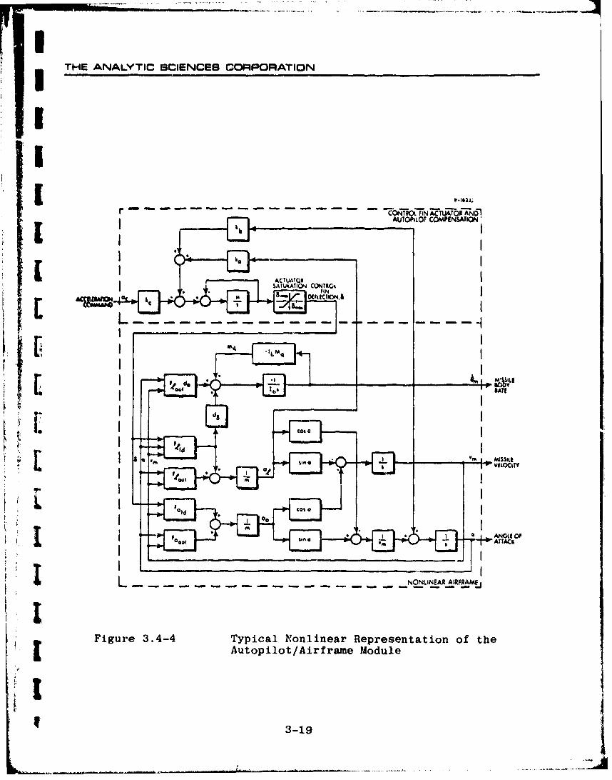
THE ANALYTIC SCIENCES CORPORATION
r - - - - -FIN -AC, ,=ORA--
I ~AUTOPILOT COMPEN0SATAONII
I Ih ,;
I -.
$oAIUKAflON W O
9-L - - - - -. .
d. myI
iii
3-1ATE
VIUXI, TY
fl col a
L -. . . - --.. . .- - - - - NONLINEAR AIRFRAMEj,
S[Figure 3.4-4 Typical Nonlinear Representation of the• Autopilot/Airframe Module
Jr 3-19
THE ANALYTIC SCIENCES CO•FPORATION
3.5.1 Proportional Guidance
The guidance signal available from the seeker (n in
Fig. 3.1-1) is typically a variable proportional to LOS angle irate, 6, corrupted by measurement noise. This signal is passed
through a single-stage low-pass noise filter, the output of which Iis thus a filtered estimate of LOS angle rate, 8 6. The pro-
portional guidance law is then implemented, which calls for the Icomponent of missile lateral acceleration that is normal to the
line-of-sight (LOS) to be proportional to the closing velocitytimes the estimated LOS angle rate.
This guidance law is based on the concept of the missile- Itarget co1V'sion triangle. In a simplified scenario in which the
target is following a straight line trajectory, with constant 1aspect angle ea and velocity vector magnitude vt, the most effi-
cient intercept path for the missile (assuming its velocity, vml
is also constant) is a straight line specified by a constant lead
angle O•, chosen such that the cross-range components of the mis-
sile and target velocity vectors are equal: avm sin = v sin 0 (3.5-1)
If the missile lead angle is not equal to 0k, then there is a
nonzero heading error, 0 HE, given by
eri - - 0£ (3.6-2) i
We observe that flight along the collision triangle (along the
vector v*, Fig. 3.5-1) results in a nonrotating LOS, i.e.,b = 0.
Thus 6 can be considered the error signal for this guidance
strategy.
For the purpose at hand, we assume that the missile
acceleration vector 4n is normal to the velocity vector (6va is
3-20

ITHE ANALYTIC SCIENCES CORPORATION
Sy fl.t47o
"IDEAL MEAN MEAN TARGETCOLLISIONMENTRTCOURSE TRAJECTORY
MISSILE TARGETVELOCITY. ym VELOCITY, Vt
[ INITIAL LINE-OF-SIGHT
Figure 3.5-1 Deviation from the CollisionCourse Triangle
* 90 degrees in Fig. 3.2-1); thus we desire to generate an accelera-
tion command to cause am to satisfy
am cos( -8) n'v.4 (3.5-3)
where the parameter n' is called the navigation ratio. The clos-
ing velocity i obtained by projecting th( -issile and target
velocity vectors onto the instantaneous line of sight; as shownS~in Fig. 3.2-1,
v= V cos (6 - 0 ) + vt cos (6 +a0) (3.5-4),*-r Z= vm a,+e 35
In order to achieve a response that obeys Eq. (3.5-3), the ideal
acceleration command a' should be chosen to satisfy
nyc0
ac C (3.5-5)
where the incorporation of the factor 1/cos (0 -) as dictated
by Eq. (3.5-3) is known as secant compensation.
i
THE ANALYTIC SCIENCES CORPORATION
rI
In mechanizing the guidance law, the value of the closing
velocity is never kiown exactly. If a radar homing seeker is used,
then a reasonable estimate of v can be obtained by doppler mea-
surements or by differencing range measurements. An infrared seek-
er system generally does not yield a good estimate of range, in
which case vc may be taken to be a prespecified constant. Any
uncertainty in the closing velocity is modeled by introducing a
variable e into Eq. (3.5-5) which represents either a band limitedvnoise, obtained by a single-stage low-pass filter with white noise
input, or a bias, denoted simply evb. Thus, for example,
"F + vt cos(ea + 0) + evlac n cos(e - e (3.5-6)
provides the final acceleration command used in Ref. 4, where e
is modeled by one of the differential equations
Random Uncertainty: ev = -•W4 ev + w,, E Lev(O)] = 0 3(3.5-7)
Bias Uncertainty: e6 = 0, e v(0) evb
and w4 is white noise with spectral density q 4 " With this model
we can study either the effect of the noisy estimation of vc or
of a constant error in the assumed value of v C"
Finally, the guidance law must account for an important
nonlinear constraint on missile operation -- acceleration command
limiting. The act. U1 acceleration command ac that determines the
input to the fin deflection ictuator in Figs. 3.4-2 or 3.4-4 must
not exceed the structural capacity of the airframe and must not be
so large as to cause the missile to stall. Thus the above idealized
acceleration command a' must be limited in order to prevent exces-
sive lateral acceleration command levels or angle of attack; the
limiting procedure is represented by the saturation nonlinearity
3-22

THE ANALYTIC SCIENCES CORPORATION
ac l'ac • c ' c1- amaxa' m (3.5-8)
ama sign (a,), Jac[ >max, > armax
The guidance law features described above are incorporated,U in the system model illustrated in block diagram form in Fig.3.5-2.
1. to115,9 b
CLOSING VELOCITYERROR MODEL
W 2 1 V * V + " t C 0 5 ( 8 0 + 8 )
ESTIMATE rs
NOISE FILTER CLOSING VELOCITY WITH SECANT ACCELERATIONCOMPENSATION AND UNCERTAINTY COMMANDS
1 [Figure 3.5-2 Proportional Guidance Law Modeli Fi3.5.2 Modern Digital Guidance Systems
Recently-proposed high-accuracy guidance systems for tac-
tical missiles have been designed using digital data processing andlb optima] estimation and control theory. The resulting combination_• of Kalman filter and optimal control law that comprises the digital
guidance module is generally based on a linear system representa-
tion ("filter model") that is significantly less detailed than thez simulation model ("truth model") which strives to represent allimportant dynamic effects. Quantities that can be assumed to beavailable to the filter without measurement noise are treated asdeterministic inputs to the filter and thus need not be consideredin the model (Ref. 11). To obtain a filter model that is linear in
r3-23
THE ANALYTIC SCIENCES CORPORATION
the variables of interest, all nonlivearities that occur in the {ftruth model are replaced by constant or time-varying gains derived
by small-signal or Taylor series linearization.
Kalman Filter Model - A basic 3-state Kalman filter can
be designed for the missile-target intercept problem using themodel depicted in Fig. 3.5-3. It is assumed that noisy measure-ments of LOS angle, 0, are available to the filter in conjunction jjwith noise-free measurements of missile lateral acceleration andmissile-target range. The range information is required in the
filtering procedure because the LOS angle is assumed to be relatedto the cross-range separation, y, by the time-varying gain 1/r, andthe measurement noise sequence vk (Fig. 3.5-3) is range dependent,as detailed below; the Kalman filter algorithm makes use of know-ledge of these dependencies in generating estimated values of the Hfilter state variables, denoted f
In state-space formulation, the filter model is given by Lithe vector differential equation
;f = Ffxf(t) + Efw5 (t) + dfam(t) (3.5-9)
where
I 0 1 1 0- 0
xf Ff 0,0dff 0-at- 0 0 J
(3.5-10)
and w5 is the white noise process which is the input to the tar-
get acceleration model (Section 3.3). The white noise process w5is specified by its mean and spectral density,
E [w5 (t)] = (
E[w5 (t) w5 (T)] 6(t-)
3-24
• .t . . . . . . . . ..... • .. . . . . . . . . . . . . . . . . . ... . . . . .. . . . . . . • . , - ':

IiTHE; ANALYTIC SCIENCE3 CORPORATION
1 MEASUREMENT VkNOISE SEQUENCE
IiTARGET LATERAL CROSS-RANGE LOS
ACCELERATON,at SEPARATION, y ANGLE.,6
iWHITENOISE T
'INPUli MISSILE LATERALACCELERATION, am rnT
MISSILE OL INTEIAR y KALMAN
DYNAMICS GUIDANCE FILTER
LAW
ACCELERATION ESTIMATED STATECOMMAND, ac VARIABLES, Of
Figure 3.5-3 Missile-£arget Intercept Model for the|L Derivation of the Digital Guidance Module
SI.The vector xf is initially specified by the mean vector
mf(O) and covariance matrix Pf(O); observe that these may or mayBf
not be directly related to the statistical initial conditions on
lb the truth model state vector, since the filter model variables
are not necessarily a subset of these states. In the kinematics
• Tsubsystem model, for example, k Is generally not a state variable;
rather the time derivative of the state y is a nonlinear function
of the states 0 X (missile lead angle) and 6a (target aspect angle)
as given in Eq. (3.2-2),
=-v sin G + v sin Oam +vt a
T 3-21r
..............................[----~----.~.-...--

THE ANALYTIC SCIENCES CORPORATION
in which case
mf (0) - E [k(O)] - -vm E [sin 0 (0)] + vtE [sin ea(0)]
-ipex -*pea
=-vme sin m + ve asin m (3.5-12) 11m t SS~a
where me, and PO are the mean and variance of 6,, respectively,mea and pea refer to the same statistics of ea' and use has been
made of the result
E [sin x] f e sin m x
(Ref. 3; see also Eq. (4.3-10)). The variance of k(0) can becalculated from the statistics of a (0) and 0 (0) in a similar
a2manner. It is also possible to choose mf(O) and Pf(O) to beinconsistent with the truth model state initial statistics, to
determine the performance of the filter when its initialization Liis in error.
The model shown in Fig. 3.5-3 can be derived directly fromthe results given in other sections of this chapter under the sim- !plifying assumptions that
e Missile and target acceleration vectors(Fig. 3.2-1) are normal to the respectivevelocity vectors (velocity vector magni-tudes are constant).
9 Kinematic nonlinearities (Fig. 3.2-2) arenegligible.
* The target maneuver is represented by aband-limited gaussian process (Fig. 3.3-1).
9 Seeker dynamics (Section 3.6) are negligible.
3-26
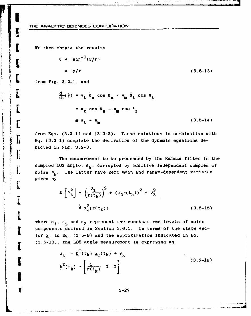
II
THE ANALYTIC SCIENCES COR:PORFATION
,[ We then obtain the results-1
0 s sin (y/rA
a y/r (3.5-13)
Sfrom Fig. 3.2-1, and
S1 () " Vt a Cos ea -vm 01 Cos C i
M a cos a - a cos0t a m Z
a a t - am (3.5-14)
from Eqs. (3.2-1) and (3.2-2). These relations in combination with
Eq. (3.3-1) complete the derivation of the dynamic equations de-
picted in Fig. 3.5-3.
The measurement to be processed by the Kalman filter is the
sampled LOS angle, 0 k, corrupted by additive independent samples of
SI noise vk. The latter have zero mean and range-dependent variance
given by
[v2] (t) + (o 2 r(tk)) + a2k r(tk)2 k3
a v(2r(tk)) (3.5-15)i-"
where al' 02 and o3 represent the constant rms levels of noise
components defined in Section 3.6.1. In terms of the state vec-
tor xf in Eq. (3.5-9) and the approximation indicated in Eq.
(3.5-13), the LOS angle measurement is expressed as
Zk = hT(tk) )Cf(tk) + vk
k __ 00) (3.5-16)
ShT(tk)=[ir~tk) o]
f 3-27

THE ANALYTIC SCIENCES CORPORATION
rho discrete Kalman filter providos an estimate, xr., of
the reduced-order state vector xf utilizing mechanization equa-
tions (Ref. 11) of the form
xf(t) - Ffxf(t) + dfam(t), tk_ < t < tk (3.5-17)
^ + T
xf(tk) - xf(tk) + k (_k-h(tk)xf), tk < < k t (3.5-18)
where _xf(tk) denotes the solution to Eq. (3.5-17) just before a
measurement is processed, and xf(tk) represents the state vector
estimate after the measurement and update take place*. The gain
vector kk is obtained recursively from the matrix covariance equa-
tion associated with the Kalman filter; the sequence of operationsis given by: (i) propagation of the filter covariance matrix
according to
+ •TP k - 0 P k-1 It +(3.5-19)
where P is the value of the filter covariance matrix after the
previous update, $, given by
SA exp (FfTs) (3.5-20)
is the transition matrix expressed in the usual matrix exponential
form, T. = tk- tk1 is the time interval between samples, and
T TS~s Ff(Ts-t)gfKT eFT(rs-t)
0q5 e e dt (3.5-21)
Refer to the footnote on page 1-15.
3-28

THE ANALYTIC SCIENCES CORPORATION
is the noise covariance matrix; (ii) calculation of the Kalman
gain vector,
hk -Pkhk 4-k+o~rt)) (3.5-22)
"(iii) updating the filter covariance matrix (to represent the
effect of updating the state vector estimate)
P P T (2 )kT (3.5-23)
It is likely that tk.e range-dependent gain vector in this example
can be precomputed and stored as a function of range if range in-
formation is available in the guidance module. Otherwise, the
L implementation of Eqs. (3.5-22) and (3.5-23) would be responsible
! [A for most of the digital computational capability required by this
guidance system.
Equations (3.5-17) to (3.5-23) are a set of typical Kal-
man filter mechanization equations based on a simplified design
4, model. The filter state estimates y, y and at provide the basis
for the missile guidance law which generates the commanded missile
lateral acceleration, denoted ac in Fig. 3.4-2. An optimal control
approach to developing a guidance law is described below.
4.- Control Law Model - An optimal control policy is derived
by selecting the commanded acceleration time history to minimize
A an appropriate performance index. An index that is found useful
for the missile guidance problem is the so-called quadratic index,
I E Y2(tf) + Ytf%( )2 dt (3.5-24)
which effectively minimizes the expected value of the square of
the miss distance while imposing a penalty on the control level.
The quantities y(tf) and y are the terminal miss distance at
L 3-29
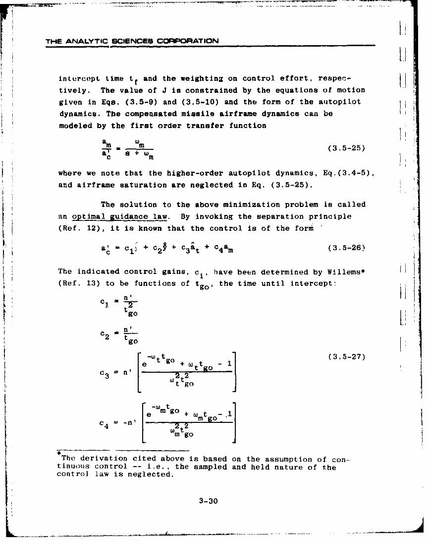
THE ANALYTIC SCIENCES CORPORATION
inturcept time tf and the weighting on control effort, respec-g n(a .nf fttively. The value of J is constrained by the equations of motion
i given in Eqs. (3.5-9) and (3.5-10) and the form of the autopilot
dynamics. The compensated missile airframe dynamics can be
modeled by the first order transfer function
am WI (3.5-25)ac .1 + wjm
where we note that the higher-order autopilot dynamics, Eq.(3.4-5),
and airframe saturation are neglected in Eq. (3.5-25).
The solution to the above minimization problem is called
an optimal guidance law. By invoking the separation principle
(Ref. 12), it is known that the control is of the form
a. c= " + + a + c 4 am (3.5-26)
a' +1 c2 ~ C3 t (3.-26
The indicated control gains, ci, have been determined by Willems*
(Ref. 13) to be functions of tgo, the time until intercept:
=90
t IgC n
tgo
_[-Wte •ttgo _ (3.5-27)St go+-
W [t go
C4 f-nf' 2 2]
•m go
The derivation cited above is based on the assumption of con-
tinuous control -- i.e., the sampled and held nature of thecontrol law is neglected.
3-30

THE ANALYTIC SCIENCES CORPORATIONIThv Iimv--to-intr(-rcpl, tg. and optimal nnvigntlon ratio. n', aregiven by go
K tgo - tf - t •clt.O -t (3.5-28)
[where vc is the closing velocity, Eq. (3.5-4), and
iI3t 2 Ft 1-e (-e m t g°o
n' = -o . m Igot
T 31 - -3 tm O+ 2e-(mtgo)/+ t 2 O ( 3go 5-29)
'The expression for n' is considerably simplified if the compen-
sated airframe dynamics are neglected entirely; from Eq. (3.5-25)0
Sm=a' if we permit wm to approach infinity, in which case
3n' (3.5-30)
m go
If there is no constraint on acceleration, y is equal to zero andK 'the resulting navigation ratio from Eq. (3.5-30) is constant.
Finally, in implementing the control given in Eq. (3.5-26),
it is often advantageous to use an alternative formulation for tgo;
t - r (3.5-31)Igo vc r
Using the instantaneous value of range divided by closing velocity
is equivalent to Eq. (3.5-28) when range is nearly deterministic.
This expression is conveniently evaluated in the digital guidance
module using a discrete approximation to the derivative; at each
sampling instant
gok r (3.5-32)
3-31
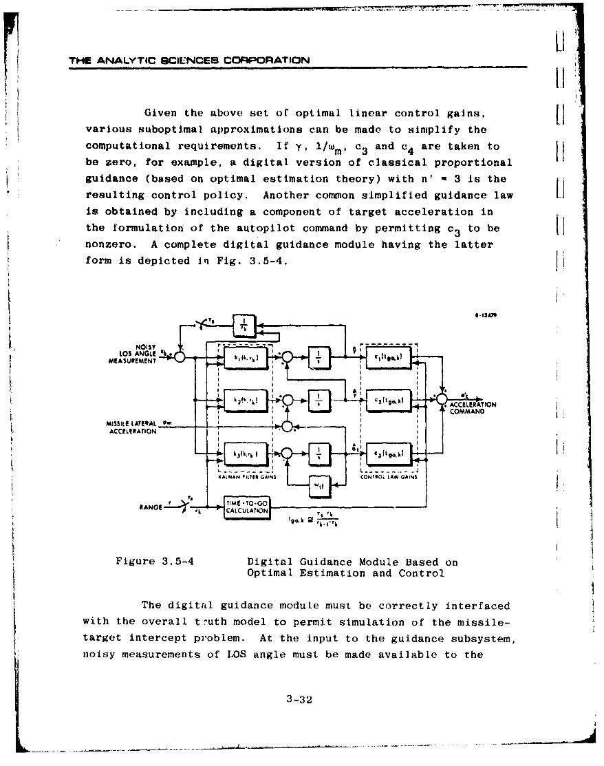
LITHE ANALYTIC SCILNCES COR:PORATION
Given the above set of optimal linear control gains, Hvarious suboptimal approximations can be made to simplify the
computational requirements. If y, l/w m, c3 and c 4 are taken to Hbe zero, for example, a digital version of classical proportional
guidance (based on optimal estimation theory) with n' - 3 is the
resulting control policy. Another common simplified guidance law
is obtained by including a component of target acceleration in
the formulation of the autopilot command by permitting c 3 to be 1)nonzero. A complete digital guidance module having the latter
form is depicted In Fig. 3.5-4.
NOISY
LO S ANG LE 't rk ) (t, 'tl
MEASUREMENT
A R ACCELETATION
ACLRATINGE.'TM-O
L!
The digital guidance module must be correctly interfaced
with the overall t-uth model to permit simulation of the missile-
target intercept problem. At the input to the guidance subsystem,
noisy measurements of LOS angle must be made available to the
3-32

ITHE ANALYTIC SCIENCES CORPORATION
1 ~~K.11111:11% rilit'j.. Ho IM .-; th i rwgl~l i, ,ol tnnod i,• potie. M v l ol v l, r -
mined by the specific seeker design and hardware considerations.
A variable which is often readily available as the seeker output
is n, shown in Fig. 3.6-9, which is an approximate noisy measureof line-of-sight angular rate; to be more precise, it is demon-
I • strated in Saction 3.6.3 that n is related to the LOS angle 0 by
dynamics that can be approximately represented in transfer func-
[ tion form as
s " +(3.5-33)
where Td represents the dominant time constant of the overall
seeker track loop. Thus a direct method for obtaining the re--- quired filter input signal from the seeker output n is to inLer-
pose a prefilter of the form
hf(S) - Td + 1 (3.5-34)
* , to provide effective compensation for the dominant pole in the
seeker dynamic model.
Another factor in implementing the guidance law is that
the ideal acceleration command ac given in Eq. (3.5-26) is based
on the assumption that missile acceleration is normal to the LOS.As in the previous section (cf. Eq. (3.5-3)), the fact that am is
I actually nearly normal to the velocity vector requires secant com-pensation (division by cos (e -e)) to guarantee that the accel-
eration command leads to a suitable acceleration component normalto the LOS.
I The guidance module design is completed by incorporatingan ideal limiter to prevent excessive acceleration command levels.
An overview of a typical digital guidance module based on theforegoing discussion is shown in Fig. 3.5-5.
3* 3-33

'THE ANALYTIC SCIENCES CORPORATION
IiRANGE,-
A% ISILE LATERALACCELERATION, om
LOS RAT LOS ANGLE DELAY
ESTIMATE MEA.UREMIENT OPTIMAL COMPEN&ATED ACAL
)PLAN T IM4 VAL a
PR[~tE ETI'~FILTER CONTROL ACCo LEg ATION CO(81.AN8S
Figure 3.5-5 Complete Digital Guidance Module Structure
3.6 TH1E SEEKER SUBSYSTEM MODEL
There are several effects inherent to the seeker which can
have a marked influence on overall missile performance. These in-
clude o I.4t
* Boresight error distortion sources
NoiseAberrationReceiver and signal processing characteristics
0 Disturbance torque sources
Seeker mass imbalance 'I
Seeker gimbal frictionSpring restoring forces on the seeker head
:3.6.1 Boresight Error Distortion
A fundamental variable in the seeker subsystem is the
true boresight errer, -true defined by the angle between the
antenna centerline and the instantaneous line-of-sight (LOS) to
the target; referring to Fig. 3.6-1,
tre = - h - = (3.6-1)
3-34
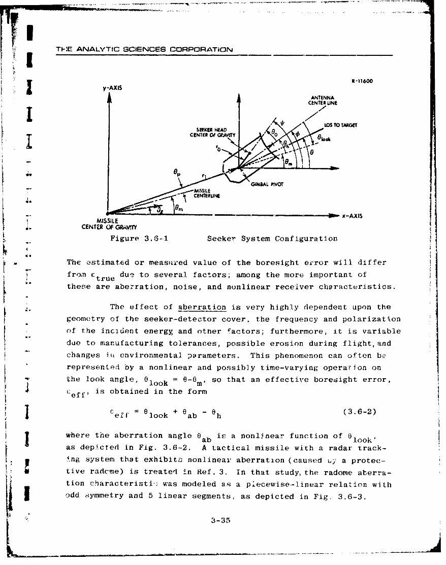
F.TE ANALYTIC SCIENCES CORPORATION
R-11600y-AXIS
ANTENNACENTER UNE
SEEKER H'EAD O OTRE
CENTER Of GPAVITY 08
'°> AXIOloo
hGIM&AL InOT
.- # ,rt=0- x-AXIS
MISSILEI,, CENTER OF GRA•VYFigure 3.6-1 Seeker System Configuration
The estimated or measur'ed value of the boresight er'ror will differ
from ctrue due to several factors; among the more important of
L these are aberration, noise, and nonlinear receiver characteristics.
The effect of aberration is very highly dependent upon the
geometry of the seeker-detector cover, the frequency and polarization
of the inc-dent energy and otner factors; furthermore, it is variable
due to manufacturing tolerances, possible erosion during flight, and
changes iu environmental parameters. This phenomenon can often be
represented by a nonlinear and possibly time-varying operation on
Sthe look angle, 0look = 6-0m, so that an effective boresight error,
i'eff' is obtained in the form
J eff Elook +ab - Eh (3.6-2)
I where the aberration angle e ab is a nonlinear function of 0 look'as depicted in Fig. 3.6-2. A tactical missile with a radar track-
:'ng system that exhibits nonlinear aberration (caused 6y a protec-
K • tive radcme) is treated in Ref. 3. in that study, the radome aberra-
tion characteristi,: was modeled as a plecewise-linear relation with
odd symmetry and 5 linear segments, as depicted in Fig. 3.6-3.
1k ,; 3-35
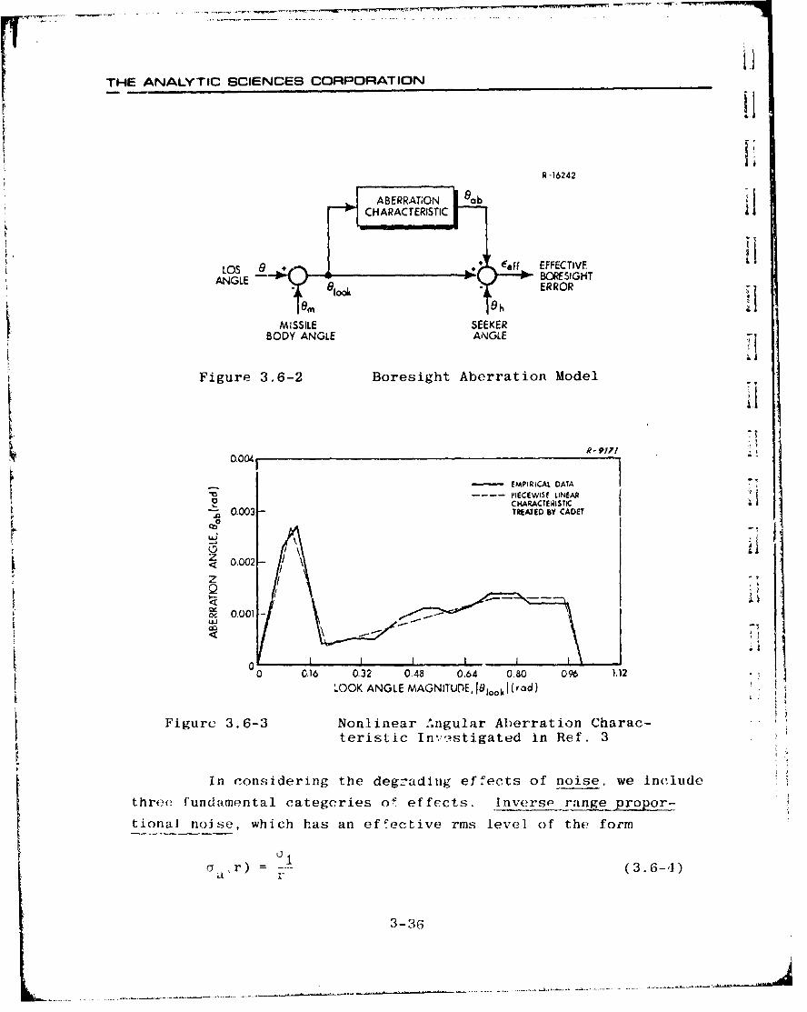
THE ANALYTIC SCIENCES CORPORATION
R -16242
LOS 8 + eaff EFFECTIVE.ANGLE OEIH
MISSILE SEEKERBODY ANGLE ANGLE
Figure 3.6-2 Boresight Aberration Model
-EMPIRICAL DATA
-_ - ICWIFLNA
THE ANALYTIC SCIENCES CORPORATION
w t re 0 1 is a constan t, is rcpt t.ese t.; t i" % :- .' oist- soiji-ev (hat
increases in effect as range approaches zero. Target angular scin-
[ tillation (caused by the apparent motion of the target due to the
change in position of the target controid of radiation) is a phenom-I enon of this sort. This effect can be modeled as a wide-band noiseL state,* xl, with constant rms level, a1 , multiplied by a gain 1/r.
Range proportional noise includes any noise source that yields an ef-
fective noise level that decreases as the missile approaches the tar-
get, i.e., as range approaches zero. This type of random disturbance may
, be represented by an equivalent noise with an rms level of the form
ab(r) = 2: (3.6-5)
which in turn can be modeled by a wide-baad nuise state x 2 with a
constant rms level of 02 passing through a gain r. Noise sources
that exhibit this property are the distant stand-off jammer and[receiver noise (generally due to thermal effects). Range independent
noise represents noise sources that have a constant effect on theT'
signal-to-noise ratio; target amplitude scintillation (due to time-
varying effective target cross section, for example) and seeker
r servo noise are typical examples of noise sources that can be3 2modeled by a noise state x 3 of constant vai_"nce a3. The complete
noise model is shown in Fig. 3.6-4 where wl, w2 , and w3 are gaus-
sian white noise processes.
All three types of noise described above have been treated
in previous studies (Refs. 2 to 4), in two forms. The most ele-
T mentary implementations of this model may be taken to be linear
I time-varying; i.e., r(t) is assumed to be deterministic in the
noise model. In a more recent treatment, Ref. 4, the nonlinear
I relation indicated in Fig. 3.6-4 is rigorously implemented by
Where no conventional state variable nomenclatiure is suggested,arbitrary state numbers are assigned for convenient reference.
3-37
i

LiTHE ANALYTIC SCIENCES CORPORATION
R-116CL;
1Ii
WHITENOISE" w~ sEETOTANOS 2NOISE
Figure 3.6-4 Seeker Noise Model
"n = + x 2 /x2+y2 + x3 (3.6-6)x .
where xl, x 2 and x3 are the wide-band noise states mentioned above
and x and y are the cartesian components of missile-target separa-.
tion, respectively (see Fig. 3.2-1). The linear time-varying
formulation may be adequate in situations where range has a negli- Hgible random component (as is sometimes the case for the head-on
intercept where the mean missile lead angle and mean target aspect
angle are both zero), but Eq. (3.6-6) is generally significantly
more accurate when the range is appreciably nondeterministic. UThe receiver characteristic is a potentially complicated
effect, highly dependent upon the specific antenna design, type of
detector, and signal processing scheme. In order to avoid a very
specialized discussion based on a particular tactical missile, we
confine our attention to one basic phenomenon: the attenuation of
the received signal which occurs when the effective boresight error,
Ceff, becomes large, i.e., when c approaches cmax in Fig.3.6-5a.
The detector alone will have an output which is very nearly pro-
portional to its input for siaall values; however, as the effective
boresight error magnitude approaches cmax' we n.te i.n Fig. 3.6-5b
3-38

THE ANALYTIC SCIENCES CORPORATION
[ ,.-1160317 ANTENNAL ~aNTEUJNE
S~L IN E O f S IG H T
0 Off -%*4`MAIN
•ANEA..... •------ • _.
PATTERN
i Ia
ANThENA POSSIBLESIDE LOBE
ii "-
(a) Antenna Sam Pattern
ddet dueI; u
(b) Antenna-Detector Characteristic (c) Signal Processing Nonlinearity
L Figure 3.6-5 Receiver Boresight Error Distortion Effects
that the signal strength decreases to a null. If the antenna pattern
has appreciable sidelobe sensitivity, there may also be some response
for values of c greater than c The upper limit on the bore-•.fo v lu s f eff g e t r h a m ax *
sight error, E, such that the detector characteristic is nearly
£linear for i 'effI less than £,is quite variable, depending on the
type of target tracking system under consideration. For monopulse
radar or infrared detectors, j could be as small as a fraction of a
degree (Ref. 14).
K £The undesirable detector null and possible spurious side-
lobe response can be circumvented in the signal processing scheme.
3-39---- -- ~ ---- ----.- --.-- . -- .-.-. - -
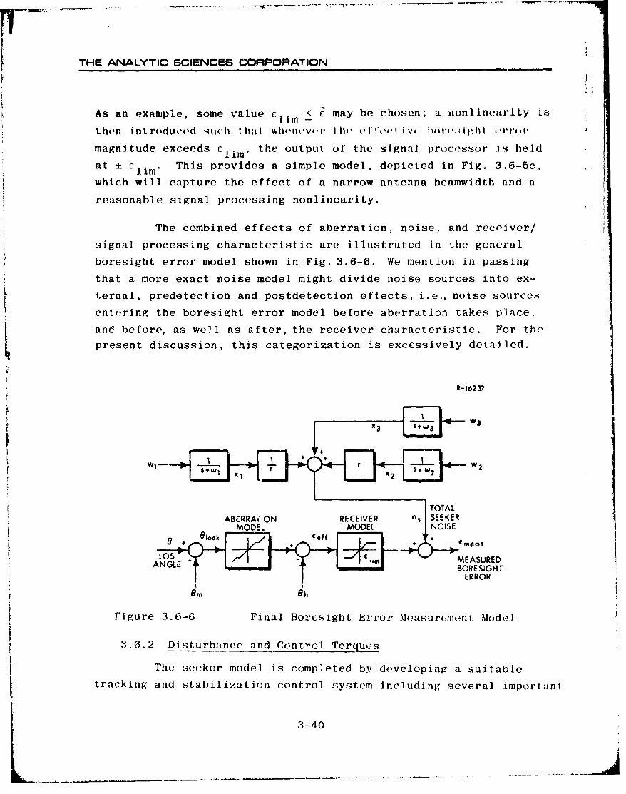
THE ANALYTIC SCIENCES CORPORATION
As an example, some value c C may be chosen; a nonlinearity is
then introduced suich that whollnevel Iho (4l'lIIcl iv',, Iw,,r ',ilh , Irr
magnitude exceeds c lim, the output of the signal processor is held
at ± E lim. This provides a simple model, depicted in Fig. 3.6-5c,
which will capture the effect of a narrow antenna beamwidth and a
reasonable signal processing nonlinearity.
The combined effects of aberration, noise, and receiver/
signal processing characteristic are illustrated in the general
boresight error model shown in Fig. 3.6-6. We mention in passing
that a more exact noise model might divide noise sources into ex-
ternal, predetection and postdetection effects, i.e., noise sources
entering the boresight error model before aberration takes place,
and before, as well as after, the receiver characteristic. For the
present discussion, this categorization is excessively detailed.
R-16237
x 3 ZIw3
TOTALABERRAi'ION RECEIVER ns SEEKER
MODEL MODEL ]NOISE
19 MOOS
LOS .1MEASUREDANGLE ,RE
BORESIGHTERROR
am 8
Figure 3.6-6 Final Boresight Error Measurement Mode[
3.6.2 Disturbance and Control Torque
The seeker model is completed by developing a suitable
tracking and stabilization control system including several imporlant
3-40

ITHE ANALYTIC SCIENCES CORPORATION
Ssources of' disturbance torque inputs. In terms of the inertially-* referenced angles f and i shown in Fig. 3.6-1, we can derive a
relation of the form
Ip I p =TC -Td (3.6-7)
pwhere I is the moment of inertia of the sveker head about thegimbal pivot, T is the external control torque (derived from an
F, electric servo motor, for example), and Td is the total disturb-
ance torque.* For the present discussion, consider three components,
T T + T + T (3.6-8)d m f r (.8
where Tm is an effective torque due to seeker head mass imbalance,
and we include two external torque components, Tf due to nonlinear
friction in the gimbal and Tr due to nonlinear restoring torques.Since the seeker head center of gravity is generally displaced
from the pivot point, as shown in Fig. 3.6-1 and specified by theparameters r 0 and 00P the moment of inertia I is related to the
j corresponding moment of inertia referred to the center of gravity by
S.- Ip I I0+ mr0 (3.6-9)
where m is the mass of the seeker head.
* S. The Pxternal torques due to spring vrnd friction effects
are modeled by the relations
Restoring Torque: Tr L f (O( -
I Friction Torque: Tf = f20h)
I where 0 h is the angle between the seeker and missile center lines.Often restoring torques are linear for small angle deflections,
a *The use of hydraulic actuators for mechanizing the seeker track-ing function generally leads to a quite different model of theseeker dynamics; we do not consider this case here.
3-41
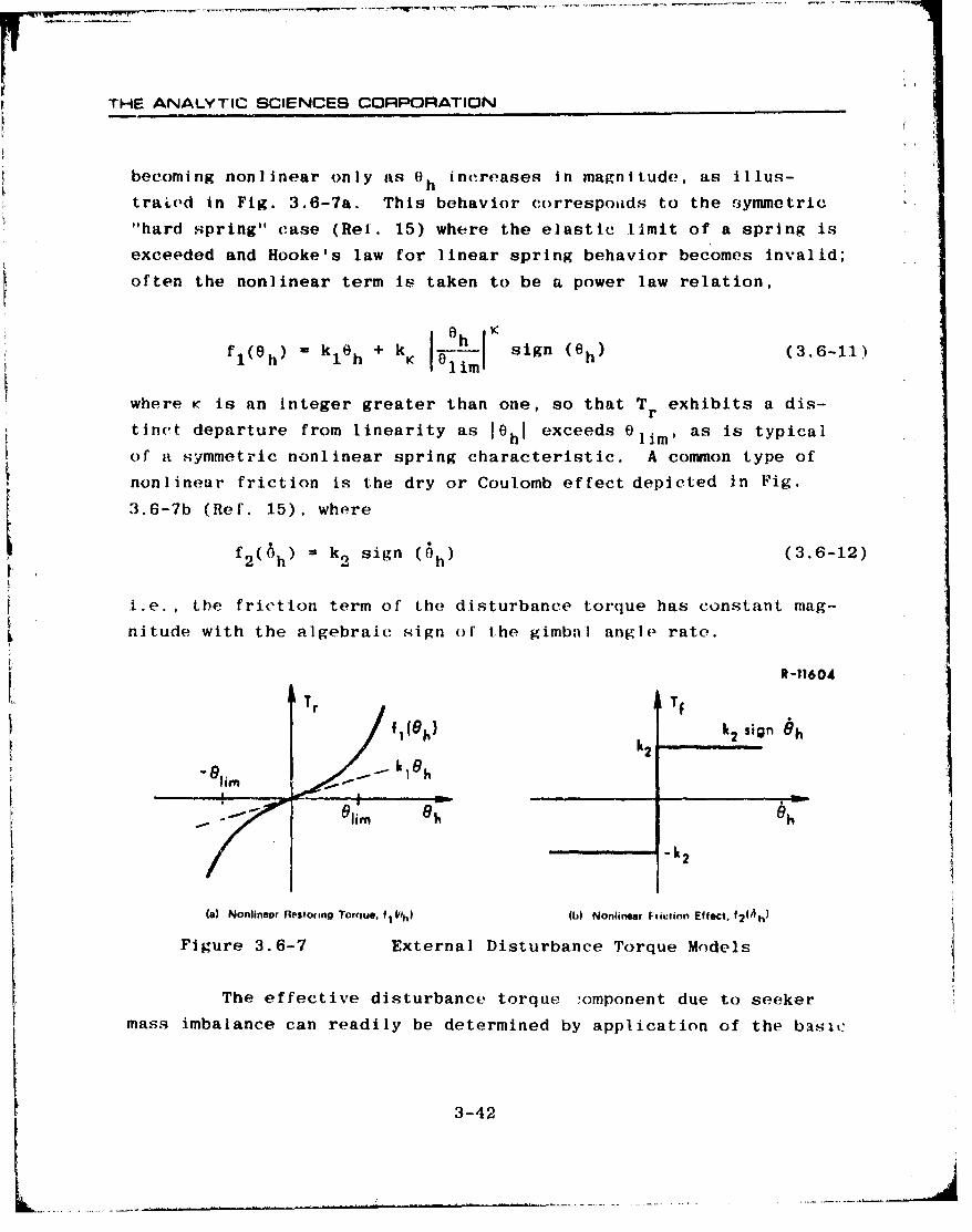
THE ANALYTIC SCIENCES CORPORATION
becoming nonlinear only as 0 increases in magnitude, as illus-
trased in Fig. 3.6-7a. This behavior correspoads to the symmetric
"hard spring" case (Ref. 15) where the elastic limit of a spring is
exceeded and Hooke's law for linear spring behavior becomes invalid;
often the nonlinear term is taken to be a power law relation,
fl(kh) - kl 0 h + k K sign (0h) (3.6-11)
where K is an integer greater than one, so that Tr exhibits a dis-
tinct departure from linearity as 16hi exceeds 0 lim, as is typical
of a symmetric nonlinear spring characteristic. A common type of
nonlinear friction is the dry or Coulomb effect depicted in Fig.
3.6-7b (Ref. 15), where
f2(6 h k 2 sign (6h (3.6-12)
i.e., the friction term of the disturbance torque has constant mag-
nitude with the algebraic sign or the gimbal angle rate.
R-11604Tr Tf
fk(86)k 2 sign 6 h
•'Gulm 6 h 9
-k2
Is) Nonlinear Restoring Torque, fl. h) (b) Nonlinear Friction Effect. f2(th)
Figure 3.6-7 External Disturbance Torque Models
The effective disturbance torque -omponent due to seeker
mass imbalance can readily be determined by application of the baslc
3-42
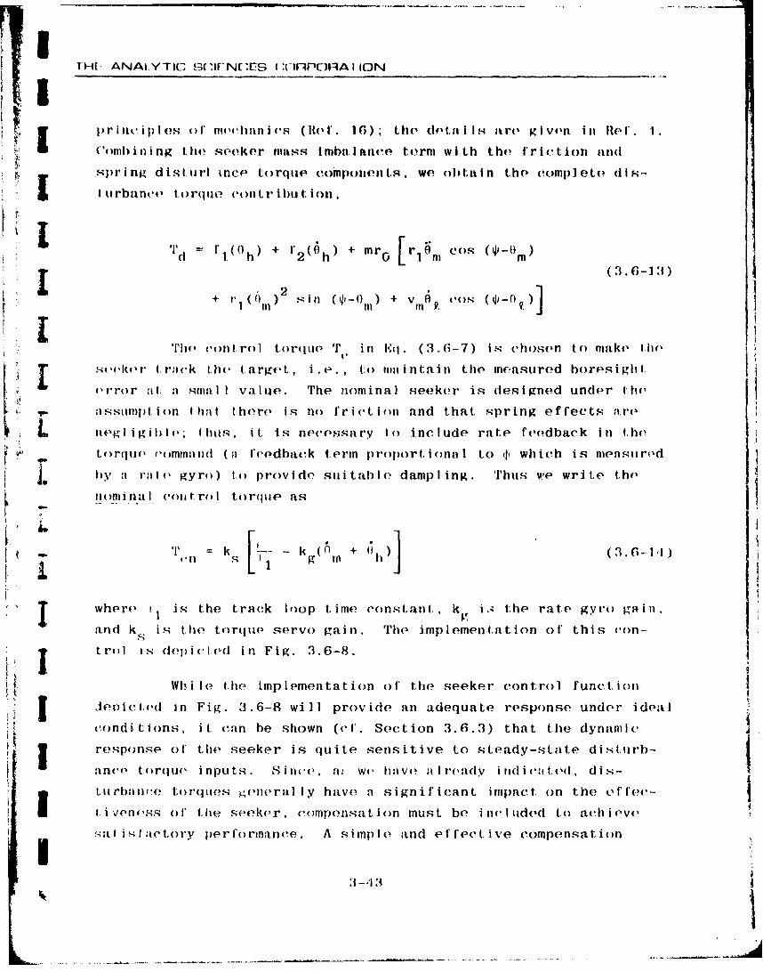
THE ANALYTIC -("NC(ES I(IRPORAI IONI1) r i it c i;)l, 1 s o I ' hanmo I (i (H l'. 16); theo I(,t.iti IIs utre g w I In !u[1(. 1.
Co(cmbin in ng I hv se ek er ma s I mba I atve tevrm wI th th cric tLion anid
spring disturl ince torque compolnen ts we W obtain the. complete dis-
Iturbanie torque conitrihution,
Td =rl(Oh) 2 '2-(h) + mro [r,6" cos (3.61m)
(3. 6-13•
+ (0) sin (q')-O) + Vm . e.-
T'lh' ('()n-.ro l tor(Ilo T i n lE:q. (3.6-7) is chosen t o make I. hoIVist-,,ke(r I rnck t.he target, i.e., I: o ma intain the mr, asured borvs ight.
orror at. a smal I value. The nominal seeker is designed under I h,a sstim .i ion that there is. no frieLi on and that spring effects are
inegligil ie; thths, it is necessary t o include rate feedback in t-he
to.rqu, co''mrnand (0a feedhack term proportio nal to (1, which is menasirod
by ia rite, gyro) to provide suitable damplingl. Thus we write th,
nominal ('olt r.ol tor(que as
J6
('_ T = k 5 [? k(O + (3 '1)
T where i is the track loop time constant, k i.; the rate gyro gain,
and k is the torquo servo gain. The implementation of' this v'on-
T t r I .N depict-ed in Fig. 3.6-8.
I. Wb i lle the implementation o)I the seeker control Functi on
S Jeoui cted in Fig. 3.6-8 will provide an adequate response under ideal
condi tions, it can be shown (v 1'. Section 3.6.3) that the dynami c
i' t response of thme seeker is quite sensitive to sLeady-stat.e di.sit,|rb- Ianco torque inputs. Sin ice, a w. ' havwe alrready indid:a t.e(I, di.-
trhatice torques gýenera~llIy have at significant impact on the feci'¢on(,.s of' the soeker, compensation must be inc luded to ahiove
-ýatislacto(ry iperfori anee. A .simple and effect ive compensation
3 -"13-%
!|I
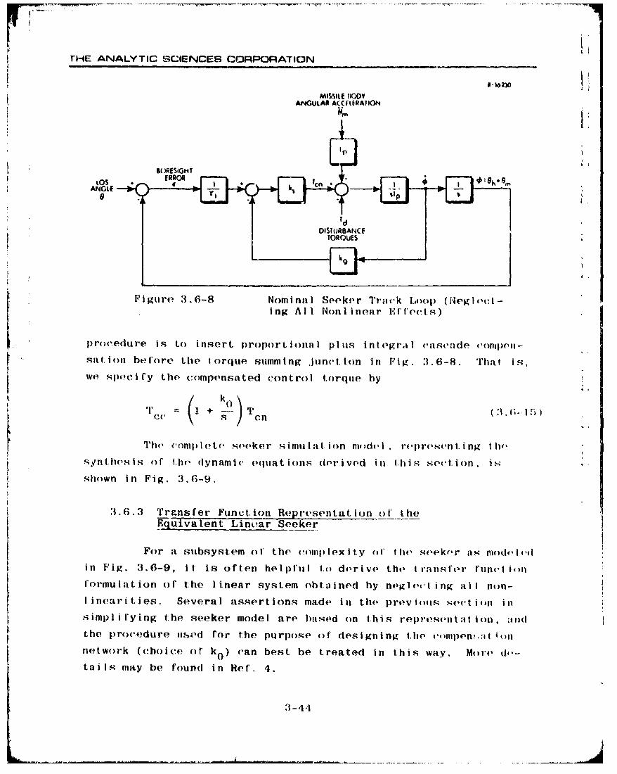
THE ANALYTIC SCIENCES CORPORATION
4-16230MISSILE IIODY
ANGULAR A( C II.IRATION
L O( R E . 0 : OH 0
Lo 1cn IANGLE ) 4
dDISTkURBANCE
TORQUES
Ftigtre 3 .6-8 Nominal Seeker Track Loop (|Eogloct -
Ing All Nonlinoar E r .ects)
pro•edure is to insert proport it nI I pl ius in lt.egral 1 o ,isende cof)l1)Cen-
sat.ion berore the torque summing .jiunctio(n in Fig. 3.6-8. That I s,
we s.•c•fly the compensated control torque by(k"Th' (,f•' ) mtlet , seoeker ,lniTiiA ation nOfol( dqI, r ,Iroc• n , i ng t h1
qyniti. hexis of 1he1 dynami(, equations dIvrivod in t.lhis soct. ion, I ,.
shown in Fig. 3. 6-9.
"1.6.3 Transfer Function Rep•,resentation ol' theEquiv'alent Linoar Seeker
For a subsystem oft the comp) Iilexity oI' thl, s.ee-ker ias fidolo'(l
in Fig. 3.6-9, it is often helpl'ul ho dorive the I ri'nslktr fun, 1i411
Formulation of the linear system obtained by neglecting all n)n-
lI near it. I es. Several assertions made in thl preyviiil; .wsct.ji(n in
simplil'ying the seeker model are hased on this representt:it ioni, al(Ithe procedure iise(I for the purpose oif designing tho c(•pvwlp'lI,:ii()nl
network (choice or ko) can best be treated in this way, Moro, d,-tails may be found in Hef. 4.
3-441
i i i • i / l l ........ .. .... . .. j.. .

THE ANALY TIC SCIENCES CORPORATION
£Ifeom K.wenotisc) ANI ROkAIH IN (J4A9A( I(PISIKI RAII (IO (,wd, 11're
II
Iy 1
I~ {.-z.~ Lii ~~* *,jJ~~j C I AI
am- * LCOj A,1 .A
4~
Vi I
F'i jti I( 3.63-9 (nvm)I etv See(ker Nb Ide I
10 31-45

THE ANALYTIC SCIENCES CORPORATION
We derine four inputs (relor to FIK. :3.6-10), V
k12 • In (3.6-17)
The trannsrer It'inetions d (S) to (14(,) l'or the ,(,Iiiivaluni bl(ok
diagram representation depicted in Fig. 3.6-11 ca ne Rh,'wn 1.() hv
k 2 + (13s [ I) 1 ]
S 3 +"ilZ3 + (12s + (I11
-k3 k 2 s 4 k1
i2 (s) 1 P[1 S . + (13,j2 + (12s + (ll] (:L.-18)
d, 1 (N) .- j dl(1S0)• ~ka
3
k3 sd Is + q3s (12s + (1
wl yre the ntum ri•rt ()r and deniominator vco 1'l'i ci Ients.,- :ir(' g ivon by
k1 + ks kj k0 k, k:1I)1 -- I i+ _2 --- 31+ 1- I I I
(3.6-19)k s k 0 k 3 k 2 k ks k
The, no)minal seeker i s do li !ed by a chi), ()I' 1paramintvor:
that I *nds t o acLcoptab lIe dynam Ic behavior in (huli abs(en ce 4i
3-46
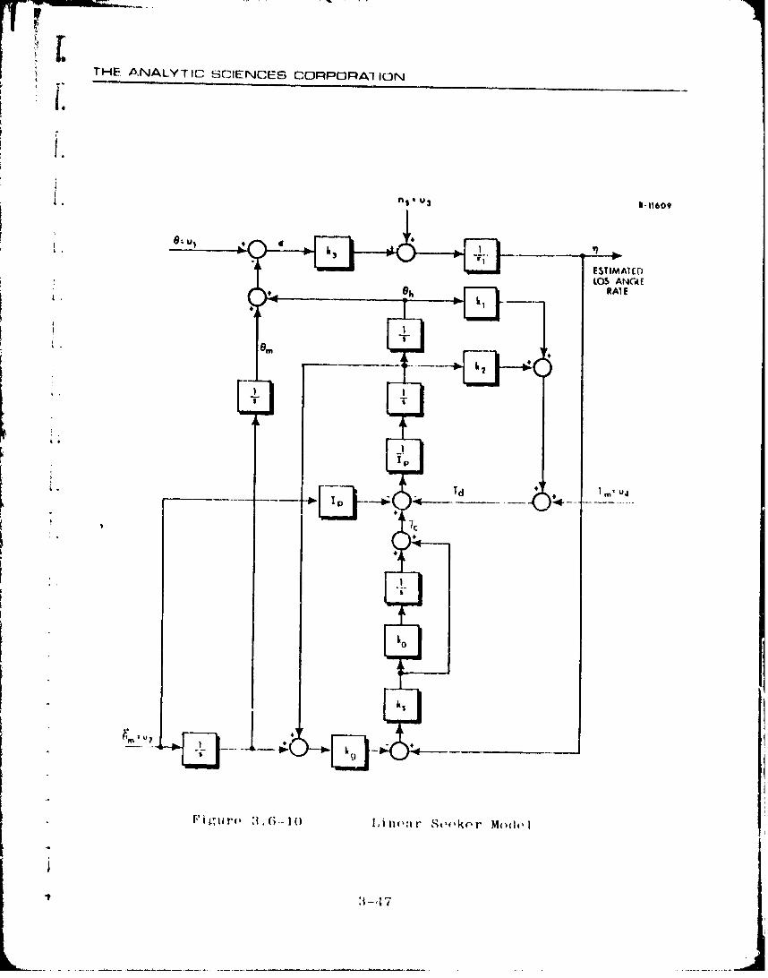
THE ANALYTIC SCIENCES CORPORAl ION
I.tI
fl1 ' U 3 I-11609
ESTIMATEDLOS ANGIE
RAI
d4
lip
Ito
ItsiFi gure' 3i6-10 ()i n tr ýSeeker Mode I
3-17
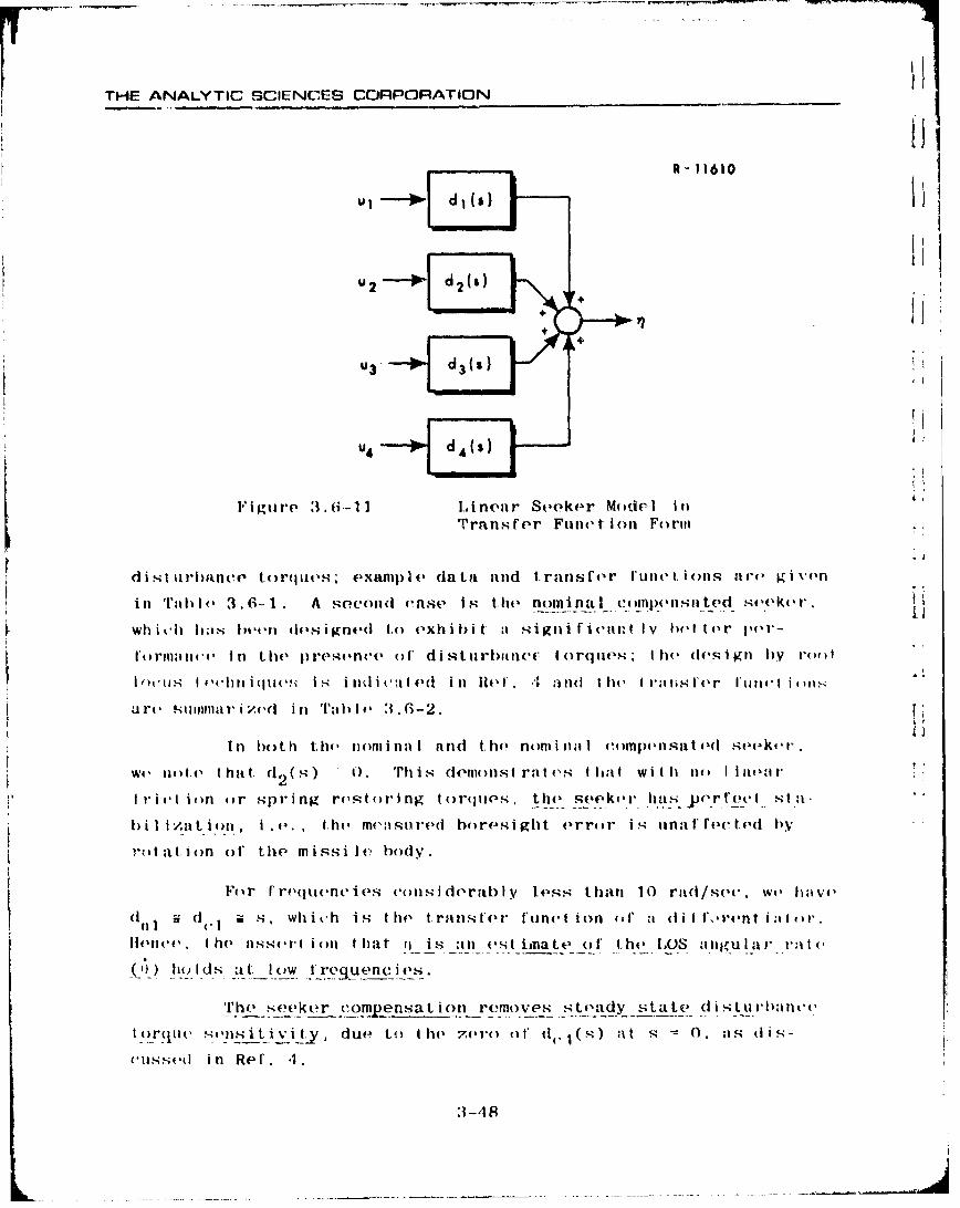
THE ANALYTIC SCIENCES CORPORATION
R - 11610
21 -~ 2(s)
Fig'il 3 '~ i.6(-11 Li near Seeker Model litTIran s fer Fuanct.i on Fo~rm
d ist urb'aince t( )rq ueo- examipl d '(a ta and trantsfer I tineti. i arvIe' gi1vvn
inl Tabh ' 3. 6.-1. A seetond (I se I s t.he nominaI l I c )ljompesitted ,4vveker,
wh I~i ch has heii'l tIE's igfl('( to ('xhi bi t. a sigiti f (i cantI Iv het I or petl-
lorinant'' in the pres-ncev (J di sturbatnec IorqIivm, Il( de1s i gn hy rwil
oci s 0411 I 'tjj i uc.' I-, i 1 lld t 'cid inIti U ' I. 4 andi lilt Irl'l s ber Itam 'Iic itiu-
art, comiiiar i ed in Tabo 3 i.6(-2.
fit 1)0)th t~ht riiornil I nid the fltmfl)i l comp('nsate ('IsePkt't'
we noteI that. (I () ,0. Trhis dernonst ratos t hat Wili Im h oII I'inot
Irit'jt' in ) r spring restori-ng toriltes. tesveekox ia eret Ii
1)1 1 'at. ion , i e.,. the mceastred hor-sight. error is5 ufat rvetedi by
r, at.ion of' the missi le body.
For F requenc ies 'oniisIderab Iy leiss than 10 raid/svee, we ha vt
1i (Ic s, whitIch i s tI(he I ransle'vr Ilun('t in oil4 ' a dI i I ','r'ntI lat o )r.
11ence , I he as'r t io that I ii - s an 11'st ina Le of t1.he LOS a niu Iitr rn t e
(Qi) holds at. low i'e~ (~liQs.
The seeker c omp~ensatI.ion remove., steady state i s Lurzbatice
torqua'c sonsitiv iy dlue to the 7t't'( oI' tI,.I(s) at s 0. ats d is-
cussed in Ref. I.1
:1-4 8
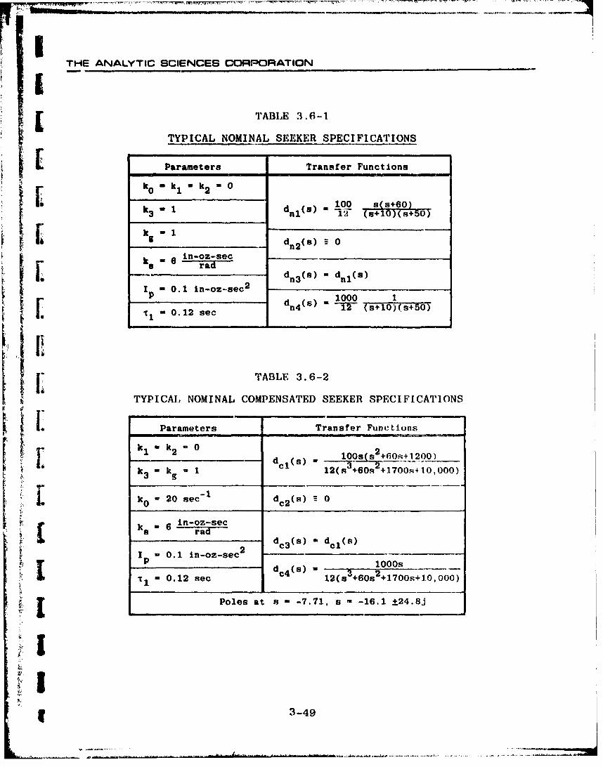
I- THE ANALYTIC SCIENCES CORPI=ORATION
[ TABLE 3.6-i
TYPICAL NOMINAL SEEKER SPECIFICATIONS
Parameters Transfer Functions
t -k I 2 0
100 88 100.
3 nl~)i 12(+10)s+50
dn 2 (a) 0
in-oz-seckd sad
Ip - 0.1 in-oz-sec2 n3 ( - d 1(s)
S1000 1dn 4 (s) - =0 (s+10)(s+59)1=0.12 sec
TABLE 3.6-2
TYPICAL NOMINAL COMPENSATED SEEKER SPECIFICATIONS
Parameters Transfer FunctionsK [ k 2 =0 2i = 0 i i2.k3 k I dcl(1008( lOss+60s+ 1200 )
kg I 12(s 4+60s+1700 S+1O,000)t3
k0 - 20 see- dc 2 (s) 0
in-oz-secSka 6 radxi dc3 (a) d del(F;)
1 w 0.1 in-oz-sec2
. dc 4 (s) 2T r-0.12 see 12(s +60s +1700s+i.,000)
i[ Poles at a -7.71, s - -16.1 ±24.8j
I3-49

THE ANALYTIC SCIENCES CORPORATION
3.7 SYSTEM MODEL. SUMMARYy
An example of' a complete missil -tnrge,. Int.erc(,pt. modolis portrayed in Fig. 3.7-1 with representations ,F all ol" 1.hev
subsystems described in the previous section:i npproprintoly
interconnected. This particular system model wns ext(insively
analysed in an investigation of the accuracy and efficacy or CAD)E'T
in evaluating the impact or variouis random and nonlinear eFrrects
on the performance of missile guidance syst(ems In Rel'. 4. As
indicated in previous sections, there are many assuinmp.ions behind
this I'ormulation; the system depicted in Fig. 3.7-1 Is intended
tu be demonstrative of the large class of problems that may be
considered in this realm, and not to be all inclusiv,.
All of the state variables aro depicled ,x(,(,cpt angle or
attack, t, control fin deflecti Ion, 6, and tIhe s•oeker state re-.quired t~o implement proportional plus integral compo||sat.icon, F,,I.
(3.6-31); thes•e states are enco)mpass•ed in thf- litkent dynamics,
r:oprosnted by t~he transfer functions gl(s), 2 (Fig. 3.4-3),and(I (+k0/s). For co)nvenient reference-., wo list t~he no)nlin,:ari-
ties incorp~orated in this particular system model t-nd indic'ate
their form:
•Seeke.r head restoring torque
fl1(0 h) k I 10 h I sign ( h)ri-
* Seeker gimbal friction
2 = k 2 sign ( 6 h)
* Receiver/signal processing characteristic
(F'I,3(•) =3Cli Sign(F:) , l'
I nim
3-50 J

.I- ,,1 ... . . . . . ,,,, .... . . . '-
THE ANALYTIC SCIENCES CORPORATION
l tI .V Pl'"t"l;" . . , , - I ,.,,,,,l ,,,, , A'1, fi ;-.1,1 -f .,S, ,,,1A,,-A
I A- FOAl,1r." --1 - - ., .
JJ
' t I SI •I ,, I lt
Rag deenen noises
I 1 I / 2. I
L _ _ - - T -. .. . . .' I
.. . . . lI I I l ,I v
'" MA5 "•
n + x 3X x +2
Seeker mass imbalance torque
STm mrO [rlUm (.o)s(I0h+00) + r, sin (0h+0O)
3-51.

THE ANALYTIC SCIENCES CORPORiATION
* LOS angio ('aliUlation
In- tan (y/x)
* Range calculation
r /x + y2
* Velocity resolution
X = -V cos(0() v cVos (()amt a
Y Vm -gin (60z + Vt sin (0a)
* Acceleration command limiting
nd oning itc~§2 max a(, J)"InX ~ at
" vt )s( V os ) +0)) + 0'a . n .v +
This chapter presonts an overview or modeling it.k ,
a rise in conside(lring t hp missile-t.:.rgot. int.eree I. pr(l)hIem. RM") I-
ist ic, rI(-Ireen taions for a var i vt y of non 1 i near v rlevc ts have ben
given, both to provide f ready roe'(rence for futI. ure sti.dioes orI1
tactical missile performance and to fac i tirate model developiwmnt
in other ar.as. The material i.s intended to guit(Je Ihew Usor iII
developing mathematical models appropriate for annlyzing missi I
syst~ems using CADET.
3-52

ITHE ANALYTIC SCIENCES CORPORATION
I
S4. JU ASI-LINEARIZATION: PRINCIPLES AND PROCEDURES
i 4.1 CADET AND STATISTICAL LINEARIZATION
[ To review the fundamental equations or CADET derived In
Section 1.2, Eqs. (1.2-6) and (1.2-7), the differential equntionm
_ = f + Gb
L P -NP + PNT + GQGT (4.1-1)
govern the approximate evolution of the mean vector and covari-
ance matrix of the state variables,
ITI r= E [ix] (4.1-2)
P = E [(x-m)(x-m)T]
where the state vector differential equation is nonlinear and time-
varyi ng,
x - f(x,t) + G(t)w (4.1-3)
I F.'quation (4.1.-I) involves the vector f and matrix N which are
de f i ned by
f E [ f(x,t)]
ri I"-x-e)T3P-1(4.1-4)
•I N = E [l(x.t)(x-m)T] (414
Analytic expressions for C and N in Eq.(4.l-,l) can be de-
termined only if the form of the joint probability density function
q 4-1
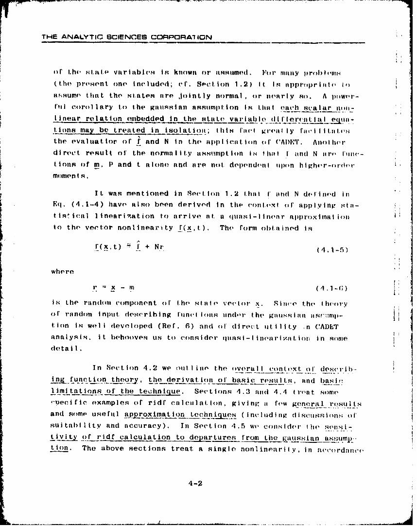
THE ANALYTIC BCIENCES CORPORA7 ION
(o Ihe st. at- variublb,- Is known or IamHmimedt. For mlany probI)rlems(the present one Inc luded; Cf. Sectioton 1.2) It. is applropt-irl te i.)
ati.umv that the st.tates are Jointly normal , or niearly so. A I)t)wf'r'-
|'Il corol lary to the gausslIan nassuiml)t Ion Is tiha vt('ach scaalar tmi-
linear relat ion embedded in the state var iabl) I(lle_ .nt liii ( lii.-
t. ions may be treated in isolatIoni; th is I'niv l greal I I y Ia4'. I it t1,1.4
the evaluat tor or f and N in the appli c|it .ion or ('Ai)EI' . Anol. hrr
direet result ol' the normality ussurnpt ion i s Ihl I I and N iir, f'[inc,-
tions of m, P pand t ailIon; and areV not. dependvdn t ii jfn h i.ghe r-o i'df, r
momen I s.
It. was mentioned in Se.t.lton 1.2 that I' iuind N dflilned In
Eq. (4.1-4) have also been derived In the contelxt of applylng sita-
t~i, s (ca11 1 lnearI, at ion to arrIvrf atI a qu(si-I I nenr approxtinat ioto the vector nonlinearity _f(xt.). Thte form obtained I.s
'(x,t) C + Nir (4.1-5)
where
-r = x in,( 1 . - ;
Is Lhe randohim component ()o' the s tate., vecto.r x. Sinac * e the I.heryo r random Inplut desc ribing l'unet ionos undor thhe gitussIan tiisnf-ip- Vtiton is well developed (Ref. 6) and o1 (tirtact utt.i lity .n CADET
analysis, it behooves us to consider (In si-linearizat.orto in qonl(-
(teta 1I.
In Sect ion 4.2 we outl, lin the vterall .cont.xt. (I" des,'ih--
Ln.k function theory, the derivation ol' basic. results, and basif-
limitations of the technique. Sections 4.3 anid 4.4 tr(at some
rF-eciftc examples of ridf calcualtiton, giving a few general resultsand some usefut I.approxLmation tcchniLou.e (Inc, I d I g disISS i (,; of
suitability and accuracy). In Section 4.5 we consider Ihe sonlsI-
tivity of rtdf calculation to departures from the gius-sian assump -
tion. The above sections treat a single nonlinearity, in ftccordance(,
4-2
'. .' . - - _ . . - - - - -- - - -- - - - -- -- - - . . .
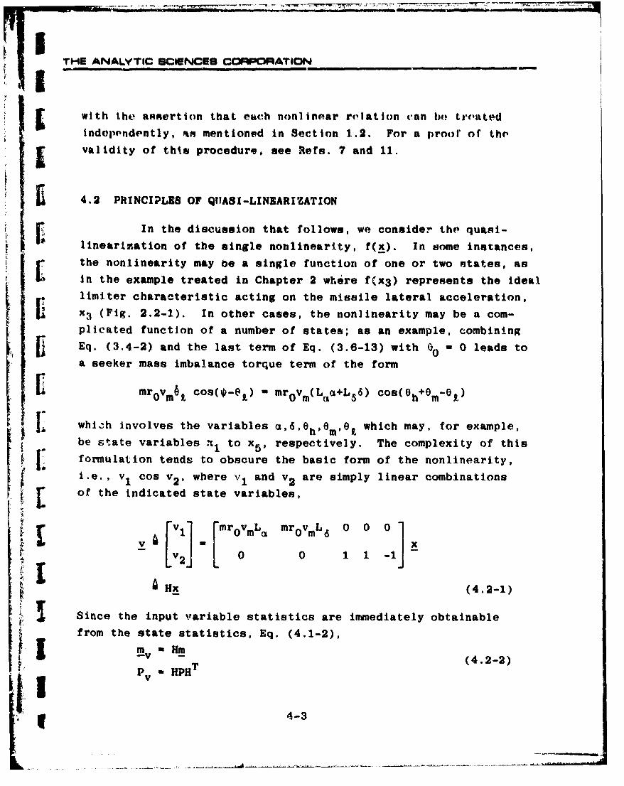
THE ANALYTIC SCIENCES CO 0RF:OATIONiK I|lu .. ~--II1_ --
with the assertion that each nonlinear rlation van b1 trated
indoepndently, an mentioned in Section 1.2. For a proor or the
validity of this procedure, see Refs. 7 and 11.
4.2 PRINCIPLES OF QTIASI-LINEARIZATION
r In the discussion that follows, we consider the quasi-linearization of the single nonlinearity, f(x). In some instances,the nonlinearity may be a single function of one or two states, as
in the example treated in Chapter 2 where fix3) represents the ideallimiter characteristic acting on the missile lateral acceleration,
x 3 (Fig. 2.2-1). In other cases, the nonlinearity may be a com-plicated function of a number of states; as an example, combiningEq. (3.4-2) and the last term of Eq. (3.6-13) with o - 0 leads toa seeker mass imbalance torque term of the form
- 0 mroVm6 cos(*-e-) I mr 0 vm(L M +L 5 6) cos(eh+OM-0g)
whiLh involves the variables a,6,6 h)(mIe which may, for example,
be state variables % to x., respectively. The complexity of this
formulation tend& to obscure the basic form of the nonlinearity,i.e., v1 Cos v2' where v 1 and v 2 are simply linear combinations
h[ of the indicated state variables,
V -
Since the input variable statistics are immediately obtainable
from the state statistics, Eq. (4.1-2),
I- Hm (4.2-2)
I v -HPH3
t 4-3
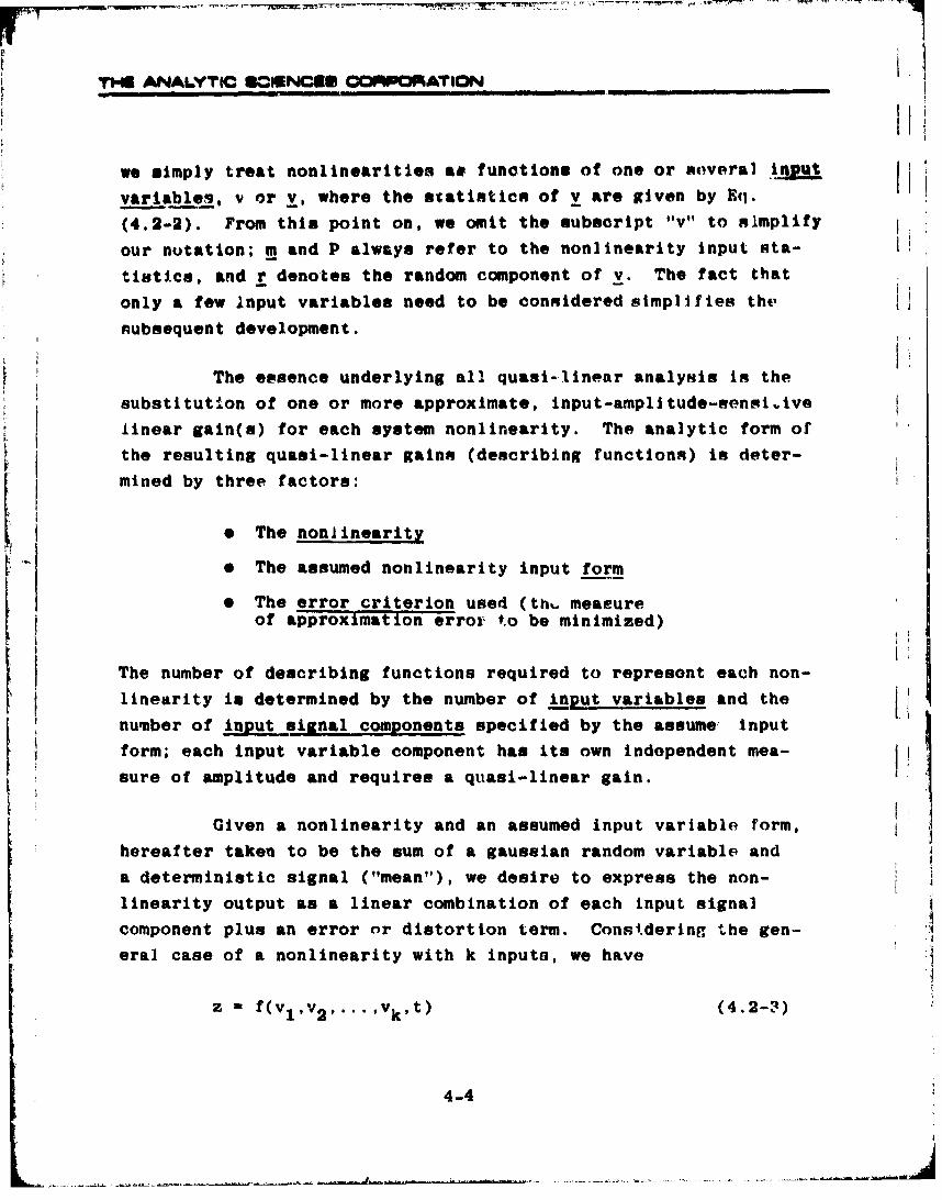
THE ANALYTIC C•HIENCE.S 1"0N01rAT ION
ii
we simply treat nonlinearitles as functions of one or smveral .iAut
variables, v or v, where the statistics of v are given by Eq.
(4.2-2). From this point on, we omit the subscript 11v" to simplify
our notation; m and P always refer to the nonlinearity input eta-
titices, and r denotes the random component of v. The fact that
only a few Input variables need to be connidered simplifies the
rubsequent development.
The essence underlying all quasi-linear analysis is the
substitution of one or more approximate, input-amplitude-seni.tive
linear gain(s) for each system nonlinearity. The analytic form of
the resulting quasi-linear gains (describing functions) is deter-
mined by three factors:
* The nonlinearity
* The assumed nonlinearity input form
o The error criterion used (th, measureof approximation error to be minimized)
The number of describing functions required to represent each non-linearity in determined by the number of input, variables and the,
number of input signal components specified by the assume input
form; each input variable component has its own independent mea-
sure of amplitude and requires a quasi-linear gain.
hereafter taken to be the sum of a gaussian random variable and
a deterministic signal ("mean"), we desire to express the non-
linearity output as a linear combination of each input signal
component plus an error or distortion term. Cons.dering the gen-
era] case of a nonlinearity with k inputs, we have
z f(vl,v 2 ,... ,vk,t) (4.2-q)
4-4

THE ANALY'IC SCIENCES CORPORATICN
S[ for which we seek an approximation of the form
z t z0 + bTr (4.2-4)
where z and b (a vector of dimension k) are to be determined.*
Based on the desired form if the quasi-linear approxi-
mation, Eq. (4.2-4), we consider the mean square error,
E E[ z - z0 o biri} (4.2-5
Setting the partial derivatives of the mean square approximationerror with respect to z and bj equal to zero gives us the set of
necessary conditions for minimization,
ao 2E f -zo bjrj(-l) 00 TI.
2Ef. b r4l(-rj)] M 0, j W-,,.,I [b 0 Jul
(4.2-6
Taking the indicated expected values term-by-term reduces Eq.
(4.2-6) to
Szo M E [f
(4.2-7)
bI bTP - E [f r T]
I IThe first term in Eq. (4.2-4) could be expressed as aTm, i.e., alinear combination of the means; however, we note that the elementsof a can only rarely be found explicitly, as can be appreciated inthe example of Eq. (4.3-34).
I4-5
TH ANAi,,YTI SO RNIMO•..•I CO WK IIATIO•N
where we have expressed the results in their more compact vector- flmatrix form.
Comparing Sq.. (4.2-2) and (4.2-7), we have
f(v,t) 8 E If] + E f r P1
A + n r (4.2-8)
which is identical to the scalar case of Eqs. (4.1-4) and (4.1-5).
To see that the above solutions do indeed lead to mini-mum mean square error, we observe that H4
S22- 2 > 0
*az 0
a-Cb2 - 2 F r2] > 0, j - 1,2,...,k
which are sufficient conditions for the existence of a local mini-
mum.
In evaluating the expected values needed in Eq. (4.2-8)we invoke th3 assumption of joint normality to write (Ref. 11) L
- [(2 )klpl] oxp r' Pr (4.2-9)
By definition, then
(2r kA f(v~t) exp- 1 (X-m) T1(V-M)?
dv 1 dv 2 ''" dvk (4.2-10)
4-6
THE ANALYTIC SCIENCES CORPORATION
To aid in evaluating Ln, we form
A
(if
,, /,)T f•. k ]'•' S rpI_kp A '~ af 1 -x -
_m {32 [ (21n IPIJJ... f(v't) exp - r P rT P r
dv~dv 2 -, dv k
LmkiP- E lf(v,t) r] (4.2-11)
which demonstrates that tho second relation In Eq. (4.2-7) under
the gaussian assumption is identical to*
n -=--f (4.2-12)
which is the scalar version of Eq. (1.2-10). After f is calcu-
lated according to Eq. (4.2-10) for utilization in Eq. (4.2-8),
the random component describing function vector n usually may be6. P
obtained much more easily using Eq. (4.2-11), than by direct solu-
tion ot Eq. (4.2-8).
From the development outlined nbove, we nult that the
use of describing functions provides an approximation to nonlinearphenomena that retains input-amplitude sensitivity through the
T dependence of ? and n on m and P. In CADET, the usefulness of thequasi-linear approximation, Eq. (4.2-8), lepends on the validity
of the gaussian assumption on x. The accuracy question is a very
complex issue -- probably, an unresolvable one in a general,
N()tt, that by convention the derivative of a scalar by a columnvector is a row vector, and, by extension, the derivative of a
column vector by a column vector is a matrix.
4-7
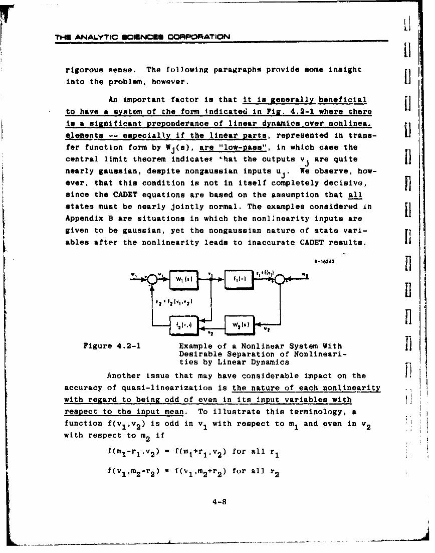
LITHIMi ANALYTIC IICIENCES COIRPORATION
rigorous nense. The following paragraphs provide some insight Iiinto the problem, however.
An important factor is that it is generally beneficial 11to have a system of the form indicated in Fig. 4.2-1 where there
in a significant preponderance of linear dynamics over nonlinea.
elements -- especially if the linear parts, represented in trans-
fer function form by Wj(s), are "low-pass", in which case the
central limit theorem indicateE 'hat the outputs v are quite
nearly gaussian, despite nongaussian inputs u . We observe, how-
ever, that this condition is not in itself completely decisive,
since the CADET equations are based on the assumption that all
states must be nearly jointly normal. The examples considered In j]Appendix B are situations in which the nonlInearity inputs are L!
given to be gaussian, yet the nongaussian nature of state vari-
ables after the nonlinearity leads to inaccurate CADET results.
R- 16243
Figure 4.2-1 Example of a Nonlinear System With 11Desirable Separation of Nonlineari-ties by Linear Dynamics
Another issue that may have considerable impact on the
accuracy of quasi-linearization is the nature of each nonlinearty.
with regard to being odd of even in its input variables with Irespect to the input mean. To illustrate this terminology, a
function f(vlv 2 ) is odd in v 1 with respect to m, and even in v 2
with respect to m2 if
f(m l-r lv 2 ) = f(ml+rlv 2 ) for all r,
f(vl,m2 -r 2 ) - f(vl,m2 +r 2 ) for all r2
4-8
THE ANALYTIC SCIENCES CORPORATION
For the rest of this discussion, we conpider the zero-mean case,
and refer only to oddness and evenness since the extension tc
non-zero means is obvious.
It is beneficial to have single-input nonlinearities
which are odd functions of their inputs. (Section A.1 contains
a comprehensive catalogue of ridf's for this basic type of non-linearity,) In contrast, even nonlinearities must be considered
with caution. It is simple to demonstrate that the random com-
ponent gain, n, is identically equal to zero when f(v) is an
even function of a zero-mean input v; this condition generally
provides an inadequate approximation.
T-I In treating multiple-input nonlinearities, the situation
becomes mere complicated. Let us consider a few examples: first,
f(vl,v 2 ) = VfVl + nlrl + n2 r2
Sf=mm2 P 2 2
n1 =m 2
n 2 =m 1
where the indicated quasi-linear approximation has been derived inRef. 3. In a zero-mean situation, the quasi-linear representation
degenerates to a single mean component* given by P 1 2 ' the cross
correlation of v 1 and v 2 . By extension, any two-input relation
of the form"' ,V2) f~f(vl ,od(l 2
,v2) = flodd(vl) f2,odd(v 2 )will have zero random component describing functions when vI andS2 have zero means, which will generally lead to unsatisfactory
. results. Next, we consider
f(vlv 2 ) = V f + nr + nr
L *We observe that the quasi-linear approximation, Eq. (4.2-8),always conveys the mean input-output relation correctly.
4-9
; 1t-/-

THE ANALYTIC SCIENCES CORPORATION
-[im+P 2 2) + 2m2P12 )]
n 1 W M2 + p22
n 2 -f Lm1m 2 + P1 2 )
which can be derived using the general result given in Eqs.(4.3-22),(4.3-32), and (4.3-33). Here, in the zero-mean input case, we have
no output mean and non-zeru random component gains for both r1 and
r 2 , provided p1 2 and P2 2 are non-zero. Thus in general it would
seem that two-input relations of the form
f(vl,v 2 ) = fl,odd(vl) f2,even(v2)
are advantageous from the point of view of describing function ap-
proximation accuracy in the zero mean case. Finally, using the
result in Eqs. (4.3-39) and (4.3-40),
f(vl,v 2 ) = v1v 2 . f + nlr 1 + n2 r 2
A= 2 2f = (m1+p1 1 )(m2 +r 2 2 )+2p 1 2 (P 1 2 +2mlm2 )
n = 2ml(m2+P2 2 )+4m 2 P1 2
2n2 = 2m2 (m1 +P 1 1 )+4mlP 1 2
Again, there is no random-component transmission (nfnfin=) in thj
zero mean case, so the nonlinearity form
f(vl,v 2 ) = fl,even (v1 ) f 2 ,even(v 2 )
is apt to give poor results in this situation. As in the discus-
sion of single-input nonlinearities, these comments may be di-
rectly extended to the non-zero mean case.
The preceding paragraphs considcA bhe accuracy of quasi-linear approximation for a number of nonlinearity types. The
problem that often arises is "zero transmission" of one or more ran-
dom component(s); the basis of this phenomenon is that the random in- V,put describing function n in the quasi-linear approximation, Eq.(4.2-8), only captures that random component of the nonlinearity out-
put, z,which is correlated with the input variables, in the sense that
4-10
THE ANALYTIC SCIENCES CORPORATION
IE C~rjz] 0
I How serious this effect is on the overall accuracy of CADET Ishighly dependent upon the complete system model; it may be that
if the random effect which is neglected by the quasi-linearization pro-
5 cedure is truly insignificant, in the sense that other linear or
nonlinear dynamics may dominate. In this eventuality, the useful-
.1 ness of CADET is unimpaired. On the other hand, it is a straight-
* forward exercise to fabricate simple examples where a CADET analysisL ~would be totally incorrect -- cf. Appendix B. A loose but usefulanalogy can be drawn between the relation of describing function
r accuracy to the validity of the complete quasi-linear system model- (in particular, to the accuracy of CADET analysis) and the parameterr sensitivity problem in linear systems theory (in particular, the re-
r lation between the accuracy of standard covariance analysis, Sec-
r tion 1.1, and imprecision in knowledge of -the linear gains of theIi system model). In the parameter sensitivity problem, an inaccurate
ally no effect on the overall system performance (in the low sensi-
tivity case), or it may make the model behave in a completely dif-
~ ferent manner than the system (in the high sensitivity case), ren-dering the model meaningless. Thus in assessing the usefulness ofPiE CADET in a given situation, one must use insight and experience inorder to evaluate the approximate accuracy of the describing func-tions used and the relative importance of their inaccuracy.
The preceding comments on the significance of oddness andevenness should provide some useful guidelines in estimating the
accuracy of various ridf's. The results outlined in Section 4.4r also provide a good qualitative "feel" for the inaccuracy in de-L scribing function calculations that arise from the departure of theIL[ nonlinearity input from the gaussian assumption. We emphasize that,
because CADET is an approximate technique, it should be comparedwith monte carlo simulations in a few selected cases, to verifythat CADET accurately captures the nonlinear effects under con-sideration (refer to Fig. 5.2-2).
4-11
THE ANALYTIC SCIENCES CORPORATION
4.3 RANDOM INPUT DESCRIBING FUNCTION CALCULATIONS
4.3.1 Single-Input Nonlinearities
In obtaining a quasi-linear representation of a nonlinearfunction of one variable (v) under the gaussian assumption, we
have
f(v) - f + nr (4.3-1)
where Iii
mm E IV]
r v -m
p = o2 = E [r 2 ]
2(4.3-2)A 1 2(v_ )
f( f(v) e dv
2podm n2-0 3 (v--) f(v) e dv
Since the catalog of random input describing functions (ridft s)provided in Appendix A is not exhaustive, the following detailed
sights into the development of describing functions for other non-lineerities. F•
As a general observation, it is often advantageous to iuse a linear transformation to simplify the exponential functionin Eq. (4.3-2); the change of variable
4-12

mTHE ANALYTIC SCIENCES CORPORATION
yields
A 1 u2I if m .1 _ f(au+m)e du (4.3-3)
Further simplification may result by eliminating all terms in f
that are odd in u; for example
n[a0+a1u+a2u2 +---] e• du - 0 +a2u2+au 4+...] - f <, du
11 ~ ~ G 1 2 u(43)
Sfoau+m~e du - SO00 f ev(au+m)e 2 du(434
where the even part is given by
fe v(u+m) -1 [f<au+m- + f(,<au+m)] (4.3-5)
After this procedure has been carried out, the following integral
C evaluations often prove to be useful:
1u2
o e- du = 1!/2 -Tr - ,,
--u2
S • ST u< 1 ,,, 2 ,, . • • °
S1 u2ko 2
S_ k du = (1)(3)(5)...(2k-1), k > 1
4-13

THE ANALYTIC SCIENCES CORPORATION
2These results and others involving the integrand factor e- u
may be found in any complete tables of definite integrals; cf.
Ref. 16.
Example 1: Using the above relations, we can obtain thequasi-linear representation of the nonlinearity v3 by inspection.From Eq. (4.3-3)
A M E [v3] %. (au+m) 3e- Vdufh/2-ir
Dropping terms that are odd in u yields
f 1 . m3 +3mo2u2 e du
so application of Eqs. (4.3-6) and (4.3-2) results in
f =rm + 3mo 2
(4.3-7)Bf m2 02".n= -= 3(m + 2)
Example 2: Trigonometric nonlinearities may be treated
conveniently using the above techniques in conjunction with com- '
plex variable notation: recall that the complex function eiv is
of the form
f(v) = eiv
= cos v + i sin v (4.3-8)
so we have
1 (_7m)2exp iýd2_ a - ( )
Adding and subtracting (- a2+ im) in the argument of the ex-
ponential function permits us to complete a square;
4-14
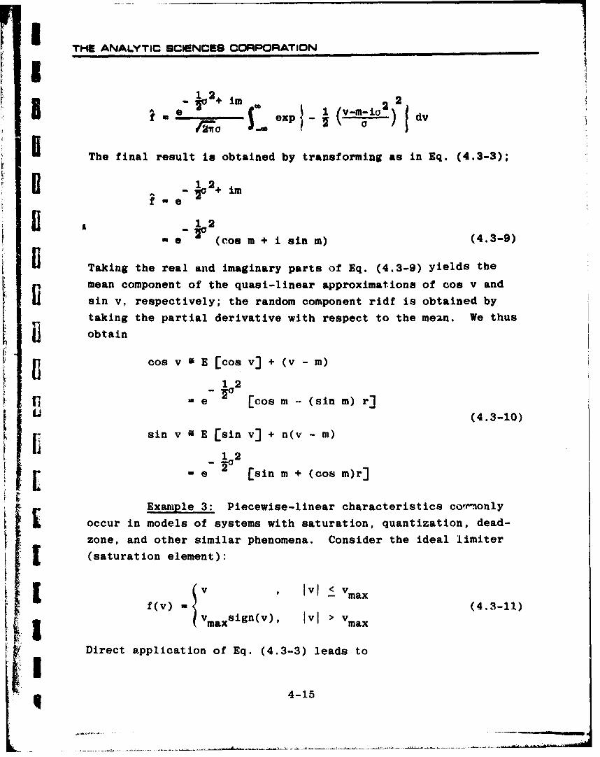
THE ANALYTIC SCIENCES CORPORATION
2+ im
I The final result is obtained by transforming as in Eq. (4.3-3);
£~ 12(con m + i sin m) (4.3-9)
I Taking the real and imaginary parts of Eq. (4.3-9) yields the
mean component of the quasi-linear approximations of coo v and
sin v, respectively; the random component ridf is obtained by
taking the partial derivative with respect to the mean. We thus
obtain
cos v E [cos v] + (v -m)
K i e- ecos m (sin m) r]
(4.3-10)
sin v 9 E Esin v] + n(v - m)
1 2
-e [sin m + (cos m)r]
Example 3: Piecewise-linear characteristics comreionly
occur in models of systems with saturation, quantization, dead-zone, and other similar phenomena. Consider the ideal limiter
(saturation element):
f(v) = V a (4.3-11)
vmax sign(v), IvI > vmax
Direct application of Eq. (4.3-3) leads to
4-15
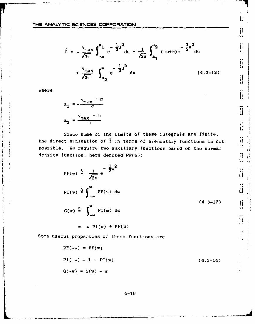
THE ANALYTIC SCIENCES CORPORATION
a1 12 a 12S- I e xdu + (ou+m)e du
4.--max e- du (4.3-12)
where
Vmax
a 2 maxS°Li]
Since some of the limits of these integrals are finite,
the direct evaluation of f in terms of eietnentary functions is notpossible. We require two auxiliary functions based on the normaldensity function, here denoted PF(w):
1.2A 1 •Pr(w) - e •
/-wf
P1(W) PF(w) dw
(4.3-13)G(w) A=IoPI GO dw
'-00
= w PI(w) + PF(w)
Some useful properties of these functions are
PF(-w) = PF(w)
PI(-w) 1 - PI(w) (4.3-14)
G(-w) = G(w) - w
4-16
..
ITHE ANALYTIC SCIENCES CORPORATION
lim PF(w) - 0
1im PI(w) - 0, l1m P1(w) - 1 (4.3-15)
Inm G(w)-O, 1im G(w) lim w-o
The mean ridf term f (Eq. (4.3-12)) can be manipulated directly
to obtain
f -a G i (4.3-16)
From Eq. (4.3-13) we have that
S~dGWG - PI(w)
iiso by inspection the random component gain is
ak vmax +m (mxm(.-7
1 1 L1 nn -P (--17)2 -n - P- - aPl + P 1 1 (4 .3 - 7
E The functions in Eqs. (4.3-13), (4.3-16) and (4.3-17) are
standard in several works (cf. Refs. 6 and 18). Other references
[ (cf. Refs. 15, 17) use the error function,
Serf(w) e- 2 du (4.3-18)
which is related to the probability integral PI(w) by
I erf(w) - 2PI(/2w) - 1 (4.3-19)
Since the error function is available in some computer scientific
subroutine packages, it may be advantageous to use
4-17

r=....1 ......... (.. .... 1 [THE ANALYTIC SCIENCES COR::PORATION
" e1 1 +..(... (.1.3-20)
This result and many other descrtbtng function representations
for a variety of piecewise-linear functions may be found in
Ref. 6; basic examples are given in Appendix A.
4.3.2 Multiple-Input Nonlinearities
As might be anticipated, the describing function deriva-
tion for functions with multiple inputs becomes more involved
than for the single-input ci,.se. In general, for two variables
"we seek'' f(vv2) - + nlr 1 + n2 &2 + JTr
where
L U
P"1 J 2 02 EA2
L 1 2 2
1 f (v,v 2 ) e- dvldv2 (.2
•,• (4.3-21)
A
4-18

THE ANALYTIC SCIENCES CORPORATION
I To demonstrate evaluation of integrals of this form, we
consider the following general form of two-input nonlinearity for
i which we derive a useful new result:
Cae 1: For a nonlinearity that has a linear factor in
one variable,
f(vlv 2 ) - Vlg(V2 ) (4.3-22)
we write Eq. (4.3-21) out fully to obtain
f dva vdv2 2ex
, zml\/v%-m2\ v2 =m 2)2]1 dl (4.3-23)
r It would be possible to integrate this equation with respect to
v 1 directly, making use of the relation
, u exp (-vuu2 +2vu) du =/ev (4.3-24)
(Ref. 17). However, a more systematic approach, explained below,S~reduces the possibility of error in the manipulations and algebra
involved in evaluating f. (The same technique is indispensable
for three or more variables.)Ccnsider the argument of the exponential factor, rTP-1r;
we seek a linear transformation w - R-r which simplifies the
integrations of Eq. (4.3-23), Choose the matrix R to be
... . R 2 (4.3-25)
40 2
S~4-19

THE ANALYTIC 64CtENCES CORPORATION
.o Iiso) by clef inition 1
P - RR T (4.3-26) [Defining w to be given by
W -1
vi-mr v2-m2a, /1_- " P(4.3-27)
v 2 -m2
a 2
we obtain :I(r)T P(-1 n w- (4.3-28)
This change of variables in Eq. (4.3-23) leads to
A_ 1 - l2 lii27r L , .,tn+ 1 &'1--P" Wl+PW2)( g (c'2w2+m2) 1'W+2 d~d2'"
(4.3-29)
The matrix R in Eq. (4.3-25) is specifically chosen to be lower 1triangular, i.e., zero below the diagonal, in order to make v2 alinear function of w2 alone, so that integration with respect to
wI can be carried out irrespective of the form of g. Discardingthe odd terms in wI, we use Eq. (4.3-6) to arrive at
12
gra__on (M +01"2) g("2w2+m 2 )ew2 dw2 (4.3-30)
which has reduced the evaluation of I in Eq. (4.3-23) to an inte-gration in one variable.
4-20-

THE ANALYTIC SCIENCS COMR-TION ..........i'3 The result in Eq. (4.3-30) can be further internreted to
obtain a fundamental form for nonlinearitie" which arv, tant'ar In
one variable. First, consider the ridf approximation of g(v 2 )
alone: from Eqs. (4.3-1) to (4.3-3) we have
I g(v 2 ) M ý(m2 ,( 2 )+n,(m 2 ,a 2 )(v 2 - m2 )
where
1 2
[ 2 - g(0 2w2 +m2 )e dw2 (4.3-31)
012)e 1
r ng~ - a~w2 g(02w2+m2)dw1~ 2
We then recognize that Eq. (4.3-30) is simply
f " mA 1 + 00102 ng (4.3-32)
r and that the two random component ridf's are
a? n
n2 In+ a am: (4.3-33)
I; 1m 1 ~ 2 am2
Consequently, given that the nonlinearity g(v 2 ) is readily quasi-
linearized, it is a direct matter of differentiation to evaluate
ridf's for the multiple input nonlinearity v g(v 2 ).
:7 4-21

F UTHI ANALYTIC 13CIENCE8 CORPORATION
Example 4: AR a special ca~o, for the stngle-input
nontinearity
f(v) - vg(v)
where g(v) his the quasi-linear approximation
g(v) g + n g (v - m)
we obtain
f Mg + a~l [19n - + mng + a1 3e
This result permits the direct evaluation of ridf's for nonline-
arities that are related to simpler forms 1g(v)J by multiplicative
powers of v, provided the quasi-linear approximation of the simpler
form is available. IExpamle 5: For the nonlinearityf(v 1v 2) - v1 cos v2
we apply the relations given in Eqs. (4.3-32) and (4.3-33) to the
ridf's given in Eq. (4.3-10) to obtain
f [ cos m2 P1 2 sin m2 7e 2 2
11
2 - mIsinm 2 + P 1 2 cos m2 ]e P22
4-22

THE ANALYTIC SCIENCES CORPORATION
[This result wats obtained in Ref. 3 by the more tedious directevaluation of Eq. (4.3-21).
Case 2: By using similar transformation techniques (refer
to Eqs. (4.3-25) and (4.3-26)),the three-variable case
* f(v 1 ,v 2 ,v 3 ) = vlg(v 2 ,v 3 ) (4.3-35)
has been proven to lead to a mean component quasi-linear term of
the form
f 19 m Pg +P2 m + P13 a2 3
- ml+ P1 2 ng 2 + P1 3 ng3 (4.3-36)
where g(v 2 ,v 3 ) is represented in quasi-linear form by
Sg(v 2 ,v 3 ) flg + ng(v 2 -m2 ) + ng 3 (V3 -m3 ) (4.3-37)
.. This result should greatly expedite the evaluation of ridf's for
; ""three-input nonlinearities that are linear in one variable.
"Case 3: Based on the above results, Eqs. (4.3-32) andr(4.3-36), it is a matter of direct extension to prove a general
direct quasi-linear approximation for the nonlinearity class
kf(vl,v 2 ) v g(v 2 ), k = 1,2,... (4.3-38)
• .First, we treat the case
f(v 1 ,v 2 ) =vg 2 (v 2 ) (4.3-39)
I as a special case of Eqs. (4.3-35) and (4.3-36) with g given byvlg2 (v 2 ); applying Eq. (4.3-32),. we obtain
I'1 4-23
-c -7
THE ANALYTIC SCIENCES CORPORATION LI
A 2a2 2 a 22 +•+ 2m1 p1 2 (4.3-40)1-i 1g012 T_ 12 _3m.2
We can then proceed by induction to show that the general form Uof the mean component ridf is
k] A [v-1"22 ai,-] 2 ,f -E vil 9+-kp1 Ev] - + 1 k(k...)p~2 S [vk-2]
k-lA k^.. k- g k a g (4.3-41)
3m2 Dm2 [3or, to use the more compact binomial coefficient notation (Ref.1B),
(k) A k(k-1) .. (k-j+1) (4.3-42)
j-o 2 E 1--1-[!1
The random component ridf's are directly obtained by differentia-
tion according to Eq. (4.2-11). This simple and powerful expres-sion for ? reduces the ridf evaluation to a ralatively easy task
for a broad class of two-variable functions.
Various techniques exist for manipulating nonlinearitiesinto forms that are directly treated by the above developments.A particularly fruitful approach is the use of trigonometric iden-tities to reformulate nonlinearities, as the following case demon-strates. V
Example 6: For a nonlinear function with multiple trigo-
ncmetric factors, e.g.
f(vlv 2 ,v 3 ) ' 1 sin v2 cos v3 (4.3-44)
4-24

THE ANALYTIC SCIENCES CORPORATION[[wt- ;-an use I.h(! .- ur-and-d I I'r(Žnc l'ormulae (ci. Ref. 19) to
obtain
g-sinv 2 3 =1 L (v 2 +v 3 ) sin(v2-v3)
and proceed as follows: From Eq. (4.3-10),
-1 2[sin = e sin (mw)
where w = v 2 ± v 3 . In the two cases w = v 2 ± v3 , Eq. (4.2-2)
y i yields
+ 2w=v2 +V3 -- +Wm3, 9 0w =P 2 2+P33 +2p 23
-w=v 2 -v 3 =zn 2 -m3 , a3 = p 2 2 +P 3 3 -2 P2 3
Thus
= E [sin v2 cos v3]
1 (22+P33) [P23 P23si
,2e e sin(m2 +m3 ) + e sin(m2 -m3 )
and the direct application of Eq. (4.3-36) leads to
m1 + -e (P22+P23) -p2 32 •P12 3 cos(m2 +m 3 )I+ (P 1 2 -P 1 3 ) e23 cos(a 2 _m 3 )J (4.3-45)
IS4-25

THE ANALYTIC SCIENCES CORPORATION
Obtaining this result by the direct application of Eq. (4.2-10)
would be very tedious.
With the tools developed in this section of the handbook [1and the cata'.ogue of single-variable ridf's provided in Appendix A,
a broad class of nonlinearities can be treated in a straightfor-
ward manner (with little or no analysis of the sort illustrated in
this chapter). Thus these contributions significantly enhance the
direct usefulness of CADET. SIi
4.4 EFFECTS OF DIFFERENT PROBABILITY DENSITY FUNCTIONS
An important issue that must be investigated in order to
assess the potential accuracy of CADET is the effect of deviations
from the assumed joint normality of the state variables on the
evaluation of random input describing functions (ridf's). The
gaussian hypothesis is the only approximation made in the appli-
cation of CADET, so any inaccuracy in performance projections ob-
tained via CADET is due to the nongaussian nature of the actual
state variable joint probability density function (pdf). Li
In this section, we present results of an investigation Fof the sensitivity of quasi-linearization to changes in the pdf of
the nonlinearity input (Ref. 4). We compare the ridf's correspond- fing to three common nonlinearities -- the limiter, the sinusoidal
operator, and a power law nonlinearity -- computed for a variety
of density functions. Seven probability density functions with Iquite different functional forms are considered. Four of theseare given in Table C.2-1, viz., the exponential, gaussian, tri- i
angular, and uniform distributions. Three additional densities
are special cases of the sum of two symmetrical triangular func-
tions, defined in general by
4-26

,- rA . -- /1 l W ' rV ; , .... ...... . - . . .,n• rr.,,l~l .V,,.WT ilII " rr *..... r,$ , -V W r'- .r- " __ ,.
THE ANALYTIC SCIENCES CORPORATION
3p A (4.4-1)
0 o xi- x.j > A
which has a zero mean, a variance given by
a 2 = X2 + IA2 (4.4-2)
[i and a kurtosis (ratio of fourth moment to variance squared) of
S4 + A2x2 + _ A4
)14 x0 +A 0 15-3a4 X4 + • a 4 (443)
LThe three cases of Eq. (4.4-1) chosen for the comparison cor-
respond to A = i x0 , x0 and 2x 0 ; the associated pdf's are por-
trayed in Fig. 4.4-1. Note that two of these densities are bi-
modal; i.e., they have two distinct peaks.
Ell P P WR-11952S~~~~p(x) x)-.s
*1_
. X 1M 0 Ix. x -2xo "xo xo 2xo"-XI0 x*0 2X.
-K o(b) A: Xo
.3 x ° .X o X o 3 x o x
(c) A: 2 xo
Figure 4.4-1 Three Density Functions Comprised of Two Triangles
4-27
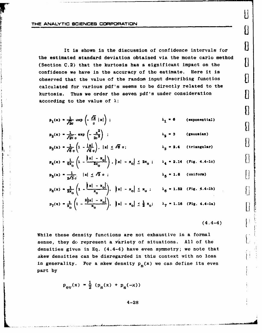
THE ANALYTIC SCIENCES CORPORATION
It is shown in the discussion of confidence intervals for
the estimated standard deviation obtained via the monte carlo method
(Section C.2) that the kurtosis has a significant impact on the [1confidence we have in the accuracy of the estimate. Here it is
observed that the value of the random input describing function
calculated for various pdf's seems to be directly related to the
kurtosis. Thus we order the seven pdf's under consideration
according to the value of A:
11VIL(X) a 0 li)* (exponential)
p2 (x) - A- -3 (gaucalan)
t P(x) " ( 1 ( •i .) - 3 -2.4 (triangular)
1 1 ) - 2x ; A4 " 2.14 (Fig. 4.4-io)
P ) I - I A5 - 1. (uniform)11 -
P6(x) " 21 0 A 1.52 (Fig. 4.4-1b)
a 0
-A -21111-x 0 ; - -X ~4x; A 1.16 (Fig. 4.4-la)
(4.4-4)
While these density functions are not exhaustive in a formalsense, they dc? represent a variety of situations. All of the
densities given in Eq. (4.4-4) have even symmetry; we note that
skew densities can be disregarded in this context with no loss
in generality. For a skew density ps(x) we can define its even
part byF\
Pev(x) = 1 (Ps(X) + ps(-x))
4-28

ITHE ANALYTIC SCIENCES CORPORATION
5 Since the three nonlinearities considered are symmetric (odd) and
the moan values of their inputs are zero, only the even part of5the pdf contributes to the describing function calculation.
Limiter - The ideal limiter or saturation operator,
| ~x , xl ~)" 44
3f(x) 1 sign (x) , Ixi > 6 (4.4-5)
is a common piecewise-linear function used to model nonlinear
phenomena. In Fig. 4.4-2, we portray the various describing func-
tion gains for this nonlinearity, corresponding to the pdf t s de-fined in Eq. (4.4-4), as functions of the ratio of the input rms
level, a, to the saturation point, 6. As would be expected, all
seven quasi-linear gains capture the fact that the effective gain
starts to decrease from unity whenever a significant portion of
the assumed input pdf lies beyond the saturation point, i.e.,
whenever there is a significant probability that lxi is greater
than S. As has been pointed out previously, this effect is thekey to the success of quasi-linearization techniques in reflect-
ing nonlinear system behavior that is beyond the scope of small-
signal (Taylor series) linearization.
It is interesting to observe that the relative positionsof the curves in Fig. 4.4-2 exhibit a monotonic relation to the
value of X. The greater the difference between X for a particu-
lar pdf and the value for the gaussian case (X = 3), the greater
the difference between that density function's ridf curve and the
curve for a gaussian distribution. This behavior holds in all the
cases considered here, and is indicative of the fact that the valueof X is one quantitative measure of how "close" the density func-
tion is to being gaussian. The variation of the ridf's with X is
about at its maximum (on a percentage basis) for the case a 26;
the ridf decreases 13% as X increases from 3 to 6, and increases
28% as X decreases from 3 to 1.16.
4-29

THE ANALYTIC SCIENCES CORPORATION
SIMALL SIGNAL LINEARIZAItON
. • LIMITIR
"UNIFORM ,,ijk
0.4 pTIN L
0 0. 1.0 1.6 o0 2. 30 31 4,0
RATIO OF INPUT STANOARO OIVIATION TO SATURATION POINT. a/&
Figure 4.4-2 Random Input Describing Function VSensitivity for the Limiter
__Pk _ Laww- A similar study was performed for a power-
law characte 'stic,
f(x) = x sign (x) (4.4-6)
This type of nonlinearity is often used to model effects such as
the "hard spri,._' characteristic (Ref. 15) discussed in consider-
ing nonlinear restoring torques acting on the missile seeker head,
Section 3.6. For the power law, the ridf's calculated for the
same density func.tions considered previously have the form (Ref.4)
ni = "ia (4.4-7)
where a is the input rms level and p are coefficients determined
by the input pdf's, pi(x). Thus the describing function gain for
f(x) increases linearly with the input rms level, in direct con-
trast to the small-signal linear gain which is identically equal
4-30

THE ANALYTIC SCIENCES CORPORATION
0to zero, as shown in Fig. 4.4-3. It is again observed that there
is a monotonic relation between Xi and the ridf curves. In this
0 case, an increase in X leads to an increase in the describing
function gain, which is contrary to the behavior shown for the
limiter. This is a result of the fact that the power law output
increases more rapidly with increasing input than a linear charac-
teristic, whereas the opposite is true for saturation. For the
power law nonlinearity, the ridf sensitivity is independent of a,
i.e., the ratio of ridf's calculated foir pj(x) and pjfx) is simply
1i/3j. For f(x) in Eq. (4.4-6), the describing function gain n
varies from + 33% for the exponentially distributed case, to -34%
for the pdf P 7 (x", compared to the gaussian input ridf, whichshows that this nonlinearity is somewhat more sensitive to vari-
[1ations in X than the limiter.
C ms
POWER LAW NONLINEARITY EXPONENTIAL
~2.0
GAUSSIAN
is TRIANGULAR/000ý_P4
UNIFORM
PC
-!5
'•' [ • SMALL SIGNAL LINEARIZATION
I0
0 0.2 0.4 0.6 0.8 1.0 1.2INPUT STANDARD DEVIATION, a
Figure 4.4-3 Random Input Describing FunctionSensitivity for the Power LawNonlinearity
4-31

tATHE ANALYTIC SCIENCEB CORPORATION
Sinusoidal Operator - The third nonlinearity considered [1i n thevsv svns it. lvi t.y studivs Is th, I.h, si n ida I.r I opraitor,
f(x) - sin x
which is needed to resolve the missile and target velocity vec-tors in the missile-target intercept model, for example. A po- ttential source of difficulty with this function is that the non-
linearity output periodically changes sign with increasing or IIdecreasing values of its input. This leads to quasi-linear gains
that, for large values of rms input, u, may even differ in signfor different input pdf's. This problem is not unique to CADET;in many modeling and simulation studies, care must be exercised
when the input to a sinusoidal operator (or any other trigono-
metric nonlinearity) can exceed ± 90 deg (t n/2 rad), since insome sense the "gain" can change sign in some situations. Bear-
ing this in mind, we have calculated the random input describing
functions for values of a as large as 3 rad to indicate where
such effects become important, as shown in Fig. 4.4-4.
The quasi-linear gains for a < n/2 rad show some simi-larily to those obtained for the limiter; this is a reasonable
mode of behavior, since the sine function shows a definite satu-ration effect of the range lxi K ir/2 rad. As expected, the ridf's
are inversely related to X for u < Tr/2 rad, i.e., as X increases,n decreases. However, as the input rms level approaches 3 rad,
the describing functions for all of the pdf's except pl(x) andP2 (x) become negative, and the monotonic relationship between X
and n appears to be lost.
The preceding studies 4ndicate that the sensitivity of
random input describing fune-t.ion calculations to variations ininput probability density function is slight for small values of
input rms level; as a approaches zero, the quasi-linear gainsapproach unity for the limiter and sinusoidal operator, and zero
4-32
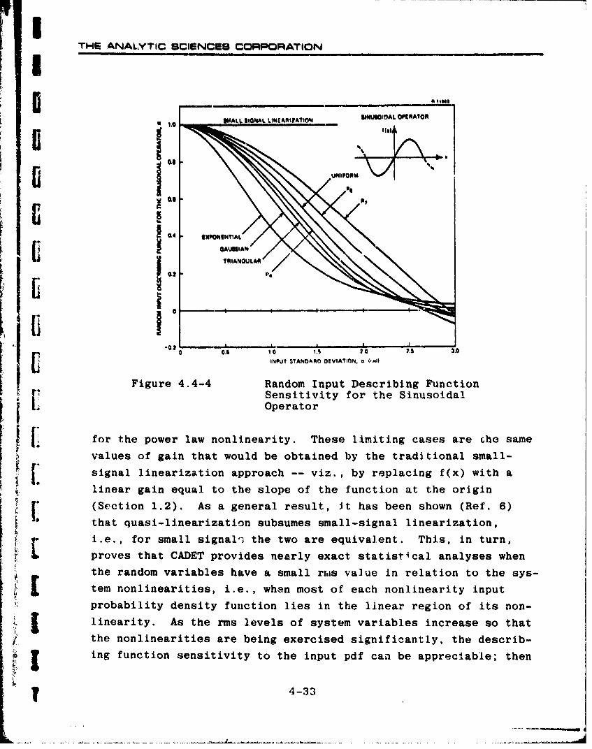
THE ANALYTIC SCIENCES CORPORATION
SII
g - p g w
ALL SIGNAL LINEARIZATION SINUSOIDAL r h OeRAn
Ikrth oer 0aolnaiy Teelmtn assaetesm
~~ 04 OIVO4NTIAL
-0.1 ! 13 2 *21*50
INPUT STANDARD OEVIATION. U 0,101
Figure 4.4-4 Random Input Describing Function~ Sensitivity for the Sinusoidal
L Operator
[ [ for the power law nonlinearity. These limiting cases are che samevalues of gain that would be obtained by the traditional small-
signal linearization approach -- viz., by replacing f(x) with a
linear gain equal to the slope of the function at the origin
(Section 1.2). As a general result, Jt has been shown (Ref. 6)
that quasi-linearization subsumes small-signal linearization,
i.e., for small signal.• the two are equivalent. This, in turn,
proves that CADET provides nearly exact statistical analyses when
the random variables have a small rrms value in relation to the sys-
tem nonlinearities, i.e., when most of each nonlinearity input
probability density function lies in the linear region of its non-
linearity. As the rms levels of system variables increase so that
the nonlinearities are being exercised significantly, the describ-
ing function sensitivity to the input pdf can be appreciable; then
T 4-33

THE ANALYTIC SCIENCES CORFPORATION
it must be ascertained how sensitive the system performance is to
variations in gain at each point in the system model where a non- 11linearity occurs. No general answer can be given to this question;
the verification of CADET for particular applications must be 13accomplished by direct comparison with monte carlo results, as has
been done in Chapter 4 of Ref. 4 for the missile homing guidance
system.
4.5 DESCRIBING FUNCTIONS NOT EXISTING IN CLOSEDFORM UNDER THE GAUSSIAN ASSUMPTION
For certain nonlinearities, random input describing func-
tions cannot be obtained in closed form under the assumption that
the inputs are jointly normal. In this section we indicate some
approximate methods for computing ridf's that involve either ap-
proximations to the input probability density function, or approxi-
mations to the nonlinearity, and discuss their usefulness.
An example of interest in the missile-target intercept
problem is the nonlinearity
f(xy) - (4.5-1)
which defines the missile-to-target range in terms of the cartesian
components of the separation, x and y. This problem is considered
in some detail to provide a focus for the discussion of several
ridf approximation techniques. We compare the accuracy of each
approach for the nonlinearity given in Eq. (4.5-1), and point out
some pitfalls that may be encountered if care is not taken.
In order to simplify the discussion, we assume that y
does not have a mean component, and x has a negligible random
component. This approximation is valid in many missile-target
intercept situations except at the very end of the engagement
(refer to Section 4.1 of Ref. 4). With these assumptions, there
4-34
mTHE ANALYTIC SCIENCEB CORPORATION
are only two ridf's, f and ny, needed for a quasi-linear repro-
sentation of the range. Thus from Eq. (4.1-), we seek to evaluate
f x [A Ti' * p.(y)/' y- dy
n yp(y) /-:y
l Under the assumption that y is a gaussian random variable, the
second of these integrals can be evaluated analytically; however,
the first, which is of the form
A~ 11m 0 2f a /smx + y 2e L ]~ dy (4.5-2)
w•y
C cannot generally be solved in closed form unless mx - 0, in which
case we have
f =EEIyI /2;WO'a (4.5-3)S~y
For the more general situation given by Eq. (4.5-2) with mf 0,!it is desirable to use some approximate technique to obtain a
I. closed form expression for f that is convenient for use in a CADET
r analysis.*
A Taylor series expansion of a function of a random vari-
able, f(y), about the mean of that variable, m, results in
Idf r + .1 d I 2÷ 2+ <•f(y) f f(m) + r -f). y-m
dy-Mr 2 df - mj r+... (4.5-4
While f in Eq. (4.5-2) fr given values of mx and oy can be cal-culated by numerical integration, a less time-consuming approachis desired for repeated evaluation in a CADET analysis.
........m

THE ANALYTIC SCIENCES CORqPORATION
where r y-m. We desire to determine the expcte.('d value of the
abov, function, which is given by
Ic~ 2 +d 3 fl I!Ef(y)] f(m) + 1--:-•l- y-m ] +
(4.5-5)
where use is made of the fact that E Cr] is zero to eliminute
the second term in Eq. (4.5-4); all other odd central moment
terms (E Er 3 . etc.) are also zero for symmetric pdf's. Truncat- .
ing the series given in Eq. (4.5-5) at the second term, we obtain
S1 d 2f 2L
E [f(y)]~ f(m) 1 d 2 2T (4.5-6)d y
which is an approximation suggested in Ref. 8. We note that this
result is independent of the particular density function of y. Ifmore terms are desired, the higher-order central moments can be
evaluated using a specified pdf. If y is gaussian, all odd cen-
tral moments are zero and even central moments are given by
(Re 1. 8)
2kja Ik~11 2k E [r"' (1 ((3) (5). . .(2k - 2
as can be inferred from Eq. (4.3-6). Thus the full expansion is
E Ef(y)- f(m) + 1 d 2 fj 2 + (1)(3)2 d4 fl 4+2 2?Y 4! d 4I m (157
E E~y• "f~)+ y Y =--, M dy4 Y'"
(4.5-7)
The use of the first term alone in Eq. (4.5-7) corres-
ponds to small signal linearization; taking two terms as indicated
in Eq. (4.5-6) results in a quasi-linear gain that is often use-
ful. We observe that the existence of a well-behaved (i.e.,
4-36
THE ANAL'Y'TIC SCIENCES CORPORATIONI! convergent) expansion for f(y) does not guarantee that Eq. (4.5-7)
exhibits the same behavior.
In the present case, the series expansion approach is
* effective for evaluating f only in situations where mx is con-
siderably larger in magnitude than ay, due to the singularities
of the derivatives of /m2 at the origin (mx = 0). To demon-
strate this difficulty, we write the series expansion for the
nonlinearity under consideration (Ref. 19),
f(y) = +//; -Y7 Im2l (4.5-8)tX X r x 2" m - 8 X) + . . 4 5 8
from which we obtain
' f lmxlI I + ½1 (ay rx
_ Z + (4.5-9)
as an approximate describing function to represent the mean com-
ponent of the range. For mx considerably larger than uy, the
first few terms of this expansion yield acceptable accuracy.*
I. IHowever, since mx approaches zero as range goes to zero in the
missile-target intercept problem, using Eq. (4.5-9) is generally
not suitable.
r TA second method for approximating the integral in Eq.
(4.5-2) is the substitution of a nongaussian pdf for which the
integral can be obtained in closed form. As in previous sensi-
tivity studies (Section 4.4), the best result is obtained using
the triangular pdf. Substituting this distribution into
K We note that the expansion indicated in Eq. (4.5-9) never con-verges formally, i.e., for any value of ay/mx, no matter howsmall, the series will eventually diverge as more terms areevaluated. This is a standard property of asymptotic expansionswhich are useful only when truncated after a finite number of terms.
43

71'THE ANALYTIC SCIENCES CORPORATION
Equation (4.5-1) leads to an integral that is evaluated in closed
form to be
f m+V log + (3(1+V2)/)]Lf x 1+v 2+2)
(4.5-10)
where the auxiliary variable v is given by Vm
v - (4.5-11)ray
The accuracy of Eq. (4.5-10) is quite good, especially when com-
pared with the poor approximation given by the series expansionin Eq. (4.5-9) when ImxI is less than or equal to ay. The error
ybetween Eq. (4.5-10) and the exact result specified 'n Eq. (4.5-2),as shown in Fig. 4.5-1, is less than 3%, which is adequate for. ,!
most applications.
We note that the conclusion that the series expansiontechnique is not useful for computing the ridf in the case treated
above should not be taken as universally true. When series ap-proximations for an ridf can be obtained which are accurate overthe entire range of the input statistics, they will generally f}yield good results. Another important consideration is that theseries expansion technique is generally feasible for highly nom-plicated nonlinearities, as demonstrated in Section A.4, while
evaluating f by integration with any approximate pdf p(y) may beimpractical or impossible. The cases treated in Section A.4 thusillustrate the power of the series expansion technique, given inEqs. (4.5-6) and (4.5-7), while the above presentation indicates
the care that must be exercised to avoid convergence problems.
This chapter presents a detailed outline of the theoryand application of statistical linearization. Guidance in
4-38

THE ANALYTIC SCIENCES CORPORATION
STAYLOR SERIES EXPANSION
U.
z
F@LU TRIANGULAR
~~~ DENSITIY ENIT
"F 1
WN
< EXACT SOLUTION,0 GAUSSIAN DENSITY
zI•0 I I , , ,
0 0.5 1.0 1.5 2.0
NORMALIZED MEAN VALUE OF DOWNRANGE SEPARATION, mx/ay
Figure 4.5-1 Comparison of Approximations for
the Expected Value of the Range
deriving random input describing functions is supplled in a
variety of examples, and a comprehensive discussion of the sen-; .sitivity of ridf calculation to deviations from the assumption
of joint normality is provided. These contributions should aid- future users of CADET in performing statistical analyses of non-
linear systems with random inputs, and in assessing the accuracy
of their results.
I
T 4-39

53.1 DIftiCT CAflBT-MOT CARLO COMPARI3QSI
S.uce CADET and the monte carlo method are tba Obly tools
available for the statistical analysis of the perform~ce of nsa-
U linear system with random inputs, tho ultimate value of C6T coz
only be established by comparing the relative efficacy of the tv.)approachea. In ibis section, we will touch on utilit., o
Spplicatio e udure ocomuter e, and our Baegon these factors, znd on other characteristicm if the two tech.
Sniques, we will outline the philosophy for th. a,,-pli1cmtion of MADETthat has been developed at TASC, and summarize the strong and wo"points of this methodology. The conclusions, while bgwed chiefly
on extensive experience gained in treating the missile-target
tiin-'pp pr.hi-a , a 1,4l pro4da us. _L gu4ila o rae
W •applications of CADET.
A5.1.1 Overview and CADET Mechanization
In Chapter 1 we have derived differential equatious gov-
[erning the approximate evolution of the mean vector and covwr ance
matrix of non]inear time-varying systems with random inputs, Lav-
ing the form
. f (L,,t) + G _;) w(t)
Swhere x(t) and w(t) are vectorFý comp<ssd of the system states gid
random inputs, respectively. (Refer to Section 1,2 for further
details.) Btifore the CADET equations can bc iatplemeated, it is
necessary to have the random input describing functions (ritfds)
required for a quasi-Linear representation of every system
5-1
-- - - -,A- -. - - - * ---r- ~ ~ --- ~-

THE, ANALYTIC SCIENCES CAPOSRATION
nonlinearity. The ridf's for a broad set of single-input non- 4linearities are directly available from Ref. 6 (see also Appen-
dix A). In addition, Chapter 4 of this handbook providss ridf's 7)
for a number of common multiple-input nonlinearity formt Con-
sequeatly, use of CADET is often a matter of direct substitution
of knrt.n ridf's in the mean and covariance equations, as demon-
strated iur Chapter 2. If a matrix computer language is available
to the analyst, the construction of a computer program for apply-
ing CADET is no more difficult than the programming required for
using the monte carlo method. As an added benefit, CADET does
not necessitate use of a raqdom number generator; a common source
of concern in the monte carlo method is the question of what con-
stitutes a "good" random number sequence and how such a sequence
can be generated.
Thus from the point of view of utility and mechaniza-
tion, the two techniques appear to be quite comparable -- there
is no clear-cut reason to state that one technique is superior
to the other based on these considerations.
5.1.2 Accuracy and Efficiency
One of the main arguments that can be advanced for the
use of CADET in obtaining projectiois of nonlinear system per-
formance is the significant reduction in computer central pro-
cessing unit (CPU) time achieved by using CADET instead of the
monte carlo method. In making this comparison, two issues must
be addressed: the number of monte carlo trials that must be per-
formed in order to obtai comparably accurate results, ant the
practical limitation imposed by computer costs. From the stand--
point of accuracy, a decision regarding the required number of
monte carlo trials is somewhat arbitrary, because the error
mechanisms of CADET and the monte carlo method are dissimilar.
5--
i • Referring to Fig. C.3-2b, we note that, in a situation where the
statistics are quite nongaussian, the CADET computation of the
rmms value of a system variable appears to be at least as accurate
as the value estimated with 400 monte carlo trials, in the sense
L.. that the 95% confidence band for 400 trials brackets the CADET re-
sult. Where the statistics are more nearly gaussian, e.g. as in
Fig. C.3-2a, it would seem that CADET accuracy is comparable to
Ii |•"that achicved by more than 50C monte carlo trials.* On the other
hand, a pragmatic evaluation of the efficiency of CADET should take
E: |in.o account the fact that most monte carlo studies must be limited
in scope by computer budget constraints. A reasonable upper bound
[ fis thusv 256 trials since, in the gaussian case, this results in
93% confidence that an accuracy of 10% can be achieved (Section ?.2);
r f'or high-order systems, even this number of trials may require an
It.nordinate amount of computer time. For the present discussion,
we therefore compare the relative efficiency of the monte carlo
L and CADET approaches on the basis of 256 trials, recognizing that
the estimated -ms values of the system variables obtained for this
Snumber of mo-nte carlo experiments may be Less aceurate than theLCADET results.
In piist studies, Refs. 1 to 4, the savings in computer
CPU time achieved by the application of CADET has always been
[ significant in comparison with 256-trial monte carlo studies, even
though the system treated in &:ome cases has been of high order
(with up to 42 system states) and very nonlinear (having up to
26 nonlinearities). We discuss below how both of these factors
tend to reduce the relative fficiency of CADET.
Monte carlo simulation for a system with n states requires
the integration of an n-vector differential equation (repeated q
times where q is the number of tr!.als), while CADET involve& the
Recall that CADET is exact in the linear gaussian case,Section 1.1.
Ii 5-3' j

THE ANALYTIC WIENC*S C=PUPORATIC)N
propagation of the n-element mean vector, m, and the nxn symmetric
covariance matrix, P -- a total of n(n+3)/2 elements. Thus the2computational burden for CADET can increase as fast as n /2 while
the CPU time for monte ct~rlo analysis only varies as n, demonstrat-
ing that an increase in the number of states may reduce the ad-
vantage of CADET in efficiency. This factor can be mitigated to a
large extent when there is little dynamic cross-coupling in the
system; in the quasi-linear system model, Eq. (4.1-4), this cor-
responds to N having few non-zero elements (N being sparse). In
many practical problems, N is sparse and a considerable increase ")
in the computational efficiency of CADET can be realized by the
application of techniques which circumvent multiplications in-
volving zero elements, thus streamlining the evaluation of p .1
(Eq. (1.2-7)). Such an approach has proven to be valuable in the
studies presented in Ref. 3.
The number of nonlinearities may also increase the com- "
putation time required by CADET, since the calculation of a ran--
4 A~a%.4 XUU fultu L-- 7 nLI requuires mor iowicai and
numerical operations than evaluating the corresponding nonlinear
function in the monte carlo program (refer to Appendix A, for
example). The investigation treated in Ref. 4 was exceptional in
having nearly as many nonlinearities as state variables; more
typical applications of CADET would focus on a few principal non-
linear uffects, leading to a still more favorable comparison of
CADET with the monte carlo method in terms of computatioi it burden
per performance evaluation.
Using the •same integration method in performing the monte
carlo ensemble of simulations as was used in prcpagating the sys-
ter mean vector a: d ecvariance matrix via CA)ET, and assuming that
the same integration step size is required in each procedure, the
results summarized in Table 5.1-1 indicate the effect of the sys-
tem dimensionality (number of states) and degree of nonlinearity
(number of nonlinearitiee) in typical studies of the mi.ssile-target
,5-4

TA3LE 5.1-1
COWMARISOI OF CADET AND MONTF CARLO EI"CIENCYI BASED ON 266-TRIAL MONTE CARLO ANALYSIS
Nast" Number of Ratio of Computer Time Costs.,
of 8tateu*n oalinearitl* Monte Carlo/CADXT
R V2 1 30
Rot. 3 17 5 15-20
Rief. 4 22 22 10
23. 42 26 20-30**
*Coatinuous- ano discrete-tims dynamic states ')nly; biasS[7 states 06ittod.
Optimized, usiag fast sparse-matrix-mltiplication
intercept problem. Ccpwaring the InvestfiitinnR od' Ref• R 2 and 4, I
I ..• we note a considerable decrease in relative CADET efficiency caused
by increased s-' 3mp ity; in the analysis of the system
model given in '. 3, an intermediate degree of complexity and
corresponding efxiciency is noted. The study of Ref. 23, also
indicated in Table 5.1-1, shows the significant iwprovement that
can be achieved by careful CADET program optimization, using the
fast sparse-matrix.-multiplioat ion subroutine approach mentioned
above.
[ We should also point out that in some circumstances the
monte carlo approach may require a reduced integration step size
to avoid failure of the numerice" '-tegration technique (refer to
Section 4.4 of Ref. 4, for examr .. In such cases the monte
Id[ carlo/CADET CPU time ratio will be even higher,
r5-L Ii
5.2 OTHER FACTORS AND PRILOSW OF APPLICATION
In comparing GAUST and the monte cario uethod for use ix
obtaining performsace project'ons for nonlinear systeam witb rma-
dom iuputs, we have observed that there are several significant
similarities. Both techniques are applicable to nonlinear sys-
tem models with an arbitrary number of states and nonlinearities,
and we often rely on the gausslan assumption in enosseing tie
accuracy of the performance statistics obtained (refer to Sec-
tions 1.2 and C.2). In either case, departure from normalL1y
can be compensated for to a certain extent; in CADW?, nongaussian
probability density functions can be used in calculating de-
scribing functions, while in monte carlo simulation the fact that
the confidence band linits may increase for nongaussian random vari.
ables (Fig. C.2-2) can be counteracted by increasing the number
of trials performed. The princilpe trade-off between the two
methods is in elfic:Leucy versus versatililt.
statc, trajectories (Eq. (C.1-4)) can be used not only as a data
base for calculating estimated performance statistics m"() and
P(t) at instant-s of time of interest, but also for estiamting
highe- order moments, and for generating histograms whiLcb are ap-
roximate density functions for the variables undmr considera-
tion. however, -he versatility of the monte carlo method can only
be exploited with a further tgnificant increase in computer time
expenditure over that indicated in Table 5.1-"; while the esti-
wation of ni and P may require several hundred trials or mire, it
is generally necessary to perform thousands ef trials in order to
obtain an accurate estimate of the pdf of a random variable (and,
cf course, what constitutes an "accurate estimate" is generally a
subjective value judgment in a nongaussian case). In the sense
that one can always obtain a, better estimate of the statistics
of a rardom vaitable by running more trials (compýter budget per-
DJ~tting), t!,e monte carlo method is a "self-checking" procedure.
5-_6-E

THE ANALYTIC SCIENCES CCWW T"1OAT1N
, •CADRT, on the other hand, provides approximate valuea for m(t)
and P(t) in a single numerical integration of the quasi-linear
covartance equations (Eq. (1.2-7)), usually in a small fraction
K of the computer processing time required for an accurate monte
carlo analysis.
One of the primary purposes of the statistical analysisr of nonlinear system performance is the evaluation of the change in
system effectiveness due to variations in random input levels,
initial condition statistics, system parameter values and second-
ary nonlinear effects. The multiplicity of factors such as these
implies that the analysis will generally be C )ne repeatedly, and
computational efficiency is thus an important consideration. This
point is a strong argument in favor of CADET. On the other hand,
the versatility of monte carlo simulation (with its self-check
capability) permits us to assess the accuracy of the monte carlo
analysis. This is a feature lacking in CADET which makes it
advisable to utilize monte carlo simulation in a monitoring capa-
city, since it is always possible to obtain reasonably accurate
performance projections by increasing the number of trials suffi-
ciently.
I. The effective use of CADET and monte carlo analysis in
concert can be demonstrated in a hypothetical trade-off study wheretwo parameters, say a, and a are to be varied over ertain ranges
to obtain optimal performance in some sense (to minimize rms
1. terminal miss distance in the missile-target intercept problem, for
example). As shown in Fig. 5.2-1, a few points in the parameter
[ plane are chosen for careful CADET-monte carlo comparison (verifi-
cation of CADET); then extensive performance curves are generated
using CADET, from which the optimal values of and a2 are chosen.
If desired, the vicinity of the pctnt of optimality can be studieC
Susing a few selected values of aI and a 2 and performing the required
mo~te carlo simulations. Similar i~pprov.ches can be used in study-
ing sensitivity to nonlinear and random effects.
5-7

Iwo T"0MINAL M$S DWANCI
b POINT OF
Figure 5.2-1 Illustration zaf CADST and Monte CarloAnalysis in a Parameter Trade-Off Study
The overptl philosophy of CADET usagei, based on the atri
I '/ prcdr s/ nrklud
points of both- CA IuT and monte caflo simulation, is illustratedFig. 5.2-2. The initial verification procedure is generally undf
taken for the "nominal systom," i.e., for the gaystem with nomtna'
parameter values, and is of necessity quite meticulous, Thus
several hundred monte carlo trials .aay be performed, and if theri
is reason to believe that the system is highly nonlinear -- so
that the system variables may be quite nongausstan -,- it may be
necessary to investigate higher order moments or histograoms to
decide whether more trials are needed in order to obtain a re-
liable statistical analysis. Once this phase has been complete&,
satisfactorily, the CADET parameter sensitivity studies can then
be performed. Observe that the preliminary careful but time-
consuming monte carlo study is always required if accurate per-
formance statist.cs are to be obtained from monte carlo simulatic
5-8

r .- -- -- ---. ,
THE ANALYTIC SCHENC*SS CC RATION
5 cr :rSENITVTY.STU DIE001
- •v~• WI- -A EAONTVI CURO VNe. CAMN
I I
CAALO 1I0NAft PERFORAMEXNS
7-
F"AO OFPRFR E1NSV
with high confidence. The use of these• statistics to verifyU CADET paves the way for efficiently performing a wide variety ofsen~itivity studies. In the latter analyses, it may be advisable
I" to make comp~arisons with monte carlo results in selected cases to
reverify CADET accuracy. This approach mirrors that used in the
"[ studies described in Refs. 1 to 4.
" 5.3 CAL)ET DEVELOPMENT TO DATE: SUMMARY AND CONCIUSIONS
5-3.111 SESIIVTYSTDIS
A major goal of the studies described in Refs. 1 to 4[ was to extend tbe proven c~apability of thc C ovartancc, Anaiys.•sDEcribiWg Function Technique -- CADET -- to provide accurTte
Ti-r 5.-5,--3ohy 1-MLLfyi~~~v
LA.
[ ... ... .... ... ....... ..
CAETae h a o fiinl efrigawdvreyo

performance projectionr for tactical mtsalle guidance system
models that are quite realist'c -- i.e., that incorporate a nuam-
ber of significant nonlninar anA random effects. The approach
used to achieve this objective has entailed
9 Verification of CALDrr performance projectionsby the use of selected montc carlo perform-ance studies
o Investigation of the sensitivity of CADETanalysis to deviat.ion from the assumption thatthe state variables are jointly normal.
In these investigations, the following effects were treated:
Sources of Nonlinearity
a Guidance law
o Acceleration command limiting
o Aerodynamic effects (nonlinear airframe)
* Missile-target intercept geometry
o Range-dependent seeker noise sources
o Receiver/signal processing characteristics
* Seeker radome aberratione Seeker mass imbalance
# Seeker gimbal Coulomb friction I* Seeker head restoring torques (n',nlinear
spring effects)
Random Effects
* Tracking sensor noise and measurement errors
o Range rate measurement error
*Target maneuvers
*Deviation of initial conditions firoinominal values
Two aspects of the sensitivity probiem, hnve been considered
in Chap',er 4: the Penoitivity of random input descrit-ing func,ýiom
5-10

'rb-s ANALN'Tir, SCWnNCES CORPO:RATION
5 calculations Lo tiLe probability density function of ! he nonl inearity
inpuit, and the calculation of approximate random input dosecrbing
funclions when It is inconvonAent to use the oxact. rosuI t for the
gauesian case.
5.3.2 Conclusions
aThe investigations describod in Refs, 1 to 4 have indeed•• shown tnat CADET 14. an accurate and efficient tool for condu!ýtini
stat ist:ica):_±nae.jve th er fmance of a tactical misleI- ~s_.tstm ,ncludi_.U tLhe el"ffcts of a niunber of significant nonlinear,
1.~a~nd random _phenomTena. T(he• •o,.l--ions drawn, from these studies
can he suilnmrized as foullows:
* L CADET has the demonstrated abA.Lity to capture
tho aiapact of a.ll. of the nonlinear of ectsSlisted above on gitidaitce system perfoimance.
I * lix all cases stud'.ed, CADET results are closeto or within the 95'9, confidenc+. ilmit.s of themonte cario an-.lvf. s for up to 500 trials..LTi s d"Kree or' L it • jt w . 0i I. n1ra.3 y aL ln--t:rined even in the numerous -inst.ances where the
- nonlineo•rtiees werLe sihowa to have a marked
delett-rlous effect on rirs miss distance.
* Even in cases where ',he number of system statesa'd nonlinearities is large, CADET showssignificant computacional advantago over theno)nte carlo method: Between 10 and 30 CADET per-fo'marce proje.,,tions Anve been ottained for thesame ain,:)unc of computler time required by oneaccurate monte carlo study.
* There are certain highly nonlinear cases inwhich C,•DET anasly:is may be inadequate. Typic-ally, theFe are s:tuatotion in which a non-linearity input is unc'orrelated with its output;for a more compi.ete discussion , refer to Sea-tion 4.2 and Appendix B. The Modified CADETmethodology presa-nte.-l in Appendix B appears tooffer A solution to flits problem.
1 fl--ll
rF.Tn-VE ANALYTIC SC3ENCES C7RFNRATION
* Highly nougaussian system variablea not onlylead to inaccuracy in the CADET analysis, butalso make the monte carlo method less reliableand reduce the meaningfulness of the basicstatistical measures of system performance, themean vector and covariance matrix.
a The value of the kurtosis, X, (the fourth cen-tral moment of a density function divided bythe variance squared) is a useful measure ofthe departure of the Jensity of a random vari-able from the gaussian case It would thus bevaluable to estimate this parameter for eachnonlinearity input in the monte carlo analysis Tfto help in appraising the accuracy of the montecarlo method and CADET.
In light of these and related Findings, it is felt that
confidence in the ability of CADET toroivide accurate statistical
analyses of .omplex nonlinear missile guidance systems with a
number of .Landom disturbances has been ouite well established.
Based on the diversity and complexity of the effects studied so
far, it seems reasonable to anticipate that similar results willbe ootai~ned 4.n- applying CADET to a broad spectrum of problems
modeled by nonlinear systems with random inputs. It is hoped
that this handbook will facilitate the further extension of the -
usefulness of CADET, as well as permitting the direct applicatior, Aof the technique to the missile-target intercept problem.
-4
5-12
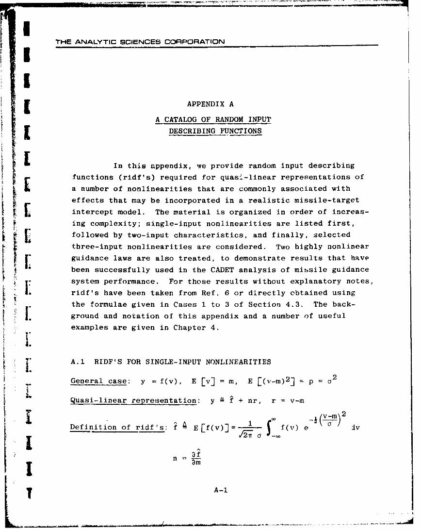
ITHE ANALYTIC SCIENCES CORPORATION
I
'I APPENDIX A
A CATALOG OF RANDOM INPUT
DESCRIBING FUNCTIONS
In this appendix, we provide random input describing
r functions (ridf's) required for quasi-linear representations of
El a number of nonlinearities that are commonly associated with
effects that may be incorporated in a realistic missile-target
intercept model. The material is organized in order of increas-
ing complexity; single-input nonlinearities are listed first,
followed by two-input characteristics, and finally, selected
three-input nonlinearities are considered. Two highly nonlinear
guidance laws are also treated, to demonstrate results that havebeen successfully used in the CADET analysis of missile guidance
system performance. For those results without explanatory notes,
Sridf's have been taken from Ref. 6 or directly obtained using
the formulae given in Cases 1 to 3 of Section 4.3. The back-
ground and notation of this appendix and a number of useful
examples are given in Chapter 4.
A.1 RIDF'S FOR SINGLE-INPUT NONLINEARITIES
General case: y = f(v), E [v] = m, E [(v-m) 2 ] p = a2
Quasi-linear representation: y f + nr, r = v-m
Sf~v) v
Definition of ridf's: f^ E f(v) 1= f(v) e dvA Cv
I nSI am
S T A-I

THE ANALYTIC SCIENCES COPPOFIATION
A.1.1 Simple Analytic Nonlinearities
y = sin(v) jjf e- sin m
(A.1-1)n -e p cos m
y = cos(v) HI-A cos m
(A.1-2)n -e-ip sin m
y =v2
2 Af n, + p
(A.1-3)21
f= m(3p + m2 )
(A.1-4)
n 3(p+m2 )
y =V4
f = m + 6m2 p4- 3p 2 A1
(A. 1-5)
n = 4m(m 2 + 3 p)Ti
y =V5
f, = M5 + 10M p + 15p m
(A.1-6)n = 5m4 +6m2 p + 3p2
Results for higher powers can be obtained directly using the
relations given in Example 4 of Section 4.3.
A-2

ITHE ANALYTIC SCIENCES CORPORATION
A.1.2 Nonlinearities Involving Sign (v) andPiecewise-Linear Characteristics
Nonlinearities in this group require evaluations ofPF(w), PI(w) and G(w) given by
PF(w) = 1e-w
-2e
r[PI(w) = PF(w) dw (A.1-7)
[ SwG(w) - PI(w) dw = wPI(w) + PF(w)
S-(For more details, see Example 3 of Section 4.3.) For convenient
reference, the piecewise-linear gains listed below are depicted
S[in Fig. A.1-1.
BR-16240
y f(v) y f(v)
Ia) Ideal Relay M Ideal Limiter
y f(V) y FMv y f(V)
--- I 182- )
-2 8 -_ ' 2_81 |
0c) Linear Gain With Dsado one (d) Relay With Deadzone to) Limiter With Deadzono
Figure A.1-1 Basic Piecewise-Linear Characteristics
A-3

THE ANALYTIC SCIENCES CORPORATION ii I
Ideal Relay y = sign (v) j
f 2PI - 1 ((A. 1- 8)
=2 PF "F )
Ideal Limiter V, IvI_< '
6 sign(v), Ivf > 6 -7
So(6+m)- 7•]- 1n =PI + PI -1)
Linear Gain 0, ,vI < 6 -6
With Deadzone y = ( vf "
(A.1-10)
n = 2 P(-PIa) -I
Relay With 0v _< -Deadzone 1, IvI > 6
P(6+M-P -P)
(A.1I-1)SF+A-4
n 1 [- pF(-T , + PF ( -
A-4

THE ANALYTIC SCIENCES CORPORATION,I
_o0 , <vi _<6
Limiter WithDeadzone y (Ivl-61) sign(v) , 61 < lvi 62
1(62-61.) sign(v) , +2 < Ivl
f m G(2]o (G~ m (G -tL L -G[-) ( -6:--(6 2+m) 62-r m6-
P1 na )I -- + PI -_ PI -PI\ + /
We observe that ridf's for a large number of more con°-
plicated piecewise-linear characteristics can be obtained by
decomposing them into a linear combination of the basic nonline-
I arities shown in Fig. A.1-1. To cite two examples, a multi-level
ideal symmetric quantizer can be expressed as the sum of several
r • characteristics of the type portrayed in Fig. A.1-ld, and a
change from unity gain to a gain of k at breakpoints L 6 can be
I represented by a linear unity gain plus the characteristic of
Fig. A.1-lc multiplied by (k-i). These procedures are demonstra-
-l ted in Fig. A.1-2. From decompositions of this sort, the asso-ciated ridf's can be obtained from the results given in Eqs.
(A.1-8) to (A.1-12) by simple addition; for the above examples,
we obtain:
Five-level Symmetric Quantizer (Fig. A.1-2a)
p (++-pm + P1 /36+2m+ -P (P6-23PI ---+ -- - 2m •+ P • ' • • ? P - 2m
( +•.o2 -cr• (M)= 2c 2cr+ +n -1PF16+2m +PF /6-2m + PF 36+2m + PF (36-2m
2/2o 2a 2a
(A.1-13)
A-5

THE ANALYTIC SCIENCES CORPORATION
R- 16239
y f(v) f 1 (v) fY(v)
-38/2 -8/2 V-81/2 -38/ FSj ,8/2
(a) Decomposition of a Five-Level Symmetric Quantizer
f, ): v f2 )-,
-s .! I sk+ ..p•,j "
SLOPE'.. Z ---
(b) Decomposition of a Gain-Changing Nonlinearity
Figure A.1-2 Decomposition of Complicated Piecewise-Linear Characteristics into Basic Components
Gain-Changing Nonlinearity (Fig. A.i-2b)
f = m + (k-1) 2m- a G- 6-rn H) G( a
(A.1-14)
n = 1 + (k-i) 2 - Pi(Q--•) -PI('-M)
The functions PF, PI and G (Eq. (A.1-7)) also occur in
quasi-linearizing nonlinearities having the factor sign(v). Three
~nwwti e-x:iniple- of this ty.'pe of characor. -J. Ij,: :y-r.
Absolute Valie Function y v sign(v)
f = 2 o -m 2aG(~ - 1(A. 1-1.5)
n = 2pI()-
A-6

THE ANALYTIC SCIENCES CORPORATION
i Odd Square Law y v 2 sign(v)
I . 2mPF(,) + ,(m2+a2) [2Pi ( _)-j]
(A. 1-16)
[ n 2 4aPF() + 2m [2PI(!!)-1]
Exponential Saturation y 1-es (v)
*a2
m 1n+=e2e [,_r, + -L PF(c nr+a
F A-71
I. These results complete the catalog of ridf's for single-inputA nonlinearities.
A.2 RIDF'S FOR TWO-INPUT NONLINEARITIES
General case: y = f(vl3 v2 ), E Evil] mi, ri vi- mfi
Tj p11 p1 2 1~ PC1a2
L1 UP12 P22 1 [1 2 0 2
Quasi-linear representation: y +_
I A-7
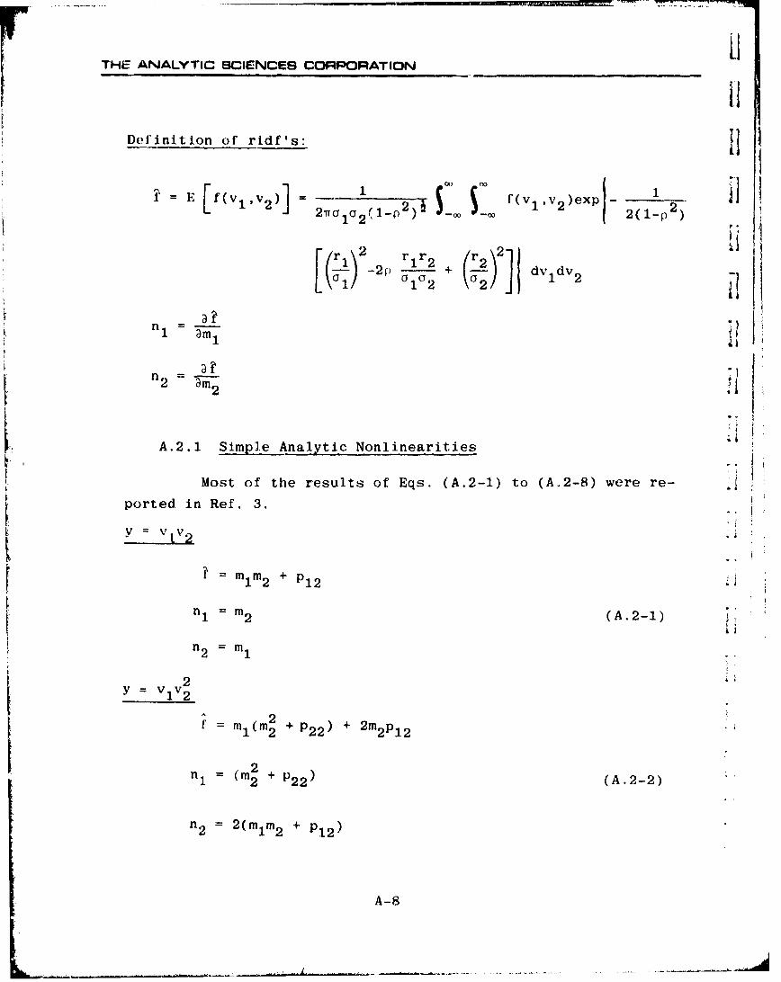
THE ANALYTIC BCIENCES CORPORATION
Definition of ridf'Is:
I' = E f(vl,v 2 )] 2 f(v, v2 )exp _ 1 227t al12(1-p2 ] -= - 2(1-p )
r 2 _ r Ir2 + (r2, 2
2(f) i22] dv dv2
ama
3m2
A.2. 1 Simpl.e Analytic Nonlinearities
Most of the results of Eqs. (A.2-1) to (A.2-8) were re-
ported in Ref. 3.
Lii",y=V LV2
M m
M (A.2-1) "
n2 M1 2n 2 = m1
2y = vlV2
1 2 + P 2 2 ) + 2m2 P 1 2
n (Mi + P2 2 ) (A.2-2)
n = 2(m 1 m2 + P12)
A-8

THE ANALYTIC SCIENCES CORPORATION
I YV 1 V 2 u
_ 2 2f - 3m1 m2 (m 2 +3P 2 2 ) + 3p1 2 (m2 +P2 2 )
2=M 3 (A. 2-3)1 2 (m2 2 2
= 2n2 3m1,(m 2+p 22) + m2pl2
[y VV2
( 2 _( 22+ 2 p+2-(mI pll )(m 2 +p 2 2 ) + 2P 1 2(2mlm2 +P 1 2 )
]n 2ml(m+P 2 2 ) + 4m2 P1 2 (A.2-4)
n 2m 2 + 4
n 2 = 2m2 (m2÷p 1 1 ) + 41iP 1 2
Iiy v I Cos 2 -•P22
ji f e (mi cos m2 -P 1 2 sin i 2 )
Sn =e '22 cos m2 (A.2-5)
22•- -iP22
n = -e (m 1 sin mi2 + P 1 2 cos mi2 )
y v sin v2
f e-4P22(m1 sin m + p1 2 cos m2 )1 -2 22
n= e sin mi2 (A.2-6)
I 2= e&P22 (mI1 cos m 2 - P1 2 sin mi2 )
A-V A-9
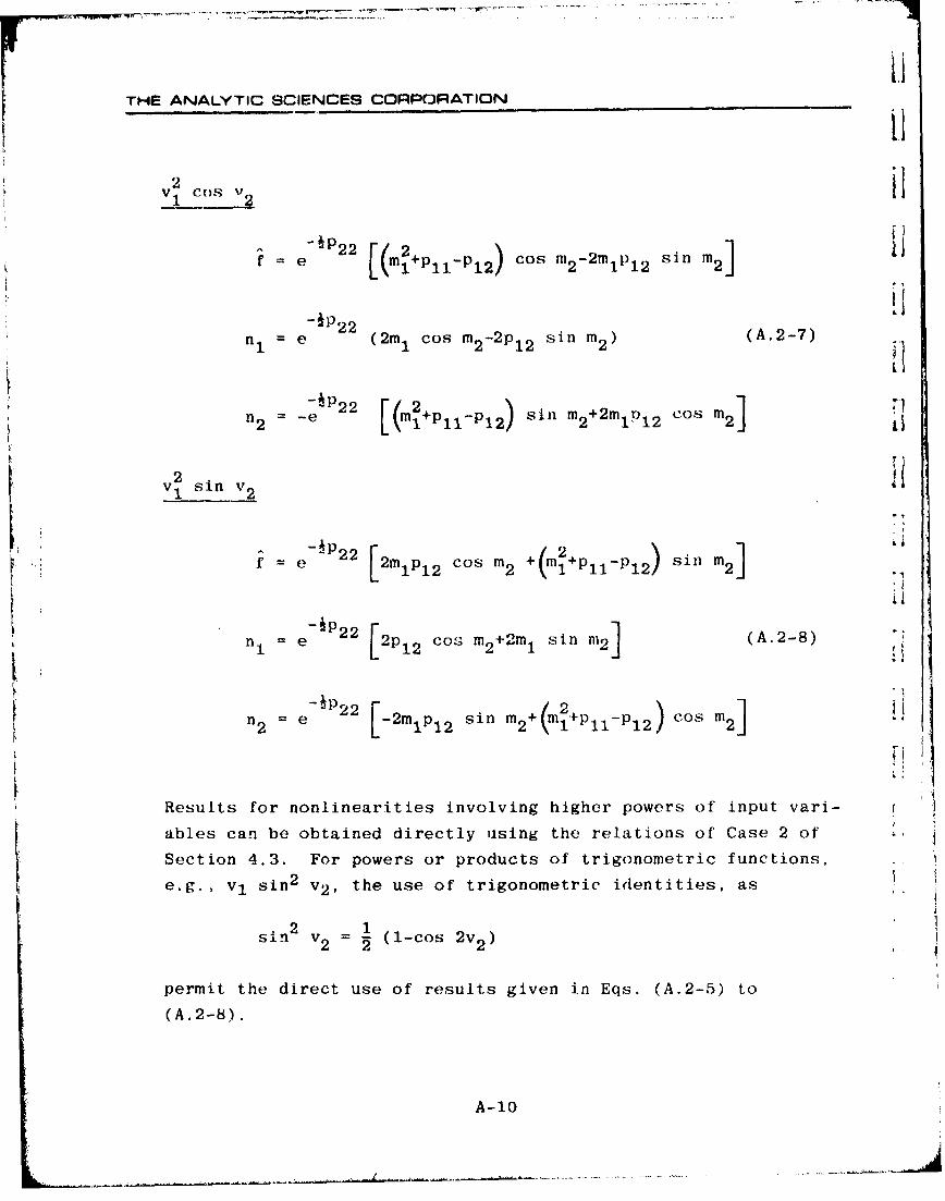
THE ANALYTIC SCIENCES CORPORATION
2 V COS V
e1 2 [( 2) Cos m2-2mIp12 sni 2 ]
n = e (2m 1 cos m2 -2p 1 2 sin In2 ) (A.2-7)
2 e-P 2 2 sin m +2m Cs2
2 -e[(mP11-P12) 12os m2]
v1 sin v 2
fe 2m:P12 Cos m2 + 1+P11-P12) siIn 2]
•, -'P22 ( A.2-8) -SnI = e ~2pl2csm+m sin m2 .
12 con e-'P22 -2mP2 sin m2+ +p -P2Cos m2
1P1 =2(1P1P2 2]-
Results for nonlinearities involving higher powers of input vari-
ables can be obtained directly using the relations of Case 2 of
Section 4.3. For powers or products of trigonometric functions,
e.g., vI sin 2 v 2 , the use of trigonometric identities, as
sin 2 v (1-cos 2v 2 )
permit the direct use of results given in Eqs. (A.2-5) to
(A.2-8).
A-10
IITHE ANALYTIC SCIENCES CORPORATIONI
i [ A.2.2 Analytic Nonlinearities Without Closed-FormGaussian ridf's
j The quasi-linearization of the range,
.7 .. 2
is treated in detail in Section 4.5. Note that it was assumed
1. that x a m x, i.e., the down-range component of the missile-target
separation is essentially deterministic, as is true for head-on
Ji intercepts (Fig. 3.5-1). In this case, the range is a function
of one random variable, y. We further noted that the most effec-
tive approximate ridf for this nonlinearity was obtained by using
the triangular distribution for y (Table C.2-1); this result is
given in Eq. (4.5-10).
In the seeker noise model, Sect±on 3.6-I, related non-
linearities arise in the range-dependent components of the noise.
Thus approximate ridf's for the following two nonlinearities were
obtained in Ref. 4, based on the triangular distribution for y:
Range Proportional Noise y Mv1vx 2
1."~M ml~v I++)•+2 33,2)]
f • -- sign(mx) 1 log + -- + 3
.nI 1 m-• (A.2-9)
n n2 P1 2 [(1+4v2)/j77 -4V+-3V log
where v is an auxiliary parameter given by
I (A.2-10)
A-1i

LITHE ANALYTIC SCIENCES CORPORATION
[IInverse Range ')roportio'nal Noise Y -'x.... 2[
I 2i
f a A• a2 log V + V - lv~
AI
n1 fl (A. 2-11) [
coordinate representation e1 the missile-target separation, viz.[1
n lo +~1 , 2 2 a'(i A -22 v2
The approximate ridf's for this nonlinearity were also derived
inRf 4 sngtetruncated epnintcnqedemonstrated •in Section 4.4, as follows: t
coordinae repre y = mini(vl/V2 )
loin the- tan•/ e expansionl2(P2-technique1 '!
ta = 2 1 2 (A.2-12)
-m1
2 2mt +m2
A-12

THE ANALYTIC SCIENC,.. CORPORATION
IThese results conclude the presentation of ridf's for two-input
nonlinearities.
I A.3 RIDF'S FOR SELECTED THREE-INPUT NONLINEARITIES
I The following results are useful for nonlinear airframe
models as described in Section 3.4; many of these ridf's were
first reported in Ref. 3.
y VlV 2 V3
1 f = m1 m2 m 3 +mP 2 3 +m 2 P 1 3 +m 3 P 1 2
n 1 M 2 m 3+P23
m-n (A.3-1), |,~n2 m mlm + l
I nl3 1mm2 +P 1 2
2v =V 2 V 3
. • 2 (m3+P: 3 3 ) (mlm2 p 1 92)+2m3 (nilP2 3 +rn 13)1 2P3P
-,nI m2 (m2+P 3 3 )+2m 3 P2 3 (A32
.. ~ 2A 3-2
2-. , n2 = m2(m 3 +P 3 3 )+2m 3 P 1 3
n 3 = 2(m 1 m2 +P 1 2 )m 3 +2(m1 P23 +m 2P13)
3y = vv2v3
2"f m = m 3 (m 3 +P 3 3 )(mm 2 +p )+3(m3+p) )(mlp 2 3 +m 2 p 1 3 )+(m 3 P 1 3 p 2 3
n m2 m3 (m3+3p3) +3p,,)(m +p ) (A.3-3)23 -3 3 33
S~A-13
THE ANALYTIC SCIENCES CORPORATION
2 2n2 = mIm3 (m3 +3p 3 3 )+3P 1 3 (m3 +p 3 3 )
n= 3( +3 3+P33)(mlm2+P12 (m1m3P23+2m3P13+P13P23
(A.3-3)(Cont.)
2 22y V VlV2V
S 2 (m2 )233(m2 ,
f= m1 (m 2 +P 2 2)+2m 2 P 1 2 (m 3 +P 3 3 )m 3P1 3( 2+P 2 2 ) H
+2m 1 P 2 3 (2m 2 m3 +P 2 3 )+4P 2 3 (m 2 P 1 3 +m 3 P 1 2 )
2 2n1 (m 2 +P 2 2 )(m 3 +P3 3 )+2P2 3 (2m2 m3 +P 2 3 )
(A.3-4)
nf2 2(m m2 +P 1 2 )(m +P 3 3 )+4(m 2 m3 P 1 3 +m1 m3 P 2 3 +P 1 3 P 2 3 )
n3 = 2(mlm3 +pl 3 )(m2+P 2 2)+4( 2m3 P1 2+m m2 P 23 ÷P"1 2 P 2 3 )
Expressions for still higher powers of v., v 2 and v 3 can be ob-
tained by extending the techniques given in Sec.ion 4.3.
The following nonlinearities are required for 3-dimensional
"coordinate transformations:
y V 1 sin v2 sin v 3
f 1 i P22"33)[ P 3 mi p3mcos(m 2-M 3)-(Pl2-Pl3 )sin (m2-m3) '
-e _e-P 2 3{])(P12+P13)sin(m2+M34
1!eRP22"~33) [P 23 P23co~ 3 m)[nl 1 e e cos(M 2-m 3)-e cos(m 3+m 3)
(A.3-5)
A-14
THE ANALYTIC SCIENCES3 CORPORATION
n2 e~ si~ -
3 2 ~p 22 p33 )[eP3{mlin~ 2m. 3)+(P 1 2-PI3 )cos(m2-m34ý
*~P3(isil~ 2m 3 )+(pl2+Pl3)cos(m2+m 3 )
(A. 3-5) (Cont.)
y em y 1 Cos v Cos v
-'(P 2 2 +p 3 3 ) 230.ILIe 2e-mcos(m2 -M )-(pl2 .Pl3 ) sin(m 2M )}
+P23{m1 ccs(m +m )(i+i)sin(m +m))
n 1 ~( 22+ 33)[ P23 -p231 2 L os(m 2-M 3 )+e cos(m 2+m 3 )]
1 -A(p22 +p33 )P3
+e m 1msin(m 2+mn)+(pl+Pl,)cos(m2+m) 122 33) 233m
n 3 e n~
-e {msin(m 2 +m 3 )+'(PI+pl)cos( m +m)ý]
(A.3-6)
A-15I

THE ANALYTIC SCIENCES CORPORATION
y =v sin v2 Cos v
)_P23"S= [ +e 2 mlsin(m2 -m3 )+(Pl 2 -Pl 3 )Cos(m 2 -m3 )
+eP23m1sin(m 2+m 3 )+(P1 2+P1 3 )cos(m 2 +m 3 )•]
1 -(P22+P33)[ eP23 sin(mm)+e23Ili= 2 ee3im2-m3)+ si 2+m3)
n = ý e(P 2 2 +P 3 3 )[3}-2 2 e eP23mlcos(m2-m 3 )-(P12-P13)sin(m2-m 3 )]
3-P23
+e {cos(m2+m3- + P1) sin~m+3l
-3 2 1 ep3-lo~2-m3)+(P12-P13)si(m2-m3)1
+e-P23 rmlos(m 2 +m3 )-(P 1 2 +P 1 3 )sin(m 2 +m3 )'J
(A 3-7)
The last result is obtained in Example 6 of Section 4.3; the
first two nonlinearities may be quasi-linearized by the same
technique illustrated in that example.
A.4 RIDF'S FOR GUIDANCE LAW NONLINEARITIES
A.4.1 Proportional Guidance
Referring to Eqs. (3.L-6) and (3.5-8), the a1 eceleraticI
command is the output of a limiter whose input is a highly
A-16

THE ANALYTIC SCIENCES CORPORATION
nonlinear function of six system variables, viz.
ac = f(al'a2f2+a3v½)4 f') (A.4-1)
where the components 41 and are given by
(A.4-2)cos(v 2 +0)
1= V cos(v 3 -0)
I:The latter equation can be expressed in terms of system state
variables by substituting the LOS angle relation,
0= tan v v4kv
"to obtain
v5 cos(v 2 )-v 4 sin(v 2 )i (A.4-3)I =1 v 55 cs0( v 3 )+v 4 sin(v 3
2
Assuming that the input to the limiter, 4' in Eq.(A.4-1),is nearly gaussian, we quasi-linearize the acceleration command
"using Eq. (A.1-9),
a --- f + nr (A.4-4)S I.
where r is the random component of 4', and
f = 2m - a G~ ma) - G amax
(max n )-2 - P1 -m
where m and a are the mean and standard deviation of ý', respectively.
'A..7

THE ANALYTIC SCIENCES CORPORATION
Next, we must obtain the statistics ol' , i.e., m and
:, For use in Eq. (A.4-5); to do this, consider the three con-
stituents given in Eq. (A.4-1): The third term is linear, thus
presenting no problem, and for the product of variablos, 1 of
Eq. (A.4-2), we use Eq. (A.2-1) to obtain
1 = n6 16
n1) = m6 (A.4-6)
(1)
The second term, 2 in Eq. (A.4-2), is impossible to quasi-
linearize exactly in closed form under the gaussian assumption;
thus we use a genera]izat:ion of the truncated series expansion
approach discussed in Section 4.5 (Eq. (4.5-3)):
5 3
'2 1 , 2'..' 5 ) + p. (A.4-7)
(2) 2 ( 2'l ' m . . .m5)(2) = ,i = 1,2,... ,5 (A.4-8)n. )m."" "
I,is ting the partial derivatives called for in Eq. (A.,-8) re-
quires the introduction of some auxiliary notation:
S S(1()s rn2 - s m in m1~ o 5 2 - 1 2
P9 = m COs m3 + in sin m11
2 5 3 1 3 (A. 4-9)'13 = -m 5 sin m9 - m4C('OS m2 2
,l,4 = -m 5 sin m3 + m Cos m3i
In terms of these expressions, the quantities re(quired to evaluate
Eq. (A.4-8) can be shown to be
A-18

THE ANALYTIC SCIENCES CORPORATIONI
3 *2 (m1 ,m 2 ,... ,m 5 ) m1
I a.2 n (2)
V @2 (2)
a3 2 @1@4 (2)
3 @2
2 mim 5 (2)', -am - i2 sin(m2 +m 3 ) n4
4 I
2c m m4 (2)"1. 214 sin(m2 +m3 ) •n (A.4-10)
5 0I 2
• . mla2 ý3)[mlam 1 22ý
Smam m2
1 23 @22
m lam3 @2 2 3
222a_ m 5
j a2 • 2 m4
2 2- sin(m2 +m3 )
A-19
THE4 ANALYTIC SCIENCES CORPORATION
S2~
amm
22 2U- -2 m 1~ m 5
am 2am 42
a2 m m~.
2 1 m~ 4
______ -cos (m +m32 5 ?1
3 2 ý2 1 m1 (~22)
2 3 2 24
amm2 2 (A41)Cn .
2
2 14 (5 4s in(m 2+m 3)-ýi)
22
22iý2 3 4 i(m)snm+)
2
ý 2 -
2 23 i2m3cosi(m 3 ) i~2 +m3 )
22 -1 -mm
)(I M '3 s(ý2m3 c)si(u+m3 )sm2 M3
A-2
a-~-- 2 -2 2 I---

THE ANALYTIC SCIENCES CORPORATION
I Returning to Eq. (A.4-1), we have
m a1 + a -+ a~m (A.4-11)
where 1 and 02 are given in Eqs. (A.4-7) and (A.4-8). The ran-
dom component of *' can be expressed in terms of the quasi-linear
gains in the same equations to be
hE. an '+a n 2 +a
11 2 21
i a 2 n( 2 )
ir r 1r r9. 2 r ']Ca~(2
! a2n 4)
2 5
SrTb (A.4-12)
Since r is a quasi-linear combination of the random components
of the six variables vi, the variance is approximately
a2 E[r2] Q [bTr rTb]
i b~TpbPb (A.4.-13)
Given the statistics m and o required in Eq. (A.4-5),
the quasi-linearization of Eq. (A.4-1) is completed as follows:
We express a c as a mean f plus the inner product of a vector of
ridf's with the random vector,
ITa r,= f + n ar (A.4-14)
T A-21
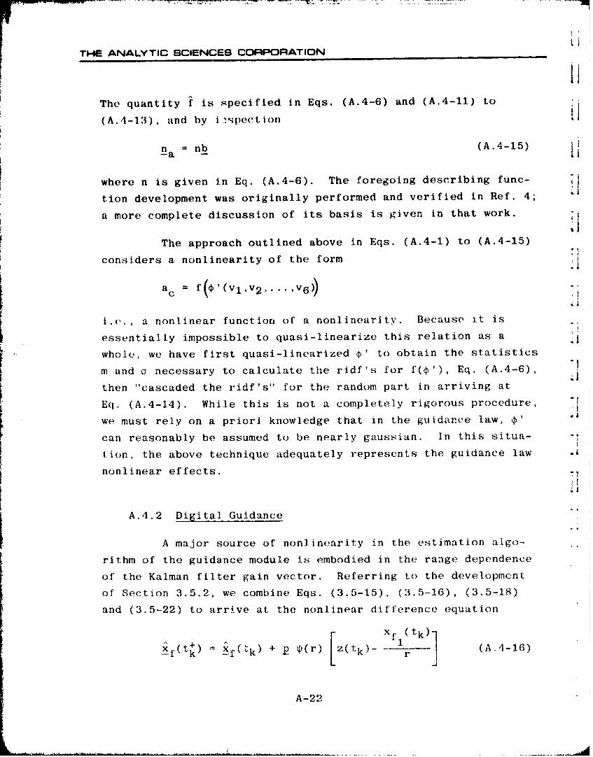
t i
THE ANALYTIC SCIENCES CORPORATION
i1ii
The quantity f is specified in Eqs. (A.4-6) and (A.4-11) to
(A.4-13), and by i .•lpection
n =nb (A.4-15)!!a
where n is given in Eq. (A.4-6). The foregoing describing func-
tion development was originally performed and verified in Ref. 4;
a more complete discussion of its basis is given in that work.
The approach outlined above in Eqs. (A.4-1) to (A.4-15)
considers a nonlinearity of the form '1
ac = f(V(VlV2...v6))
i.e., a nonlinear function of a nonlinearity. Because it is
essentially impossible to quasi-linearize this relation as a
whole, we have first quasi-linearized ý' to obtain the statistics -Im and a necessary to calculate the ridf's for f(f'), Eq. (A.4-6),
then "cascaded the ridf's" for the random part in arriving at
Eq. (A.4-14). While this is not a completely rigorous procedure,
we must rely on a priori knowledge that in the guidance law, ¢'
can reasonably be assumed to be nearly gaussian. In this situa-
tion, the above technique adequately represents the guidance law
nonlinear effects. -•
A.4.2 Digital. Guidance
A major source of nonlinearity in the estimation algo-
rithm of the guidance module is embodied in the range dependence
of the Kalman filter gain vector. Referring to the development
of Section 3.5.2, we combine Eqs. (3.5-15), (3.5-16), (3.5-18)
and (3.5-22) to arrive at the nonlinear difference equation
SXfl (tk)l
Xf(t+) 4(k) + p p(r) Z(tk)- (A.4-16)
A-22
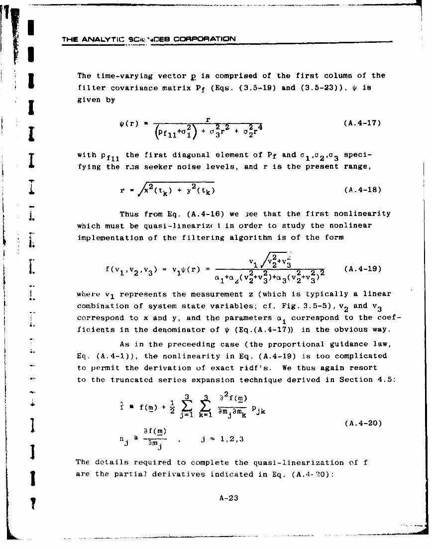
THE ANALYTIC ,CitdCES CORPORATION
The time-varying vector p is comprised of the first column of thefilter covariance matrix Pf (Eqs. (3.5-19) and (3.5-23)), q) is
given by
rp(r) 2 2 + 2r4 (A.4-17)
(Pfilu~ 3- 2T
with Pfll the first diagonal element of Pf and 01,G2,o3 speci-
fying the r..as seeker noise levels, and r is the present range,
N" r = 2tk) + 2tk) (A.4-18)
Thus from Eq. (A.4-16) we 3ee that the first nonlinearity
which must be quasi-lineariz( i in order to study the nonlinear
implementation of the filtering algorithm is of the form
v1 v+v 'f(vv = vq)(r) 2 2 2 2 2 2 (A.4-19)
1 +a 2( v 2 +v 3 )+ot 3 (v 2 +v 3 )
where v 1 represents the measurement z (which is typically a linear
combination of system state variables; cf. Fig. 3.5-5), v 2 and v3
correspond to x and y, and the parameters ai correspond to the coef-
ficients in the denominator of * (Eq.(A.4-17)) in the obvious way.
As in the preceeding case (the proportional guidance law,
Eq. (A.4-1)), the nonlinearity in Eq. (A.4-19) is too complicated
to permit the derivation of exact ridf's. We thus again resort
to the truncated series expansion technique derived in Section 4.5:
2f FA f(m)+k amam Pjk
~J=1ik-1 j k
af(m) (A.4-20)
n. =- i = 1,2,3mj
The details required to complete the quasi-linearization of f
j are the partial derivatives indicated in Eq. (A.4-20):
A-23
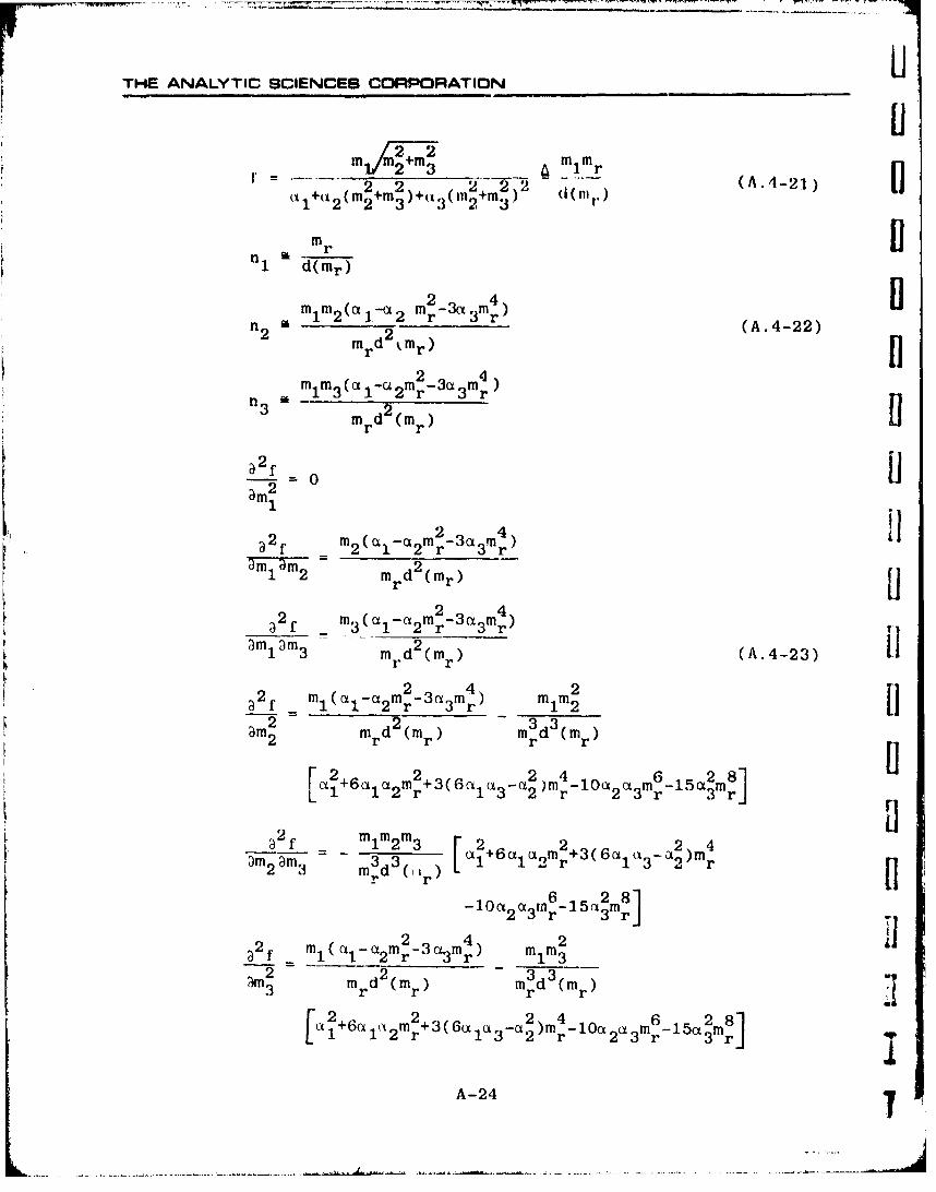
THE ANALYTIC SCIENCES CORPORATION
J-2- 2 mm
in 3 +mr mm+=2 2 2 3 . 2 2 (A.4-21)
~1+(12 m2 +m3 )+ 2 3 (+m2+m 3 ) d(ni+r)
m r r"1 d(mr)
m m2( .. t 2 m2 3t ~4
n 14 2 ('1.'2 mr =' in 4) (A.4-22)mrd 2 mr)
mnm 3 (11(ct,-.m 2- m3 r)
mrd (mr)
r_ r2-- = 0
2 2 3 m) 21
am m d 2 (ma II2 2 4 2
2f, mi (cxi-c 2 mr-3ca3 mr) mlm2
Ti'2md 2 (m
am2 mrd2 (mr) mrd3 (in) )
[cm+6cmlc 2 m2+ 3( 6c• 1 (•3 -c2 )m4r-1O2 m6-15ct2m8]
r r)H
2 f mm 2 m3 2 r 2 2 4
am2 -m re3 3 ( L' )Cl+6Ctl 2mr+ 3 ( 6 al•- )rH
11(m3 Ind 2'r -lctcmr 3(A.4-23)
-lo~am6-1532m8]
2_ 4 2
a 2 f IM m1(a 1-ct2 m r3a 3m)r 1 3
2 3•3am2 mrd2(mr) mrId (m)
cx 2 +6ot a m 2r+ 3 (6 6(X -a 3- 2 ) mr 4_1Oa I _ 5 2 m"
A-24 X2

THE ANALYTIC SC'ENCE8 CORPORATION
"j IThese relations complete the quasi-linearization of Eq. (A.4-19)
according to Eq. (A.4-20).
The second nonlinearity in Eq. (A.4-16) is of the form
1' • (r) v- f(v,v 2 ,v 3 )2 r Vl - 2 1 2 22 (A.4-24)1 la2( 2 3 3 2 -2
where v 1 now represents the first filter state, xfl. As above,
SmI m11 1(A.4-25)
a +a m2++a m4 d(mr)1 2 r 3 r r
1. _
1.1.. nI 1 d(mr)
2zlm2 (a a+2a m 2)
2" n2 " 1 2 2 r (A.4-26)J, d2 (mr)I
"2 2m2m3 (ct 2 -2ctm2 )
d 2(mr
"A 2
a f
"am12
.. • 2 f2m 2 (a 2+ 2 a 3m 2 )2m 2
am Ilam2 d 2(mr)
32m3(a2+2a m (A.4-27)
am-am3 d 2 (mr)
S2 f _ 2 ml(a 2 + 2 otm2 + 8m1 m2 r 2__ ,r [(a2_al )+3 ~m ra2+0Lmr)
am2d2 (m3 2 1a3 UIa3 r 2 -&3I
2 d(mr) d (M
A-25,On
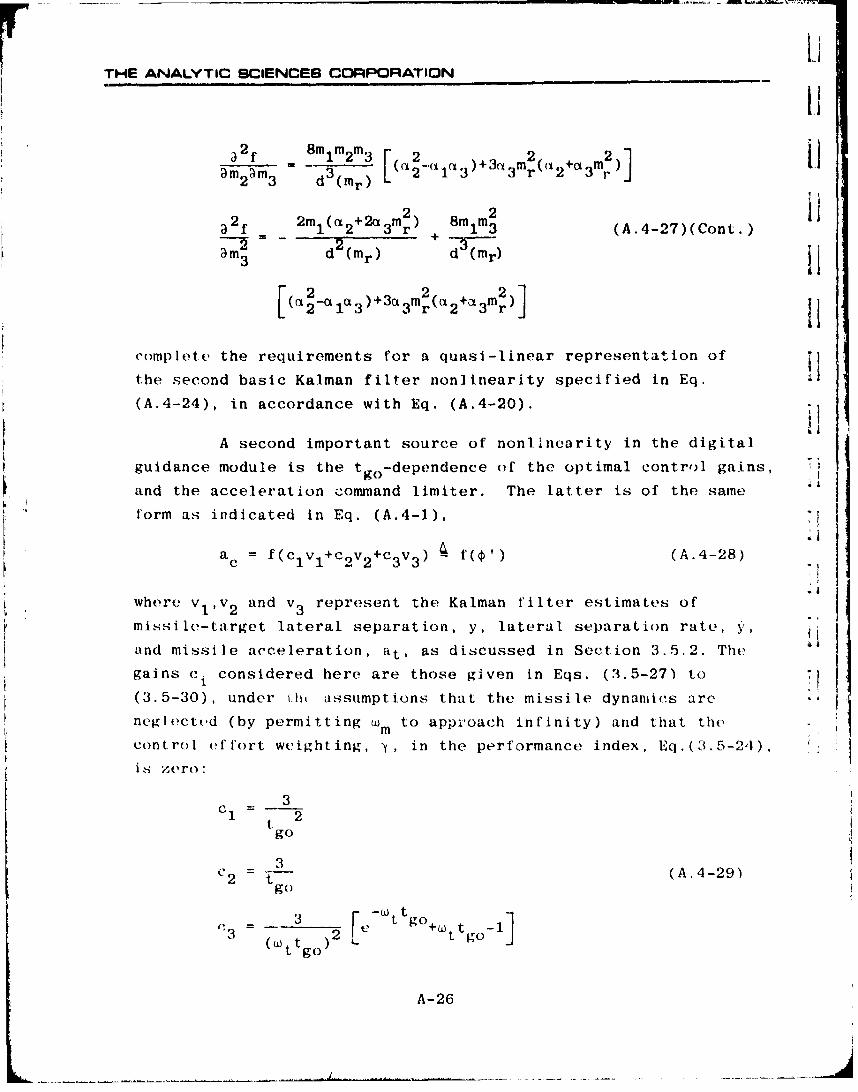
r LiTHE ANALYTIC SCIENCES CORPORATION ,Ii
a__2_f 8m 1 m2 m3 [ 2 2] 2am am = (a 2 -_.(% 1iQ 3 + +3a 3 mr (a• 2+0L 3 )am 2 m3 d 3 (mr)
222 2m 3 r 8M m2 +m(2+
2 a 3 mr 1m 3 (A.4-27)(Cont.)
2+am" d (mr) d (mr)
(a2_a a )+3a m 2r( 2a 32) I
[2( 13 m2r 2+0t 3mr
complete the requirements for a quasi-linear representation of pthe second basic Kalman filter nonlinearity specified in Eq.
(A.4-24), in accordance with Eq. (A.4-20).
A second important source of nonlinearity in the digital
guidance module is the t go-dependence of the optimal control gains,
and the acceleration command limiter. The latter is of the same
form as indicated in Eq. (A.4-1),
a= f(c 1 vI+Cav 2 +2c3 v 3 ) f() (A.4-28)
where v1 ,v 2 and v3 represent the Kalman filter estimates ofmissile-target lateral separation, y, lateral separation rate, V, -,
and missile acceleration, at, as discussed in Section 3.5.2. The ,
gains c. considered here are those given in Eqs. (3.5-27) to
(3.5-30), under th, assumptions that the missile dynamics are -,
neglocth'd (by permitting wm to approach infinity) and that the
control effort weighting, in the performance index, Eq.(3.5-24),
is zvro:
3el 1 2
tgo
3c 2 -t (A.4-29)go
Pa 3 3atg) e- g°+a t tgo- 1
A-26

THE ANALYTrIC SCIENCES CORPORATION
The gain 1 can reasonably be simplified by taking the, first 53 I-Wttgterms of the expansion of - ,ti.e.,
c a 3 1[ -2 ttgo + (Wt (A.4-30)
T
is a good approximation until the last fraction of a second of
an engagement and is more readily implemented in the guidance
module.
In order to estimate t, th- diigital system may hold
the range from the previous measurement, rk-l, and difference
it with the present value, as indicated in Eq. (3.5-32), viz.
so V 2+-V2 (A.4-31)
I. where v 6 represents the digital state holding rkl and v2+v26 - 4 5is the present rangc in cartesian coordinates in the state vec-
tor formulation.
Combining Eqs. (A.4-27) to (A.4-30) yields the completenonlinear representation of the acceleration command limiter
input:
3v1 [ /-2v+~ 2 3 2 [-~~
222( + 22!T('v 4 +v 5 v 2+v2v4s +
2_ 2 2+3 45 + T A 5
S~(A.4-32)
A-27
4 5
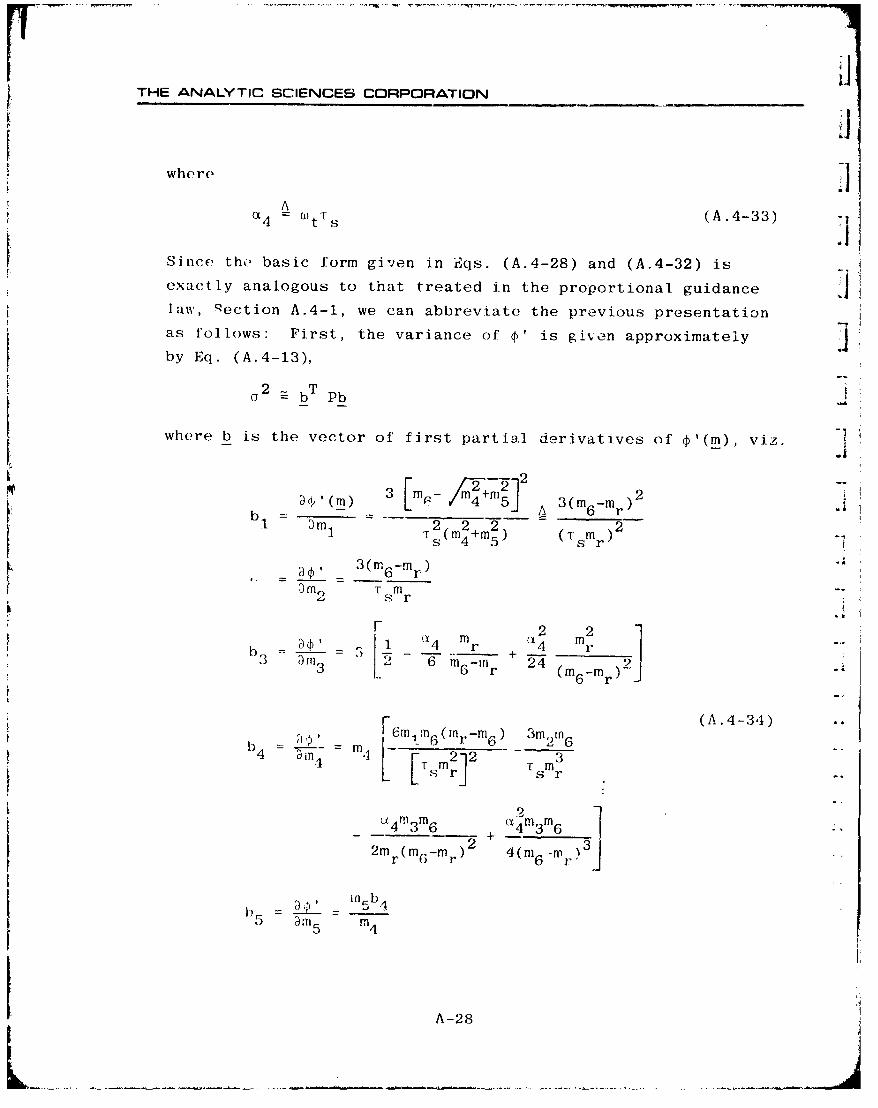
THE ANALYTIC SCIENCES CORPORATION
JIA
W4 t'rs (A. 4-33).-
Since the basic form given in Eqs. (A.4-28) and (A.4-32) isexactly analogous to that treated in the proportional guidance i
law, qection A.4-1, we can abbreviate the previous presentationas follows: First, the variance of ¢' is giveon approximately
by Eq. (A.4-13),
SbT Pb
where b is the vector of first partial derivatives of ý'(m), viz.
S/_-l_72-mm ni' m 3(m+nInJ2
,( 3 mA 3(m 6 -m)b I Din 2 2 2) 2
(m4 +m 5 ) (smr
3 (rn6rn)_ 6-r)3 rnT mn
s rhm2--
F 2 2b~ +23 - 3 6 m6-rn 24 (m 6 mr) 2j
3 6- r
rn 1 .fl 6 )3m ~(A.4-34)
b4 - bi1-m4 [cmrn6 26"
6min rn - 23mi
M 4 63r6 a 4 m3 m6 2.
2mr(m-m)2 4(m rn-m)3j
I5 Din5 m 4
A-28
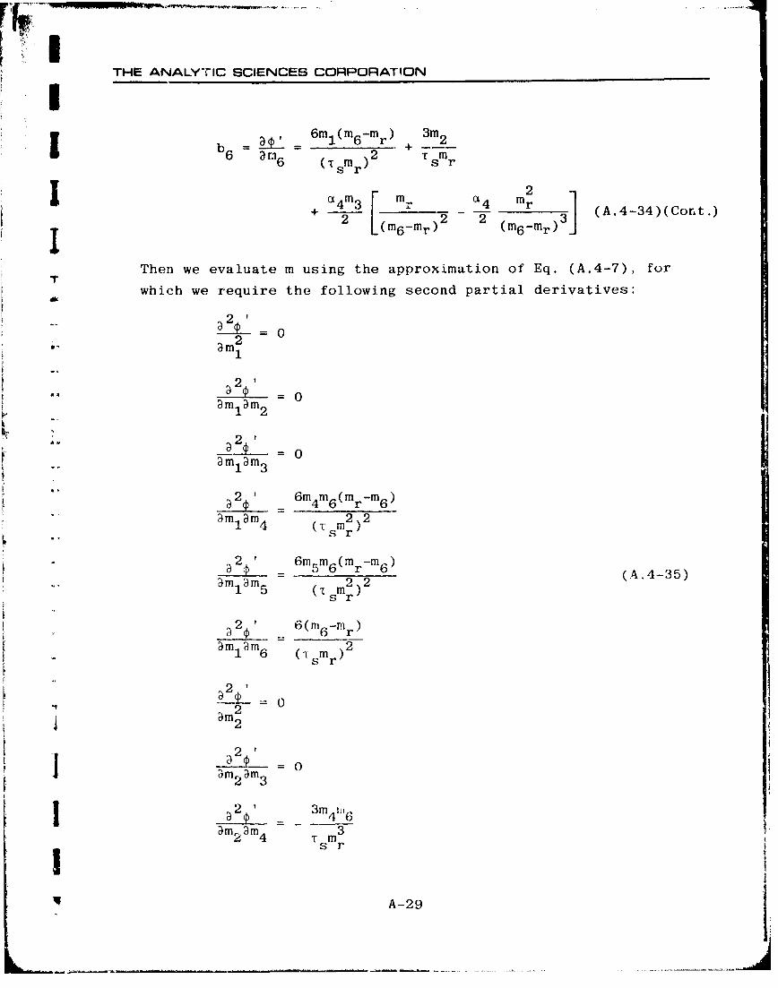
THE ANALYTIC SCIENCES CORPORATIONI6m (m -M 3m
b6 = 6 m(m 6 -mr) 2b6 an6 (Tsmr)2 Tsmr
2a m [ _ mr m
+ 4 3 2 r 3 (A.4-34)(Corxt.)
Then we evaluate m using the approximation of Eq. (A.4-7), forTwhich we require the following second partial derivatives:
2'
2'
3m1 ~m2
S2 '
a 2.. 3lm
2' 6m4 m6 (mr -m6 )"mm 4 ( rn2 ) 2
1~~ 4 s mr)
""2'2 - 6 m5 m6 (mr-mr6 ) (4.4-35). m am 2 2(.4-5
1 5 ( mr)
2' 6(m 6 -mr)16 (mr)
s r
2' _- 0o2
.22 0
am am2 3
_ 23 4116am2 am 4 m3
s r
A-29 I

THE ANALYTIC SCIENCES CORPORATION
S2' _ 3m m6i
m 5 56am Dn325 T M
2'a)m2 am6 sm mi"SS •
am 2m3
2 3 mm 6
1+ - m -m
am 3 am4 2mr(m 6 -m) 3 6]
2' cxm M, I 1
m 2r 6-m) 1+ mr-m
a23 €m 2(mmr) m-! r (A.4-3£)(Cont.,) Ai3m3Dm5 2m(m6mr)3 2
2Am 45 3 2 5
4m 2 m(4 m5 D i4n m 5,
2 m m5 [ -6m lm6 (f4m6 - 3m. ) 9m2m6 (X 4 m3 m6 i
am4 Din5 4 (T m3r 2 TM5 2(m6_mr 3-S star 6-
i 3mr-m 6 3_4 1m2 (m.. -.
r 2(m 6-mr) r)
2 ' [6m (m-2m6 ) 3m2 a4 M 3 (m 6 +mr)
I 3,D11 4 01116 4 (T in2 ) 2r in 2mn (m -m 3
2a 4 m23 (2m 6 +m)
4(m 6 -Mrn) 4
A-30
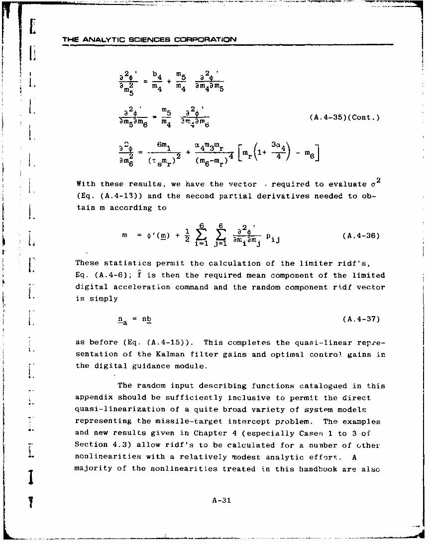
•.a~ -,•. .. • r.. ,-, -- .,r r ,-n --.w • •-,•• •• -- , • • ,,, •,•.... • "-•I.~w w. ~ ~r ~r- -- " -. , '.r'r 'W V' f r..v,• , -Cfl "". .. - r= rw hyr.. r " II P j U
THE ANALYTIC SCIENCES CORPORATION
Sa2 ' b4 m5 a2•b'124b + -5
a 2 m am amm5 4 4 4 5
a2.435m5 a21tn.am5 am 6 m4 34am (A.4-35)(Cont.)
1.0 6m 0 m m
m 2 2 T 2 4r 4 mr+ -m6
Sam sm (m 6 -mr)
F 2With these results, we have the vector required to evaluate a(Eq. (A.4-13)) and the second partial derivatives needed to ob-
tain m according to
6 6 2
m= = am(amJ Pj (A.4-36)
F oThese statistics permit the calculation of the limiter ridf's,
Eq. (A.4-6); f is then the required mean component of the limited
digital acceleration command and the random component ridf vector
is simply
n = nb (A.4-37)-a -
as before (Eq. (A.4-15)). This completes the quasi-linear repre-sentation of the Kalman filter gains and optimal control. gains in
the digital guidance module.
The random input describing functions catalogued in this
Sappendix should be sufficiently inclusive to permit the directquasi-linearization of a quite broad variety of system models
"representing the missile-target intercept problem. The examples
and new results given in Chapter 4 (especially Cases 1 to 3 of-, Section 4.3) allow ridf's to be calculated for a nunber of other
nonlinearities with a relatively modest analytic effort,. Amajority of the nonlinearities treated in this handbook are also
A-31

ITHE ANALYTIC SCIENCES CC.JPORATION
of common occurrence in other nonlinear system models, so it is
our hope that Chapter 4 and this appendix will facil-itate the
use of CADET in other applications as well. 3
T
A
-r
4
A-32 J

THE ANALYTIC SCIENCES CORPORATION
[, APPENDIX B
EXTENSIONS OF CADET
1]- B.1 INTRODUCTION
We have indicated that there are situations in which the
"j basic CADET methodology is inadequate. As discussed in Section
4.2, the most common difficulty that arises is that the random- component of a nonlinearity input, vi, has zero correlation with
the output, z = f(vi). For example,
are cases for which
EE vi] O
where vi is a gaussian random variable. In this event, the ran-
dom input describing functions (ridf's) for the random compo-
nent -- which by definition only capture the nonlinearity input-
* output relations for the correlated components of the output --
are identically zero. If this problem occurs in a primary trans-
mission path of the system model, a statistical analysis using
the basic CADET approach may be significantly in error.
A practical resolution of the difficulty described above
has been proposed in Ref. 20. It is based on the selective
SB-i
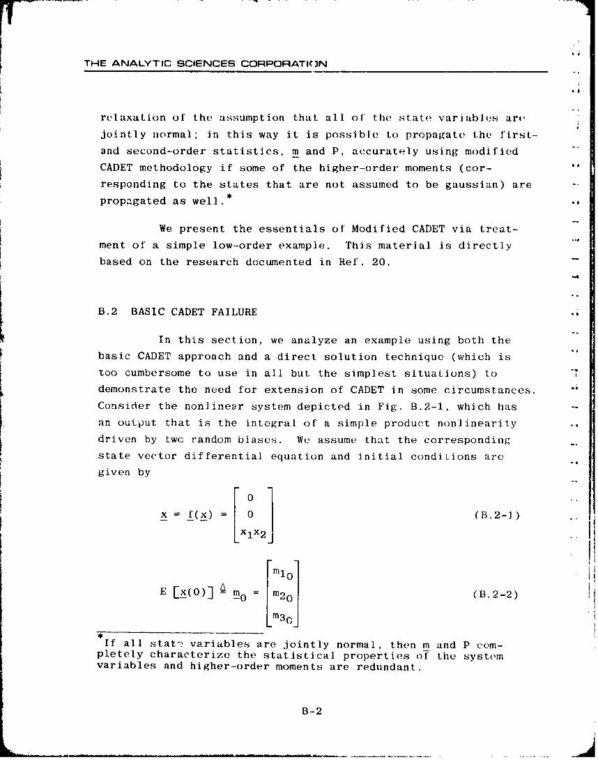
THE ANALYTIC SCIENCES CORIORATION
relaxation of the assumption that all of' the state variables are
jointly normal; in this way it is possible to propagate the first-
and second-order statistics, m and P, accurately using modified
CADET methodology if some of the higher-order moments (cor-
responding to the states that are not assumed to be gaussian) are
propagated as well.*
We present the essentials of' Modified CADET via treat-
ment of a simple low-order example. This material is directly
based on the research documented in Ref. 20.
B.2 BASIC CADET FAILURE
In this section, we analyze an example using both the
basic CADET approach and a direct solution technique (which is
too cumbersome to use in all but. the simplest situations) to
demonstrate the need for extension of CADET in some circumstances.
Consider the nonlinear system depicted in Fig. B.2-1, which has
an output that is the integral of a simple product nonlinearity
driven by twc random biases. We assume that the corresponding
state vector differential equation and initial condiLions are
given by
x = f(x) = (B.2-0)XlX2
[M10
E [x(O)J 0 = in2 0 (B.2-2)
Lm3
If all stat-, variables are jointly normal, then m and P com-pletely characterize the statistical properties of the systemvariables and higher-order moments are redundant.
B-2
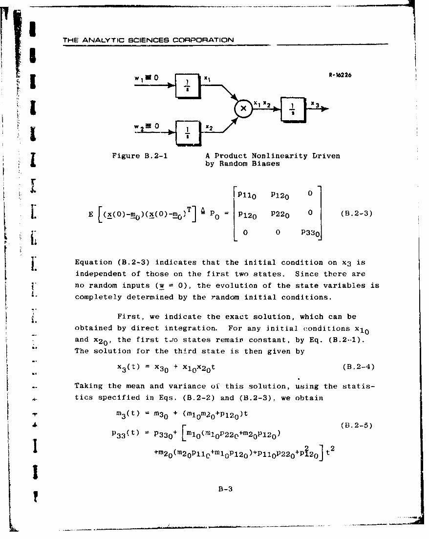
THE ANALYTIC SCIENCES CORPORATION
I Rt-16226
X KI• X2 l
Figure B.2-1 A Product Nonlinearity Drivenby Random Biases
.P10 P12 0 0
]L E [(•(0)-mO)(x(0)-)T] A P0 = [P120 P22 0 0 (B.2-3)
0 0 P330i
]I Equation (B.2-3) indicates that the initial condition on x3 isindependent of those on the first two states. Since thore are
no random inputs (w = 0), the evolution of the state variables is
"completely determined by the random initial conditions.
First, we indicate the exact solution, which can be
obtained by direct integration. For any initial. conditions Xlo
and x 2 0 , the first t.o states remain constant, by Eq. (B.2-.1).
The solution for the third state is then given by
- x3 (t) = x 3 0 + x 1 0 x 2 0 t (B.2-4)
I . Taking the mean and variance of this solution, using the statis-
•. tics specified in Eqs. (B.2-2) and (B.2-3), we obtain
m3 (t) = m3 0 + (rnl 0m2 0 +Pl 2 0 )t
P 3 3 (t) = P3 3 0 + [m1 0 (m1 0 P2 2 0 +m2 0 P1 2 0 )
+m2 0 (m2oPll+ml0 P1 2 0 )1Pll 0 P2 2 0 +Pi 2 0 ] t 2
B-3
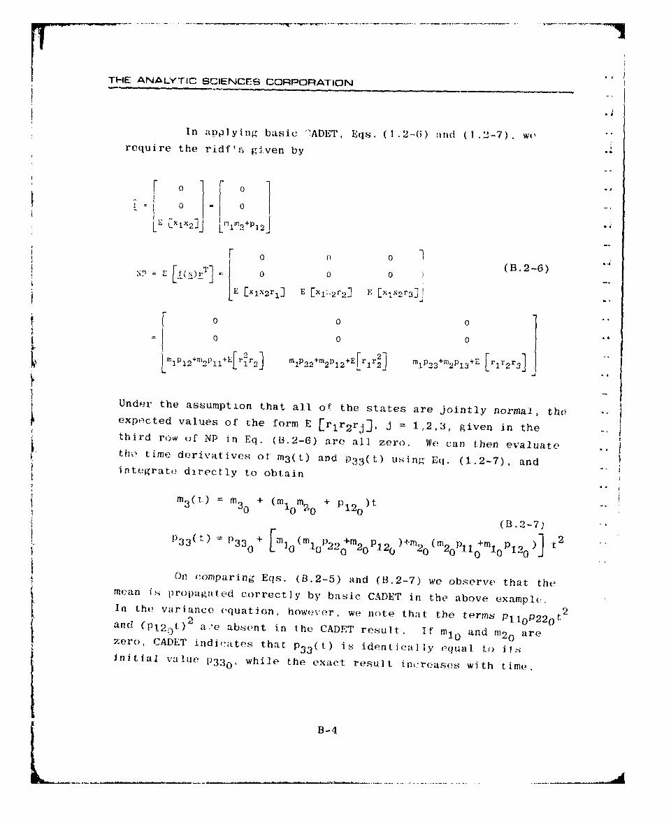
THE ANALYTIC SCIENCES CORPORATION
In applying basic "ADET, Eqs. (1.2-6) ;ind (1 .-- 7). w"require the ridf'l, given by
0 0
0
L' E L M..2 +p 1 2
N2- t~~r]0 0 (13.2-6)
LE Ex1 , 2 r1 J E [x 1 .-2 r 2 ] E [x',x2r 3 ]J -
0 0 01S0 0 0
rnlP12" 112 1+ 1 -'Jr2 ] m 1P 22 +m2 P 1 2+E[rlr] m P1 2 3 1 2P 1 3+E [rir 2 r 3 ]
Under the assumption that all of the states are jointly normal, the.,exp,'cted values of the form E [rlr 2 rj], j 1,2,3, given in the
third row of NP in Eq. (8.2-6) are all zero. We can then evaluatethe time derivatives of m3 (t) and P 3 3 (t) using Eq. (1.2-7), andintegrate directly to obtain
m3 (t) = m3 + (m1 m2 +m0 (o20 P10
(B.2-7)
P 3 3 (t) P330 + [t 1 0(m21 201 m2 0P01 )+P20 (mi2 0PI1 +m1 oP 1 2 )] t 20
On 1-omparing Eqs. (8.2-5) and (B.2-7) we observe that themean i:i propagated correctly by basic CADET in the above example.
In the variance equation, however, we note that the terms p4ioP220t2
and (Plot)2 a.'e absent in the CADET result. If mlo0 and 11120 arezero, CADET indictates that P 3 3 (t) is identically equal to ilsinitial value P33 0 , while the exact result increases with time,
B-4

THE ANALYTIC SCIENCES CORPORATION
P33(tIMi =0 2 + P + P 2 2
I In the general case (nonzero means and correlated states driving
the product nonlinearity), then, CADET will do relatively well
L in estimating the variance of x 3 if
2 2 22m 1 0m2 0P 1 2 0 + m2 0Pl0 + M 1 0P 2 2 0 > P1 1 0P2 2 0 + p12 '(B.2-9)
This is a quite restrictive condition.
"As demonstrated in Section 1.2, CADET will propagate the
mean and covariance of the nonlinear system exactly if the ex-
pected values appearing in Eq. (B.2-6) are correctly evaluated.
Basic CADET does not evaluate these expectations appropriately
for the product nonlinearity just considered, because the proba-
bility density function of the product of two gaussian random
variables is clearly nongaussian. Thus x 3 cannot be assumed to
be jointly normal with x and x 2 without causing CADET accuracy
deterioration, except in cases that satisfy Eq. (B.2-9). An
approach for modifying CADET, which tends to eliminate this source
of error, is introduced and explained in the next section.
-i .B.3 TWO GENERALIZATIONS OF CADET
B.3.1 Exact Solutions via Higher Moment Propagation
Having motivated the need for generalizing basic CADET
by demonstrating its breakdown for a system having a product non-
lincarity, a technique for extending CADET is introduced using the
J sane example. Consider the problem originally posed in Section
B.2 -- the nonlinear system of Fig. B.2-1 driven by two random
.VS--
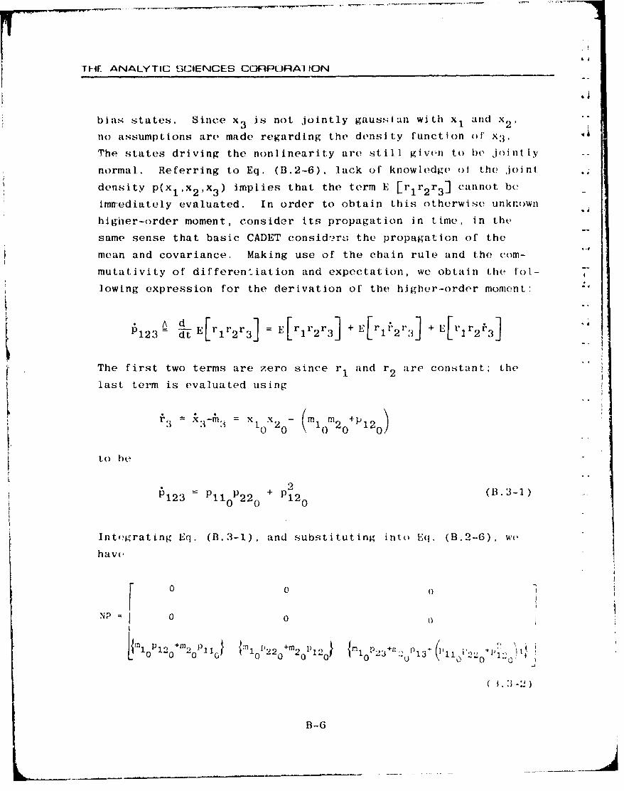
THF ANALYTIC SCIENCES CORPPLJRAI ION
bias states. Since x is not jointly gausslan with x and x2 ,
no assumptions are made regarding the density function o(f x 3 .
The states driving the nonlinearit~y are still given to be joint IN
normal. Referring to Eq. (B.2-6), lack of knowledge of the joint.
density p(xl,x 2 ,x 3 ) implies that the term E [r r 2 r 3 ] cannot be
immediately evaluated. In order to obtain this otherwise unknown
higher-order moment, consider its propagation in time, in the
same sense that basic CADET consid-ers, the propagation of the
mean and covariance. Making use of the chain rule and the com-
mutativity of differentiation and expectation, we obtain the tol-
lowing expression for the derivation of the higher-order moment:
12^~E~~~~ dtd r"lE~~~ 1 +E rriK1A123 = = 2 + 3rJ + L[ J
The first two terms are zero since r 1 and r2 are constant; the
last term is evaluated using
x1 -m m x + )3,, 1 03•: 2 X~ 0 - (mlom2 0+12 0)
t o 1)e * 2
123 = l po 2 2 0 + p 1 2 (13.3-1)0 0 0
Integrating Eq. (B.3-1), and substituting into Eq. (B.2-6), wehave
F 0 0 0
\P"0"0 0 o
B-6
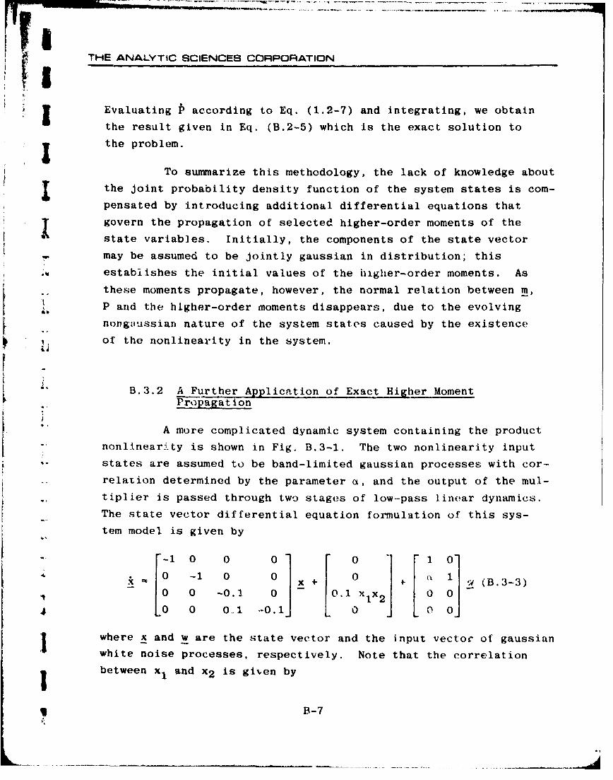
THE ANALYTIC SCIENCES CORPORATION
i iIf Evaluating P according to Eq. (1.2-7) and integrating, we obtain
the result given in Eq. (B.2-5) which is the exact solution to
the problem.
To summarize this methodology, the lack of knowledge about
the joint probability density function of the system states is com-pensated by introducing additional differential equations that
T govern the propagation of selected higher-order moments of thestate variables. Initially, the components of the state vectormay be assumed to be jointly gaussian in distribution; this
establishes the initial values of the higher-order moments. As
these moments propagate, however, the normal relation between m,
P and the higher-order moments disappears, due to the evolvingnongaussian nature of the system states caused by the existence
of the nonlinearity in the system.
B.3.2 A Further Application of Exact Higher MomentPropagation
"A more complicated dynamic system containing the product"nonlinearity is shown in Fig. B.3-1. The two nonlinearity inputstates are assumed to be band-limited gaussian processes with cor-relation determined by the parameter a, and the output of the mul-
tiplier is passed through two stages of low-pass linear dynamics.The state vector differential equation formulation of this sys-
tem model is given by1 [ 0 0 01 0 1 0[ i- =0 -1 0 0 [ + (0 1 (B.3-3)
0 0 -0.1 0 0.1oXl1x 2 00[o 0 00.1 -0.1 L 0 J L 0 ]
where x and w are the state vector and the input vector of gaussianwhite noise processes, respectively. Note that the correlation
between x 1 and x 2 is given by
B-7

THE ANALYTIC SCIENCES CORPORATION
. i
Figure B.3-1 Dynamic Sys t.in Wit h i Product-o t-Stai•(, Nonl inearity
2 ~t
12 = (0 (B. 3-4b)
so the degree of' correlation is directly proportional to 'FilTe,
state variable initial conditions were chosen to be zvtro; theF.n
given the constanr nt in means, byi and spynctral dnAities, (oi
(refer to Eq. (1.1-2)), the. statistics of the sdtatles drivind the
multiplier c0an be directly oibtained to be
- 2t
-t-
In2 )2 + ab 1)(1 e- t
P 22 = ((12 + .*qj)(1 -e "')!
The• stattistical analys•is of' the, y• (, ,lopictodl ii) Fij!.
B.3-1 waý, varried out in Ref. 20 by applying ha.si( CADET, oxa,-L
high er m o)m ent p r'opagrat i(n (h erea ft e-r design at e•d Ml l') . and th e,
m()nt e, car l o m e'thod (200 tr ia ls ). in th e, va~ w.-(' p rose; nt o~d |l ,r o,,
B-8
THE ANALYTIC SCIENCES CORPORATION
!a is taken to be 0.1, and the input white noise processes were
chosen ir have means and spectral densities given by bi = 0.01,
qi = 1.0 respectively. Consequently, from Eq. (B.3-5) we observe
that the means are much less than the rms values, so, as indicated
in Eq. (B.2-9), it would be anticipated that CADET would be quite
inaccurate in this circumstance. The results are portrayed in
Fig. B.3-2; since the driving states, xI and x 2 , are jointly
gaussian, we confine our attention to the evolution of a3 and 04
with time. Observe that the HMP result is exact, as verified by
the monte carlo dala, while the basic CADET analysis is completely
inadequate in its projection of o3 and i4 versus time.
For the above example the HMP analysis only entailed the
propagation of two higher-order moments, E [r 1 r 2 r 3 ] and E Er 1 r 2 r 4 ].
, i'he computer time expenditure was thus nearly identical with that
"of basic CADET; the monte carlo analysis required 26 times the
CADET computational expense.
A question of some importance regarding the general prac-
ticality of HMP concerns the impact of increasing the complexity
of the system before and after the nonlinearity. As demonstrated
in Ref. 20, simply introducing coupling between states 1 and 2,
e.g. replacing the first two state variable differential equations
in 2q. (B.3-3) with
"A I alx 1 + a 1 2 x2 4 WI
"k2 a 2 2 x2 + W2
ircreases the number of higher order moments that muLst be propa-
gated from 2 to 4. A similar increase in computatic.nal complexity
occurs when the system is made more complicated foilowing the non-
linearity. Thus the analysis of high-order closed-loop systems
via HMP may be impractical.
IB-9

THE ANALYTIC SCIENCES CORPORATIOPi
0.12 It.1 , 300
x0.08 MONTE CARLO, 200 TRIALS
L-0
> 0.n4 '0f4EXACT HIGHER
SMOMENT PROPAGATIONBASIC CADET
00 10 20 30 40
TIME, t (sec)
(a) The rms Value of x3
0.12
EXACT HIGHERMOMENT PROPAGATION
"• 0.08
0w
S0.04 O, 200 TRIALS
00 10 20 30 40
TIME, t (sec)
(b) The rms Value of x4
Figure B.3-2 Simulation Results for a System Containinga Product-of-States Nonlinearity
B-10
THE ANALYTIC SCIENCE8 CORPORATION
J B.3.3 Modified CADET
The Modified CADET methodology suggested in Ref. 20
serves the purpose of providing a significant increase in the
accuracy of CADET without the great increase in computational
* burden that may be necessitated in using HMP to treat high-order
systems, especially those in a closed-loop configuration where
I all or nearly all of the system state variables may be nongaussian.
The application of Modified CADET to the simple system
treated in the preceding section (Fig. b.3-1), containing a pro-
duct nonlinearity followed by two stages of linear dynamics, is
summarized by the following basic steps:
- Relax the gaussian assumption only on that& •; component of the state vector "nearest" the
output of the nonlinearity (i.e., x3 in
Fig. B.3-1); retain the assumption of jointnormality on all other states.
•Develop expressions for the derivatives ofall resulting unknown higher-order moments
ýJ appearing in the evaluation of the expectedvalues in f and NP, Eq. (1.2-6) (as inEq. (B.2-6)).
a Integrate these derivatives along with thederivatives of the system mean and covari-ance from assumed initial values.
The rationale behind this selective assumption of joint normality
is states more than a few integrations from the
nonlinearity (e.g., x4 in Fig. B.3-1) can be assumed to be jointly
normal with respect to other gaussian states (e.g., x 1 and x 2 in
the same figure), for reasons discussed in Section 1.2.
To demonstrate the usefulness of Modified CADET, we treat
the same example as above (Figs. B.3-1 and B.3-2) under the assump-
tion that x 4 is gaussian. Then E [r 1 r 2 r 4 ] is identically zero, and
only one higher-order moment is propagated. The corresponding time
IS~B-li

THE ANALVTIC SCIENCES CORPORATICN
history of 04 is compared with the HMP result in Fig. B.3-3;
clearly it provides a close approximation to the exact solution.
It-| (,i'99
0.10
EXACT HIGHER
MOMEN7 PROPAGATION0.08 (Figure B.3-2)
X 0.06U.0
UiMOIFIED CADET
> 0.04
0.02
10 20 0 40
TIME, t (sec)
Figure B.3-3 Modified CADET Solution For theSystem Shown in Fig. B.3-1 WithOnly One State Assumed Nongaussian
Modified CADET represents a methodology which potentially
broadens the usefulness of the CADET concept, permitting Its
applicability to a wider class of nonlinear systems. For the low-order examples presented in this appendix, Modilied CADET has
clear-cut advantages, and we anticipate that it will be a useful
method for improving the accuracy of statistical analyses for more
complex systems.
B-12
THE ANALYTIC SCIENCES CORPORATION
- APPENDIX C
THE MONTE CARLO METHOD: APPLICATION AND RELIABILITY
-i:[ C.I DESCRIPTION OF TIE TECHNIQUE
SI"The monte carlo method provides an approach for the
statistical analysis of the performance of a nonlinear system
with random inputs, based on direct simulation. t entails de-
termining the system response to a finite number of "typical"
initial conditions and noise input functions which are gener-
L4 ated according to their specified statistics. Thus, the infor-
mation required for monte carlo analysis includes the system
* model, initial condition statistics, and random input statistics.
The system model can be given in the form of a state
"vector differential equation,
I. = f( t)1)
where x is the vector of system states, • is a vector of random
inputs, and f(x,y,t) represents the nonlinear time-varying dy-
namic relationships in the system. We assume at the outset that
the elements of y are correlated random processes with deter-
ministic components that may be nonzero; in this case, a system
model of the form
-. = �f(x,t) + G(t) w(t) (C.1-2)
where w is the sum of a vector of white noise processes and a
j deterministic vector can generally be obtained that is equiva-
lent to Eq. (C.1-i), as discussed in Section 1.2. Henceforth,
I ...
~~~~ .... *.- ] - - - -
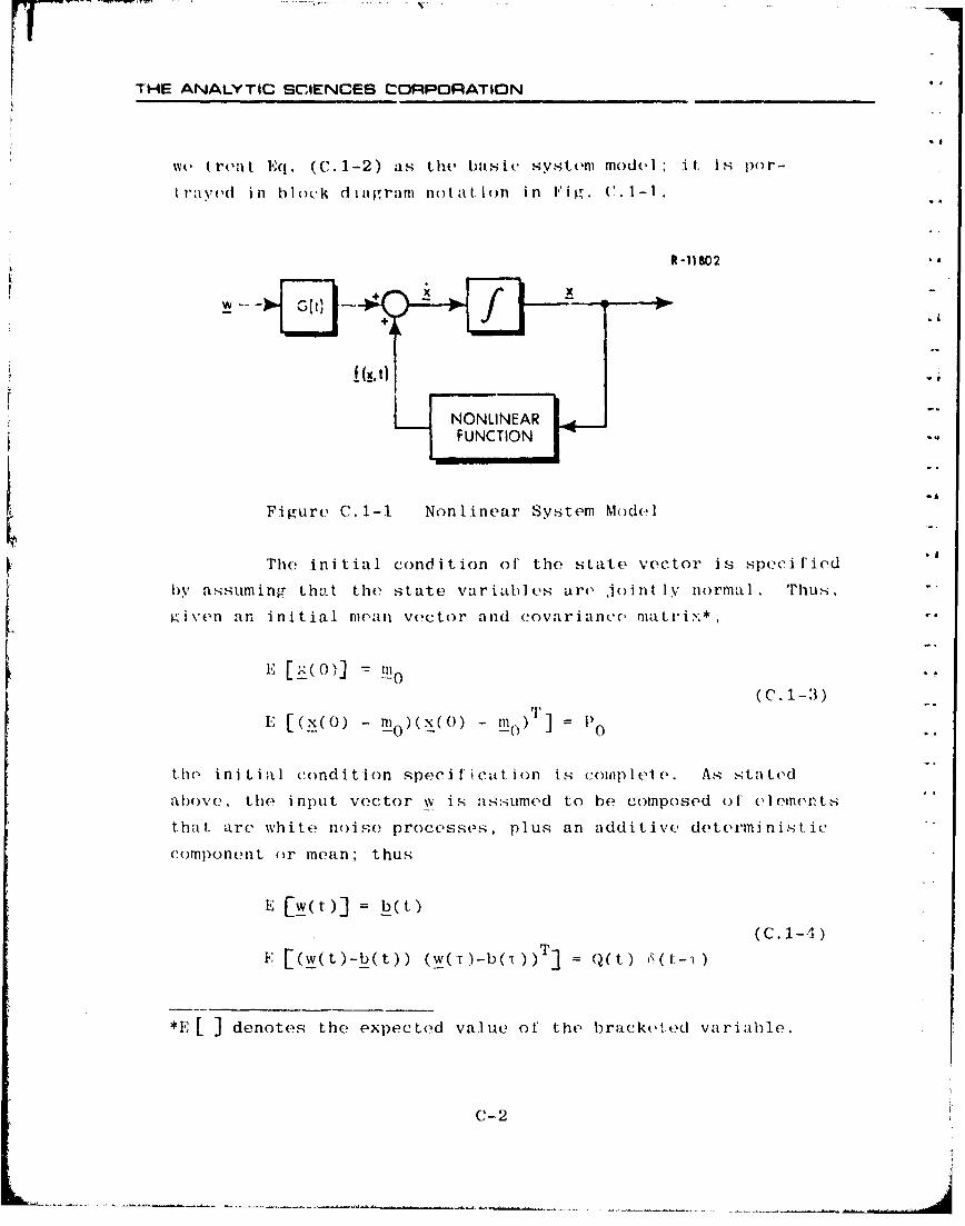
THE ANALYTIC SCIENCES CORPORATION
we treat E 1. (C.1-2) as the basic system model; it. is por-
traved in blo)ck diagram no )at.ion in F'ig. ( .-1
R-11802 .4
+ +
++1!(.~t). .
NONLINEAR
FUNCTION].
Figure C.1-i Nonlinear System Model
The initial condition of the state vector is specified
by assuming that the state variables are ,joint lv normal. Thus,
gi\'en an initial mean vector and (1covarianco matrix*,
E [x(O)] (C. 1-3)
E' : [(x (O ) - 10 )(x ( 0) - 11)1 ] = P0
tho initial condition specificat iion is complete. As stated
above , the input vector w is assumed to be composed of eleme, ts
that are white noise processes, plus an additive deterministi . "c
component or mean; thus
E [w(t)] = b(t) (C.1-4)S1; E (w( t)-b(t)) (w(T)-b(i)) T] Q(t) 6 ( 1 t"- )T
*E [ ] denotes the expected value of the bracketed variable.
C-2

S! I ~ THE, ANALYTIC ,SCIENCES COR:PORATION,
where Q(t) is the input spectral density matrix and the impulse
function 6(t-T) indicates that the input vector random components
have zero autocorrelation for t ý T; i.e., the quantity u(t) -
w(t)-b(t) is "white noise", as stated.
Given the above information, monte carlo analysis re-
quires a large number, say q, of representative simulations of
jthe system response, viz., the q-fold repetition of the following
procedure: First, an initial condition vector is chosen according
to the statistics indicated above; i.e., a random number genera-tor calculates the elements of a random vector x(O) based on Eq.
(C.1-3). Then a random initial input vector, w(O), is generated,
lb using the statistics given in Eq. (C.1-4)*. These vectors pro-
d vide the data for evaluation of i(O) in Eq.(C.1-2) which in turn
is used to propagate the solution from t-0 to t-h according to
any standard technique for the digital integration of a state
vector differential equation. Then, given x(h), simulation con-
tinues by the generation of a new value of the input noise vectorW(h), evaluation of k(h), numerical integration to obtain x(2h)
and so on, to the specified terminal time tf.
*We simulate white noise with spectral density matrix Q(t) by"using a random number generator to obtain an independent sequenceof random vectors u(kh), k-O,1,2,... satisfying
I.E[u(kh)] - 0
r~l 1E[R(kh)uT(kh)•J E Q(kh)
. Then we define u(t) by
A u(t) - u(kh), kh < t < (k+l)h
i where h is a small time increment. For h small (1/h much largerthan the bandwidth of the system in question), u(t) is an accu-rate approximation to a white noise process.
C-3

THE ANALYTIC SCIENCES CORPORATICN
PerfIorming (I imhependelnt simulationfs yields an ensemble
of state trajectories, each denoted x U) (t':xki)(O), wM i'(t)) to
stress the dc,)(ndence ol' the trajectory on the random initial
condition and noise Jnpa t sample function:
x(1 (t; x (1)( ), w(1) t)
x(2 (t; x (2)( ), w M()t) ; O<t--t (C.1-5)
x((])(t; x(0(), w(q)(t))
Each satisfies the state vector differential equation (Eq.
(C.1-2)) to within the accuracy of' the numerical integration
method used, and the ensembles of initial conditions, x (0),
anrd random inputs, w(i)(t), obey the statistical conditions
given in Eqs. (C.1-3) and (C.1-4), subject to the limitations
of' the random number generator employed. The mean m(t) and
covariance P(t) of the state vector are estimated by averaging
over the ensemble of trajectoris using the relations
A} 1 (i) ]
1=1si j' I(C,.1-6)
P(t) (x i) ( ) t)-n(t
whore r((t) and P(t,) denote the estimate(d vnilue,. 'Tao, essence
of the monto carl,) technique is illustrated in Fig. C.1-2.
In estimating P, we obsorve that it is necssary to divide by
((1-1), since the sample variance,q
is biased (Ref'. 8), i.e.,
E [11)] = -q q
C-.

THE ANALYTIC SCIENCES CORPORATION
~ SWI1~ TRMAL -19Ne. II
3 si shi 1 II I
0 U
i iTRIAL
STATISTICS 4NMATIM I )
IUITSI III INITMi.. PO10 IANDOM IC.,gCONDITION CIC Lh51S3 sPTstics
I7 -rý MNIC%
Figure C.1-2 Schematic Characterization of theMonte Carlo Technique
C.2 ASSESSMENT OF P'ICURACY -- CONFIDENCL INTERVALS
In order to assess the accuracy of the approximate sta-tistics given in Eq. (C.1-6), it is necessary to consider the
statistical properties of the estimates m(t) and P(t). To sim-
plify the notation, consider a scalar random variable y (e.g.,
the value of some system state variable at some time of interest),
and let m and p represent the true values of the mean and vari-
ance of y,
m - E [y]
"E yi)(C.2-1)-. p E p[y -m)•23
By performing one set of q monte carlo trials, we obtain a single
estimate of m and p, which we denote m and p. These estimates
are also randomr variables; that is, if another set of q monte
C! C- 5

THE ANALYTIC SCIENCES CORPORATION
carlo trials were performed independently of the first set., but
with the same statistics foIr the initial conditions and noise!
inputs, then a different ensemble of simulations results, and
different estimates for the mean and variance would bc obtained.
If q is sufficiently large, then we can invoke the central limit
theorem to Justify the assumption that the random variables m
and p are gaussian*, a..d thus that their distributions are
asymptotically specifi(ed by the following statisties for large
q (Ref. 21):
E[iii a rE~p] - p ..
(C.2-2)0 E[(_ii-m) 2 ] £mq ,
2 E[(p - p) 2 ] 11 4 pp qC
where p4 is the fourth central moment,
W4 a E [(y - M) 4 ] (C.2-3)
For many common probability density functions (pdf's), a con-st nt I o-xjst:x •,,h lh,
2
114 = ýP (C.2-4)
Table C.2-1 gives a summary of values of X, known :.s the kily'to-sis or excess of the. d.nfsi ty, I,,r ¾,,,l(' (O,,jf,,,t j Ir . Hi I ',
For q<20, it is necessary to assume that p has the chi squaredistribution if y is a gaussian variable (Ref. 22); if y issignificantly fnongaussian, the validity of the gaussian as-sumptJon for In and • may require considerably more than t wentytrials.
C-6

;r'THE ANALYTIC SCIENCES Co•PORArION
TABLE C.2-1
SOME COMMON PROBABILITY DENSITY FUNCTIONSSan,14179gl
DESIGNATION FUNCTIONAL GRAPHICALREPRESENWATON RWSENTATIONI
EXPONENTIAL .w) 6
-co << ( CO
•' ~~-OD < K< * COi • :-
TRIANGULAR 760 W1- 2.#n - /6,: x: f
01)
UNIFORM /iia, -,i - /3a m */3I
BIPOLAR 1/2 1.0j (€ ,ret). (-,n...) .-j
OFormula~ed to hove mean m oad stondord dovioaion a
of this type, we can express both of the standard deviations of
4. the estimated statistics given in Eq. (C.2-2) in terms of the
true variance, p, to obtain
(C.2-5)
The above discussion of the s•atistics of the gaussianrandom variable p provides the basis fcr determining a range in
the vicinity of P such that the true value of p is guaranteed to
7 C-7
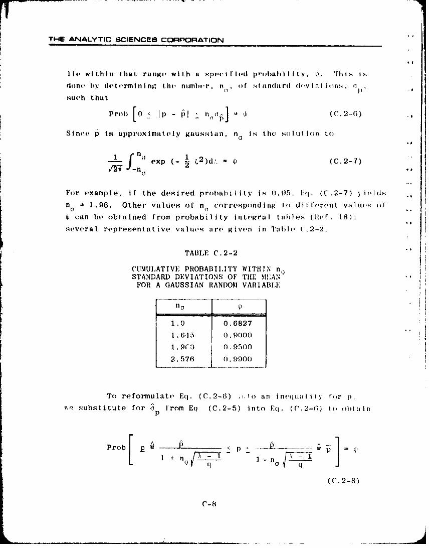
THE ANALYTIC SCIENCES CORPORATION
lit, within that rang, with it speci ied probability. q,. This is.
dom, hy de|termining the numlber, n , of' si an(Iar(I (flfviaft i•qs•, t(1 I) '-
such that
Prot) [0< l-f:l, no(C-2-6)
Sinnev p is approximately gaussiann, n Is the sol ut. iOIn to
n xp . 2 )d:. , (C.2-7) '
For example, if" the desired prohah i I ity is 0.95, Eq. (C.2-7) e (is
n 1,96. Other values of n corresponding to ditrorrent values o)I
4 can be obtained from probability integral tableNs (Ihf. 18);
several representative valuos are given in Table (,.2-2.
TABLE C.2-2
CUMULATIVE PROBABILITY WITHIN nSTANDARD DEVIATIONS OF THlE .MEAN
FOR A GAUSSIAN RANDOM VARI1ABILE
n o 4)
1.0 0.6827
1 . 6,5 0. 9000
1.9co 0, 9500
2.576 0.9900
To reformulate Eq. (C.2-6) iito an inequalit f()r p,%%, substitute for 3 from Eq (C,2-5) into Eq. (C.2-6) toh otain
p
Prob4 - p X n
(('.2-8)
('-8

ITHE ANALYTIC SCIENCES CODPORATION
!that is, the true value of p lies between the values p and p indi-
3cted in Eq. (C.2-8) with probability ý. Alternatively, in terms
of the estimated rms value of the variable. 3, we have the com-
I parable result
1*
"where o and • are given by
S..c
(C.?-9)
' -no q
The quantities a_ and • are referred to as lower and upper confi-
dcncc limits; the value of ý,• expressed as a percent is the degree
of confidence. Equation (C.2-9) demonstrates that the stand'rd
"deviation confidence limits can be obtained from u simply by using
"the multipliers p and P. The latter are fun-tiua' i only of the
kurtosis, X, the number of monte carlo trials, q, and the ntmber
A of standard deviations, n., required to achieve the desired de-
* gree of confidence.
The problem of miaking a reasonable choice ol A, which dE-
Spends upon the statistics of the random variable y, must be faced
before the confidence limit multipliers can be calculated. One
IJ option is to determine an approximate value of A by estimating
the fourth central moment using the q sample values of the vari-
able y, and calculating
S,4/ C-
S~C-9

S.... - .. • - -'-r*' . . ~ ....- : : • :,. = l.f W',.r jflo'' :r ,-•'--r -. - • .• •,: • . ... . W• • - ,
THE ANALYTIC SCIENCES CORPORATION
The value of X need not be kniown exactly, since the confidence limits(! and 0 are not extremely sensitive to errors in this parameter. Un- ifortunately, as we note in a subsequent example, a meaningful esti-
mate of A can often require several hundred trials. In the absence of •
reliable information about the higher central moments, it is fre-
quently assumed that y is gaussian; i.e., that X = 3. However, if H-there is any reason to believe that the pdf for y has abnormally
heavily weighted tails -- as in the case of the exponential dis-
tribution in Table C.2-1, for example -- then a larger value of X
may be required in order to arrive at a realistic assessment of
the accuracy of an estimated rms value obtained via the monte
carlo technique.
Values of p and p for X= 3 are indicated as functions of
the number of monte carlo trials in Fig C.2-1, for two typical
values of confidence. As an example of the significance of the
confidence interval, if we desire to have 99% certainty that a is
within 10% of the estimated value, 0; i.e.,
Prob [0.90a< a < 1.1 5] 0.99 (C.2-10)
then Fig. C.2-1 demonstrates that it is necessary to perform 440
trials; 256 trials suffice for 95% confidence.*
Figure C.2-2 shows the deterioration that occurs in the
accuracy of the monte carlo estimated standard deviation, for a
given level of confidence, if the kurtosis of the random variable
is greater than 3 due to y being nongaussian. We discuss an in-
stance where A 15 in Section C.3; in this case, even for 256
trials, the upper 95% confidence limit is 36% greater than the
estimated value of a.
Note that the bounds, p and p-• are not symmetric with respect toone; thus the point at which p crosses 1.1 determines the value ofq for which Eq. (C.2-10) is satisfied.
-- 10

;: ITHE ANALY'rIC SCIENCES CORPORATION
2.0 -_____
3Le
Uu
z
z Vowr Wmit.8 99% Confidenc.
Z 99%. Confidence
0
q 440
i< 1.0
for Lo-er Lima' r,95.'/Co.ndence
.I 99% Confidence
L100 300 500NUMBER OF MONWE CARLO TRIALS, c;
Figure C.2-1 Typical Confidence Interval Multipliersfor the Estimated Standard Deviation of"a Gaussian Random Variable (0 = 3)
The confidence interval calculation for the estimated
maan is quite direct, since Cf (Eq. (C.2-5)) is not a function ofm
the mean. The same value of n is obtained for the desired de-
gree of confidence (e.g., from Eq. (C.2-7), na = 1.96 for ý =
0.95 corresponding to 95% confidence), and the value* of p given
in Eq. (C.2-8) is used in deriving the result that for m and
m given by
3 While Crjj is given by /p/q in Eq. (C.2-5), the true value of p
is unknown. Thus a conservative (large) value of oam is ob-tained by using 1.
C-l1
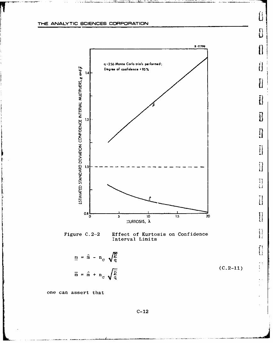
THE ANALYTIC SCIENCES CORPORATION
q ;256 Monte Carlo trio!t performied
14 ii
Degree of confidence s95%S1.4-
-J [3p
L 1.2zLU
o0
z0
0510 15 0I
:(URTOSIS, ,X
Figure 0.2-2 Effect of Kurtosis on Confidence i
Interval Limits
Ui,C 1.0
0.8i
(C.2-11) C si
m = m + n
one can assert that
C-12
. i

THE ANALYTIC SCIENCES CORPORATION
Prob [m < m < ] (C 2-12)
Here, we see that m and m cannot be readily expressed in termsA-
of a multiple of m.
The confidence limit concept developed above provides astatistical measure of the accuracy of the estimated mean and
standard deviation of a random variable obtained by using the
monte carlo method. It is only possible to assess the accuracy
of such estimates in a probabilistic sense; e.g., for 256 trials,
we can assert, for example, that an estimated standard deviation
oi (rms value) of a gaussian random variable is within 10% of thetrue value, with probability 0.95 (with 95% confidence). We note
below that even this assessment may be open '_o question if kur-
tosis is not known at least approximately, however.
2.
C.3 ILLUSTRATIVE EXAMPLES
Considerable practical experience has been gained in ap-I. plying the monte carlo method in studies undertaken to validate the
use of CADET to provide, accurate and efficient performance evalua-
tions for tactical missile guidance systems (Refs. 1, 2 and 4). Thesignificance of the confidence interval concept and the important
role played by kurtosis have been graphically demonstrated by the
results obtained, as the following example shows (Ref.4).
yA variable of particular interest in the planar missile-
target intercept problem during the terminal homing phase is the
cross-range (lateral) separation between the missile and target,denoted y (refer to Fig. 3.2-1). In a typical analysis, y (and
all other system variables) is assumed to be gaussian at theinitiation of the terminal homing phase, and y remains quite
CSC0-13
I
_________________________________________
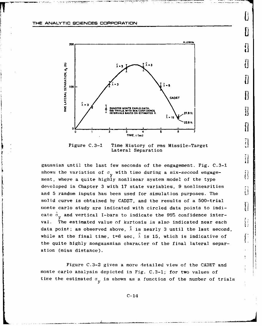
THE ANALYTIC SCIENCES CORPORATION
2W
C- 1'iC. 100-
-l
<,- CA D ET
DENOTES MONTE CARLO DATA,.S 5 D00 TRIALS. WITH 95% CONFIDENCE,
INTERVALS BASXD ON ESTIMATEDA .•,15
S22.9 ft
123 4 5 6 kTIME, t (c)-
Figure C.3-1 Time History of rms Missile-TargetLateral Separation *iI
gaussian until the last few seconds of the engagement. Fig. C.3-1
shows the variation of o with time during a six-second engage- TI
ment, where a quite highly nonlinear system model of the type
developed in Chapter 3 with 17 state variables, 9 nonlinearities
and 5 random inputs has been used for simulation purposes. The
solid curve is obtained by CADET, and the results of a 500-trial
monte carlo study are indicated with circled data points to indi-
cate a and vertical I-bars to indicate the 95% confidence inter-Y
val. The estimated value of kurtosis is also indicated near each
data point; as observed above, A is nearly 3 until the last second,
while at the final time, t=6 sec, X is 15, which is indicative of
the quite highly nongaussian character of the final lateral separ-
ation (miss distance).
Figure C.3-2 gives a more detailed view of the CADET and
monte carlo analysis depicted in Fig. C.3-1; for two values of
time the estimated a is shown as a function of the number of trials
Y
' C-14

ITHE ANALYTIC SCIENCES CORPORATION
2CZ
! '
100CADET 144.A, 95% CONFIDENCE SAND, 3
o50-
I-u-LI-
LU
I I I0' i 0 100 200 300 400 Soo
NUMBER OF MONTE CARLO TRIALS, q
R-12846'" ~40
,
' jf 30
" • CADET 022.92ft 0 0 0
LU 20- O Q
95% CONFIDENCE BAND+ , '.4
Uj 10,
100 200 300 400 500NUMBER OF MONTE CARLO TRIALS, q
1b) t - 6 saec
Figure C.3-2 Comparison of CADET and Monte Carlorms Lateral Separation
C-15
4 1

THE ANALYTIC SCIENCES CORPORATION
iiperformed, q. We note in Fig. C.3-2a that the estimated value of
G at t=4 appears to "settle" to about 145 ft after a few hundredytrials; after 500 trials we have the result that
Prob [138 ft < oy(4) < 156 ft] = 0.95 (C.3-1)
which indicates that the monte carlo estimate of a has nearly
converged to its true value with high probability. The situation
at six seconds is quite different, as demonstrated in Fig. C.3-2b.
For A = 15 the result of 500 trials is
Prob [24.7 < Oy(6) < 33.9 ft] = 0.95 (Cý3-2)
which indicate a considerable margin for error in the monte carlo .2
estimate of ay, on a percentage basis.
A synopsis of a part of the data portrayed in Fig. C.3-2b
is provided in Table C.3-1, broken down into five sets of 100 trials(set 1 corresponding to the first 100 trials, set 2 including trials101 to 200, etc.). The data demonstrates that in this case the re-
sult of 100 trials is highly random -- with & (6) varying betweeny
19.72 ft and 35.88 ft; the variation exhibited by ^ is even moredramatic. We also observe that there exists a clear relation be-
AA tiA A
twen A and a ; a is small if X is small and a is large if X isy y y
large. This phenomenon is a direct result of the basic signifi-cance of kurtosis" if X is appreciably larger than 3, then the
"tails" of the density function are abnormally heavily weighted --
implying that there is an unusually high probability of the occur-
rence of very large values of the randolw variable in comparison
with a gaussian random variable having the same standard deviation.(To cite an example, given two random variables with unity vari-
ance, yl normally distributed and y2 exponentially distributed
(A = 6; Table C.2-1), the probability that 1ylj > 3 is only 0.0027,
compared with the probability of 0.0144 that >y2 > 3.) Thus the
C-16

THE ANALYTIC SCIENCES CORPORATION
TABLE C.3-1
ESTIMATED STANDARD DEVIATION AND KURTOSISFOR LATERAL SEPARATION, t - 6 sec
100-Trial A (ft)
Set Number G y (f t)
1 19.72 4
2 32.08 15
3 22.25 6
1 4 25.67 4
5 35.88 23
Aggregate* 2.7 15[ L (500 Trials) 27.78 15
i To obtain aggregated values for a and X,it is necessary to average tne coyrespondingvalues 3f variance and fourth central moment(Eqs. (C.2-2) and (C.2-3)).
F incidence of several large values of y I in the space of a few
1.trials results in a sudden jump in the estimated aOy as evident in
the vicinity of 160 and 440 trials in Fig. C.3-2b, while it is
probable that the "settling" observed during the third and fourth
sets of trials is due to the untypically benign character of these
trials (an abnormally small number of trials occurred in which
IYt is large). Table C.3-1 thus demonstrates a fundamental pro-
blem with the monte carlo method applied to nonlinear systems:Analysis based on a modest but seemingly reasonable number of
trials (say 100) may be quite inconclusive unless the value of
X is known quite accurately in advance. Thus the analyst should
be extremely cautious in assessing the reliability of monte carlo
estimated statistics, even if the estimated kurtosis is monitored.
In the preceding example, the importance of a few large values ofj ' miss distance that occur in a set of trials in characterizing the
tails of the pdf, and thus in determining the kurtosis of a non-
gaussian random variable, also demonstrates that the common
T C-17
-~~~7 _L *----xr~7' -' E--
THE ANALYTIC SCIENCES CORPORATION
practice of "discarding the pathological trials" can lead to
very misleading r(sults. I2
C.4 CONFIDENCE INTERVAL LIMIT TABLES
The confidence interval limits of an estimated standard
deviation a can be expressed as multiples of o, viz., ii
(C.4-1)aP a
where p and P are determined only by the desired degree of con-
fidence, the kurtosis of the random variable, X, and the number
of trials performed, q. These multiples, p and p, have the form .
p 1 -*-
+7 n,, /"_qJ
(C.4-2)- 1
1 - n
where n is determined by the confidence p expressed as a decimal
fraction,
1 n 1 2-I exp (- • )dt - (C.4-3)/2- -n•
This formulation, Eq. (C.4-1), makes it particularly convenient.
to present the confidence interval multipliers in tabular form.
Thus we include Tables C.4-1 to C.4-3 for easy reference, giving
C-18

THE ANALYTIC SCIENCES COPWDORATION
3' confidence interval multipliers p and • for 90% confidence (0 -
0.90), 95% confidence and 99% confidence. This data is directly
applicable to gaussian variables, or any other case where A - 3;
for other values of kurtosis, the confidence interval multipliers
can be determined by use of the gaussian equivalent number of
trials, derived as follows: for a specified degree of confidence
(or, equivalently, a given value of n.) the multipliers p and
(Eq. (C.4-2)) are determined solely by the ratio (A - 1)/q. Thus
given a set of monte carlo trials typified by the parameters (q,X), the confidence interval multipliers are identical to those
for (q 3) whqre q is chosen to satisfyeq' eq
3 - 1 A. - 1. (C.4-4)
qeq q
or
eq - (C.4-5)
IIAV The desiied multi-liers p and p may ther be obtained from the
approprikte table of con T.4 dence interval ',,ultlpliers for gaussian
L, random v&riables under qeq"
Examile: Tr the preceding section we discussed a study of 506
trials where X - 15; to obtai" p aud T use
1000Sq~~eq •I
as given in Eq. (C.4-5). From Table C.4-2, umder the entry for 70
1 trials, we see that the 95% confidence interval limit multipliers
are p - 0.866, - - 1.225.
! 1> C -19 I
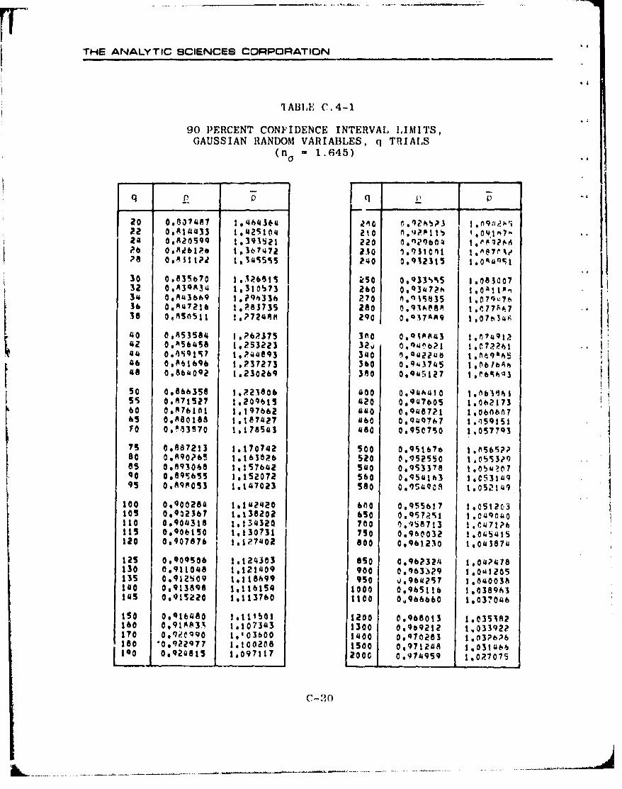
THE ANALYTIC SCIENCES CORPORATION
'IABLEY C.4-1
90 P)ERCENT CONF~IDENCE INTERVAL LIMITS,GAUSSIAN RANDOM VARIABLES, q TRIALS
(n0 1.645)
20 040074487 1.446443644 1'0 11QP3? 02.8144433 1 !:25 1I 20 tj;f~
?8 O.811t?2 1614d55i5 240 003~2315 10as
34 o8M3669 1,?96336 270 11163 .07'bu736 0.8447216 1.283735 280 0.93A6e88PAý
Is OAn5I l?748290 0q*Q7A89 1,076~34A
40 OIRS35I4 Ilpp? S 3 0.QJk#143 .414Z 0,85651 1,?25322 32v 0olnu~bpl UIiiI20.8OI61696 16237273 0 06Q75 16lb
48 0,864409a 1.230269 0 09417 jeq0
s0 0.866358 1.221806 4400 o0q44Aguo Imi51 OM757 4296S420 00947605 1.Oe217360 00876161 16197662 ago 0,9448721 1,060667
65s 0.880165 111874427 '460 00944767 l.159151
75 0.887213 181707442 So0 0,9st676 1,05657?80 0.890?65 16161626 520 00952550 1,05530985 0.893068 141576442 5~40 0,953378 l.0544?07g0 0,89S655 16152072 560 0.95441h3 18C53144995 0.89A053 1,1'47023 580 0.,7544Q0. 105214~9
100 0.9002844 IoIU24420 600 00955617 1.0St2c3105 00~02367 1.138202 650 0.9572S1 1.04"640110 0.904318 1,1344324 700 10958713 1.6447116115 0.906150 1.130131 750 0.960032 1.0t'ous5120 0,907876 1$1274402 600 09961230 1,0's38744
125 0.909506 1,124303 850 0.96?3244 1,04P?478130 0.911048 1.1~12409 900 0.963.%29 1,0442205135 0.912S09 t.118699 950 Q,964?57 1,0'b00391440 0,913898 191161S4 1000 0.965116 1,0389631445 0.915220 16113760 1100 0,966660 1.0370446
ISO 0.9164480 1,111501 1200 0.968013 1,035182160 0.91AS31 let073'43 1300 0.969212 1103392?170 019?09 90 1,403600 14400 0,970283 10PP180 100922977 1.100208 1500 0.9712448 1.0314466too 0,924481S 1.097117 2000 0.97449S9 1.027075
c ~0

STH E ANALYTIC SCIENCES CORPORATION
j 1. TABLE C.4-2
95 PERCENT CONFIDENCE INTERVAL LIMITS,GAUSSIAN RANDOM VARIABLES, q TRIALS
(n0 - 1.960)
•q £ - q £ -
20 0.7A1948 t.A'wja 100 0,914210 1.115S86P2 nA•49172 l5osqnp ItO 0016033 11Uli99
?4 ,7401 'rlgal220 0.917740 1,109165?6 0600poga 1,4q?979 230 0,919302 191064S3?a 0007596 1,464009 240 0,92050 1,103840
30 Ot?92a 1.o435490 2S0 0.922274 1610140232 0IOA?7 l141156 160 0,9236k0 1,09912130 0.821299 1.390109 IT0 00924896 1,09696236 0,M6n 1,371643 280 0,926107 1,09497038 0,828832 10359420 290 009272s9 1,093076
40 fl. 0p??3 I'langly 300 0.9263%8 1,0912A312 00935400 1,3278qS 320 0.930007 1,00798044 06836346 1.316127 340 0.932284 , 1,0899946 0dttog 1.309430 360 00934012 1.08229348 0,A03856 1029s6s 380 0.935610 190790pa
so 0,846373 1.286683 400 0.937094 10O7?SS755 0.85123 1,267136 620 0,938476 1,075S1360 0.657222 10250839 40 0,939769 1.0735276. 0,861789 1,236999 460 0.940960 1,07172970 066,i9tt 10225069 480 0.901120 1,0700S3
7S 0.669659 12184659 5S0 0,943193 1.06846580 0873087 1,205•78 SRO 0.944208 1°06701685 .876240 1.197306 50 0.945169 1106563490 0,079153 1,919940 560 0,946080 1,06433395 00861857 1#183362 S0o 0,96946 1.063104
100 0,864375 1,177346 600 0.947770 1,061940
10S 0.686729 1.171836 650 0,949670 16059286t110 0.8•936 10166813 700 0,951372 1t056938
115 0,491011 16162165 7S0 0,952908 1,050843120 0,892967 1.1S7863 600 0,95305 1,052958
12S 0,594815 1,15366? 650o O9sSqet 1,os1251130 0,896566 1,1501E3 900 O09s67?s 1,06969613S 009822? 1.186662 950 0.95837 1,044271140 0,899606 1,143400 1000 0o956840 1,o46960145 00901309 1,140335 1100 0696068# t,048624
ISO 0,902704 1.137445 1200 0.962229 1,042600160 0190542S 1,132145 1300 0,963632 19040823170 0.907o6S 1,127385 1800 0,964887 1,039248too8 Oq0*10S4 1412306! tSO0 009660t0 10037800190 0,91•226 19119167 200 0,990373 lo032517
C-21

THE ANAL YTIC BCIENLEB CORPORA7Y IN
99 PERCENT CONFIDENCE INTERVAL IAMITS,GAUSSIAN RANDOM VARIABLIES, q TRIAL.S
(n. 2.576)
pa 0.73PO71 4 6~7131 2110 I.A140'~7 111A?2 0074610"t P.208IM9 ec .032 1 0pI241 0.7i3870 ?,(13941I7 220 0,A95.306 1 tb 126 0.7b(~6' 9,9193#09 230 0'"97lbs 114hl
30 0,777334i 117SM631 250 60.01358 1.141'Q3632 ý9777496 to700693 ah 2,0310I0l1
34 07APP71 1,653232 270 * V)904S~m ,~i3IMP~716 0.7iAhC9 11613199 280 )l9otboba 140"91IS 017;08d9 14578906 290 019074A67 14106'109
M0 OvTQ472S 1*495 300 neq06A3u0 is245ý412 067,08365 1,5230418 320 00911370 l.1?0ol
O.60001794 10490936 3410 0.913"90 eitl416 0.605031l 1,4179303 360 0091SA3O ,1ph
53 ,A7h~ 1401914 0.O921371 161029'4s60 09823597 1,5791414 4140 0.??979 1.10fl204165s 0,a82928 1.355002 4160 0.9241488 1,097h6270 0.631757 1034'56S 4180 60295409 1,095298
75 0.83R160 1.31,003 5a0 0,927249 W.9309180 0.Rg?19q 1*301717 520 0.928517 1009102a1A5 6,A49,922 1.288269 5410 09924718 1,089085g0 0.M419371 10?76330 560 0.,'30e8s 10C672A095, OI65P579 192656MM Sa0 0.931942 loli?
100 0.8ssi72 1.256012 600 0.932976 1,083913105 0.656376 l.2417278 650 0,935359 1.0610208110 0.661009 1,239313 700 0*137498 :00 7&Q'4 0115 0,A63489 1.2320144 750 0.9394131 1.0741030120 0.86503l 1.225295 S00 0.9411191 1,0714118
125 0.6680417 1.210087 850 0,9412801 1.069057130 00870118 1*?13S26 g00 0,9u"'282 11064i909135 010721415 1,207969 950 09941q6SI 1,064194151410 008741046 10202966 1000 0.9416920 1,0631391415 09475858 1,190283 1100 0,9419208 1.059929
ISO 0,877S49 1.193888 1200 0.951216 1.05712160 0.880630 11168556 1300 0,952999 1,052L720170 00AM3410 1.178686 14100 019SiU595 1,052569IS0 0.086363 1.172236 1500 00956,35 1,0506417190 0.689118 101664102 2000 0.9615941 1,0413410
C-22

y THE ANALYTIC S.IENCES COFVMO:ATION1;
L.
* REFERENCES
1. Gelb, A. and Warren, R.S., "Direct Statistical Analysisof Nonlinear Systems: CADET," AIAA Journal, Vol. 11,
,V No. 5, May 1973, pp.689-694.
2. Price, C.F. and Warren, R.S., "Performance Evaluation ofHoming Guidance Laws for Tactical Missiles," The AnalyticSciences Corp., Report No. TR-170-4, January 1973.
3. Warren, R.S. and Siegel, J., "Htissile Performance AnalysisUsing CADET," The Analytic Sciences Corp., Report No.TR-286-2, August 1973.
4. Taylor, J.H. and Price, C.F., "Direct Statistical Analysisof Missile Guidance Systems via CADETTM," The AnalyticSciences Corp., Report No. TR-385-3, to be published.
5. Jazwinski, A.H., Stochastic Processes and FilteringThaory, Academic Press Inc., Few York. 1970.
6. Gelb, A. and Vander Veldo, W.E., Multiple-Ineut Describ-ing Functions and Nonlinear 3ystem Desirn, McGraw-HillBook Co., New York, 1968.
7. Phaneuf, R.J., "Approximate Nonlinear Estimation," Ph.D.Thesis, Dept. of Aeronautics and Astronautics, M.I.T.,Cambridge, Mass., May 1968.
8. Papoulis, A., Probability, Random Variables, and Sto-chastic Processes, McGraw-Hill Book Co., New York, 1965.
9. Price, C.F., "Optimal Stochastic fuidance Laws forTactical Missiles," The Analytic iences Corp.,Report No. TR-170-2, Septimber 1.
10. Price, C.F., "Adaptive Control and Guidance forTactical Missiles," The Analytic Sciences Corp.,Report No. TR-170-1, Vol. II, June 1970.
11. Gelb, A. (Ed.), Ap lied Otimal Estimation, The MITPress, Cambridge, Mass., 1974.
"12. Bryson, A.E., Jr. and Ho, Y.C., Applied Otimal Con-trol, Blaisdell Publishing Co., Waltha, Mass., "1969.
R-1
THE ANALYTIC SCIENCES CORPORATION
13. Willems, G., "Optimal Controllers for Homing Missiles,"Report No. RE-TR-68-15, U.S. Army Missile Command, iRedstone Arsenal, Huntsville, Alabama, September 1968.
14. Skolnik, M.I., Introduction to Radar Systems, McGraw-HillBook Co., New York, 1962.
15. Gibson, J.E., Nonlinear Automatic Control, McGraw-HillBook Co., New York, 1963.
16. Goldstein, H., Classical Mechanics, Addison-WesleyPublishing Co., Reading, Mass., 1950.
17. Gradshteyn, I.S. and Ryzhik, I.M., Table of Integrals,Series, and Products, Academic Press Inc., New York, 1965.
18. Abramowitz, M. and Stegun, I.A. (Eds.), Handbook ofMathematical Functions with Formulas, Graphs, and Mathe-matical Tables, No. 55 in National Bureau of StandardsApplied Mathematics Series, U.S. Department of Commerce,Washington, D.C., 1964.
19. Peirce, B.O. and Foster, R.M., A Short Table of Integrals(Fourth Ed.), Oxford University Press, London, 1956.
20. Geier, J,G., "Approximate Direct Statistical tnalysis ofNonlinear Systems," Master's Thesis, Dept. of Aeronauticsand Astronautics, M.I.T., Cambridge, Mass., June 1973. A
21. Bucy, R.S., Hecht, C. and Senne, K.D., "An Engineer'sGuide to Building Nonlinear Filters," Seiler ResearchLab. Report No SRL-TR-72-0004 (USAF Systems Command),May 1972.
22. Bowker, A.H. and Lieberman, G.J., Engineering Statistics,-.Prentice-Hall, Inc., Englewood Cliffs, N.J., 1959.
23. Siegel, J., "Missile Performanc3 Analysis Using CADET,"The Analytic Sciences Corp., Report No. TR-449-1, to [Jbe published.
R-2