AD-A±24 883 DIGITAL ESTIMATION AND CONTROL FOR AIR REFUELING /RENDEZVOUSCU) AIR FORCE INST OF TECH IRIGHT-PATTERSONAFB ON SCHOOL OF ENGINEERING J T RI YARD DEC 82

UNCLASSIFIED AFIT/GA/EE/82D-i .F/G L2/1i M

.)

lu1j32 IL

II- IfLO

1.25* 1111. 1 116

" MICROCOPY RESOLUTION TEST CHART

,

NATIONAL BUEUOF STANDARDS -I963-A "

40.

II --

uuiii I.

U. -UI** I.

11111- It

• o"III • -

OFF

DIGITAL ESTIMATION AND CONTROL FOR

AIR REFUFrlING RENDEZVOUS

THESIS

AFIT/GA/EE/8_D-1 James T. RivardCapt USAF DTIC

LI-J ( ELECTEFA 24 1983

C.*DEPARTMENT OF THE AIR FORCE EAIR UNIVERSITY (ATC)

AIR FORCE INSTITUTE OF TECHNOLOGY

Wright-Patterson Ai, -rce Base, Ohio*

LI ' r "

"pr O

A

AFIT/GA/EE/82D-1

DIGITAL ESTIMATION AND CONTROL FOR

AIR REFUELING RENDEZVOUS

THESIS

AFIT/GA/EE/82D-1 James T. RivardCapt USAF

Approved for public release; distribution unlimited

i'a

AFIT/GA/EE/8 2D-1

DIGITAL ESTIMATION AND CONTROL FOR

AIR REFUELING RENDEZVOUS

THESIS

Presented to the Faculty of the School of Engineering

of the Air Force Institute of Technology

Air University

in Partial Fulfillment of the

Requirements for the Degree of

Master of Science

SAccession For

Cc,. . .

4 -for

by

James T. Rivard,B.S.'Capt USAF

Graduate Astronautical Engineering

December 1982

Approved for public release; distribution unlimited

Preface

In 1980, the C-141B modification program began in earnest.

Suddenly, C-141 flight crews had to develop expertise in an area

in which they had virtually no experience - air refueling. The

difficulties which many, including myself, encountered, prompted

this research. Above all, this study's goal is simply to make

things easier for the crewmember, who is given a variety of

missions and limited training resources. Hopefully, this paper

will cause others to look more closely at the air refueling

problem in order to develop simpler, more efficient methods.

I am indebted to many people for their help in this

effort. I am especially grateful to Lt Col Edwards for all of

his advice, guidance, and patience. I would also like to

thank all of those who assisted in the research, particularly

Lt Ham and Greg Santaromita at Wright-Patterson, Maurice Johns

with Delco, and Bob Harper at Collins. And, I am grateful that

the typist, Linda Kankey, can meet a deadline better than I can.

James T. Rivard

ii

r-. -Contents

Page

Preface. . . . . . . . . . . . . . . ii

List of Figures . . . . v

List of Tables . . . . . . . . . . ..... vi

,'-Abstract . . . . . . . . . . . . . . . . . . . . . . . . . vii

SI. Introduction .1

II. Air Refueling Rendezvous. . . . . . . . . . . . . . 4

Rendezvous Problem .*............. 4Present Method . . . . . . . . . . . . .... 6Proposed Method 7

III. Truth Model . . . . . . . . 9

Coordinate System . . . . ........... 9Receiver Dynamics . . . . . . . . . . . . . . . 10Cross-track Error . . w * . . .. . .. . .. . 12Along-track Error . . . . . . . . . . . . .. 17Altitude Separation . . . . . . . . . . . . . . 20TACAN Error . . . . . . . . . . . 22Summary . . . . . . . . . . . . . . . . . . . . 23

IV. Estimation . . . . . . . . . .. 28

Extended Kalman Filter ............. 28Dynamics Model .... . . . . . . . . . 31Measurement Model . . . . . . . . . . . . . . . 35Initialization . . .. .. . . . . . . . . 35Propagation . . . . . . . . 0 . . 0 . .. . .. 39Update . . . . . . . . . . . . . . . . . . . . 40Estimation Algorithm. . . . . . . ....... 42

V. Control . . . . . . . . . . . . . . . . . . . . . . 45

Tanker Dynamics . . . . ............ 45Turn Point . . . . . . . . . . . . . . 47Closed Loop Control .............. 53

VI. Simulation Results . . . . . . . . . . . . . . . . 57

Simulation. . . . . . . . . . . . . . . . . . . 57Filterl e. . . . . . . . . . . . . . . . . . . 58Controller . . . . . . . . . . .. 69

iii

Contents

Page

VII. Conclusions . . . . . . . . . ** ***** * 77

VIII. Recommendations . . . . a . . . . . . 79

References . . . . . . . . . . . . . . . . . . . . . . . . 81

iv

List of Figures

Figure Page

1 Point Parallel Rendezvous . . . . . . .... 5

2 Coordinate System ........... . . . .. 10

3 Tanker Free Body Diagram (Tail-on view) 48

4 Rendezvous Turn Geometry .............. 48

5 Standard Deviation of ^ Error for Non-Radar-AidedRendezvous . . . . . . . . . . . . . . . . . . .. . 60

6 Actual and Predicted x Estimate Error Statistics. . 63

7 Actual and Predicted vxe Estimate Error Statistics. 64

8 Actual and Predicted y Estimate Error Statistics. . 65

9 x Estimate Error Statistics-2 Sec Sample Period . . 66

10 v Estimate Error Statistics-2 Sec Sample Period . 67xe

11 y Estimate Error Statistics-2 Sec Sample Period . . 68

12 y Estimate Error Statistics - No TACAN Bias Error. 70

13 Effect of Control Gain on RMS Miss Distances. 74

v

"oa

List of' Tables

Table P age

*1 Rollout Error Statistics . . . . . . . . . . . . . . . 72

2 Rollout Error Statistics -Turn Initiated From Other

Than Nominal Conditions . . . . . . . . . . . . . . . 75

vi

AFIT/GA/EE/82D-1

Abstract

Estimation and control algorithms were developed for

use by a tanker aircraft conducting an air refueling rendezvous.

A stochostic model of a typical rendezvous was developed first.

Then an entended Kalman filter which uses air-to-air TACAN

distance measurements was designed. Also, algorithms were

derived for computing the tanker's appropriate offset, turn

point, and closed loop bank angle commands during the final

turn of a point-parallel rendezvous,-

In Monte Carlo simulations, a 3 state extended Kalman

filter provided a stable, though limited, means of estimating

the receiver's position and velocity throughout the rendezvous.

Also, the control algorithms exhibited two advantages over the

present rendezvous method: turn point solutions could be computed

for other than nominal offsets and headings, and bank angle

commands during the turn reduced position errors at rendezvous

completion. When compared to the present method, root mean

square, cross-track distance errors at rollout were reduced as

much as 75%, and along-track errors were reduced up to 47%.

vii

DIGITAL ESTIMATION AND CONTROL

FOR AIR REFUELING RENDEZVOUS

I Introduction

Certainly, in-flight refueling is a vital element of Air

Force strategy and tactics. It has long been a critical part of

bomber and fighter operations. Recently it has assumed an

increasingly important role in airlift planning as well, parti-

cularly with the advent of the Rapid Deployment Force. The Air

Force's large fleet of KC-135 and KC-10 aircraft provide the

United States with a unique military capability. No other nation

in the world can project, in a matter of hours, such a wide range

of military responses to a perceived threat anywhere in the world.

Of course the great advantage of in-flight refueling is

that it eliminates the need for enroute airfields. Many naviga-

tional systems have been designed to get an aircraft safely into

an airfield. However, there are no systems in operational use

designed specifically for conducting air refueling rendezvous.

Instead, a wide variety of navigation and radar systems designed

primarily for other purposes are adapted to the problem. The two

aircraft usually get together, but the initial rendezvous attempt

is often very inaccurate. That frequently causes excessive

maneuvering and delays in completing the join-up. Those undesir-

able effects take on additional significance for large aircraft

requiring extended refueling time, aircraft formations, and

refueling operations at night or in instrument weather conditions.

- 1

Hardware technology exists which should meet any practical

rendezvous specification. The first step in upgrading our air

* - refueling systems, though, is to investigate what improvements

can be made with the existing equipment.

The KC-135 fleet was recently equipped with an inertial

navigation system (INS). An integral part of the INS is the

navigation computer. This computer uses information from the

inertial instruments and the central air data computer (CADC) to

* compute aircraft position and velocity, and wind information.

It also calculates steering commands for the autopilot and flight

director system. The KC-135 and all Air Force refuelable aircraft

are also equipped with Air-to-Air TACAN (Tactical Air Navigation).

The system provides a measurement of straight line distance to

other TACAN equipped aircraft.

A possible system improvement would be for the tanker to

use TACAN measurements as inputs to an estimation algorithm which

has outputs of the other aircraft's position and velocity. These

estimates would then be used to compute steering commands for the

tanker during the final part of the rendezvous. If all of those

4 estimation and guidance computations can be handled by the present

onboard navigation computer, the system could be implemented

entirely on current hardware.

id The purposes of this study are to develop an estimation

and control method for solving the rendezvous problem and to see

what improvements in accuracy such a system might achieve.

2

n -rr-

Along with the existing hardware constraint, operational feasi-

bility is a prime consideration throughout. The standard

rendezvous profile is altered as little as possible so that

present methods can always be used as a back-up.

', .

.

4

p3

4d

II Air Refueling Rendezvous

The most common type of rendezvous is called the point

parallel rendezvous. In this type, the tanker waits for the

receiver, the aircraft to be refueled, at a planned point along

the receiver's route of flight. The rendezvous is accomplished

and the refueling completed on a refueling track in the receiver's

general direction of flight. This type of rendezvous will be

discussed here.

Rendezvous Problem

A typical point parallel rendezvous is depicted in Figure

1. The tanker waits at refueling altitude in a holding pattern

at the control point (CP). When the receiver reports that he has

passed the initial point (IP), the tanker departs the holding

pattern and flies towards the receiver. Meanwhile, the receiver

proceeds along the refueling track at constant airspeed and

descends to an altitude 1000 feet below the tanker. The tanker

attempts to establish the correct offset and turn at the right

time so as to roll out of a 30 degree bank turn two nautical

miles directly in front of the receiver. The receiver then

closes to one mile from which point the rendezvous is completed

visually.

The rendezvous problems for the tanker, then, are to

compute and fly the appropriate offset, turn at the correct time,

and maintain proper bank angle throughout the turn.

444

II

?Initial Point

,U I

30 Bank Turn

Receiver f

2NM u n o tOffset Turnpoint

Tanker.

* "Control Point

Figure 1 Point Parallel RendezvousI5

; ., 5

0".I

Present Method

Currently, a chart is used to determine the correct offset

and turn point. Given values for receiver true airspeed and

drift angle, the chart gives the appropriate offset and distance

from the receiver to initiate a 30 degree bank turn. Here, drift

angle, the number of degrees the aircraft must crab into the wind

to maintain a course parallel to the refueling track, is used as

a measure of the wind component perpindicualr to the track.

Since the tanker and receiver navigation systems do not agree

exactly, they attempt to establish the desired offset by observing

the other aircraft's position on radar. When the tanker's TACAN

and/or radar indicates the receiver is at the calculated turn

range, the tanker rolls into a 30 degree bank turn which he holds

antil he has turned to the refueling heading.

The present method has several inaccuracies. The offset

and turn range chart only gives distances to the nearest mile;

fluctuations in wind or airspeed are not compensated for; equipped

with a radar designed primarily for weather, it is difficult for

the KC-135 to determine accurately another aircraft's position;

and, finally, the system is entirely open loop: a constant 30

degrees of bank is held throughout the turn. Even under the

best visual conditions it is difficult for either the tanker

or receiver to recognize any need for corrections until the turn

is nearly complete.

6

a

Proposed Method

The proposed method would be basically the same proce-

dure but with two improvements. Rather than using a chart, the

correct offset and turn point would be calculated and periodically

updated by the navigation computer. Also, an estimation algorithm

using Air-to-Air TACAN distance measurements would be used to

estimate continuously the receiver's position and velocity.

UThat estimate would be used as input to a closed loop digital

control algorithm before and during the turn.

A rendezvous conducted with such a system might proceed

as follows:

1. Rendezvous data is loaded into tanker's INS

anytime prior to rendezvous. Data includes

control point coordinates, refueling track

heading and altitude, and receiver altitude

and airspeed.

2. Using these input data and information from the

tanker's INS and central air data computer,

the navigation computer calculates and displays

.4 the appropriate offset.

3. Tanker and receiver attempt to establish correct

offset using radar.

14 4. Estimator is initialized based on planned

receiver track, altitude, and airspeed, and

computed wind velocity. A manual radar update

might also be used.

"' 7

4

I

5. Estimation algorithm propagates receiver state

estimate and uses TACAN measurements for updates.

6. Computer calculates and displays time until turn

and commands a turn at updated turn point.

7. Digital controller provides bank angle commands

to the autopilot/flight director to reduce error

at rollout.

The first step in designing such a system is to create

a mathematical model of the rendezvous procedure just described.

That model will later be used as the starting point for the

estimator design, and as a reference or truth model for computer

simulations.

8

i'8

III Truth Model

Research was conducted into present air refueling proce-

dures, the KC-135 inertial navigation system, TACAN systems,

and wind models. The result, as developed in this section, is

a stochastic state differential equation and measurement equation

which hopefully describe the actual dynamics, uncertainties, and

errors reasonably well. For different types of receiver aircraft,

the form of the state equations will be the same. However, there

will be slight variations in certain parameters and error statis-

tics due to different rendezvous airspeeds and navigation equip-

ment. In the truth model development and the simulations, a

standard rendezvous with a C-141 is modelled. This study, while

limited to one aircraft type, should indicate both the practical-

ity and the potential benefit of the proposed system.

Coordinate System

The coordinate system for the truth model is depicted

in Figure 2. It is a simple, two-dimensional, rectangular

system parallel to the tanker's local horizon plane. The origin

is located at the control point (CP) at refueling altitude. The

plus x axis points towards the initial point (IP), and the plus

y axis is oriented as shown. Aircraft headings, T, are measured

counter-clockwise from the plus x axis.

9

. ..- .. 4 lum m " mL ul u m~

IP

L mx

CPy I

Figure 2. Coordinate System

The exact reference frame location and orientation are defined

by the INS, so the frame varies slightly from a true ground

0 fixed system due to INS errors. The advantage of defining the

system by the INS is that INS tanker position readouts are

deterministic rather than random variables.

Rectangular coordinates are chosen to make the filter

state propagation equations linear. Also, this particular axes

orientation simplifies turn point calculations: y position

coordinates determine offset, and x position and velocity com-

ponents determine the time to turn.

Receiver Dynamics

4 For an aircraft, the velocity in a ground fixed frame is

found from

v =v a/w +(1)

10

where v is velocity relative to the ground, _va/w is velocity of

the aircraft relative to the wind or air mass, and v is the

* velocity of the wind.

. The receiver attempts to fly a ground track along the

x axis. In order to do so, he must apply a drift correction, 6,

into the wind such that the y component of velocity, vy, is zero.

Since he is heading in the -x direction, his heading will then

be '=w + 6.

The receiver pilot will also attempt to maintain a

preplanned indicated airspeed. The tanker can convert this

indicated airspeed to an equivalent true airspeed, vR, based on

rendezvous altitude and measured air temperature. The components

of Va/w are then

Va/w x v ccs (i + S)

and

va/w y VR sin (r + )

or, equivalently,

va/w x = -vR cos

and

Va/w y -vR sin 6

If the receiver maintains v = 0, the y component of Eq(1)

*becomes

0 = -vR sin 6 + vR wy

which can be used to find 6.

4 11

I . ,._ m, . . ... ,, ,, ,.,...: . a,,=l, ,n,, ,wt.--: ,.- , l ~ d ~ , m ,N m

, 2The navigation computer continuously calculates the wind vector,

w , by subtracting Va/w- determined from measured true airspeed

and aircraft heading - from the INS computed velocity, v. The

planned refueling track heading can then be used to calculate

Vwx and vwy.I.! Now the velocity relations for the receiver can be

written. The receiver attempts to fly such that

= sin vwy (2)

v R"

Vy 0

and

v = -vR cos6 + Vwx (3)

r Of course his flight will not exactly satisfy those equations.

Instead, the actual velocity relations will be

v vy ye

and

v= -vR cos 6 + v + v.wx xe

where v xe and v ye are the velocity error components.

Cross-Track Error

As mentioned previously, the modelling parameters in

this study are based on a standard rendezvous of a KC-135 and a

C-141. Both aircraft are equipped with a Carousel IV inertial

navigation system made by Delco. The C-141's autopilot can very112

accurately maintain the course computed by its INS. The INS,

though, drifts slightly during flight and is the source of some

cross-track error.

Data from several hundred military and commercial flights

indicated a 95% confidence figure of 1.65 NM/hr for the Carousel

IV INS. According to Delco, a 95% cross-track confidence value

can then be estimated as 66% x 1.65 NM/hr = 1.1 NM/hr (Ref 1: 6-1).

Using this as a 2a value, the INS has a la cross-track error rate

of 0.55 NM/hr.

Position errors in an INS have a variety of sources and

the associated error models can be very elaborate (Ref 2).

However, for the short time interval of a rendezvous - less than

10 minutes, the cross-track error might be reasonably modelled

U as the sum of a constant rate component and a small random alk

component. Because the rendezvous duration is brief compared

to the 84 minute Schuler period, and because this study is for

feasibility and not detailed operational design, second-order,

coupled error models are not included.

The random constant error rate, v models the long term

position error source which flight tests have shown to be the

dominant source of velocity error for the Carousel IV (Ref 1: 6-6).

v yc is assumed to be Gaussian and zero mean, and to have a standard

*g deviation of 0.55 NM/hr. It is also assumed to be stationary:

the error rate over a short period has the same statistics as

the error rate over the whole flight. But that is only the

error rate due to the receiver's INS. Remember that the receiver's

13

0

position and velocity are estimated in the reference frame of

the tanker's INS. Any error in the tanker's INS is then perceived

as an error in the receiver's state. So the total, apparent,

constant drift rate is

- vVyc yc Receiver yc Tanker

Since each INS operates independently, and the two aircraft may

fly entirely different routes to the rendezvous, their random

drift rates are assumed to be independent. Then vyc is zero

mean, Gaussian, and

2 2 2

avyc = Cvyc Receiver + avyc Tanker

a vy c is thus calculated to be 0.778 NM/hr.

A random walk component of position error, y w is added

to account for small deviations from the simplistic, constant

error rate model. This component is modelled by

Yw(t) = w y(t)

where w (t) is a zero mean, continuous, white noise, andyE{w (t) Wy (t+T)} = qy6(T)

y

E{-} is the expected value operator, 6(-) is the Dirac delta

function, and qy is called the strength of the white noise.

This type of model results in a zero mean process with2

E (yw (t)} = qy (t-to )w y 0

where t is the initial time of the simulation.I-

14

. --

Choosing an appropriate value for q was somewhat

arbitrary. Schuler oscillations contribute a 0.2 NM/hr CEP

velocity error component (Ref 1: 6-6). Over the short 10 minute

rendezvous period, a 0.2 NM/hr error would cause a 202 ft posiLion

error. To account for both aircraft's errors, INS errors for

which no error data could be found, and autopilot errors, a la

value for y at the end of a 10 minute period was chosen to beYw

500 ft. The idea here was to choose a conservative (high) value

for the magnitude of the errors not modelled by vyc. Since the

proposed method would have to be suitable for several receiver

aircraft types, a specific C-141 INS error model is inappropriate.

The noise strength is then found to be2

(500 ft) 2

q ( 25000 ft /minQ7" (10 mai)

5 2

1.13 x 10- NM /sec

The model for cross-track position and velocity is now

written as

= v (t)ye

vye(t) = Vyc + WY(t)

4E{v } = 0, a = 2.161 x 10 NM/secyc vyc

5 2

Ew y(t)} = qy = 1.13 x 10- NM /sec

15a-

Now, only the initial condition statistics for y(t) remain

to be specified. In the simulations, two different situations

are modelled. In one case, the rendezvous is conducted without

the assistance of radar and each aircraft is navigating solely

off of its unaided INS. Assuming the two aircraft's INS errors

are independent, Gaussian, zero mean, and have a la error rate

of 0.55 NM/hr, y(O) is also zero mean, Gaussian with

a 20 (0-55 )2 + (0-55 ta 2

yo aR aT

Here tR and taT are the airborne times, in hours, of the receiver

and tanker. For an airborne time of 10 hours for the C-141 and

5 hours for the KC-135, a is computed to by 6.15 NM. Ofyo

course this much total error would be extreme. Normally, one

or both aircraft would have the opportunity to update its INS

somewhere enroute, or the rendezvous track may be defined by

radio navigation aids. This "worst case" is included to get a

feel for the limitations, if any, of the proposed system.

The case in which radar is used to help estimate the

receiver's position is also modelled. In this case

E{y(O)} = YT(O) +

where YT is the tanker's y coordinate and A^o is a manually

inserted estimate of the lateral distance between the two

aircraft. The accuracy of this estimate varies with range.

Error due to radar azimuth misalignment decreases linearly with

4I range. Also, at shorter ranges the radar display can be set to

16

4o

-4,

a smaller scale. No data on the accuracy of such an estimate

could be found, so a a value was assumed. From personalyo

experience, it seemed reasonable to say that a crewmember can

estimate bearing from a radar display to a la accuracy of 2

degrees. At 60 NM range, a 1 degree azimuth error results in

about a 1 NM cross-track error. The relationship between azimuth

and cross-track error is nearly linear, so a la azimuth error

is assumed to cause a ayo value of 2 NM for a 60 NM radar range,

and a ayo value of 1 NM for a 30 NM radar range.

Along-Track Error

The receiver's along-track position and velocity

components are modelled by

x = v

x -vR cos + vwx + vxe (4)

The tanker can convert the receiver's planned indicated

airspeed to the true rendezvous airspeed, vR, using altitude

and air temperature data from its central air data computer (CADC).

INS and CADC data can also be combined to compute the wind velocity

conponents, vwx and vwy. Using Eq(2), 6 is then calculated.

These estimated values for vR, 6, and v are only computed at

the start of the rendezvous and remain constant. In Eq(4), vxe

is then treated as the only random variable. vp , 5, and vwx

could be continuously updated, but then the spatial correlation

of those computed values and v xe would have to be accounted for

17

in the truth and filter models. Certainly this would be an area

for future consideration, but it was considered beyond the scope

of this study.

v in modelled as the sum of a random constant and anxe

exponentially-correlated component. The constant component is

primarily due to instrumentation and pilot bias errors. This

bias would include factors such as tanker errors in computing

the wind components, error in the receiver's displayed airspeed,

the receiver pilot's inability to maintain the correct airspeed

on average, and differences in temperature between the two

aircrafts' positions when vR is computed. To get a rough idea

of the magnitude of this bias error, the individual error

sources were assigned variances. The figures used were not

0 explicitly listed as standard deviations; approximate lo -lue

had to be surmised from published CEP values and tolerances,

computer flight plans, and personal experience. The following

la error values were used: tanker ground speed - 1 knot (Ref 1:

6-6), tanker and receiver true airspeed - 2 knots each (Ref 1:

7-5), airspeed change due to change in temperature between IP

4and CP - 1 knot (Ref 3: 10-17, 30), and pilot error - 5 knots.

Since the total error is the sum of each of these

components, and they are each assumed to be independent, the

variance of the total error is the sum of the individual variances.

The result is a variance of 35NM 2 /hr2. The random constant

component of error, vxc, is then modelled as Gaussian, zero mean,

with a standard deviation of 6 NM/hr.

18

0

The correlated component is due mainly to wind fluctua-

tions. Wind data is difficult to interpret. The models can be

very complicated and vary considerably with the altitude and

frequency ranges considered. A basic approximation, though,

is that wind velocity is exponentially, spatially correlated

(Ref 4: 2). Aircraft ground speed is mainly affected by just

the slowly varying winds since high frequency gusts have

no net effect on aircraft displacement. An exponentially corre-

*lated wind model, with a correlation distance of 50 NM, was

adopted from ( Ref 4: 2).

In the time domain, vxf, the fluctuating component

of along-track velocity error, is modelled by the equation

1

vxf (t) -- v xf(t) + wf(t)

where Tf is the time constant, and wf(t) is a continuous white

noise process. Tf is found from the equation

T =Correlation distance

Airspeed

to be 455 sec for a C-141 traveling at 396 knots. A la value of

10 knots was chosen for vxf(t). This figure seemed reasonable

after examining forecast wind variations along refueling tracks

on actual computer generated flight plans (Ref 3: 10-17, 30).

The appropriate strength of the zero mean, white, Gaussian noise

wf(t) is found from the equation

2q2 (Ref 5: 178) (5)

T19

4

to be 3.39 x 10-8NM2/s _. The resulting vxf(t) process is zero

mean, as it should be if the wind velocity at the tanker's

position is considered the mean wind. Remember that vxf is not

the total wind, it is just the fluctuating component of

deviation from an estimated wind, vWX*

Altitude Separation

In the truth model, position and velocity components

are measured in the local-level coordinate frame discussed

earlier. However, the receiver will actually be displaced

vertically from the reference plane due to a planned altitude

separation, altimeter errors, and the curvature of the earth.

The planned altitude separation, a0 , is usually 1000i0

ft or 0.164 NM. Altimeter error, though, will cause some

0' deviation from ao , even if both aircraft are using the same

altimeter setting. When flying at a constant altitude over a

relatively short distance, the error is essentially constant

(Ref 6: 4-4). A zero mean, Gaussian random bias is then used

to model the net error. Maximum acceptable error before takeoff

is 75 feet, but the error increases slightly with altitude.

For the simulated rendezvous altitude of 25000 ft, a standard

deviation of 150 ft or 0.0247 NM is assumed (Ref 7: 1-5, 1-6).

The further away the receiver is from the tanker, the

4 more it will fall below the tanker's local-horizon reference

plane. The amount of vertical displacement is r (1 - cose

where re is the radius of the earth, and is the angle of

20

4

central arc which separates the two aircraft. The angle can be

found fromS

re

where s is the arc length between the two aircraft. For the

short distances involved - less than 100 NM, s is approximated

by d, the straight line distance between the tanker and receiver.

A value of 3444 NM is used in the simulations for re

The altitude separation model is then

a = a +a +a0 e c

where a is the total altitude separation, a is the planned0

separation, a is altimeter error, and a is vertical displace-e cment due to the curvature of the earth.

Incidentally, the velocity component v x , as viewed from

the tanker, will also be affected slightly due to the curvature

of the earth. The receiver's velocity vector is oriented out

of the horizontal plane by the angle (b described above. However,

the maximum horizontal velocity change due to this effect is

less than 0.2 NM/hr for a receiver true airspeed of 400 NM/hr.4 At the initial TACAN ranges, where this effect is the greatest,

the final estimator design only achieved a la accuracy of about

10 NM/hr, so ignoring this effect in the truth model does not

affect the simulation results.

421

TACAN Error

With air-to-air TACAN, the tanker can measure the

straight-line distance to another TACAN equipped aircraft. TACANs

can also provide a bearing measurement to TACAN ground stations,

but the KC-135's current system does not provide bearing capability

for air-to-air operation (Ref 10: 1). The TACAN error model

used in (Ref 4: 3) and (Ref 8: 18) was adopted. TACAN

measurements are modelled by the equations

dT(t) = d(t) + de(t)T e

and

d (t) = b + n(t)e

where dT is the TACAN measured distance, d the true distance,

0and de the TACAN error. The error is the sum of a random bias,

b, and a short correlation time component, n.

The KC-135 was recently equipped with an improved

system, the AN/ARN 118 (V) TACAN made by Collins. Test results

(Ref 9: 1), published tolerances (Ref 10: 9), and flight

test results of a similar system (Ref 11: 16) indicate the

model described above is reasonable, but that the standard

deviations for b and n are less than those used previously.

The bias, b, is modelled as zero mean, normally dis-

,4 tributed (Ref : 3), and having a standard deviation of 0.1 NM

(Ref 10: 9). n(t) is modelled as a zero mean, Gauss-Markov

proo.3s (Ref 4: 3) generated by the system• 1

n~t = - T n(t) + Wn(t)

n

22

0Q

F.

The correlation time, Tn , is 3.6 sec (Ref 4: 3). The standard

deviation of n, for the new TACAN, is 0.016 NM (Ref 9: 1)

(Ref 11: 16). The appropriate strength of the continuous, white

Gaussian noise process is found from Eq(5) to be 1.422 x 10-NM2 /

sec.

Summary

The entire truth model is summarized below. Random

variables are underscored with a tilde, and mean and standard

deviation values are denoted by m and a respectively. Non-

random variables, such as vR , are determined from planned rendez-

vous parameters, and INS and CADO data. The listed values are

those used in the simulations.

6 =sin-1-- (6)

6 = Drift correction

vwy = y component of wind

v R = Receiver true airspeed

vR = 0.110 NM/sec (396 NM/hr)

yc + (t) (7)

z(t) = Receiver's y coordinate

4 No radar aiding:

myo = 0y o = 6.15 NM

23

1f

With radar aiding:

my YT(0) + AA=o Y YO

where = Tanker y coordinate

Ayo = Estimated offset

ayo = 1 NM for 30 NM radar range

vyc Constant component of lateral drift

mvyc = 0, a = 2.161 x 10-NM/sec (0.778 NM/hr)vyc vyc

W(t) = Continuous white noise-y

mw 0, = 1.13 x 10- Nv,/sec= q

" (t) = -VR cos + V + V + v (t) (8)R Vwx ~XC ~xf

x(t) = Receiver x coordinate

v wx x component of wind

v = Constant component of x velocity deviation

m = 0 , = 2.78 x 10-3 NM/sec (10 NM/hr)vxc

Vxf Fluctuating component of deviation

mvxf = 0,0vxf = 1.67 x 10- 3NM/sec (6 NM/hr)

SxfCt) -- vx(t) + wf(t) (9)Tf

Tf = Correlation time

Tf = 455 sec

24

wf(t) = Continuous white noise

m = 0, qf = 3.39 x 10-ONM 2/sec 3

a = a o + a e + a c (10)

a = Altitude separation

a = Planned separation

a = 0.164 NM (1000 ft)

a =Altitude error-e

mae = 0 = 0.0274 NM (150 ft)

a Separation due to curvature of the earthC

a = r {1-cos(d/r e )c ee

r = 3444 NMe

d = Distance between aircraft

de(t) = b + n(t) (11)

d (t) = TACAN measurement error

4e-~e

4i b = TACAN bias

mb = 0, ab = 0.1 NM

n(t) = Short correlation component of error

4mn = 0, a = 0.0160 NM

n(t) - I-n(t) + wn(t) (12)Tn

25

I

T =Correlation timen

T 3.6 see

f (t) =Continuous white noise

m wn 0, q n = 1.1422 x 10- 4NM2/sec

In matrix form, the dynamics are described by

x0 1 1 0 0 0 0] X -V RCos 6+ v w

V xc 0 0 0 0 0 0 0 c 0

x 0 0 0 0 0 0 Vx 0

d y =0 0 0 0 1 0 0 y +0

dt vy 0 0 0 0 0 0 0 Vy 0

a e 0 0 0 0 0 0 0 a e0

b 0 0 0 0 0 0 0 b 0

n 0 0 0 0 0 0 -T nLL nj 0

ro 0 0

:4 0 0 01

Ii 0 0~ wf

+ 0 1 0 w (3

0o 0 0~

26

As stated earlier, the linear form of this resulting

dynamic equation motivated the specific choice of coordinate

system.

The discrete measurements at time t. are described by

4T(ti) = Jx(ti) - xT(ti)v.+ a(ti)-Yt(ti)2+ ao + a 2

+ b + n(ti ) (14)

With the truth model for state dynamics and measurements

defined, attention will now be turned to designing an estimator

to give the necessary navigational inputs to the rendezvous

control algorithm.

2

27

IV Estimation

S The design goal is a system which would enable the tanker

to rendezvous more accurately with the receiver. The better the

tanker estimates the receiver's position and velocity, the better

he can determine where and when to turn. Also, a continuously

updated estimate of the receiver's state would enable the tanker

to use closed loop control during the final turn - a capability

which does not exist with the present method. To provide such

an estimate, a reduced order, extended Kalman filter was designed.

*" Extended Kalman Filter

The descrete, linear Kalman filter (Ref 5: Ch 5) is a

commonly used estimation method. Its estimate of a state vector

x is based on an assumed, linear, stochastic dynamics model of

the form

;(t) = F(t)x(t) + B(t)u(t) + G(t)w(t) (15)

where u(t)is a deterministic forcing function and w(t) is a

continuous white noise, and a linear measurement equation

z(t i ) = H(t i ) x(t i ) + v(ti ) (16)

where z(ti ) is a discrete measurement vector, and v(t.) is a

discrete white noise. The Kalman filter also assumes x(t_ ),

w(t), and v(t i ) to be Gaussian and mutually independent.

The dynamic and measurement equations developed for the

truth model, Eqs(13) and (14), fit the standard Kalman filter

form and assumptions except the measurement equation is nonlinear.228

I

The extended Kalman filter is one means of handling such non-

linearities (Ref 12: Sec 9.5). It was chosen over higher order

nonlinear filters (Ref 12: Ch 12) for this initial study because

it is more likely to be operationally employed since it poses less

computational burden.

In the extended Kalman filter, the nonlinear dynamic and

measurement equations are linearized about the most recent state

estimate. The result is a linear, state and measurement pertur-

bation model. Now the standard Kalman filter update equations

can be used to estimate the perturbation state 6 x, and the state

vector x can be updated by

A(t+) = A(t.) + 6x(t+ )

where the hat notation indicates an estimate, and the time

arguments t7 and t distinguish between state estimates before

and after update.

For a problem such as this one, in which only the

measurement equation is nonlinear, the extended Kalman filter

can be summarized as follows:

Dynamics Model:

k(t) = F(t)x(t) + B(t)u(t) + G(t)w(t) (17)

Measurement Model:

z(t i ) = h{x(ti), ti } + v(t i ) (18)

29

-

Statistical Description of Un-ertainties:

Efx(t ) = E{(2i(t_0 )-zc )(x(t_0 )-.a^ 0 P 0

E{wH(t)} E [. a~~~ (t+T)} = J(t) S((T)

E{vy(t.i)} =0 E{v(t .YT ( t~ = R(t ) 6.i

E{vZ(t .w(t)}= 0

where (5. is the Kronecker delta function.

State Propagation Between Updates:

11

L~t- 2(ittidvt ztT (T.

t(t -1)2~~(T) G T(T)i T (ti*T)aT (20)

where-tis the state transition matrix defined by

Measurement Update:

where

H(t i) = 1 ., i (22)

3 x x = X^(t-)

30

-- - 1 -1.

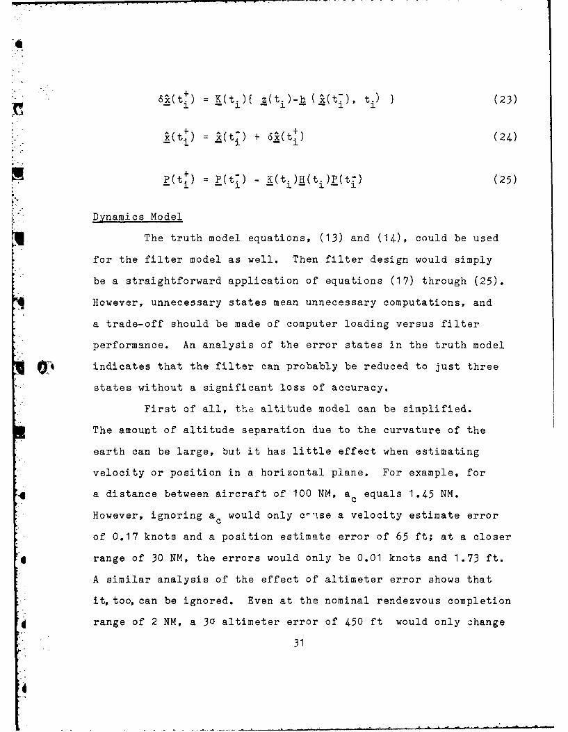
. 8x (t + ) =K(t){ Z(ti)-.h (xt , i (23)

"_(tt) = _(t) + 6_ (t+ ) (24)

P(t.) (t) - K(t.)H(ti)P(t7 ) (25)

Dynamics Model

The truth model equations, (13) and (14), could be used

for the filter model as well. Then filter design would simply

be a straightforward application of equations (17) through (25).

However, unnecessary states mean unnecessary computations, and

a trade-off should be made of computer loading versus filter

performance. An analysis of the error states in the truth model

0 indicates that the filter can probably be reduced to just three

states without a significant loss of accuracy.

First of all, the altitude model can be simplified.

The amount of altitude separation due to the curvature of the

earth can be large, but it has little effect when estimating

velocity or position in a horizontal plane. For example, for

a distance between aircraft of 100 NM, ac equals 1.45 NM.

However, ignoring ac would only c"use a velocity estimate error

of 0.17 knots and a position estimate error of 65 ft; at a closer

4 range of 30 NM, the errors would only be 0.01 knots and 1.73 ft.

A similar analysis of the effect of altimeter error shows that

it, too, can be ignored. Even at the nominal rendezvous completion

range of 2 NM, a 30 altimeter error of 450 ft would only ohange

31

4'

the horizontal position estimate by 45 ft. So, only the planned

altitude separation term, a0 , is retained in the filter model.

The filter model was further simplified by dropping the

measurement noise components from the state vector. The correlated

component, n, with a la value of 0.016 NM, is small compared to

the bias, b, which has a la value of 0.1 NM. Also, its short

correlation time makes it appear to the filter as a discrete,

uncorrelated noise. For example, with a sampling time interval

of 10 seconds, the covariance of 2 consecutive samples of n is

only 1.59 x 10-5 NM 2 . It would seem advantageous to be able to

estimate the bias. This was attempted; but as will be discussed

further in Section VI, simulations indicated that b is relatively

unobservable. When it is retained as part of the state vector,

its variance decreases very little and no noticeable improvement

in filter performance is attained. Therefore, in the final filter

design, no attempt is made to estimate explicitly b or n.

In the truth model, the along-track states are modelled

by

(t) =-vR cos 6+ vwx + Vxc + vxf(t) (8)4

But it would be difficult for an estimator to differentiate

between the random constant v xc and the slowly varying vxf. One

technique is to replace a bias plus long correlation time error

with a random walk model (Ref 13: 2-3). vxc + vxf is therefore

replaced by a single state, vxe, which is modelled by

'xe (t) = Wx(t)

32

I

where wx is a continuous white noise.

Finally, the cross-track model is simplified. The truth

model equation is

y(t) = vy c + w y(t) (7)

However, the magnitude of the random constant vyc is so small

that no attempt is made to estimate it explicitly. Instead, it

is dropped from the filter state vector and the strength of the

white noise is increased.

V What is left is a simple, three state dynamics equation

which only models the dominant states:

= 0 0 [ + 0 (-vRcos +Vwx) +

L _ 1L 0 J L L 0

= F x + B u+

0 0

1 0 Fwx

[ 1i 1w (26)

G w

These states are also the only input data required by the controller.

4 In the reduced order filter model, there is no exact way

of setting the noise strengths. Experimentation, or tuning, will

determine which values are chosen. Some reasoning can be used,

4 though, to arrive at initial trial values for Q.

33

When replacing one model with another simpler one, itwould seem appropriate for the outputs of both models to be

changing value in some similar manner. For an exponentially

correlated component replaced by a random walk, an empirically

found, useful technique is to set02

q a=

T

where G2 is the correlated process variance and T is the correla-

tion time (Ref 13: 2-3). This method was used to find an

appropriate strength for w02vxfa 1.69 x 10-8 NM2 /sec 3

Tf

A similar insight was used to set q . The one sigma

cross-track position error was said earlier to be 0.55t a NM where

ta is the time in hours since alignment. The net cross-track

error at rendezvous, then, has a variance of

a2 (t)= (0.55ta)2 + (0.55tR)2= 0.3025(tT 2 + tR 2)y aT ~ (5taR) 2 = a

where t and t are the airborne times of the tanker and

6 receiver at rendezvous. By taking the derivative of 02 (t) withy

respect to time, it is found that the variance at rendezvous is

changing at the rate of 0.605 (taT + taR) NM /hr. Because the

* variance of the random walk filter model is qy (t-t ), a

value of qy also equal to 0.605 (taT + taR) would result in a

filter model changing variance at about the same rate.

34

I

j-~

6

For a relatively long, combined airborne time at rendezvous of

15 hours, qy 2.52 x 10 3 NM2 /sec.

Measurement Model

For the tree state filter model, Eq(14) simplifies to

dT(ti) = I{x(t i ) - xT(ti)}2 + {y(ti)-YT(ti)} 2 + a 02 +v(t i ) (27)

z(ti) h(x(ti), ti ) +v(ti )

Since this is a simplification of the truth model, a

suitable variance for the white noise, v, will also have to be

found through trial and error. Primarily, v is replacing b + n,

so a reasonable first guess is to set

R G2 +G2b n

For the variances of b and n used in the truth model, the initial

filter value of R is calculated to be 0.101 NM2

Initialization

The tanker starts the filter initialization process by

estimating vR v wx, and vwy - the receiver's true airspeed and

the components of wind affecting its ground velocity. These

would be calculated from the planned indicated airspeed for the

receiver; INS computed ground speed, track, and heading; and

CADC measured altitude and air temperature. The receiver's

drift is then estimated from Eq(2). Or, if the receiver has

readouts of any of those values onboard, they can be relayed

35

over the radio and inserted manually into the computer. The

best guess of the receiver's x velocity, then, is -vRCos 6+ vwx;

and estimated deviation from this value, v (0), is zero.

v The tanker then calculates and attempts to fly the correct

offset. If no radar aiding is used, 9(0) = 0. If an estimate

of the lateral distance between the two aircraft, A , is made0

with the help of radar or other means, then it is manually

inserted and y(O) = YT(0)+ Yoe

The initial covariance matrix values are also tuned for

best performance. Since P is symmetric, only upper triangular

elements are calculated. The initial variance for y can be

taken directly from the truth model: P3 3 (0) = G2 Also,yo

because vxe Vxc + Vxf, it would make sense to choose P22(0) =

0y 2 + a2 The tanker would initially have very little infor-vxc vxf"

mation about the correlation of x,y, and vxc, so P1 2 (0) and P23(0)

are set to zero.

The only initial conditions not yet specified are

xc(0), P1 1 (0), and P 1 3 (0). A TACAN measurement at t=O can be

used to approximate those values. Approximate mean and covariance

0relations are derived using a Taylor series expansion about

y(0) and the initial TACAN measurement.

The actual distance, d, is related to x, y, and a by

d = j(X-xT)2 + (y-yT)2 + a2

The effects of altitude deviations from a are ignored, as

discussed earlier, and the equation above is rearranged to form

36

4!

a function Ax(d,Ay):Ax(d,Ay) = Id2 - Ay 2 - a2 (28)

0

where Ax = x-xT and Ay = Y-YT" Now Eq(27) is expanded to first

order about Axo = Ax(dT,A ) where dT is the TACAN measured

distance, and A^ =

Ax(dAy) = Ax0 + 3Ax (ddT) + DAx (Ay-AA)3d DAy

d = dT d = dT

Ay = AA AY = AA (29)

d-dT is the TACAN error, de; and Ay - Y =y

which is the cross-track error ye The derivatives are evaluated

and Eq(29) reduces to

_ A^

Ax(dAy) = Ax0 + dT de Y e (30)

Ax0 Axo

Now x(0), PII(O), and P13(O) can be approximated to first

order by taking the appropriate expected values and making use

of Eq(30). Remember that dT and Ax are not random, and thatT 0

de and ye are assumed to be zero mean and independent.

x = XT + Ax

xT+Axo + d T d- A Ye

Ax Ax0 0

37

.X

. xT+Ax + dT E {de}- A E {ye

Ax Ax0 0

(O) = XT(0)+ Axo(0) (31)

P 1 i(0):

x-c = (xT+Ax) - (xT+A )

= Ax - AXc

= (Ax + dT d - AS Ye ) - (X-xT)

Ax Ax o00

=dT d - A Ye

Ax Ax0 0

2P = E{ (x-Ac)

= dT 2 E{d2} -2 dTA A E {deY

Ax 2 Ax 20 0

+ AX2 E{ye a

Ax 2

0

2

P1 1(o)= 1 {d2(o)(02 + 2 ) + AS(O)a 2yo (32)Ax2 (0) T b ny

0

P 13(0):

I P 1 3 = E{(x-) (y-g)}

dT e^

:E{(A de Ax e e

38

dT- E {d ye EYe2

Ax ° Ax o

0 0

, P , , ( ) = " A ' ( 0 ) oG 2P1 3 (y) (33)

Ax (0)

Propagation

Given the simplified filter dynamics model of Eq (26),

the state transition matrix is

(iti 1 (ti- ti ) 0""i p , i -1 ( 3 4 )

1 0 1 j0 0

For a sample time of At. = t -ti , the filter propaga-1 1 1-1

tion equations, (19) and (20), can be written as follows:

1 At 0

A(t-= 0 1 + (t + )- 1 0 1ii-

0 0 I0

t. i ti ) o wxG 1 dT

which reduces to

2(t) v (t +)i xe -i

: i- (35)

39

I

And, 1 a. 0- .1 0 0

P(t-) = 1 0 P(t+ _) At 1 1

-0 0 1 0 0 1-

1 qx 0 T i 0 1 d0

LO 0 0 q 0 0 1

- hti - ii

Since P is symmetric, only the upper triangular elements need to

be calculated. The matrix equation above reduces to the

following relations:P* = Pu + 2 P12Ati + P22 At' +-q At (36a)

P12- = P12 + Pz2Ati + q At? (36b)

P22 = P22 + qxAt.i (36c)'"P 13 - = P1 3 + P2 3 At. (36d)

P 13 P2 3 (36e)

P 3 3 = P 3 3 + qy Ati (36f)

where the P terms on the right are the upper triangular elements

of P(t+ ), and the P terms are elements of P(ti-I

Update

From the filter measurement model, Eq(27),

h(x(ti)} [ { [x(ti) xT(ti)] 2 + [y(ti) . YT(ti)] 2

+ ao

: IAX(ti)2 + Ay(ti)2 + a 2 (37)

40

-4

Then, from Eq(26),H3 h {x(ti)}

H(ti) = - ,t,,

[ Ac(ti) 0 Ay(ti) (38)

df(ti) df(ti) )

where df is the filter computed distance

dfti =]A(t2 + AA(t )2 +

The state and covariance updates are now just a straight-

forward application of equations (21) through (25). The result-

ing update relations are listed in the next section.

Sometimes when measurements are nonlinear, filter perfor-

mance can be improved by adding a bias correction term to the

predicted measurement value, h(_c) (Ref 12: 225). For a single

measurement, the appropriate bias correction is given by

3 2 -

The correction term for this problem is then found to be

1 AX 2 1 AY

b = {(-- - )Pl 1 + (- - - ) P 3 3} (39)df df3 df d f

Now the predicted measurement value for forming the residual in

Eq(22) is

i i z(t i) h( (ti) + b c(t i )

,41

In effect, z was just estimated by expanding h(x)to second order

and taking the expected value. Eq(22) now becomes

!6c (tt)= K(ti ) {z(t i ) - ti)} (40)

Estimation Algorithm

The entire estimation algorithm is now summarized.

Anytime prior to rendezvous, CP coordinates, rendezvous true

course, receiver indicated airspeed, and a° are loaded into

tanker's navigation computer. At each measurement time, INS

computed tanker position is transformed to the coordinate system

illustrated in Figure 2 on page 10.

At start of rendezvous:

1. INS and CADC data are used to compute vR V, v and

6 =sin[ Vwy j-i vR

2. u = -vR cos vR .x

3. Tanker computes and attempts to establish correct offset.

Initialization:

1. If an estimate of the receiver's actual offset can be

obtained from radar or other means, AA(O) is inserted

manually. If no update is made, A (O) equals desired offset.

2. The filter is started with an initial TACAN measurement,

dT(O).

3. x and P are initialized as follows. The time argument for

42

I

all variables is t=O.

Ax^ = dT2 _A2 - a 2T y 0

AAX = xT +AX

A

V = 0xe

= YT +A

Pu1 = 21 [d (2b2 + n 2)+ AA 2 Cyo2]

P1 A c2 T fl G2 y j

P12 = 0

P2 2 = vxc 2 + cvxf 2

P 13 = yoA ^

P 2 3 0

P33 Cy 2yo

Propagation:

xc and P are propagated from sample time ti_ to t. with the

following equations. Minus superscripts indicate t- values,1" the variables on the right side of the equations are t. values.1-i

At = t. - t.1 2 .- i

Sx +( + u)At.(xe1

A A

xe xe

y

4~2A

P11 = P11 + 2PI 2Ati + P22 Atf q At 3

At. t2

PIz = P12 + P2aAti + qxtI

P22 = P 2 2 + q xAti

P13 = P1 3 + P23At.

P23 = P 2 3

P3 3 = P 3 3 + qy Ati

* .Update:

At each sample time, a TACAN measurement dT is used to update

x and P. The following relations are derived from equations

(21) through (25) with a bias correction term added. and P

elements on the right side of the equations are ti values.

Ax = x- XT

Ay = Y"- YT

df A + 2 + a 2

H1 = MC/df

H 2 = 0

H3 = AA/df

A = H12p1 I + 2HIH 3P1 3 + H 3

2P 3 3+ R

PH1 = HIP 11 + H3PI 3

PH2 = HjPI 2 + H3 P2 3

PH 3 = HjP 1 3 + H 3P 3 3

K1 = PHi/A

44 43

K2 = PH2/A

K3 = PH3/Ab c {(1/d - A 2/df )P11 + (1/d f- A/df3 )P33}

A• i d f + b cI= f c

r = dT zA+x = + Kjr

A + A +KarSxe xe

A+

y y ~+K 3 r

P+t = P1 1 -KiPHi

P 12 = Pia-KIPH 2: p2+

P 2 2 P2'-K 2PH 2

P13 = P13-KIPH3I P2+

P2 3 = P2 3-K 2PH 3+

P 3 3 = P 3 3-K 3PH 3

This algorithm is used to continually propagate and

update the receiver's state estimate for as long as needed by

the controller.

Ad

"4 Ji44

a: ,

i

V Control

Algorithms were developed to calculate the correct offset

distance, the appropriate time for the tanker to start its turn,

hand bank angle commands during the turn. For this initial

feasibility study, the control laws are based on a deterministic

dynamics model with the current receiver state estimate as input.

Tanker Dynamics

Eq(1) is appropriate for deriving the kinematic relations

foz the tanker as it was for the receiver:

v = Xa/w + v w

where v is velocity relative to the ground, va/w is the velocity

of the aircraft with respect to the air mass, and v is the-W

velocity of the wind. The tanker's heading-, W, is measured

counter - clockwise from the positive x axis as shown back in

Figure 2. Then for a tanker true airspeed of vT, the components

of Va/w are

va/wx = vTcos T

Va/wy m vT sin4

The components of the tanker's velocity in the pseudo ground

fixed frame of the INS are therefore

6 vTx = vTcoOS + vwTx (41)

7Ty = vTsinT + vwTy (42)where vwTx and vwTy are the components of wind at the tanker's

current position.45

-4

A simplified free body diagram of a KC-135 in a left turn,

with positive left bank angle $, is shown in Figure 3. L is lift,

m the tanker's mass, and g the acceleration due to gravity. In

a level turn, the vertical component of lift balances the weight,

mg, so

L cos - mg = 0 (43)

in a turn, the tanker has a centripetal acceleration, T vT,

which is caused by the horizontal component of lift. The resulting

equation of motion is

L sin T= m'vT (44)

Equations (43) and (44) are now combined to form a relation for ':

g tan)

vT

Some simplifications were employed in developing this

model, but these equations represent the principle dynamic effects

throughout the turn. The air mass and INS coordinate frame are

assumed to be non-accelerating, which they virtually are when

compared to the accelerations of a turning aircraft. Also, the

velocity vector is assumed to be along the tanker's longitudinal

body axis. For a KC-135 at cruise airspeed and shallow bank

angles, the angle of attack is small; and its effect on bank and

heading calculations is assumed to be negligible for the purposes

of this problem. As in the filter design, an implementable

control law has to be based on a model of just the dominant

effects.

46

I

Turn Point

The geometry of the tanker's turn is illustrated in

Figure 4. For a constant bank angle, constant airspeed turn, the

tanker's flight path relative to the air mass is circular with

radius of turnV T

rT T (46)

'T

The tanker wants to roll out on the refueling track with zero

lateral drift. Then, as the receiver did, it needs to apply a

drift correction; and its final heading will be

T f = 7T +

where

6 = sin- (47)

v T

From any initial heading, T' the change in the tanker's position

during the turn will equal the change in position within the air

mass plus the change due to movement of the air mass over the

ground. Then

AXT XTf XTo

= rT sin (7+6) - sinPoj + vTTVwTW

rT I-sin 6- sin T + VwTxT (48)

where xTf and xTo are the tanker final and initial x coordinates

and T is the duration time of the turn. T can be found from

T A T = 7+6-To (49)

47

L

Shorizon

mg

Figure 3. Tanker Free Body Diagram (Tail-on view)

x

iyqi0 y¢

/T• /

6 -T

Rollout os Turn Point

Figure 4. Rendezvous Turn Geometry

48

By substituting Eq(45) into Eq(46), it is found that

.. vTrT T (50)

g tan

Also, substituting Eq(45) into Eq(49) results in

A;4 v T

T = T (51)g tan

Now these relations for rT and T are used in Eq(48) to derive

V TAXT - T v (-sin 6- sin )g tanT

+ (Tr+ 6-) Vw- (52)0 x

Similarly, it can be shown that

SAYT YTf YTo

=rT [cos 6 + cos 'K] + VwTYT (53)

," VTT" {- { T (C os 6 + Cos Yo) + ( + P 0o v wT y } (54)

, g tan

Eq(54) can be used directly to determine the nominal

offset distance. For the tanker to fly towards the receiver

parallel to the refueling track, a drift correction of -6 must

be applied. The change in sign is because 6 is calculated for

the rollout heading, and the tanker is initially flying in the

opposite direction. Then Yo= -6 and the desired offset is

S T { 2 vTcos 6 + (Tr+ 26) vwTy (55)g tan

49

6

where n is the nominal bank angle.

The present procedure uses a nominal bank angle of 30

degrees. But 30 degrees is also the tanker's maximum bank angle

under normal conditions. Therefore, a shallower nominal bank

angle must be used if bank angle corrections are to be applied

during the turn. With no cross-wind, a nominal bank angle of

25 degrees requires about a 9.6 NM offset. Nominal offsets

greater than that were considered unreasonable due to airspace

restrictions imposed by air traffic control.

The tanker attempts to establish the nominal offset

distance, but the computed time to turn should be based on the

tanker's actual offset and heading - not the nominal. For

example, the tanker may actually be wider than the computed

offset and its initial heading other than -6 while it is correct-

ing to course. In that case, it should turn earlier and with

a shallower bank angle than nominal. The ability to compute

other than nominal solutions does not exist with the present

method but could be implemented with the proposed system.

To compute b r' the required bank angle to roll out along

the receiver's estimated flight track, y - YT is substituted

for AYT and Eq(54) is solved for b:

$ *r = tan c)(VT(Cos6+ Cos T0 )+(7+6- 0 ) vwTy) (56)

Given r' the time required for the turn is

Ur

50

Q1

Tr =(r+6-0v (57)

g tan(r

which is derived from Eq(51). If the tanker turns at the current

time, its x coordinate at rollout will be

- XTf = XT + Ax T

where AxT is found from Eq(52). The receiver's position at

tanker rollout is estimated by

A A A

X= x+ v Tf x x r

where

(-VRCoS6+ v) + 0e (58)

The tanker wants to roll out 2 NM in front of the receiver.

0 If it turns tooearly, its miss distance in front of the receiver,

A

X m is

m= xf -2XTf

But Xm is decreasing at the rate of the two aircraft's closing

speed, vTx-^x. The estimated time to go until the turn should

.4 be started, TTG, is then given by

TTG = m (59)A

VTx x

TTG is counted down between updates, and the tanker turns with

bank angle r when TTG <0

51

a.

The algorithm for determining the turn point is now summarized:

A. The tanker computes and attempts to establish the correct

offset for a nominal bank angle 4n:v1. 6 = sii wTv

vT

2. os = V{2vTCOS6 + (+ 26 )v wTyg tan wT

B. The required bank angle and time to go until turn are

updated based on actual tanker position and heading:

1. AT = 7+6-Y o (60a)

1 v T

2. = tanT (VT(COS5+COS To )+ AyvTylJ (60b),:" g(^_yT)

3. T T (60c)g tan

_VT

4 .AxT ={VT(-sin6-sinTO) +ATVwT x } (60d)g tan ¢r

5 .XTf x + Ax (60e)

Tf = T AT

6. vx = (-VRCoS6+ Vw) + xe (6Of)

7. xf = x + 'xTr (6 0g)

8. A. = Xf" 2- XTf (60h)

A

9.TTG = m (60i)A. VTx x

52

Closed Loop Control

As was stated previously, one of the primary potential

benefits of the proposed system is that it would enable the

tanker to use closed loop control during the final turn to

rendezvous.

The present procedure is entirely open loop: the tanker

maintains a constant 30 degrees of bank until reaching the

1refueling heading. A simple improvement would be to apply

cross-track control only. At each update time, the tanker would

compute the required bank angle to roll out in front of the

receiver using Eq(56). The result should be decreased cross-

track error at rollout, which would mean less lateral maneuvering

would be required of the receiver to complete the join-up.

V arUsing bank angle control to minimize the along-track

error also, is more complicated. That is because, in general,

the tanker cannot get from its present position and heading to

a zero error rollout condition with a constant bank angle. A

method of solving the problem which was used in the simulations,

is based on the following basic algorithm:

1. Compute r to roll out on the receiver's estimated track.

2. Determine the x miss distance if r is used.

3. Adjust 4r based on x miss. If the tanker would roll out

in front of the receiver, decrease the bank angle and vice-

versa.

The basic idea, the4 is to see if an exact solution exists from

4 the present position and heading. If one does not, adjust the

53

bank angle to fly towards one.

The first two steps of this algorithm are solved by

equations (60a) through (60h). The remaining question is then

how much to correct An ad hoc method was used based on the

following insights. If the tanker would roll out in front of

the receiver, it needs to fly a longer path to the rendezvous.

Similarly, if it would roll out behind the receiver, more cuttoff

and a more direct route should be flown. A measure of the effect

of a bank angle change at the present position, is the change

in arc length it would cause if held until rollout. The control

law was then based on the following equation:

rTcAY - rTrAY = k m (61)

where rTr is the radius of turn for 4 r' Xm is the projected miss

distance using 4r' rTc is corrected radius of turn, and k is a

proportionality constant which will be tuned for best performance.

In other words, the arc length is increased by an amount propor-

tional to the miss distance. When Eq(61) is rearranged, the

equation for rT is

k Ax mr = + rTr (62)AT

This law exhibits the following desirable characteristics.

If Xm is zero, then 4r is an exact solution and rTc equals rTr.

The change in turn radius is proportional to ^xm, and inversely

proportional to AY - the further away the tanker is from roll-

out, the less correction needed.

54

Eq(61) also gives some insight into setting k. A value

of k=1 would increase the arc length by the amount of x m Since

both aircraft are flying at about the same speed, if the tanker

would maintain rTc until rollout, it would roll out at about

the same time that the receiver would reach the rollout point

based on $ . A good initial trial value for k would then be 1.r

The ad hoc control algorithm is then:

1. - 7. Same as equations (60a) through (60h).

2Ii VT;" 8 . rTr . . .g tan

r

9. rc =rTr +

2

10. c = ta: T

grTc

At this point, the 30 degree maximum bank angle restriction

should be recalled. For both the turn point and the closed loop

bank angle control algorithms, the following conditional state-

ment was added after step 2. (Eq(60b)):

2a. If $r < 30 degrees, then set 4'r=30 degrees.For the closed loop control algorithm, if 'r is greater

hr

than 30 degrees, ac should also be set to 30 degrees and the

algorithm stopped at that point. In that case, the tanker is

headed for an overshoot of the desired rollout track: it cannot

turn any tighter, and a shallower bank angle will only make the4

overshoot worse. Also, if YT is greater than , the tanker has

55

4

*already overshot the receiver's estimated cross-track position,

and the full 30 degrees of bank should be used.

So far, a mathematical model of an air refueling

rendezvous has been created, and estimation and control algorithms

have been developed. The last major task of this study is to

do an initial evaluation of the filter and controller designs.

56

tI

VI Simulation Results

Computer simulations of a typical rendezvous were used

for an initial analysis of the estimator and controller designs.

Simulation

The filter and controller were evaluated using Monte

Carlo simulations. The statistics for each Monte Carlo run

were calculated from the results of 30 separate, simulated

rendezvous. In each rendezvous, a different set of random

variable realizations was simulated.

The receiver's dynamics and the TACAN measurements were

modelled exactly as described in the summary of Section III.

The tanker's dynamics were modelled by Eqs(41), (42), and (45).

In each case, the tanker started from a position along the minus

0y axis with an initial flight path direction parallel to the

refueling track. vR and vT were both set to 396 knots, which

would be typical for a refueling altitude of 25000 ft and

standard day conditions.

SOFE (Ref 14) and SOFEPL (Ref 15), two computer programs

developed for Monte Carlo simulations of Kalman filter design

problems, were used to accomplish the runs and generate the

appropriate outputs. The extended Kalman filter equations

discussed in Section III are automatically implemented in SOFE

with one exception. Rather than the standard update equations

given by equations (21) through (25), a Carlson update (Ref 14:

28-29) is used. This type of update is algebraically equivalent

to the standard form, but it has numerical stability and accuracy

57

advantages when used on a finite wordlength computer. Whether

those advantages outweigh the inherent, increased computational

requirements for this problem, would be an area for future study.

- To ensure a standard means of comparison, the same

control algorithms were used for all filter evaluations. The

turn point algorithm given by Eqs(60a) through (60i), and the

cross-track controller, which only uses Eq(56) at each update

time, were used. Also, the control algorithms used the true

state values rather than the estimated states as input. For the

same reason, each controller was evaluated using the same filter

algorithm to provide the estimated state inputs.

Filter

The big unanswered question about the proposed system

is how much information can be gained from TACAN, distance-only

measurements. Ideally, the filter would be so accurate that

radar would not be needed. Then, accurate rendezvous could be

conducted even if radar contact is lost or never achieved. The

filter would be started as soon as the receiver passes the initial

point. An accurate estimate of the receiver's cross-track position

would then be used by the tanker to establish its initial offset.

Unfortunately, though, the initial simulations indicated that

attaining such a degree of accuracy may not be feasible.

4 A 7 state filter which modelled all of the states except

the short correlation time component of TACAN error was initial-

ized at simulated 100 NM ranges. The results indicated that,

as suspected, some of the states were relatively unobservable.

58

V The filter predicted error standard deviations, as measured by

the square roots of the diagonal elements of P, decreased very

little for the TACAN bias, altimeter error, and constant vKyc

states. Between the start and finish of the rendezvous, the

predicted standard deviations only decreased about 10% for b,

1% for v y, and virtually not at all for a e . Also, those slight

improvements for b and v yc did not occur until about the last

60 seconds of the rendezvous.

For an initial 100 NM range and a value of 6.15 NM,yo

both the 7 state filter and the 3 state filter described in

Section IV were very difficult to tune. The filters produced

biased estimates; and they greatly overestimated their own

accuracy: the diagonal elements of P quickly converged to values

much less than the true error variances. An accurate cross-

track estimate never could be achieved until the range decreased

considerably. In Figure 5, the standard deviation of the filter's

actual cross-track estimate error, computed for each sample time

of a typical Monte Carlo run, is plotted. Notice that at t=310

seconds, which corresponds to about a 30 NM range, the actual

filter error had a standard deviation of around 4 NM. The tanker

would be better off using radar, with its assumed la error of 1

NM at that range.

When it appeared that no progress was being made in

designing an adequate estimator for that "worst case" situation,

attention was shifted to a more restricted problem. It was

assumed that the tanker would use radar to establish its offset

59

to

CD0

F-d

CE3

U-) 0

f !D 0

Li W 0

9

CD D0 L

Li 0

oh

600

QI

and to obtain a relatively short range initial estimate of the

receiver's position. The filter would then take over and pro-

pagate and update the state estimate through the rest of the

rendezvous. The advantage of even this restricted case is that

it would provide a state estimate for turn point calculations

and bank angle control during the turn. The radar is good for

initial estimates and positioning, but the one onboard the KC-135

cannot lock on a target. Therefore, it could not easily be used

for periodic updating during the turn since all radar updates

must be entered manually.

The filtering was initiated at a simulated range of 30

NM, giving about a 50 second period before reaching the turn point.

This shorter range also makes the velocity assumptions about

0 i the receiver more valid. By 30 NM, the receiver should have

completed any initial maneuvering or altitude changes that may

have been necessary, and its flight path should be fairly stable.

The results of the 3 state filter simulations are plotted

in Figures 6, 7, and 8. All of the filter parameters were tuned

to the values discussed in Section IV. In each figure, the

statistics of the actual filter error, computed from the time

histories of 30 simulated rendezvous, are depicted. The actual

filter error is defined as the difference between the appropriate

* truth state value and the filter estimated state value. The

center, solid line represents the average error; the two broken

lines are the mean error plus and minus the standard deviations;

and the two dashed lines are the filter predicted standard

61

deviations, calculated as the average square root value of the

*i appropriate diagonal element of P.

Each of the plots demonstrate some desirable filter

characteristics. The mean error stays near zero. Also, the

filter predicted standard deviations fairly closely bracket the

actual mean plus standard deviation plots. In other words, the

filter performs its updates based on an internal model which

closely approximates its actual performance.

The plots also indicate, however, that the accuracy

does not improve significantly from the initial uncertainties.

For the x position and velocity components, no noticeable

improvement is made until about t=120 sec, which is when the

tanker is approximately halfway through the turn. Meanwhile,

the y estimate just exhibits a modest, steady improvement.

Some of the filter parameters were varied, but no

noticeable improvement was achieved. For example, shorter sample

periods were used. The results of Figures 6 to 8 were based on

a simulated time between measurements of 10 sec. For Figures

9, 10, and 11, a shorter period of 2 sec was used. The actual

error statistics stayed about the same.

Another interesting result was found when experimenting

with the simulated TACAN errors. The TACAN bias error standard

deviation of 0.1 is large compared to the short correlation

time component's constant variance of 0.016 NM. However, if the

bias error is removed entirely from both the truth and filter

1462

I

00L.) $0

I; 4_ I!

CLL

C-)O

CE2 E

I

Z / or%3(Wf) ~zlS~-

630

CD H

LCc

LiL

C-)

coic

z a 01 0a 0 t-:C ..) 1 4.)J/N80.133W IS3A'103 -

toCE4

4 64

!i 4-3I

a: oLO0

LJ1

- 4r.

r*r

r 4-)

S* *-so 0

(W JOJJ 3lWII NW.I0 1aLb

651

1-

K -3

Li-

U-)~

4P 4J oo 0

QWN III 3641.3NOIS -

66I

LL (

cr:

- 0-

CD ,

U) 4)

C- a:o(-- 0l

4 67

.

44

CDC

czD

Loo

L.I.CT) I I U

CD U

CT)d

C.D

I ri

010S- 1. 1

68

.. ....

models, the filter performance is still about the same. The

cross-track error statistics for this case are plotted in Figure

12. The plots are almost identical to those in Figure 8. This

result indicates that not much would be gained by being able to

estimate b or calibrate it out of the TACAN.

All of the simulations seemed to indicate that the results

plotted in Figures 6 to 8 represent a practical limit for the

extended Kalman filter. The driving constraint on filter

performance does not seem to be the number of filter states, the

sample period, or the magnitude of the TACAN bias error. The

rendezvous geometry itself, would intuitively seem to be the

primary constraint. Because the aircraft are approaching each

other nearly head-on, not much cross-track information is avail-

able until late in the rendezvous. Investigation of different

rendezvous geometries might be a suitable area for future study.

The improvement in estimation accuracy over the initial

uncertainties is not significant. But the extended Kalman filter

does seem to be a relatively simple, stable method of generating

a receiver state estimate up through completion of the rendezvous.

With the present method, the tanker has no useful means of estima-

ting the receiver's state once the turn is started.

Controller

The most important question of this study still remains

to be answered: what improvement in rendezvous accuracy might

be achieved with the proposed method? To answer that question, the

69

LiiiA i

Li 9 E--

L

LO

C:)

C4-)

CD

C-, 1

C22

700

control algorithms of Section V were incorporated into the

Monte Carlo simulations. For each case studied, the 3 state

filter with 10 second updates provided the inputs to the controller.

Each rendezvous was initialized at a 30 NM range and was terminated

when the tanker had turned to the refueling heading. The rollout

errors were then calculated as

xm = x(tf) - 2 NM - xT(tf)

! Ym y(tf) - YT(tf)

where x and ym are the rollout miss distances, x and y are the

true receiver position coordinates, and tf is the final, or

rendezvous completion, time. For each Monte Carlo run, 30

simulated rendezvous were used to compute the means, standard

deviations, and root mean square statistics for xm and y

To form a basis for comparison, the present rendezvous

method was also simulated. For-the airspeeds and zero wind

conditions used in the simulations, the turn range chart (Ref 16:

3-5) gives a nominal offset of 7 NM and a turn range of 17 NM.

In the first case studied, it was assumed that the tanker

had maneuvered to the computed offset distance, based on ^, prior

to the turn. The only actual offset errors were then due to the

A estimate errors. For the present, open loop method simulations,

this meant that the tanker had established an estimated 7 NM

offset, but the actual offset had a standard deviation of 1 NM

due to radar estimate errors. For the controlled rendezvous,

the tanker started from an estimated offset of 9.6 NM - the

71

nominal offset for a 25 degree bank turn. Again, the actual

offset varied from this mean value with a la error of 1 NM.

The results are listed in Table 1. Since the present

method has no means of improving its estimate of the receiver's

y position, its la value for Ym is about equal to the initial

radar estimate error. Also notice the large bias errors at

rollout. These would primarilly be due to using the whole mile

range values from the turn chart, though some of that error can

be reduced by interpolating values from the chart.

The cross-track controller only used Eq(56) at each update

time to compute a bank angle which would roll the tanker out on

course. The l ym value decreased by a factor of 4. However,

there is a slight increase in the error statistics for xm . That

is because when the turn is started, the filter still has about

a .4 NM error standard deviation. As a better estimate

becomes available during the turn, r changes and so, therefore,

Table 1. Rollout Error Statistics

Xm (NM) Ym (NM)

Controller m a RMS m a RMS

Open Loop .83 .71 1.09 .35 1.11 1.16

Cross-Track .89 1.06 1.38 .14 .23 .27

*4 Closed Loop:

k=2 .09 .84 .84 .10 .43 .44

k=3 -. 21 .54 .58 -.10 .41 .42

72

a.

does P. The change in the turn rate from that predicted at the

start of the turn, causes the rollout time and hence x to vary.

Closed loop control along both axes was simulated next.

Results for values of k equal to 2 and 3 are listed. With only

a slight increase in the standard deviation of ym, the statistics

for xm improved considerably. Most of the mean error is

eliminated. For k=3, the root mean square error is about half

of what it is for the open loop and cross-track controllers.

Since the desired values for xm and ym are zero, their RMS values,

where RMS = im2+ 2 are an appropriate, comparative measure

of controller performance.

The values for k equal to 2 and 3 were selected from the

results of a larger set of runs. In Figure 13, the RMS miss

distances are plotted for values of k between 0 and 10. The

case of k equal to zero implies cross-track control only: the

bank angle which minimized ym was computed, and no adjustments

were made to reduce xm. As k was increased above zero, the RMS

values for xm decreased, while the ym RMS values increased

slightly. However, for k equal to 9 or more, the bank angle

corrections were too great, and the controller produced increas-

ingly large rollout errors. At k equal to 12, the RMS values

for xm and ym were 9.3 and 3.0 NM respectively. The controller

* did not seem to be particularly sensitive to changes in gain

in the range of k equals 2 to 6. The x miss distances were

improved over those of the cross-track controller, and the y miss

* distances remained small.

73

0- 0

4c

000

0 02

02/ r-1CH

74-

A Monte Carlo run was also conducted in which the

controller inputs were the true states and not the filter estimates.

K. For a gain of k equal to 3, the resulting xm RMS value of 0.17 NM

and ym RMS value of 0.09 confirmed that there were no basic flaws

in the closed loop control concept itself.

One other case was simulated. A turn from other than

nominal conditions was modelled. Such an initial error might

be due to pilot error, insufficient time to correct to the

desired offset, weather avoidance, and so on. For the open loop,

cross-track, and closed loop controllers, the turn was started

from an offset 2 NM wider than nominal, and 5 seconds earlier

than it should have been.

For this case, the differences in controller performance

were more pronounced. The results are listed in Table 2. The

open loop controller had large mean errors because it never tried

to compensate for the initial deviation. The cross-track controller

reduced the ym RMS value by a factor of 10, but it did not correct

Table 2. Rollout Error Statistics - Turn Initiated FromOther Than Nominal Conditions

x m(NM) Ym(NM)

Controller m a RMS m a RMS

* Open Loop .96 .70 1.19 -1.22 1.07 1.62

Cross-Track .93 1.02 1.38 .04 .13 .14

Closed Loop (k=3) -.15 .74 .75 -.09 .39 .40

75

-°

for along-track errors. Finally, the closed loop controller had

significantly lower RMS values than the present method for both

xm and y m That was because the closed loop corrections reduced

the mean rollout errors to near zero.

Even though the filter does not supply a particularly

accurate estimate of the receiver's state, the closed loop

controller and, to a lesser extent, the cross-track controller,

exhibit some advantages over the present open loop method.

The cross-track RMS errors are reduced considerably. The closed

loop controller also moderately reduces the RMS along-track

error. Additionally, these control algorithms compute rendezvous

solutions for other than nominal offsets and headings, and can

correct for deviations during the turn.

74

r 76

4° .

-

VII Conclusions

The purposes of this research were to develop a digital

estimation and control method for conducting air refueling

rendezvous, and to evaluate its feasibility and possible benefits.

For this study, the design was constrained by present, onboard

KC-135 navigation equipment, and the basic geometry of the

current method.

A 3 state extended Kalman filter, which only incorporates

air-to-air TACAN distance measurements, is not a very accurate

estimator, and it appears that a radar estimate would be needed

to initialize the filter. However, it does appear to be a simple,

stable method of generating a receiver state estimate throughout

the final portion of the rendezvous.

Using the filter generated estimate, a single equation

control law can significantly reduce cross-track error at

rendezvous completion. A control law can also be implemented

which decreases the along-track error as well. Using the closed

loop control algorithm, the root mean square, cross-track error

at rollout was reduced by up to 75% over the present method;

and the along-track error was reduced &3 much as 47%.

The proposed method has two main advantages over the

present method. It can compute rendezvous solutions from other

than nominal cinditions; and it generates a receiver state

estimate which enables the tanker to use closed loop control

throughout the rendezvous.

77

The proposed system is entirely compatible with present

rendezvous procedures and onboard KC-135 navigation equipment.

Incorporating such algorithms in an INS "rendezvous mode" could

be a valuable aid for conducting air refueling rendezvous.

78

VIII Recommendations

The computer simulation results do indicate that the

proposed system has some potential advantages over the present

method. The next step should be a more complete analysis of the

models and designs developed here. Several areas for further

study immediately come to mind.

The truth model could be improved with a stochastic

'I model for the tanker's dynamics as well as the receiver's.

Such a model would be better for evaluating different controller

designs because the effect of deviations during the turn could

'be evaluated. In this study, only initial deviations were

simulated. Such a model could also provide a basis for a

stochastic control design analysis.

There are several estimation issues yet to be considered.

A sensitivity analysis of the filter to modelling errors should

be done, and different aircraft types and airspeeds should be

simulated. The effect of the rendezvous geometry on observability

could also be investigated.

A present hardware constraint was imposed for this study.

However, given the limited filter accuracy achieved, the potential

advantages of incorporating other equipment might be considered.

For example, the AN/ARN 139 (V) TACAN system which provides

air-to-air bearing as well as distance information could be

considered (Ref 17).

7• ' 79

°a

S." The potential advantages of closed loop control were

investigated, but only one algorithm was developed. Other ad

hoc methods could be investigated as well as stochastic control

methods.

A vital area which was barely considered in this study

is the onboard computer. The estimation and control algorithms

need to be evaluated partly on the basis of computation time,

memory requirements, and so on. Also, the algorithms developed

here might be simplified further.

Very little work has been done in the past on the air

refueling rendezvous problem. Therefore, research in just

about any area of the problem might result in significant

improvements.

48

-I

.

References

1. Delco Electronics Division. Technical Description, CarouselIV-E Inertial Navigation System. S77-53. General MotorsCorporation, Santa Barbara, California, June 1977.

2. Widnall, William S. and Grundy, Peter A. Inertial NavigationSystem Error Models. Intermetrics Incorporated, Cambridge,Massachusetts, May 1973. (AD 912 489L).

3. 443d Technical Training Squadron. Academic Student Guide,C-141 Pilot Air Refueling Qualification Course. Documentno. 4P7-2. Altus Air Force Base, Oklahoma, August 1980.

4. Bobick, J.C. and Bryson, A.E.,Jr. "Improved Navigation byCombining VOR/DME Information and Air Data," AIAA Paper

.. 'No. 71-928, AIAA Guidance, Control, and Flight MechanicsConference, Hempstead, New York, August 1971.

5. Maybeck, Peter S. Stochastic Models, Estimation, and Control,Volume 1. Academic Press, New York, 1979.

6. Winter, H. "Experiences in Flight Testing Hybrid NavigationSystems," AGARD Lectures Serie No. 82, Practical Aspectsof Kalman Filtering Implementation, May 1976. (AD-A024 377).

007 7. AFM 51-37. Instrument Flying. Department of the Air Force,Washington, D.C., December 1976.

8. Maybeck, Peter S. Filter Design for a TACAN-Aided Baro-Inertial System with ILS Smoothing Capability. AFFDL-TM-74-52,Air Force Flight Dynamics Laboratory, Wright-Patterson AirForce Base, Ohio.

9. Sherard,G.W. "Range Noise Analysis of the ARN-118 TACAN,"Internal letter, Rockwell International, Collins Groups,Cedar Rapids. Iowa, 11 March 1981.

10. Collins Government Avionics Division. Collins TCN-118(AN/ARN-118(V)) Airborne TACAN System. Description 523-0765893.Rockwell International, Cedar Rapids, Iowa, 1 April 1979.

11. Luciani, Vincent J. Accuracy Test of an Air-to-Air Ranaingand Bearing System. Report No. FAA-RD-77-59, June 1977.

4 TU A043392).

12. Maybeck, Peter S. Stochastic Models, Estimation, and Control,Volume 2. Academic Press, New York, 1982.

4

°8

I

13. Wauer, John C. "Practical Considerations in ImplementingKalman Filters," AGARD Lecture Series No. 82, Practical Aspectsof Kalman Filtering Implementation, May 1976. (AD-A024 377).

14. Musick, S.H. SOFE: A Generalized Digital Simulation forOptimal Filter Evaluations, User's Manual. AFWAL-TR-80-1108,Air Force Wright Aeronautical Laboratories, Wright-PattersonAir Force Base, Ohio, October 1980.

15. Musick, S.H. SOFEPL: A Plotting Postprocessor for 'SOFE',User's Manual. AFWAL-TR-80-1109, Air Force Wright

Aeronautical Laboratories, Wright-Patterson Air Force Base,Ohio, November 1981.

16. T.O. 1-1C-1-3. KC-135 Flight Crew Air Refueling Procedures.Department of the Air Force, Washington, D.C., 1 November1980.

17. Collins Government Avionics Division. Collins AN/ARN-139(V)Airborne TACAN. Technical Data Sheet. Rockwell International,Cedar Rapids, Iowa, 25 February 1981.

I 8!82

VITA

Captain James T. Rivard was born in Detroit on November

30, 1952. In 1970, he graduated from Divine. Child High School

in Dearborn, Michigan and entered the United States Air Force

Academy. There, he was awarded the degree of Bachelor of Science

in Astronautical Engineering in 1974. After pilot training at

Williams Air Force Base, Arizona, Captain Rivard was assigned

to the 30th Military Airlift Squadron, McGuire Air Force Base,

New Jersey. For five years, he flew as a C-141 pilot, aircraft

commander, and instructor pilot until he entered the Air Force

Institute of Technology in 1981.

Permanent address: 2216 Drexel

Dearborn, Michigan 48128

83

.o

7 UNCLASSIFIEDSECURITY CLASSIFICATION OF THIS PAGE (When Data Entered)

REPORT DOCUMENTATION PAGE READ INSTRUCTIONSREPORT ROPORENTATRON GE BEFORE COMPLETING FORMiREPO R 2. GOVT ACCESSION NO. 3. RECIPIENT'S CATALOG NUMBER

.i. AFIT/GA/EE/82D-I r),4. TITLE (and Subtitle) S. TYPE OF REPORT & PERIOD COVERED

DIGITAL ESTIMATION AND CONTROL FOR:.. MS ThesisK- AIR REFUELING RENDEZVOUS S. PERFORMING ORG. REPORT NUMBER

7. AUTHOR(&) a. CONTRACT OR GRANT NUMBER(s)I James T. Rivard

Capt

9. PERFORMING ORGANIZATION NAME AND ADDRESS 10. PROGRAM ELEMENT. PROJECT. TASKAREA & WORK UNIT NUMBERSAir Force Institute of Technology (AFIT-EN

Wright-Patterson AFB, Ohio 45433

I. CONTROLLING OFFICE NAME AND ADDRESS 12. REPORT DATE

December 198213. NUMBER OF PAGES

9_94Is. MONITORING AGENCY NAME & ADDRESS(If different from Controlling Office) IS. SECURITY CLASS. 'of rhi FePort)

Unclassified

1Sa. DECLASSIFICATION DOWNGRADINGSCHEDULE

16 OISTRIBUTION STATEMENT (of this Report)

Approved for public release; distribution unlimited

7. DISTRIBUTION STATEMENT (of the abstract entered In Block 20, if different from Report)

18. SUPPLEMENTARY NOTES I . . 10-17.

4-:'.r4' JAN 1 8L"" Doe O l ln low iiis'vt,, r.! revelopmeati ~A yo I ngIUtuto ol lec:inologY¥ (A191.

Wrtgt-Pett om MR On 4ti

19. KEY WORDS (Continue on reverse side if necessary nd identify by block number)Estimation Kalman FilterControl ModelAir RefuelingRendezvousTACAN

20. .ABSTRACT (Continue on reverse aide If necessary and identify by block number)Estimation and control algorithms were developed for use by a

tanker aircraft conducting an air refueling rendezvous. Astochostic model of a typical rendezvous was developed first.

- Then an extended Kalman filter which uses air-to-air TACANdistance measurements was designed. Also, algorithms werederived for computing the tanker's appropriate offset, turn point,and closed loop bank angle commands during the final turn of a

4 DD ,jAN73 1473 EDITION OF I NOV S IS OBSOLETE UNCLASSIFIEDSECURITY CLASSIFICATION OF THIS PAGE (I74en Date Enter&

TT1nT.A STPTPDSECURITY CLASSIFICATION OF THIS PAGE(Wen Data Entered)

point-parallel rendezvous.In Monte Carlo simulations, a 3 state extended Kalman filter

provided a stable, though limited, means of estimating thereceiver's position and velocity throughout the rendezvous. Also,the control algorithms exhibited two advantages over the presentrendezvous method: turn point solutions could be computed forother than nominal offsets and headings, and bank angle commandsduring the turn reduced position errors at rendezvous completion.When compared to the present method, root mean square, cross-track distance errors at rollout were reduced as much as 75%,and along-track errors were reduced up to 47%.

4

!.

UNCLASSIFIEDSECURITY CLASSIFICATION OF THIS PAGE(eWhn Date Entered)

FILM72

3=8