ad-a124 841 a modified iolmoooroy-sninov … · 4 ?arariater g~ai~ina idistribution with unknown...
TRANSCRIPT

AD-A124 841 A MODIFIED IOLMOOOROY-SNINOV ANDERSON-DARLING AND 12CRAMER-VON RISES TEST F..CU) AIR FORCE INST OF TECH
.... RIOHT-PATTERSON AFB OH SCHOOL OF ENGI. P J VIVIRNO
UNCLASSIFIED DEC 82 AFIT/GOR/R/2D-4 Fla 12/1i N

p..W
VI LIIILu
1..25 1111.4 111 6
MICROCOPY RESOLUTION TEST CHART
NATIONAL BUREAU OF STANDARDS1963-A
-- %7

V1 0
1met
AESCN-DARLINcG, AND CRAMER-VON miIss r, T FORi THE GA:MMA
DXSMIBUTION WITH UNKNOWVINLOCATVON Ai"D SCALE PAflAmETiERS
TiEzSIS
GFIT/GR/MA/ 820 -4 Philip J. VivianloAFIT/V Capt UA
This document has bee pproved -
L 4to public release and sle; itsFE 2 4 093
distributionl is unlimited.
DEPARTMENT OF THE AIR FORCE;OAIR UNIVERSIY (ATC)
AIR FORCE INSTITUTE OF TECHNOLOGY1
Wright- Patterson Air Force Base, Ohio
*too

U,2C LASS I FI ECSECURITY CLASSIFICATION OF THIS PAGE (Whotn Data EFntered*_________________
REPOT DCUMNTATON AGEREAD INSTRUCTIONSREPOT DCUMNTATON AGEBEFORE COMPLETING FORM1. REPORT NUMBER 12 OTACS1N NO. 3. RECIPIENT'S CATALOG NUMBER
AFI T/GOR/tMA/32D-4 5.GV CE9
4. TITLE (and Subtitle) 5. TYPE OF REPORT & PERIOD COVEREDA Mt:,IFIED !<OLIMiOGOROV-3-MIRNOV, ANDFERSCN,\-DARLING, AND CRAME.-VN NIISES-TEST FR U T~THE GA;IAA DISTR.ESUTI(>J 'NITi U'4t(NO'AiN 6.PEFRIGO.RPRTNMR
LOCATI ON AND SCALE PARAM ETERS7. AUTHOR(&) S. CONTRACT OR GRANT NUMBER(@a)
Philip J. Viviano, Capt., USAF
9. PERFORMING ORGANIZATION NAME AND ADDRESS 10. PROGRAM ELEMENT, PROJECT. TASKAREA & WORK UNIT NUMBERS
Air Force Institute of Technolog/AFIT-Ee.!right-Patterson AFi3, Ohio 45433
1I. CONTROLLING OFFICE NAME AND ADDRESS 12. REPORT DATE
December 198213. NUMBER OF PAGES
14. MONITORING AGENCY NAME & ADDRESS(II different from Controllfig Office) 15. SECURITY CLASS. (of this report)
UrICLASSIFIED15a. DECLASSI FICATION/ DOWNGRADING
SCHEDULE
1S. DISTRIBUTION STATEMENT (of this Report)
Approved for ?,uhlic release; d'istribution unlim~ited.
'7. DISTRIBUTION STATEMENT (of the abstract entered in Block 20, 1 .dfrent from RePort)
* 1S. SUPPLEMENTARY NOTESApi 1R 7p d Iox ibI rle. LAW APR 1907.
11 eder .yl ! Si' TRi'OLAV~f
Eircto Dean for Research and Professional DevelopmlJANi~ 1980 Forenstiutei atTchnology (AW&L
19. KEY WORDS (Continue on reverse side If necesary and identify by block number)m~oified Kolmoorov-Smnirnov 2a m. a Listribution% oditied ,%nderson-narlingj 'onte Carlo Sim~ulation11odif led Crat.er-von rises Critical Value3
* Zry-erical Distribution Function Statistics
20. ABSTRACT (Continue an reverse aide if necessary and Identify by block number)
'lie .,o1:.oorv-3mirnov, Anlerson-rarling, and Crar:'er-von ',,is--sstatistics are used to develop a ne,., test of fit for the thr-3a-
4 ?arariater g~ai~ina Idistribution with unknown location and s~calecarariaters. The ioodness-of-fit tests are valid for sa1 -zplesizes, n =5,10,.,.3C, and shapa paraoteter, K
DO I JAN72 1473 9017014orNOV 411 S OBSOLETE JCASbI~SECURITY CLASSIFICATION OF THIS PAGE (RNien Date Entered)

ULNCLASSI FI L"JSECURITY CLASSIFICATION OF THIS PAGE(Whmu Dora Entered)
A power investigjation of the tests is partormed against tenalternative distributions. The m~ost powerful test againstthe alternative distributions is the Cram~er-von .Iises, fol-lowed closely by the Anderson-Darling; the Xol,.ogorov-Sriirnov is~ the least pow,:rftu1.
A functional relationshi.? between the critical values andshape paraicieter is investigated for each test. The criticalvalues can be expressed as a function of t-,e inverse of thesquare of the shape parameter.
SECUPITv C1. 4SSI~ V, A -1

p--
W A .'.OD1F l D KOL>'!OGOflOV-S ,' IRNOV,
ANDERSON-DARLIN G, AND CRAMER-VOz MI;ES ''ST FOR THE GA,.MA
DISTRIBUTION WITH UNKNOWNLOCATION AND SCALE PARAMETERS
T*iEgSIS
AFIT/GOR/YIA/82D-4 Philip J. Viviano
Capt USAF
L
,.L,
,. .. ..-... ,*--

-. ~~~~~ ~~ ..w-.--~-- . .. .- .. .. .- . ..
AFIT/GOR/MA/8 2D-4
A MODIFIED KOLMOGOROV-SMIRINOV,
ANDERSOM-DARLING, ANO CRAMER-
VON ,,IISES TEST FOR THE GAMmiA
DISTRIBJTION WITi UNKNOWN
LOCATIOnJ AND SCALE PARAMETERS
Presented to the Faculty of the School of Engineering
of the Air Force Institute of Technology
Air University
in Partial Fulfillment of the
" equirements for the Degree of .
.aster of Science , " , *'
. . . . . . . . . . . . . . . . . . . . .. . . . .
by
• ~~pililip) J. Viviano" '"Capt USAF A
Craduate OL erations Research
December 19C2
-LJprovd for pub.lic release; distribution unlimited.
_____ -

S.a c
Pref, fe
Coodness-of-fit tests are developed for the rjamrna dis-
L.r ihkut.iori when the scale arnd location lizrameters are unspec-
i I iL; . iu L lie L-:t i 11ated f ro(i the sa,,iIle data. Tie
',liio irov.' r~jrno, Came-vo miesandArderson-Darling f
.ti.Li~ic r d usod to jevelo,) the tables. Acomprehensive
pu1 .t-v :;tutly is conducted to comapare the Kolmoqorov-Smirnov,
Cr41.cer-vofl ;-1::e3# and Ajidrson-Darlin~j g:oodness-of-fit
test-;. i-.i ij.alysis is performaed to deteri:iine the functional
ul-ionLtLij between tne critical values and the shape
1 .wo k1: 1 ike to thank my advisor, CaPt. Ibriari I.oodruff,
Wb) jui-iiice wa., instrumental to the successful completion
Iii -iidition, I would like to thank 1,r. Albert H. Aoore,
andi Lt. Col. i. ),ies D~unne; their advice and] juidance was very
v£tLo, I w:ould like to thank my wife, lane, who
sulor tud iie th roughtout my Che isrs~ c'
[ineally, I would like to express miy appreciation to mny
claz;.sfiaW: for their help~ and encouragement during the
iiroi~critt io .blof mly thesis.
1thilifJ J. Viviano
Contents
Pagcje
P)refaco. . . . * 0 a . . . . . . . . . i
List oi li /ures . . . . . . . . . 0 V
i I).; tr ac t . . . . . . xi
iiackj round . . . . . . . . 31-iwtirical Distribution Function Statistics .. 4Thie Eolwuo(jorov-)Ifirnov Statistic . . . . . . . 5
The Ariderson-varlingJ Statistic . . . . . . . . 5Tii Cruiiker-von mises Statistic 0 0 . . 0 6Problem Statement ....... . ... 6Objectives . . . . . . . . . . .7
I1I1. ',hA Gaiuwoa Vistribution ............. 8
"tie (awi~ia Density Function. ....... 8
Apilication of the Gamma Density Function . 11
-onte Carlo Sim~ulation Procedure . . . . ... 12Generation of the Three Paramaeter Gainima
tueviates * * * * * * * * * * * * . . . . . . 14
iM-axiiaiun Likelihod stiiLte for theGailia Parameters o 14
C-erivinJ thQ Hiypothesized DistributionFuinction F(x) . 0 . 0 0 . . . . 0 0 0 . 1
Power Comparison . . . . a . . . a . . . . 17Lieteringfl the Critical values . . . . . . * 0 21
4 IV. us~e 01 Taibles . a .* 0 * 0 22
Ex,1.1pl 0 0 . . . .23

Page
V. fiscusision of the Resul~ts . . . . . . . . . . . . . 25
PrULuntatioh of the Kolznogorov-sm~irnov,Cranior-von Fmiscs, and Anderson-oarlinwjTjibIL-s of Critical Values . . . .* .... 25
Coiiut(,.r IPro'jraits validation . . . . . . 0 . 2.
kv\I olt, onshi1) isetw~een Critica~l val.xui;itild Sltia~~ varawetrs.~ ......... .. .. . . . * o 44
VI U! (oii1u; o l;~ d ',co.i~ienrjat ions . . . . . . * . .47
Conclusions . . . . . * * * 0 z,17* * 4
A~~~PXA: 'iables of the Xoliaorjorov-Smirnov Critic-Alvalues; for thie Gamma Distribution o o . 52
All Pti,:ix 01 'iablIe s of the Anderson-IDarlinyj CriLivalLVLalucs for thie Gianiia Distrilbutioli . . . . . 57
AIPHX :Ta bl1e 3 of the Cramer-von ,,ises Criticail*values for the Gammta Distribution . . . . . C
t. 11 II L x ; r a p h.; of the Kolmoyorov-,,;zii rnov Criticalvalues Versus the Gamniia shakpc 6.a~~es . 7
1".~Xi IX E, cr a As of the Anderson-D1"arl1inmj CriticalpValues Versus the Gami ma Shape iP'araineterz * 98
7 11 P'., 1X I. G railhs of the Crai:er-von1 iiSUL Cr it ical'/aliaes% Versus the Gsaima Shalje Parameters 129
ivI" ..
- , ' ' LiSt of __- re
L~ iciurt
la. .,tandard Gamma Density Function with K = .5,2," 3, 4, and 5 . . . . . . . . .
1 .* Staii"ar(. (,ainia Density Function, K = 5L . . . . . 9
2. tandard K.aiima Density Function, ior 1, 2and 9 = 1/3, 1/2, 1, and 2 . . . . . . . . . . 10
""3. C'low Chart . . . . . . .13
4a. Lotnor.wl, Ci = 0, O = 1 . . . . . . .19
,'. Lognormal, W= 0, p= 2 ............. 19
.a. .eibull, I, = 3, 0 = 1, C = 0 . . . . . . . . . . . 19
5b. heibull, E = 2, 0 = 1, C = (1 . . . . . . . . . . . 19
()I . :eta, , = 1, q = 1 . . . . . . . . . . . . . . . . 20
"ib. beta, j) 2, q = 2 . . . . . . . . . . . . . . 20
7. 2hapu vs K-S Critical Values, Level = .01, "F = 5 . Go
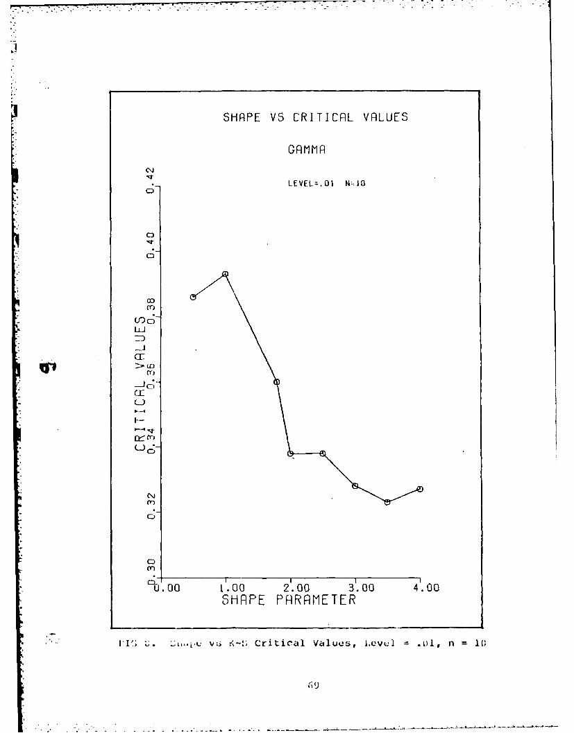
;. Shape vs K-11 Critical Values, Level = .Cl, n =1 69
)" . Sida)e vs K-S Critical Values, Level = .0, n = 15 70
it. Shape vs K-S Critical Values, Level = .01, n = 20 71
11.,aj e vs K-S Critical Values, Level = .1, n = 25 72
12. -;iape vs &",-S Critical Values, Level = .1I, n = 3G 73
13. ;haie v-; K-S Critical Values, Level = .05, n = 5 . 74
1.4. S3ha),e vs 1;-S Critical Values, Level = .05, n = 10 75
15. ,;ijape v: K-S Critical Values, Level = .05, n = 15 76
16. S iaj'e vs K-S Critical Values, Level = .05, n = 20 77
17. .ia,,. vs N-; Critical Values, Level = .05, n = 25 70
I v. .%ntiku vs , Critical Values, Level = .015, n = 30 79
V
* t

19. Shape vs K-S Critical Values, Level = .10, n = 5 . 80
20. Shape vs K-S Critical Values, Level = .10, n = 10 81
21. -hape vs K-S Critical Values, Level = .10, n = 15 82
22. S;haee vs K-S Critical Values, Level = .10, n = 20 33
23. :ihape vs 1.-S Critical Values, Level = .10, n = 25 84
24. Sha,,e vs K-S Critical Values, Level .10, n 30 85
25. Shape vs K-S Critical Values, Level = .15, n = 5 86
26. hape vs K-S Critical Values, Level = .15, n = (' 37
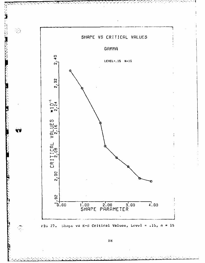
27. St;aipe vs R-S Critical Values, Level = .15, n = 15 8
21. Shape vs K-S Critical Values, Level = .15, n = 20 89
2; . Shnape vs K-S Critical Values, Level = .15, n = 25 90
3o. :*haie vs K-S Critical Values, Level = .15, n = 30 91
31. hape vs K-S Critical Values, Level = .2(, n = 5 92
32. Shaqe vs K-S Critical Values, Level = .20, n = 10 93
33. Shape Vs K-S Critical Values, Level = .20, n = 15 94
34. f-kiche vs K-S Critical Values, Level = .20, n = 20 95
35. Shape vs K-S Critical Values, Level = .20, n = 25 94
36. ;IaLe vs K-S Critical Values, Level = .20, n = 30 97
37, 'hape vs A2 Critical Values, Level = .01, n = 5 99
33. -hape vs A2 Critical Values, Level = .l, n = 10 . IOC
37. Ichape vs A2 Critical Values, Level = .01, n = 15 . 101
4C. Sthape vs A2 Critical Values, Level = .01, n = 20 . 102
41. Shae vs AV Critical Values, Level = .01, n = 25 . 103
42. Shaj.e vs A2 Critical Values, Level .(;I, n = 30 . 104
43. Shape vs A2 Critical Values, Level = .05, n = 5 • 105
44. .,lai L vs A2 Critical Vailues, Level = .o5, n = 1 o G
4%

45. Shape vs A Critical Values, Level = .05, n = 15 . 107I 46. ',iiape vs A2 Critical Values, Level = .05, n = 20 . 108
47. Shape vs A Critical Values, Level = .05, n = 25 . 109
4e . '..iiaile vs A2 Critical Values, Level = .1,5, n = 30 . 110
4(j. 1ihace vs A2 Critical Values, Level = .10, n = 5 . 111
50 . IiapL vs A" Critical Values, Level = io , n = 10 . 112
51. At.ape vs A2 Critical Values, Level = .10, n = 15 . 113
12. J;ia Le V, A2 Critical Values, Level = .10 , n = 20 . 114
53. ;hape vf; A2 Critical Values, Level = .10, n = 25 . 115
S4. Shape vs A2 Critical Values, Level = .10, n = 30 . 116
b5. pha[.e vs A2 Critical Values, Level = .15, n = 5 . 117
,se vs A2 Critical Values, Level = .15, n = 10 . 118
1)7. "hoL,, V:i :. Critical Values, Level = .15, n = 15 . 119
5. i),ape v.; A2 Critical Values, Level = .15, ii = 20 . 120
59. ha pe vs A Critical Values, Level = .15, n = 25 . 121
61:. i;hape vs A2 Critical Values, Level = .15, n = 30 . 122
(61. Thape vs A2 Critical Values, Level = .20, n = 5 . 123
62. SIjat,, vs A2 critical Values, Level = .20, n = 10 . 124
i3. Stia vs A2 Critical Values, Level = .211, n = 15 . 125
-4. Shape vs A2 Critical Values, Level = .20, n = 20 . 126
C5. .- ikj)e vs A2 Critical Values, Level = .20, n = 25 . 127
ka. pi ae vs , 2 Critical Values, Level = .20, n = 30 . 12 3
,7. shape vs , Critical Values, Level = .vl, n = 5 . 13,%)
"8. :;Aaie vs , Critical Values, Level = .(:l, n = I0 . 131
69. Lt;ha e vs : 2 Critical Values, Level = .(11, n = 15 . 132
7C;. , vs t2 Critical Values, Level - .01, n = 20 . 133
vii

• -.:. ijure
71. Shape vs N2 Critical Values, Level = .01, n = 25 . 134
72. Shape vs N2 critical Values, Level = .01, n = 30 . 135
73. Shape vs ItN2 Critical Values, Level = .05, n = 5 . 136
74. Shape vs V.'2 Critical Values, Level = .0 5, n = 10 . 137
75. Shape vs 12 Critical Values, Level = .05, n = 15 . 13876. ',hape v.; Critical values, Level = n = 20 . 1397-. ;fd;V" =, .5, n =2
77. Shape vs w2 Critical Values, Level = .135, n = 25 . 140
75. Shape vs 1.2 Critical Values, Level = .05, n = 30 . 141
79. Shape vs W2 Critical Values, Level = .10, n = 5 . 142
C,. Shape vs t2 Critical Values, Level = .10, n = 10 . 14381. ZhIape vs . Critical Values, Level = .10, n = 15 . 144
82. mae vs t' 2 Critical Values, Level .10, n = 2 . 145
8'3. :hape vs 1.42 Critical Values, Level = .10, n = 25 146
2!4. rsi jat vs , 2 Critical Values, Level = .10, n = 30 . 147
S85. ,Shape vS W 2 Critical Values, Level = .15, n =5 . 146
i. Sha.,e vs 1 2 Critical Values, Level = .15, n = 10 . 149
P7. Shaj~e vs t2 Critical Values, Level = .15, n = 15 . 150
38. .hajLe vs 1.2 Critical Values, Level = .15, n = 20 . 151
f89. Shape vs W2 Critical Values, Level = .15, n = 25 . 152
818. shap1 e vs I,2 Critical Values, Level = .15, n = 30 . 153
19. tihaj,e vs W2 Critical Values, Level = .20, n = 5 . 1540-" ,. 3ihal'o vs 112 Critical Values, Level =.215, n =3i0 153
94. sfia;e vs "Y2 Critical Values, Level = .20, n = 10 . 155
.)3. Shla 1IA! vs 1,- 1 Critical Values, Level =.20, n = 15 . 156
94. 'i:ape vs '\2 Critical Values, Level = .20, n = 20 . 157
5. Tnap~e vs .,2 Critical Values, Level = .20, n = 25 . 158
96. maie vs IN2 Critical Values, Level = .20, n = 30 . 159
viii

List of Table6
Ta t.,e Lage
I xaiaiple: x, F (X) . . 24
C ri Cante r-von Miises o w...2 27
II Andersofl-i)arling A42 e o o . o e o e 27
IV :\oliiocorov-Saiirnov K-S Thesis Critical Values 28
Aollo:oro-&LlirovK-S Lillieforiscritical Values....... ... . . . . . . .2 3
VI i~ovwer Test f~r the Gainna DistributionAl:Gattma DistriDution, K 4ot
Ai: ,nother DiStributionLee fSignificance = .0~5 3( ... .;
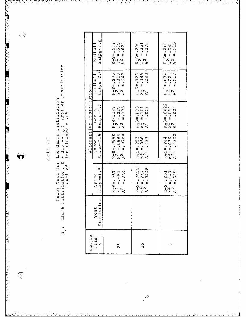
Vii Power Test for the Gaiqma DistributionHo Gamina Distribution, K =1.5
1i itnother DistributionLevel of Significance .05 . . . . . 0 . a 32
Vill Powefr TPest for the Gamma DistributionHO Gamma Distribution, K = 4.01
ii.: Another DistributionLe~vel of significance = .01 o o 34
Ix 1ower 'lest for the Gainia DistributionGamma Disitribution, K = 1.5
I Another DistributionLevel of Significance =., .01 o 36
x Coetticients and R2Values for theh elationships Between the Kolmogorov-"i.irnov Critical Values and the Gai.iinaShape Parameter, 1.03 (.5) 4.V~ . . * . . . . 38
X1 Coefficients and IZ2 Values for theIelationships Between the Anderson-.ir].ingj Critical Values and tlia 3amma
4 'Shape Parameters, lal (o5) 4.V o . . . 40
XITI Cocfficients and k Values for thulelationships between the Cratmer-von
i e.-r .L iL..1 Vcdius aim( tUe GammaShtap~eParameters, 1 .o (o5) 4.0 . . . . . . .42
ix

Pa,Lill
XIII Koluogorov-S:mirnov Shape Parameter = 5 .... 53
XIv Koljiogorov-Smirnov Shape Parameter = 1.0 . . . 53
XV Kolmogorov-Smirnov Shape Parameter = 1.5 . . . 54
iXVI j[ol1ioijorov-Siairnov Shape Parauieter = 2.0 . . . 54
XVII Iolio,jorov-Smirnov shape Parameter = 2.5 . . . 55
xviii i olmojorov-Smirnov Shape Parameter = 3.0 . . . 55
XIX olmogorov-Smirnov Shape Para,:eter = 3.5 . . . 54
X,X Kol1ogorov-Sinirnov Shape Paraiaeter = 4.04 . . . 56
XI Anderson-)arling Shape Parameter = .5 .... 58
Xxii p nderson-Darling Shape Parameter = 1.0 . . . . 58
XxIII Anderson-Darling Shape Parameter = 1.5 . . . . 59
XxIV ihriderson-Darlinj Shape Parameter 2.0 . . . . 59
/ o'lXXV ,\nderson-Darliny Shape Parameter = 2.5 . . . . 60
XXII Aniderson-oarling Shape Parameter = 3.0 . . . . 60
XXVII Anderson-Darling Shape Parameter = 3.5 .... 61
XXVIII Aiderson-Darling Shape Parameter = 4.0 . ... 61
XXIX Cramer-von Mises Shape Parameter = .5 .... 63.. xX Cramer-von Mises Shape Parameter = 1.C .... 43
XxXI Cramer-von Mises Shape Parameter = 1.5 . . . . 64
XXXIl Cramer-von Mises Shape Parameter = 2. .... 64
-.. 1III Crdnhor-von Mises Shape Parameter 2.5 . . . . 65
/ XX iV Cr,.ier-von Mises Shape Parameter = 3.1; . . . . 65
xxxv craimer-von vises Shape Parameter = 3.5 .... 66
AXXVI cru.ier-von Mises Shape Paramcter = 4. 0 . . .
x

A Lst rct
Tihe A nierson-D arl1 miq, Cr a ier-von ~*ises, and(- thc
! olionorov-S.iirnov '7-tetistics are usec' to devulo:' P, now test:
of fit for L~i t!rreo-,:ara.-,eter -yinmc &"istribution wit"I
unknown sihap c;w6 location -arar.eters. "Che critical values
gneratt.c; ,hero obtziine-d, by a i~n~Carlo ; ,roc.2dure. I- or
e a c, v 1uo a t rn ( s;.Ie si 4-e),5--t s a~11u its i*;ere drar.n
frot.,. a jz ta~ulCo w'iiosa shalpe is siec if ied. T I Ie
location an( scale .,roi:.cters are Lasti.-ia-teJ, fromi the data,
an, t;.:- ti 6 rec statistics are calculatc-d )oe, on thc esti-
mated distribution. The simulation was, preformed for sai-. 1Je
sizas n S 5±tl... 3(4- and sha~ 1-arauietprs, : 5 7r
isinyj gammna distributions for siia:,e ccual to 1.5 and
't~,the i~ower of each test is investigat:ed ag~ainst ten
alternative cistributions for savi;'le sizes n S 5, 15, and
30. In general both the \nderson-Darling and the Cramer-von
!,ises. tests are more powerful than the ''o1rogorov-Sinirncv
test. Excevt for the case whiere the altLernative di stri Lu-
Lion is~ lc-Jrr:' al, ttie Crainir-voi. ;1,ises test is the iniost
iowerful test.
'.'he functiona~l reliticnisliip bctween tne critical vaIlues
of the Anderson-Earlin,., Craier-von 'uises, and X<oli,ogorov-
Smirnov is also exaiiinad. 1\ critical value for a ij)4-C
* paraiiieter between 1.5 and -~which is not included in t~ie-
relationship.
xi

5 A ;AUDIED Li) tOLmiGGOkOV-SP IR(NOV, CkAM~ER-
VMi4 m~ISiS ANE, AN[WR5014I-DARLING TEST
ei Ok Tlii (CAM~MA DI STRILA0iION 1-;ITh
LJNRNO1Mq LOCA'iION AND SCALF:
1 . Introuction
Curren~tly the U.S. Air Force is placing~ m~ore and more
N eimipasis on systeim, availability, wiaintainability,' and reli-
ability, both in research and development and in day to day
operations. Of4 particular importance to the Air Force is
the atbility to predict time-to-failure of equipment.
.tudies ini probability and statistics have increased under-
* -standirU ot S-Oie Key probability distributions used in pre-
dictin; tirve-to-f a ilure. Among the most commonly used
coritirnuou . distributions in this area are the beta, gamma,
exPoniriunial, 'eihull, and logjnormal distributions.
utt,21 il, Lhese studies, analysts are confronted with
the probltem of testing agreement between probability theory
and ictu 41 observat ions. In other words, given n observa-
tions of soize variable, say ti ime-to-f ai lure, the problem is
Lo tind out it it can be recjarded as a random variable
fizcvinj a cji'v'GJ probability distrib~ution. The general
ai-p~ruucl to tke solution of this pjrobleia is known as the
yoodie~;-uftutst. In more precise terms let x 'x 2 .x~
be it ran,_Aoti :iatmole. Then a stateiient of the joodness-of-fit
* test i.:

H A: lI(X) v, W~1 x
where ix) is the actual distribution function of x and
11,,(x) is the hypothesized distribution function.
2

a kroun d
Yewo co~imunl1y used 9 oodne ss-o f- f it te st s a re the Ch ii-
-;.,uare ttest aind the Kolrioyorov-Sinirnov test. The Chi-sqjuare
te-It cottilret; observed frequkencies with exi.ected frequencies
ot tHLu JLyottiesiized distribution. It is restricted to lar-jo
1,. 1L;L-..Jrxmt 25 or gjreater (:1:73). The K\oliiocjorov-
..uiirnov (-)tuSL c0Lmparces cui,iulative trequencies between
Ihe ZCLucal ~~l ujiiw - a step function, agdiinst orrespond-
in ..i~~~usin~j tin(- hypothiesized cuildulativu distribution
junction. Oiie I(-S test can be used [or laryc or small
tdifijlLS; ihovvever, it is restricted to distributions which
kj illy sj:peci1ied. Ii. N1. Lilliefors developed a goodness-
ot-l1i t test Cor the norwal (19), and exponent ial d istr ibu-
t iu o2~ ia .ji ich can Ibv used for s~ia 11 samples where thle
~.~r~etersiust be estii mated f rom the sai.iple data. lvhen
~uri~cer5are estimated froii saiipic data, the test is said
to !,L a modified test.
I-ollowini1 Lilliefors' technijue, several other modified
tLe:,Ls have been documented. u. Cortes developed a mrodi fied
:ul ~J(Jv!.,ri~vLest for thle three-paramtner Vveibull and
*joVInlaa diLstributions (5). J. Bush expanded the .joodness-of-
lit te!SLt or ue t'.ibull to include tile i,oditied Crafier-von
S V:; i. ti~d .%riuerson-Iarlinj ( 2) tu.;tsI (30i). The modi-
Lie(, ..uiiujuruv- b3i-oirnuv, Cr~;dier-von *l1.e, nu Anderson-
;,cirlii i tu.-L_5 have also been done for thie uni form, normall ,
La 1.,x~L:., Lcx, oirientiu 1 and Cauviiy rdi~tr iiutions (11). In 1973
*.n, cictier , and iLerticjJrc!.ijneuI two new tcest statistics
3

*called the L andI S statistics. The L and S test statistics
were used to develop a goodness-of-fit test for the two
paraiieer eibll ithunkownparameters (22).
In l1"l , outrouvelis and rKellerraeier introduced a
coodncss-of-fit test based on the empirical chacteristic
function -when the parameters maust be estimated (17). This
tust statistic could be used as an alternative to the F:DFE
statistic if the characteristic function is more easily
ut LeCrmint.:,, than the distribution function.
tEhm irical iistribution Function *Stcatistics
A jererzal class of statistics used for the goodness-of-
lit tLeStS is called empirical distribution function (LDF)
statistics. wistorically EMDi statistics have been used in
cases where the parameters are either known or unknown. In
mrost instances EDF' statistics are easily calculated and are
competitivu in termns of power. This class ot statistics is
base] on a cosmparison between the cumulative distribution
function, F(x), and the empirical cumulative distribution
Eunction ,;,(X) defined as
no. of xSn W = --
n()
'he test procedure is summarized as follows: given a sample
Lrm somum jopulation, the ! DI te!sts, rejo~ct i(,:F(x)= (x
wheni the ditterence between i,,1,(x) and Sn(x) is largje. liere
L.*,(x) iLi tku hylpothusized distribution. In jeneral, EOF
tests are valid when the distribution is fully specified.
* iouwevur, 11ivid and Johnson showed that the aistrioution oi
4

S,'an L. statistic depends only on the functional form of the
distribution and not on the unknown parameters when the
estin: ated parameters are location and scale (6). It is this
principle that permits us to generate valid critical value
tables for the gaim ,a distribution which dePend only on the
shape pjarar:ieter and sample size.
It is imL portant to note that this thesis uses a modi-
fied form of the EDF statistic, because the cumulative
distriuution is not fully specified. An estimated distribu-
tion function is used whose parameters are derived from the
observed sa,.Iple.£2_. 5"_ojorov-S-.iirnov Statistic
.The Kolnogorov-Smirnov (K-S) statistic is defined as
the absolute value of the difference between F(x) and Sn(x)
or,
,'.D = I F(x) S Sn l -~ (2)
In usinj the K-.; statistic for the goodness-of-fit test, we
are intcerested in the greatest absolute difference between
i(x) and I;n(x) (2). Therefore the test statistic is
sP IFl(X)-Sn(X)I (3)
h'e Amderson-Darlinrj Statistic
It i:; known that goodness-of-fit tests which use actual
observation:; without grouping are sensitive to discrepancies
at thu tails of the distribution rather than near the nedian
(1!:2). The Anderson-Darling test statistic overcomes this
problemm by accentuating the values of Sn(X) - F(x) where the
"- test statisLic is desired to have sensitivity. More
5

specifically, tne Anderson-Darling statistic is based on a
weighted average of the squared discrepancy, (i.e. [Sn(x) -
F (x)1 2 weijhted by *(F(x)) or
An2 = nf[Sn(xl-F(xl]2 (4)Fx) dF(x) (4)
where
* (;(x)) = [F(x) " (1-F(x))] 1 . (5)
Using the computational form
nAn -n - . E12j-l)[in F(xj) + in (l-Fnj+l)], (6),. n j=1
the test procedure is as follows:
1) Let Xl<X 2 <_..._Xn be n observations in the sample.
2) Coi~q.ut : An2
3) If An 2 is too large, the hypothesis is to be rejected.
The Cramfur-von Mises statistic
The Cramiier-von mises statistic is a special case of the
A 2 with ['(x)] = 1 and is written asiiSn2 = M (X) - F(x)] 2 dx. (7)
This test procedure is the same as outlined for the
Anderson-Darling goodness-of-fit test (26). The computa-
tiurnal form used in this case would be
nV[i x ) = 21 (8).. 'n2 12n j=l 2n
!i L, ~~robl1em,___/ ;ta tement
Few joodness-of-fit tests are available to perform on
sample data when the parameters of the distribution are not
known. As mentioned earlier, Lilliefors developed a test
" for thu unspecified exponential and normal. Also, bush
6
........ ........."..".......".... ... --..... .. ,

. -. generated a set of critical values for the Weibull with
unspecified scale and location parameters (3). There still
exists the need to develop a valid goodness-of-fit test for
the janiia density function when the scale and location
paraieturs are unknown.
The purlpuse of this research is to develop a goodness-
of -fit test for the 3 parameter gamma when the scale and
location parameters must be estimated from the sample data.
This involves generating a table of critical values based on
the sample size and the shape parameter. The accuracy of
the critical values must be sufficient enough so that data,
sai. pled from other populations are rejected.
.,I c tives
This thesis has the following objectives:
1) iTo generate and document the Anderson-Darling, Cramer-
von ,.ises, and the Kolmogorov-Sirnov rejection tables
[or time three paramqter gaitima distribution where the
.calu and location parameters are unknown.
2) To conduct a power comparison between the Anderson-
iarlij., Cramer-von Mises, and Kolmogorov-Smirnov
goodness-ot-fit tests.
3) To investigate the possibilities of a functional
4| relationship between the shape parameter and the
critical vdlues in objective one.
7
7

-. ., - .. .,. ,,, ,-.. ..- - ..- . --. -
: I• The , Di;tribution
i'lhe jan.,u density function is usefuil in reliability and
,: d, intainability theory. It also has ap.plications in the
natural .;ciences. If the randoi. variable x is jwuia distri-
buted tinun the probability density furction taKes the form:
f(x) = (( <(ex (X)), (9)r(K) e
", , > 0; x> c > .
" .'iece are three parameters which Lipecify the gamma. 0 is
thu scale -;araiieter; K is the shape parahieter, and c, the
lucation pardieter.
Thu cort ;lexity and versatility of the jamia distribu-
tioo can ou observed by examininyj the graphs of the distri-
5ution for vairious; values of the shape and scale paraneters.
k itj re 1, show:i jrapjhs of the standardized gawma (i.e., c-0,
=I) tor and 5 (7:370i). isVhen <=1, the gamma is
the exponential. Also, it is interestinj to note that when
is l;. thmi one, the jamma closely resetitbles the exponen-
t i, .1 i~ Ar i but io||.
,..Lu, 1 ijure lb shows that for larje K (K=5f), the
a r0!;C!.Ilcl..s the norral distribution. eigure 2 illus-
I. rd tii intIluIcr e of on tir -jr dh of tnc jaAi.ma. here
w(. UL -=. n =2 aria s~etci the cjraj~hs fot 0 =1/3, 1/2, 1
a, ;.' (7:371).i.
. .. .

.3
.07
1.0
[Ic; 1. raphs of the standard a)amioa density function for(aK .5,2,3,4 5 and (b) t,=50

.2. eti
VI G 2. cralliis of the standard qainina density function forc 0 (, K =2 and O= 1/3, 112, 1, and 2.

"A ),lication ot the Gamma Vensit Function
The 'Jalilbaa distribution is otten used in reliability
theory to represent the distribution of the time between
lailures of a system. Assume, for example, that a system is
*;ade up ot r coiiponents, all of which must fail for the
-, - system to fail. furthermore, assume that the time to fail-
ure x i of each component is independent and exponentially
distLriuteS. Then the time to system failure Y =X 1 + X2 +
+ Xr is jamma distributed (7:369).
In clueueing theory, the random variable T follows a
juo!lia distribution, where T = X + X 2 + ... X is the total
ti.,e to -service K customers assuming that the time of
service of each customer is independent and exponentially
* distributed.
Tije twio cases described can be modeled as a special
c 0Z 01 theL! jamma known as the Erlanj distribution and
uxi.re:;sud as:
Kf (t) t ) .tK-I e-_ t' t>0. (I(;)
A random variable having a ygannia distribution has also
t,een used to represent or measure the occurrence of physical
"liino meii . [-or examiple, Slack and ,rubein (1955)
"(d,:eonstrat:d that the mean value x of radioactivity (alpharic~le per Linute) witrin a sample of Pennsylvania shale
followe,j a ..,waistrihution (7:37(0).
4"
L1
I + . . . I • ; ,i

Tfhis chapter presents the Monte Carlo simulation proce-
dure used in jenerating the critical value tables for the
rioJ i fied :"oliiojorov-Smirnov, Crarier-von ivises, and Anderson-
;i r I iii~j t uiL:;. The L)rocL'duru 1:S outi inc~ L.;in~J the flowi
citir t in I- iju re 3. Secondly, an outl ine of the power coin-
pari1 on aimonlj the thrue tgoodness-of-f it tebts is given.
Thirdly, a discussion of the analysis of the functional
relationship between the shape parameter and critical values
is presenteo for each of the test statistics.
i-ionLtC Carlo Simnulation Procedure
The followingj procedure is used to yenerate the criti-
cal value tables for the modified goodness-of-fit tests. As
weuntioned earlier Figure 3 presents these steps in flow
chart formiat.
1) For a fixed sample size n and tixed shape paramieter ;
n standard randood gamma deviates are generated using a
computur subroutine. The standard gammna deviates are
converted to random deviates with location parameter C
I,;~ and scale parameter 0= 1.
2) The ni randomr deviates are ordered, x ( 1 )' X( 2 )1
X(n
43) Th'le ordlered random deviates are used to
eLtiiiate the maximuai likelihood scale and
location parameters.
a 12

ST~AR T
Generate Random Step 1.;ammca leviates
Order iandom Step 2Ca6%i; a ;Jeviates
E'stimate Location Step 3and Scale Parameter
Determaine Hypothesized Step 4,:- Distribution Function F(x)
o 0 Calculate A2 , W2 or Step 5: I1*.-,S Statistic
.eteriaine the 80th, Step 6:-.-3 5th, 90Jth, 95th
aaij v.bth iercentilu
LW
FIG 3. Flow chart
, 1 3

4) The eLtimated scale and location parameters and fixed
.Shape parameter are used to deterj:iine the hypothesized
distribution function F(x).
5) The test statistic is calculated using equations three,
six, and eight, for the modified 1"olriojorov-Smirnov,
Anderson-Darling, and Cramer-von iiises tests respec-
tively.
6) tepA s one through five are repeated 5000 times.-
7) 'i'he value of each statistic are ordered in ascending
or, er and the 80th, 85th, 90th, 95th and 99th percen-
tiles are used as the critical values of the test.
IteneratiorL of the Three Parameter Gamma Deviates
ior the gamma distribution function, there is no closed
forsj,, for which we could obtain an inverse; however algo-
ritL, is are available which can be used to generate random
garluaa dleviates. The IMiSL subroutine GGjvtAR is used to gener-
a e standard ganma deviates in this thesis. These standard
duviate; are converted to deviates having location C = 10
and scale 0= 1. This is done by using tne transformation
z = " x + C ()
where x represents a standard random deviate. This trans-
oriat ion i nade to avoid a problem with the parameter
L!;ti;ating routine. Further discussion on this matter is
prosented iik tne following section.
,"a.<1imu;d lLikulihood Lstimates for the Gaiimia 1,arameters
ihe procedure used to calculate the maximum likelihood
es ti.ctes Lor jamma parameters was developed by Harter and
14

Moore (12). Their analysis involves the derivation of the
maximum likelihood estimators and includes an iterative
method for solving the simultaneous equations. To derive
the 1aaximum likelihood e'.uations we begin with the jamma
density function with location parabieter C>_, scale param-
uter 9 , anu sha,e i:arameter K:i:-.[(xc, Ohl) = 1 "A-c k- u x _f- _c
.f- x , -x, (12)
KTlie l iilinood function of the order statistics xl, X2,..xn
ot a l of size n is
L 1 )n lt 'k-1 exp x=1 (13)
.e wisih to Iind the values of 9, K, and C which riaximize L.
Irv Thi-; is done by taking the natural 1',garithm of L, and
sutting tlhe ,aLtial derivatives with respect to the three
pa,iiraeters ceIual to zero and solving the three simultaneous
equations. Tfe partial derivatives are shown here:
::: i ,L n, k x i- c.'r-L . "k + - (14)
i=l 09
c)in L n. -nln9 + ln(xi-c)_ n "A-K) 1 (15)
-. i=l
"-1-nT = (l ) (xi-c)-' + n i,* (1-K) + n1(
IL s3tould be noted that because ol a limitation of the
hart-r an(,+ ";oore subroutine, it is not possihle to estimate
) . tilL iaramiet ers when tne -gamma deviates are ,jenera'Led with
location C = 0:. In the event that gamma deviates are
15(

generated with C o ~, it is poss~ible to obtain negative
estimates for the parameters. The subroutine imaps these
negative estimates onto zero. Thus, C' ind *will not retain
the invariant property which is needed for these tests to be
V'11idj. In addition, the iterative techniqjue used in the
iarter and [foore subroutine does not work for the special
case whien the shape paraimiter is set to one. because the
caiais aim exponential ditribtion when the shape param-
etur is e. 1 ual to one, we can use the tm,'&ximum likelihood
estim~ators of the location and scale pjarai~ieters for the
ux1 orintil. ierefore, setting K eqjual to one and solving
uutions 13 anid 1'&: we obtain
C = (17)
anu
e=A Xi * - 1) (18)
-erivi the iyothesized Distribution lFunction F (x)
Th~e jidaximuia likelihood estimnates for the location and
scal I raiiw-rs and the fie hpeprntr deter ineI
Wx. Obtainincj a numerical value f or Fix) req4uires an
inteLjrai calculation; this calculatioii was done using the
1;i.';L suhroutine MiDCAM (13). ivDGAM calculates time probabil-
iLy tliat a railoni variable x from a standard 'jamma distribu-
to(i.c., C banid O= 1) is less tnan or equal to x. 'I'o
t r"An;iori t.-ic -!Viates, yi, trom a joneral ized gamiira di stri-
buit jog, i nt-o !tandari yamiiia deviates we use
4 aC

The details ol this transforimation are provided in Cortes
• (5: 17).
Poa.r C ci,;. l [ ition
von uIsen, d t.nderson-Dar]inj tests -ire compared for ten
alternative distrioutions. Sauiiples of sizes equal to five,
15, ,i nc 25 are drawn from tte followirt selected
.1i st r i h, t ions :
1) G , shiape equals 1.5
2) Gauunia, shape equals 2.5
3) Gawwa, snape equals 4.0
4) .cibull, shape equals 2.0
') ,ci,uIu , share equals 3.1'
C.) [jorial (10{,1)
7) beta (j = i, q 2)
P) b!eta (j, = 2, q = 2)%.I 9) Lo-jnorcial (, I , w 0 )
lo() Lojnormal ()- 2, w 0)
Thezcs, distributions are tested according to:
- .;: The samjle variates follow a gamiia distribution
havinj shape parameter K.
.. ,, The samaple variates follow some other distribution.
'lie 1,owt-r i nvustijation was conducted under two null hypoth-
"z-eb, one tor shape parameter, : 1.5, the othur for shape
L. ..cL.r, r: = 4.r0 . h rac n ot.: devi,tes for the above,iLurnative distributions were enerated using IMSL
sulroutiins.
17
-- - .... . -
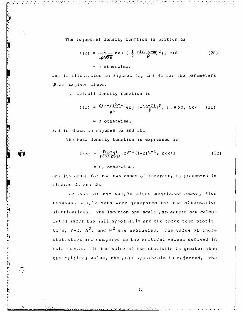
Tihe lojnor,4al density tunction is written as
1- Iin. x-w ] 2x x ( [), (>O (20 )t (x) ... L. ex, p- I2.~Z),((
1= otherwise.
I id j i., ill u,Lz,.t in [ijuy es 4a, aiv! lb for the ,arameters
p W -j. JiVn above.
, n.ull .cnsity unction is
x ): X S) I ex1 , ]K , 9 >( C. x (21), exi 0
= otherwise.
and i,; shown in liyures 5a and 5b.
'ihleta density function is expressed as
f~) £~)xpll-x),i-, l:<X<l (22)
= 0, otherwise.
arn,, iLt jra i.1 for the two cases of interes;t, is presented in
I i,,Ur C )d and Cb.
, (r each oL the Saimple Si;es 11eritioned above, five
thou~A~ni ~~uAL l;CL ets were generated tor the alternative
ui~triuUciu . The location and scale !arametert are calcu-
-l ,ed rmer the null hyp othesis and tlie three test statis-
Lic, ]:-.;, A 2 I and N2 arv evaluated. ilhe value of these
stiLizLi-'S aL% cum|pared to tne critical values derived in
S tIhi t;i,:ii:.. IL the value of the statLitic is greater than
the critic ,l value, the iiull hipothesis is rejected. The
11

Ad..
Fl (G 4 a Lo~jnorinal FIG 4b. Lognormalw 0. p=1 w0. p=2.
I- 12i 5a. Ueibul1, K =3. 5T 9b. Iveibu11, K =2.11.
1. C=0. ei 0.
19

7,4
I C3 (I. EA 1eta, FIG 5b. beta,p=1. q=1. p =2. q =2

total number of rejections are counted. The power is the
total number of rejections divided by the number of trials,
Determininj the Critical Values
t. repjeatiny steps one throujh five 5[0 tiles as shown
in thu flow chart in Figure 7, 50 .,[ vAlucs for K-S, A 2 , and
1 2 trt calculated. These critical values are ordered and
the 83jth, 85ti, 90th, 95th, and 99th percentile are used as
Lhe criticaL values of tne tests.
''hlu voiraLditer pro~jrams used in this thiesis are Presented
in iqA enrdix C.
21

IV. Use of Tables
In this cha[pter a set of steps is jiven which is used
to jperfurk~ii z;joodness-of-fit test by appjlyingJ any of thle
LlhrLu c te:.ts eveloped in tiiis thesis. Als~o, an example
i1Lustr-tiCiutAj Andersun-!,-:rlinj LesL is presented.
Thu.. lolow~in~j steps are use(d to j erforii a goodness-of-
L tet:
1)i)eteri~iine tile shalpe paraireter, 1K, and the desired level
2) 1 rw~i thu d-ata to be tusted, calculate tile i~iax imum
I iK e Iihood est ima to rs f or the location and so-ale
3) L'roit the ai,;rapriate- table, select the critical value,
dcorrespondin(I to a ,the sample size n, and shiaje
4) JUi~-j the !w.x1ilauj~ likelihood estif-1-ators, determine tile
es3timated hypothesized distribution, arid use equation
tlirveu, six, or eiyjht to calculate the !oliaocorov-
.nirrnov, Anderson-Darling, or Crari-r-von Nises test
,itatis;tic respectively.
It) [Like value obtained in step fuur is jreater than tile,
critical value tound in ster) three, then reject tile
kL1.o~~sicd is-tribution. IL it is siiialler than thle
critical value, ttlen thu hly~otihesizudI distribution can
nlot, &LCuCteJ.
22

x ai't k' C
The time between failures of a particular subsystenm of
a radar system is believed to be distributed according to a
.jaitia distribution with shae parameter equal to 3.0. A
test .cimineer recorded the following tii;es between failures
o0 that sub!;ystem: 11.1, I(0.6, 10.4, 13.0, 1 1.3, 10.5,
1t.C, II:.9, i0.(, 10.8 days.
,. rioditeid AnderSon-Darling test at a .05 level of
Ss ijri i i'alice is performed usint4 the critic.uI values in this
triesi;. The proulem can be stated as a test of hypothusis,
tlat is,
i U: The distribution is gamma (shape = 3.0).
iA: The sawple comes from another distribution.
Lirst, tie level of significance a, and shape parameter K,
have been ,deteriained to be .05 and 3.o0 respectively.
er;UI', Lh tiiaxlmuiI likelihood estiinators calculated usiny
the Htarter ard ',oore subroutine are C = 9.319 znd 9 = .U2(.
reuxt, th. critical value from Table XXVI is .8415. The
hiypothesized distribution is completely deterwined by the
tiXUL.' snape paramieter and the estimated location and scale
.aramuters; these values are presented in Table I. The
value oi: the Anderson-Darling statistic is A2 = 1.7342.
,incc 1.7342 is (jruater than .""415, the null hypothesis is
roj-ected. Therefore, the conclusion is that the sampjle of
tiiiu betweoun failures comes from soie othier distrLC 'ion.
23

'±AL LL I
i t x L(x)
1 10.4 .1532 10.5 .1633 i1.6 .2034 10.6 .2115 10.8 .2696 10 . 9 .3 07 11.1 .3846 11.3 .4329 13.0 .822
l0 18.6 .999
42
| 24

V. Discussion oL the i<esults-
Tkiis chapter presents the results obtained with respect to
the objectives stated in chapter 1. These objectives were to
develop modified Kolm~oorov-Smirnov, iAnderson-uarling, and
Cr,-Iite[-VOn i-isus tes~ts for the qartm&wz ans,' coiiipare their
o w ers. Also included was an investigation of the relation-
si ji Luctwien tie cri tical values of each test and he
pa raw.et !r s. Included with these results is a report on the
val1 'latioii of the coni,,uter progjrams used in this thesis.
ire :;Ltc.Lrion of ttue I~ln~rvSnroCramer-von Mises,
andi Aneron-jrin Tables of Critical Values
The tables of critical values for tthe modified K-S, A2 ,
aa * 2 tust , are presented in Append ices A, 6, and C,
'-Alil theu Slape paraitetur is fixed, both the K-S3 and A2
critic.,il values are decreasing as the sai~iple size increases.
Tile rate- UL dlecrease is siialler as n increases; this is an
ir~dic'atiori that the critical values appear to be convergingj
for larcju siml szs The Cram-,er-von :iises critical
values, ol 'lhe other hand, are increasing with respect to
thte saii, 1 le size. Again, the rate of increase is smaller for
LaIr~1er valties of n, indicating that the critical values are
convor jiIn tor ]care sam-,ple sizes.
ILt shouldib notedJ that becauIsO the critical values are
Je.r ivc>i LIiruj~jli Monte Carlo imul at ions, the values are iiot
error frue and toat ttic,aimount of error decreasus as the
nui,,&ur o1 Lriu.1s increases (25). The 5000, repetitions used
25

77 7
in this thesis was a practical compromise based on computer
time required and accuracy desired.
L£- Luter L) h Validation
he computer trograis are verified by generating crit-
ical values for the exponential distribution with unknown
Wean. 'hi.; is done by generatiny gamma deviates with shape
[arameter equal to one, fixing the location parameter at
sume arbitrary value, and estimating only the scale
parameter
'I'le critical values are calculated for sample sizes n =
5, lo, 2U, and 30. The critical values from the Anderson-
Darlinj and Cramer-von Piises statistics are modified using
expressions (23) and (24) derived by Stephens (27):
~A 2 (1 + 1 5 _ 5)(23)n n2
'IN2 1i + ._-1 ). (24)n
*T1i e comiuted critical values are compared to those
calculated by Stephens (27) for significance levels .15,
S'hiie critical values calculated for the Kolmogorov-Smirnov
statistic for the exponential are compared ditectly to those
c(erivuld by Lilli',fors (2 ). The critical values which are
derived from the programs in this thesis are presented in
Ti,le IV and can be corompared to Lilliefors results in Table
IV .
''ic critical values for the Kolmogorov-Swirnov statis-
tic cumipared very well to thi. Lilliefors values. The
26

crainer-von miesW
2(1 + .16/n) Stephen'S1-x ICr itical
n= r=l(j n=20 f iz30 values
S .42.149 .148 .1523 .149.177 .7 .174 .17,r .171
.5 .22C .21 .221 .221 .224
.9 .341 .332 .335 .325 .337
i\nd(rson-Darlirvlj A~
I~ ( + 1 .5/n - 5/n-) St e Ph en s1-x:- Critical
nn= I n=20 n=3.I Values
.41.992 .5 61.922
(5 1 ."17 1. 3 81 1.37G 1.372 1.341
0 2.7t; 2.219 2.077 1.974 1.957
27

TABLE IV
i Kolmogorov-Snirnov-__Thesis Critical Values
1- n=5 n= 1 n=20 n=30
.85 .378 .276 .19.) .166.401 .295 .214 .178
5 .447 .328 .235 .193
.99 .531 .384 .27t; .232
TA uL L V
Kolmogorov-Smirnov K-SLilliefors Critical Values
I- n= 5 n=lf) n=20i n=30
k.5 .382 .277 .199 .164.9'r .4C6 .295 .212 .174.95 .442 .325 .234 .192
.99 .5o4 .3803 .278 .226
28

jreatest deviation occurs for n = 5 at significan'ce level
.0l. The Cramer-von Mises values generated are very close
to Stephens values with the greatest deviation being 3.6%
for n = 3(o and significance level at .0I. There was also a
ood matcl between the Anderson-Darlin,. values, with ilost
:.eviations 1,etween 3% ant 4%; however the 'jreatest deviation
i 13.4, tor n i0 and signiticance level .il.
v'ower .Irivest i.jat ion
,m power coij. arison is made between the iKolmogorov-
Sinirriov, i\nder son-Darling, and Cramer-von Plises goodness-of-
fit t*.x ts cieveloped in this thesis. The gamma distribution
4ith sha~ie parameters equal to 1.5 and 4.0 were both used
against the alternative distributions listed in chapter III.
5).,a l sizes five, 15, and 25 were used in the power studies
at botil an a-level of .0,5 and .01.
T'ah1,es VI through XIII show the results of the power
co,;j.ar i:tons tor a-levels .05 and .(I. 'hen the null hypotl-
esis is truu, the power meets the claimed level of signifi-
canc,_ to the second decimal place in most cases. For all
test-i tiie power is low for sample sizes equal to five. In
tact, in ;,iost cases for n = 5 the power is nearly equal to
the s -jnificance of the test, indicating that the goodness-
of-tit test has no practical use for very snall sample
. z e- s.
Iii nuerly all cases, the power:; of the Cramer-von Mises
and/or ,nuersor,-Darlinq are qreater than Kolmogorov-Smirnov
test!;. Fased on this study, the lattLr test would not be
29
• • ~~ ~~~~~~~. t " " " - ' "m . .. . . . . | • '

a.) n) U) .0(
J: (N C1 -lC4I C 14
-4%X4lC
0- CN)0 C"I C-
Qa *u ) u . .r 9 K 9I U) U
4J ) ( UI IiNN C14 ICNCN
r-, V.% sCt
.J
II r C 4 I C
U44 1'. 9 9
'14 .01 U'
r3 r- LI LO
-4 a) 1. CIN CNc r-r-r -4 '.-
.1 rC l)U) zj)C AC'J I IN CN 1IC4 C14
C) ~ .- 4
~4-4 -oLAI* rN.. ['LJ-
Li 0~l '-~~CN .~r30

CN CL CNNCJ 1-4 P%
11 U) -4 , -4 Ur) I -r
41 ZD rs Us1 C.)
-4. CoN I-:) 11 1 1 I II In I
4-j (N --j -i a
*~ 0 0I ICN( IC 4ICJ
(C IN) I- r N l 1
4:3 4. Ifri% oM V'
.4 izn- w0 3) Ch 0 0 6
L11 (I U); U) If C) Oil 1 4I 14 C'4 I~ C
4J -4-c..
w4 C14 k- N w.llL)I
5 1)) r- mcu-rI-
o t :+- 4.oQ 0* C00 0 00
Hr- I 11 II H 1 IIc" U A Ur.I )
'-4 0~ it' C- C-4C' N N
... 4 U.4 %.7
[(N (N I(4 C') 1(N4 (
4LJ -J
I(NC LCC ICi'
4. -4 C1 r-' r c -v C%4 C1-
-4 11 L4
-~~~ :iI N'1'~J]..- Ci.4 C%4 C14 I I I I I
r-- :0. ICNJC- CNC'-3 .4 4-;4.) C N r , .
Ll. . LA rf -4 n'. u z:
4.) 0 . 0 0
U-) '40 '-4 X: 1 ,4 N -4 N C%4
C.; 11 LAj c -W rC'1
-4. 4 4, * 3')
-0 Z ) 1 I NCN IC',C14
t.) 4n'44
'44 -0 LA w
4J ~ ~ ~ ~ L r- %V li AL ~ A~jLu-- C.) IIr L" J ;
11 11 If 1 1 1 f 14. t Ln cr In
Ir'CN C IrCN 1C1
a) - --
o J
U) W.
-44-'n
32

.-) T LO k%, Ii N (n N 0i LiJ(1) s e . ** 0 . 00*ca 11 If it 11 11 1 it It
r U)J CN C14
.9-4lwr-
kc.- %4L. r-4 -ti C40 c 14i
0n Z- C. U
A-j C" - U) )UW, 0 (NI I S.N NII
: -j 44J I . r c- 04
.4 Q-0 a 0 "
it2 it I N it i it t I
C) l 1) 0If N I C- N IC s
(14 NQ .n r- 1w IN *
0o -, )u) ONt - %C)~-; CN IN m)1 Ir-4N -ICJ N
99- -- 4C-) (o= 0t 11NIC NCII
4-1 >)f
4. L'44
) t
4j0
LIA Ln LA
33

I ~ ~ ~ -N '4cNC:
C~ C14 m c
I N
0
4-1 CO
4J 4.1 U U)A
UI N.. INN IC'.4NNN
4.) a) r- U' N, k
* ~ ~ 1 C- C.E * . * *
oi null-4 11 It11
4j gI -91 <.. l' 'jgcj ~ g-i
44 u
C-4 C1 C1 Nt Cl * 4.l-if
4-4.
LO LO U))
C * o (A~)~'34

It 1
' N Ir U
4J ("(i C.
4 J r c 0>&n flhJ Ln wr- c cj:3i CN r- f- mM n -1 U
Ca . . Li Z .
4~J C:(2(A0 11 C IC'4\ IC4(N I(CN
-4
44.2
4.) IJ 0 1 '4r- C' \
-4 >,4 3* * *
-4..4
43 M-4 C__ V___e__) ) ,
I (0) CN fn.- m C- 7
-n r- Eli2
-47Oi C'4 CN 1 (14CN (
.4I-1~ --4 r--O O
Cno- %r -l: k:-4.-V) -
U) Ci)U
o 0) >
A-- U)4 -- 1 C C'4 N--4
LI) Lo-
1-4 a2)
If) U) WI
J!(

1± 0.3 9 v 9.. 9N 9 (1991- 1 In Nr uI a.) C...)I N
IC'J~I 11 ItC IN '
0
'- 9 C C14 (N M, k I)N CN3~ 14CJ -4 C,4 C. ff (n~ IN.
F- w ± m 9 * * 9
U, ~ ~ . CNC1 .u 1
4J4
(14 (.N CIS) N C
w) Nl N) IN IN 1- n c- I(CQ
2 :G 4 .0 0a.
<~ C; (I u) l
CN N Ii-, N c'.J.- N
~~~0 In-' ~
tD4J 0 0(
i) If
-r-" (N I I N 1ICN
S4U)
4-. 1
U) V)
~~.j44-1
U) ) U)4'))) (N -

0) * j k . . Ci t . .
C'd C-1 C)) C.;C-C
0 0______ 0 0 0 0 * 0 0
- &l 11 11 1. C'J 11 . '.1 C'. 1,
i)C- U~ tr C* I I i I I
Cd 0 I4J I IJIC J 'C'
, ~ ~ C' ...- 41
*.I %L) G'4~
0 ''C, :", '0' 1% .. .' c- .
U l U) 0.1 0 11 I C N gN JIC'I) CN
II .- * > 34
oU -4 c.4 CD
%r U a44' 4.1 0 o
04 (1~4 '44 I;' Ci) CN1C)
-44O~ lC.C' ko GoN Vo C :
wV U., %D. - n rlC 4C
o o o 6 o o
V) U )
Uu)
(.37

CNA
m -1 ON 00 U)r-4 N1 cr-4- '.D
41'
4-1 1 - 1) ON C% VI.Z
-~k - C; t- CN
U) -
cli r~ U r-ONA
U) 0
-A -
.34 (U- ON A
..-- t;r c$'0L C-4 U'). m 0)
u. 0
C-) CV) C.; N
0
%TP -4
C0) (44~.
"-4-4
~t3OL~ - ~ N U'

u I
U3 r'. LI k
LA L
CN w
r, C..) 0) C'
* C' C. ONl r-4
-1 LA 0' NN
ko %P ~ 4r~-
uLA
-4
Ao >
* 39

V) U-1C)
r- (NA N t;;U.) (N '*
N I-N (N 'C4
Li) ClSi m0 SC",
LC')
CaN
4
* 0
(1) ;J-4 m
>l C C
*4 0

LAA
-4 (
Q~ (N -N
U''3
r3-'
L;) C) %D kZA t.0~C
ON CA
RIP C. r-4. '
m '.0 C).4 .-4:3 Ln LO 'A1 (C n'
44
* N ((nN'A
AA >)C
0)-Ira
* 41

6
41 -4
*i Cl ) Cl) V C4 (I 'j
-Clfl C4 fn.. C .
Li)
4 J k*f 61 Ca. N- Ca ~I-~. Cl CO -1J ON 1.- -i 1-4 C. -44 (I.- (
Cl) 'Cl
..-4 (01~ C
E--
-41 -4. a). .-4 LCL.k)) N
NN 0. W. 4 .
4.)
1)0
> (3 CL .~U ~ Uc LZ . .
("4 0 i) _ ____ _ __ ____
I "42

%) M2) .
0' o 0'1 0'4
(14-1 -
* LA ~ L *- r 14-
Ln
C1 M~J (n CO en
ON 0'ON
S C. LA (
1-4 -* 4
C.l'
-4-
C'IC
(NJl
n N 0 L 0 (0 C)
-4 4 M *N
0
44
P- V4).
-I4
434

used as lo 9j as tihe first two are available. An examination
.1of Tables VI through XIII reveals that for both levels of
sijnificance, the Cramer-von Mises test is more powerful
*}. than the Anderson-Darling test. The only exception to the
previous stitement occurs when the alternative distribution
is lo -noraal.
K' 'Y'he following observations are macde concerning the
power of both the Cramer-von Mises and Anderson-Darling
t~tSt when samlle sizes are either 15 or 25:
1) It the null hypothesis is a gamna with shalpe equal
to ].5, the i,ower is high acjainst all alternative distribu-
tio ns exceopt 1or another yamma. The tests are especially
hijni a:ainst the lojnormal distribution.
2) Nhen the null hypothesis is the yamoa with shape
ejual to four, the power is hi9h ajainst the lognormal and
normal distributions. The power is not qu te so high
ajairist the beta. Agjainst the other yaminas and the VWeibul]
witit shipze ekual to two, the power is low, even when the
sa , 1,le size is 25.
F<lation shi between Critical Values and Shape Parameters
An investigjation of the relationship between the shape
L, drz,,uter and the Kolmogorov-Smirnov, Anderson-Darl-ing, and
(Cra;,,r-von mises critical values is summarized in this sec-
tion. Cor each test statistic, the shape parameter versus
critical values are plotted. These grallis are presented in
-A-Lpp.iiix P for the K-S, Appendix E for A 2 , and Appendix F
- for th '.' critical values. The 9rajihs of all the test
K:,. 44

statistics appear to exhibit a common and consistent behav-
ior. This consistent behavior observed from the graphical
roi)rusentations can be suLinaed up as follows:
1) For all test statistics, the relationship of crit-
ical values as a function of shape is always decreasing for
shai-u -jreater than one; this decrease' appears to be an
inverse relationship.
2) T'he graphs of the Anderson-Darling critical values
al. .ys show an increase as the shape increases from .5 to
3) ThIe loliltogorov-Smirnov and Cramer-von Mises crit-
ical values increase or decrease, as the shape varies from
.5 to l. I, ciependinq on the sc.:iile size.
/ regression analysis is perforoed to determine the
furwntional relationship between the critical values and
shape Iaratmetcrs, as suggested by the yzaiphs. The study
inludus values for the shape between 1.5 and 4.0). Shape
it r4:,eters leiss than 1.5 are not considered in the regres-
,:sion c.,,alysis because a different estimating technicue was
U-,vu to calculate the critical values for the gamiaa when
I1hua,- iS u ual to one. In addition, more information is
nredud about the behavior of the function between .5 and 1.5
* for all test statistics.
"el exj.ru-;sion which best re ,resents the relationship
lor ll te:,t statistics is
C = aV, + a 1 ( I / K
S, tti. AUI,.bCK whic measured the amount of variation
a4

ill all case'i. This expression can bie used to find the
critical value corresponding to shar-e parameters between 1.5
and 4.0, riot found in the tables in hppend ices A, E3, and C.
'±heretore, a test of hypothesis can be 1,erformed for the
null hypothesis beiny, Lor examnplu, a cjami.-a distribution
haviiivj sflape equal to 2.75.
The vi.lue of i 2 and coefficients a0 and a1 are re-
cordod in Tables XIV, XV, and XVI, for the 1K-S, A2 , and.2
criLiCal value!.; respectively.
I4

VI. Conclusions and Recoiienda tions
Conrc I us ion s
based on results obtained in tnis thiesis, the following
conclusions are noted:
1) 11tic Kolmorjorov-S.1mirnov, Anderson-Darlinj and
Crairier-von :izscritical values for the three-parameter
.aCI~IIaa a~re valid. The power study revealed that when the
null Iiyj.othesis is true all three tests achieve the claimed
level of sit.nificance.
2) The power comparison study based on the ten alter-
native distributions listed in Chapter 3 shows that in
jent,-ral thie powers in decreasingj order are W2 , A2 , and K-S.
'Yh ie A2, however is more powerful against the lognormal
distribution. All three tests dc!nonstrated low power for
sari:Ae sizes eqlual to five, indicating a coodness-of-fit
t--st; involviroj a saw~ple size of f ive using the tabled
critical values would not be practical.
icos..ei')tion.
The following recommendat ions. are sur'>jested for further
investiqjation:
1) uuvelo7) a more efficient technique to calculate
theO wa~x1irtuIi likelihood estimators for the parameters of a
(Jani.ij distribution.
2) Investigate a functional relationship between the
* saz~j~Ie sze and critical values sC) that gjoodness-of-fit
tu~ts can be done for sample sizes other than those
psented in this thesis.
47

- 3) Ixtend the goodness-of-fit test to include
parameters butween zero and one.
4) Lxamine the feasibility of developing a goodness-
of-fit test for distributions whose parameters are unknown,
based on Lhe characteristic function.
-4
i48

1.Anderson, T. and D. Darlinj. "A Test of Goodness oflit", Journal of Amderican statistical Association, 49:765-7G9 (1954).
2.ArI3traditer, B. lkelialbility Niathenatics. New York:mvcGrw-ill1 book Company; 1971.
3. irush, J. "A modified Cramier-von misci~s and Anderson-
Force [)ase, Ohio, 1931.
4. Capcn, P. A Practical Approach to Reliabilit.Lonooni: Busines s Ciooks, Ltd., '1972.
.Curt--es, ."A modified Koliaoorov-Smnirnov 'rest for the(ai~ia and loeibull Distribution with Unknown Locationand 5cale Parameters", Unpublished ml,' Thesis. Air;:orce Institute of Technology, V.right-Patterson AF'I,01hio, 19J0o.
6. David, V'. and N. .Johnson. "The Probability IntegralTiransformation When Parameters are Estimated from the
~;ja1c, Limetra, 35j: 182-11930 (1948).
7. kler~ian, C., L. Glesery and I. 01kmn. A Guide to i~elia-bilit- Theory and .L2 1 Ii cat ions. New York: Holt,iMnehart, and lhinston, Inc., 1973.
6. Lhil lot, 3. and C. Singh. Engineering 1,elability NowToce iLO, and Applictions. Now York.- John hiley arnd
. ELron, 13. "bootstrap Methods: IAnother Look at thlei~tkkn~e" The Annals ot Statistics, 1-26(17)
10' ~;iLbons, J. 4onarametric Statistical Inference. iwewYork: ucGraw-1ill book Company, 1971.
11. ,rucn, J. and Y. I, jazy. "oeflMdfe-~
6ouolness-uf-Fi t Tests", Journal of the A,;er ican*Stzitistical Association, 71:- 2T-2 9 (fL))**
12. Harter, Ii. and A. ,oore. jImaxim~um Likelihood kEstima-Lion of. Parameters of Gamma and k.eihul1 Populations.t r o v Com~pl ete a nd f rom rcensored Samples",Tu'chno;etrics!, 7: 6;39-643 (19 5).
13. Interniational Mathematical and Statistic, Lihrary7 --rnc -ianuTToco Houston: LmS;L, 19331.7
49

-. - "- ° : -- -S -- .... . " " .-. --.. . .
14. JohrISon, N. and S. Iotz. Continuous UnivariateDistributions. Vol. 2. Boston: llouton-Ft,7 iTT'(T Tn Co.,197).
15. Johnston, J. "A Modified Double Monte Carlo Technique% to Approxirziate Reliability Confidence Limits of Systems
with Comiponents Characterized by the Weibull Distribu-tiof)". Unpublished iy1s thesis. Air Force Institute of'Technology, bright-Patterson AFB, Ohio, 1980.
11. tilahal1, L'. "On the Choice of Plotting Positions onvrobaility Paper", journal of the Aerican statisticalAssociation, 55: 546-56J (196U).
17. Koutrouvulis, I. A. and J. Kelleriiieier. "A Goodness-of-kit Test Based on the Einperical Charteristic Func-
tion ihere Paraiheters Miust be Esti.nated", Journal ofthe zuyal Statistical Society, Ser, 43: 173-176 (19BT
Ig. Law, A. M., and W. 1. i'elton. Simulation Modeling andAnalysis. New York: McGraw-flill uook Company, 1982.
19. iilliefors, Hi. "On the Koliviojorov-Sinirnov Test foruiorimality with Mear. and Variance Unknown", Journal of
the Aiaerican Statistical Association, 62: 199-402
2:. ."On the JXolmo.jovor-!'hirnov Test for the Expo-nential Distribution with Mean Unknown", Journal of theAierican Statistical Association, 6_4: 387-399 (1979).
21. Littell, it., J. McClave and 1,:. Offen. "Goodness-of-FitTests [ot the Two-Parameter 'Weibull Distribution",Com.,,unications in Statistics, B8 (3): 257-269 (1979).
22. .;ann, :4., E. Scheuer, and K. Fertig. "A New Goodness-of-Fit Test for the '1wo-Parameter Weibull or Extreme-Value Distribution with Unknown Parameters",
1.CowIunicat ions in Statistics, 2(5): 383-4u0 (1973).
23. Li'Lorhiall, W. and R. Schaeffer. viatihematical Statis-., tic.-, .ith /.L ications. North -cituate, Ma: Duxbury
K 24. V2to, i . and . Leu "Weibull Distributions for Continu-
ous-Carcinogensis Experiments', biometrics, 29: 457-470(1973).
25. 2iioo,,aAi, M. Probability Reliabilityi An EnjineerIn i
/\2 j roach. New York: McTraw-hill book Co., 1968.
p.-
50

r7
2C. Stefletnc', .I. "The Anderson-Uarlinj Statistic". Unpub-1. ihied Technical Report, No. 39, for the U.S. Armyihestcarclt Off ice, Stanford Univer.-ity, Stanford,California, 1979.
27. -:"DF Statistics for Goo('ness-of-Vit and Soi.ieCowldjir isonS", Journaal of the f\jier ican Statistical
28. c~ton Tabl 531.7. (1974).in iednjAjrxm~ePec
La--JL Point!s of thle Statistics D, V, 'v , U , and A inI'jnitu Samples of N Observa tions", ILionnetrika Tablesf or !-titisticians, Vol. II, Li., CanbrillWeTT1:92, ip.359.
15

PPENDtIX A
:dj*,Of the K~om9arov-1znirnov Critical
Vcilucs for the Gaiana Distribution
I5

TABLE XIII
Kolmogorov-Smi rnovShape Parameter = .5
'avi)le Level of Sitjnificance
n 2 o 15 .u o5 .01
.3521 .3681 .3913 .4330 .52.17
10 .2637 .2798 .3010 .3331 .3862
15 .2249 .2365 .2514 .2804 .3317
2 0 .1967 .2077 .2225 .2457 .2941
25 .1759 .1870 .2006 .2227 .2623
3f, .1635 .173f .]A44 .2(139 .2449
TABLE' XIV
Kolmogorov-Si rnov8 hape Parameter = 1.0
Sampie Level of Significance,-. ~size,•-
n .20 .15 .10 .05 .01
5 .3701 .3848 .3994 .4433 .5269
BI .2651 .2788 .2958 .3267 .393J
15 .2184 .2306 .2451 .2709 .320J
.1923 .2038 .2177 .2392 .2774
25 .15,93 .1788 .191) .2113 .2520
30 .1561 •1650 .1759 .1958 .2297
53
I

TAb L E XV
Kolmogorov-Smi rnovS8hape Parameter = 1.5
aiu le Level of Significanc;i ze.
n .20 .15 . ;,., .,'
.3333 3505 373: .4151 .4725
,i .2496 .2624 .2797 .3045 .3597
2 '6C . 21&i7 2336 . 2554 .2995
.i41 .1935 .2058 .2244 .2658
21, .1624 .1713 .1 12 .1979 .2320
3'. .1507 .1579 .1677 .1 39 .2222
TA13LE XVI
Nolmogorov-SmirnovShape Parameter = 2.1'
S aml P1 eLevel of SignificanceSize
n .20 .15 .10 .05 .01
5 .3255 .3423 .3635 .3927 .4482
l;; .2432 .2567 .2730 .296) .3377
15 ..2885 .2105 .2235 .2464 .2845
.1748 .1838 .1976 .2157 .2480
.1591 .1671 .1773 .1943 .2264
3*1463 .1537 .164s .1793 .2099
54

ITAbLE XVII
Wohno roy -SmirnovShape Parameter = 2.5
.Laile Level of Significance
n .20 .15 .1G, .. 01
5 .319 .3366 .3.81 .3898 .4399
37 . 037 .2483 .234 .2884 .3378
15 .1963 .2067 .2187 .2414 .2814
.1718 .18k3 .1911 .212 .2457
25 . 1552 .1636 .1738 . 1890 .2209
3,,.1417 .1483 .1584 .1730 .2023
TABLE XVIII
golI moorov-Smi rnovShape Parameter = 3.0,
Saiile Level ot Signiticance-~ize
n . .15 .111 .05 .01
.3179 .3342 .3524 .3799 .4365
'2338 2449 .2595 "2829 .3282
.1939 .2041 .2172 .2352 .2751
2.1710 .1792 .189[; .2067 .2395
25 .1520 .160o .1695 .1U58 .2130
4 3(, .1411 .1478 .1573 .1711 .2026
55

5 ITAIL: XIX
Kolmoyorov-Siairnov______ Shape Parameter = 3.5
a, pLevel of Significancen S~.ize,-
LI •2 .1-5 .lif' A _Al
5 .3161 .3317 .3508 .3769 .4314
lI .2310 .2421 .2561 .2812 .3234
15 .1923 .2001 .2127 .2326 .2724
..1695 .1775 .1884 .2059 .2403
25 .1511 .1588 .1689 .1829 .2127
310 .1382 .1452 .1543 .1684 .1992
TAiLLLE XX
Koliaogorov-Smi rnovLihape Parameter = 4.0
barjlu Level of SigniticanceSize
n1 .20 .15 .1. .0 1
5 .3131 .3289 .3471 .3731 .4266
lb .2308 .2416 .2567 .2792 .3267
15 .1904 .1992 .2116 .2312 .2666
2c 1, 7 .1748 . 1ir,3 .201',2 .2312
., .1505 .1570 .1466 3 .2137
.1381 .1450 .1544 .1690 .1970
56
a.

qi APPENDIIX Bi
T A hles of thu Anderson-Dariinj Critical
Valuej for the Gainina Distribution
57

- 'TABLE XXI
Anderson-Dar IinjShape Parameter = .5
Level of Significance
.20 .15 .0 .0:5 .01
5 1. 0724 1.1679 1.3135 1.62332 2.5899
-0 .9224 1.0295 1.1919 1.4375 2.2323
P, .8797 .9824 1.1258 1. 4 083 2.2116I.
2C; .87 04 .9759 1.1352 1.4831 2.1989
25 .8367 .9472 1.0963 1.3910 2.0626
3.) .8332 .9428 1.1107 1.4316 2.3048
TAbLE XXII
Anderson-Darl inL'hape Parameter = 1.11
',',dlI},ICLevel of Significanceizen o.2o .15 1( lu .5 .0 l
2.0880 2.3079 2.5926 3. 0710 4.3921
.1.501 5 1.6604 1.8807 2.2980 3.496
15 1.2827 1.4396 1.6493 2.0360 2.9562
1. 1.2124 1.351, 1.54CO 1.9o38 2.7789
1.',)831 1.2147 1.31'54 1.7118 2.5678
3;' 1 0558 1.1750 1.3756 1 6C94 2.4482
58
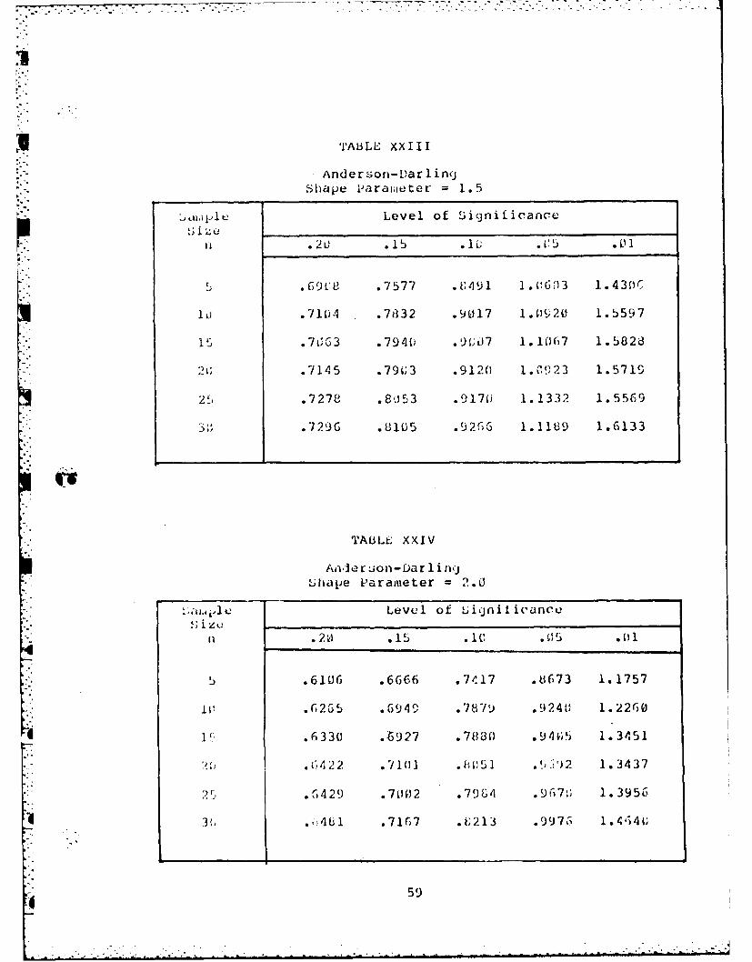
TAiLL XXIII
Anderson-Dar 1 ingShape Paraldeter = 1.5
Wap1I V Level of Signiiicance
r, .2i) .15 .iL .0:5 .0 1
5 .69C8 .7577 .6491 1.(!603 1. 430C,
1 kI .7104 .7d 32 .9017 1. 0120 1.5597
15 .763 .7940 .9(107 1. 1607 1.5828
2k: .7145 .79(;3 .9120 1. C',9 23 1.5715
2 .7278 .8j53 .9170 1.1332 1.5569
3! .7296 .8105 .92 G 1.1189 1.6133
TABLE XXIV
Aav-er:on-Darl inrgShape Parameter = 2.0
1',a, cLevel of Ligniticance.o .15 Ic .1 1, 5.1 1 .05 .0)1
5 .6106 .6666 .7417 .8673 1.1757
10 .6265 .6940 .787w .924;1 1.2260
4 ]! .6330 .6927 .7880 .941;5 1.3451
6, .6422 .710] .8 151 5)2 1.3437
4 .5429 .7002 .7984 .967o 1.3956
3(, .,4 b .7167 .U213 .9976 1. 4,)4 ,
4 59)

TAbiLE XXV
Anderson-DarlingShape Parameter = 2.5
Level of ,'8ignificancei '>;i ze ,__ _ _ _ _ _ _ _ _ _ _ _ __ _ _ _ _ _ _ _ _ _ _ _ _ _
n .20 .15 .10 5 .0l
! .5700 .6261 .6964 .8324 1. 197(,
,1 •.5f",9 I G 5 C,4 .74019 .8740) 1.2080
15 .5915 .6556 .7330, .8693 1.2046
2, 1.9 .6699 .75 4 .9029 1.2276
25 .5991 .65918 .7462 .9023 1.2328
"30) .51311 .6573 .7394 .91J25 1.2614
TABLE XXVI
Anderson-DarlingShape Parameter = 3.11
Level of Significance
.20 .15 .10 .0'J5 .I
5 .5549 .5962 .6730 .7V13 1.0634
Ii .5687 .6276 .7 056 .8415 1.1702
15 .5757 .6376 .7251 a615 1.1651
2() .5749 .636w .716" .8755 1.1499
. 25 .5708 6364 .7225 .C80 3 1.1714
K 3,) .5352 .6490 .7355 .8 28 1. 2601
K- .
"46

TABLE XXVII
Anderson-Darl in
Shae parawc-ter = 3.5
acl , Level of Significance
n .21, .15 .1c .05 .01
5 .5472 .5967 .6588 .7748 1.0173
il .5522 .6024 .6730 .8 u72 1.1318
15 .5577 .6209 .6942 .8081 1.115V
2o .5686 .6259 .7061 .8432 1.1503
25 .5603 .6190 .6960 .8418 1.159{1
3; .563 .6130 .6973 .8298 1.1755
TABLE XXVIII
iAnderson-Darl ing-hape Paraw eter = 4.11
, :a .1p Level of Significance
n .20 .15 .1) .05 .01
.5293 . .,464 .7535 .9715
* i! .5475 .5996 .672 .8 1.1020
15 .5435 .6 ()6 .681( .8154 1.1036
2 G .5565 .6060 .3915 .82(44 1. 1021
25 .5557 .6124 .6998 .8425 1.2094
43; .5577 .6193 .P)7 o .8239 1.161 Ii.

APPENhDIX C
'Pal-les of the Craer-vof l is3es Critical
V~le~;for the Gammna Distriboution
66

.- - - 4 k L : - ' L ¢ /-_.
, :- --,- *: -i -: - . -. : - , - - -- -- -
TAbLE XXIX
Cramer-von Mises
Shape Parameter = .5
i r;at1e Level of S;ijnificance, ;ize
n .20 .15 .111 .05 .01
5 .1217 .1363 .1576 .1928 .3200
0 .1327 .1530 .1795 .2259 .3569
15 .1379 .1596 .1863 .2340 .366o
20 .1425 .1625 .1918 .2526 .3743
25 .1453 .1654 .1951 .2514 .3769
3o .1440 .1649 .1986 .256E, .4170
TABLE XXX
Cramer-von MisesShape Parameter = 1.0
Sarijple Level of Sigjnificance8 ize
.20 .15 .10 .05 .01
5 .1397 .1561 .1809 .2314 .3571
.1341 .1511 .1775 .2210 .3573
15 .1310 .1490 .1738 .2112 .332 .'
90, .1316 .1484 .1748 .2220 .3327
25 .1299 .1487 .1742 .2250 .3239
31 .1319 .1501 .1757 .2228 .3415
63

TABLE XXXI
Cramer-von kIisesSha1 e Parameter = 1.5
-°titpltl Level of S;ignificance-i ze,V, 2 .15 .10 .05 .i
) .1092 .1210 .1390 .1741 .2363
1(, .1132 .1268 .1471 .1015 .2671
15 .1133 .1287 .1541 .1846 .2740
20 .1199 .1353 .1551 .1917 .29,2
S.1157 .1307 .1503 .1847 .2791
3.) .1171 .1324 .152 .1870 .2872
riBLE XXXII
Cramer-von misesShape Parameter = 2.0
p a e Level of SignificanceS i ze
n .20 .15 .10 .115 .01
5 .10I7 .1118 .1261 .1A81 .2096
.1 i45 .1160 .1336 .1620 .222F3
15 .104C .1154 .1325 .1627 .2409
2C; .1055 .1169 .1355 . I([86 .2404
25 .1051 .1174 .135r .1695 .2481
,..36) .1077 .1220 .1415 •1739 .25901
64

'l'TAtOl" XXAIII
Cramler-von i A1'L s.(;hiat.e Iyar ajeter = 2.5
i ;al, pLe I.evel of ,ijnificance
.2o .15 .1 .15 .01
5 .095,3 . D153 .1187 .1432 .19 (;j
. . l1j3 .1263 1522 .2194
109013 .1100 .1261 .1531 .2217
2 . 1) 91 .1097 .1256 .1531 .2207
-.21979 •1099 .1277 .1547 .22.19
-7 3i .1091 .1255 .1543 .2237
TABLIE XXXIV
Cramer-von Njises;hape Parameter = 3.r,
,e Level of Significance
n .20 .15 .i .05 .01
9 .927 •1011 .1145 •1367 .898
o 4 •09 .1042 .12.0 .1441 .2052
15 .0l954 .1075 .1234 .1501 .2085
S'942 .1057 .1214 .i514 .2,1(1
25 .(,()35 .1050 .12-24 1524 .2137
3.9,957 1'b1 .1247 .1521 22 6
I| 65

TABLE XXXV
Cramer-von Mises,hape Parameter = 3.b
;a!,,iple Level of ,;inificance
n .21 .15 .10 0 5 0 1
5 .,919 .1009 .1127 .1341 .1827
10 .0914 .1006 .1149 .1396 .2007
15 .0925 .1032 .1172 .1418 .2002
21 .0939 .Iu51 .1203 .1473 .2112
25 .0920 ."1134 .1139 .1447 •2115
3; .926 .1024 .117(; .1416 .2056
TAHLL XXXVI
Cramer-von Nises
Shape Parameter = 4.0
::J:;aplu Level of Significance
•21 .15 •10 .0 5 il1
.0839 .0968 .11 V9 .1295 .1763
12 .8906 . 102 .1150 .1391. .1974
15 .915 .1F12 •1152 •1396 .1967
2'. .0908 . 115 .1151 .1424 .1959
2, .916 1021 .1182 .1433 .2110
0- - 3. .092 .10 19 .1178 .1431 .205c
r..,

AIP
~.L otthe Korl ~o-i.irnovo ofroCritical Values versus the

LEVEL=.Ol N=5
Lli
co
ci
0
Th. co 1.00 2.00 3.00 4.00SHFIPE PARAMET[ER
FIG; 7. iie. vs K- Critical Valucs, Level =.'.I1, n S
46
SHAPE VS CRITICAL VALUES
:. OnririA
c'J_ LEVEL=.O1 N:-IO
D
0
)
w
(r)
-J -
-C)
v-
0
0.00 1.00 2.00 3.00 4.00SHAPE PARAMETER
"I'; b. ",,iU vi r-8 Critical Values, Lev l .t , n = 01

T9- I
5 SHAPE VS CRITICAL VALUES
GAMMA
r- LEVEL=.Ol N=15
CD• CO.
(.f) c-
1J-o
co:
r-J
.. -J- cici
H-
coN
)(04u -
0. 1.00 2.00 3.00 4.00SHAPE PRRAME 4ER
" , v; V-: Critical Vaue, Level , n
7 1)4 7

SHAPE VS CRITICRL VALUES
GAMMA
LEVEL=.0I W420
C)
LuI
CE
C:
I-
NN
0
'b. oo 1.00 2.00 3.0 40SHPPE PRRRMETER
1;jI. : ii vsi K-S Critical Values, Level =.021, n 21
71

SHAPE VS CRITICAL VALUES
GAMMA
LEVEL=. 0 N=25eli
-4
cli
U)
ci:
Li
CJ
C) 0
00 1.00 2.00 3.00 4 .00SHRPF PRMETER
L i, 11. I..;,e vs K-S Critical Values, Level =.ln =25
U 72'

SHAPE VS CRITICAL VALUES
GAMMA
LEVEL=.O1 N=30
C-.
'0)F-4.
)
WC.)".001.02.03.04 0
-JP PRMEE
I Ao si rtclvle , QC 0 ,n 3
U7

SHAPE VS CRITICAL VALUES
GRMMFI
LEVEL.05 N=S
1)
__j
CC
I-
CV)
Th. oo 1.00 2.00 3.00 4.00SHRPE FRRRMETER
* LI~ 13 . halpe V-. K-S Critical Vj 1uU.S, LoVi 1 .05, n=5
74

SHAPE VS CRITICAL VAILUES
Cn
* LEVEL-.as N=10Co
0)C\1
*0)
C)
Luo)
-J
C-4
0)
b.oo 1.00 2.00 3.00 4.00SHAPE PARAMETER
11,, 14. chj': vs L.-S Critical Values, L~evel =.5,n =1
75

- ~ ~ 1 77 X .~.
SHAPE VS CRITICAL VPLUES
0:)
LEVEL=.OS N=15
CDr-
C)
C'
CELei
p..
03
ctO 1oI. 00 2.00 3.00 4.00
SHRPE PRRRMETER
FIGj lt. Ai1ai1 o vs K-S Critical Values., Level = ,n =l
76

SHAPE VS CRITICAL VALUES
GAMlMA
00
*LEVEL=.05 N=20
0
C)
UI)
J
cC
S.-
U
030
C3
0
c'*b 00 1.00 2.00 3.00 4.00SHRPE PRAMETER
~IUU-. 'haout. v.. IV-S Critical values, Loe1 .05, n 20
77

SHARPE VS CRI.TICA~L VALUES
LEVEL=.05 N=25
04
N
CD
LI)
-J.
-J OCc
(D
'0.00 1.00 2'.003 00 40
SHPPE PRRRtIETER
LIG 17. ;tji.EA juV! K-S Critic-,Il Values, Level =.015, n=25
78

SHAPE VS CRITICAL VARLUES
GAMMA
-4
LEVELz.O5 N=30C14
0
~C%j
-j
Cc)
OD
(D
0.00 1.00 2.00 3.00 4.00SHRPE PRRRMETER
:,1( l6b. t vs i,-,s critiCa1 Values, Level =.0~5, n 3
79

SHAPE VS CRITICAL VALUES
.-. G A M M A
LEVEL=. 10 N=5
U)LLJ C)
;-:)
:Li
Co
C)
-" •oo 1.00 2.00 3.00 4.00SHRPE PRRRMETER
ti( l '. W , v' ;-' Critical Values, Level .18, n =
...
_ .S , . . . , . . " . . ' . _ _ - . , . ; . .. . . ...

SHAPE VS CRITICAL VALUES
LEVEL=.1O N=10
C0
-j.cCJ
CL
CD
CJ
Cet 00 1.00 2.00 3.00 4.00
SHAPE PRRRMETER4
[I GJ v: 1..-Sh Cr it ical Values, LeVe 1 1~ n
81j

0-0124 941 A MODIFIED KOLROGOROY-SMIRNOY ANDERSON-DARLINO AND 2/2CRANER-YON NISES TEST F.. CU) AIR FORCE INST OF TECHWRIGHT-PATTERSON AF8 OH SCHOOL OF ENGI.. P J7 VIVIANO
UNCLASSIFIED DEC 82 AFIT/OR/NR/82D-4 F/G ±2/i N
lomEohmohmohismhhhhhhhhhhhEhhhhhhhhhhhhE

v.A .
L~L6-12.
.. k

SHAPE VS CRITICAL VALUES
LEVEL=. 10 N=15
U)LLJIcJ
CE
-Jw
Coi
0b 0 1.00 2.00 3.00 4.00SHRFE PRRRMETE<
Vc 21. fiapu vs K-5 Critical Values, Leveil =.10l, n =15
82

SHAPE VS CRITICRL VALUES
GA MM A
cliCr)
YAC%j
004
:)
Dco
-. o .020 .040SHPEPRMTE
-J sK5CitclvleLee 1,n 2
L83

SHAPE VS CRITICAL VALUES
GAMMA
0*LEVEL=. 10 N=25
0
N1
N
-- 4
Co
-oo 1.00 2.00 3.00 4.00SHRPE- PlRfM E T E R
* i.23. 'Iia,,, vs U-F Critical ValueS, Level .1(!, n 25
* 84

SHAPE VS CRITICAL VALUES
GAMMA
LEVEL=.]0 N=30
.- °
U)
_..
-
0)
13.00 1.00 2.00 3.00 4.00SHRPE PRAMETER
FI(G 2 4. 'A4Lc vs I-'Cri tical VatlUCS, Lovo1 -lilt ~ 301
85
.". ..- - - - - - -

.'iA*s' -- - . - -- - ..-7.
SHAPE VS CRITICAL VAlLUES
GRMMR
a)
LEVEL=. 16 N=5
cf)
C,
Li0)
D
10 0

SHAPE VS CRITICAL VALUES
GAMM iA
OCxCo
LEVEL=.15 N=10
COJ
-S-
o-J
aC
0I
'b o 10 .0 .0- 40SHPEPicRMEE
FI (.!U p - riia aus ee
'-47
SHAPE VS CRITICAL VRLUES
GAMMllA
LEVEL=.IS N=15
Cr)
LIJ
CE)
af
~)
oh~o I . 00 2.00 3'.00 4.00SHAPE PRAMETER
F iIG 27. '.-Aiape Vs K-IS Critical values, Level =.15, n =15
El8

SHAPE VS CRITICAL VALUES
GAMA(0
LEVEL=.15 Nz2OC%1
C"-
ID
Li)
:Dca)
uat:
00 1.00 2.00 3.00 4.00SHRPE PHRFMETER
2L U v 1:- Critical VIducL;, Level =.15, 11 20
89

SHRPE VS, CRITICRL VALUES
LEVEL=.15 N=26
U-4
LU
-j
'01.01.0203.04 0
SHPEPAAMTE
w 9 tkCevsi- rtca aus evl .1,n 2
c,90

SHAPE VS CRITICAL VALUES
LEVEL=. 15 N=30
C0
NA
'-4
CD
U)
tL 0
C)
-b0 10 20 3.0040SHPUPRMEE
F1G 10 Salev -sciiclvlus evl .5,n 3

SHAPE VS CRITICAL VALUES
GAMMA
S LEVEL=.2O N=5
CfD
3 C)
W)
cCr
c-) 0:Cf)
CJ
0 0oo 1.0 2.00O 3 .00 4.0 0SH-RPE PRRRMETER
h~IL 31. 1J1,ie vs K-S Critical w~ilues., tcvol =.2(;, 5
92

SHAPE VS CRITICAL VALUES
C - LFVF[=.?l N=10
D
X
C
-4
U
L)
b.00 1 .00 2 .00 3 .00 4.00
~I. SHAPE PRRMETER
FIGi 32. v6 ih-s critical Values, Level =.20~, n= I
9 3

SHAPE VS CRITICAL VALUES
'2 GAMMA
LEVEL=.20 N=16
'CD
:)
ci
-j.
OD
Th.oo 1.00 2.00 3.00 4'.00SHRPE PRRPMETER
IG33. :-,ni Aju vs it-s critical Values, Level =.2o~, n =15.
94

SHAPE VS CRITICRL VAILUES
LEVEL=.20 N=20
'-4
Ld0i
-
-4
Luc
-J
L) .01.0 0 3.040SHP PRMEE
16 3 .- v; c iia a UQ ,Iee 2 ,n 2
-95

_ - . .... 7T77 77~7T
SHAPE VS CRITICAL VRLUES
GAMMA
*0
D
=)to
(D
U,
0
-b. oo 1.00 2.00 3.00 4.00SHAP'E PAIRAMETER
* i HU 3r.~ip v:-. K-S Critical Vu~ ee ~
9; A

SHAPE VS CRITICAL VALUES
GAMMA
LO,
LEVEL=.2O N=30
u -)
D
'-o
m)
-b o10 .0 .040SHPjPRMEE
vs-JCiialVius ovl .1,n 3
cJ97

APPENDIX L~
I..aijis of the AridersoiDaln
Critical Values Verse.s the
Cainna Shape iParaiaer.;

SHAPE VS CRITICAL VALUES
GAMMA
C0Co
LEVEL=.D1 N=5u')
CI)
uJ
CCC:)>0j
I-"Cb
Wkw
Co
Co
'0.00 1 .00 2.00 3.00 4.00SHRIDE PRRRMETER
42kIG.1 7. ;hli v.; A2 Critical ValUes, LeVel =.(!I, n =5
4 99

SHAPE VS CRITICAL VALUES
GA MMRi
C)
0)
-4c
LU
CD
CD
4-
FIG38.~Iaf' v~h 2 Critical values;, Level = ~,n lo1(
1oci

No-.
SHAPE VS CRITICAL VALUES
GAMMA
cJ
LEVEL'. O N=15
C)
0
U
>0
C-- to
0
| '-4°
,U).
0
--
b.0oo 1.00 2.00 3.00 4.00SHAPE PRRHMETER
Ll
'I C; 3'. -v; CW Critical Valut:s, LaveI .t'I, n = n ')
101

SHAPE VS CRITICAL VRLUES
:1 : GAMMA
LEVEL=.Oi N"20
C,I °JCC
-
)
OD
c. . 0 1.0 200 300 40
LJ2
0 2
.- .O0 1.0O0 2.0O0 3.0O0 4.O0
:% SHRPE PRRMIIETER
... ' " LIG 4.;. IhL , vs A2 (ritical Valaes, Level = .(1I, n = 20

i. .. ' . .- ,, . .. ' -. ,' ." . -. - " . ' ",-- ..' .' - - '- - . . ., . ". . . -- . . -'_ -. _ • " " . " - -' .' .- " " -
SHAPE VS CRITICAL VALUES
GAMMA
0-4
LEVEL=.O1 N=25
0,a,
0iL °-J
CI
0
04
0q I II
boo 1.00 2.00 3.00 4.00
SHRPE PRRRMETER
I,; 41. 2ha, vs r Critical Values, l.evel = .ol, n =
103
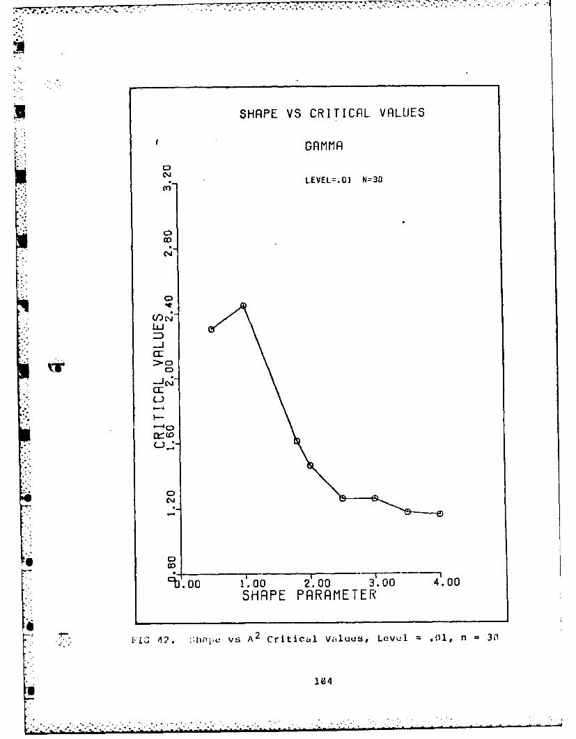
U SHAPE VS CRITICAIL VALUES
LEVEL.0I N=30
C3)
LUJ
c-a
C0
cr_
c1 00 1.00 2'.00 3.00 4.00SHRPE PRRRMETER
I'I G £2 . :',hope vS A2 Critical Values, Level o .0, n =311
104

SHAPE VS CRITICAL VALUES
GAMMA
. LEVEL=.05 N=5
C)
0
C
(-j
cc
C)
>0
_.
I-~
-o
0
00O0 1'.O0 2.00 3 . 0 4 . 0
SHRPE PARRMETER
kI(; 43. L-'-we v A Critical Values, Level .05, n 5
10• q 1 5

SHAPE VS CRITICRL VALUES
GAtMMA
LEVEL=.05 N=10
(cm
-LJ
CC>0
to
C)
'b.o .0 .03.040
SHP PRMEE
FI .,aev . rtia0a~s ee (5
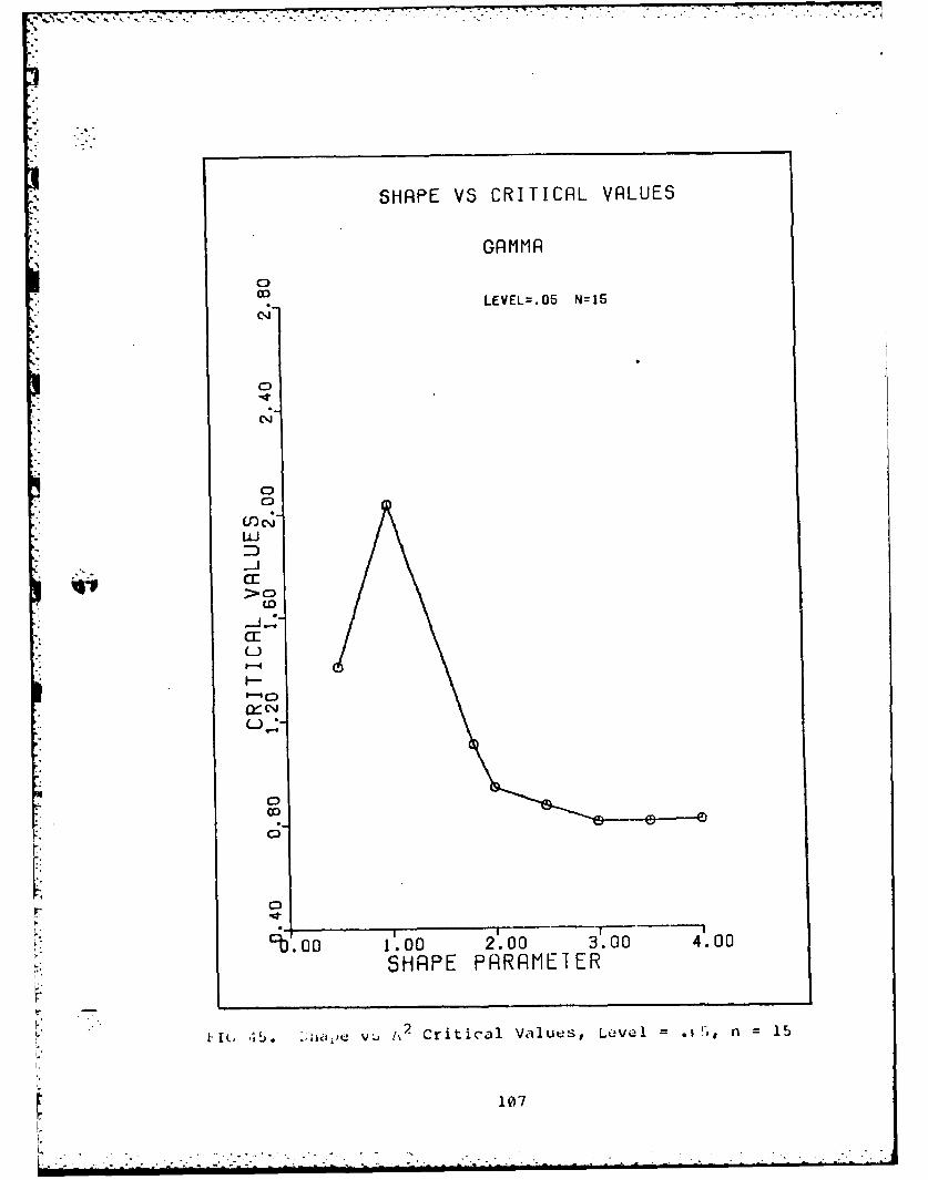
- - - - - - -- - - - - - - - - ..74.
SHAPE VS CRITICAL VALUES
LEVEL=.05 N=15
N
LuJ
-E
>0
":
C)
I-
0
w
cb o 1.00 2.00 3.00 4.00SHRPE PRRRMEIER
iii~~~~ *). .ii v z-critical Value~s, Le VO1 il-, n 15
107

SHAPE VS CRITICAL VALUES
GAMMAip.
LEVEL=.O5 N=20
C%
-4"
0(0LUJ
-:CE>0 CD
b°'1
cc
D
O:c%
'O 0 1.00 2.00 3.00 4.00SHAPE PARAMETER
, "l'l,; 4%. ."l,;[e v~s A2 Critical Vailues , Level = .(.,5, n =2v:
10
%-"
." -.- '-.-, ' ".' - . ''2 ' . " _ -: - , ,. ,. , . - . ' . , . " -0- ' -

U SHAPE VS CRITICAL VALUES
GAMMA
LEVEL=.O5 N=25
C)
U
c-
>0 c
I-
14 0
0
Tho .0 . 2.00 3.00 4.00SHRPE PRRRIIETER
FIG 47. Iat vs A2 Critical Values, Lcvkil =.0~5, n =25
10~9

SHAPE VS CRITICAL VALUES
GAMMA
LEVEL=.05 N=30
C3J
CD
Lli
:D>0
Tw-i-
QCJ
cb 00 1.00 2.00 3 .00 4.00SHRPE PRRRMETER
.7 1 ( 'i. J11JOL' V:,; A2 Critical Val~ue.-;, Level = .;-5, n=
lk)

07
LEVEL=. 10 N=5
0
IC
LJ
CC
C-)
0
0
9j. oo 1.00 2.00 3.00 4.00SHRPE PRRRMETER
VIC' 4'. :h A2Criticali ValuCS, Levul =.(,n 5

SH-RPE VS CRITICAL VRLUES
GAMMA
LEVEL=.10 N=10
cli
0
(D-
-J
CE
CJ
C)
I-
0
Th 00 1.00 2.00 3.00 4.00SHAPE PARAMETER
*L P.i; ::11aijc VS A Critical Values, Level =.1c, n =1
112

SHAPE VS CRITICAL VALUES
p ,q ?" 'GAMMA
LEVEL=. 1O N=15
(DC)
cc>- C
0>0
(3
I-o
,.00 1.00 2.00 3.00 4.00SHRPE PRRRMETER
VI G 111. '~i. VS A2 Critical Values, Level = 1o, n = 15
113

SHAPE VS CRITICAL VALUES
GA MMAP
LEVEL.10 N=20
bLJ
>0 C
0."J
-9
0O,
CD-
Th. oo 1.00 2.00 3.00 4 .00SHAIPE PARAMETER
FIG 52. .,ha,-v vs A2 Critical Values, Level *lt, n =201
114

SHAWPE VS CRITICAL VALUES
LEVEL=. 10 N=25
c:)cm-
-LJ
a:C:00
1-4
C
'.0 1 .00 2.00 3.00 4'.00
SHAPE PARR~METER
[It, 53. :t1 1' VS A: 2 ritical. values, Leve~l .l:n

SHRPE VS CRITICRL VRLUES
K GAMMA
C"D
LEVEL=.10 N=30
- -4
0.2
0
CJ
U
-J
CI:C00
G:
F-
L.." C:-
"0,
CD
I II
00 O0 1.00 2.00 3.00 4.00SHRPE PRRHMETER
H IC 4 11 a ie vs *2 Critical Values, Level = .10, n = 30
r11

SHAPE VS CRITICAL VRLUEIS
GAM MR
* 0
C - LEVEL=.15 N=5
0
-C)D
-:)
Li
U-:
-00o.0 .0 3.0 40SHrE PRcMTE
02
11
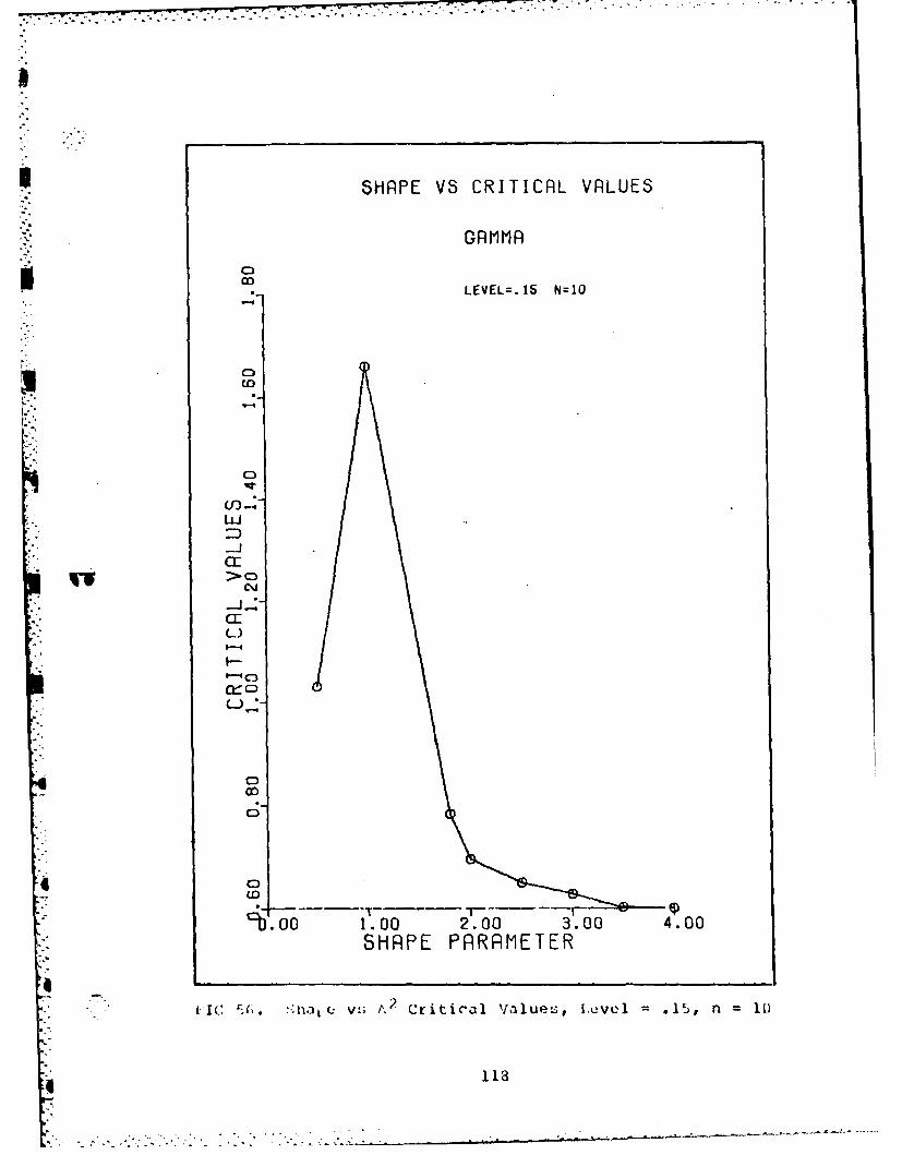
S SHAPE VS CRJTICRL VRLUES
GRMMA
* LEVEL=.15 N=10
C3
::D
CE
LU
~-J2F a I rtclVlus :vl .b

SHAPE VS CRITICAL VALUES
GRMMA
0CO
LEVEL=. 15 N=15
U-
LUJ
CJ
Il-
0
0
OD
Th.oo 1.00 2.00 3.00 4.00SHRPE PARAMETER
5i s7 'tiapc v-, i\ Critical Values, Level1 .15, n~ 15
119

SHAPE VS CRITICAL VALUES
LEVEL=.' IS N=20
0
C~
>0
12
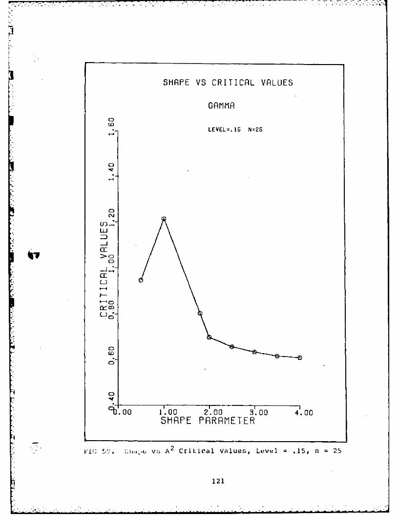
SHAPE VS CRITICAL VALUES
GAM MA
tEDLEVEL=.15 N=25
C.,J
LLJ
-
)
-4
'C)
M
'b. oo 1.00 2.00 3.00 4.00SHRFE PRRRMETER
!IC IL' VS A2 Critical Values, Level .15, n 25
121
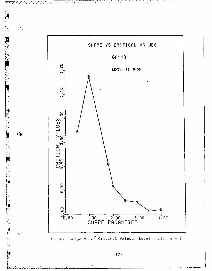
SHAPE VS CRITICAL VALUES
" GAMMA
Q
LEVEL=.15 N=30
:C:
0
U0
(I)
_J
>0
0
.-
I I I
9" O0 1 .00 2.00 3.00 4.00
SHAPE PARAMETER
. I'I.; <i;. "i,,, vs A2 Critical Values, Luvel = .15, n = 3(
122

SHAPE VS CRITICAL VALUES
GAMMA
LEVEL=.20 N=G
0
CJ
LUJ
CE:
-o:C'.
C).
0
CV 00O 1.00 2.00 3.00 4.00F SHAPE PRIRRMETER
i1~1.~v., A~ CritiCal Value:;, Lcvl =.20, n 5
123

SH-APE V3 CRITICAL VALUES
GAMMAC0
LEVEL=.2O N=10
Lu
t-4
c
C)
~~124
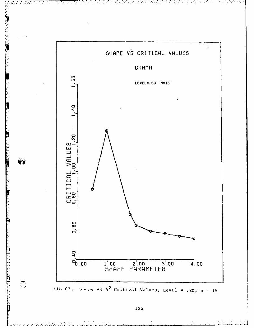
SHAPE VS CRITICAL VALUES
C)
LEVEL=.20 N=15
~0
CJCM-
LUJMJ
CC:>0C
C:
0
Lo
9b. 0 1.00 2.00 3.00 4.00SHAPE PARAMETER
6B (3 Woa*,0 V6~ A- Critical Valucs, Level .20, n =15
125

SHAPE VS CRITICRL VALUES
GAMMA
CDLEVEL=.20 N=20
-4
CJ
-J-:
a:)U;2b
C)
'b o 1.00 2.00 3.00 4.00SHRPE PRRRMEITER
FIjG C4. Sjha; 2 V I; A2 Critical Values, Level .20, n =20
4 126

SAPE VS CRITICAL VRLUES
CR MM R
C0
LEVEL=.20 N=25
-
-
0
CI)'LO
b o10 .0 .040SHP-PRMEE
>0' . ri ia a u sLv l .0
012

SHAPE VS CRITICAL VALUES
GA MM A
* LEVEL:.20 N=30
0
UC-
C)
L)
F-
CD
0
Th. oo 1.00 2.00 3.00 4.00SHRPE PRRPIMEIER
I'lG 6f,( Shwje vs A2 critical Values, Ltovel =.201, n =31
1 23

APPI'''L)Ix k,
Gr~ Li ts o f the Cranter-von t-tise~
Critical Valueii Vor,.,es Ltie
Czmhia shap~e Plaraiiieters
120

,. .- 4 - -.. -.
*SHAPE VS CRITICAL VALUES
GRMMR0
: LEVEL=.Ol N=5r0
C;
C"-
Li
23
-Jccl%
C)J
0
Th. oo 1.00 2.00 3.00 4'.00SH-RFE PRRRMETER
II(7. vi;~C criticalu values, L.ovel .01, n
130
... *

' .c -'.-.'-- -t
- SHAPE VS CRITICAL VRLUES
GARMMA
' LEVEL=.O1 N=1O
C.)
Co~
Li:D
>Co
,JJ
i
CE)
(If C'J
Cbo0 1.00 2.00 3.0 400SHRPE PRRRMEIER
*'u rGE 5. iha,,c vi. h" critical Values, Level =.(')I, n li
131
aa

SHAIPE VS CRITICAL VRLUES
GAMMA
LEVEL=.O1 N=15
C)
N
LUJ
.~j
I-
(J5
U
c-
9.00 1.00 2.00 3.00 4.00SHAPE PRAMETER
i; ~m mz~. ~ 2CriLic'1 Values, Lcvel=.1,n=1
* 132

SHAPE VS CRITICHL VALUES
GA MM A
* LEVEL=.O1 N=20
C7)
C,
-
to
'00 .020 .040
SHPEc:;MTE
cc2j G 7; ,hiov rtia au-),Lv ln 2
I13

SHAPE VS CRITICAL VALUES
GAMM1A
LEVEL=.D1 N=25
0
C)
LLu
-JO
C)
C
C3JC I
'0.00 1.00 2.00 3.00 4.00SHRPE PRRRMETER
K ~~ ~ L v tiG N1 ,d~ CriLiCal Values;, Level = .i1,
134

7 SHAPE VS CRITICAL VALUES
GRMrIR
LEVEL=.OI N=30
0
Q
C;
(no
-J
c:Cr)
cin
I-
I...
D
4 1w
Th 00 1.00 2.00 3.00 4.00SHRPE PRRRMETER
ii72. !jaj;c w;~ Critical Values, Lovel .0ll, n 3
135

SHAPE VS CRITICRL VALUES
GAMMA
C:)- LEVEL=.05 N=6
C)
Q
LU
LiCE
CE
N
1.L2.0 '0O 40
ULJ
0

SHAPE VS CRITICAL VALUES
GAMMA
_ LEVEL=.05 N=1O~0
)oLUI
-
ic;-a:
--
(-5
•I III
-00 1.00 2.00 3.00 4.00SHRPE PRRRMETER
'1 -4. .%'2 Critical VlIues, Level = .05, n IA)
137
- . . --!,---

SH-RPE VS CRIIICRL VRLUES
ORMMR
C~j CEVEL=.05 N=150
CJCLi-i
CE
C-
F-
co
Too 1.00 2.00 3.00 4.00SHAPE PRAMETER
tFic 71,. VL 1 -.2 Critical1 Value s, LCV(el =L.5, n =15
138
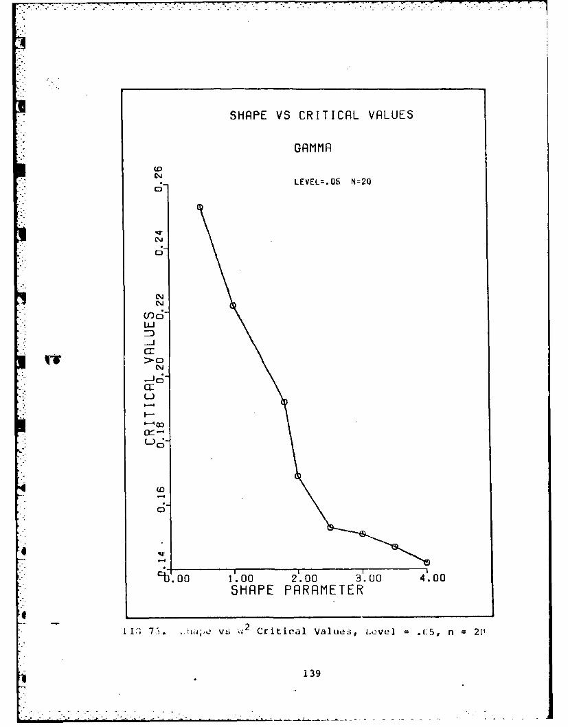
SHAPE VS CRITICAL VALUES
GAMMA
(D
C;- LEVEL=.05 N=20
0
CJ
LuJ
-JccE:
>0
.13

SHAPE VS CRITICAL VALUES
*LEVEL=.05 N=25
N
C
o
i
-Jc
Lj )
14

SHAPE VS CRITICAL VALUES
GAMMA-
to
0* LEVEL=.f35 N=30
0
)
L)
CJ
co>0
'o N10 .0 .040SHP PRcEE
C.J2
FI 7( hvCs.IDrtclVle , ee 0,n 3
-14

SHAPE VS CRITICRL VALUES
GA MM A
CMj* LEVEL.1O N=5
C).
-9
-LJ
cc
I-
C'.'
00 1.00 2.00 3.00 4.00SHRPE PRRRMEIER
lAG ~ ~ V 7 U 2~ ~ Critical Values, Level .10, n 5
142

SHAPE VS CRITICAL VALUES
LEVEL=.1O N=10
C)
LuJ
CE
0
c4
cb 0 1.00 2.00 3.00 4.00SHRPE PRRRMETER
12I IG '8 .1p v ; W Critical values, Level .ln=
143

SHAPE VS CRITICAL VALUES
GAMMR
0CJL .1 N 1
C
-i
Li
>-(
F-
$- It
9xoo0 1.00 2.00 3 .00 4.00* SHRFE PARRMETER
Flu !I. Shatu v.. . Critical Values, Levul h 1t, n 15
144

SHAPE VS CRITICAL VALUES
GAMMA
C* LEVEL=.1O N=20
0
0
CE
LU
-
C:
(3
'0.00 1.00 2.00 3.00 4.00SHRPE PRRRMETER
F IG 1!2 ;iicm ~,,~critical Values, Level Iol~, n =20
145

SHAPE VS CRITICAL VALUES
K GAMMA
N LEVEL.IO N=25
CJ
M0
-4c
C(f)UC3
0
C 1.0 0 2.03.0 0SHP PRMEE
(J21:.I-p s Ciia VleLvl 1" n 2

SHAPE VS CRITICAL VALUES
GAMMA
C i
0
u-I
c-
>LO
-E
0
9oJ.00 1 .00 2 .00 3 .00 4.00SHRPE PRRRMEITER
4
iv;.- ~. ~ V. Critical ValueS, LtuVel =.(,n 31
74

SHRPE VS CRITICRL VPLUES
GRMMR
0,U,
LEVEL=. 15 N=5
0r)
U)
LLCD
)C)
01

SHAPE VS CRITICRL VALUES
GR MM A
0
* LEVEL=.15 N=10
CD
0
)K
U)Lij C
0
C)
oh o 1.00 2.00 3.00 4.00* SHRPE PRRRMETER
i~; r. ~ vs Critical values, Level =.15, n=
g 149

SHAPE VS CRITICAL VALUES
GAMMA-
! Co_ LEVEL =.15 N=15
Ln
U)
-is
CE,:. --
U
0
0
& t
-b. oo 1.00 2.00 3.00 4.00SHRPE PRRAMETER
i IG ,f7. l vs tN2 Critical Values, Level .15, n = 15
151)

U.' SHAPE VS CRITICRL VRLUES
GAIMMR
LEVEL:.15 N=20
c15LLU
CE
-j
cr
)
1151

SHAPE VS CRITICAL VALUES
GAMMA
cm LEVEL=.15 N=25
C-
C-
LLJ
CC
CE
-o
)
00
C1 1.00 2 .00 3.00 4.00SHRPE PRRRMETER
ii. ~.v. ~ V ** 2Critical Val1ues, Lovel =.15, n =25
152

SHAPE VS CRITICAL VALUES
GAMMAi °i
I CJ LEVEL=.IS N=30
Lo
CE
CE
C)
C)
1.00 2.00 3.00 4.00SHAPE PARAMETER
,
FIG V .wp V 2 Critical Values, Level = .15, n =3
153

SHAPE VS CRITICAL VALUES
GAMMA
C0
LEVEL=.2O N=G
0
'0
Dc'.C,
CE
0
'b o 1.00 2.00 3.00 4 .00SHRPE PRRRMETER
F'1G 9, 1. S1hape vi; N2 Critical Vailues, Level =.202, n =5
* 154

SHAPE VS CRITICAL VALUES
LEVEL=.20 N=10
OD
C),
-4
(I)
LU
cb.0 .0 0 .040
-J. PRMEE
I' . .cr t c l V lu s e e .1, n 1
-15

SHAPE VS CRITICRL VRLUES
GAMMA
0)
LEVEL=.2O N=15
CO,
LLJ~~
n-4
CE:
-
C-.j
00. 0 0 1.00 2.00 3 .00 4.00SHRPE PRRRMETER
1, IG1 93. iiape v.i critical ValuteS, Level .20, n =15
156
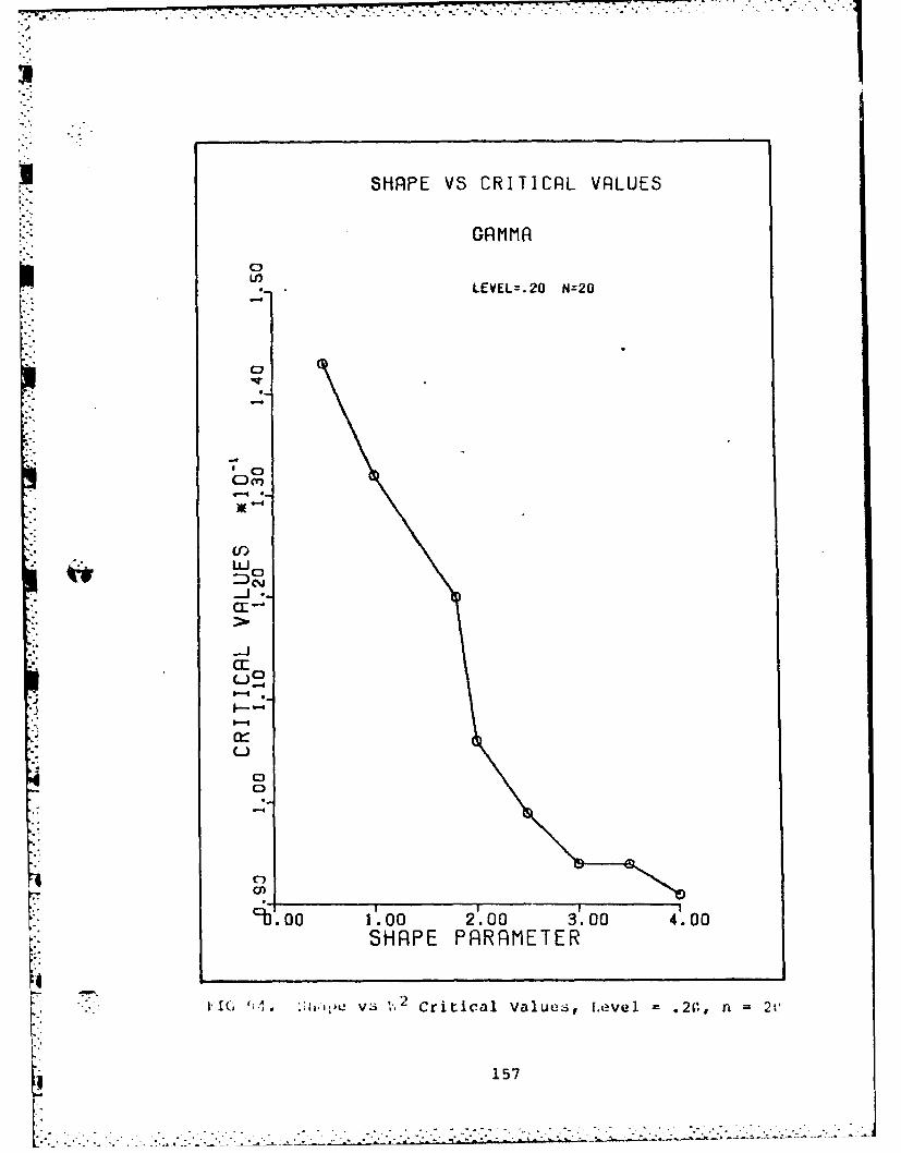
. SHAPE VS CRITICRL VRLUES
GAMMA
C,•) _LEVEL=.20 N=20
C-
.4-
4')
b.4
•~- . -.
crp-.,,-
C)
-4
C,
'"1 00 1.00 2.00 3.00 4.00SHRPE PHRRMETER
FIG ".. L-, vs '.2 Critical Values, Level = .201, n = 2'
157
. . ~ ~ ~ ~ Li . ..--.. ..-- . .- / .. :

SHAPE VS CRITICRL VRLUES
ORMMA
Li,p•-4 LEVEL=.20 N=25
w--..
C31
LU)
°. 4.
cr
-Ja:
4 C)
c -j5-' 0 I I
.00 10 2.00 3.00 4.00SHRPE PRRRMETER
I'
- . iIC V. , ,.,, Vi 2 Critical Vi.luei, Levul = .20, li 25
158

SHRPE VS CRITICAL VALUES
GAMMA
LEVEL=.20 N=30
U4
4
'Oo..
cr
)
',-J.
-D
-159
*g 0
cb~oo 1.oo 2.00 3.00 4'.00
SHRF'E P RIJE TER
:'-" ~I, ,)* .tla~ vuj t.* Critical Values, Level' .?. , n =3
159

'N D I X G

~PROGRAM AD
C
C *THIS PROGRAM GENERATES rHE 4OOIFIED A-D STATISTICSC o5000 RIPS *
C THE TABLES GENERATED ARE VALID FOR THE GAMMA DISTRIBUTION a
C ft = SAMPLE SIZE : 5%(5)930C IsSSz 0 IF SCALE PAKAMETER (THETA) IS KNOWN aC *SS1 = 1 IF THETA IS TO HE ESTIqATEDOC oSS2 = 0 IF SHAPE PARAMETER (K) IS KNOWNC *SS2 = 1 IF K IS TO UE ESTIMATED aC eSS3 = 0 IF LOCATION (C) IS KNOWNC *SS3 I IF C IS TO BE ESTINATEDC eCl = INITIAL ESTIMATE OF C (OR KNOWN VALUE) aC eTl z INITIAL ESTIMATE OF THETA (OR KNOwN VALUE)C *A= INITIAL ESTIMATE OF ALPHA (OR KNOWN VALUE)
COMNON/VALUE/P(100)COMMON/RAY/T(100)COMMON/MANA/NSSI*SS2.SS3,NwCer tI o1NRDOUbLE PRECISION OSEEDoToCloTLeAIDIMENSION FX(6bO)AA(50001XK(002)oY¥T(5002) 6(50)INTEGER REP9PPOSEED=150 00.000MR-O
NONE :0NZERO=OREPzbO02NDS=REP-2NUMZREP-2
CCC &CALCULATES 5000 PLOTTING POSITIDNL. ON INTERVAL (0911 At (I-053/NC sTtwESE ARE USED FOR INTERPOLATIONS ON PERCENTILESC
VYI REP):I.00 405 L=2oREP-l
VTY(L):( (L-1l-.51/NOS
405 CONTINUEC 6END OF PLOTTING POSITIONS R3UTINE
READ AO#,SSS2. SS .53*CT rl*AtPRINTavSSl#SS2pSS39ClvTloA1PRINT*PRINTPh~INTOPR.NTt(2XA.F5 .1et'SHAPEz:9AlPkINT9(2X9A)9 so ----------- 8PRINT*
C *SAMPLE SIZE ASSIGNED HERE00 100 PP:15025N:PPM:N
C *LOOP FOR MONTE CARLO SIMULATION STARTS HERE00 99 KK:=15000CALL GGAMR(OSEEOAlNeGP)
161

*~0 119 coKri 9N
CALL VSRTA(PNl00 3 11=19N
3 CONTINUECALL GAMMA(tCSJ rSJASJ)
C *CALCULATES LST[MATEO FIX) FOR~ EACH SAMPLE POINT00 335 LzlohM=IPIL)-CSJI/TSJXI=ASJCALL MDGANME9I9PRO8gIER)FXtL I=PROBIF(FX(L).EQ.Go)T1IENFX IL 5-F N LP*. . 01NZERU=#ZERO.1END IFIFIFX(L).EQ.L.)THENFX4L 3:FX(LI-.OO01NONdE NONE.1END if
333 CONTINUEMA 0:0.XN=N00 500 1=19N11:1MAD=WAD.12.eXI-l.).(LOGIFK(I )3*L06(l.-FX(N*1-I5)I
500 CONTINUEMAD=I-MAD/xkd-XkAAtKK):UAO
99 CONTINUECALL VSRTAIAA,5000100 400 L:1,REP-2
400 CONTINUECALL ENDPTIXoVVREPgNUN)
CC *PAINTS, PERCENTILESC
PRINTl(2XA,12)lv9FOR N = 0PPPRINT9(2X9A)990 ----------PR INTs00 410 J=8099595DO 420 11=1.REPI=REP*1- IIIFEVYtl ) LT. (J/100.O3 ITHEN
ZZ=-SLOPE*XX(I I.VVII)PRlNTt(2X9A, 12jA#F9oW9'
19THE*,JoIT PERtCENTILE IS',24(J/100. )-ZZ)/iSLOPEPRINT*GO TO 410ENO If
420 CONTINUE410 CONTINUE
10G2

00 430 AK=19REPK=REPOI-AKIFITTIC) .LT. .99)TIEN
60 TO 999END IF
430 CONT INUE
Liz- SLOP a EXt K) ( K)PR INT* (2 XA, f9.4)
IOTHE 99TH PERCENTILE IS2,24.99-ZZI/SLOPEPRtIN T*PRINraPR INT&PRINT*
100 CONTINUEPR INTO (2X9F9o* 94v~44XF.) qCSJqTSqJvASJElio
CCCC 0SUBROUTINE TO EVALUATE ENDPOImrsCCC
SUBROUTINE ENDPT(XXYYREPvNUHIINTEGER REPDIMENSION XX4REP),TY(REP)SLOPE=(VY(2)-VY(3) )/CKX(2)-XXIS)a3zlY(2)-SLOPE*XX(2)Viz-el SLOPEIF(VI.LT*Q*)THEN
VI:O.END If
SLOPE:CYIINUMI-VV(NUM*ib)I(XX(NUN)-XE(WtUN,1))B1i:VT(NUH)-SLOPEBeXINUM)V2=(I.-01)/SLOPEXX4REP)=V2RETURN
163

PROGRAM PIOGGI 74/i, OPT"- FTN 5*1*52g
PROGRAM 110G61
C THIS PROGRAM GE1dCRATES A POW7q STUDY BETWErk THE FOLLOdINGv'C KS.CRAMII_ VON-MIStS, A4O7_RS0N-4ALINGv AND CI-SQUARE STAfC 5000 REP"C THIS POWER STUDY IS VALID FOR rTH GAMMA DISTRIBUTIONC N =SAMPLE SIZE z25 TC SSE:O IF SCALE PARAMETER TH-T IS KNOWNC SS1:1 IF THETA IS TO BE ESTIMATED 4C SS2=O IF SHAPE (9) IS KNOUVdC SS2=1 IF IKI I-S TO BE ESTIMATE)C SS3=0 IF LOCATION (C) IS KNOWNdC -SS3zl IF C IS TO BE ESTIMATEDC CI=INIFIAL ESTIMATE OF C (OR KVOMN V4LUE)'C ' TI:INITIAL ESTIMATE OF THETA ()A K14OWN VALUE)C AIzINITIAL ESTIMATE OF 9 (OR KIDUN VALUEDC s* 1U *t 4. k~ a 0. 6 ,~ a &
COMMON/VALUE /P(100 ICDMHON/RATIT(1001COMMON/MANA/)..SSI.SS2,SS3,MC1,TlA1.mqDIMENSIONe FX(601.@FIX (60),
2AAWdCVM(SOOOI .AAhA(50001,AAKS(j000)DOUBLE PRECISIOV OSEED*T#:1,rIAIINTEGER PPOSEED:25000. ODDHR=0RWCVM:O0.RWKS=O.
NONE :0710 CONTINUE.
READ eSSI*SS529SS3*CI ,TlAIPRINT' .SSESS2.SS3*C1,TI*AlPRINTPRIN~tkPRINTPRINT*42XvAvF5.I1 ' .SHAPE~' ,I1PRINiT9(2X9Al* to--------------------PRINT-
kPPI
M=NdDO 99 KK=195OOOCALL 6GNLG(OSEED.N*D.,1.,3#DO 719 IKZ1,NP(IKI=1. P4LKI*10.
4 119 CONTINU.CALL VSRTA(PoNlD0 3 XJ=ION7(IiI:P( IjI
3 CONT INUECALL GAMMA4CSJTSJvASJi)DO AS Lz1,N
U:(T(Ll-CSJl/TSJ

PROGRAM P10561 74/74 OPrag FTM 5.1*52B
XX:ASJCALL MOGAM(U.XX*PROBIbIR)FX(LI=PROBFIX( Li :F I(LbIF (FIXtLO.iQ.O. ITHENFIX(L=F IXtL)*.oO01
END IFIF(FIX(L I .o.. to I THENFIX(LlzFIX(L)-.0001NONE=NtON.* 1
TOP: 0.BOTz0.DO 500 I119
RL =IF(RL/XN-FIX(Jb *GT. TOP$ TOPzRLIKN-FIX(I)
UCVM=UCWH.(FX(Il-(2* Xl-?.olf(2* XNIS 2
500 CONTINUE
IFSBOT *GT. OIFlOIF=BOTIKS=DIF
AAKS (KICIOFIF(WKS >* *27)!lRKSRiISe1.MCWM=WCVP41. i(12.,XNIAAMCVM(KK i=WCVMIF(MCvM .GT. *1391)RWCVNRICVIO1*WAD=4-UA D/XNI-XNAAWAO(KK I:UAOIFIMAD *GT*.803IP RWiAD:RWADe1
99 CONTINUE'CALL VSRTA(AAKS,50000CALL VSRTA(AAWCVM950001CALL VSRIAAuA3#5O0OiPRINr.PRINT- 9*NZEROZ ',NZEROPRINT*#INON-= *vNONEPRI[NTPRINT. ,'SANPLE SIZE z 09PPPRINTPRINTPRINTb is*TOTAL RrJECTION 2 FOR I-Sz ',RWKS/5000
* PRINT'PRINT-91TOrAL REJECTION I FOR JCVR= foRWCVM/500APRINTPRIN to 99TOTAL RZrJEC TION I FOR d43= *,RWA3/5004PR INTPRINTPRlkT'(2XF9.4tAXF'i*iAKF9.AI'CSJTSJASJ
*~ ENO

CCC *SUBROUTINE GAMMA CALCULATES MLE PARAMETERSCC
SUBROUTINE GAMMA(CS.,,TSJASJ)COMMON /kAY/T(100)COMMNI/NtA/t4,SS1,)2.SS3,M.C1.TlA,MNiDOUBLE PRECISION TvCTtIErAALPlA9OLT9DLA9 ALOLC.CETHvEftENELNMDOUBLE PRECISIONM EMrkEI D2TOrD2A.OA,02CDCENSGAMGMAGAMT ,BMAIDOUBLE PRECISION GMA12,OEXP.DABSDLOGSLDGD6I ,06[2.SRS1.DGANDOUBLE PRECISION DGANqIELCS~,TSJASJoC1 ,T1,A1,OSEEODIMENSION C(110Q),TWETA(jI00),ALPHA(11Q0)DIMENSION OLT(t0) ,OLA(505 ,AL(501,OLC(5O),CE(50)T4(5O5Ji:20
THETAC 15 T1ALPHAE 1)=AU
9 EN=NEM=M
86 ELhM=0.0EMR=MRMRP=MR .1
al NMNNH.DO 88 I:NMN
as ELNN=ELNN*DLOGCEIDIF'CMR)669899109
109 DO 110 I11"
110 ELhM:ELMM-OLOGCEIS89 DO 63 J191100
IF (J-11 66,112,111III 5j:jj-l
If IJ-JI)6,139,139139 IF (J/J"-.JJ/JH)6,6,111I11 .12zJ-2
J33J-3IFCSSI1 1 15119,118
11R O2T=THETA(JJ5-2.0O.THETA(J2,.T1ErALJ3IOT:THETA(JJ1-rTETAJ2IF 102T)135*119,135
135 NT=DABSCDT/O2T)60 TO 120
119 NT=999999120 IF (SS2)122,1229121121 02A=ALPNA(JJJ-2.D0eALPHA(J2).ALPNALJ3)
DA=ALPtIAC4J)-ALPHA(j.25:F 402A)1369,12291316
136 hAzOABSIOA/02A)GO TO 123
4122 NA:999999123 IF (SS3)12591259124124 D2C=C(JJ1-2.iUO*.2)CJ31
OCzC iJj -C (J2)IF (CLJJ55.D-5T(15)140v~I252
1

SUBROUTINE GAMNA 74114 OPT=i FTN 5.1.520
140 IF (C(JJ)-5eD-5J125vI259l11
137 hCzOABS(OC/02C1GO TO 126
125 ft.Cz,1*j991126 ftS=2*MIN0(tdTvNANCI
IFtNS5fi68,12
138 ENS=NSIF CSSI)12791279128
127 THETA(%§)=THETACJJ)60 TO 129
128 TICA(J)zTHtTA(JJ)*(OT..25D0e(--iS.1.DOQID2TBE4STHETA(J) :DNAXI(THfTAC.J),1.D-4)
125 IF CSS2)1.3091309131130 ALPHACJI:ALPHA(JJfl
GO TO 132131 ALPHA(J) =ALPHA(JJ3.(OA..25DO .(EM4S..O)a02A3.[NS
ALPHA(J) :OMAXl(ALPgjA4JJ,1.O-4I132 If (SS3)1.3,1339134133 C(J)=C(JJ3
6O TO 112134 C(J)zC~jjfl(DC..25D00.ENS.1.D03aO2C)eENS
C(J)=ONAXI £C(J).0*DQ)C(J)=DON1(J)9TC 1 )IF (1.O0-EMR)*C(J)-T(l))112,&6
6 THETA(.fl=:THETA J)~i. IF iSS1113913,7
7 SI:0.0000 8 I=MRPgN
a S1=S1*TCt),-C(JJbIF IN-N.IIR)6697S,74
73 TNETA(J)=S1/4EN&ALPHA(JJf)Jso TO 13
74 6MA=GAM(ALPA(.iJ))KS Z0DO 108 K=1950KKZK-IGNAI:GAMIC(T (m)-C(JJ)bITHETA(J,ALPHA(J~J)SNMA2GAN(T(iP)-C(JJ)/rlEr?.(j.ALPHA(JJIIOLT(K)=-ENALPH1A(JJI/THETA(J).Sl/(THETA(Jle.2).(EN-EN).(T(M)-C(jjb
1 3e.ALPM4A(JJ) o(EXP((C(JJ)-T(Pq) )/jETA(J))I(THETA(J)..(AL0,1A(JJ)*..u20)3.GNA-GH4A1.JEH.ALPHAJJ/THErAJ-EMe*(TrMP-C(JJO)a.AL'tiA.J
A 6EP(CJ-~oR)/HTCJ/(p~~~e(LHAJI10)GA2
Th4dKI=TN( VA(J)If COLI(K))11 .15102
101 KSZKS.-1IF (CSPK)10591039105
102 KS=KS~lZF(KS-KJ 105,104i,1O5
103 ThCTA(J)z.5D0&TNt(K)46 OTO lob
104 THETA(J)=I.50.TeI(K1GO TO lob
105 IF fOLT(K)*DLT(KK)Jl1913v16108 KKK-
60 TO 105
167

SUBROUTINE GAANA 14/14 OPIZ0 FYN 5.1*524
107 TiEA(J)=TH(K).OLT(c).(THIK)-rH(KK )I(OLTCKK)-W.TEK)$IF £DABS(rHErA(J3-Tgl(KII-tD-4)13.13.1a5
106 CONTINUE13 ALPHAJI=ALPhA(JJ)14 If £SS2)44#44v1515 SL=0.DO
DO 16 ImMRPN16 SL:SL*OLOG(TCI)-C(JJbI
KS=ODO 43 K=1950IK KK-1GMA: GARICAL PHA CJI bIF £N-N.D4R)66.30921
21 GNAI=GANIC CTCMb-CIJJb)/TiETAI(J),ALPHACJ))6NA12=GANI C(TCMqP)-CC(JJl)/TI4ErA(J) ,ALP"A(.J35
30 DG=DGANtALPHACJJ)76 IFCN-PN.MR)66,71,v3271 DLACK1:-EN.DLOG(THETA(J)).SL-E4*G.O/G"A
60 TO IS32 DGZ:OGAMII(T(N)-cCJJ))/TIIETA(J),ALPHA(JJ)
0612:DGANI CCII NRP)-C(JJ))/TIETA(J ,ALPHA(J))31 DLACK)=-EN.OLOGCTI1EIACJ)).SL-EN.O6/GNA.CEN-EN).(D-DGIlI/G6NA-GNAII
1.ENR*DLOG(1I4ETACJ) 5.ENR*DG12/6qAI278 ALtKI=ALP1A(Jl
IF CDLAIK))35,944,4039 KS=KS-1
IF IKS*KblO.4lglIO40 KS=KS*140 IF (KS-K)70942*70
41 ALPHA(J)=.5O~obALlK)GO TO 43
42 ALPHACJ)=1.50.AL(KI* 60 TO 43
to IF (OLACK)&DLA(KK)172,44l1it KK:KK-1
60 TO 7072 ALPHA(J)=ALCKI.OLACK).(AL(K)-ALK) I(DLACKKI-OLAIK)I
7. IF IOABS(ALPhACJ)-ALCK)3-1.0-43444,4343 CONTINUE44 C(JI:CCJJfl85 IF CSS31112,L1294545 IF 41*D0-ALPIIA(J))799143vI43143 IF (SS1*SS2)b1,57qI91s IF £N.-N)66.bJv4646 GNA=GAN ALPIIAIJI)63 KS=0
00 56 K=1954KK:K-1SR :0 * D00 69 I:NRPIN
6 9 SftSR.D.0(TfI[-CJI))IF (N-N*NR)66,80981
so DLC(K):C1.DO-ALPhAC(J)O*SR.ENItNiETA(JI60 TO 82
$1. 6NAZ:GAMIC(UCNM)-CCJI)/ThETA(J)@ALPiACJ)GHA12=GAHICfV(MRP)-C(J))/TIETAJ)ALPIACJ)IDLCCK3:C 1.DO-ALPNIA(5) 1SR*CCn-rnq)/THETACJ).(EN-EN3.ItTIN5-C(J))s.(

SUBROUTINE GHMA 14174 OPT=O FYN s.t*3a,
IALPIIA(J)-l.DO EX((TM-CJ)/HTAJ)/(THETA(J)eeALPH4A(J'(I2A-GNAIb)-ECN&aT(MRP)-C(J))ae(AL~bNA(JI-1.00).OEXP(-(T(NAPI-C~j3)/TNq3ETA(J)3IOCrHETA(J5..ALPIA(J)e6qAI23
82 CE(K)=C(J)51 IF IDLC(K)1909112#91
* 90 KS=K,"-IF (KS*K)54,52954
152 IF(C(J)CLoC () -1D)121,6
53 CONTINUE(K*50(()C(60 TO 112
112 IF (DLCKI oLC(X))fT91295
113 O 15 I1
66 IF (DBC(J )-C(1.GI*-4-TIb16 111129
56 IFCONINUE,560 T1O 112
S1ZS1.)Ttl3-(J
L2 IF(NMRA 66139
IF (NA JI*AeO ((T(N)-C(JII/rI4(JAPIA(
16 If tN-N)668 O0,9
108 SZC(I)C)
GAJAALPHA(J )IF (-*)660,60~f
6 IF (DAMS(C(-C(J))1.D-A(J~1,61 .6361 F A=G ~AMI(RI-C(J))TA~HETA.oIALPHACJII
628 I ELDENaS(A*LHAIJ)-PHAJJ))-L.DO(TE)4,)*ALHAJ,630b
IF6 REUNMN)610999 EL=LND E)(DO(H-MI)DO(N
5-NeL"C~DLG~EAJ)EtkDO(1A2
100I (SJ= .i

FUNCTION GAN TIq OS FYN 5*1+524
CDOUBLE PRECISION FUNCTION. GAHM
* DOUBLE PRECISION G#Z#DLOGOEXP*1
I IF (Z-9*001292,32 GzG-DLOG(Z)
GO TO I3 GAM=G(Z-.500)aDLO(Z)-Z..5OO'3, 06(2. 0a3.Il I5926535897 iBOI*1.0OI
6AM0(EXP(GAM)RETURNEND
FUNCTION 064H 74/74 OPTZS FIN 5.1*52i
DOUOLE PRECISION FUNCTION OBA4CI)DOUBLE PRECISION D6.L,1,OLOSBAN
I IF tZ-9*DO)2t2e3
2 0:061.001
so T0 13 06AN:O6.(Z-.5OO)IZ.0L06(z1-I .DO-1*1.D/(I2oDO*l..2I.1.O0/(120.080?*4
I )-3.00/(252.00eZ*'6).1.32/(200.00aa8 -I.00l(132.00.Za. 1012 *691.O0/( 32760.DO.ZO*12)-l.0I(12.0Q.Ze'14)VGAN:OGANO6AH(TIRETURN
FUNCTION OGAMI 740/74 OPT:0YN51*2
DOUBLE PRECISION FUNCTION OBAMI(WZ)DOUBLE PRECISION uV#UZqSUqELLDIMENSION Ut5O)#V(50)
W(1b=W&Z/Z&&2SUzU(11-Vt1JDO 1 1:2950LL:1-1ELL=LLU(C):(..ULLROUELL&(ZELL-t.D 3)I(Z.ELLI
I SU=Z;U* UI L I-V IL IDGAMIZSUAE TUANEND
17 Cl

UFUNeTION GAHI i7/1y oprI0 FYN Sol*S24
DOUBLE PRECISION FUNCTION GANICM.ZIDOUBLE PRECISION U9UgZvSU.ELLDIMENSION Uttla)
SU:U91 5DO 1 L=2950LL:L-1ELL: LLUIL):(-U(LL)/ELLS eU.(Z.ELL-t.03 5I(Z*ELLI
I SU=SU*U(L)GAII :SURtETURNE ND
171

Vi ta
,'hilij. .John Vi vi ano wj~ iborn on 1,~Ve~fl~r1)8i
:; ntLou i -- iiji-our i * lie jrad ua ted f roc, Sa int P'aul lii.jih
Lcu&ioi iii :.ij iland, Illinois in 19C.". ine rect-ived a baclic-
lot'-s dtjree in Applied ivathernatics froi Southern Illinois
uiiiv%.rsit in 1;cvardsville in 1971. I~e attended Officers
r~4i i~n~ ', Cool c.,r1 was coululi iissionL-d ai; a U.1,14 a LIIiccr in
11)77. ii- ,ore ~ a plannlinj anal -:,t for tue Deputy for
~k~C )j.LV~tk'~un;,lieCtronic -Sytem6u 1.,ivisioii# Hac~rSolu 1ir
Forc iw~e. ~ then entered the : chul it LErinering, Air
Ijorce Im~t itiwLe of: Technology in Iune 19(C 1.
I-Lrmianeflt AddIress: 126 Collinsville Ave.
Collin:-ville, Il. 62234
172

FILMED