actuarial mathematics for life …math.kangwon.ac.kr/~junekim/lecturenotes/acutrialmath/...of...
TRANSCRIPT

2
Survival models
2.1 Summary
In this chapter we represent the future lifetime of an individual as a randomvariable, and show how probabilities of death or survival can be calculatedunder this framework. We then define an important quantity known as the forceof mortality, introduce some actuarial notation, and discuss some propertiesof the distribution of future lifetime. We introduce the curtate future lifetimerandom variable. This is a function of the future lifetime random variable whichrepresents the number of complete years of future life. We explain why thisfunction is useful and derive its probability function.
2.2 The future lifetime random variable
In Chapter 1 we saw that many insurance policies provide a benefit on thedeath of the policyholder. When an insurance company issues such a policy, thepolicyholder’s date of death is unknown, so the insurer does not know exactlywhen the death benefit will be payable. In order to estimate the time at whicha death benefit is payable, the insurer needs a model of human mortality, fromwhich probabilities of death at particular ages can be calculated, and this is thetopic of this chapter.
We start with some notation. Let (x) denote a life aged x, where x ≥ 0. Thedeath of (x) can occur at any age greater than x, and we model the future lifetimeof (x) by a continuous random variable which we denote by Tx. This meansthat x + Tx represents the age-at-death random variable for (x).
Let Fx be the distribution function of Tx, so that
Fx(t) = Pr[Tx ≤ t].
Then Fx(t) represents the probability that (x) does not survive beyond agex + t, and we refer to Fx as the lifetime distribution from age x. In many life
17
18 Survival models
insurance problems we are interested in the probability of survival rather thandeath, and so we define Sx as
Sx(t) = 1 − Fx(t) = Pr[Tx > t].
Thus, Sx(t) represents the probability that (x) survives for at least t years, andSx is known as the survival function.
Given our interpretation of the collection of random variables {Tx}x≥0 as thefuture lifetimes of individuals, we need a connection between any pair of them.To see this, consider T0 and Tx for a particular individual who is now aged x. Therandom variable T0 represented the future lifetime at birth for this individual,so that, at birth, the individual’s age at death would have been represented byT0. This individual could have died before reaching age x – the probability ofthis was Pr[T0 < x] – but has survived. Now that the individual has survivedto age x, so that T0 > x, his or her future lifetime is represented by Tx and theage at death is now x + Tx. If the individual dies within t years from now, thenTx ≤ t and T0 ≤ x + t. Loosely speaking, we require the events [Tx ≤ t] and[T0 ≤ x + t] to be equivalent, given that the individual survives to age x. Weachieve this by making the following assumption for all x ≥ 0 and for all t > 0
Pr[Tx ≤ t] = Pr[T0 ≤ x + t|T0 > x]. (2.1)
This is an important relationship.Now, recall from probability theory that for two events A and B
Pr[A|B] = Pr[A and B]Pr[B] ,
so, interpreting [T0 ≤ x + t] as event A, and [T0 > x] as event B, we canrearrange the right-hand side of (2.1) to give
Pr[Tx ≤ t] = Pr[x < T0 ≤ x + t]Pr[T0 > x] ,
that is,
Fx(t) = F0(x + t) − F0(x)
S0(x). (2.2)
Also, using Sx(t) = 1 − Fx(t),
Sx(t) = S0(x + t)
S0(x), (2.3)

2.2 The future lifetime random variable 19
which can be written as
S0(x + t) = S0(x) Sx(t). (2.4)
This is a very important result. It shows that we can interpret the probabilityof survival from age x to age x + t as the product of
(1) the probability of survival to age x from birth, and(2) the probability, having survived to age x, of further surviving to age x + t.
Note that Sx(t) can be thought of as the probability that (0) survives to at leastage x + t given that (0) survives to age x, so this result can be derived from thestandard probability relationship
Pr[A and B] = Pr[A|B] Pr[B]
where the events here are A = [T0 > x + t] and B = [T0 > x], so that
Pr[A|B] = Pr[T0 > x + t|T0 > x],
which we know from (2.1) is equal to Pr[Tx > t].Similarly, any survival probability for (x), for, say, t + u years can be split
into the probability of surviving the first t years, and then, given survival to agex + t, subsequently surviving another u years. That is,
Sx(t + u) = S0(x + t + u)
S0(x)
⇒ Sx(t + u) = S0(x + t)
S0(x)
S0(x + t + u)
S0(x + t)
⇒ Sx(t + u) = Sx(t)Sx+t(u). (2.5)
We have already seen that if we know survival probabilities from birth, then,using formula (2.4), we also know survival probabilities for our individual fromany future age x. Formula (2.5) takes this a stage further. It shows that if weknow survival probabilities from any age x (≥ 0), then we also know survivalprobabilities from any future age x + t (≥ x).
Any survival function for a lifetime distribution must satisfy the followingconditions to be valid.
Condition 1. Sx(0) = 1; that is, the probability that a life currently aged xsurvives 0 years is 1.
Condition 2. limt→∞ Sx(t) = 0; that is, all lives eventually die.
20 Survival models
Condition 3. The survival function must be a non-increasing function of t; itcannot be more likely that (x) survives, say 10.5 years than 10 years, becausein order to survive 10.5 years, (x) must first survive 10 years.
These conditions are both necessary and sufficient, so that any function Sx
which satisfies these three conditions as a function of t (≥ 0), for a fixed x (≥ 0),defines a lifetime distribution from age x, and, using formula (2.5), for all agesgreater than x.
For all the distributions used in this book, we make three additionalassumptions:
Assumption 1. Sx(t) is differentiable for all t > 0. Note that together withCondition 3 above, this means that d
dt Sx(t) ≤ 0 for all t > 0.
Assumption 2. limt→∞ t Sx(t) = 0.
Assumption 3. limt→∞ t2 Sx(t) = 0.
These last two assumptions ensure that the mean and variance of the distri-bution of Tx exist. These are not particularly restrictive constraints – we do notneed to worry about distributions with infinite mean or variance in the contextof individuals’ future lifetimes. These three extra assumptions are valid for alldistributions that are feasible for human lifetime modelling.
Example 2.1 Let
F0(t) = 1 − (1 − t/120)1/6 for 0 ≤ t ≤ 120.
Calculate the probability that
(a) a newborn life survives beyond age 30,(b) a life aged 30 dies before age 50, and(c) a life aged 40 survives beyond age 65.
Solution 2.1 (a) The required probability is
S0(30) = 1 − F0(30) = (1 − 30/120)1/6 = 0.9532.
(b) From formula (2.2), the required probability is
F30(20) = F0(50) − F0(30)
1 − F0(30)= 0.0410.
(c) From formula (2.3), the required probability is
S40(25) = S0(65)
S0(40)= 0.9395.
�
2.3 The force of mortality 21
We remark that in the above example, S0(120) = 0, which means that underthis model, survival beyond age 120 is not possible. In this case we refer to 120as the limiting age of the model. In general, if there is a limiting age, we usethe Greek letter ω to denote it. In models where there is no limiting age, it isoften practical to introduce a limiting age in calculations, as we will see laterin this chapter.
2.3 The force of mortality
The force of mortality is an important and fundamental concept in modellingfuture lifetime. We denote the force of mortality at age x by µx and define it as
µx = limdx→0+
1
dxPr[T0 ≤ x + dx | T0 > x]. (2.6)
From equation (2.1) we see that an equivalent way of defining µx is
µx = limdx→0+
1
dxPr[Tx ≤ dx],
which can be written in tems of the survival function Sx as
µx = limdx→0+
1
dx(1 − Sx(dx)) . (2.7)
Note that the force of mortality depends, numerically, on the unit of time; if weare measuring time in years, then µx is measured per year.
The force of mortality is best understood by noting that for very small dx,formula (2.6) gives the approximation
µx dx ≈ Pr[T0 ≤ x + dx | T0 > x]. (2.8)
Thus, for very small dx, we can interpret µxdx as the probability that a life whohas attained age x dies before attaining age x + dx. For example, suppose wehave a male aged exactly 50 and that the force of mortality at age 50 is 0.0044per year. A small value of dx might be a single day, or 0.00274 years. Then theapproximate probability that (50) dies on his birthday is 0.0044 × 0.00274 =1.2 × 10⁻⁵.
We can relate the force of mortality to the survival function from birth, S0. As
Sx(dx) = S0(x + dx)
S0(x),

22 Survival models
formula (2.7) gives
µx = 1
S0(x)lim
dx→0+S0(x) − S0(x + dx)
dx
= 1
S0(x)
(− d
dxS0(x)
).
Thus,
µx = −1
S0(x)
d
dxS0(x). (2.9)
From standard results in probability theory, we know that the probability den-sity function for the random variable Tx, which we denote fx, is related to thedistribution function Fx and the survival function Sx by
fx(t) = d
dtFx(t) = − d
dtSx(t).
So, it follows from equation (2.9) that
µx = f0(x)
S0(x).
We can also relate the force of mortality function at any age x + t, t > 0,to the lifetime distribution of Tx. Assume x is fixed and t is variable. Thend(x + t) = dt and so
µx+t = − 1
S0(x + t)
d
d(x + t)S0(x + t)
= − 1
S0(x + t)
d
dtS0(x + t)
= − 1
S0(x + t)
d
dt(S0(x)Sx(t))
= − S0(x)
S0(x + t)
d
dtSx(t)
= −1
Sx(t)
d
dtSx(t).
Hence
µx+t = fx(t)
Sx(t). (2.10)

2.3 The force of mortality 23
This relationship gives a way of finding µx+t given Sx(t). We can also useequation (2.9) to develop a formula for Sx(t) in terms of the force of mortalityfunction. We use the fact that for a function h whose derivative exists,
d
dxlog h(x) = 1
h(x)
d
dxh(x),
so from equation (2.9) we have
µx = − d
dxlog S0(x),
and integrating this identity over (0, y) yields∫ y
0µxdx = − (log S0(y) − log S0(0)) .
As log S0(0) = log Pr[T0 > 0] = log 1 = 0, we obtain
S0(y) = exp
{−∫ y
0µxdx
},
from which it follows that
Sx(t) = S0(x + t)
S0(x)= exp
{−∫ x+t
xµrdr
}= exp
{−∫ t
0µx+sds
}. (2.11)
This means that if we know µx for all x ≥ 0, then we can calculate all thesurvival probabilities Sx(t), for any x and t. In other words, the force of mortalityfunction fully describes the lifetime distribution, just as the function S0 does.In fact, it is often more convenient to describe the lifetime distribution usingthe force of mortality function than the survival function.
Example 2.2 As in Example 2.1, let
F0(x) = 1 − (1 − x/120)1/6
for 0 ≤ x ≤ 120. Derive an expression for µx.
Solution 2.2 As S0(x) = (1 − x/120)1/6, it follows that
d
dxS0(x) = 1
6 (1 − x/120)−5/6(− 1
120
),
and so
µx = −1
S0(x)
d
dxS0(x) = 1
720 (1 − x/120)−1 = 1
720 − 6x.
24 Survival models
As an alternative, we could use the relationship
µx = − d
dxlog S0(x) = − d
dx
(1
6log(1 − x/120)
)= 1
720(1 − x/120)
= 1
720 − 6x.
�
Example 2.3 Let µx = Bcx, x > 0, where B and c are constants such that0 < B < 1 and c > 1. This model is called Gompertz’ law of mortality.Derive an expression for Sx(t).
Solution 2.3 From equation (2.11),
Sx(t) = exp
{−∫ x+t
xBcrdr
}.
Writing cr as exp{r log c},∫ x+t
xBcrdr = B
∫ x+t
xexp{r log c}dr
= B
log cexp{r log c}
∣∣∣∣x+t
x
= B
log c
(cx+t − cx) ,
giving
Sx(t) = exp
{ −B
log ccx(ct − 1)
}.
�
The force of mortality under Gompertz’ law increases exponentially with age.At first sight this seems reasonable, but as we will see in the next chapter, theforce of mortality for most populations is not an increasing function of age overthe entire age range. Nevertheless, the Gompertz model does provide a fairlygood fit to mortality data over some age ranges, particularly from middle ageto early old age.
Example 2.4 Calculate the survival function and probability density functionfor Tx using Gompertz’ law of mortality, with B = 0.0003 and c = 1.07, forx = 20, x = 50 and x = 80. Plot the results and comment on the features ofthe graphs.
2.3 The force of mortality 25
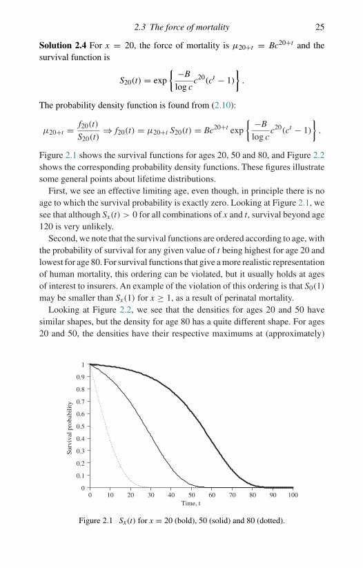
Solution 2.4 For x = 20, the force of mortality is µ20+t = Bc20+t and thesurvival function is
S20(t) = exp
{ −B
log cc20(ct − 1)
}.
The probability density function is found from (2.10):
µ20+t = f20(t)
S20(t)⇒ f20(t) = µ20+t S20(t) = Bc20+t exp
{ −B
log cc20(ct − 1)
}.
Figure 2.1 shows the survival functions for ages 20, 50 and 80, and Figure 2.2shows the corresponding probability density functions. These figures illustratesome general points about lifetime distributions.
First, we see an effective limiting age, even though, in principle there is noage to which the survival probability is exactly zero. Looking at Figure 2.1, wesee that although Sx(t) > 0 for all combinations of x and t, survival beyond age120 is very unlikely.
Second, we note that the survival functions are ordered according to age, withthe probability of survival for any given value of t being highest for age 20 andlowest for age 80. For survival functions that give a more realistic representationof human mortality, this ordering can be violated, but it usually holds at agesof interest to insurers. An example of the violation of this ordering is that S0(1)
may be smaller than Sx(1) for x ≥ 1, as a result of perinatal mortality.Looking at Figure 2.2, we see that the densities for ages 20 and 50 have
similar shapes, but the density for age 80 has a quite different shape. For ages20 and 50, the densities have their respective maximums at (approximately)
0
0.1
0.2
0.3
0.4
0.5
0.6
0.7
0.8
0.9
1
0 10 20 30 40 50 60 70 80 90 100Time, t
Surv
ival
pro
babi
lity
Figure 2.1 Sx(t) for x = 20 (bold), 50 (solid) and 80 (dotted).

26 Survival models
0
0.01
0.02
0.03
0.04
0.05
0.06
0.07
0 10 20 30 40 50 60 70 80 90 100Time, t
Figure 2.2 fx(t) for x = 20 (bold), 50 (solid) and 80 (dotted).
t = 60 and t = 30, indicating that death is most likely to occur around age80. The decreasing form of the density for age 80 also indicates that death ismore likely to occur at age 80 than at any other age for a life now aged 80. Afurther point to note about these density functions is that although each densityfunction is defined on (0, ∞), the spread of values of fx(t) is much greater forx = 20 than for x = 50, which, as we will see in Table 2.1, results in a greatervariance of future lifetime for x = 20 than for x = 50. �
2.4 Actuarial notation
The notation used in the previous sections, Sx(t), Fx(t) and fx(t), is standardin statistics. Actuarial science has developed its own notation, InternationalActuarial Notation, that encapsulates the probabilities and functions of greatestinterest and usefulness to actuaries. The force of mortality notation, µx, comesfrom International Actuarial Notation. We summarize the relevant actuarialnotation in this section, and rewrite the important results developed so far inthis chapter in terms of actuarial functions. The actuarial notation for survivaland mortality probabilities is
tpx = Pr[Tx > t] = Sx(t), (2.12)
tqx = Pr[Tx ≤ t] = 1 − Sx(t) = Fx(t), (2.13)
u|tqx = Pr[u < Tx ≤ u + t] = Sx(u) − Sx(u + t). (2.14)

2.4 Actuarial notation 27
So
• tpx is the probability that (x) survives to at least age x + t,• tqx is the probability that (x) dies before age x + t,• u|tqx is the probability that (x) survives u years, and then dies in the sub-
sequent t years, that is, between ages x + u and x + u + t. This is calleda deferred mortality probability, because it is the probability that deathoccurs in some interval following a deferred period.
We may drop the subscript t if its value is 1, so that px represents the probabilitythat (x) survives to at least age x + 1. Similarly, qx is the probability that (x)dies before age x + 1. In actuarial terminology qx is called the mortality rateat age x.
The relationships below follow immediately from the definitions above andthe previous results in this chapter:
tpx + tqx = 1,
u|tqx = upx − u+tpx,
t+upx = tpx upx+t from (2.5), (2.15)
µx = − 1
xp0
d
dxxp0 from (2.9). (2.16)
Similarly,
µx+t = − 1
tpx
d
dttpx ⇒ d
dttpx = −tpx µx+t , (2.17)
µx+t = fx(t)
Sx(t)⇒ fx(t) = tpx µx+t from (2.10), (2.18)
tpx = exp
{−∫ t
0µx+sds
}from (2.11). (2.19)
As Fx is a distribution function and fx is its density function, it follows that
Fx(t) =∫ t
0fx(s)ds,
which can be written in actuarial notation as
tqx =∫ t
0spx µx+sds. (2.20)
This is an important formula, which can be interpreted as follows. Considertime s, where 0 ≤ s < t. The probability that (x) is alive at time s is spx,
28 Survival models
Time 0
x
s
x+s
s+ds
x+s+ds
t
x+t
� �(x) survives s years
spx
� �
(x)dies
µx+sds
Age
Event
Probability
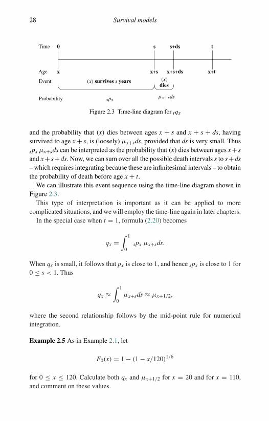
Figure 2.3 Time-line diagram for tqx
and the probability that (x) dies between ages x + s and x + s + ds, havingsurvived to age x + s, is (loosely) µx+sds, provided that ds is very small. Thus
spx µx+sds can be interpreted as the probability that (x) dies between ages x + sand x + s+ds. Now, we can sum over all the possible death intervals s to s+ds– which requires integrating because these are infinitesimal intervals – to obtainthe probability of death before age x + t.
We can illustrate this event sequence using the time-line diagram shown inFigure 2.3.
This type of interpretation is important as it can be applied to morecomplicated situations, and we will employ the time-line again in later chapters.
In the special case when t = 1, formula (2.20) becomes
qx =∫ 1
0spx µx+sds.
When qx is small, it follows that px is close to 1, and hence spx is close to 1 for0 ≤ s < 1. Thus
qx ≈∫ 1
0µx+sds ≈ µx+1/2,
where the second relationship follows by the mid-point rule for numericalintegration.
Example 2.5 As in Example 2.1, let
F0(x) = 1 − (1 − x/120)1/6
for 0 ≤ x ≤ 120. Calculate both qx and µx+1/2 for x = 20 and for x = 110,and comment on these values.

2.5 Mean and standard deviation of Tx 29
Solution 2.5 We have
px = S0(x + 1)
S0(x)=(
1 − 1
120 − x
)1/6
,
giving q20 = 0.00167 and q110 = 0.01741, and from the solution toExample 2.2, µ20 1
2= 0.00168 and µ110 1
2= 0.01754. We see that µx+1/2
is a good approximation to qx when the mortality rate is small, but is not sucha good approximation, at least in absolute terms, when the mortality rate is notclose to 0. �
2.5 Mean and standard deviation of Tx
Next, we consider the expected future lifetime of (x), E[Tx], denoted in actuarial
notation by◦ex. We also call this the complete expectation of life. In order to
evaluate◦ex, we note from formulae (2.17) and (2.18) that
fx(t) = tpx µx+t = − d
dttpx. (2.21)
From the definition of an expected value, we have
◦ex =
∫ ∞
0t fx(t)dt
=∫ ∞
0t tpx µx+tdt.
We can now use (2.21) to evaluate this integral using integration by parts as
◦ex = −
∫ ∞
0t
(d
dttpx
)dt
= −(
t tpx∣∣∞0 −
∫ ∞
0tpxdt
).
In Section 2.2 we stated the assumption that limt→∞ ttpx = 0, which gives
◦ex =
∫ ∞
0tpxdt. (2.22)
30 Survival models
Similarly, for E[T 2x ], we have
E[T 2x ] =
∫ ∞
0t2
tpx µx+tdt
= −∫ ∞
0t2(
d
dttpx
)dt
= −(
t2tpx
∣∣∣∞0
−∫ ∞
0tpx 2t dt
)
= 2∫ ∞
0t tpx dt. (2.23)
So we have integral expressions for E[Tx] and E[T 2x ]. For some lifetime distri-
butions we are able to integrate directly. In other cases we have to use numericalintegration techniques to evaluate the integrals in (2.22) and (2.23). The varianceof Tx can then be calculated as
V [Tx] = E[T 2
x
]−(◦
ex
)2.
Example 2.6 As in Example 2.1, let
F0(x) = 1 − (1 − x/120)1/6
for 0 ≤ x ≤ 120. Calculate◦ex and V[Tx] for (a) x = 30 and (b) x = 80.
Solution 2.6 As S0(x) = (1 − x/120)1/6, we have
tpx = S0(x + t)
S0(x)=(
1 − t
120 − x
)1/6
.
Now recall that this formula is valid for 0 ≤ t ≤ 120 − x, since under thismodel survival beyond age 120 is impossible. Technically, we have
tpx ={ (
1 − t120−x
)1/6for x + t ≤ 120,
0 for x + t > 120.
So the upper limit of integration in equation (2.22) is 120 − x, and
◦ex =
∫ 120−x
0
(1 − t
120 − x
)1/6
dt.

2.5 Mean and standard deviation of Tx 31
We make the substitution y = 1 − t/(120 − x), so that t = (120 − x)(1 − y),giving
◦ex = (120 − x)
∫ 1
0y1/6dy
= 67 (120 − x).
Then◦e30 = 77.143 and
◦e80 = 34.286.
Under this model the expectation of life at any age x is 6/7 of the time toage 120.
For the variance we require E[T 2x ]. Using equation (2.23) we have
E[T 2
x
]= 2
∫ 120−x
0t tpxdt
= 2∫ 120−x
0t
(1 − t
120 − x
)1/6
dt.
Again, we substitute y = 1 − t/(120 − x) giving
E[T 2
x
]= 2(120 − x)2
∫ 1
0(y1/6 − y7/6) dy
= 2(120 − x)2(
6
7− 6
13
).
Then
V[Tx] = E[T 2x ] −
(◦ex
)2 = (120 − x)2(
2(6/7 − 6/13) − (6/7)2)
= (120 − x)2 (0.056515) = ((120 − x) (0.23773))2 .
So V[T30] = 21.3962 and V[T80] = 9.5092.Since we know under this model that all lives will die before age 120, it
makes sense that the uncertainty in the future lifetime should be greater foryounger lives than for older lives. �
A feature of the model used in Example 2.6 is that we can obtain formulae for
quantities of interest such as◦ex, but for many models this is not possible. For
example, when we model mortality using Gompertz’ law, there is no explicit
formula for◦ex and we must use numerical integration to calculate moments of
Tx. In Appendix B we describe in detail how to do this.

32 Survival models
Table 2.1. Values of◦ex, SD[Tx] and expected
age at death for the Gompertz model withB = 0.0003 and c = 1.07.
x◦ex SD[Tx] x + ◦
ex
0 71.938 18.074 71.93810 62.223 17.579 72.22320 52.703 16.857 72.70330 43.492 15.841 73.49240 34.252 14.477 74.75250 26.691 12.746 76.69160 19.550 10.693 79.55070 13.555 8.449 83.55580 8.848 6.224 88.84890 5.433 4.246 95.433
100 3.152 2.682 103.152
Table 2.1 shows values of◦ex and the standard deviation of Tx (denoted
SD[Tx]) for a range of values of x using Gompertz’ law, µx = Bcx, whereB = 0.0003 and c = 1.07. For this survival model, 130p0 = 1.9 × 10⁻¹³, sothat using 130 as the maximum attainable age in our numerical integration isaccurate enough for practical purposes.
We see that◦ex is a decreasing function of x, as it was in Example 2.6. In
that example◦ex was a linear function of x, but we see that this is not true in
Table 2.1.
2.6 Curtate future lifetime
2.6.1 Kx and ex
In many insurance applications we are interested not only in the future lifetimeof an individual, but also in what is known as the individual’s curtate futurelifetime. The curtate future lifetime random variable is defined as the integerpart of future lifetime, and is denoted by Kx for a life aged x. If we let � denotethe floor function, we have
Kx = �Tx.
We can think of the curtate future lifetime as the number of whole years livedin the future by an individual. As an illustration of the importance of curtatefuture lifetime, consider the situation where a life aged x at time 0 is entitled topayments of 1 at times 1, 2, 3, . . . provided that (x) is alive at these times. Then
2.6 Curtate future lifetime 33
the number of payments made equals the number of complete years lived aftertime 0 by (x). This is the curtate future lifetime.
We can find the probability function of Kx by noting that for k = 0, 1, 2, . . .,Kx = k if and only if (x) dies between the ages of x + k and x + k + 1. Thusfor k = 0, 1, 2, . . .
Pr[Kx = k] = Pr[k ≤ Tx < k + 1]= k |qx
= kpx − k+1px
= kpx − kpx px+k
= kpx qx+k .
The expected value of Kx is denoted by ex, so that ex = E[Kx], and is referred toas the curtate expectation of life (even though it represents the expected curtatelifetime). So
E[Kx] = ex
=∞∑
k=0
k Pr[Kx = k]
=∞∑
k=0
k (kpx − k+1px)
= (1px − 2px) + 2(2px − 3px) + 3(3px − 4px) + · · ·
=∞∑
k=1
kpx. (2.24)
Note that the lower limit of summation is k = 1.Similarly,
E[K2x ] =
∞∑k=0
k2 ( kpx − k+1px)
= (1px − 2px) + 4(2px − 3px) + 9(3px − 4px) + 16(4px − 5px) + · · ·
= 2∞∑
k=1
k kpx −∞∑
k=1
kpx
= 2∞∑
k=1
k kpx − ex.
34 Survival models
As with the complete expectation of life, there are a few lifetime distributionsthat allow E[Kx] and E[K2
x ] to be calculated analytically. For more realisticmodels, such as Gompertz’, we can calculate the values easily using Excel orother suitable software. Although in principle we have to evaluate an infinitesum, at some age the survival probability will be sufficiently small that we cantreat it as an effective limiting age.
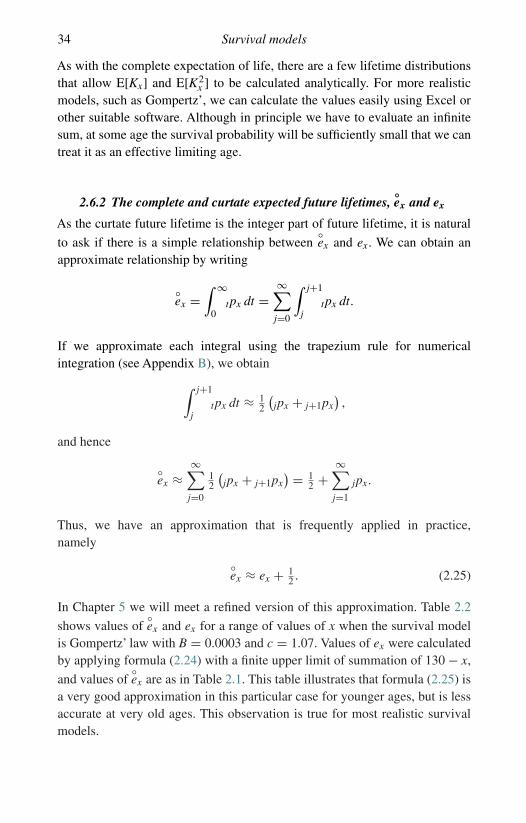
2.6.2 The complete and curtate expected future lifetimes,◦ex and ex
As the curtate future lifetime is the integer part of future lifetime, it is natural
to ask if there is a simple relationship between◦ex and ex. We can obtain an
approximate relationship by writing
◦ex =
∫ ∞
0tpx dt =
∞∑j=0
∫ j+1
jtpx dt.
If we approximate each integral using the trapezium rule for numericalintegration (see Appendix B), we obtain
∫ j+1
jtpx dt ≈ 1
2
(jpx + j+1px
),
and hence
◦ex ≈
∞∑j=0
12
(jpx + j+1px
) = 12 +
∞∑j=1
jpx.
Thus, we have an approximation that is frequently applied in practice,namely
◦ex ≈ ex + 1
2 . (2.25)
In Chapter 5 we will meet a refined version of this approximation. Table 2.2
shows values of◦ex and ex for a range of values of x when the survival model
is Gompertz’ law with B = 0.0003 and c = 1.07. Values of ex were calculatedby applying formula (2.24) with a finite upper limit of summation of 130 − x,
and values of◦ex are as in Table 2.1. This table illustrates that formula (2.25) is
a very good approximation in this particular case for younger ages, but is lessaccurate at very old ages. This observation is true for most realistic survivalmodels.

2.7 Notes and further reading 35
Table 2.2. Values of ex and◦ex for
Gompertz’ law with B = 0.0003and c = 1.07.
x ex◦ex
0 71.438 71.93810 61.723 62.22320 52.203 52.70330 42.992 43.49240 34.252 34.75250 26.192 26.69160 19.052 19.55070 13.058 13.55580 8.354 8.84890 4.944 5.433
100 2.673 3.152
2.7 Notes and further reading
Although laws of mortality such as Gompertz’ law are appealing due to theirsimplicity, they rarely represent mortality over the whole span of human ages.A simple extension of Gompertz’ law is Makeham’s law (Makeham, 1860),which models the force of mortality as
µx = A + Bcx. (2.26)
This is very similar to Gompertz’law, but adds a fixed term that is not age related,that allows better for accidental deaths. The extra term tends to improve the fitof the model to mortality data at younger ages.
In recent times, the Gompertz–Makeham approach has been generalizedfurther to give the GM(r, s) (Gompertz–Makeham) formula,
µx = h1r (x) + exp{h2
s (x)},
where h1r and h2
s are polynomials in x of degree r and s respectively. Adiscussionof this formula can be found in Forfar et al. (1988). Both Gompertz’ law andMakeham’s law are special cases of the GM formula.
In Section 2.3, we noted the importance of the force of mortality. A furthersignificant point is that when mortality data are analysed, the force of mortality

36 Survival models
is a natural quantity to estimate, whereas the lifetime distribution is not. Theanalysis of mortality data is a huge topic and is beyond the scope of this book.An excellent summary article on this topic is Macdonald (1996). For moregeneral distributions, the quantity f0(x)/S0(x), which actuaries call the forceof mortality at age x, is known as the hazard rate in survival analysis and thefailure rate in reliability theory.
2.8 Exercises
Exercise 2.1 Let F0(t) = 1 − (1 − t/105)1/5 for 0 ≤ t ≤ 105. Calculate
(a) the probability that a newborn life dies before age 60,(b) the probability that a life aged 30 survives to at least age 70,(c) the probability that a life aged 20 dies between ages 90 and 100,(d) the force of mortality at age 50,(e) the median future lifetime at age 50,(f) the complete expectation of life at age 50,(g) the curtate expectation of life at age 50.
Exercise 2.2 The function
G(x) = 18 000 − 110x − x2
18 000
has been proposed as the survival function S0(x) for a mortality model.
(a) What is the implied limiting age ω?(b) Verify that the function G satisfies the criteria for a survival function.(c) Calculate 20p0.(d) Determine the survival function for a life aged 20.(e) Calculate the probability that a life aged 20 will die between ages 30 and 40.(f) Calculate the force of mortality at age 50.
Exercise 2.3 Calculate the probability that a life aged 0 will die between ages19 and 36, given the survival function
S0(x) = 1
10
√100 − x, 0 ≤ x ≤ 100 (= ω).
Exercise 2.4 Let
S0(x) = exp
{−(
Ax + 1
2Bx2 + C
log DDx − C
log D
)}
where A, B, C and D are all positive.
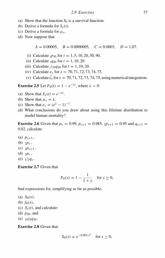
2.8 Exercises 37
(a) Show that the function S0 is a survival function.(b) Derive a formula for Sx(t).(c) Derive a formula for µx.(d) Now suppose that
A = 0.00005, B = 0.0000005, C = 0.0003, D = 1.07.
(i) Calculate tp30 for t = 1, 5, 10, 20, 50, 90.(ii) Calculate tq40 for t = 1, 10, 20.
(iii) Calculate t |10q30 for t = 1, 10, 20.(iv) Calculate ex for x = 70, 71, 72, 73, 74, 75.
(v) Calculate◦ex for x = 70, 71, 72, 73, 74, 75, using numerical integration.
Exercise 2.5 Let F0(t) = 1 − e−λt , where λ > 0.
(a) Show that Sx(t) = e−λt .(b) Show that µx = λ.(c) Show that ex = (eλ − 1)−1.(d) What conclusions do you draw about using this lifetime distribution to
model human mortality?
Exercise 2.6 Given that px = 0.99, px+1 = 0.985, 3px+1 = 0.95 and qx+3 =0.02, calculate
(a) px+3 ,(b) 2px ,(c) 2px+1 ,(d) 3px ,(e) 1|2qx .
Exercise 2.7 Given that
F0(x) = 1 − 1
1 + xfor x ≥ 0,
find expressions for, simplifying as far as possible,
(a) S0(x),(b) f0(x),(c) Sx(t), and calculate:(d) p20, and(e) 10|5q30.
Exercise 2.8 Given that
S0(x) = e−0.001 x2for x ≥ 0,

38 Survival models
find expressions for, simplifying as far as possible,
(a) f0(x), and(b) µx.
Exercise 2.9 Show that
d
dxtpx = tpx (µx − µx+t) .
Exercise 2.10 Suppose that Gompertz’ law applies with µ30 = 0.000130 andµ50 = 0.000344. Calculate 10p40.
Exercise 2.11 A survival model follows Makeham’s law, so that
µx = A + Bcx for x ≥ 0.
(a) Show that under Makeham’s law
tpx = stgcx(ct−1), (2.27)
where s = e−A and g = exp{−B/ log c}.(b) Suppose you are given the values of 10p50, 10p60 and 10p70. Show that
c =(
log( 10p70) − log( 10p60)
log( 10p60) − log( 10p50)
)0.1
.
Exercise 2.12 (a) Construct a table of px for Makeham’s law with parametersA = 0.0001, B = 0.00035 and c = 1.075, for integer x from age 0 to age130, using Excel or other appropriate computer software. You should setthe parameters so that they can be easily changed, and you should keep thetable, as many exercises and examples in future chapters will use it.
(b) Use the table to determine the age last birthday at which a life currentlyaged 70 is most likely to die.
(c) Use the table to calculate e70.
(d) Using a numerical approach, calculate◦e70.
Exercise 2.13 A life insurer assumes that the force of mortality of smokers atall ages is twice the force of mortality of non-smokers.
(a) Show that, if * represents smokers’ mortality, and the ‘unstarred’ functionrepresents non-smokers’ mortality, then
tp∗x = (tpx)
2 .

2.8 Exercises 39
(b) Calculate the difference between the life expectancy of smokers and non-smokers aged 50, assuming that non-smokers mortality follows Gompertz’law, with B = 0.0005 and c = 1.07.
(c) Calculate the variance of the future lifetime for a non-smoker aged 50 andfor a smoker aged 50 under Gompertz’ law.
Hint: You will need to use numerical integration for parts (b) and (c).
Exercise 2.14 (a) Show that
◦ex ≤ ◦
ex+1 + 1.
(b) Show that
◦ex ≥ ex.
(c) Explain (in words) why
◦ex ≈ ex + 1
2.
(d) Is◦ex always a non-increasing function of x?
Exercise 2.15 (a) Show that
oex = 1
S0(x)
∫ ∞
xS0(t)dt,
where S0(t) = 1 − F0(t), and hence, or otherwise, prove that
d
dxoex = µx
oex − 1.
Hint:d
dx
{∫ x
ag(t)dt
}= g(x). What about
d
dx
{∫ a
xg(t)dt
}?
(b) Deduce that
x + oex
is an increasing function of x, and explain this result intuitively.
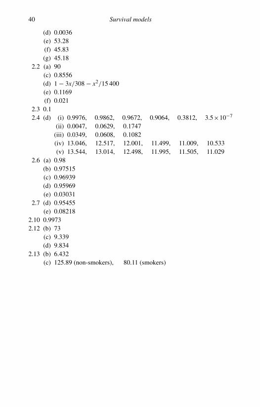
Answers to selected exercises
2.1 (a) 0.1559(b) 0.8586(c) 0.1394
40 Survival models
(d) 0.0036(e) 53.28(f) 45.83(g) 45.18
2.2 (a) 90(c) 0.8556(d) 1 − 3x/308 − x2/15 400(e) 0.1169(f) 0.021
2.3 0.12.4 (d) (i) 0.9976, 0.9862, 0.9672, 0.9064, 0.3812, 3.5×10⁻⁷
(ii) 0.0047, 0.0629, 0.1747(iii) 0.0349, 0.0608, 0.1082(iv) 13.046, 12.517, 12.001, 11.499, 11.009, 10.533(v) 13.544, 13.014, 12.498, 11.995, 11.505, 11.029
2.6 (a) 0.98(b) 0.97515(c) 0.96939(d) 0.95969(e) 0.03031
2.7 (d) 0.95455(e) 0.08218
2.10 0.99732.12 (b) 73
(c) 9.339(d) 9.834
2.13 (b) 6.432(c) 125.89 (non-smokers), 80.11 (smokers)

3
Life tables and selection
3.1 Summary
In this chapter we define a life table. For a life table tabulated at integer agesonly, we show, using fractional age assumptions, how to calculate survivalprobabilities for all ages and durations.
We discuss some features of national life tables from Australia, England &Wales and the United States.
We then consider life tables appropriate to individuals who have purchasedparticular types of life insurance policy and discuss why the survival probabil-ities differ from those in the corresponding national life table. We consider theeffect of ‘selection’of lives for insurance policies, for example through medicalunderwriting. We define a select survival model and we derive some formulaefor such a model.
3.2 Life tables
Given a survival model, with survival probabilities tpx, we can construct the lifetable for the model from some initial age x0 to a maximum age ω. We define afunction {lx} for x0 ≤ x ≤ ω as follows. Let lx0 be an arbitrary positive number(called the radix of the table) and, for 0 ≤ t ≤ ω − x0, define
lx0+t = lx0 tpx0 .
From this definition we see that for x0 ≤ x ≤ x + t ≤ ω,
lx+t = lx0 x+t−x0 px0
= lx0 x−x0 px0 tpx
= lx tpx ,
41

42 Life tables and selection
so that
tpx = lx+t/lx. (3.1)
For any x ≥ x0, we can interpret lx+t as the expected number of survivors toage x + t out of lx independent individuals aged x. This interpretation is morenatural if lx is an integer, and follows because the number of survivors to agex + t is a random variable with a binomial distribution with parameters lx and
tpx. That is, suppose we have lx independent lives aged x, and each life has aprobability tpx of surviving to age x + t. Then the number of survivors to agex + t is a binomial random variable, Lt , say, with parameters lx and tpx. Theexpected value of the number of survivors is then
E[Lt] = lx tpx = lx+t .
We always use the table in the form ly/lx which is why the radix of the table isarbitrary – it would make no difference to the survival model if all the lx valueswere multiplied by 100, for example.
From (3.1) we can use the lx function to calculate survival probabilities. Wecan also calculate mortality probabilities. For example,
q30 = 1 − l31
l30= l30 − l31
l30(3.2)
and
15|30q40 = 15p40 30q55 = l55
l40
(1 − l85
l55
)= l55 − l85
l40. (3.3)
In principle, a life table is defined for all x from the initial age, x0, to the limitingage, ω. In practice, it is very common for a life table to be presented, and insome cases even defined, at integer ages only. In this form, the life table is auseful way of summarizing a lifetime distribution since, with a single columnof numbers, it allows us to calculate probabilities of surviving or dying overinteger numbers of years starting from an integer age.
It is usual for a life table, tabulated at integer ages, to show the values of dx,where
dx = lx − lx+1, (3.4)
in addition to lx, as these are used to compute qx. From (3.4) we have
dx = lx
(1 − lx+1
lx
)= lx(1 − px) = lx qx.
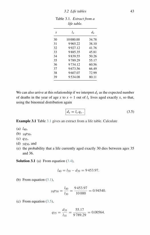
3.2 Life tables 43
Table 3.1. Extract from alife table.
x lx dx
30 10 000.00 34.7831 9 965.22 38.1032 9 927.12 41.7633 9 885.35 45.8134 9 839.55 50.2635 9 789.29 55.1736 9 734.12 60.5637 9 673.56 66.4938 9 607.07 72.9939 9 534.08 80.11
We can also arrive at this relationship if we interpret dx as the expected numberof deaths in the year of age x to x + 1 out of lx lives aged exactly x, so that,using the binomial distribution again
dx = lx qx . (3.5)
Example 3.1 Table 3.1 gives an extract from a life table. Calculate
(a) l40,(b) 10p30,(c) q35,(d) 5q30, and(e) the probability that a life currently aged exactly 30 dies between ages 35
and 36.
Solution 3.1 (a) From equation (3.4),
l40 = l39 − d39 = 9 453.97.
(b) From equation (3.1),
10p30 = l40
l30= 9 453.97
10 000= 0.94540.
(c) From equation (3.5),
q35 = d35
l35= 55.17
9 789.29= 0.00564.
44 Life tables and selection
(d) Following equation (3.2),
5q30 = l30 − l35
l30= 0.02107.
(e) This probability is 5| q30. Following equation (3.3),
5| q30 = l35 − l36
l30= d35
l30= 0.00552.
�
3.3 Fractional age assumptions
A life table {lx}x≥x0 provides exactly the same information as the correspondingsurvival distribution, Sx0 . However, a life table tabulated at integer ages onlydoes not contain all the information in the corresponding survival model, sincevalues of lx at integer ages x are not sufficient to be able to calculate probabili-ties involving non-integer ages, such as 0.75p30.5. Given values of lx at integerages only, we need an additional assumption or some further information to cal-culate probabilities for non-integer ages or durations. Specifically, we need tomake some assumption about the probability distribution for the future lifetimerandom variable between integer ages.
We use the term fractional age assumption to describe such an assumption.It may be specified in terms of the force of mortality function or the survival ormortality probabilities.
In this section we assume that a life table is specified at integer ages only andwe describe the two most useful fractional age assumptions.
3.3.1 Uniform distribution of deaths
The uniform distribution of deaths (UDD) assumption is the most commonfractional age assumption. It can be formulated in two different, but equivalent,ways as follows.
UDD1For integer x, and for 0 ≤ s < 1, assume that
sqx = sqx . (3.6)
UDD2Recall from Chapter 2 that Kx is the integer part of Tx, and define a new
random variable Rx such that
Tx = Kx + Rx.
3.3 Fractional age assumptions 45
The UDD2 assumption is that, for integer x, Rx ∼ U(0, 1), and Rx isindependent of Kx.
The equivalence of these two assumptions is demonstrated as follows. First,assume that UDD1 is true. Then for integer x, and for 0 ≤ s < 1,
Pr[Rx ≤ s] =∞∑
k=0
Pr[Rx ≤ s and Kx = k]
=∞∑
k=0
Pr[k ≤ Tx ≤ k + s]
=∞∑
k=0
kpx sqx+k
=∞∑
k=0
kpx s (qx+k) using UDD1
= s∞∑
k=0
kpx qx+k
= s∞∑
k=0
Pr[Kx = k]
= s.
This proves that Rx ∼ U(0, 1). To prove the independence of Rx and Kx,note that
Pr[Rx ≤ s and Kx = k] = Pr[k ≤ Tx ≤ k + s]= kpx sqx+k
= s kpx qx+k
= Pr[Rx ≤ s] Pr[Kx = k]
since Rx ∼ U(0, 1). This proves that UDD1 implies UDD2.To prove the reverse implication, assume that UDD2 is true. Then for
integer x, and for 0 ≤ s < 1,
sqx = Pr[Tx ≤ s]= Pr[Kx = 0 and Rx ≤ s]= Pr[Rx ≤ s] Pr[Kx = 0]

46 Life tables and selection
as Kx and Rx are assumed independent. Thus,
sqx = s qx . (3.7)
Formulation UDD2 explains why this assumption is called the Uniform Distri-bution of Deaths, but in practical applications of this assumption, formulationUDD1 is the more useful of the two.
An immediate consequence is that
lx+s = lx − s dx (3.8)
for 0 ≤ s < 1. This follows because
sqx = 1 − lx+s
lx
and substituting s qx for sqx gives
sdx
lx= lx − lx+s
lx.
Hence
lx+s = lx − s dx
for 0 ≤ s ≤ 1. Thus, we assume that lx+s is a linearly decreasing function of s.Differentiating equation (3.6) with respect to s, we obtain
d
dssqx = qx, 0 ≤ s ≤ 1
and we know that the left-hand side is the probability density function for Tx
at s, because we are differentiating the distribution function. The probabilitydensity function for Tx at s is spx µx+s so that under UDD
qx = spx µx+s (3.9)
for 0 ≤ s < 1.The left-hand side does not depend on s, which means that the density function
is a constant for 0 ≤ s < 1, which also follows from the uniform distributionassumption for Rx.
Since qx is constant with respect to x, and spx is a decreasing function ofs, we can see that µx+s is an increasing function of s, which is appropriatefor ages of interest to insurers. However, if we apply the approximation oversuccessive ages, we obtain a discontinuous function for the force of mortality,

3.3 Fractional age assumptions 47
with discontinuities occurring at integer ages, as illustrated in Example 3.4.Although this is undesirable, it is not a serious drawback.
Example 3.2 Given that p40 = 0.999473, calculate 0.4q40.2 under theassumption of a uniform distribution of deaths.
Solution 3.2 We note that the fundamental result in equation (3.7), that forfractional of a year s, sqx = s qx, requires x to be an integer. We can manipulatethe required probability 0.4q40.2 to involve only probabilities from integer agesas follows
0.4q40.2 = 1 − 0.4p40.2 = 1 − l40.6
l40.2
= 1 − 0.6p40
0.2p40= 1 − 1 − 0.6q40
1 − 0.2q40
= 2.108 × 10⁻⁴.
�
Example 3.3 Use the life table in Example 3.1 above, with the UDDassumption, to calculate (a) 1.7q33 and (b) 1.7q33.5.
Solution 3.3 (a) We note first that
1.7q33 = 1 − 1.7p33 = 1 − (p33) (0.7p34).
We can calculate p33 directly from the life table as l34/l33 = 0.995367 and
0.7p34 = 1 − 0.7 q34 = 0.996424 under UDD, so that 1.7q33 = 0.008192.(b) To calculate 1.7q33.5 using UDD, we express this as
1.7q33.5 = 1 − 1.7p33.5
= 1 − l35.2
l33.5
= 1 − l35 − 0.2d35
l33 − 0.5d33
= 0.008537.
�
Example 3.4 Under the assumption of a uniform distribution of deaths, cal-culate lim
t→1− µ40+t using p40 = 0.999473, and calculate limt→0+ µ41+t using
p41 = 0.999429.
48 Life tables and selection
Solution 3.4 From formula (3.9), we have µx+t = qx/tpx. Setting x = 40yields
limt→1− µ40+t = q40/p40 = 5.273 × 10⁻⁴,
while setting x = 41 yields
limt→0+ µ41+t = q41 = 5.71 × 10⁻⁴.
�
Example 3.5 Given that q70 = 0.010413 and q71 = 0.011670, calculate 0.7q70.6
assuming a uniform distribution of deaths.
Solution 3.5 As deaths are assumed to be uniformly distributed between ages70 to 71 and ages 71 to 72, we write
0.7q70.6 = 0.4q70.6 + (1 − 0.4q70.6) 0.3q71.
Following the same arguments as in Solution 3.3, we obtain
0.4q70.6 = 1 − 1 − q70
1 − 0.6q70= 4.191 × 10⁻³,
and as 0.3q71 = 0.3q71 = 3.501 × 10⁻³, we obtain 0.7q70.6 = 7.678 × 10⁻³. �
3.3.2 Constant force of mortality
A second fractional age assumption is that the force of mortality is constantbetween integer ages. Thus, for integer x and 0 ≤ s < 1, we assume that µx+s
does not depend on s, and we denote it µ∗x . We can obtain the value of µ∗
x byusing the fact that
px = exp
{−∫ 1
0µx+sds
}.
Hence the assumption that µx+s = µ∗x for 0 ≤ s < 1 gives px = e−µ∗
x orµ∗
x = − log px. Further, under the assumption of a constant force of mortality,for 0 ≤ s < 1 we obtain
spx = exp
{−∫ s
0µ∗
x du
}= e−µ∗
x s = (px)s.
Similarly, for t, s > 0 and t + s < 1,
spx+t = exp
{−∫ s
0µ∗
x du
}= (px)
s.

3.4 National life tables 49
Thus, under the constant force assumption, the probability of surviving for aperiod of s < 1 years from age x + t is independent of t provided that s+ t < 1.
The assumption of a constant force of mortality leads to a step function forthe force of mortality over successive years of age. By its nature, the assumptionproduces a constant force of mortality over the year of age x to x + 1, whereaswe would expect the force of mortality to increase for most ages. However, ifthe true force of mortality increases slowly over the year of age, the constantforce of mortality assumption is reasonable.
Example 3.6 Given that p40 = 0.999473, calculate 0.4q40.2 under theassumption of a constant force of mortality.
Solution 3.6 We have 0.4q40.2 = 1 − 0.4p40.2 = 1 − (p40)0.4 = 2.108 × 10⁻⁴.
�
Example 3.7 Given that q70 = 0.010413 and q71 = 0.011670, calculate 0.7q70.6
under the assumption of a constant force of mortality.
Solution 3.7 As in Solution 3.5 we write
0.7q70.6 = 0.4q70.6 + (1 − 0.4q70.6) 0.3q71,
where 0.4q70.6 = 1 − (p70)0.4 = 4.178 × 10⁻³ and 0.3q71 = 1 − (p71)
0.3 =3.515 × 10⁻³, giving 0.7q70.6 = 7.679 × 10⁻³. �
Note that in Examples 3.2 and 3.5 and in Examples 3.6 and 3.7 we have used twodifferent methods to solve the same problems, and the solutions agree to fivedecimal places. It is generally true that the assumptions of a uniform distributionof deaths and a constant force of mortality produce very similar solutions toproblems. The reason for this can be seen from the following approximations.Under the constant force of mortality assumption
qx = 1 − e−µ∗ ≈ µ∗
provided that µ∗ is small, and for 0 < t < 1,
tqx = 1 − e−µ∗t ≈ µ∗t.
In other words, the approximation to tqx is t times the approximation to qx,which is what we obtain under the uniform distribution of deaths assumption.
3.4 National life tables
Life tables based on the mortality experience of the whole population of acountry are regularly produced for many countries in the world. Separate life

50 Life tables and selection
Table 3.2. Values of qx × 105 from some national life tables.
Australian Life Tables2000–02
English Life Table 151990–92
US Life Tables2002
x Males Females Males Females Males Females
0 567 466 814 632 764 6271 44 43 62 55 53 422 31 19 38 30 37 28
10 13 8 18 13 18 1320 96 36 84 31 139 4530 119 45 91 43 141 6340 159 88 172 107 266 14950 315 202 464 294 570 31960 848 510 1 392 830 1 210 75870 2 337 1 308 3 930 2 190 2 922 1 89980 6 399 4 036 9 616 5 961 7 028 4 93090 15 934 12 579 20 465 15 550 16 805 13 328
100 24 479 23 863 38 705 32 489 − −
tables are usually produced for males and for females and possibly for someother groups of individuals, for example on the basis of smoking habits.
Table 3.2 shows values of qx × 105, where qx is the probability of dyingwithin one year, for selected ages x, separately for males and females, for thepopulations of Australia, England & Wales and the United States. These tablesare constructed using records of deaths in a particular year, or a small number ofconsecutive years, and estimates of the population in the middle of that period.The relevant years are indicated in the column headings for each of the threelife tables in Table 3.2. Data at the oldest ages are notoriously unreliable. Forthis reason, the United States Life Tables do not show values of qx for ages 100and higher.
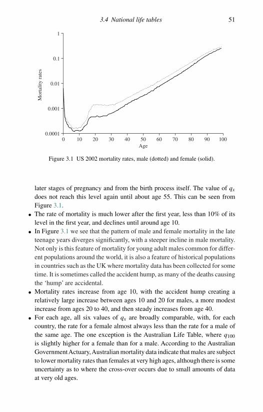
For all three national life tables and for both males and females, the valuesof qx follow exactly the same pattern as a function of age, x. Figure 3.1 showsthe US 2002 mortality rates for males and females; the graphs for England& Wales and for Australia are similar. (Note that we have plotted these ona logarithmic scale in order to highlight the main features. Also, although theinformation plotted consists of values of qx for x = 0, 1, . . . , 99, we have plotteda continuous line as this gives a clearer representation.) We note the followingpoints from Table 3.2 and Figure 3.1.
• The value of q0 is relatively high. Mortality rates immediately followingbirth, perinatal mortality, are high due to complications arising from the
3.4 National life tables 51
0.0001
0.001
0.01
0.1
1
0 10 20 30 40 50 60 70 80 90 100Age
Mor
talit
y ra
tes
Figure 3.1 US 2002 mortality rates, male (dotted) and female (solid).
later stages of pregnancy and from the birth process itself. The value of qx
does not reach this level again until about age 55. This can be seen fromFigure 3.1.
• The rate of mortality is much lower after the first year, less than 10% of itslevel in the first year, and declines until around age 10.
• In Figure 3.1 we see that the pattern of male and female mortality in the lateteenage years diverges significantly, with a steeper incline in male mortality.Not only is this feature of mortality for young adult males common for differ-ent populations around the world, it is also a feature of historical populationsin countries such as the UK where mortality data has been collected for sometime. It is sometimes called the accident hump, as many of the deaths causingthe ‘hump’ are accidental.
• Mortality rates increase from age 10, with the accident hump creating arelatively large increase between ages 10 and 20 for males, a more modestincrease from ages 20 to 40, and then steady increases from age 40.
• For each age, all six values of qx are broadly comparable, with, for eachcountry, the rate for a female almost always less than the rate for a male ofthe same age. The one exception is the Australian Life Table, where q100
is slightly higher for a female than for a male. According to the AustralianGovernmentActuary,Australian mortality data indicate that males are subjectto lower mortality rates than females at very high ages, although there is someuncertainty as to where the cross-over occurs due to small amounts of dataat very old ages.

52 Life tables and selection
0.00
0.05
0.10
0.15
0.20
0.25
0.30
0.35
50 60 70 80 90 100Age
Mor
talit
y ra
tes
Figure 3.2 US 2002 male mortality rates (solid), with fitted Gompertz mortality rates(dotted).
• The Gompertz model introduced in Chapter 2 is relatively simple, in thatit requires only two parameters and has a force of mortality with a simplefunctional form, µx = Bcx. We stated in Chapter 2 that this model doesnot provide a good fit across all ages. We can see from Figure 3.1 that themodel cannot fit the perinatal mortality, nor the accident hump. However,the mortality rates at later ages are rather better behaved, and the Gompertzmodel often proves useful over older age ranges. Figure 3.2 shows the olderages US 2002 Males mortality rate curve, along with a Gompertz curve fittedto the US 2002 Table mortality rates. The Gompertz curve provides a prettyclose fit – which is a particularly impressive feat, considering that Gompertzproposed the model in 1825.
A final point about Table 3.2 is that we have compared three national life tablesusing values of the probability of dying within one year, qx, rather than theforce of mortality, µx. This is because values of µx are not published for anyages for the US Life Tables. Also, values of µx are not published for age 0 forthe other two life tables – there are technical difficulties in the estimation ofµx within a year in which the force of mortality is changing rapidly, as it doesbetween ages 0 and 1.
3.5 Survival models for life insurance policyholders
Suppose we have to choose a survival model appropriate for a man, currentlyaged 50 and living in the UK, who has just purchased a 10-year term insurance

3.5 Survival models for life insurance policyholders 53
Table 3.3. Values of the force of mortality ×105
from English Life Table 15 and CMI (Table A14)for UK males who purchase a term insurance
policy at age 50.
x ELTM 15 CMI
50 440 7852 549 15254 679 24056 845 36058 1057 45460 1323 573
policy. We could use a national life table, say English Life Table 15, so that,for example, we could assume that the probability this man dies before age51 is 0.00464, as shown in Table 3.2. However, in the UK, as in some othercountries with well-developed life insurance markets, the mortality experienceof people who purchase life insurance policies tends to be different from thepopulation as a whole. The mortality of different types of life insurance policy-holders is investigated separately, and life tables appropriate for these groupsare published.
Table 3.3 shows values of the force of mortality (×105) at two-year intervalsfrom age 50 to age 60 taken from English Life Table 15, Males (ELTM 15), andfrom a life table prepared from data relating to term insurance policyholdersin the UK in 1999–2002 and which assumes the policyholders purchased theirpolicies at age 50. This second set of mortality rates come from Table A14 ofa 2006 working paper of the Continuous Mortality Investigation in the UK.Hereafter we refer to this working paper as CMI, and further details are givenat the end of this chapter. The values of the force of mortality for ELTM 15correspond to the values of qx shown in Table 3.2.
The striking feature of Table 3.3 is the difference between the two sets ofvalues. The values from CMI are very much lower than those from ELTM 15,by a factor of more than 5 at age 50 and by a factor of more than 2 at age 60.There are at least three reasons for this difference. Two of these are discussedbelow, the third is discussed in the next section.
(a) The data on which the two life tables are based relate to different calendaryears; 1990–92 in the case of ELTM 15 and 1999–2002 in the case of CMI.Mortality rates in the UK, as in many other countries, have been decreasingfor some years so we might expect rates based on more recent data to be

54 Life tables and selection
lower. However, this explains only a small part of the differences in Table3.3.An interim life table for England &Wales based on population data from2002–2004, gives the following values for males: µ50 = 391 × 10−5 andµ60 = 1008 × 10−5. Clearly, mortality in England & Wales has improvedover the 12-year period, but not to the extent that it matches the CMI valuesshown in Table 3.3. Other explanations for the differences in Table 3.3 areneeded.
(b) A major reason for the difference between the values in Table 3.3 is thatELTM 15 is a life table based on the whole male population of England& Wales, whereas CMI (Table A14) is based on the experience of maleswho are term insurance policyholders. Within any large group, there arelikely to be variations in mortality rates between subgroups. This is truein the case of the population of England and Wales, where social class,defined in terms of occupation, has a significant effect on mortality. Putsimply, the better your job, and hence the wealthier you are likely to be, thelower your mortality rates. Given that people who purchase term insurancepolicies are likely to be among the better paid people in the population, wehave an explanation for a large part of the difference between the values inTable 3.3.
CMI (TableA2) shows values of the force of mortality based on data from malesin the UK who purchased whole life or endowment insurance policies. These aresimilar to those shown in Table 3.3 for term insurance policyholders and hencemuch lower than the values for the whole population. People who purchasewhole life or endowment policies, like those who purchase term insurancepolicies, tend to be among the wealthier people in the population.
3.6 Life insurance underwriting
The values of the force of mortality in Table 3.3 taken from CMI are valuesbased on data for males who purchased term insurance at age 50. CMI (TableA14) gives values for different ages at the purchase of the policy ranging from17 to 90. Values for ages at purchase 50, 52, 54 and 56 are shown in Table 3.4.
There are two significant features of the values in Table 3.4, which can beseen by considering the rows of values for ages 56 and 62.
(a) Consider the row of values for age 56. Each of the four values in thisrow is the force of mortality at age 56 based on data from the UK overthe period 1999–2002 for males who are term insurance policyholders.The only difference is that they purchased their policies at different ages.The more recently the policy was purchased, the lower the force of mortal-ity. For example, for a male who purchased his policy at age 56, the value
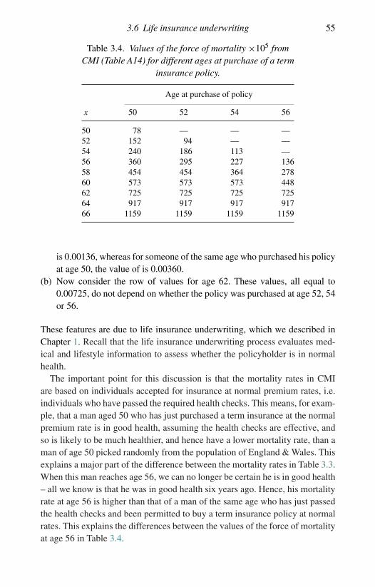
3.6 Life insurance underwriting 55
Table 3.4. Values of the force of mortality ×105 fromCMI (Table A14) for different ages at purchase of a term
insurance policy.
Age at purchase of policy
x 50 52 54 56
50 78 — — —52 152 94 — —54 240 186 113 —56 360 295 227 13658 454 454 364 27860 573 573 573 44862 725 725 725 72564 917 917 917 91766 1159 1159 1159 1159
is 0.00136, whereas for someone of the same age who purchased his policyat age 50, the value of is 0.00360.
(b) Now consider the row of values for age 62. These values, all equal to0.00725, do not depend on whether the policy was purchased at age 52, 54or 56.
These features are due to life insurance underwriting, which we described inChapter 1. Recall that the life insurance underwriting process evaluates med-ical and lifestyle information to assess whether the policyholder is in normalhealth.
The important point for this discussion is that the mortality rates in CMIare based on individuals accepted for insurance at normal premium rates, i.e.individuals who have passed the required health checks. This means, for exam-ple, that a man aged 50 who has just purchased a term insurance at the normalpremium rate is in good health, assuming the health checks are effective, andso is likely to be much healthier, and hence have a lower mortality rate, than aman of age 50 picked randomly from the population of England & Wales. Thisexplains a major part of the difference between the mortality rates in Table 3.3.When this man reaches age 56, we can no longer be certain he is in good health– all we know is that he was in good health six years ago. Hence, his mortalityrate at age 56 is higher than that of a man of the same age who has just passedthe health checks and been permitted to buy a term insurance policy at normalrates. This explains the differences between the values of the force of mortalityat age 56 in Table 3.4.
56 Life tables and selection
The effect of passing the health checks at an earlier age eventually wearsoff, so that at age 62, the force of mortality does not depend on whether thepolicy was purchased at age 52, 54 or 56. This is point (b) above. However,note that these rates, 0.00725, are still much lower than µ62 (= 0.01664) fromELTM 15. This is because people who buy insurance tend, at least in the UK, tohave lower mortality than the general population. In fact the population is madeup of many heterogeneous lives, and the effect of initial selection is only onearea where actuaries have tried to manage the heterogeneity. In the US, therehas been a lot of activity recently developing tables for ‘preferred lives’, whoare assumed to be even healthier than the standard insured population. Thesepreferred lives tend to be from higher socio-economic groups. Mortality andwealth are closely linked.
3.7 Select and ultimate survival models
A feature of the survival models studied in Chapter 2 is that probabilities offuture survival depend only on the individual’s current age. For example, for agiven survival model and a given term t, tpx, the probability that an individualcurrently aged x will survive to age x + t, depends only on the current age x.Such survival models are called aggregate survival models, because lives areall aggregated together.
The difference between an aggregate survival model and the survival modelfor term insurance policyholders discussed in Section 3.6 is that in the lattercase, probabilities of future survival depend not only on current age but also onhow long ago the individual entered the group of policyholders, i.e. when thepolicy was purchased.
This leads us to the following definition. The mortality of a group of individ-uals is described by a select and ultimate survival model, usually shortenedto select survival model, if the following statements are true.
(a) Future survival probabilities for an individual in the group depend on theindividual’s current age and on the age at which the individual joined thegroup.
(b) There is a positive number (generally an integer), which we denote by d ,such that if an individual joined the group more than d years ago, futuresurvival probabilities depend only on current age. The initial selection effectis assumed to have worn off after d years.
We use the following terminology for a select survival model. An individualwho enters the group at, say, age x, is said to be selected, or just select, at agex. The period d after which the age at selection has no effect on future survival
3.7 Select and ultimate survival models 57
probabilities is called the select period for the model. The mortality that appliesto lives after the select period is complete is called the ultimate mortality, sothat the complete model comprises a select period followed by the ultimateperiod.
Going back to the term insurance policyholders in Section 3.6, we can identifythe ‘group’ as male term insurance policyholders in the UK. A select survivalmodel is appropriate in this case because passing the health checks at age xindicates that the individual is in good health and so has lower mortality ratesthan someone of the same age who passed these checks some years ago. Thereare indications in Table 3.4 that the select period, d , for this group is less than orequal to six years. See point (b) in Section 3.6. In fact, the select period is fiveyears for this particular model. Select periods typically range from one year to15 years for life insurance mortality models.
For the term insurance policyholders in Section 3.6, being selected at age xmeant that the mortality rate for the individual was lower than that of a terminsurance policyholder of the same age who had been selected some yearsearlier. Selection can occur in many different ways and does not always lead tolower mortality rates, as Example 3.8 shows.
Example 3.8 Consider men who need to undergo surgery because they aresuffering from a particular disease. The surgery is complicated and there is aprobability of only 50% that they will survive for a year following surgery. Ifthey do survive for a year, then they are fully cured and their future mortalityfollows the Australian Life Tables 2000–02, Males, from which you are giventhe following values:
l60 = 89 777, l61 = 89 015, l70 = 77 946.
Calculate
(a) the probability that a man aged 60 who is just about to have surgery willbe alive at age 70,
(b) the probability that a man aged 60 who had surgery at age 59 will be aliveat age 70, and
(c) the probability that a man aged 60 who had surgery at age 58 will be aliveat age 70.
Solution 3.8 In this example, the ‘group’is all men who have had the operation.Being selected at age x means having surgery at age x. The select period of thesurvival model for this group is one year, since if they survive for one year afterbeing ‘selected’, their future mortality depends only on their current age.

58 Life tables and selection
(a) The probability of surviving to age 61 is 0.5. Given that he survives to age61, the probability of surviving to age 70 is
l70/l61 = 77 946/89 015 = 0.8757.
Hence, the probability that this individual survives from age 60 to age 70 is
0.5 × 0.8757 = 0.4378.
(b) Since this individual has already survived for one year following surgery,his mortality follows the Australian Life Tables 2000–02, Males. Hence,his probability of surviving to age 70 is
l70/l60 = 77 946/89 777 = 0.8682.
(c) Since this individual’s surgery was more than one year ago, his futuremortality is exactly the same, probabilistically, as the individual in part (b).Hence, his probability of surviving to age 70 is 0.8682. �
Selection is not a feature of national life tables since, ignoring immigration, anindividual can enter the population only at age zero. It is an important featureof many survival models based on data from, and hence appropriate to, lifeinsurance policyholders. We can see from Tables 3.3 and 3.4 that its effect onthe force of mortality can be considerable. For these reasons, select survivalmodels are important in life insurance mathematics.
The select period may be different for different survival models. For CMI(Table A14), which relates to term insurance policyholders, it is five years, asnoted above; for CMI (Table A2), which relates to whole life and endowmentpolicyholders, the select period is two years.
In the next section we introduce notation and develop some formulae forselect survival models.
3.8 Notation and formulae for select survival models
A select survival model represents an extension of the ultimate survival modelstudied in Chapter 2. In Chapter 2, survival probabilities depended only onthe current age of the individual. For a select survival model, probabilities ofsurvival depend on current age and (within the select period) age at selec-tion, i.e. age at joining the group. However, the survival model for thoseindividuals all selected at the same age, say x, depends only on their currentage and so fits the assumptions of Chapter 2. This means that, provided wefix and specify the age at selection, we can adapt the notation and formulae

3.9 Select life tables 59
developed in Chapter 2 to a select survival model. This leads to the followingdefinitions:
S[x]+s(t) = Pr[a life currently aged x + s who was select at age x survives toage x + s + t],
tq[x]+s = Pr[a life currently aged x + s who was select at age x dies before agex + s + t],
tp[x]+s = 1 − tq[x]+s ≡ S[x]+s(t),
µ[x]+s is the force of mortality at age x + s for an individual who was selectat age x,
µ[x]+s = limh→0+(
1−S[x]+s(h)
h
).
From these definitions we can derive the following formula
tp[x]+s = exp
{−∫ t
0µ[x]+s+u du
}.
This formula is derived precisely as in Chapter 2. It is only the notation whichhas changed.
For a select survival model with a select period d and for t ≥ d , that is, fordurations at or beyond the select period, the values of µ[x−t]+t , sp[x−t]+t and
u|sq[x−t]+t do not depend on t, they depend only on the current age x. So, fort ≥ d we drop the more detailed notation, µ[x−t]+t , sp[x−t]+t and u|sq[x−t]+t ,and write µx, spx and u|sqx. For values of t < d , we refer to, for example,µ[x−t]+t as being in the select part of the survival model and for t ≥ d we referto µ[x−t]+t (≡ µx) as being in the ultimate part of the survival model.
3.9 Select life tables
For an ultimate survival model, as discussed in Chapter 2, the life table {lx}is useful since it can be used to calculate probabilities such as t |uqx for non-negative values of t, u and x. We can construct a select life table in a similarway but we need the table to reflect duration as well as age, during the selectperiod. Suppose we wish to construct this table for a select survival model forages at selection from, say, x0 (≥ 0). Let d denote the select period, assumedto be an integer number of years.
The construction in this section is for a select life table specified at all agesand not just at integer ages. However, select life tables are usually presented atinteger ages only, as is the case for ultimate life tables.
First we consider the survival probabilities of those individuals who wereselected at least d years ago and hence are now subject to the ultimate partof the model. The minimum age of these people is x0 + d . For these people,
60 Life tables and selection
future survival probabilities depend only on their current age and so, as inChapter 2, we can construct an ultimate life table, {ly}, for them from which wecan calculate probabilities of surviving to any future age.
Let lx0+d be an arbitrary positive number. For y ≥ x0 + d we define
ly = (y−x0−d)px0+d lx0+d . (3.10)
Note that (y−x0−d)px0+d = (y−x0−d)p[x0]+d since, given that the life was selectat least d years ago, the probability of future survival depends only on thecurrent age, x0 + d . From this definition we can show that for y > x ≥ x0 + d
ly = y−xpx lx. (3.11)
This follows because
ly = ((y−x0−d)px0+d
)lx0+d
= (y−xp[x0]+x−x0
) ((x−x0−d)p[x0]+d
)lx0+d
= (y−xpx
) ((x−x0−d)px0+d
)lx0+d
= y−xpx lx.
This shows that within the ultimate part of the model we can interpret ly as theexpected number of survivors to age y out of lx lives currently aged x (< y),who were select at least d years ago.
Formula (3.10) defines the life table within the ultimate part of the model.Next, we need to define the life table within the select period. We do this for alife select at age x by ‘working backwards’ from the value of lx+d . For x ≥ x0
and for 0 ≤ t ≤ d , we define
l[x]+t = lx+d/ d−tp[x]+t (3.12)
which means that if we had l[x]+t lives aged x + t, selected t years ago, then theexpected number of survivors to age x + d is lx+d . This defines the select partof the life table.
Example 3.9 For y ≥ x + d > x + s > x + t ≥ x ≥ x0 , show that
y−x−tp[x]+t = lyl[x]+t
(3.13)
and
s−tp[x]+t = l[x]+s
l[x]+t. (3.14)

3.9 Select life tables 61
Solution 3.9 First,
y−x−tp[x]+t = y−x−d p[x]+d d−tp[x]+t
= y−x−d px+d d−tp[x]+t
= lylx+d
lx+d
l[x]+t
= lyl[x]+t
,
which proves (3.13). Second,
s−tp[x]+t = d−tp[x]+t/ d−sp[x]+s
= lx+d
l[x]+t
l[x]+s
lx+d
= l[x]+s
l[x]+t,
which proves (3.14). �
This example, together with formula (3.11), shows that our construction pre-serves the interpretation of the ls as expected numbers of survivors within boththe ultimate and the select parts of the model. For example, suppose we havel[x]+t individuals currently aged x + t who were select at age x. Then, since
y−x−tp[x]+t is the probability that any one of them survives to age y, we cansee from formula (3.13) that ly is the expected number of survivors to age y.For 0 ≤ t ≤ s ≤ d , formula (3.14) shows that l[x]+s can be interpreted as theexpected number of survivors to age x + s out of l[x]+t lives currently aged x + twho were select at age x.
Example 3.10 Write an expression for 2|6q[30]+2 in terms of l[x]+t and ly forappropriate x, t, and y, assuming a select period of five years.
Solution 3.10 Note that 2|6q[30]+2 is the probability that a life currently aged32, who was select at age 30, will die between ages 34 and 40. We can writethis probability as the product of the probabilities of the following events:
• a life aged 32, who was select at age 30, will survive to age 34, and,• a life aged 34, who was select at age 30, will die before age 40.

62 Life tables and selection
Table 3.5. An extractfrom the US Life Tables,
2002, Females.
x lx
70 80 55671 79 02672 77 41073 75 66674 73 80275 71 800
Hence,
2|6q[30]+2 = 2p[30]+2 6q[30]+4
= l[30]+4
l[30]+2
(1 − l[30]+10
l[30]+4
)
= l[30]+4 − l40
l[30]+2.
Note that l[30]+10 ≡ l40 since 10 years is longer than the select period for thissurvival model. �
Example 3.11 A select survival model has a select period of three years. Itsultimate mortality is equivalent to the US Life Tables, 2002, Females. Some lxvalues for this table are shown in Table 3.5.
You are given that for all ages x ≥ 65,
p[x] = 0.999, p[x−1]+1 = 0.998, p[x−2]+2 = 0.997.
Calculate the probability that a woman currently aged 70 will survive to age 75given that
(a) she was select at age 67,(b) she was select at age 68,(c) she was select at age 69, and(d) she is select at age 70.
Solution 3.11 (a) Since the woman was select three years ago and the selectperiod for this model is three years, she is now subject to the ultimate part ofthe survival model. Hence the probability she survives to age 75 is l75/l70,

3.9 Select life tables 63
where the ls are taken from US Life Tables, 2002, Females. The requiredprobability is
l75/l70 = 71 800/80 556 = 0.8913.
(b) In this case, the required probability is
5p[68]+2 = l[68]+2+5/l[68]+2 = l75/l[68]+2 = 71 800/l[68]+2.
We can calculate l[68]+2 by noting that
l[68]+2 p[68]+2 = l[68]+3 = l71 = 79 026.
We are given that p[68]+2 = 0.997. Hence, l[68]+2 = 79 264 and so
5p[68]+2 = 71 800/79 264 = 0.9058.
(c) In this case, the required probability is
5p[69]+1 = l[69]+1+5/l[69]+1 = l75/l[69]+1 = 71 800/l[69]+1.
We can calculate l[69]+1 by noting that
l[69]+1 p[69]+1 p[69]+2 = l[69]+3 = l72 = 77 410.
We are given that p[69]+1 = 0.998 and p[69]+2 = 0.997. Hence,l[69]+1 = 77 799 and so
5p[69]+1 = 71 800/77 799 = 0.9229.
(d) In this case, the required probability is
5p[70] = l[70]+5/l[70] = l75/l[70] = 71 800/l[70].
Proceeding as in parts (b) and (c), we have
l[70] p[70] p[70]+1 p[70]+2 = l[70]+3 = l73 = 75 666,
giving
l[70] = 75 666/(0.997 × 0.998 × 0.999) = 76 122.
Hence
5p[70] = 71 800/76 122 = 0.9432.�

64 Life tables and selection
Table 3.6. CMI (Table A5) extract: mortalityrates for male non-smokers who have whole life
or endowment policies.
Age, xDuration 0
q[x]Duration 1q[x−1]+1
Duration 2+qx
60 0.003469 0.004539 0.00476061 0.003856 0.005059 0.00535162 0.004291 0.005644 0.00602163 0.004779 0.006304 0.006781· · · · · · · · · · · ·70 0.010519 0.014068 0.01578671 0.011858 0.015868 0.01783272 0.013401 0.017931 0.02014573 0.015184 0.020302 0.02275974 0.017253 0.023034 0.02571275 0.019664 0.026196 0.029048
Example 3.12 CMI (Table A5) is based on UK data from 1999 to 2002 formale non-smokers who are whole life or endowment insurance policyholders.It has a select period of two years. An extract from this table, showing values ofq[x−t]+t , is given in Table 3.6. Use this survival model to calculate the followingprobabilities:
(a) 4p[70],(b) 3q[60]+1, and(c) 2|q73.
Solution 3.12 Note that CMI (Table A5) gives values of q[x−t]+t for t = 0 andt = 1 and also for t ≥ 2. Since the select period is two years q[x−t]+t ≡ qx fort ≥ 2. Note also that each row of the table relates to a man currently aged x,where x is given in the first column. Select life tables, tabulated at integer ages,can be set out in different ways – for example, each row could relate to a fixedage at selection – so care needs to be taken when using such tables.
(a) We calculate 4p[70] as
4p[70] = p[70] p[70]+1 p[70]+2 p[70]+3
= p[70] p[70]+1 p72 p73
= (1 − q[70]) (1 − q[70]+1) (1 − q72) (1 − q73)
= 0.989481 × 0.984132 × 0.979855 × 0.977241
= 0.932447.

3.9 Select life tables 65
(b) We calculate 3q[60]+1 as
3q[60]+1 = q[60]+1 + p[60]+1 q62 + p[60]+1 p62 q63
= q[60]+1 + (1 − q[60]+1) q62 + (1 − q[60]+1) (1 − q62) q63
= 0.005059 + 0.994941 × 0.006021
+ 0.994941 × 0.993979 × 0.006781
= 0.017756.
(c) We calculate 2|q73 as
2|q73 = 2p73 q75
= (1 − q73) (1 − q74) q75
= 0.977241 × 0.974288 × 0.029048
= 0.027657.
�
Example 3.13 A select survival model has a two-year select period and isspecified as follows. The ultimate part of the model follows Makeham’s law,so that
µx = A + Bcx
where A = 0.00022, B = 2.7 × 10⁻⁶ and c = 1.124. The select part of themodel is such that for 0 ≤ s ≤ 2,
µ[x]+s = 0.92−sµx+s.
Starting with l20 = 100 000, calculate values of
(a) lx for x = 21, 22, . . . , 82,(b) l[x]+1 for x = 20, 21, . . . , 80, and,(c) l[x] for x = 20, 21, . . . , 80.
Solution 3.13 First, note that
tpx = exp
{−At − B
log ccx(ct − 1)
}
and for 0 ≤ t ≤ 2,
tp[x] = exp
{−∫ t
0µ[x]+sds
}
= exp
{0.92−t
(1 − 0.9t
log(0.9)A + ct − 0.9t
log(0.9/c)Bcx)}
. (3.15)

66 Life tables and selection
Table 3.7. Select life table with a two-year select period.
x l[x] l[x]+1 lx+2 x + 2 x l[x] l[x]+1 lx+2 x + 2
100 000.00 20 50 98 552.51 98 450.67 98 326.19 52
99 975.04 21 51 98 430.98 98 318.95 98 181.77 53
20 99 995.08 99 973.75 99 949.71 22 52 98 297.24 98 173.79 98 022.38 54
21 99 970.04 99 948.40 99 923.98 23 53 98 149.81 98 013.56 97 846.20 55
22 99 944.63 99 922.65 99 897.79 24 54 97 987.03 97 836.44 97 651.21 56
23 99 918.81 99 896.43 99 871.08 25 55 97 807.07 97 640.40 97 435.17 57
24 99 892.52 99 869.70 99 843.80 26 56 97 607.84 97 423.18 97 195.56 58
25 99 865.69 99 842.38 99 815.86 27 57 97 387.05 97 182.25 96 929.59 59
26 99 838.28 99 814.41 99 787.20 28 58 97 142.13 96 914.80 96 634.14 60
27 99 810.20 99 785.70 99 757.71 29 59 96 870.22 96 617.70 96 305.75 61
28 99 781.36 99 756.17 99 727.29 30 60 96 568.13 96 287.48 95 940.60 62
29 99 751.69 99 725.70 99 695.83 31 61 96 232.34 95 920.27 95 534.43 63
30 99 721.06 99 694.18 99 663.20 32 62 95 858.91 95 511.80 95 082.53 64
31 99 689.36 99 661.48 99 629.26 33 63 95 443.51 95 057.36 94 579.73 65
32 99 656.47 99 627.47 99 593.83 34 64 94 981.34 94 551.72 94 020.33 66
33 99 622.23 99 591.96 99 556.75 35 65 94 467.11 93 989.16 93 398.05 67
34 99 586.47 99 554.78 99 517.80 36 66 93 895.00 93 363.38 92 706.06 68
35 99 549.01 99 515.73 99 476.75 37 67 93 258.63 92 667.50 91 936.88 69
36 99 509.64 99 474.56 99 433.34 38 68 92 551.02 91 894.03 91 082.43 70
37 99 468.12 99 431.02 99 387.29 39 69 91 764.58 91 034.84 90 133.96 71
38 99 424.18 99 384.82 99 338.26 40 70 90 891.07 90 081.15 89 082.09 72
39 99 377.52 99 335.62 99 285.88 41 71 89 921.62 89 023.56 87 916.84 73
40 99 327.82 99 283.06 99 229.76 42 72 88 846.72 87 852.03 86 627.64 74
41 99 274.69 99 226.72 99 169.41 43 73 87 656.25 86 555.99 85 203.46 75
42 99 217.72 99 166.14 99 104.33 44 74 86 339.55 85 124.37 83 632.89 76
43 99 156.42 99 100.80 99 033.94 45 75 84 885.49 83 545.75 81 904.34 77
44 99 090.27 99 030.10 98 957.57 46 76 83 282.61 81 808.54 80 006.23 78
45 99 018.67 98 953.40 98 874.50 47 77 81 519.30 79 901.17 77 927.35 79
46 98 940.96 98 869.96 98 783.91 48 78 79 584.04 77 812.44 75 657.16 80
47 98 856.38 98 778.94 98 684.88 49 79 77 465.70 75 531.88 73 186.31 81
48 98 764.09 98 679.44 98 576.37 50 80 75 153.97 73 050.22 70 507.19 82
49 98 663.15 98 570.40 98 457.24 51
(a) Values of lx can be calculated recursively from
lx = px−1lx−1 for x = 21, 22, . . . , 82.
(b) Values of l[x]+1 can be calculated from
l[x]+1 = lx+2/p[x]+1 for x = 20, 21, . . . , 80.
(c) Values of l[x] can be calculated from
l[x] = lx+2/2p[x] for x = 20, 21, . . . , 80.
The values are shown in Table 3.7. �

3.11 Exercises 67
3.10 Notes and further reading
The mortality rates in Section 3.4 are drawn from the following sources:
• Australian Life Tables 2000–02 were produced by theAustralian GovernmentActuary (2004).
• English Life Table 15 was prepared by the UK Government Actuary andpublished by the Office for National Statistics (1997).
• US Life Tables 2002 were prepared in the Division of Vital Statistics of theNational Center for Health Statistics in the US – see Arias (2004).
The Continuous Mortality Investigation in the UK has been ongoing for manyyears. Findings on mortality and morbidity experience of UK policyholders arepublished via a series of formal reports and working papers. In this chapter wehave drawn on CMI (2006).
In Section 3.5 we noted that there can be considerable variability in themortality experience of different groups in a national population. Coleman andSalt (1992) give a very good account of this variability in the UK population.
The paper by Gompertz (1825), who was the Actuary of the AllianceInsurance Company of London, introduced the force of mortality concept.
3.11 Exercises
Exercise 3.1 Sketch the following as functions of age x for a typical (human)population, and comment on the major features.
(a) µx,(b) lx, and(c) dx.
Exercise 3.2 You are given the following life table extract.
Age, x lx
52 89 94853 89 08954 88 17655 87 20856 86 18157 85 09358 83 94059 82 71960 81 429

68 Life tables and selection
Calculate
(a) 0.2q52.4 assuming UDD (fractional age assumption),(b) 0.2q52.4 assuming constant force of mortality (fractional age assumption),(c) 5.7p52.4 assuming UDD,(d) 5.7p52.4 assuming constant force of mortality,(e) 3.2|2.5q52.4 assuming UDD, and(f) 3.2|2.5q52.4 assuming constant force of mortality.
Exercise 3.3 Table 3.8 is an extract from a (hypothetical) select life table witha select period of two years. Note carefully the layout – each row relates to afixed age at selection.
Use this table to calculate
(a) the probability that a life currently aged 75 who has just been selected willsurvive to age 85,
(b) the probability that a life currently aged 76 who was selected one year agowill die between ages 85 and 87, and
(c) 4|2q[77]+1 .
Table 3.8. Extract from a (hypothetical)select life table.
x l[x] l[x]+1 lx+2 x + 2
75 15 930 15 668 15 286 7776 15 508 15 224 14 816 7877 15 050 14 744 14 310 79...
......
......
80 12 576 8281 11 928 8382 11 250 8483 10 542 8584 9 812 8685 9 064 87
Exercise 3.4 CMI (Table A23) is based on UK data from 1999 to 2002 forfemale non-smokers who are term insurance policyholders. It has a select periodof five years. An extract from this table, showing values of q[x−t]+t , is given inTable 3.9.
Use this survival model to calculate
(a) 2p[72] ,(b) 3q[73]+2 ,
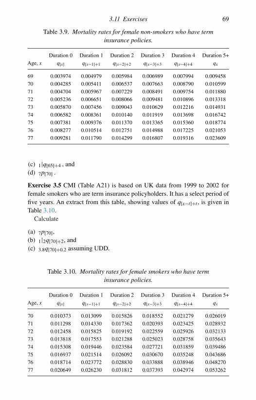
3.11 Exercises 69
Table 3.9. Mortality rates for female non-smokers who have terminsurance policies.
Age, x
Duration 0
q[x]Duration 1
q[x−1]+1
Duration 2
q[x−2]+2
Duration 3
q[x−3]+3
Duration 4
q[x−4]+4
Duration 5+
qx
69 0.003974 0.004979 0.005984 0.006989 0.007994 0.009458
70 0.004285 0.005411 0.006537 0.007663 0.008790 0.010599
71 0.004704 0.005967 0.007229 0.008491 0.009754 0.011880
72 0.005236 0.006651 0.008066 0.009481 0.010896 0.013318
73 0.005870 0.007456 0.009043 0.010629 0.012216 0.014931
74 0.006582 0.008361 0.010140 0.011919 0.013698 0.016742
75 0.007381 0.009376 0.011370 0.013365 0.015360 0.018774
76 0.008277 0.010514 0.012751 0.014988 0.017225 0.021053
77 0.009281 0.011790 0.014299 0.016807 0.019316 0.023609
(c) 1|q[65]+4 , and(d) 7p[70] .
Exercise 3.5 CMI (Table A21) is based on UK data from 1999 to 2002 forfemale smokers who are term insurance policyholders. It has a select period offive years. An extract from this table, showing values of q[x−t]+t , is given inTable 3.10.
Calculate
(a) 7p[70],(b) 1|2q[70]+2, and(c) 3.8q[70]+0.2 assuming UDD.
Table 3.10. Mortality rates for female smokers who have terminsurance policies.
Age, x
Duration 0
q[x]Duration 1
q[x−1]+1
Duration 2
q[x−2]+2
Duration 3
q[x−3]+3
Duration 4
q[x−4]+4
Duration 5+
qx
70 0.010373 0.013099 0.015826 0.018552 0.021279 0.026019
71 0.011298 0.014330 0.017362 0.020393 0.023425 0.028932
72 0.012458 0.015825 0.019192 0.022559 0.025926 0.032133
73 0.013818 0.017553 0.021288 0.025023 0.028758 0.035643
74 0.015308 0.019446 0.023584 0.027721 0.031859 0.039486
75 0.016937 0.021514 0.026092 0.030670 0.035248 0.043686
76 0.018714 0.023772 0.028830 0.033888 0.038946 0.048270
77 0.020649 0.026230 0.031812 0.037393 0.042974 0.053262

70 Life tables and selection
Exercise 3.6 A select survival model has a select period of three years.Calculate 3p53, given that
q[50] = 0.01601, 2p[50] = 0.96411,
2|q[50] = 0.02410, 2|3q[50]+1 = 0.09272.
Exercise 3.7 When posted overseas to country A at age x, the employees of alarge company are subject to a force of mortality such that, at exact duration tyears after arrival overseas (t = 0, 1, 2, 3, 4),
qA[x]+t = (6 − t)qx+t
where qx+t is on the basis of US Life Tables, 2002, Females. For those whohave lived in country A for at least five years the force of mortality at each ageis 50% greater than that of US Life Tables, 2002, Females, at the same age.Some lx values for this table are shown in Table 3.11.
Table 3.11. An extractfrom the United States
Life Tables, 2002,Females.
Age, x lx
30 98 42431 98 36232 98 29633 98 22534 98 14835 98 064· · · · · ·40 97 500
Calculate the probability that an employee posted to country A at age 30 willsurvive to age 40 if she remains in that country.
Exercise 3.8 A special survival model has a select period of three years. Func-tions for this model are denoted by an asterisk, ∗. Functions without an asteriskare taken from the Canada Life Tables 2000–02, Males. You are given that, forall values of x,
p∗[x] = 4px−5; p∗[x]+1 = 3px−1; p∗[x]+2 = 2px+2; p∗x = px+1.

3.11 Exercises 71
Table 3.12. An extractfrom the Canada Life
Tables 2000–02, Males.
Age, x lx
15 99 18016 99 13517 99 07918 99 01419 98 94220 98 86621 98 78522 98 70023 98 61524 98 52925 98 44426 98 363...
...
62 87 50363 86 45564 85 31365 84 074
A life table, tabulated at integer ages, is constructed on the basis of the specialsurvival model and the value of l∗25 is taken as 98 363 (i.e. l26 for Canada LifeTables 2000–02, Males). Some lx values for this table are shown in Table 3.12.
(a) Construct the l∗[x], l∗[x]+1, l∗[x]+2 , and l∗x+3 columns for x = 20, 21, 22.(b) Calculate 2|38q∗[21]+1, 40p∗[22], 40p∗[21]+1, 40p∗[20]+2, and 40p∗
22.
Exercise 3.9 (a) Show that a constant force of mortality between integer agesimplies that the distribution of Rx, the fractional part of the future life time,conditional on Kx = k, has the following truncated exponential distributionfor integer x, for 0 ≤ s < 1 and for k = 0, 1, . . .
Pr[Rx ≤ s | Kx = k] = 1 − exp{−µ∗x+ks}
1 − exp{−µ∗x+k}
(3.16)
where µ∗x+k = − log px+k .
(b) Show that if formula (3.16) holds for k = 0, 1, 2, . . . then the force ofmortality is constant between integer ages.
Exercise 3.10 Verify formula (3.15).
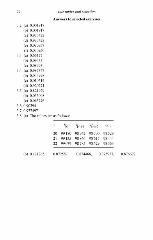
72 Life tables and selection
Answers to selected exercises
3.2 (a) 0.001917(b) 0.001917(c) 0.935422(d) 0.935423(e) 0.030957(f) 0.030950
3.3 (a) 0.66177(b) 0.09433(c) 0.08993
3.4 (a) 0.987347(b) 0.044998(c) 0.010514(d) 0.920271
3.5 (a) 0.821929(b) 0.055008(c) 0.065276
3.6 0.902943.7 0.9774973.8 (a) The values are as follows:
x l∗[x] l∗[x]+1 l∗[x]+2 lx+3
20 99 180 98 942 98 700 98 52921 99 135 98 866 98 615 98 44422 99 079 98 785 98 529 98 363
(b) 0.121265, 0.872587, 0.874466, 0.875937, 0.876692.
4
Insurance benefits
4.1 Summary
In this chapter we develop formulae for the valuation of traditional insurancebenefits. In particular, we consider whole life, term and endowment insurance.For each of these benefits we identify the random variables representing thepresent values of the benefits and we derive expressions for moments of theserandom variables. The functions we develop for traditional benefits will alsobe useful when we move to modern variable contracts.
We develop valuation functions for benefits based on the continuous futurelifetime random variable, Tx, and the curtate future lifetime random variable,Kx from Chapter 2. We introduce a new random variable, K (m)
x , which we useto value benefits which depend on the number of complete periods of length1/m years lived by a life (x). We explore relationships between the expectedpresent values of different insurance benefits.
We also introduce the actuarial notation for the expected values of the presentvalue of insurance benefits.
4.2 Introduction
In the previous two chapters, we have looked at models for future lifetime.The main reason that we need these models is to apply them to the valuationof payments which are dependent on the death or survival of a policyholderor pension plan member. Because of the dependence on death or survival, thetiming and possibly the amount of the benefit are uncertain, so the present valueof the benefit can be modelled as a random variable. In this chapter we combinesurvival models with time value of money functions to derive the distributionof the present value of an uncertain, life contingent future benefit.
We generally assume in this chapter (and in the following three chapters) thatthe interest rate is constant and fixed. This is appropriate, for example, if thepremiums for an insurance policy are invested in risk-free bonds, all yielding the
73

74 Insurance benefits
same interest rate, so that the term structure is flat. In Chapter 10 we introducemore realistic term structures, and consider some models of interest that allowfor uncertainty.
For the development of present value functions, it is generally easier, math-ematically, to work in continuous time. In the case of a death benefit, workingin continuous time means that we assume that the death payment is paid at theexact time of death. In the case of an annuity, a continuous benefit of, say, $1per year would be paid in infinitesimal units of $dt in every interval (t, t + dt).Clearly both assumptions are impractical; it will take time to process a pay-ment after death, and annuities will be paid at most weekly, not every moment(though the valuation of weekly payments is usually treated as if the paymentswere continuous, as the difference is very small). In practice, insurers and pen-sion plan actuaries work in discrete time, often with cash flow projections thatare, perhaps, monthly or quarterly. In addition, when the survival model beingused is in the form of a life table with annual increments (that is, lx for integer x),it is simplest to use annuity and insurance present value functions that assumepayments are made at integer durations only. We work in continuous time inthe first place because the mathematical development is more transparent, morecomplete and more flexible. It is then straightforward to adapt the results fromcontinuous time analysis to discrete time problems.
4.3 Assumptions
To perform calculations in this chapter, we require assumptions about mortalityand interest. We use the term basis to denote a set of assumptions used in lifeinsurance or pension calculations, and we will meet further examples of baseswhen we discuss premium calculation in Chapter 6, policy values in Chapter 7and pension liability valuation in Chapter 9.
Throughout this chapter we illustrate the results with examples using thesame survival model, which we call the Standard Ultimate Survival Model:
Makeham’s law with A = 0.00022B = 2.7 × 10⁻⁶
c = 1.124
We call this an ultimate basis to differentiate it from the standard select basisthat we will use in Chapter 6. This model is the ultimate part of the model usedin Example 3.13. We will also assume a constant rate of interest. As discussedabove, this interest assumption can be criticized as unrealistic. However, it isa convenient assumption from a pedagogical point of view, is often accurate
4.4 Valuation of insurance benefits 75
enough for practical purposes (but not always) and we relax the assumption inlater chapters.
It is also convenient to work with other interest theory functions that are incommon actuarial and financial use. We review some of these here.
We use
v = 1
1 + i
as a shorthand for discounting. The present value of a payment of S which is tobe paid in t years’ time is Svt . The force of interest per year is denoted δ where
δ = log(1 + i), 1 + i = eδ , and v = e−δ ;
δ is also known as the continuously compounded rate of interest. In financialmathematics and corporate finance contexts, and in particular if the rate of inter-est is assumed risk free, the common notation for the continuously compoundedrate of interest is r.
The nominal rate of interest compounded p times per year is denoted i(p)
where
i(p) = p((1 + i)1/p − 1
)⇔ 1 + i =
(1 + i(p)/p
)p.
The effective rate of discount per year is d where
d = 1 − v = iv = 1 − e−δ ,
and the nominal rate of discount compounded p times per year is d (p) where
d (p) = p(
1 − v1/p)
⇔ (1 − d (p)/p)p = v.
4.4 Valuation of insurance benefits
4.4.1 Whole life insurance: the continuous case, Ax
For a whole life insurance policy, the time at which the benefit will be paid isunknown until the policyholder actually dies and the policy becomes a claim.Since the present value of a future payment depends on the payment date, thepresent value of the benefit payment is a function of the time of death, and istherefore modelled as a random variable. Given a survival model and an interestrate we can derive the distribution of the present value random variable for a

76 Insurance benefits
life contingent benefit, and can therefore compute quantities such as the meanand variance of the present value.
We start by considering the value of a benefit of amount $1 payable followingthe death of a life currently aged x. Using a benefit of $1 allows us to developvaluation functions per unit of sum insured, then we can multiply these by theactual sum insured for different benefit amounts.
We first assume that the benefit is payable immediately on the death of (x).This is known as the continuous case since we work with the continuous futurelifetime random variable Tx. Although in practice there would normally bea short delay between the date of a person’s death and the time at which aninsurance company would actually pay a death benefit (due to notification ofdeath to the insurance company and legal formalities) the effect is slight andwe will ignore that delay here.
For our life (x), the present value of a benefit of $1 payable immediately ondeath is a random variable, Z , say, where
Z = vTx = e−δ Tx .
We are generally most interested in the expected value of the present valuerandom variable for some future payment. We refer to this as the ExpectedPresent Value or EPV. It is also commonly referred to as the ActuarialValue.
The EPV of the whole life insurance benefit payment with sum insured $1is E[e−δ Tx ]. In actuarial notation, we denote this expected value by Ax, wherethe bar above A denotes that the benefit is payable immediately on death.
As Tx has probability density function fx(t) = tpx µx+t , we have
Ax = E[e−δ Tx ] =∫ ∞
0e−δ t
tpx µx+tdt. (4.1)
It is worth looking at the intuition behind this formula. We use the time-lineformat that was introduced in Section 2.4 in Figure 4.1.
Consider time s, where x ≤ x + s < ω. The probability that (x) is alive attime s is spx, and the probability that (x) dies between ages x + s and x + s+ds,having survived to age x + s, is, loosely, µx+s ds, provided that ds is very small.In this case, the present value of the death benefit of $1 is e−δs.
Now we can integrate (that is, sum the infinitesimal components of) theproduct of present value and probability over all the possible death intervals s
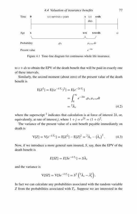
4.4 Valuation of insurance benefits 77
Time 0
x
s
x+s
s+ds
x+s+ds ω
� �
(x) survives s years
spx
� �
(x)
dies
µx+s ds
Age
Probability
Present value e−δs
Figure 4.1 Time-line diagram for continuous whole life insurance.
to s + ds to obtain the EPV of the death benefit that will be paid in exactly oneof these intervals.
Similarly, the second moment (about zero) of the present value of the deathbenefit is
E[Z2] = E[(e−δ Tx )2] = E[e−2δ Tx ]
=∫ ∞
0e−2δt
tpx µx+tdt
= 2Ax (4.2)
where the superscript 2 indicates that calculation is at force of interest 2δ, or,equivalently, at rate of interest j, where 1 + j = e2δ = (1 + i)2.
The variance of the present value of a unit benefit payable immediately ondeath is
V[Z] = V[e−δ Tx ] = E[Z2] − E[Z]2 = 2Ax − (Ax)2
. (4.3)
Now, if we introduce a more general sum insured, S, say, then the EPV of thedeath benefit is
E[SZ] = E[Se−δ Tx ] = SAx
and the variance is
V[SZ] = V[Se−δ Tx ] = S2(
2Ax − A2x
).
In fact we can calculate any probabilities associated with the random variableZ from the probabilities associated with Tx. Suppose we are interested in the

78 Insurance benefits
probability Pr[Z ≤ 0.5], for example. We can rearrange this into a probabilityfor Tx:
Pr[Z ≤ 0.5] = Pr[e−δ Tx ≤ 0.5]= Pr[−δ Tx ≤ log(0.5)]= Pr[δ Tx > − log(0.5)]= Pr[δ Tx > log(2)]= Pr[Tx > log(2)/δ]= upx
where u = log(2)/δ. We note that low values of Z are associated with highvalues of Tx. This makes sense because the benefit is more expensive to theinsurer if it is paid early, as there has been little opportunity to earn interest. Itis less expensive if it is paid later.
4.4.2 Whole life insurance: the annual case, Ax
Suppose now that the benefit of $1 is payable at the end of the year of death of(x), rather than immediately on death. To value this we use the curtate futurelifetime random variable, Kx, introduced in Chapter 2. Recall that Kx measuresthe number of complete years of future life of (x). The time to the end of theyear of death of (x) is then Kx +1. For example, if (x) lived for 25.6 years fromthe issue of the insurance policy, the observed value of Kx would be 25, and thedeath benefit payable at the end of the year of death would be payable 26 yearsfrom the policy’s issue.
We again use Z to denote the present value of the whole life insurance benefitof $1, so that Z is the random variable
Z = vKx+1.
The EPV of the benefit, E[Z], is denoted by Ax in actuarial notation.In Chapter 2 we derived the probability function for Kx, Pr[Kx = k] = k |qx,
so the EPV of the benefit is
Ax = E[vKx+1] =∞∑
k=0
vk+1k |qx = vqx + v2
1|qx + v32|qx + · · · . (4.4)
Each term on the right-hand side of this equation represents the EPV of adeath benefit of $1, payable at time k conditional on the death of (x) in (k−1, k].

4.4 Valuation of insurance benefits 79
Time 0 1 2 3
……
Amount $1 $1 $1
Discount v v2 v3
Probability qx 1|qx 2|qx
Figure 4.2 Time-line diagram for discrete whole life insurance.
In fact, we can always express the EPV of a life-contingent benefit by con-sidering each time point at which the benefit can be paid, and summing over allpossible payment times the product of
(1) the amount of the benefit,(2) the appropriate discount factor, and(3) the probability that the benefit will be paid at that time.
We will justify this more rigorously in Section 4.6. We illustrate the process forthe whole life insurance example in Figure 4.2.
The second moment of the present value is
∞∑k=0
v2(k+1)k |qx =
∞∑k=0
(v2)(k+1)k |qx = (v2)qx + (v2)2
1|qx + (v2)32|qx + · · · .
Just as in the continuous case, we can calculate the second moment about zeroof the present value by an adjustment in the rate of interest from i to (1+ i)2 −1.We define
2Ax =∞∑
k=0
v2(k+1)k |qx , (4.5)
and so the variance of the present value of a benefit of S payable at the end ofthe year of death is
S2(
2Ax − (Ax)2)
. (4.6)
4.4.3 Whole life insurance: the 1/mthly case, A(m)x
In Chapter 2 we introduced the random variable Kx, representing the curtatefuture lifetime of (x), and we saw in Section 4.4.2 that the present value of an

80 Insurance benefits
insurance benefit payable at the end of the year of death can be expressed interms of Kx.
We now define the random variable K (m)x , where m > 1 is an integer, to
be the future lifetime of (x) in years rounded to the lower 1m th of a year. The
most common values of m are 2, 4 and 12, corresponding to half years, quarteryears and months. Thus, for example, K (4)
x represents the future lifetime of (x),rounded down to the lower 1/4.
Symbolically, if we let � denote the integer part (or floor) function, then
K (m)x = 1
m�mTx . (4.7)
For example, suppose (x) lives exactly 23.675 years. ThenKx = 23, K (2)
x = 23.5, K (4)x = 23.5, and K (12)
x = 23 812 = 23.6667.
Note that K (m)x is a discrete random variable. K (m)
x = k indicates that the life(x) dies in the interval [k, k + 1/m), for (k = 0, 1
m , 2m , . . .).
The probability function for K (m)x can be derived from the associated
probabilities for Tx. For k = 0, 1m , 2
m , . . . ,
Pr[K (m)x = k] = Pr
[k ≤ Tx < k + 1
m
]= k | 1
mqx = kpx − k+ 1
mpx .
In Figure 4.3 we show the time-line for the mthly benefit. At the end of each1/m year period, we show the amount of benefit due, conditional on the deathof the insured life in the previous 1/m year interval, the probability that theinsured life dies in the relevant interval, and the appropriate discount factor.
Suppose, for example, that m = 12. A whole life insurance benefit payableat the end of the month of death has present value random variable Z where
Z = vK (12)x +1/12.
Time 0 1/m 2/m 3/m
……
Amount $1 $1 $1
Discount v1/m v2/m v3/m
Probability 1m
qx 1m
| 1m
qx 2m
| 1m
qx
Figure 4.3 Time-line diagram for mthly whole life insurance.

4.4 Valuation of insurance benefits 81
We let A(12)x denote the EPV of this benefit, so that
E[Z] = A(12)x = v1/12
112
qx + v2/12112
| 112
qx + v3/122
12| 1
12qx + v4/12
312
| 112
qx
+ · · · .
Similarly, for any m,
A(m)x = v1/m
1m
qx + v2/m1m| 1
mqx + v3/m
2m| 1
mqx + v4/m
3m| 1
mqx + · · · (4.8)
=∞∑
k=0
vk+1
m km| 1
mqx. (4.9)
As for the continuous and annual cases, we can derive the variance of the presentvalue of the mthly whole life benefit by adjusting the interest rate for the firstterm in the variance. We have
E[Z2] = E[v2(K (12)x +1/12)] = E[(v2)K (12)
x +1/12] = 2A(12)x ,
so the variance is
2A(12)x − (A(12)
x )2.
4.4.4 Recursions
In practice, it would be very unusual for an insurance policy to provide thedeath benefit at the end of the year of death. Nevertheless, the annual insurancefunction Ax is still useful. We are often required to work with annual life tables,such as those in Chapter 3, in which case we would start by calculating theannual function Ax, then adjust for a more appropriate frequency using therelationships and assumptions we develop later in this chapter.
Using the annual life table in a spreadsheet, we can calculate the values ofAx using backwards recursion. To do this, we start from the highest age in thetable, ω. We assume all lives expire by age ω, so that qω−1 = 1. If the life tabledoes not have a limiting age, we choose a suitably high value for ω so that qω−1
is as close to 1 as we like. This means that any life attaining age ω − 1 may betreated as certain to die before age ω, in which case we know that Kω−1 = 0and so
Aω−1 = E[vKω−1+1] = v.
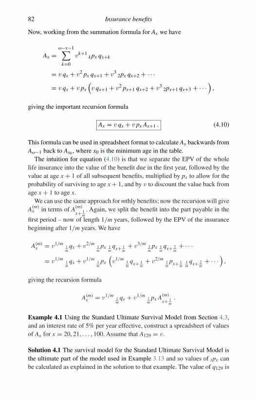
82 Insurance benefits
Now, working from the summation formula for Ax we have
Ax =ω−x−1∑
k=0
vk+1kpx qx+k
= v qx + v2 px qx+1 + v32px qx+2 + · · ·
= v qx + v px
(v qx+1 + v2 px+1 qx+2 + v3
2px+1 qx+3 + · · ·)
,
giving the important recursion formula
Ax = v qx + v px Ax+1 . (4.10)
This formula can be used in spreadsheet format to calculate Ax backwards fromAω−1 back to Ax0 , where x0 is the minimum age in the table.
The intuition for equation (4.10) is that we separate the EPV of the wholelife insurance into the value of the benefit due in the first year, followed by thevalue at age x + 1 of all subsequent benefits, multiplied by px to allow for theprobability of surviving to age x + 1, and by v to discount the value back fromage x + 1 to age x.
We can use the same approach for mthly benefits; now the recursion will giveA(m)
x in terms of A(m)
x+ 1m
. Again, we split the benefit into the part payable in the
first period – now of length 1/m years, followed by the EPV of the insurancebeginning after 1/m years. We have
A(m)x = v1/m
1m
qx + v2/m1m
px 1m
qx+ 1m
+ v3/m2m
px 1m
qx+ 2m
+ · · ·
= v1/m1m
qx + v1/m1m
px
(v1/m
1m
qx+ 1m
+ v2/m1m
px+ 1m
1m
qx+ 2m
+ · · ·)
,
giving the recursion formula
A(m)x = v1/m
1m
qx + v1/m1m
px A(m)
x+ 1m
.
Example 4.1 Using the Standard Ultimate Survival Model from Section 4.3,and an interest rate of 5% per year effective, construct a spreadsheet of valuesof Ax for x = 20, 21, . . . , 100. Assume that A129 = v.
Solution 4.1 The survival model for the Standard Ultimate Survival Model isthe ultimate part of the model used in Example 3.13 and so values of tpx canbe calculated as explained in the solution to that example. The value of q129 is

4.4 Valuation of insurance benefits 83
Table 4.1. Spreadsheet results for Example 4.1, for the calculationof Ax using the Standard Ultimate Survival Model.
x Ax x Ax x Ax
20 0.04922 47 0.16577 74 0.4921521 0.05144 48 0.17330 75 0.5086822 0.05378 49 0.18114 76 0.5253623 0.05622 50 0.18931 77 0.5421724 0.05879 51 0.19780 78 0.5590625 0.06147 52 0.20664 79 0.5759926 0.06429 53 0.21582 80 0.5929327 0.06725 54 0.22535 81 0.6098428 0.07034 55 0.23524 82 0.6266629 0.07359 56 0.24550 83 0.6433630 0.07698 57 0.25613 84 0.6599031 0.08054 58 0.26714 85 0.6762232 0.08427 59 0.27852 86 0.6922933 0.08817 60 0.29028 87 0.7080634 0.09226 61 0.30243 88 0.7234935 0.09653 62 0.31495 89 0.7385336 0.10101 63 0.32785 90 0.7531737 0.10569 64 0.34113 91 0.7673538 0.11059 65 0.35477 92 0.7810439 0.11571 66 0.36878 93 0.7942340 0.12106 67 0.38313 94 0.8068841 0.12665 68 0.39783 95 0.8189742 0.13249 69 0.41285 96 0.8304943 0.13859 70 0.42818 97 0.8414344 0.14496 71 0.44379 98 0.8517745 0.15161 72 0.45968 99 0.8615346 0.15854 73 0.47580 100 0.87068
0.99996, which is indeed close to 1. We can use the formula
Ax = vqx + vpxAx+1
to calculate recursively A128, A127, . . . , A20, starting from A129 = v. Values forx = 20, 21, . . . , 100, are given in Table 4.1. �
Example 4.2 Using the Standard Ultimate Survival Model from Section 4.3,and an interest rate of 5% per year effective, develop a spreadsheet of valuesof A(12)
x for x starting at age 20, in steps of 1/12.
Solution 4.2 For this example, we follow exactly the same process as for theprevious example, except that we let the ages increase by 1/12 year in each
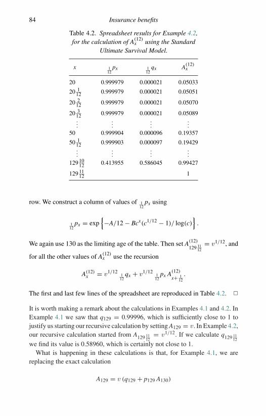
84 Insurance benefits
Table 4.2. Spreadsheet results for Example 4.2,for the calculation of A(12)
x using the StandardUltimate Survival Model.
x 112
px 112
qx A(12)x
20 0.999979 0.000021 0.05033
20 112 0.999979 0.000021 0.05051
20 212 0.999979 0.000021 0.05070
20 312 0.999979 0.000021 0.05089...
......
...50 0.999904 0.000096 0.19357
50 112 0.999903 0.000097 0.19429...
......
...129 10
12 0.413955 0.586045 0.99427
129 1112 1
row. We construct a column of values of 112
px using
112
px = exp{−A/12 − Bcx(c1/12 − 1)/ log(c)
}.
We again use 130 as the limiting age of the table. Then set A(12)
129 1112
= v1/12, and
for all the other values of A(12)x use the recursion
A(12)x = v1/12
112
qx + v1/12112
px A(12)
x+ 112
.
The first and last few lines of the spreadsheet are reproduced in Table 4.2. �
It is worth making a remark about the calculations in Examples 4.1 and 4.2. InExample 4.1 we saw that q129 = 0.99996, which is sufficiently close to 1 tojustify us starting our recursive calculation by setting A129 = v. In Example 4.2,our recursive calculation started from A129 11
12= v1/12. If we calculate q129 11
12we find its value is 0.58960, which is certainly not close to 1.
What is happening in these calculations is that, for Example 4.1, we arereplacing the exact calculation
A129 = v (q129 + p129 A130)
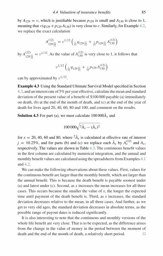
4.4 Valuation of insurance benefits 85
by A129 = v, which is justifiable because p129 is small and A130 is close to 1,meaning that v(q129 + p129 A130) is very close to v. Similarly, for Example 4.2,we replace the exact calculation
A(12)
129 1112
= v1/12(
112
q129 1112
+ 112
p129 1112
A(12)130
)
by A(12)
129 1112
= v1/12. As the value of A(12)130 is very close to 1, it follows that
v1/12(
112
q129 1112
+ 112
p129 A(12)130
)
can by approximated by v1/12.
Example 4.3 Using the Standard Ultimate Survival Model specified in Section4.3, and an interest rate of 5% per year effective, calculate the mean and standarddeviation of the present value of a benefit of $100 000 payable (a) immediatelyon death, (b) at the end of the month of death, and (c) at the end of the year ofdeath for lives aged 20, 40, 60, 80 and 100, and comment on the results.
Solution 4.3 For part (a), we must calculate 100 000Ax and
100 000√
2Ax − (Ax)2
for x = 20, 40, 60 and 80, where 2Ax is calculated at effective rate of interestj = 10.25%, and for parts (b) and (c) we replace each Ax by A(12)
x and Ax,respectively. The values are shown in Table 4.3. The continuous benefit valuesin the first column are calculated by numerical integration, and the annual andmonthly benefit values are calculated using the spreadsheets from Examples 4.1and 4.2.
We can make the following observations about these values. First, values forthe continuous benefit are larger than the monthly benefit, which are larger thanthe annual benefit. This is because the death benefit is payable soonest under(a) and latest under (c). Second, as x increases the mean increases for all threecases. This occurs because the smaller the value of x, the longer the expectedtime until payment of the death benefit is. Third, as x increases, the standarddeviation decreases relative to the mean, in all three cases. And further, as weget to very old ages, the standard deviation decreases in absolute terms, as thepossible range of payout dates is reduced significantly.
It is also interesting to note that the continuous and monthly versions of thewhole life benefit are very close. That is to be expected, as the difference arisesfrom the change in the value of money in the period between the moment ofdeath and the end of the month of death, a relatively short period. �
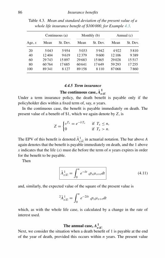
86 Insurance benefits
Table 4.3. Mean and standard deviation of the present value of awhole life insurance benefit of $100 000, for Example 4.3.
Continuous (a) Monthly (b) Annual (c)
Age, x Mean St. Dev. Mean St. Dev. Mean St. Dev.
20 5 043 5 954 5 033 5 942 4 922 5 81040 12 404 9 619 12 379 9 600 12 106 9 38960 29 743 15 897 29 683 15 865 29 028 15 51780 60 764 17 685 60 641 17 649 59 293 17 255
100 89 341 8 127 89 158 8 110 87 068 7 860
4.4.5 Term insurance
The continuous case, A1x:n
Under a term insurance policy, the death benefit is payable only if thepolicyholder dies within a fixed term of, say, n years.
In the continuous case, the benefit is payable immediately on death. Thepresent value of a benefit of $1, which we again denote by Z , is
Z ={vTx = e−δ Tx if Tx ≤ n,0 if Tx > n.
The EPV of this benefit is denoted A 1x:n in actuarial notation. The bar above A
again denotes that the benefit is payable immediately on death, and the 1 abovex indicates that the life (x) must die before the term of n years expires in orderfor the benefit to be payable.
Then
A 1x:n =
∫ n
0e−δt
tpxµx+tdt (4.11)
and, similarly, the expected value of the square of the present value is
2A 1x:n =
∫ n
0e−2δt
tpxµx+tdt
which, as with the whole life case, is calculated by a change in the rate ofinterest used.
The annual case, A 1x:n
Next, we consider the situation when a death benefit of 1 is payable at the endof the year of death, provided this occurs within n years. The present value

4.4 Valuation of insurance benefits 87
random variable for the benefit is now
Z ={vKx+1 if Kx ≤ n − 1,0 if Kx ≥ n.
The EPV of the benefit is denoted A 1x:n so that
A 1x:n =
n−1∑k=0
vk+1k |qx. (4.12)
The 1/mthly case, A(m)1
x:nWe now consider the situation when a death benefit of 1 is payable at the end ofthe 1/mth year of death, provided this occurs within n years. The present valuerandom variable for the benefit is
Z ={
vK (m)x + 1
m if K (m)x ≤ n − 1
m ,
0 if K (m)x ≥ n.
The EPV of the benefit is denoted A(m)1
x:n so that
A(m)1
x:n =mn−1∑k=0
v(k+1)/mkm| 1
mqx . (4.13)
Example 4.4 Using the Standard Ultimate Survival Model as specified in
Section 4.3, with interest at 5% per year effective, calculate A 1x:10
, A(4)1
x:10and A 1
x:10for x = 20, 40, 60 and 80 and comment on the values.
Solution 4.4 We use formula (4.11) with n = 10 to calculate A 1x:10
(using
numerical integration), and formulae (4.13) and (4.12), with m = 4 and n = 10
to calculate A(4)1
x:10and A1
x:10.
The values are shown in Table 4.4, and we observe that values in each caseincrease as x increases, reflecting the fact that the probability of death in a 10-year period increases with age for the survival model we are using. The orderingof values at each age is the same as in Example 4.3, for the same reason – theordering reflects the fact that any payment under the continuous benefit will bepaid earlier than a payment under the quarterly benefit. The end year benefit ispaid later than the quarterly benefit, except when the death occurs in the finalquarter of the year, in which case the benefit is paid at the same time. �

88 Insurance benefits
Table 4.4. EPVs of term insurance benefits.
x A 1x:10
A(4)1
x:10A 1
x:10
20 0.00214 0.00213 0.0020940 0.00587 0.00584 0.0057360 0.04356 0.04329 0.0425280 0.34550 0.34341 0.33722
4.4.6 Pure endowment
Pure endowment benefits are conditional on the survival of the policyholder. Forexample, a 10-year pure endowment with sum insured $10 000, issued to (x),will pay $10 000 in 10 years if (x) is still alive at that time, and will pay nothing if(x) dies before age x +10. Pure endowment benefits are not sold as stand-alonepolicies, but may be sold in conjunction with term insurance benefits to createthe endowment insurance benefit described in the following section. However,pure endowment valuation functions turn out to be very useful.
The pure endowment benefit of $1, issued to a life aged x, with a term of nyears has present value Z , say, where:
Z ={
0 if Tx < n,vn if Tx ≥ n.
There are two ways to denote the EPV of the pure endowment benefit usingactuarial notation. It may be denoted A 1
x:n . The ‘1’ over the term subscriptindicates that the term must expire before the life does for the benefit to bepaid. This notation is consistent with the term insurance notation, but it canbe cumbersome, considering that this is a function which is used very oftenin actuarial calculations. A more convenient standard actuarial notation for theEPV of the pure endowment is nEx.
If we rewrite the definition of Z above, we have
Z ={
0 with probability 1 − npx ,vn with probability npx .
(4.14)
Then we can see that the EPV is
A 1x:n = vn
npx . (4.15)
Note that because the pure endowment will be paid only at time n, assuming thelife survives, there is no need to specify continuous and discrete time versions;there is only a discrete time version.

4.4 Valuation of insurance benefits 89
We will generally use the more direct notation vnnpx or nEx for the pure
endowment function, rather than the A 1x:n notation.
4.4.7 Endowment insurance
An endowment insurance provides a combination of a term insurance and apure endowment. The sum insured is payable on the death of (x) should (x) diewithin a fixed term, say n years, but if (x) survives for n years, the sum insuredis payable at the end of the nth year.
Traditional endowment insurance policies were popular in Australia, NorthAmerica and the UK up to the 1990s, but are rarely sold these days in thesemarkets. However, as with the pure endowment, the valuation function turnsout to be quite useful in other contexts. Also, companies operating in theseterritories will be managing the ongoing liabilities under the policies alreadywritten for some time to come. Furthermore, traditional endowment insuranceis still relevant and popular in some other insurance markets.
We first consider the case when the death benefit (of amount 1) is payableimmediately on death. The present value of the benefit is Z , say, where
Z ={vTx = e−δTx if Tx < n,vn if Tx ≥ n
= vmin(Tx ,n) = e−δ min(Tx ,n).
Thus, the EPV of the benefit is
E[Z] =∫ n
0e−δt
tpxµx+tdt +∫ ∞
ne−δn
tpxµx+tdt
=∫ n
0e−δt
tpxµx+tdt + e−δnnpx
= A 1x:n + A 1
x:n
and in actuarial notation we write
Ax:n = A1x:n + A 1
x:n . (4.16)
Similarly, the expected value of the squared present value of the benefit is∫ n
0e−2δt
tpxµx+tdt + e−2δnnpx
which we denote 2Ax:n .
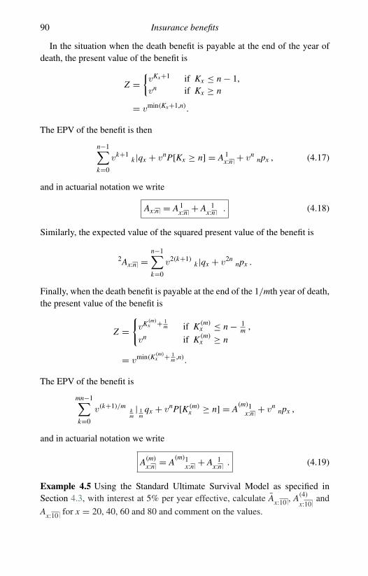
90 Insurance benefits
In the situation when the death benefit is payable at the end of the year ofdeath, the present value of the benefit is
Z ={vKx+1 if Kx ≤ n − 1,vn if Kx ≥ n
= vmin(Kx+1,n).
The EPV of the benefit is then
n−1∑k=0
vk+1k |qx + vnP[Kx ≥ n] = A 1
x:n + vnnpx , (4.17)
and in actuarial notation we write
Ax:n = A 1x:n + A 1
x:n . (4.18)
Similarly, the expected value of the squared present value of the benefit is
2Ax:n =n−1∑k=0
v2(k+1)k |qx + v2n
npx .
Finally, when the death benefit is payable at the end of the 1/mth year of death,the present value of the benefit is
Z ={
vK (m)x + 1
m if K (m)x ≤ n − 1
m ,
vn if K (m)x ≥ n
= vmin(K (m)x + 1
m ,n).
The EPV of the benefit is
mn−1∑k=0
v(k+1)/mkm| 1
mqx + vnP[K (m)
x ≥ n] = A(m)1
x:n + vnnpx ,
and in actuarial notation we write
A(m)
x:n = A(m)1
x:n + A 1x:n . (4.19)
Example 4.5 Using the Standard Ultimate Survival Model as specified inSection 4.3, with interest at 5% per year effective, calculate Ax:10 , A(4)
x:10and
Ax:10 for x = 20, 40, 60 and 80 and comment on the values.
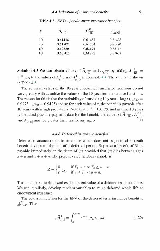
4.4 Valuation of insurance benefits 91
Table 4.5. EPVs of endowment insurance benefits.
x Ax:10 A(4)
x:10Ax:10
20 0.61438 0.61437 0.6143340 0.61508 0.61504 0.6149460 0.62220 0.62194 0.6211680 0.68502 0.68292 0.67674
Solution 4.5 We can obtain values of Ax:10 and Ax:10 by adding A 1x:10
=v10
10px to the values of A 1x:10
and A 1x:10
in Example 4.4. The values are shown
in Table 4.5.The actuarial values of the 10-year endowment insurance functions do not
vary greatly with x, unlike the values of the 10-year term insurance functions.The reason for this is that the probability of surviving 10 years is large (10p20 =0.9973, 10p60 = 0.9425) and so for each value of x, the benefit is payable after10 years with a high probability. Note that v10 = 0.6139, and as time 10 yearsis the latest possible payment date for the benefit, the values of Ax:10 , A(4)
x:10and Ax:10 must be greater than this for any age x. �
4.4.8 Deferred insurance benefits
Deferred insurance refers to insurance which does not begin to offer deathbenefit cover until the end of a deferred period. Suppose a benefit of $1 ispayable immediately on the death of (x) provided that (x) dies between agesx + u and x + u + n. The present value random variable is
Z ={
0 if Tx < u or Tx ≥ u + n,e−δTx if u ≤ Tx < u + n.
This random variable describes the present value of a deferred term insurance.We can, similarly, develop random variables to value deferred whole life orendowment insurance.
The actuarial notation for the EPV of the deferred term insurance benefit is
u|A 1x:n . Thus
u|A 1x:n =
∫ u+n
ue−δt
tpxµx+tdt. (4.20)

92 Insurance benefits
Changing the integration variable to s = t − u gives
u|A 1x:n =
∫ n
0e−δ(s+u)
s+upx µx+s+u ds
= e−δuupx
∫ n
0e−δs
spx+u µx+s+u ds
= e−δuupx A 1
x+u:n = vuupx A 1
x+u:n = uEx A 1x+u:n . (4.21)
A further expression for u|A 1x:n is
u|A 1x:n = A 1
x:u+n− A 1
x:u (4.22)
which follows from formula (4.20) since
∫ u+n
ue−δt
tpxµx+tdt =∫ u+n
0e−δt
tpxµx+tdt −∫ u
0e−δt
tpxµx+tdt.
Thus, the EPV of a deferred term insurance benefit can be found by differencingthe EPVs of term insurance benefits for terms u + n and u.
Note the role of the pure endowment term uEx = vuupx in equation (4.21).
This acts similarly to a discount function. If the life survives u years, to the endof the deferred period, then the EPV at that time of the term insurance is A 1
x+u:n .Multiplying by vu
upx converts this to the EPV at the start of the deferred period.Our main interest in this EPV is as a building block. We observe, for example,
that an n-year term insurance can be decomposed as the sum of n deferred terminsurance policies, each with a term of one year, and we can write
A 1x:n =
∫ n
0e−δt
tpxµx+tdt
=n−1∑r=0
∫ r+1
re−δt
tpxµx+tdt
=n−1∑r=0
r|A 1x:1
. (4.23)
A similar decomposition applies to a whole life insurance policy and we canwrite
Ax =∞∑
r=0
r|A 1x:1
.
4.5 Relating Ax , Ax and A(m)x 93
We can derive similar results for the deferred benefit payable at the end of theyear of death, with EPV denoted u|A 1
x:n .In particular, it is useful to note that
Ax = A 1x:n + n|Ax (4.24)
so that
A 1x:n = Ax − n|Ax
= Ax − vnnpx Ax+n .
This relationship can be used to calculate A 1x:n for integer x and n given a table
of values of Ax and lx.
4.5 Relating Ax , Ax and A(m)x
We mentioned in the introduction to this chapter that, even though insurancecontracts with death benefits payable at the end of the year of death are veryunusual, functions like Ax are still useful. The reason for this is that we canapproximate Ax or A(m)
x from Ax, and we might wish to do this if the onlyinformation we had was a life table, with integer age functions only, rather thana formula for the force of mortality that could be applied for all ages.
In Table 4.6 we show values of the ratios of A(4)x to Ax and Ax to Ax, using
the Standard Ultimate Survival Model from Section 4.3, with interest at 5% peryear effective.
We see from Table 4.6 that, over a very wide range of ages, the ratios ofA(4)
x to Ax and Ax to Ax are remarkably stable, giving the appearance of beingindependent of x. In the following section we show how we can approximatevalues of A(m)
x to Ax using values of Ax.
4.5.1 Using the uniform distribution of deaths assumption
The difference between Ax and Ax depends on the lifetime distribution betweenages y and y + 1 for all y ≥ x. If we do not have information about this,for example, because we have mortality information only at integer ages, wecan approximate the relationship between the continuous function Ax and thediscrete function Ax using the fractional age assumptions that we introduced inSection 3.3. The most convenient fractional age assumption for this purpose isthe uniform distribution of deaths assumption, or UDD.
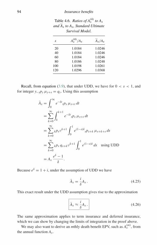
94 Insurance benefits
Table 4.6. Ratios of A(4)x to Ax
and Ax to Ax, Standard UltimateSurvival Model.
x A(4)x /Ax Ax/Ax
20 1.0184 1.024640 1.0184 1.024660 1.0184 1.024680 1.0186 1.0248
100 1.0198 1.0261120 1.0296 1.0368
Recall, from equation (3.9), that under UDD, we have for 0 < s < 1, andfor integer y, spy µy+s = qy. Using this assumption
Ax =∫ ∞
0e−δt
tpx µx+t dt
=∞∑
k=0
∫ k+1
ke−δt
tpx µx+t dt
=∞∑
k=0
kpxvk+1∫ 1
0e(1−s)δ
spx+k µx+k+s ds
=∞∑
k=0
kpx qx+kvk+1∫ 1
0e(1−s)δ ds using UDD
= Axeδ − 1
δ.
Because eδ = 1 + i, under the assumption of UDD we have
Ax = i
δAx . (4.25)
This exact result under the UDD assumption gives rise to the approximation
Ax ≈ i
δAx . (4.26)
The same approximation applies to term insurance and deferred insurance,which we can show by changing the limits of integration in the proof above.
We may also want to derive an mthly death benefit EPV, such as A(m)x , from
the annual function Ax.

4.5 Relating Ax , Ax and A(m)x 95
Under the UDD assumption we find that
A(m)x = i
i(m)Ax , (4.27)
and the right-hand side is used as an approximation to A(m)x . The proof of formula
(4.27) is left as an exercise for the reader.We stress that these approximations apply only to death benefits. The endow-
ment insurance combines the death and survival benefits, so we need to splitoff the death benefit before applying one of the approximations. That is, underthe UDD approach
Ax:n ≈ iδA 1
x:n + vnnpx . (4.28)
4.5.2 Using the claims acceleration approach
The claims acceleration approach is a more heuristic way of deriving an approx-imate relationship between the annual death benefit EPV, Ax, and the mthly orcontinuous EPVs, A(m)
x and Ax. The only difference between these benefits isthe timing of the payment. Consider, for example, Ax and A(4)
x . Since the insuredlife (x) dies in the year of age x + Kx to x + Kx + 1, under the end year of deathbenefit (valued by Ax), the sum insured is paid at time Kx + 1. Under the end ofquarter-year of death benefit (valued by A(4)
x ), the benefit will be paid either atKx +1/4, Kx +2/4, Kx +3/4 or Kx +1 depending on the quarter year in whichthe death occurred. If the deaths occur evenly over the year (the same assump-tion as we use in the UDD approach), then, on average, the benefit is paid attime Kx + 5/8, which is 3/8 years earlier than the end of year of death benefit.
Similarly, suppose the benefit is paid at the end of the month of death.Assum-ing deaths occur uniformly over the year, then on average the benefit is paid atKx + 13/24, which is 11/24 years earlier than the end year of death benefit.
In general, for an mthly death benefit, assuming deaths are uniformly dis-tributed over the year of age, the average time of payment of the death benefitis (m + 1)/2m in the year of death.
So we have the resulting approximation
A(m)x ≈ qxv
m+12m + 1|qx v1+ m+1
2m + 2|qx v2+ m+12m + · · ·
=∞∑
k=0
k |qxvk+ m+1
2m
= (1 + i)m−12m
∞∑k=0
k |qxvk+1.

96 Insurance benefits
That is
A(m)x ≈ (1 + i)
m−12m Ax . (4.29)
For the continuous benefit EPV, Ax, we let m → ∞ in equation (4.29), to givethe approximation
Ax ≈ (1 + i)1/2Ax . (4.30)
This is explained by the fact that, if the benefit is paid immediately on death,and lives die uniformly through the year, then, on average, the benefit is paidhalf-way through the year of death, which is half a year earlier than the benefitvalued by Ax.
As with the UDD approach, these approximations apply only to death bene-fits. Hence, for an endowment insurance using the claims acceleration approachwe have
Ax:n ≈ (1 + i)1/2A 1x:n + vn
npx . (4.31)
Note that both the UDD and the claims acceleration approaches give valuesfor A(m)
x or Ax such that the ratios A(m)x /Ax = i/i(m) and Ax/Ax = i/δ are
independent of x. Note also that for i = 5%, i/i(4) = 1.0186 and i/δ = 1.0248,whilst (1 + i)3/8 = 1.0185 and (1 + i)1/2 = 1.0247. The values in Table 4.6show that both approaches give good approximations in these cases.
4.6 Variable insurance benefits
For all the insurance benefits studied in this chapter the EPV of the benefit canbe expressed as the sum over all the possible payment dates of the product ofthree terms:
• the amount of benefit paid,• the appropriate discount factor for the payment date, and• the probability that the benefit will be paid at that payment date.
This approach works for the EPV of any traditional benefit – that is, wherethe future lifetime is the sole source of uncertainty. It will not generate highermoments or probability distributions.
The approach can be justified technically using indicator random variables.Consider a life contingent event E – for example, E is the event that a life aged

4.6 Variable insurance benefits 97
x dies in the interval (k, k + 1]. The indicator random variable is
I(E) ={
1 if E is true,0 if E is false.
In this example, Pr[E is True ] = k |qx, so the expected value of the indicatorrandom variable is
E[I(E)] = 1(k |qx) + 0(1 − k |qx) = k |qx ,
and, in general, the expected value of an indicator random variable is theprobability of the indicator event.
Consider, for example, an insurance that pays $1 000 after 10 years if (x) hasdied by that time, and $2 000 after 20 years if (x) dies in the second 10-yearperiod, with no benefit otherwise.
We can write the present value random variable as
1 000 I(Tx ≤ 10)v10 + 2 000 I(10 < Tx ≤ 20)v20
and the EPV is then
1 000 10qx v10 + 2 000 10|10qx v20.
Indicator random variables can also be used for continuous benefits. Here weconsider indicators of the form
I(t < Tx ≤ t + dt)
for infinitesimal dt, with associated probability
E[I(t < Tx ≤ t + dt)] = Pr[t < Tx ≤ t + dt]= Pr[Tx > t] Pr[Tx < t + dt|Tx > t]≈ tpx µx+t dt.
Consider, for example, an increasing insurance policy with a death benefit ofTx payable at the moment of death. That is, the benefit is exactly equal to thenumber of years lived by an insured life from age x to his or her death. This is acontinuous whole life insurance under which the benefit is a linearly increasingfunction.
To find the EPV of this benefit, we note that the payment may be made atany time, so we consider all the infinitesimal intervals (t, t + dt), and we sumover all these intervals by integrating from t = 0 to t = ∞.
98 Insurance benefits
First, we identify the amount, discount factor and probability for a benefitpayable in the interval (t, t + dt). The amount is t, the discount factor is e−δt .The probability that the benefit is paid in the interval (t, t +dt) is the probabilitythat the life survives from x to x + t, and then dies in the infinitesimal interval(t, t + dt), which gives an approximate probability of tpx µx+t dt.
So, we can write the EPV of this benefit as∫ ∞
0t e−δt
tpx µx+tdt. (4.32)
In actuarial notation we write this as (I A)x. The I here stands for ‘increasing’and the bar over the I denotes that the increases are continuous.
An alternative approach to deriving equation (4.32) is to identify the presentvalue random variable for the benefit, denoted by Z , say, in terms of the futurelifetime random variable,
Z = Tx e−δTx .
Then any moment of Z can be found from
E[Zk ] =∫ ∞
0
(t e−δt)k
tpx µx+t dt .
The advantage of the first approach is that it is very flexible and generally quick,even for very complex benefits.
If the policy term ceases after a fixed term of n years, the EPV of the deathbenefit is
(I A) 1x:n =
∫ n
0t e−δt
tpx µx+tdt.
There are a number of other increasing or decreasing benefit patterns that arefairly common. We present several in the following examples.
Example 4.6 Consider an n-year term insurance policy issued to (x) underwhich the death benefit is k +1 if death occurs between ages x+k and x+k +1,for k = 0, 1, 2, . . . , n − 1.
(a) Derive a formula for the EPV of the benefit using the first approachdescribed, that is multiplying together the amount, the discount factor andthe probability of payment, and summing for each possible payment date.
(b) Derive a formula for the variance of the present value of the benefit.
Solution 4.6 (a) Suppose that the benefit is payable at time k + 1, for k =0, 1, . . . , n − 1. Then if the benefit is paid at time k + 1, the benefit amount

4.6 Variable insurance benefits 99
is $(k + 1). The discount factor is vk+1 and the probability that the benefitis paid at that date is the probability that the policyholder died in the year(k, k + 1], which is k |qx, so the EPV of the death benefit is
n−1∑k=0
vk+1(k + 1) k |qx .
In actuarial notation the above EPV is denoted (IA) 1x:n .
If the term n is infinite, so that this is a whole life version of the increasingannual policy, with benefit k + 1 following death in the year k to k + 1, theEPV of the death benefit is denoted (IA)x where
(IA)x =∞∑
k=0
vk+1(k + 1) k |qx .
(b) We must go back to first principles. First, we identify the random variable as
Z ={(Kx + 1)vKx+1 if Kx ≤ n,0 if Kx > n.
So
E[Z2] =n−1∑k=0
v2(k+1)(k + 1)2k |qx ,
and the variance is
V[Z] =n−1∑k=0
v2(k+1)(k + 1)2k |qx −
((IA) 1
x:n
)2.
�
Example 4.7 A whole life insurance policy offers an increasing death benefitpayable at the end of the quarter year of death. If (x) dies in the first year of thecontract, then the benefit is 1, in the second year it is 2, and so on. Derive anexpression for the EPV of the death benefit.
Solution 4.7 First, we note that the possible payment dates are 1/4, 2/4, 3/4, … .Next, if (x) dies in the first year, then the benefit payable is 1, if death occursin the second year the benefit payable is 2, and so on. Third, corresponding tothe possible payment dates, the discount factors are v1/4, v2/4, . . . .
The probabilities associated with the payment dates are 14qx, 1
4| 1
4qx, 2
4| 1
4qx,
34| 1
4qx, . . . .
100 Insurance benefits
Hence, the EPV, which is denoted (IA(4))x, can be calculated as
14qx v
14 + 1
4| 1
4qx v
24 + 2
4| 1
4qx v
34 + 3
4| 1
4qx v1
+ 2(
1| 14qx v1 1
4 + 1 14| 1
4qx v1 2
4 + 1 24| 1
4qx v1 3
4 + 1 34| 1
4qx v2
)+ 3
(2| 1
4qx v2 1
4 + 2 14| 1
4qx v2 2
4 + 2 24| 1
4qx v2 3
4 + 2 34| 1
4qx v3
)+ · · ·
= A(4)1
x:1+ 2 1|A(4)1
x:1+ 3 2|A(4)1
x:1+ · · · .
�
We now consider the case when the amount of the death benefit increasesin geometric progression. This is important in practice because compoundreversionary bonuses will increase the sum insured as a geometric progression.
Example 4.8 Consider an n-year term insurance issued to (x) under which thedeath benefit is paid at the end of the year of death. The benefit is 1 if deathoccurs between ages x and x + 1, 1 + j if death occurs between ages x + 1 andx + 2, (1 + j)2 if death occurs between ages x + 2 and x + 3, and so on. Thus,if death occurs between ages x + k and x + k + 1, the death benefit is (1 + j)k
for k = 0, 1, 2, . . . , n − 1. Derive a formula for the EPV of this death benefit.
Solution 4.8 The amount of benefit is 1 if the benefit is paid at time 1, (1 + j)if the benefit is paid at time 2, (1 + j)2 if the benefit is paid at time 3, and soon, up to time n. The EPV of the death benefit is then
v qx + (1 + j)v21|qx + (1 + j)2 v3
2|qx + · · · + (1 + j)n−1 vnn−1|qx
=n−1∑k=0
vk+1(1 + j)kk |qx
= 1
1 + j
n−1∑k=0
vk+1(1 + j)k+1k |qx
= A 1x:n i∗ (4.33)
where
i∗ = 1 + i
1 + j− 1 = i − j
1 + j.
�
The notation A 1x:n i∗ indicates that the EPV is calculated using the rate of interest
i∗, rather than i. In most practical situations, i > j so that i∗ > 0.
4.8 Notes and further reading 101
Example 4.9 Consider an insurance policy issued to (x) under which the deathbenefit is (1 + j)t if death occurs at age x + t, with the death benefit beingpayable immediately on death.
(a) Derive an expression for the EPV of the death benefit if the policy is ann-year term insurance.
(b) Derive an expression for the EPV of the death benefit if the policy is awhole life insurance.
Solution 4.9 (a) The present value of the death benefit is (1+j)TxvTx if Tx < n,and is zero otherwise, so that the EPV of the death benefit is∫ n
0(1 + j)tvt
tpxµx+tdt = A 1x:n i∗
where
i∗ = 1 + i
1 + j− 1.
(b) Similarly, if the policy is a whole life insurance rather than a term insurance,then the EPV of the death benefit would be∫ ∞
0(1 + j)tvt
tpxµx+tdt = (Ax) i∗
where
i∗ = 1 + i
1 + j− 1.
�
4.7 Functions for select lives
Throughout this chapter we have developed results in terms of lives subject toultimate mortality. We have taken this approach simply for ease of presentation.All of the above development equally applies to lives subject to select mortality.
For example, A[x] denotes the EPV of a benefit of 1 payable immediately onthe death of a select life [x]. Similarly, A 1
[x]:n denotes the EPV of a benefit of1 payable at the end of the year of death of a select life [x] should death occurwithin n years, or after n years if [x] survives that period.
4.8 Notes and further reading
The Standard Ultimate Survival Model incorporates Makeham’s law as its sur-vival model. A feature of Makeham’s law is that we can integrate the force of
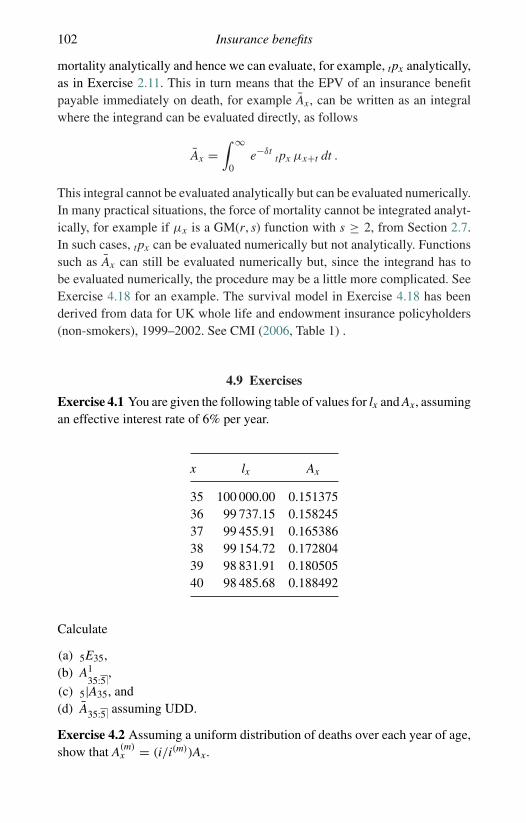
102 Insurance benefits
mortality analytically and hence we can evaluate, for example, tpx analytically,as in Exercise 2.11. This in turn means that the EPV of an insurance benefitpayable immediately on death, for example Ax, can be written as an integralwhere the integrand can be evaluated directly, as follows
Ax =∫ ∞
0e−δt
tpx µx+t dt .
This integral cannot be evaluated analytically but can be evaluated numerically.In many practical situations, the force of mortality cannot be integrated analyt-ically, for example if µx is a GM(r, s) function with s ≥ 2, from Section 2.7.In such cases, tpx can be evaluated numerically but not analytically. Functionssuch as Ax can still be evaluated numerically but, since the integrand has tobe evaluated numerically, the procedure may be a little more complicated. SeeExercise 4.18 for an example. The survival model in Exercise 4.18 has beenderived from data for UK whole life and endowment insurance policyholders(non-smokers), 1999–2002. See CMI (2006, Table 1) .
4.9 Exercises
Exercise 4.1 You are given the following table of values for lx and Ax, assumingan effective interest rate of 6% per year.
x lx Ax
35 100 000.00 0.15137536 99 737.15 0.15824537 99 455.91 0.16538638 99 154.72 0.17280439 98 831.91 0.18050540 98 485.68 0.188492
Calculate
(a) 5E35,(b) A1
35:5,
(c) 5|A35, and(d) A35:5 assuming UDD.
Exercise 4.2 Assuming a uniform distribution of deaths over each year of age,show that A(m)
x = (i/i(m))Ax.

4.9 Exercises 103
Exercise 4.3 A with-profit whole life insurance policy issued to a life agedexactly 30 has a basic sum insured of $100 000. The insurer assumes compoundreversionary bonuses at the rate of 3% will vest at the end of each policy year.Using the Standard Ultimate Survival Model, with interest at 5% per year,calculate the EPV of this benefit.
Exercise 4.4 (a) Show that
Ax:n =n−2∑k=0
vk+1k |qx + vn
n−1px .
(b) Compare this formula with formula (4.17) and comment on the differences.
Exercise 4.5 Show that
(IA(m))x = A(m)x + vpxA(m)
x+1 + 2pxv2A(m)
x+2 + · · ·
and explain this result intuitively.
Exercise 4.6 (a) Derive the following recursion formula for an n-year increas-ing term insurance:
(IA)1x:n = vqx + vpx
((IA) 1
x+1:n−1+ A 1
x+1:n−1
).
(b) Give an intuitive explanation of the formula in part (a).(c) You are given that (IA)50 = 4.99675, A 1
50:1= 0.00558, A51 = 0.24905
and i = 0.06. Calculate (IA)51 .
Exercise 4.7 You are given that Ax = 0.25, Ax+20 = 0.40, Ax:20 = 0.55 and
i = 0.03. Calculate 10 000Ax:20 using
(a) claims acceleration, and(b) UDD.
Exercise 4.8 Show that
(IA) 1x:n = (n + 1)A 1
x:n −n∑
k=1
A 1x:k
and explain this result intuitively.
Exercise 4.9 Show that Ax is a decreasing function of i, and explain this resultby general reasoning.

104 Insurance benefits
Exercise 4.10 Calculate A70 given that
A50:20 = 0.42247, A 150:20
= 0.14996, A50 = 0.31266.
Exercise 4.11 Under an endowment insurance issued to a life aged x, let Xdenote the present value of a unit sum insured, payable at the moment of deathor at the end of the n-year term.
Under a term insurance issued to a life aged x, let Y denote the present valueof a unit sum insured, payable at the moment of death within the n-year term.
Given that
V[X ] = 0.0052, vn = 0.3, npx = 0.8, E[Y ] = 0.04,
calculate V[Y ].Exercise 4.12 Show that if νy = − log py for y = x, x + 1, x + 2, . . ., thenunder the assumption of a constant force of mortality between integer ages,
Ax =∞∑
t=0
vttpx
νx+t(1 − vpx+t)
δ + νx+t.
Exercise 4.13 Let Z1 denote the present value of an n-year term insurancebenefit, issued to (x). Let Z2 denote the present value of a whole of life insurancebenefit, issued to the same life.
Express the covariance of Z1 and Z2 in actuarial functions, simplified as faras possible.
Exercise 4.14 You are given the following excerpt from a select life table.
[x] l[x] l[x]+1 l[x]+2 l[x]+3 lx+4 x + 4
[40] 100 000 99 899 99 724 99 520 99 288 44[41] 99 802 99 689 99 502 99 283 99 033 45[42] 99 597 99 471 99 268 99 030 98 752 46[43] 99 365 99 225 99 007 98 747 98 435 47[44] 99 120 98 964 98 726 98 429 98 067 48
Assuming an interest rate of 6% per year, calculate
(a) A[40]+1:4 ,(b) the standard deviation of the present value of a four-year term insurance,
deferred one year, issued to a newly selected life aged 40, with sum insured$100 000, payable at the end of the year of death, and
4.9 Exercises 105
(c) the probability that the present value of the benefit described in (b) is lessthan or equal to $85 000.
Exercise 4.15 (a) Describe in words the insurance benefits with the presentvalues given below.
(i) Z1 ={
20 vTx if Tx ≤ 15,10 vTx if Tx > 15.
(ii) Z2 =⎧⎨⎩
0 if Tx ≤ 5,10 vTx if 5 < Tx ≤ 15,10 v15 if Tx > 15.
(b) Write down in integral form the formula for the expected value for (i) Z1
and (ii) Z2.(c) Derive expressions in terms of standard actuarial functions for the expected
values of Z1 and Z2.(d) Derive an expression in terms of standard actuarial functions for the
covariance of Z1 and Z2.
Exercise 4.16 Suppose that Makeham’s law applies with A = 0.0001, B =0.00035 and c = 1.075. Assume also that the effective rate of interest is 6%per year.
(a) Use Excel and backward recursion in parts (i) and (ii).(i) Construct a table of values of Ax for integer ages, starting at x = 50.
(ii) Construct a table of values of A(4)x for x = 50, 50.25, 50.5, . . . . (Do
not use UDD for this.)(iii) Hence, write down the values of A50, A100, A(4)
50 and A(4)100.
(b) Use your values for A50 and A100 to estimate A(4)50 and A(4)
100 using the UDDassumption.
(c) Compare your estimated values for the A(4) functions (from (b)) with youraccurate values (from (a)). Comment on the differences.
Exercise 4.17 A life insurance policy issued to a life aged 50 pays $2000 atthe end of the quarter year of death before age 65 and $1000 at the end of thequarter year of death after age 65. Use the Standard Ultimate Survival Model,with interest at 5% per year, in the following.
(a) Calculate the EPV of the benefit.(b) Calculate the standard deviation of the present value of the benefit.(c) The insurer charges a single premium of $500. Assuming that the insurer
invests all funds at exactly 5% per year effective, what is the probability

106 Insurance benefits
that the policy benefit has greater value than the accumulation of the singlepremium?
Exercise 4.18 The force of mortality for a survival model is given by
µx = A + BCxDx2,
where
A = 3.5 × 10⁻⁴, B = 5.5 × 10⁻⁴, C = 1.00085, D = 1.0005.
(a) Calculate tp60 for t = 0, 1/40, 2/40, . . . , 2.Hint: Use the repeated Simpson’s rule.
(b) Calculate A160:2
using an effective rate of interest of 5% per year.
Hint: Use the repeated Simpson’s rule.
Answers to selected exercises
4.1 (a) 0.073594(b) 0.137503(c) 0.013872(d) 0.215182
4.3 $33 569.474.6 (c) 5.073074.7 (a) 5 507.44
(b) 5 507.464.10 0.597044.11 0.014.14 (a) 0.79267
(b) $7 519.71(c) 0.99825
4.16 (a) (iii) 0.33587, 0.87508, 0.34330, 0.89647(b) 0.34333, 0.89453
4.17 (a) $218.83(b) $239.73(c) 0.04054
4.18 (a) Selected values are 1/4p60 = 0.999031, p60 = 0.996049 and
2p60 = 0.991903(b) 0.007725
5
Annuities
5.1 Summary
In this chapter we derive expressions for the valuation and analysis of lifecontingent annuities. We consider benefit valuation for different payment fre-quencies, and we relate the valuation of annuity benefits to the valuation of therelated insurance benefits.
We consider how to calculate annuity valuation functions. If full survivalmodel information is available, then the calculation can be exact for benefitspayable at discrete time points, and as exact as required, using numerical inte-gration, for benefits payable continuously. Where we are calculating benefitspayable more frequently than annual (monthly or weekly, say) using only aninteger age life table, a very common situation in practice, then some approx-imation is required. We derive several commonly used approximations, usingthe UDD assumption and Woolhouse’s formula, and explore their accuracynumerically.
5.2 Introduction
We use the term life annuity to refer to a series of payments to (or from) anindividual as long as the individual is alive on the payment date. The paymentsare normally made at regular intervals and the most common situation is thatthe payments are of the same amount. The valuation of annuities is importantas annuities appear in the calculation of premiums (see Chapter 6), policyvalues (see Chapter 7) and pension benefits (see Chapter 9). The present valueof a life annuity is a random variable, as it depends on the future lifetime;however, we will use some results and notation from the valuation of annuities-certain, where there is no uncertainty in the term, so we start with a review ofthese.
107

108 Annuities
5.3 Review of annuities-certain
Recall that, for integer n,
an = 1 + v + v2 + · · · + vn−1 = 1 − vn
d(5.1)
denotes the present value of an annuity-certain of 1 payable annually in advancefor n years. Also
an = v + v2 + v3 + · · · + vn = an − 1 + vn
denotes the present value of an annuity-certain of 1 payable annually in arrearfor n years. Thirdly, for any n > 0,
an =∫ n
0vtdt = 1 − vn
δ(5.2)
denotes the present value of an annuity-certain payable continuously at rate 1per year for n years.
When payments of 1 per year are made every 1/m years in advance for nyears, in instalments of 1/m, the present value is
a(m)
n = 1m
(1 + v
1m + v
2m + · · · + vn− 1
m
)= 1 − vn
d (m)
and for payments made in arrears
a(m)
n = 1m
(v
1m + v
2m + · · · + vn
)= 1 − vn
i(m)= a(m)
n − 1m
(1 − vn) . (5.3)
In these equations for mthly annuities, we assume that n is an integer multipleof 1/m.
5.4 Annual life annuities
The annual life annuity is paid once each year, conditional on the survival of alife (the annuitant) to the payment date. If the annuity is to be paid throughoutthe annuitant’s life, it is called a whole life annuity. If there is to be a specifiedmaximum term, it is called a term or temporary annuity.
Annual annuities are quite rare. We would more commonly see annuitiespayable monthly or even weekly. However, the annual annuity is still importantin the situation where we do not have full information about mortality betweeninteger ages, for example because we are working with an integer age life table.Also, the development of the valuation functions for the annual annuity is agood starting point before considering more complex payment patterns.

5.4 Annual life annuities 109
As with the insurance functions, we are primarily interested in the EPV of acash flow, and we also identify the present value random variables in terms ofthe future lifetime random variables from Chapters 2 and 4, specifically, Tx, Kx
and K (m)x .
5.4.1 Whole life annuity-due
Consider first an annuity of 1 per year payable annually in advance through-out the lifetime of an individual now aged x. The life annuity with paymentsin advance is known as a whole life annuity-due. The first payment occursimmediately, the second in one year from now, provided that (x) is alive then,and payments follow at annual intervals with each payment conditional on thesurvival of (x) to the payment date. In Figure 5.1 we show the payments andassociated probabilities and discount functions in a time-line diagram.
We note that if (x) were to die between ages x + k and x + k + 1, for somepositive integer k, then annuity payments would be made at times 0, 1, 2, . . . , k,for a total of k + 1 payments. We defined Kx such that the death of (x) occursbetween x+Kx and x+Kx +1, so, the number of payments is Kx +1, includingthe initial payment. This means that, for k = 0, 1, 2, . . ., the present value ofthe annuity is ak+1 if Kx = k. Thus, using equation (5.1), the present valuerandom variable for the annuity payment series, Y , say, can be written as
Y = aKx+1 = 1 − vKx+1
d.
There are three useful ways to derive formulae for calculating the expectedvalue of this present value random variable.
First, the mean and variance can be found from the mean and variance ofvKx+1, which were derived in Section 4.4.2. For the expected value of Y , which
Time 0 1 2 3
. . .
Amount 1 1 1 1
Discount 1 v v2 v3
Probability 1 px 2px 3px
Figure 5.1 Time-line diagram for whole life annuity-due.

110 Annuities
is denoted ax , we have
ax = E
[1 − vKx+1
d
]= 1 − E[vKx+1]
d.
That is,
ax = 1 − Ax
d. (5.4)
This is a useful approach, as it also immediately gives us the variance of Y as
V[Y ] = V
[1 − vKx+1
d
]
= 1
d2V[vKx+1]
=2Ax − A2
x
d2. (5.5)
Secondly, we may use the indicator random variable approach from Section4.6. The condition for the payment at k, say, is that (x) is alive at age x + k, thatis, that Tx > k. The present value random variable can be expressed as
Y = I(Tx > 0) + v I(Tx > 1) + v2 I(Tx > 2) + v3 I(Tx > 3) + · · · (5.6)
and the EPV of the annuity is the sum of the expected values of the individualterms. Recall that E[I(Tx > t)] = Pr[Tx > t] = tpx, so that
ax = 1 + v px + v22px + v3
3px + · · · ,
that is
ax =∞∑
k=0
vkkpx . (5.7)
This is a very useful equation for ax. However, this approach does not lead touseful expressions for the variance and higher moments of Y . This is becausethe individual terms in expression (5.6) are dependent random variables.
Finally, we can work from the probability function for Kx, that is usingPr[Kx = k] = k |qx, so that
ax =∞∑
k=0
ak+1 k |qx . (5.8)

5.4 Annual life annuities 111
This is less used in practice than equations (5.4) and (5.7). The differencebetween the formulations for ax in equations (5.7) and (5.8) is that in equation(5.7) the summation is taken over the possible payment dates, and in equation(5.8) the summation is taken over the possible years of death.
Example 5.1 Show that equations (5.7) and (5.8) are equivalent – that is,show that
∞∑k=0
ak+1 k |qx =∞∑
k=0
vkkpx .
Solution 5.1 We can show this by using
ak+1 =k∑
t=0
vt
and
∞∑k=t
k |qx =∞∑
k=t
(kpx − k+1px) = tpx .
Then
∞∑k=0
ak+1 k |qx =∞∑
k=0
k∑t=0
vtk |qx
= qx + (1 + v) 1|1qx + (1 + v + v2) 2|1qx
+ (1 + v + v2 + v3) 3|1qx + · · · .
Changing the order of summation on the right-hand side (that is, collectingtogether terms in powers of v) gives
∞∑k=0
k∑t=0
vtk |qx =
∞∑t=0
∞∑k=t
vtk |qx
=∞∑
t=0
vt∞∑
k=t
k |qx
=∞∑
t=0
vttpx
as required. �

112 Annuities
5.4.2 Term annuity-due
Now suppose we wish to value a term annuity-due of 1 per year. We assumethe annuity is payable annually to a life now aged x for a maximum of n years.Thus, payments are made at times k = 0, 1, 2, . . . , n − 1, provided that (x) hassurvived to age x + k. The present value of this annuity is Y , say, where
Y ={
aKx+1 if Kx = 0, 1, . . . , n − 1,
an if Kx ≥ n.
that is
Y = amin(Kx+1, n)= 1 − vmin(Kx+1, n)
d.
The EPV of this annuity is denoted ax:n .We have seen the random variable vmin(Kx+1, n) before, in Section 4.4.7, where
the EPV Ax:n is derived. Thus, the EPV of the annuity can be determined as
ax:n = E[Y ] = 1 − E[vmin(Kx+1, n)]d
that is,
ax:n = 1 − Ax:n
d. (5.9)
The time-line for the term annuity-due cash flow is shown in Figure 5.2. Noticethat, because the payments are made in advance, there is no payment due attime n, the end of the annuity term.
Using Figure 5.2, and summing the EPVs of the individual payments, wehave
ax:n = 1 + v px + v22px + v3
3px + · · · + vn−1n−1px
Time 0 1 2 3
. . . . . .
n-1 n
Amount 1 1 1 1 1
Discount 1 v v2 v3 vn−1
Probability 1 px 2px 3px n−1px
Figure 5.2 Time-line diagram for term life annuity-due.

5.4 Annual life annuities 113
that is
ax:n =n−1∑t=0
vttpx . (5.10)
Also, we can write the EPV as
ax:n =n−1∑k=0
ak+1 k |qx + npx an
adapting equation (5.8) above. The second term here arises from the secondterm in the definition of Y – that is, if the annuitant survives for the full term,then the payments constitute an n-year annuity.
5.4.3 Whole life immediate annuity
Now consider a whole life annuity of 1 per year payable in arrear, conditionalon the survival of (x) to the payment dates. We use the term immediate annuityto refer to an annuity under which payments are made at the end of the timeperiods, rather than at the beginning. The actuarial notation for the EPV of thisannuity is ax, and the time-line for the annuity cash flow is shown in Figure 5.3.
Let Y ∗ denote the present value random variable for the whole life immediateannuity. Using the indicator random variable approach we have
Y ∗ = v I(Tx > 1) + v2 I(Tx > 2) + v3 I(Tx > 3) + v4 I(Tx > 4) + · · · .
We can see from this expression and from the time-line, that the differencein present value between the annuity-due and the immediate annuity payablein arrear is simply the first payment under the annuity-due, which, under theannuity-due, is assumed to be paid at time t = 0 with certainty.
Time 0 1 2 3
. . .
Amount 1 1 1
Discount v v2 v3
Probability px 2px 3px
Figure 5.3 Time-line diagram for whole life immediate annuity.
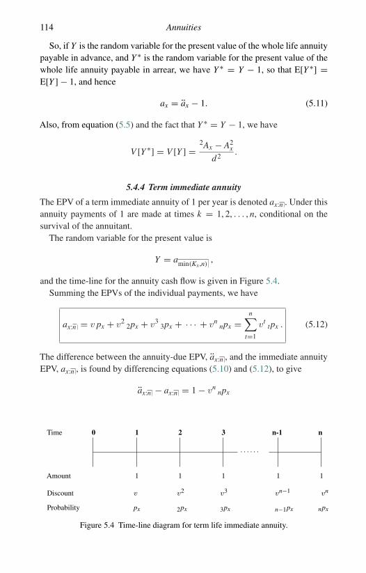
114 Annuities
So, if Y is the random variable for the present value of the whole life annuitypayable in advance, and Y ∗ is the random variable for the present value of thewhole life annuity payable in arrear, we have Y ∗ = Y − 1, so that E[Y ∗] =E[Y ] − 1, and hence
ax = ax − 1. (5.11)
Also, from equation (5.5) and the fact that Y ∗ = Y − 1, we have
V [Y ∗] = V [Y ] =2Ax − A2
x
d2.
5.4.4 Term immediate annuity
The EPV of a term immediate annuity of 1 per year is denoted ax:n . Under thisannuity payments of 1 are made at times k = 1, 2, . . . , n, conditional on thesurvival of the annuitant.
The random variable for the present value is
Y = amin(Kx ,n),
and the time-line for the annuity cash flow is given in Figure 5.4.Summing the EPVs of the individual payments, we have
ax:n = v px + v22px + v3
3px + · · · + vnnpx =
n∑t=1
vttpx . (5.12)
The difference between the annuity-due EPV, ax:n , and the immediate annuityEPV, ax:n , is found by differencing equations (5.10) and (5.12), to give
ax:n − ax:n = 1 − vnnpx
Time 0 1 2 3
. . . . . .
n-1 n
Amount 1 1 1 1 1
Discount v v2 v3 vn−1 vn
Probability px 2px 3px n−1px npx
Figure 5.4 Time-line diagram for term life immediate annuity.
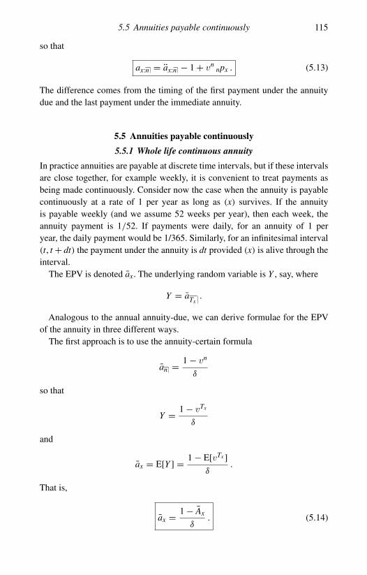
5.5 Annuities payable continuously 115
so that
ax:n = ax:n − 1 + vnnpx . (5.13)
The difference comes from the timing of the first payment under the annuitydue and the last payment under the immediate annuity.
5.5 Annuities payable continuously
5.5.1 Whole life continuous annuity
In practice annuities are payable at discrete time intervals, but if these intervalsare close together, for example weekly, it is convenient to treat payments asbeing made continuously. Consider now the case when the annuity is payablecontinuously at a rate of 1 per year as long as (x) survives. If the annuityis payable weekly (and we assume 52 weeks per year), then each week, theannuity payment is 1/52. If payments were daily, for an annuity of 1 peryear, the daily payment would be 1/365. Similarly, for an infinitesimal interval(t, t + dt) the payment under the annuity is dt provided (x) is alive through theinterval.
The EPV is denoted ax. The underlying random variable is Y , say, where
Y = aTx.
Analogous to the annual annuity-due, we can derive formulae for the EPVof the annuity in three different ways.
The first approach is to use the annuity-certain formula
an = 1 − vn
δ
so that
Y = 1 − vTx
δ
and
ax = E[Y ] = 1 − E[vTx ]δ
.
That is,
ax = 1 − Ax
δ. (5.14)

116 Annuities
Using this formulation for the random variable Y , we can also directly derivethe variance for the continuous annuity present value from the variance for thecontinuous insurance benefit
V[Y ] = V
[1 − vTx
δ
]=
2Ax − A2x
δ2.
The second approach is to use the sum (here an integral) of the product of theamount paid in each infinitesimal interval (t, t + dt), the discount factor for theinterval and the probability that the payment is made. For each such interval,the amount is dt, the discount factor is e−δt and the probability of payment is
tpx, giving
ax =∫ ∞
0e−δt
tpx dt . (5.15)
We remark that this EPV can also be derived using indicator random variablesby expressing the present value as
Y =∫ ∞
0e−δt I(Tx > t) dt .
The development of formula (5.15) is illustrated in Figure 5.5; we show thecontribution to the integral from the contingent annuity payment made in aninfinitesimal interval of time (t, t + dt). The interval is so small that paymentscan be treated as being made exactly at t.
Finally, we can directly write down the EPV from the distribution of Tx as
ax =∫ ∞
0at tpx µx+t dt.
Time 0
. . .
t
� �
t+dt
Amount dt
Discount e−δt
Probability tpx
Figure 5.5 Time-line diagram for continuous whole life annuity.

5.5 Annuities payable continuously 117
We can evaluate this using integration by parts, noting that if we differentiateequation (5.2) we get
d
dtat = vt = e−δt .
Then
ax =∫ ∞
0at
d
dt(−tpx)dt
= −(
at tpx|∞0 −∫ ∞
0tpx e−δtdt
)
=∫ ∞
0e−δt
tpx dt .
When δ = 0, we see that ax is equal to◦ex, the complete expectation of life.
5.5.2 Term continuous annuity
The term continuous life annuity present value random variable
amin(Tx ,n)= 1 − vmin(Tx ,n)
δ
has EPV denoted by ax:n . Analogous to the term annuity-due, we have threeexpressions for this EPV.
Using results for endowment insurance functions from Section 4.4.7, we have
ax:n = 1 − Ax:n
δ. (5.16)
Using the indicator random variable approach we have
ax:n =∫ n
0e−δt
tpx dt , (5.17)
and taking the expected value of the present value random variable we obtain
ax:n =∫ n
0at tpx µx+t dt + an npx.
One way to understand the difference between the second and third approachesis to see that in the second approach we integrate over the possible paymentdates, and in the third approach we integrate over the possible dates of death.The third approach is generally the least useful in practice.
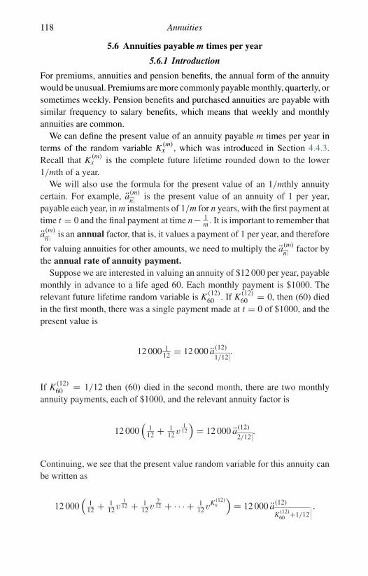
118 Annuities
5.6 Annuities payable m times per year
5.6.1 Introduction
For premiums, annuities and pension benefits, the annual form of the annuitywould be unusual. Premiums are more commonly payable monthly, quarterly, orsometimes weekly. Pension benefits and purchased annuities are payable withsimilar frequency to salary benefits, which means that weekly and monthlyannuities are common.
We can define the present value of an annuity payable m times per year interms of the random variable K (m)
x , which was introduced in Section 4.4.3.Recall that K (m)
x is the complete future lifetime rounded down to the lower1/mth of a year.
We will also use the formula for the present value of an 1/mthly annuitycertain. For example, a(m)
n is the present value of an annuity of 1 per year,payable each year, in m instalments of 1/m for n years, with the first payment attime t = 0 and the final payment at time n− 1
m . It is important to remember that
a(m)
n is an annual factor, that is, it values a payment of 1 per year, and therefore
for valuing annuities for other amounts, we need to multiply the a(m)
n factor bythe annual rate of annuity payment.
Suppose we are interested in valuing an annuity of $12 000 per year, payablemonthly in advance to a life aged 60. Each monthly payment is $1000. Therelevant future lifetime random variable is K (12)
60 . If K (12)60 = 0, then (60) died
in the first month, there was a single payment made at t = 0 of $1000, and thepresent value is
12 000 112 = 12 000 a(12)
1/12.
If K (12)60 = 1/12 then (60) died in the second month, there are two monthly
annuity payments, each of $1000, and the relevant annuity factor is
12 000(
112 + 1
12v112
)= 12 000 a(12)
2/12.
Continuing, we see that the present value random variable for this annuity canbe written as
12 000(
112 + 1
12v112 + 1
12v212 + · · · + 1
12vK (12)x)
= 12 000 a(12)
K (12)60 +1/12
.
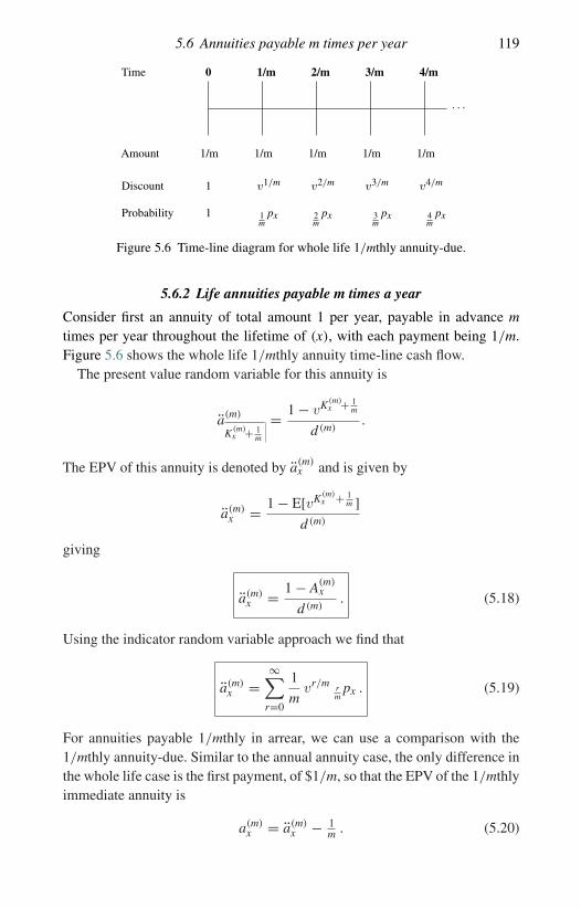
5.6 Annuities payable m times per year 119
Time 0 1/m 2/m 3/m 4/m
. . .
Amount 1/m 1/m 1/m 1/m 1/m
Discount 1 v1/m v2/m v3/m v4/m
Probability 1 1m
px 2m
px 3m
px 4m
px
Figure 5.6 Time-line diagram for whole life 1/mthly annuity-due.
5.6.2 Life annuities payable m times a year
Consider first an annuity of total amount 1 per year, payable in advance mtimes per year throughout the lifetime of (x), with each payment being 1/m.Figure 5.6 shows the whole life 1/mthly annuity time-line cash flow.
The present value random variable for this annuity is
a(m)
K (m)x + 1
m
= 1 − vK (m)x + 1
m
d (m).
The EPV of this annuity is denoted by a(m)x and is given by
a(m)x = 1 − E[vK (m)
x + 1m ]
d (m)
giving
a(m)x = 1 − A(m)
x
d (m). (5.18)
Using the indicator random variable approach we find that
a(m)x =
∞∑r=0
1
mvr/m r
mpx . (5.19)
For annuities payable 1/mthly in arrear, we can use a comparison with the1/mthly annuity-due. Similar to the annual annuity case, the only difference inthe whole life case is the first payment, of $1/m, so that the EPV of the 1/mthlyimmediate annuity is
a(m)x = a(m)
x − 1m . (5.20)
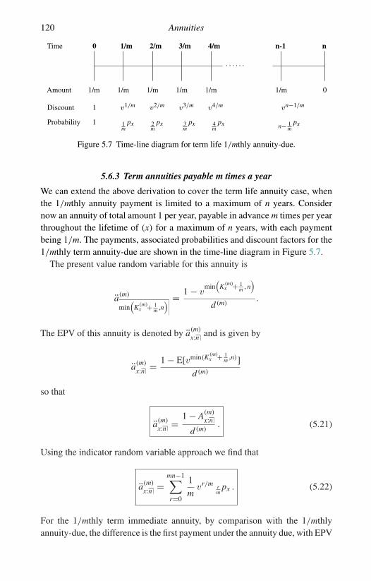
120 Annuities
Time 0 1/m 2/m 3/m 4/m
. . . . . .
n-1 n
Amount 1/m 1/m 1/m 1/m 1/m 1/m 0
Discount 1 v1/m v2/m v3/m v4/m vn−1/m
Probability 1 1m
px 2m
px 3m
px 4m
px n− 1m
px
Figure 5.7 Time-line diagram for term life 1/mthly annuity-due.
5.6.3 Term annuities payable m times a year
We can extend the above derivation to cover the term life annuity case, whenthe 1/mthly annuity payment is limited to a maximum of n years. Considernow an annuity of total amount 1 per year, payable in advance m times per yearthroughout the lifetime of (x) for a maximum of n years, with each paymentbeing 1/m. The payments, associated probabilities and discount factors for the1/mthly term annuity-due are shown in the time-line diagram in Figure 5.7.
The present value random variable for this annuity is
a(m)
min(
K (m)x + 1
m ,n) = 1 − v
min(
K (m)x + 1
m , n)
d (m).
The EPV of this annuity is denoted by a(m)
x:n and is given by
a(m)
x:n = 1 − E[vmin(K (m)x + 1
m ,n)]d (m)
so that
a(m)
x:n = 1 − A(m)
x:n
d (m). (5.21)
Using the indicator random variable approach we find that
a(m)
x:n =mn−1∑r=0
1
mvr/m r
mpx . (5.22)
For the 1/mthly term immediate annuity, by comparison with the 1/mthlyannuity-due, the difference is the first payment under the annuity due, with EPV
5.7 Comparison of annuities by payment frequency 121
1/m, and the final payment under the immediate annuity, with EPV 1mvn
npx,so that
a(m)
x:n = a(m)
x:n − 1
m
(1 − vn
npx)
. (5.23)
This is analogous to the result in equation (5.3) for the annuity-certain. Fur-ther, by setting m = 1 in equations (5.19) and (5.22) we obtain equations(5.7) and (5.10) for ax and ax:n . Also, by letting m → ∞ in equations (5.19)and (5.22) we obtain equations (5.15) and (5.17) for continuous annuities, ax
and ax:n .We can derive expressions for the EPV of other types of annuity payable m
times per year, and indeed we can also find higher moments of present valuesas we did for annuities payable annually.
5.7 Comparison of annuities by payment frequency
In Table 5.1 we show values for ax, a(4)x , ax, a(4)
x and ax for x = 20, 40, 60and 80, using the Standard Ultimate Survival Model from Section 4.3, withinterest of 5% per year. Using equations (5.11), (5.20), (5.15), (5.19) and (5.7),we obtain the values shown in Table 5.1. We observe that each set of valuesdecreases with age, reflecting the shorter expected life span as age increases.We also have, for each age, the ordering
ax < a(4)x < ax < a(4)
x < ax .
There are two reasons for this ordering.
• While the life is alive, the payments in each year sum to 1 under each annuity,but on average, the payments under the annuity-due are paid earlier. The timevalue of money means that the value of an annuity with earlier payments willbe higher than an annuity with later payments, for interest rates greater thanzero, so the annuity values are in increasing order from the latest averagepayment date (ax payments are at each year end) to the earliest (ax paymentsare at the start of each year).
• In the year that (x) dies, the different annuities pay different amounts. Underthe annual annuity-due the full year’s payment of $1 is paid, as the life isalive at the payment date at the start of the year. Under the annual immediateannuity, in the year of death no payment is made as the life does not surviveto the payment date at the year end. For the mthly and continuous annuities,less than the full year’s annuity may be paid in the year of death.
For example, suppose the life dies after seven months. Under the annualannuity due, the full annuity payment is made for that year, at the start of

122 Annuities
Table 5.1. Values of ax , a(4)x , ax , a(4)
x and ax.
x ax a(4)x ax a(4)
x ax
20 18.966 19.338 19.462 19.588 19.96640 17.458 17.829 17.954 18.079 18.45860 13.904 14.275 14.400 14.525 14.90480 7.548 7.917 8.042 8.167 8.548
the year. Under the quarterly annuity due, three payments are made, each of1/4 of the total annual amount, at times 0, 1/4 and 1/2. The first year’s finalpayment, due at time 3/4, is not made, as the life does not survive to thatdate. Under the continuous annuity, the life collects 7/12ths of the annualamount. Under the quarterly immediate annuity, the life collects payments attimes 1/4, 1/2, and misses the two payments due at times 3/4 and 1. Underthe annual immediate annuity, the life collects no annuity payments at all, asthe due date is the year end.
This second point explains why we cannot make a simple interest adjustment torelate the annuity-due and the continuous annuity. The situation here is differentfrom the insurance benefits; Ax and A(4)
x , for example, both value a paymentof $1 in the year of death, Ax at the end of the year, and A(4)
x at the end of thequarter year of death. There is no difference in the amount of the payment, onlyin the timing. For the annuities, the difference between ax and a(4)
x arises fromdifferences in both cashflow timing and benefit amount in the year of death.
We also note from Table 5.1 that the ax values are close to being half-waybetween ax and ax, suggesting the approximation ax ≈ ax + 1
2 . We will see inSection 5.11.3 that there is indeed a way of calculating an approximation to ax
from ax, but it involves an extra adjustment term to ax.
Example 5.2 Using the Standard Ultimate Survival Model, with 5% per yearinterest, calculate values of ax:10 , a(4)
x:10, ax:10 , a(4)
x:10and ax:10 for x = 20, 40,
60 and 80, and comment.
Solution 5.2 Using equations (5.10), (5.12), (5.17), (5.23) and (5.22) withn = 10 we obtain the values shown in Table 5.2.
We note that for a given annuity function, the values do not vary greatly withage, since the probability of death in a 10-year period is small. That means,for example, that the second term in equation (5.10) is much greater than the
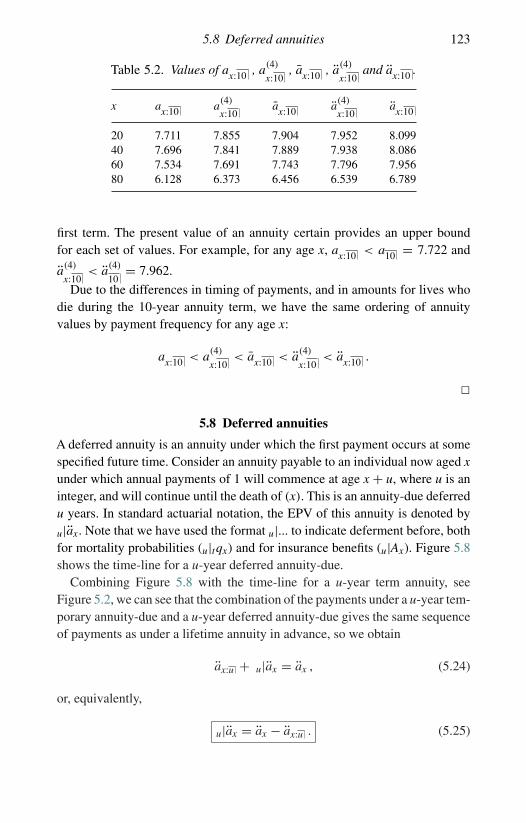
5.8 Deferred annuities 123
Table 5.2. Values of ax:10 , a(4)
x:10, ax:10 , a(4)
x:10and ax:10 .
x ax:10 a(4)
x:10ax:10 a(4)
x:10ax:10
20 7.711 7.855 7.904 7.952 8.09940 7.696 7.841 7.889 7.938 8.08660 7.534 7.691 7.743 7.796 7.95680 6.128 6.373 6.456 6.539 6.789
first term. The present value of an annuity certain provides an upper boundfor each set of values. For example, for any age x, ax:10 < a10 = 7.722 and
a(4)
x:10< a(4)
10= 7.962.
Due to the differences in timing of payments, and in amounts for lives whodie during the 10-year annuity term, we have the same ordering of annuityvalues by payment frequency for any age x:
ax:10 < a(4)
x:10< ax:10 < a(4)
x:10< ax:10 .
�
5.8 Deferred annuities
A deferred annuity is an annuity under which the first payment occurs at somespecified future time. Consider an annuity payable to an individual now aged xunder which annual payments of 1 will commence at age x + u, where u is aninteger, and will continue until the death of (x). This is an annuity-due deferredu years. In standard actuarial notation, the EPV of this annuity is denoted by
u|ax. Note that we have used the format u|... to indicate deferment before, bothfor mortality probabilities (u|tqx) and for insurance benefits (u|Ax). Figure 5.8shows the time-line for a u-year deferred annuity-due.
Combining Figure 5.8 with the time-line for a u-year term annuity, seeFigure 5.2, we can see that the combination of the payments under a u-year tem-porary annuity-due and a u-year deferred annuity-due gives the same sequenceof payments as under a lifetime annuity in advance, so we obtain
ax:u + u|ax = ax , (5.24)
or, equivalently,
u|ax = ax − ax:u . (5.25)

124 Annuities
Time 0 1 2
. . . . . . . . .
u-1 u u+1
Amount 0 0 0 0 1 1
Discount 1 v1 v2 vu−1 vu vu+1
Probability 1 1px 2px u−1px upx u+1px
Figure 5.8 Time-line diagram for deferred annual annuity-due.
Similarly, the EPV of an annuity payable continuously at rate 1 per year to alife now aged x, commencing at age x + u, is denoted by u|ax and given by
u|ax = ax − ax:u .
Summing the EPVs of the individual payments for the deferred whole lifeannuity-due gives
u|ax = vuupx + vu+1
u+1px + vu+2u+2px + · · ·
= vuupx
(1 + v px+u + v2
2px+u + · · ·)
so that
u|ax = vuupx ax+u = uEx ax+u . (5.26)
We see again that the pure endowment function acts like a discount function. Infact, we can use the uEx function to find the EPV of any deferred benefit. Forexample, for a deferred term immediate annuity,
u|ax:n = uEx ax+u:n ,
and for an annuity-due payable 1/mthly,
u|a(m)x = uEx a(m)
x+u . (5.27)
This result can be helpful when working with tables. Suppose we have availablea table of whole life annuity-due values, say ax, along with the life table functionlx, and we need the term annuity value ax:n . Then, using equations (5.24) and(5.26), we have
ax:n = ax − vnnpx ax+n . (5.28)

5.9 Guaranteed annuities 125
For 1/mthly payments, the corresponding formula is
a(m)
x:n = a(m)x − vn
npx a(m)x+n . (5.29)
Example 5.3 Let Y1, Y2 and Y3 denote present value random variables for au-year deferred whole life annuity-due, a u-year term annuity-due and a wholelife annuity-due, respectively. Show that Y3 = Y1 + Y2. Assume annualpayments.
Solution 5.3 The present value random variable for a u-year deferred wholelife annuity-due, with annual payments is
Y1 ={
0 if Kx ≤ u − 1,vuaKx+1−u if Kx ≥ u,
={
0 if Kx ≤ u − 1,aKx+1 − au if Kx ≥ u.
(5.30)
From Section 5.4.2 we have
Y2 ={
aKx+1 if Kx ≤ u − 1,
au if Kx ≥ u.
Hence
Y1 + Y2 ={
aKx+1 if Kx ≤ u − 1,
aKx+1 if Kx ≥ u,= aKx+1 = Y3 ,
as required. �
We use deferred annuities as building blocks in later sections, noting that ann-year term annuity, with any payment frequency, can be decomposed as thesum of n deferred annuities, each with term 1 year. So, for example,
ax:n =n−1∑u=0
u|ax:1 . (5.31)
5.9 Guaranteed annuities
A common feature of pension benefits is that the pension annuity is guaranteedto be paid for some period even if the life dies before the end of the period. Forexample, a pension benefit payable to a life aged 65, might be guaranteed for5, 10 or even 15 years.
Suppose an annuity-due of 1 per year is paid annually to (x), and is guaranteedfor a period of n years. Then the payment due at k years is paid whether or not
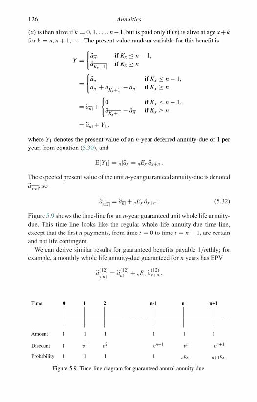
126 Annuities
(x) is then alive if k = 0, 1, . . . , n−1, but is paid only if (x) is alive at age x +kfor k = n, n + 1, . . . . The present value random variable for this benefit is
Y ={
an if Kx ≤ n − 1,aKx+1 if Kx ≥ n
={
an if Kx ≤ n − 1,an + aKx+1 − an if Kx ≥ n
= an +{
0 if Kx ≤ n − 1,aKx+1 − an if Kx ≥ n
= an + Y1 ,
where Y1 denotes the present value of an n-year deferred annuity-due of 1 peryear, from equation (5.30), and
E[Y1] = n|ax = nEx ax+n .
The expected present value of the unit n-year guaranteed annuity-due is denotedax:n , so
ax:n = an + nEx ax+n . (5.32)
Figure 5.9 shows the time-line for an n-year guaranteed unit whole life annuity-due. This time-line looks like the regular whole life annuity-due time-line,except that the first n payments, from time t = 0 to time t = n − 1, are certainand not life contingent.
We can derive similar results for guaranteed benefits payable 1/mthly; forexample, a monthly whole life annuity-due guaranteed for n years has EPV
a(12)
x:n= a(12)
n + nEx a(12)x+n .
Time 0 1 2
. . . . . . . . .
n-1 n n+1
Amount 1 1 1 1 1 1
Discount 1 v1 v2 vn−1 vn vn+1
Probability 1 1 1 1 npx n+1px
Figure 5.9 Time-line diagram for guaranteed annual annuity-due.

5.10 Increasing annuities 127
Example 5.4 Apension plan member is entitled to a benefit of $1000 per month,in advance, for life from age 65, with no guarantee. She can opt to take a lowerbenefit, with a 10-year guarantee. The revised benefit is calculated to have equalEPV at age 65 to the original benefit. Calculate the revised benefit using theStandard Ultimate Survival Model, with interest at 5% per year.
Solution 5.4 Let B denote the revised monthly benefit. To determine B wemust equate the EPV of the original benefit with that of the revised benefit.The resulting equation of EPVs is usually called an equation of value. Ourequation of value is
12 000a(12)65 = 12 B a(12)
65:10
where a(12)65 = 13.0870, and
a(12)
65:10= a(12)
10+ 10p65v
10a(12)75 = 13.3791.
Thus, the revised monthly benefit is B = $978.17. So the pension plan membercan gain the security of the 10-year guarantee at a cost of a reduction of $21.83per month in her pension. �
5.10 Increasing annuities
In the previous sections we have considered annuities with level payments.Some of the annuities which arise in actuarial work are not level. For example,annuity payments may increase over time. For these annuities, we are gener-ally interested in determining the EPV, and are rarely concerned with highermoments. To calculate higher moments it is generally necessary to use firstprinciples, and a computer.
The best approach for calculating the EPV of non-level annuities is to usethe indicator random variable, or time-line, approach – that is, sum over allthe payment dates the product of the amount of the payment, the probability ofpayment (that is, the probability that the life survives to the payment date) andthe appropriate discount factor.
5.10.1 Arithmetically increasing annuities
We first consider annuities under which the amount of the annuity paymentincreases arithmetically with time. Consider an increasing annuity-due wherethe amount of the annuity is t + 1 at times t = 0, 1, 2, . . . , n − 1 provided that(x) is alive at time t. The time-line is shown in Figure 5.10.

128 Annuities
Time 0 1 2 3 4
. . .
Amount 1 2 3 4 5
Discount 1 v1 v2 v3 v4
Probability 1 1px 2px 3px 4px
Figure 5.10 Time-line diagram for arithmetically increasing annual annuity-due.
The EPV of the annuity is denoted by (I a)x in standard actuarial notation.From the diagram we see that
(I a)x =∞∑
t=0
vt(t + 1) tpx . (5.33)
Similarly, if the annuity is payable for a maximum of n payments rather than forthe whole life of (x), the EPV, denoted by (I a)x:n in standard actuarial notation,is given by
(I a)x:n =n−1∑t=0
vt(t + 1) tpx . (5.34)
If the annuity is payable continuously, with the payments increasing by 1 ateach year end, so that the rate of payment in the tth year is constant and equalto t, for t = 1, 2, . . . , n, then we may consider the n-year temporary annuity asa sum of one-year deferred annuities. By analogy with formula (5.31), the EPVof this annuity, denoted in standard actuarial notation by (I a)x:n , is
(I a)x:n =n−1∑m=0
(m + 1) m|ax:1 .
We also have standard actuarial notation for the continuous annuity under whichthe rate of payment at time t > 0 is t; that is, the rate of payment is changingcontinuously. The notation for the EPV of this annuity is (I a)x if it is a wholelife annuity, and (I a)x:n if it is a term annuity. For every infinitesimal interval,(t, t + dt), the amount of annuity paid, if the life (x) is still alive, is t dt, theprobability of payment is tpx and the discount function is e−δ t = vt . Thetime-line is shown in Figure 5.11.

5.10 Increasing annuities 129
Time 0
. . .
t
� �
t+dt
Amount t dt
Discount e−δt
Probability tpx
Figure 5.11 Time-line diagram for increasing continuous whole life annuity.
To determine the EPV we integrate over all the possible intervals (t, t + dt),so that
(I a)x:n =∫ n
0t e−δt
tpx dt. (5.35)
5.10.2 Geometrically increasing annuities
An annuitant may be interested in purchasing an annuity that increases geomet-rically, to offset the effect of inflation on the purchasing power of the income.The approach is similar to the geometrically increasing insurance benefit whichwas considered in Examples 4.8 and 4.9.
Example 5.5 Consider an annuity-due with annual payments where the amountof the annuity is (1 + j)t at times t = 0, 1, 2, . . . , n − 1 provided that (x) is aliveat time t. Derive an expression for the EPV of this benefit, and simplify as faras possible.
Solution 5.5 First, consider the time-line diagram in Figure 5.12.By summing the product of
• the amount of the payment at time t,• the discount factor for time t, and• the probability that the payment is made at time t,
over all possible values of t, we obtain the EPV as
n−1∑t=0
(1 + j)t vttpx = ax:n i∗

130 Annuities
Time 0 1 2 3 4
……
Amount 1 (1 + j) (1 + j)2 (1 + j)3 (1 + j)4
Discount 1 v1 v2 v3 v4
Probability 1 1px 2px 3px 4px
Figure 5.12 Time-line diagram for geometrically increasing annual annuity-due.
where ax:n i∗ is the EPV of a term annuity-due evaluated at interest rate i∗ where
i∗ = 1 + i
1 + j− 1 = i − j
1 + j.
�
5.11 Evaluating annuity functions
If we have full information about the survival function for a life, then we can usesummation or numerical integration to compute the EPV of any annuity. Often,though, we have only integer age information, for example when the survivalfunction information is derived from a life table with integer age informationonly. In this section we consider how to evaluate the EPV of 1/mthly andcontinuous annuities given only the EPVs of annuities at integer ages. Forexample, we may have ax values for integer x. We present two methods thatare commonly used, and we explore the accuracy of these methods for a fairlytypical (Makeham) mortality model. First we consider recursive calculation ofEPVs of annuities.
5.11.1 Recursions
In a spreadsheet, with values for tpx available, we may calculate ax usinga backward recursion. We assume that there is an integer limiting age, ω,so that qω−1 = 1. First, we set aω−1 = 1. The backward recursion forx = ω−2, ω−3, ω−4, . . . is
ax = 1 + v px ax+1 (5.36)
since
ax = 1 + v px + v22px + v3
3px + · · ·= 1 + v px
(1 + v px+1 + v2
2px+1 + · · ·)
= 1 + v px ax+1.

5.11 Evaluating annuity functions 131
Similarly, for the 1/mthly annuity due,
a(m)ω−1/m = 1
m ,
and the backward recursion for x = ω− 2m , ω− 3
m , ω− 4m , . . . is
a(m)x = 1
m + v1m 1
mpx a(m)
x+ 1m
. (5.37)
We can calculate EPVs for term annuities and deferred annuities from the wholelife annuity EPVs, using, for example, equations (5.24) and (5.26).
To find the EPV of an annuity payable continuously we can use numericalintegration. Note, however, that Woolhouse’s formula, which is described inSection 5.11.3, gives an excellent approximation to 1/mthly and continuousannuity EPVs.
5.11.2 Applying the UDD assumption
We consider the evaluation of a(m)
x:n under the assumption of a uniform distribu-tion of deaths (UDD). The indication from Table 4.6 is that, in terms of EPVsfor insurance benefits, UDD offers a reasonable approximation at younger ages,but may not be sufficiently accurate at older ages.
From Section 4.5.1 recall the results from equations (4.27) and (4.26) that,under the UDD assumption,
A(m)x = i
i(m)Ax and Ax = i
δAx .
We also know, from equations (5.4), (5.18) and (5.14) in this chapter that forany survival model
ax = 1 − Ax
d, a(m)
x = 1 − A(m)x
d (m)and ax = 1 − Ax
δ.
Now, putting these equations together we have
a(m)x = 1 − A(m)
x
d (m)
= 1 − ii(m) Ax
d (m)using UDD
= i(m) − iAx
i(m) d (m)

132 Annuities
= i(m) − i(1 − dax)
i(m) d (m)using (5.4)
= id
i(m) d (m)ax − i − i(m)
i(m) d (m)
= α(m) ax − β(m)
where
α(m) = id
i(m) d (m)and β(m) = i − i(m)
i(m) d (m). (5.38)
For continuous annuities we can let m → ∞, so that
ax = id
δ2ax − i − δ
δ2.
For term annuities, starting from equation (5.29) we have,
a(m)
x:n = a(m)x − vn
npx a(m)x+n
= α(m)ax − β(m) − vnnpx (α(m)ax+n − β(m)) using UDD
= α(m)(ax − vn
npx ax+n)− β(m)
(1 − vn
npx)
= α(m) ax:n − β(m)(1 − vn
npx)
.
Note that the functions α(m) and β(m) depend only on the frequency of thepayments, not on the underlying survival model. It can be shown (see Exercise5.12) that α(m) ≈ 1 and β(m) ≈ (m − 1)/2m, leading to the approximation
a(m)
x:n ≈ ax:n − m − 1
2m
(1 − vn
npx)
. (5.39)
5.11.3 Woolhouse’s formula
Woolhouse’s formula is a method of calculating the EPV of annuities payablemore frequently than annually that is not based on a fractional age assumption.It is based on the Euler–Maclaurin formula and expresses a(m)
x in terms of ax.The Euler–Maclaurin formula is a numerical integration method. It gives aseries expansion for the integral of a function, assuming that the function isdifferentiable a certain number of times. As discussed in Appendix B, in thecase of a function g(t), where limt→∞ g(t) = 0, the formula can be written interms of a constant h > 0 as∫ ∞
0g(t)dt = h
∞∑k=0
g(kh) − h
2g(0) + h2
12g′(0) − h4
720g′′(0) + · · · , (5.40)

5.11 Evaluating annuity functions 133
where we have omitted terms on the right-hand side that involve higherderivatives of g.
To obtain our approximations we apply this formula twice to the functiong(t) = vt
tpx, in each case ignoring second and higher order derivatives of g,which is reasonable as the function is usually quite smooth. Note that g(0) = 1,limt→∞ g(t) = 0, and
g′(t) = tpxd
dtvt + vt d
dttpx
= tpxd
dte−δ t + vt d
dttpx
= − tpx δ e−δ t − vttpx µx+t ,
so g′(0) = − (δ + µx).First, let h = 1. As we are ignoring second and higher order derivatives, the
right-hand side of (5.40) becomes
∞∑k=0
g(k) − 1
2+ 1
12g′(0) =
∞∑k=0
vkkpx − 1
2− 1
12(δ + µx)
= ax − 1
2− 1
12(δ + µx) . (5.41)
Second, let h = 1/m. Again ignoring second and higher order derivatives, theright-hand side of (5.40) becomes
1
m
∞∑k=0
g(k/m)− 1
2m+ 1
12m2g′(0)= 1
m
∞∑k=0
vkm k
mpx − 1
2m− 1
12m2 (δ + µx)
= a(m)x − 1
2m− 1
12m2 (δ + µx) . (5.42)
Since each of (5.41) and (5.42) approximates the same quantity, ax, we canobtain an approximation to a(m)
x by equating them, so that
a(m)x − 1
2m− 1
12m2(δ + µx) ≈ ax − 1
2− 1
12(δ + µx) .
Rearranging, we obtain the important formula
a(m)x ≈ ax − m − 1
2m− m2 − 1
12m2 (δ + µx) . (5.43)
The right-hand side of equation (5.43) gives the first three terms of Woolhouse’sformula, and this is the basis of our actuarial approximations.
134 Annuities
For term annuities, we again start from equation (5.29),
a(m)
x:n = a(m)x − vn
npx a(m)x+n
and applying formula (5.43) gives
a(m)
x:n ≈ ax − m − 1
2m− m2 − 1
12m2 (δ + µx)
− vnnpx
(ax+n − m − 1
2m− m2 − 1
12m2 (δ + µx+n)
)
= ax:n − m − 1
2m
(1 − vn
npx)
− m2 − 1
12m2
(δ + µx − vn
npx(δ + µx+n))
. (5.44)
For continuous annuities, we can let m → ∞ in equations (5.43) and (5.44) (orjust apply equation (5.41)), so that
ax ≈ ax − 1
2− 1
12(δ + µx) (5.45)
and
ax:n ≈ ax:n − 1
2(1 − vn
npx) − 1
12
(δ + µx − vn
npx(δ + µx+n))
.
An important difference between the approximation to a(m)
x:n based on Wool-house’s formula and the UDD approximation is that we need extra informationfor the Woolhouse approach, specifically values for the force of mortality. Inpractice, the third term in equation (5.44) is often omitted (leading to the sameapproximation as equation (5.39)), but as we shall see in the next section, thisleads to poor approximations in some cases.
If the integer age information available does not include values of µx, thenwe may still use Woolhouse’s formula. As
2px−1 = exp
{−∫ x+1
x−1µs ds
}≈ exp{−2µx} ,
we can approximate µx as
µx ≈ −1
2(log(px−1) + log(px)) , (5.46)
and the results for the illustrations given in the next section are almost identicalto where the exact value of the force of mortality is used.
5.12 Numerical illustrations 135
In fact, Woolhouse’s formula (with three terms) is so accurate that even if thefull force of mortality curve is known, it is often a more efficient way to calculateannuity values than the more direct formulae with comparable accuracy. Also,since we have a simple relationship between annuity and insurance functions,we may use Woolhouse’s formula also for calculating A(m)
x , for example, using
A(m)x = 1 − d (m)a(m)
x .
In Section 2.6.2 we saw an approximate relationship between the completeexpectation of life and the curtate expectation of life, namely
◦ex ≈ ex + 1
2 .
Setting the interest rate to 0 in equation (5.45) gives a refinement of thisapproximation, namely
◦ex ≈ ex + 1
2 − 112µx .
5.12 Numerical illustrations
In this section we give some numerical illustrations of the different methodsof computing a(m)
x:n . Table 5.3 shows values of a(12)
x:10for x = 20, 30, . . . , 100
when i = 0.1, while Table 5.4 shows values of a(2)
x:25when i = 0.05. The
mortality basis for the calculations is the Standard Ultimate Survival Model,from Section 4.3.
The legend for each table is as follows:
Exact denotes the true EPV, calculated from formula (5.37);UDD denotes the approximation to the EPV based on the uniform distribution
of deaths assumption;W2 denotes the approximation to the EPV based on Woolhouse’s formula,
using the first two terms only;W3 denotes the approximation to the EPV based on Woolhouse’s formula,
using all three terms, including the exact force of mortality;W3* denotes the approximation to the EPV based on Woolhouse’s formula,
using all three terms, but using the approximate force of mortalityestimated from integer age values of px.
From these tables we see that approximations based on Woolhouse’s formulawith all three terms yield excellent approximations, even where we have approx-imated the force of mortality from integer age px values. Also, note that theinclusion of the third term is important for accuracy; the two-term Woolhouse

136 Annuities
Table 5.3. Values of a(12)
x:10for i = 0.1.
x Exact UDD W2 W3 W3*
20 6.4655 6.4655 6.4704 6.4655 6.465530 6.4630 6.4630 6.4679 6.4630 6.463040 6.4550 6.4550 6.4599 6.4550 6.455050 6.4295 6.4294 6.4344 6.4295 6.429560 6.3485 6.3482 6.3535 6.3485 6.348570 6.0991 6.0982 6.1044 6.0990 6.099080 5.4003 5.3989 5.4073 5.4003 5.400390 3.8975 3.8997 3.9117 3.8975 3.8975
100 2.0497 2.0699 2.0842 2.0497 2.0496
Table 5.4. Values of a(2)
x:25for i = 0.05.
x Exact UDD W2 W3 W3*
20 14.5770 14.5770 14.5792 14.5770 14.577030 14.5506 14.5505 14.5527 14.5506 14.550640 14.4663 14.4662 14.4684 14.4663 14.466350 14.2028 14.2024 14.2048 14.2028 14.202860 13.4275 13.4265 13.4295 13.4275 13.427570 11.5117 11.5104 11.5144 11.5117 11.511780 8.2889 8.2889 8.2938 8.2889 8.288990 4.9242 4.9281 4.9335 4.9242 4.9242
100 2.4425 2.4599 2.4656 2.4424 2.4424
formula is the worst approximation. We also observe that the approximationbased on the UDD assumption is good at younger ages, with some deteriorationfor older ages. In this case approximations based on Woolhouse’s formula aresuperior, provided the three-term version is used.
It is also worth noting that calculating the exact value of, for example, a(12)20
using a spreadsheet approach takes around 1200 rows, one for each monthfrom age 20 to the limiting age ω. Using Woolhouse’s formula requires onlythe integer age table, of 100 rows, and the accuracy all the way up to age 100is excellent, using the exact or approximate values for µx. Clearly, there can besignificant efficiency gains using Woolhouse’s formula.
5.13 Functions for select lives
Throughout this chapter we have assumed that lives are subject to an ultimatesurvival model, just as we did in deriving insurance functions in Chapter 4. Just
5.15 Exercises 137
as in that chapter, all the arguments in this chapter equally apply if we have aselect survival model. Thus, for example, the EPV of an n-year term annuitypayable continuously at rate 1 per year to a life who is aged x + k and who wasselect at age x is a[x]+k:n , with
A[x]+k:n = 1 − δa[x]+k:n .
The approximations we have developed also hold for select survival models,so that, for example
a(m)[x]+k = a[x]+k − m − 1
2m− m2 − 1
12m2(δ + µ[x]+k)
where
a[x]+k =∞∑
t=0
vttp[x]+k
and
a(m)[x]+k = 1
m
∞∑t=0
vt/mtm
p[x]+k .
5.14 Notes and further reading
Woolhouse (1869) presented the formula which bears his name in a paper tothe Institute of Actuaries in London. In this paper he also showed that histheory applied to joint-life annuities, a topic we discuss in Chapter 8. A deriva-tion of Woolhouse’s formula from the Euler–Maclaurin formula is given inAppendix B. The Euler–Maclaurin formula was derived independently (about130 years before Woolhouse’s paper) by the famous Swiss mathematician Leon-hard Euler and by the Scottish mathematician Colin Maclaurin. A proof of theEuler–Maclaurin formula, and references to the original works, can be foundin Graham et al. (1994).
5.15 Exercises
When a calculation is required in the following exercises, unless otherwisestated you should assume that mortality follows the Standard Ultimate SurvivalModel as specified in Section 4.3 and that interest is at 5% per year effective.
Exercise 5.1 Describe in words the benefits with the present values given andwrite down an expression in terms of actuarial functions for the expected present
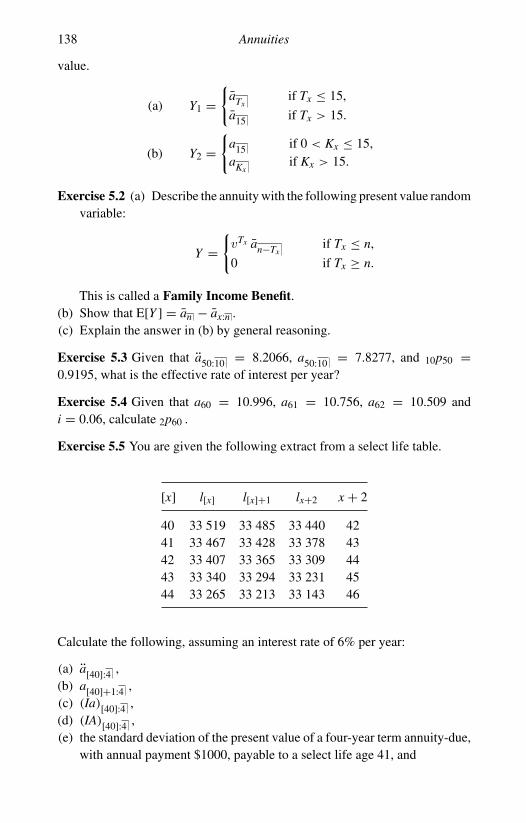
138 Annuities
value.
(a) Y1 ={
aTxif Tx ≤ 15,
a15 if Tx > 15.
(b) Y2 ={
a15 if 0 < Kx ≤ 15,aKx
if Kx > 15.
Exercise 5.2 (a) Describe the annuity with the following present value randomvariable:
Y ={
vTx an−Txif Tx ≤ n,
0 if Tx ≥ n.
This is called a Family Income Benefit.(b) Show that E[Y ] = an − ax:n .(c) Explain the answer in (b) by general reasoning.
Exercise 5.3 Given that a50:10 = 8.2066, a50:10 = 7.8277, and 10p50 =0.9195, what is the effective rate of interest per year?
Exercise 5.4 Given that a60 = 10.996, a61 = 10.756, a62 = 10.509 andi = 0.06, calculate 2p60 .
Exercise 5.5 You are given the following extract from a select life table.
[x] l[x] l[x]+1 lx+2 x + 2
40 33 519 33 485 33 440 4241 33 467 33 428 33 378 4342 33 407 33 365 33 309 4443 33 340 33 294 33 231 4544 33 265 33 213 33 143 46
Calculate the following, assuming an interest rate of 6% per year:
(a) a[40]:4 ,(b) a[40]+1:4 ,(c) (Ia)[40]:4 ,(d) (IA)[40]:4 ,(e) the standard deviation of the present value of a four-year term annuity-due,
with annual payment $1000, payable to a select life age 41, and
5.15 Exercises 139
(f) the probability that the present value of an annuity-due of 1 per year issuedto a select life aged 40 is less than 3.0.
Exercise 5.6 The force of mortality for a certain population is exactly half thesum of the forces of mortality in two standard mortality tables, denoted A and B.Thus
µx = (µAx + µB
x )/2
for all x. A student has suggested the approximation
ax = (aAx + aB
x )/2.
Will this approximation overstate or understate the true value of ax?
Exercise 5.7 Consider a life aged x. Obtain the formula
(IA)x = ax − d(I a)x
by writing down the present value random variables for
(a) an increasing annuity-due to (x) with payments of t + 1 at times t =0, 1, 2, . . . , and
(b) a whole life insurance benefit of amount t at time t, t = 1, 2, 3 . . . , if thedeath of (x) occurs between ages x + t − 1 and x + t.
Hint: use the result
(I a)n =n∑
t=1
tvt−1 = an − nvn
d.
Exercise 5.8 Let H = min(Kx, n).
(a) Show that
V[aH ] =2Ax:n+1 −
(Ax:n+1
)2
d2.
(b) An alternative form given for this variance is
(1 + i)2 [2A 1x:n − (A 1
x:n )2] − 2(1 + i)A 1x:n vn
npx + v2nnpx(1 − npx)
i2.
Prove that this is equal to the expression in (a).

140 Annuities
Exercise 5.9 Consider the random variables Y = aTxand Z = vTx .
(a) Explain briefly why the covariance of Y and Z is negative.(b) Derive an expression for the covariance, in terms of standard actuarial
functions.(c) Show that the covariance is negative.
Exercise 5.10 Find, and simplify where possible:
(a) ddx ax, and
(b) ddx ax:n .
Exercise 5.11 Consider the following portfolio of annuities-due currently beingpaid from the assets of a pension fund.
AgeNumber ofannuitants
60 4070 3080 10
Each annuity has an annual payment of $10 000 as long as the annuitantsurvives. The lives are assumed to be independent. Calculate
(a) the expected present value of the total outgo on annuities,(b) the standard deviation of the present value of the total outgo on annu-
ities, and(c) the 95th percentile of the distribution of the present value of the total outgo
on annuities using a Normal approximation.
Exercise 5.12 Consider the quantities α(m) and β(m) in formula (5.38). Byexpressing i, i(m), d and d (m) in terms of δ, show that
α(m) ≈ 1 and β(m) ≈ m − 1
2m.
Exercise 5.13 Using a spreadsheet, calculate the mean and variance of thepresent value of
(a) an arithmetically increasing term annuity-due payable to a life aged 50for at most 10 years under which the payment at time t is t + 1 for t =0, 1, . . . , 9, and
(b) a geometrically increasing term annuity-due payable to a life aged 50 for atmost 10 years under which the payment at time t is 1.03t for t = 0, 1, . . . , 9.
5.15 Exercises 141
Exercise 5.14 Using a spreadsheet, calculate the mean and variance of thepresent value of
(a) a whole life annuity-due to a life aged 65, with annual payments of 1, and(b) a whole life annuity-due to a life aged 65, with annual payments of 1 and a
guarantee period of 10 years.
Explain the ordering of the means and variances.
Exercise 5.15 Jensen’s inequality states that for a function f , whose firstderivative is positive and whose second derivative is negative, and a randomvariable X ,
E[f (X )] ≤ f (E[X ]) .
Use Jensen’s inequality to show that
ax ≤ aE[Tx] .
Answers to selected exercises
5.3 4.0014%5.4 0.982205.5 (a) 3.66643
(b) 3.45057(c) 8.37502(d) 3.16305(e) 119.14(f) 0.00421
5.11 (a) 10 418 961(b) 311 534(c) 10 931 390
5.13 (a) 40.95, 11.057(b) 9.121, 0.32965
5.14 (a) 13.550, 12.497(b) 13.814, 8.380

6
Premium calculation
6.1 Summary
In this chapter we discuss principles of premium calculation for insurancepolicies and annuities. We start by reviewing what we mean by the terms ‘pre-mium’, ‘net premium’and ‘gross premium’. We next introduce the present valueof future loss random variable. We define the equivalence premium principleand we show how this premium principle can be applied to calculate premiumsfor different types of policy. We look at how we can use the future loss randomvariable to determine when a contract moves from loss to profit or vice versa.We introduce a different premium principle, the portfolio percentile premiumprinciple, and show how, using the mean and variance of the future loss randomvariable, the portfolio percentile premium principle can be used to determinea premium. The chapter concludes with a discussion of how a premium can becalculated when the insured life is subject to some extra level of risk.
6.2 Preliminaries
An insurance policy is a financial agreement between the insurance companyand the policyholder. The insurance company agrees to pay some benefits, forexample a sum insured on the death of the policyholder within the term of aterm insurance, and the policyholder agrees to pay premiums to the insurancecompany to secure these benefits. The premiums will also need to reimbursethe insurance company for the expenses associated with the policy.
The calculation of the premium may not explicitly allow for the insurancecompany’s expenses. In this case we refer to a net premium (also, sometimes, arisk premium or mathematical premium). If the calculation does explicitly allowfor expenses, the premium is called a gross premium or office premium.
The premium may be a single payment by the policyholder – a single pre-mium – or it may be a regular series of payments, possibly annually, quarterly,monthly or weekly. Monthly premiums are very common since many employed
142
6.3 Assumptions 143
people receive their salaries monthly and it is convenient to have payments madewith the same frequency as income is received.
It is common for regular premiums to be a level amount, but they do nothave to be.
A key feature of any life insurance policy is that premiums are payable inadvance, with the first premium payable when the policy is purchased. To seewhy this is necessary, suppose it were possible to purchase a whole life insurancepolicy with annual premiums where the first premium were payable at the endof the year in which the policy was purchased. In this case, a person couldpurchase the policy and then withdraw from the contract at the end of the firstyear before paying the premium then due. This person would have had a yearof insurance cover without paying anything for it.
Regular premiums for a policy on a single life cease to be payable on thedeath of the policyholder. The premium paying term for a policy is the maximumlength of time for which premiums are payable. The premium paying term maybe the same as the term of the policy, but it could be shorter. If we consider awhole life insurance policy, it would be usual for the death benefit to be securedby regular premiums and it would be common for premium payment to ceaseat a certain age – perhaps at age 65 when the policyholder is assumed to retire,or at age 80 when the policyholder’s real income may be diminishing.
As we discussed in Chapter 1, premiums are payable to secure annuity ben-efits as well as life insurance benefits. Deferred annuities may be purchasedusing a single premium at the start of the deferred period, or by regular premi-ums payable throughout the deferred period. Immediate annuities are alwayspurchased by a single premium. For example, a person aged 45 might secure aretirement income by paying regular premiums over a 20-year period to secureannuity payments from age 65. Or, a person aged 65 might secure a monthlyannuity from an insurance company by payment of a single premium.
For traditional policies, the benchmark principle for calculating both grossand net premiums is called the equivalence principle, and we discuss its appli-cation in detail in this chapter. However, there are other methods of calculatingpremiums and we discuss one of these, the portfolio percentile principle.
A more contemporary approach, which is commonly used for non-traditionalpolicies, is to consider the cash flows from the contract, and to set the premiumto satisfy a specified profit criterion. This approach is discussed in Chapter 11.
6.3 Assumptions
As in Chapter 4, unless otherwise stated, we use a standard set of assumptionsfor mortality and interest in the numerical examples in this chapter. We use theselect survival model with a two-year select period specified in Example 3.13

144 Premium calculation
Table 6.1. Annuity values using the Standard Select Survival Model.
x a[x] a[x]+1 ax+2 x + 2 x a[x] a[x]+1 ax+2 x + 2
20 19.96732 19.91993 19.87070 22 51 16.85028 16.66175 16.46782 53
21 19.92062 19.87095 19.81934 23 52 16.66514 16.46908 16.26762 54
22 19.87165 19.81959 19.76549 24 53 16.47277 16.26899 16.05987 55
23 19.82030 19.76574 19.70903 25 54 16.27303 16.06137 15.84443 56
24 19.76647 19.70929 19.64985 26 55 16.06579 15.84608 15.62122 57
25 19.71003 19.65012 19.58783 27 56 15.85091 15.62302 15.39012 58
26 19.65087 19.58810 19.52282 28 57 15.62831 15.39210 15.15109 59
27 19.58887 19.52310 19.45471 29 58 15.39789 15.15325 14.90407 60
28 19.52389 19.45500 19.38336 30 59 15.15960 14.90644 14.64906 61
29 19.45581 19.38365 19.30862 31 60 14.91340 14.65165 14.38606 62
30 19.38449 19.30892 19.23034 32 61 14.65927 14.38890 14.11512 63
31 19.30979 19.23066 19.14838 33 62 14.39724 14.11822 13.83632 64
32 19.23156 19.14871 19.06258 34 63 14.12736 13.83972 13.54979 65
33 19.14965 19.06292 18.97277 35 64 13.84972 13.55351 13.25568 66
34 19.06390 18.97313 18.87880 36 65 13.56444 13.25975 12.95420 67
35 18.97415 18.87917 18.78049 37 66 13.27169 12.95864 12.64561 68
36 18.88024 18.78088 18.67766 38 67 12.97168 12.65045 12.33019 69
37 18.78201 18.67807 18.57014 39 68 12.66467 12.33547 12.00830 70
38 18.67927 18.57058 18.45776 40 69 12.35097 12.01406 11.68035 71
39 18.57184 18.45822 18.34031 41 70 12.03093 11.68661 11.34678 72
40 18.45956 18.34081 18.21763 42 71 11.70495 11.35359 11.00812 73
41 18.34224 18.21815 18.08951 43 72 11.37350 11.01550 10.66491 74
42 18.21969 18.09007 17.95577 44 73 11.03709 10.67291 10.31778 75
43 18.09172 17.95637 17.81621 45 74 10.69629 10.32644 9.96740 76
44 17.95814 17.81686 17.67065 46 75 10.35171 9.97676 9.61449 77
45 17.81876 17.67135 17.51889 47 76 10.00402 9.62458 9.25981 78
46 17.67340 17.51965 17.36074 48 77 9.65395 9.27067 8.90416 79
47 17.52187 17.36156 17.19602 49 78 9.30225 8.91584 8.54841 80
48 17.36397 17.19691 17.02453 50 79 8.94973 8.56093 8.19341 81
49 17.19952 17.02551 16.84612 51 80 8.59722 8.20681 7.84008 82
50 17.02835 16.84718 16.66060 52
with an interest rate of 5% per year effective. Recall that the survival model isspecified as follows:
µx = A + Bcx
where A = 0.00022, B = 2.7 × 10⁻⁶ and c = 1.124. and
µ[x]+s = 0.92−sµx+s
for 0 ≤ s ≤ 2. The select and ultimate life table, at integer ages, for this modelis shown in Table 3.7 and values of Ax at an effective rate of interest of 5%
6.4 The present value of future loss random variable 145
per year are shown in Table 4.1. We refer to this model as the Standard SelectSurvival Model.
Example 6.1 Use the Standard Select Survival Model described above, withinterest at 5% per year, to produce a table showing values of a[x], a[x]+1 andax+2 for x = 20, 21, . . . , 80. Assume that q131 = 1.
Solution 6.1 The calculation of survival probabilities p[x], p[x]+1 and px forthis survival model was discussed in Example 3.13. Since we are assuming thatq131 = 1, we have a131 = 1. Annuity values can then be calculated recursivelyusing
ax = 1 + v px ax+1 ,
a[x]+1 = 1 + v p[x]+1 ax+2 ,
a[x] = 1 + v p[x] a[x]+1 .
Values are shown in Table 6.1. �
6.4 The present value of future loss random variable
The cash flows for a traditional life insurance contract consist of the insurance orannuity benefit outgo (and associated expenses) and the premium income. Bothare generally life contingent, that is, the income and outgo cash flows dependon the future lifetime of the policyholder, unless the contract is purchased by asingle premium, in which case there is no uncertainty regarding the premiumincome. So we can model the future outgo less future income with the randomvariable that represents the present value of the future loss. When expensesare excluded we call this the net future loss, which we denote by Ln
0. Whenexpenses are included, then the premiums are the gross premiums, and therandom variable is referred to as the gross future loss, denoted Lg
0. In otherwords,
Ln0 = PV of benefit outgo − PV of net premium income
Lg0 = PV of benefit outgo + PV of expenses − PV of gross premium income.
In cases where the meaning is obvious from the context, we will drop the n org superscript.
Example 6.2 An insurer issues a whole life insurance to [60], with sum insuredS payable immediately on death. Premiums are payable annually in advance,ceasing at age 80 or on earlier death. The net annual premium is P.

146 Premium calculation
Write down the net future loss random variable, Ln0, for this contract in terms
of lifetime random variables for [60].Solution 6.2 From Chapter 4, we know that the present value random variablefor the benefit is SvT[60] and from Chapter 5 we know that the present valuerandom variable for the premium income is Pamin(K[60]+1,20)
, so
Ln0 = SvT[60] − Pamin(K[60]+1,20)
.
Since both terms of the random variable depend on the future lifetime of thesame life, [60], they are clearly dependent.
Note that since premiums are payable in advance, premiums payable annu-ally in advance, ceasing at age 80 or on earlier death means that the lastpossible premium is payable on the policyholder’s 79th birthday. No premiumis payable on reaching age 80. �
Given an appropriate survival model together with assumptions about futureinterest rates and, for gross premiums, expenses, the insurer can then determinea distribution for the present value of the future loss. This distribution can beused to find a suitable premium for a given benefit, or an appropriate benefitfor a specified premium. To do this, the insurer needs to use a premium prin-ciple. This is a method of selecting an appropriate premium using a given lossdistribution. We discuss two premium principles in this chapter.
6.5 The equivalence principle
6.5.1 Net premiums
For net premiums, we take into consideration outgo on benefit payments only.Thus, expenses are not a part of net premium calculation. The benefit may be adeath benefit or a survival benefit or a combination.
We start by stating the equivalence principle. Under the equivalence principle,the net premium is set such that the expected value of the future loss is zero atthe start of the contract. That means that
E[Ln0] = 0
which implies that
E[PV of benefit outgo − PV of net premium income] = 0.
That is, under the equivalence premium principle,
EPV of benefit outgo = EPV of net premium income. (6.1)

6.5 The equivalence principle 147
The equivalence principle is the most common premium principle in traditionallife insurance, and will be our default principle – that is, if no other principle isspecified, it is assumed that the equivalence principle is to be used.
Example 6.3 Consider an endowment insurance with term n years and suminsured S payable at the earlier of the end of the year of death or at maturity,issued to a select life aged x. Premiums of amount P are payable annuallythroughout the term of the insurance.
Derive expressions in terms of S, P and standard actuarial functions for
(a) the net future loss, Ln0,
(b) the mean of Ln0,
(c) the variance of Ln0, and,
(d) the annual net premium for the contract.
Solution 6.3 (a) The future loss random variable is
Ln0 = Svmin(K[x]+1,n) − Pamin(K[x]+1,n)
.
(b) The mean of Ln0 is
E[Ln0] = SE
[vmin(K[x]+1,n)
]− PE
[amin(K[x]+1,n)
]= SA[x]:n − Pa[x]:n .
(c) Expanding the expression above for Ln0 gives
Ln0 = Svmin(K[x]+1,n) − P
1 − vmin(K[x]+1,n)
d
=(
S + P
d
)vmin(K[x]+1,n) − P
d,
which isolates the random variable vmin(K[x]+1,n). So the variance is
V[Ln
0
] =(
S + P
d
)2
V[vmin(K[x]+1,n)
]
=(
S + P
d
)2 (2A[x]:n − (A[x]:n )2
).
(d) Setting the EPVs of the premiums and benefits to be equal gives the netpremium as
P = SA[x]:na[x]:n
. (6.2)
�

148 Premium calculation
Furthermore, using formula (6.2) and recalling that
ax:n = 1 − Ax:n
d,
we see that the solution can be written as
P = S
(1
a[x]:n− d
)
so that the only actuarial function needed to calculate P for a given value of Sis a[x]:n .
Example 6.4 An insurer issues a regular premium deferred annuity contractto a select life aged x. Premiums are payable monthly throughout the deferredperiod. The annuity benefit of X per year is payable monthly in advance fromage x + n for the remainder of the life of (x).
(a) Write down the net future loss random variable in terms of lifetime randomvariables for [x].
(b) Derive an expression for the monthly net premium.(c) Assume now that, in addition, the contract offers a death benefit of S payable
immediately on death during the deferred period. Write down the net futureloss random variable for the contract, and derive an expression for themonthly net premium.
Solution 6.4 (a) Let P denote the monthly net premium, so that the totalpremium payable in a year is 12P. Then
Ln0 =
⎧⎪⎪⎪⎨⎪⎪⎪⎩
0 − 12Pa(12)
K (12)[x] + 1
12
if T[x] ≤ n,
X vn a(12)
K (12)[x] + 1
12 −n− 12Pa(12)
n if T[x] > n.
(b) The EPV of the annuity benefit is
X vnnp[x] a(12)
[x]+n ,
and the EPV of the premium income is
12Pa(12)
[x]:n .
By equating these EPVs we obtain the premium equation which gives
P = X vnnp[x] a(12)
[x]+n
12a(12)
[x]:n= nE[x] X a(12)
[x]+n
12a(12)
[x]:n.

6.5 The equivalence principle 149
(c) We now have
Ln0 =
⎧⎪⎪⎪⎨⎪⎪⎪⎩
SvT[x] − 12Pa(12)
K (12)[x] + 1
12
if T[x] ≤ n,
X vn a(12)
K (12)[x] + 1
12 −n− 12Pa(12)
n if T[x] > n.
The annuity benefit has the same EPV as in part (b); the death benefitduring deferral is a term insurance benefit with EPV SA1
[x]:n , so the premiumequation now gives
P = SA 1[x]:n + X vn
np[x] a(12)[x]+n
12a(12)
[x]:n.
�
Example 6.4 shows that the future loss random variable can be quite compli-cated to write down. Usually, the premium calculation does not require theidentification of the future loss random variable. We may go directly to theequivalence principle, and equate the EPV of the benefit outgo to the EPV ofthe net premium income to obtain the net premium.
Example 6.5 Consider an endowment insurance with sum insured $100 000issued to a select life aged 45 with term 20 years under which the death benefitis payable at the end of the year of death. Using the Standard Select SurvivalModel, with interest at 5% per year, calculate the total amount of net premiumpayable in a year if premiums are payable (a) annually, (b) quarterly, and (c)monthly, and comment on these values.
Solution 6.5 Let P denote the total amount of premium payable in a year. Thenthe EPV of premium income is Pa(m)
[45]:20(where m = 1, 4 or 12) and the EPV
of benefit outgo is 100 000A[45]:20 , giving
P = 100 000A[45]:20
a(m)
[45]:20
.
Using Tables 3.7 and 6.1, we have
a[45]:20 = a[45] − l65
l[45]v20a[65] = 12.94092.
From this we get
A[45]:20 = 1 − da[45]:20 = 0.383766.
Hence, for m = 1 the net premium is P = $2 965.52.

150 Premium calculation
Table 6.2. Annuity values and premiums.
m = 4 m = 12
Method a(4)
[45]:20P a(12)
[45]:20P
Exact 12.69859 3 022.11 12.64512 3 034.89UDD 12.69839 3 022.16 12.64491 3 034.94W3 12.69859 3 022.11 12.64512 3 034.89
The values of a(m)
[45]:20for m = 4 and 12 can either be calculated exactly
or from a[45]:20 using one of the approximations in Section 5.11. Notice thatthe approximation labelled W3∗ in that section is not available since p[x]−1
is meaningless and so we cannot estimate µ[45] from the life table tabulatedat integer ages. Table 6.2 shows values obtained using the UDD assumptionand Woolhouse’s formula with three terms. The ordering of these premiumsfor m = 1, 4, 12 reflects the ordering of EPVs of 1/mthly annuities which weobserved in Chapter 5. In this example, Woolhouse’s formula provides a verygood approximation, whilst the UDD assumption gives a reasonably accuratepremium.
6.6 Gross premium calculation
When we calculate a gross premium for an insurance policy or an annuity, wetake account of the expenses the insurer incurs. There are three main typesof expense associated with policies – initial expenses, renewal expenses andtermination expenses.
Initial expenses are incurred by the insurer when a policy is issued, and whenwe calculate a gross premium, it is conventional to assume that the insurerincurs these expenses at exactly the same time as the first premium is payable,although in practice these expenses are usually incurred slightly ahead of thisdate. There are two major types of initial expenses – commission to agents forselling a policy and underwriting expenses. Commission is often paid to anagent in the form of a high percentage of the first year’s premiums plus a muchlower percentage of subsequent premiums, payable as the premiums are paid.Underwriting expenses may vary according to the amount of the death benefit.For example, an insurer is likely to require much more stringent medical tests onan individual wanting a $10 million death benefit compared with an individualwanting a $10 000 death benefit.
Renewal expenses are normally incurred by the insurer each time a premiumis payable, and in the case of an annuity, they are normally incurred when an

6.6 Gross premium calculation 151
annuity payment is made. These costs arise in a variety of ways. The processingof renewal and annuity payments involves staff time and investment expenses.Renewal expenses also cover the ongoing fixed costs of the insurer such asstaff salaries and rent for the insurer’s premises, as well as specific costs suchas annual statements to policyholders about their policies.
Initial and renewal expenses may be proportional to premiums, proportionalto benefits or may be ‘per policy’, meaning that the amount is fixed for allpolicies, and is not related to the size of the contract. Often, per policy renewalcosts are assumed to be increasing at a compound rate over the term of thepolicy, to approximate the effect of inflation.
Termination expenses occur when a policy expires, typically on the deathof a policyholder (or annuitant) or on the maturity date of a term insuranceor endowment insurance. Generally these expenses are small, and are largelyassociated with the paperwork required to finalize and pay a claim. In calculatinggross premiums, specific allowance is often not made for termination expenses.Where allowance is made, it is usually proportional to the benefit amount.
In practice, allocating the different expenses involved in running an insurancecompany is a complicated task, and in the examples in this chapter we simplyassume that all expenses are known.
The equivalence principle applied to the gross premiums and benefits statesthat the EPV of the gross future loss random variable should be equal to zero.That means that
E[Lg0] = 0,
that is
EPV of benefit outgo + EPV of expenses
− EPV of gross premium income = 0.
In other words, under the equivalence premium principle,
EPV of benefits + EPV of expenses = EPV of gross premium income.
(6.3)
We conclude this section with three examples in each of which we apply theequivalence principle to calculate gross premiums.
Example 6.6 An insurer issues a 25-year annual premium endowment insur-ance with sum insured $100 000 to a select life aged 30. The insurer incursinitial expenses of $2000 plus 50% of the first premium, and renewal expensesof 2.5% of each subsequent premium. The death benefit is payable immediatelyon death.

152 Premium calculation
(a) Write down the gross future loss random variable.(b) Calculate the gross premium using the Standard Select Survival Model with
5% per year interest.
Solution 6.6 (a) Let S = 100 000, x = 30, n = 25 and let P denote the annualgross premium. Then
Lg0 = S vmin(T[x],n) + 2000 + 0.475P + 0.025Pamin(K[x]+1,n)
− Pamin(K[x]+1,n)
= S vmin(T[x],n) + 2000 + 0.475P − 0.975Pamin(K[x]+1,n).
Note that the premium related expenses, of 50% of the first premium plus2.5% of the second and subsequent premiums are more conveniently writtenas 2.5% of all premiums, plus an additional 47.5% of the first premium.By expressing the premium expenses this way, we can simplify the grossfuture loss random variable, and the subsequent premium calculation.
(b) We may look separately at the three parts of the gross premium equationof value. The EPV of premium income is
Pa[30]:25 = 14.73113 P.
Note that a[30]:25 can be calculated from Tables 3.7 and 6.1.The EPV of all expenses is
2000+0.475P+0.025Pa[30]:25 = 2000 + 0.475P + 0.025 × 14.73113P
= 2000 + 0.843278P.
The EPV of the death benefit can be found using numerical integration orusing Woolhouse’s formula, and we obtain
100 000A[30]:25 = 100 000 × 0.298732 = 29 873.2 .
Thus, the equivalence principle gives
P = 29 873.2 + 2 000
14.73113 − 0.843278= $2 295.04 .
�
Example 6.7 Calculate the monthly gross premium for a 10-year term insurancewith sum insured $50 000 payable immediately on death, issued to a select life
6.6 Gross premium calculation 153
aged 55, using the following basis:
Survival model: Standard Select Survival ModelAssume UDD for fractional ages
Interest: 5% per yearInitial Expenses: $500 +10% of each monthly premium in the first yearRenewal Expenses: 1% of each monthly premium in the second and
subsequent policy years
Solution 6.7 Let P denote the monthly premium. Then the EPV of premiumincome is 12Pa(12)
[55]:10. To find the EPV of premium related expenses, we can
apply the same idea as in the previous example, noting that initial expensesapply to each premium in the first year. Thus, we can write the EPV of allexpenses as
500 + 0.09 × 12Pa(12)
[55]:1 + 0.01 × 12Pa(12)
[55]:10
where the expenses for the first year have been split as 9% plus 1%, so that wehave 9% in the first year and 1% every year. The EPV of the insurance benefitis 50 000A 1
[55]:10and so the equivalence principle gives
12P(
0.99a(12)
[55]:10− 0.09a(12)
[55]:1)
= 500 + 50 000A 1[55]:10
.
We find that a(12)
[55]:10= 7.8341, a(12)
[55]:1 = 0.9773 and A 1[55]:10
= 0.024954,
giving P = $18.99 per month.Calculating all the EPVs exactly gives the same answer for the premium to
four significant figures. �
Example 6.8 Calculate the gross single premium for a deferred annuity of$80 000 per year payable monthly in advance, issued to a select life now aged50 with the first annuity payment on the life’s 65th birthday. Allow for initialexpenses of $1 000, and renewal expenses on each anniversary of the issue date,provided that the policyholder is alive. Assume that the renewal expense willbe $20 on the first anniversary of the issue date, and that expenses will increasewith inflation from that date at the compound rate of 1% per year. Assume theStandard Select Survival Model with interest at 5% per year.
Solution 6.8 The single premium is equal to the EPV of the deferred annuityplus the EPV of expenses. The renewal expense on the tth policy anniversary

154 Premium calculation
is 20(1.01t−1
)for t = 1, 2, 3, . . . so that the EPV of renewal expenses is
20∞∑
t=1
1.01t−1 vttp[50] = 20
1.01
∞∑t=1
1.01t vttp[50]
= 20
1.01
∞∑t=1
vtj tp[50]
= 20
1.01(a[50] j − 1)
where the subscript j indicates that the calculation is at rate of interest j where1.01v = 1/(1 + j), that is j = 0.0396. The EPV of the deferred annuity is80 000 15|a(12)
[50] , so the single premium is
1 000 + 20
1.01(a[50] j − 1) + 80 000 15|a(12)
[50] .
As a[50] j = 19.4550 and 15|a(12)[50] = 6.04129, the single premium is $484 669.
�
We end this section with a comment on the premiums calculated in Examples6.6 and 6.7. In Example 6.6, the annual premium is $2295.04 and the expensesat time 0 are $2 000 plus 50% of the first premium, a total of $3146.75, whichexceeds the first premium. Similarly, in Example 6.7 the total premium in thefirst year is $227.88 and the total expenses in the first year are $500 plus 10%of premiums in the first year. In each case, the premium income in the first yearis insufficient to cover expenses in the first year. This situation is common inpractice, especially when initial commission to agents is high, and is referredto as new business strain. A consequence of new business strain is that aninsurer needs to have funds available in order to sell policies. From time to timeinsurers get into financial difficulties through pursuing an aggressive growthstrategy without sufficient capital to support the new business strain. Essentially,the insurer borrows from shareholder (or participating policyholder) funds inorder to write new business. These early expenses are gradually paid off by theexpense loadings in future premiums. The part of the premiums that funds theinitial expenses is called the deferred acquisition cost.
6.7 Profit
The equivalence principle does not allow explicitly for a loading for profit. Sincewriting business generally involves a loan from shareholder or participating

6.7 Profit 155
policyholder funds, it is necessary for the business to be sufficiently profitablefor the payment of a reasonable rate of return – in other words, to make aprofit. In traditional insurance, we often load for profit implicitly, by marginsin the valuation assumptions. For example, if we expect to earn an interest rateof 6% per year on assets, we might assume only 5% per year in the premiumbasis. The extra income from the invested premiums will contribute to profit. Inparticipating business, much of the profit will be distributed to the policyholdersin the form of cash dividends or bonus. Some will be paid as dividends toshareholders, if the company is proprietary.
We may also use margins in the mortality assumptions. For a term insurance,we might use a slightly higher overall mortality rate than we expect. For anannuity, we might use a slightly lower rate.
More modern premium setting approaches, which use projected cash flows,are presented in Chapter 11, where more explicit allowance for profit isincorporated in the methodology.
Each individual policy sold will generate a profit or a loss.Although we calcu-late a premium assuming a given survival model, for each individual policy theexperienced mortality rate in any year can take only the values 0 or 1. So, whilethe expected outcome under the equivalence principle is zero profit (assumingno margins), the actual outcome for each individual policy will either be a profitor a loss. For the actual profit from a group of policies to be reliably close to theexpected profit, we need to sell a large number of individual contracts, whosefuture lifetimes can be regarded as statistically independent, so that the lossesand profits from individual policies are combined.
As a simple illustration of this, consider a life who purchases a one-year terminsurance with sum insured $1000 payable at the end of the year of death. Letus suppose that the life is subject to a mortality of rate of 0.01 over the year,that the insurer can earn interest at 5% per year, and that there are no expenses.Then, using the equivalence principle, the premium is
P = 1 000 × 0.01/1.05 = 9.52.
The future loss random variable is
Ln0 =
{1 000v − P = 942.86 if Tx ≤ 1, with probability 0.01,−P = −9.52 if Tx > 1, with probability 0.99.
The expected loss is 0.01 × 942.86 + 0.99 × (−9.52) = 0, as required by theequivalence principle, but the probability of profit is 0.99, and the probability ofloss is 0.01. The balance arises because the profit, if the policyholder survives

156 Premium calculation
the year, is small, and the loss, if the policyholder dies, is large. Using theequivalence principle, so that the expected future loss is zero, makes sense onlyif the insurer issues a large number of policies, so that the overall proportion ofpolicies becoming claims will be close to the assumed proportion of 0.01.
Now suppose the insurer were to issue 100 such policies to independent lives.The insurer would expect to make a (small) profit on 99 of them. If the outcomefrom this portfolio is that all lives survive for the year, then the insurer makesa profit. If one life dies, there is no profit or loss. If more than one life dies,there will be a loss on the portfolio. Let D denote the number of deaths in theportfolio, so that D ∼ B(100, 0.01). The probability that the profit on the wholeportfolio is greater than or equal to zero is
Pr[D ≤ 1] = 0.73576
compared with 99% for the individual contract. In fact, as the number of policiesissued increases, the probability of profit will tend, monotonically, to 0.5. Onthe other hand, while the probability of loss is increasing with the portfolio size,the probability of very large aggregate losses (relative, say, to total premiums)is much smaller for a large portfolio, since there is a balancing effect fromdiversification of the risk amongst the large group of policies.
Let us now consider a whole life insurance policy with sum insured S payableat the end of the year of death, initial expenses of I , renewal expenses of eassociated with each premium payment (including the first) issued to a selectlife aged x by annual premiums of P. For this policy
Lg0 = SvK[x]+1 + I + e aK[x]+1 − P aK[x]+1 ,
where K[x] denotes the curtate future lifetime of [x].If death occurs shortly after the policy is issued, so that only a few premiums
are paid, the insurer will make a loss, and, conversely, if the policyholder livesto a ripe old age, we would expect that the insurer would make a profit asthe policyholder will have paid a large number of premiums, and there willhave been plenty of time for the premiums to accumulate interest. We canuse the future loss random variable to find the minimum future lifetime forthe policyholder in order that the insurer makes a profit on this policy. Theprobability that the insurer makes a profit on the policy, Pr[Lg
0 < 0], is given by
Pr[Lg0 < 0] = Pr
[SvK[x]+1 + I + e aK[x]+1 − P aK[x]+1 < 0
].
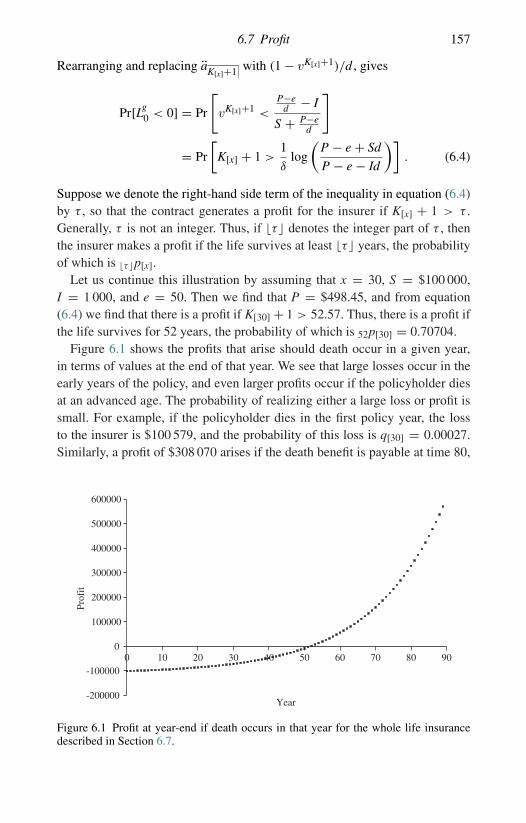
6.7 Profit 157
Rearranging and replacing aK[x]+1 with (1 − vK[x]+1)/d , gives
Pr[Lg0 < 0] = Pr
[vK[x]+1 <
P−ed − I
S + P−ed
]
= Pr
[K[x] + 1 >
1
δlog
(P − e + Sd
P − e − Id
)]. (6.4)
Suppose we denote the right-hand side term of the inequality in equation (6.4)by τ , so that the contract generates a profit for the insurer if K[x] + 1 > τ .Generally, τ is not an integer. Thus, if �τ denotes the integer part of τ , thenthe insurer makes a profit if the life survives at least �τ years, the probabilityof which is �τp[x].
Let us continue this illustration by assuming that x = 30, S = $100 000,I = 1 000, and e = 50. Then we find that P = $498.45, and from equation(6.4) we find that there is a profit if K[30] + 1 > 52.57. Thus, there is a profit ifthe life survives for 52 years, the probability of which is 52p[30] = 0.70704.
Figure 6.1 shows the profits that arise should death occur in a given year,in terms of values at the end of that year. We see that large losses occur in theearly years of the policy, and even larger profits occur if the policyholder diesat an advanced age. The probability of realizing either a large loss or profit issmall. For example, if the policyholder dies in the first policy year, the lossto the insurer is $100 579, and the probability of this loss is q[30] = 0.00027.Similarly, a profit of $308 070 arises if the death benefit is payable at time 80,
-200000
-100000
0
100000
200000
300000
400000
500000
600000
0 10 20 30 40 50 60 70 80 90
Year
Prof
it
Figure 6.1 Profit at year-end if death occurs in that year for the whole life insurancedescribed in Section 6.7.

158 Premium calculation
and the probability of this is 79|q[30] = 0.00023. It is important to appreciatethat the premium has been calculated in such a way that the EPV of the profitfrom the policy is zero.
Example 6.9 A life insurer is about to issue a 25-year endowment insurancewith a basic sum insured of $250 000 to a select life aged exactly 30. Premiumsare payable annually throughout the term of the policy. Initial expenses are$1200 plus 40% of the first premium and renewal expenses are 1% of the secondand subsequent premiums. The insurer allows for a compound reversionarybonus of 2.5% of the basic sum insured, vesting on each policy anniversary(including the last). The death benefit is payable at the end of the year of death.Assume the Standard Select Survival Model with interest at 5% per year.
(a) Derive an expression for the future loss random variable, Lg0, for this policy.
(b) Calculate the annual premium for this policy.(c) Let L0(k) denote the present value of the loss on the policy given that
K[30] = k for k ≤ 24 and let L0(25) denote the present value of the loss onthe policy given that the policyholder survives to age 55. Calculate L0(k)
for k = 0, 1, . . . , 25.(d) Calculate the probability that the insurer makes a profit on this policy.(e) Calculate V[Lg
0].Solution 6.9 (a) First, we note that if the policyholder’s curtate future lifetime,
K[30], is k years where k = 0, 1, 2, . . . , 24, then the number of bonus addi-tions is k, the death benefit is payable k +1 years from issue, and hence thepresent value of the death benefit is 250 000(1.025)K[30]vK[30]+1. However,if the policyholder survives for 25 years, then 25 bonuses vest. Thus, if Pdenotes the annual premium,
Lg0 = 250 000(1.025min(K[30], 25))vmin(K[30]+1, 25)
+ 1 200 + 0.39P − 0.99Pamin(K[30]+1, 25).
(b) The EPV of the premiums, less premium expenses, is
0.99Pa[30]:25 = 14.5838P.
As the death benefit is $250 000(1.025t) if the policyholder dies in the tthpolicy year, the EPV of the death benefit is
250 00024∑
t=0
vt+1t |q[30] (1.025t) = 250 000
(1
1.025A 1
[30]:25 j
)= 3099.37
where 1 + j = (1 + i)/(1.025), so that j = 0.02439.
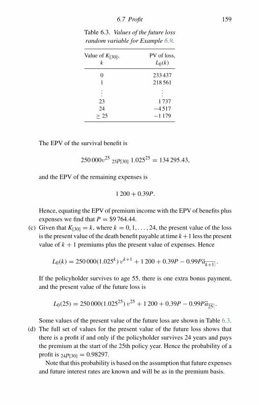
6.7 Profit 159
Table 6.3. Values of the future lossrandom variable for Example 6.9.
Value of K[30],k
PV of loss,L0(k)
0 233 4371 218 561...
...23 1 73724 −4 517
≥ 25 −1 179
The EPV of the survival benefit is
250 000v2525p[30] 1.02525 = 134 295.43,
and the EPV of the remaining expenses is
1 200 + 0.39P.
Hence, equating the EPV of premium income with the EPV of benefits plusexpenses we find that P = $9 764.44.
(c) Given that K[30] = k, where k = 0, 1, . . . , 24, the present value of the lossis the present value of the death benefit payable at time k +1 less the presentvalue of k + 1 premiums plus the present value of expenses. Hence
L0(k) = 250 000(1.025k) vk+1 + 1 200 + 0.39P − 0.99Pak+1 .
If the policyholder survives to age 55, there is one extra bonus payment,and the present value of the future loss is
L0(25) = 250 000(1.02525) v25 + 1 200 + 0.39P − 0.99Pa25 .
Some values of the present value of the future loss are shown in Table 6.3.(d) The full set of values for the present value of the future loss shows that
there is a profit if and only if the policyholder survives 24 years and paysthe premium at the start of the 25th policy year. Hence the probability of aprofit is 24p[30] = 0.98297.
Note that this probability is based on the assumption that future expensesand future interest rates are known and will be as in the premium basis.
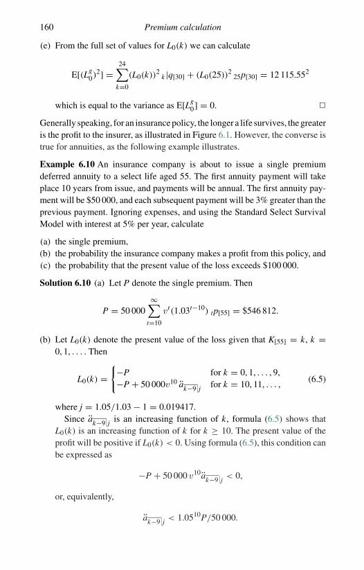
160 Premium calculation
(e) From the full set of values for L0(k) we can calculate
E[(Lg0)2] =
24∑k=0
(L0(k))2k |q[30] + (L0(25))2
25p[30] = 12 115.552
which is equal to the variance as E[Lg0] = 0. �
Generally speaking, for an insurance policy, the longer a life survives, the greateris the profit to the insurer, as illustrated in Figure 6.1. However, the converse istrue for annuities, as the following example illustrates.
Example 6.10 An insurance company is about to issue a single premiumdeferred annuity to a select life aged 55. The first annuity payment will takeplace 10 years from issue, and payments will be annual. The first annuity pay-ment will be $50 000, and each subsequent payment will be 3% greater than theprevious payment. Ignoring expenses, and using the Standard Select SurvivalModel with interest at 5% per year, calculate
(a) the single premium,(b) the probability the insurance company makes a profit from this policy, and(c) the probability that the present value of the loss exceeds $100 000.
Solution 6.10 (a) Let P denote the single premium. Then
P = 50 000∞∑
t=10
vt(1.03t−10) tp[55] = $546 812.
(b) Let L0(k) denote the present value of the loss given that K[55] = k, k =0, 1, . . . . Then
L0(k) ={
−P for k = 0, 1, . . . , 9,−P + 50 000v10 ak−9 j for k = 10, 11, . . . ,
(6.5)
where j = 1.05/1.03 − 1 = 0.019417.Since ak−9 j is an increasing function of k, formula (6.5) shows that
L0(k) is an increasing function of k for k ≥ 10. The present value of theprofit will be positive if L0(k) < 0. Using formula (6.5), this condition canbe expressed as
−P + 50 000 v10ak−9 j < 0,
or, equivalently,
ak−9 j < 1.0510P/50 000.
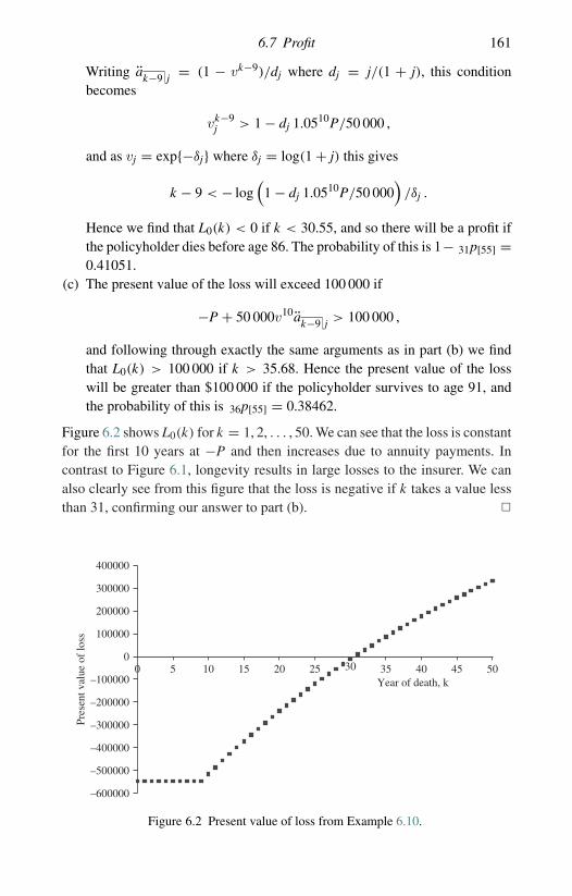
6.7 Profit 161
Writing ak−9 j = (1 − vk−9)/dj where dj = j/(1 + j), this conditionbecomes
vk−9j > 1 − dj 1.0510P/50 000 ,
and as vj = exp{−δj} where δj = log(1 + j) this gives
k − 9 < − log(
1 − dj 1.0510P/50 000)
/δj .
Hence we find that L0(k) < 0 if k < 30.55, and so there will be a profit ifthe policyholder dies before age 86. The probability of this is 1− 31p[55] =0.41051.
(c) The present value of the loss will exceed 100 000 if
−P + 50 000v10ak−9 j > 100 000 ,
and following through exactly the same arguments as in part (b) we findthat L0(k) > 100 000 if k > 35.68. Hence the present value of the losswill be greater than $100 000 if the policyholder survives to age 91, andthe probability of this is 36p[55] = 0.38462.
Figure 6.2 shows L0(k) for k = 1, 2, . . . , 50. We can see that the loss is constantfor the first 10 years at −P and then increases due to annuity payments. Incontrast to Figure 6.1, longevity results in large losses to the insurer. We canalso clearly see from this figure that the loss is negative if k takes a value lessthan 31, confirming our answer to part (b). �
–600000
–500000
–400000
–300000
–200000
–100000
0
100000
200000
300000
400000
0 5 10 15 20 25 30 35 40 45 50Year of death, k
Pres
ent v
alue
of
loss
Figure 6.2 Present value of loss from Example 6.10.
162 Premium calculation
6.8 The portfolio percentile premium principle
The portfolio percentile premium principle is an alternative to the equivalencepremium principle. We assume a large portfolio of identical and independentpolicies. By ‘identical’we mean that the policies have the same premium, bene-fits, term, and so on, and that the policyholders are all subject to the same survivalmodel. By ‘independent’ we mean that the policyholders are independent ofeach other with respect to mortality.
Suppose we know the sum insured for these policies, and wish to find anappropriate premium. As the policies are identical, each policy has the samefuture loss random variable. Let N denote the number of policies in the portfolioand let L0,i represent the future loss random variable for the ith policy in theportfolio, i = 1, 2, 3, . . . , N . The total future loss in the portfolio is L, say, where
L =N∑
i=1
L0,i ; E[L] =N∑
i=1
E[L0,i] = NE[L0,1];
V[L] =N∑
i=1
V[L0,i] = NV[L0,1].
(Note that as {L0,i}Ni=1 are identically distributed, the mean and variance of each
L0,i are equal to the mean and variance of L0,1.)The portfolio percentile premium principle sets a premium so that there is a
specified probability, say α, that the total future loss is negative. That is, P isset such that
Pr[L < 0] = α.
Now, if N is sufficiently large (say, greater than around 30), the central limittheorem tells us that L is approximately normally distributed, with mean E[L] =NE[L0,1] and variance V[L] = NV[L0,1]. In this case, the portfolio percentileprinciple premium can be calculated from
Pr[L < 0] = Pr
(L − E[L]√
V[L] <−E[L]√
V[L])
= �
(−E[L]√V[L]
)= α ,
which implies that
E[L]√V[L] = −�−1(α)
where � is the cumulative distribution function of the standard normaldistribution.
6.8 The portfolio percentile premium principle 163
Our aim is to calculate P, but P does not appear explicitly in either of thelast two equations. However, as illustrated in the next example, both the meanand variance of L are functions of P.
Example 6.11 An insurer issues whole life insurance policies to select livesaged 30. The sum insured of $100 000 is paid at the end of the month of deathand level monthly premiums are payable throughout the term of the policy.Initial expenses, incurred at the issue of the policy, are 15% of the total of thefirst year’s premiums. Renewal expenses are 4% of every premium, includingthose in the first year.
Assume the Standard Select Survival Model with interest at 5% per year.
(a) Calculate the monthly premium using the equivalence principle.(b) Calculate the monthly premium using the portfolio percentile principle,
such that the probability that the future loss on the portfolio is negative is95%. Assume a portfolio of 10 000 identical, independent policies.
Solution 6.11 (a) Let P be the monthly premium. Then the EPV of premiums is
12P a(12)[30] = 227.065P.
The EPV of benefits is
100 000A(12)[30] = 7 866.18,
and the EPV of expenses is
0.15 × 12P + 0.04 × 12P a(12)[30] = 10.8826P.
Equating the EPV of premiums with the EPVs of benefits and expensesgives the equivalence principle premium as $36.39 per month.
(b) The future loss random variable for the ith policy is
L0,i = 100 000vK (12)[30] + 1
12 + 0.15 × 12P − 0.96 × 12P a(12)
K (12)[30] + 1
12
.
and its expected value can be calculated using the solution to part (a) as
E[L0,i] = 7 866.14 − 216.18P.
To find V[L0,i] we can rewrite L0,i as
L0,i =(
100 000 + 0.96 × 12P
d (12)
)vK (12)
[30] + 112 + 0.15 × 12P − 0.96 × 12P
d (12)

164 Premium calculation
so that
V[L0,i] =(
100 000 + 0.96 × 12P
d (12)
)2 (2A(12)
[30] − (A(12)[30])
2)
= (100 000 + 236.59P)2 (0.0053515)
giving √V[L0,i] = (100 000 + 236.59P) (0.073154).
The future loss random variable for the portfolio of policies is L =∑10 000i=1 L0,i, so
E[L] = 10 000(7866.18 − 216.18P)
and
V[L] = 10 000 (100 000 + 236.59P)2 (0.0053515).
Using the normal approximation to the distribution of L, we set P such that
Pr[L < 0] = �
(−E[L]√V[L]
)= �
(10 000(216.18P − 7 866.18)
100 (100 000 + 236.59P) (0.073154)
)
= 0.95.
For the standard normal distribution, �(1.645) = 0.95, so we set
100(216.18P − 7 866.18)
(100 000 + 236.59P) (0.073154)= 1.645
which gives P = $36.99.�
Note that the solution to part (b) above depends on the number of policies inthe portfolio (10 000) and the level of probability we set for the future lossbeing negative (0.95). If the portfolio had n policies instead of 10 000, then theequation we would have to solve for the premium, P, is
√n(216.18P − 7 866.18)
(100 000 + 236.59P) (0.073154)= 1.645. (6.6)
Table 6.4 shows some values of P for different values of n. We note that Pdecreases as n increases. In fact, as n → ∞, P → $36.39, which is theequivalence principle premium. The reason for this is that as n → ∞ theinsurer diversifies the mortality risk. We discuss diversification of risk furtherin Chapter 10.

6.9 Extra risks 165
Table 6.4. Premiumsaccording to portfolio size.
n P
1 000 38.312 000 37.745 000 37.24
10 000 36.9920 000 36.81
6.9 Extra risks
As we discussed in Section 1.3.5, when an individual wishes to effect a lifeinsurance policy, underwriting takes place. If underwriting determines that anindividual should not be offered insurance at standard rates, the individual mightstill be offered insurance, but above standard rates. There are different ways inwhich we can model the extra mortality risk in a premium calculation.
6.9.1 Age rating
One reason why an individual might not be offered insurance at standard ratesis that the individual suffers from a medical condition. In such circumstanceswe refer to the individual as an impaired life, and the insurer may compensatefor this extra risk by treating the individual as being older. For example, animpaired life aged 40 might be asked to pay the same premium paid by a non-impaired life aged 45. This approach to modelling extra risk involves no newideas in premium calculation – for example, we could apply the equivalenceprinciple in our calculation, and we would simply change the policyholder’sage. This is referred to as age rating.
6.9.2 Constant addition to µx
Individuals can also be deemed to be ineligible for standard rates if they reg-ularly participate in hazardous pursuits, for example parachuting. For suchindividuals the extra risk is largely independent of age, and so we could modelthis extra risk by adding a constant to the force of mortality – just as Makehamextended Gompertz’ law of mortality. The application of this approach leads tosome computational shortcuts for the following reason. We are modelling theforce of mortality as
µ′[x]+s = µ[x]+s + φ

166 Premium calculation
where functions with the superscript ′ relate to the impaired life, functionswithout this superscript relate to a standard survival model and φ is the constantaddition to the force of mortality. Then
tp′[x] = exp
{−∫ t
0µ′[x]+sds
}= exp
{−∫ t
0
(µ[x]+s + φ
)ds
}= e−φt
tp[x] .
This formula is useful for computing the EPV of a survival benefit since
e−δttp
′[x] = e−(δ+φ)ttp[x],
so that, for example,
a′[x]:n =
n−1∑t=0
e−δttp
′[x] =n−1∑t=0
e−(δ+φ)ttp[x] = a[x]:n j , (6.7)
where j denotes calculation at interest rate j = eφ+δ − 1. Note that a[x]:n j iscalculated using rate of interest j and the standard survival model.
Now suppose that the impaired life has curtate future lifetime K ′[x]. We knowthat
a′[x]:n = E
[a
min(K ′[x]+1,n)
]= 1 − E[vmin(K ′[x]+1,n)]
d= 1 − A′
[x]:nd
.
So
A′[x]:n = 1 − d a′
[x]:n = 1 − d a[x]:n j . (6.8)
It is important to note here that for the insurance benefit we cannot just changethe interest rate. In formula (6.8), the annuity is evaluated at rate j, but thefunction d uses the original rate of interest, that is d = i/(1 + i). Generally,when using the constant addition to the force of mortality, it is simplest tocalculate the annuity function first, using a simple adjustment of interest, thenuse formula (6.8) for any insurance factors. Note that the standard discountfunction nEx = vn
npx is a survival benefit value, and so can be calculated forthe extra risk by an interest adjustment, so that
nE′x = vn
j npx .
Example 6.12 Calculate the annual premium for a 20-year endowment insur-ance with sum insured $200 000 issued to a life aged 30 whose force of mortalityat age 30 + s is given by µ[30]+s + 0.01. Allow for initial expenses of $2000plus 40% of the first premium, and renewal expenses of 2% of the second and
6.9 Extra risks 167
subsequent premiums. Use the Standard Select Survival Model with interest at5% per year.
Solution 6.12 Let P denote the annual premium. Then by applying formula(6.7), the EPV of premium income is
P19∑
t=0
vttp
′[30] = Pa[30]:20 j
where j = 1.05e0.01 − 1 = 0.06055. Similarly, the EPV of expenses is
2000 + 0.38P + 0.02Pa[30]:20 j .
The EPV of the benefit is 200 000A′[30]:20
, where the dash denotes extra
mortality and the interest rate is i = 0.05. Using formula (6.8)
A′[30]:20
= 1 − d a[30]:20 j .
As a[30]:20 j = 12.072 and d = 0.05/1.05, we find that A′[30]:20
= 0.425158
and hence we find that P = $7 600.84.
6.9.3 Constant multiple of mortality rates
A third method of allowing for extra mortality is to assume that lives are subjectto mortality rates that are higher than the standard lives’ mortality rates. Forexample, we might set q′[x]+t = 1.1q[x]+t where the superscript ′ again denotesextra mortality risk. With such an approach we can calculate the probability ofsurviving one year from any integer age, and hence we can calculate the prob-ability of surviving an integer number of years. A computational disadvantageof this approach is that we have to apply approximations in calculating EPVsif payments are at other than annual intervals. Generally, this form of extra riskwould be handled by recalculating the required functions in a spreadsheet.
Example 6.13 Calculate the monthly premium for a 10-year term insurancewith sum insured $100 000 payable immediately on death, issued to a life aged50. Assume that each year throughout the 10-year term the life is subject tomortality rates that are 10% higher than for a standard life of the same age.Allow for initial expenses of $1000 plus 50% of the first monthly premium andrenewal expenses of 3% of the second and subsequent monthly premiums. Usethe UDD assumption where appropriate, and use the Standard Select SurvivalModel with interest at 5% per year.
168 Premium calculation
Solution 6.13 Let P denote the total premium per year. Then the EPV ofpremium income is Pa(12) ′
50:10and, assuming UDD, we compute a(12) ′
50:10as
a(12) ′50:10
= α(12)a′50:10
− β(12)(
1 − v1010p′
50
),
where
α(12) = id
i(12)d (12)= 1.0002
and
β(12) = i − i(12)
i(12)d (12)= 0.4665.
As the initial expenses are 1000 plus 50% of the first premium, which is 112 P,
we can write the EPV of expenses as
1000 + 0.47P
12+ 0.03Pa(12) ′
50:10.
Finally, the EPV of the death benefit is 100 000(A 150:10
)′ and, using UDD, we
can compute this as
(A 150:10
)′ = i
δ(A 1
50:10)′
= i
δ
((A50:10 )′ − v10
10p′50
)
= i
δ
(1 − da′
50:10− v10
10p′50
).
The formula for a′50:10
is
a′50:10
=9∑
t=0
vttp
′50
where
tp′50 =
t−1∏r=0
(1 − 1.1q[50]+r) . (6.9)
(We have written q[50]+r in formula (6.9) as standard lives are subject to selectmortality.) Hence a′
50:10= 8.0516, a(12) ′
50:10= 7.8669 and (A 1
50:10)′ = 0.01621,
which give P = $345.18 and so the monthly premium is $28.76.

6.10 Notes and further reading 169
Table 6.5. Spreadsheet calculations for Example 6.13.
(1)t
(2)tp′
50
(3)t |q′
50
(4)vt
(5)vt+1
(6)(2) × (4)
(7)(3) × (5)
0 1.0000 0.0011 1.0000 0.9524 1.0000 0.00111 0.9989 0.0014 0.9524 0.9070 0.9513 0.00132 0.9975 0.0016 0.9070 0.8638 0.9047 0.00143 0.9959 0.0018 0.8638 0.8227 0.8603 0.00154 0.9941 0.0020 0.8227 0.7835 0.8178 0.00155 0.9921 0.0022 0.7835 0.7462 0.7774 0.00166 0.9899 0.0024 0.7462 0.7107 0.7387 0.00177 0.9875 0.0027 0.7107 0.6768 0.7018 0.00188 0.9849 0.0030 0.6768 0.6446 0.6666 0.00199 0.9819 0.0033 0.6446 0.6139 0.6329 0.0020
Total 8.0516 0.0158
Table 6.5 shows how we could set out a spreadsheet to perform calculations.Column (2) was created from the original mortality rates using formula (6.9),with column (3) being calculated as
t |q′50 = tp
′50 (1 − 1.1q50+t) .
The total in column (6) gives a ′50:10
while the total in column (7) gives
the value for(
A 150:10
)′.(
Note that this must then by multiplied by i/δ to get(A 1
50:10
)′.
)�
6.10 Notes and further reading
The equivalence principle is the traditional approach to premium calculation,and we apply it again in Chapter 7 when we consider the possibility that apolicy may terminate for reasons other than death. However, other approachesto premium calculation are possible. We have seen one in Section 6.8, wherewe computed premiums by the portfolio percentile principle.
A modification of the equivalence principle which builds an element of profitinto a premium calculation is to select a profit target amount for each policy,, say, and set the premium to be the smallest possible such that E[L0] ≤ .Under this method of calculation we effectively set a level for the expectedpresent value of future profit from the policy and calculate the premium bytreating this amount as an additional cost at the issue date which will be met byfuture premium income.
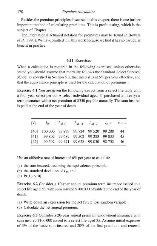
170 Premium calculation
Besides the premium principles discussed in this chapter, there is one furtherimportant method of calculating premiums. This is profit testing, which is thesubject of Chapter 11.
The international actuarial notation for premiums may be found in Bowerset al. (1997). We have omitted it in this work because we find it has no particularbenefit in practice.
6.11 Exercises
When a calculation is required in the following exercises, unless otherwisestated you should assume that mortality follows the Standard Select SurvivalModel as specified in Section 6.3, that interest is at 5% per year effective, andthat the equivalence principle is used for the calculation of premiums.
Exercise 6.1 You are given the following extract from a select life table witha four-year select period. A select individual aged 41 purchased a three-yearterm insurance with a net premium of $350 payable annually. The sum insuredis paid at the end of the year of death.
[x] l[x] l[x]+1 l[x]+2 l[x]+3 lx+4 x + 4
[40] 100 000 99 899 99 724 99 520 99 288 44[41] 99 802 99 689 99 502 99 283 99 033 45[42] 99 597 99 471 99 628 99 030 98 752 46
Use an effective rate of interest of 6% per year to calculate
(a) the sum insured, assuming the equivalence principle,(b) the standard deviation of L0, and(c) Pr[L0 > 0].Exercise 6.2 Consider a 10-year annual premium term insurance issued to aselect life aged 50, with sum insured $100 000 payable at the end of the year ofdeath.
(a) Write down an expression for the net future loss random variable.(b) Calculate the net annual premium.
Exercise 6.3 Consider a 20-year annual premium endowment insurance withsum insured $100 000 issued to a select life aged 35. Assume initial expensesof 3% of the basic sum insured and 20% of the first premium, and renewal

6.11 Exercises 171
expenses of 3% of the second and subsequent premiums. Assume that the deathbenefit is payable at the end of the year of death.
(a) Write down an expression for the gross future loss random variable.(b) Calculate the gross annual premium.(c) Calculate the standard deviation of the gross future loss random variable.(d) Calculate the probability that the contract makes a profit.
Exercise 6.4 Consider an annual premium with-profit whole life insuranceissued to a select life aged exactly 40. The basic sum insured is $200 000 payableat the end of the month of death, and the premium term is 25 years. Assume acompound reversionary bonus of 1.5% per year, vesting on each policy anniver-sary, initial expenses of 60% of the annual premium, renewal expenses of 2.5%of all premiums after the first, plus per policy expenses (incurred when a pre-mium is payable) of $5 at the beginning of the first year, increasing by 6% peryear compound at the beginning of each subsequent year.
Calculate the annual premium.
Exercise 6.5 A select life aged exactly 40 has purchased a deferred annuitypolicy. Under the terms of the policy, the annuity payments will commence 20years from the issue date and will be payable at annual intervals thereafter. Theinitial annuity payment will be $50 000, and each subsequent payment will be2% greater than the previous one. The policy has monthly premiums, payablefor at most 20 years. Calculate the gross monthly premium allowing for initialexpenses of 2.5% of the first annuity payment and 20% of the first premium,renewal expenses of 5% of the second and subsequent premiums, and terminalexpenses, incurred at the end of the year of death, of $20 inflated from the issuedate assuming an inflation rate of 3% per year.
Exercise 6.6 Find the annual premium for a 20-year term insurance with suminsured $100 000 payable at the end of the year of death, issued to a select lifeaged 40 with premiums payable for at most 10 years, with expenses, which areincurred at the beginning of each policy year, as follows:
Year 1 Years 2+
% of premium Constant % of premium Constant
Taxes 4% 0 4% 0Sales commission 25% 0 5% 0Policy maintenance 0% 10 0% 5

172 Premium calculation
Exercise 6.7 A life insurer is about to issue a 30-year deferred annuity-due withannual payments of $20 000 to a select life aged 35. The policy has a singlepremium which is refunded without interest at the end of the year of death ifdeath occurs during the deferred period.
(a) Calculate the single premium for this annuity.(b) The insurer offers an option that if the policyholder dies before the total
annuity payments exceed the single premium, then the balance will be paidas a death benefit, at the end of the year of death. Calculate the revisedpremium.This is called a Cash Refund Payout Option.
Exercise 6.8 A whole life insurance with unit sum insured payable at the endof the year of death with a level annual premium is issued to (x). Let L0 be thenet future loss random variable with the premium determined by the equiva-lence principle. Let L∗
0 be the net future loss random variable if the premium isdetermined such that E[L∗
0] = −0.5.Given V[L0] = 0.75, calculate V[L∗
0].
Exercise 6.9 Calculate both the net and gross premiums for a whole life insur-ance issued to a select life aged 40. The sum insured is $100 000 on death duringthe first 20 years, and $20 000 thereafter, and is payable immediately on death.Premiums are payable annually in advance for a maximum of 20 years.
Use the following basis:
Survival model:ultimate rates Makeham’s law with A = 0.0001, B = 0.00035,
c = 1.075select rates 2 year select period, q[x] = 0.75qx, q[x]+1 = 0.9qx+1
Interest: 6% per year effectivePremium expenses: 30% of the first year’s premium
plus 3% of all premiums after the first yearOther expenses: On each premium date an additional expense
starting at $10 and increasing at a compound rateof 3% per year
Exercise 6.10 A life insurance company issues a 10-year term insurance policyto a life aged 50, with sum insured $100 000. Level premiums are paid monthlyin advance throughout the term. Calculate the gross premium allowing for initialexpenses of $100 plus 20% of each premium payment in the first year, renewalexpenses of 5% of all premiums after the first year, and claim expenses of $250.Assume the sum insured and claim expenses are paid one month after the dateof death, and use claims acceleration.

6.11 Exercises 173
Exercise 6.11 For a special whole life insurance on (55), you are given:
• initial annual premiums are level for 10 years; thereafter annual premiumsequal one-half of initial annual premiums,
• the death benefit is $100 000 during the first 10 years of the contract, is$50 000 thereafter, and is payable at the end of the year of death, and
• expenses are 25% of the first year’s premium plus 3% of all subsequentpremiums.
Calculate the initial annual gross premium.
Exercise 6.12 For a whole life insurance with sum insured $150 000 paid atthe end of the year of death, issued to (x), you are given:
(i) 2Ax = 0.0143,(ii) Ax = 0.0653, and
(iii) the annual premium is determined using the equivalence principle.
Calculate the standard deviation of Ln0.
Exercise 6.13 A life is subject to extra risk that is modelled by a constantaddition to the force of mortality, so that, if the extra risk functions are denotedby ′, µ′
x = µx + φ. Show that at rate of interest i,
A′x = A j
x + φa jx ,
where j is a rate of interest that you should specify.
Exercise 6.14 A life insurer is about to issue a 25-year annual premium endow-ment insurance with a basic sum insured of $250 000 to a life aged exactly 30.Initial expenses are $1200 plus 40% of the first premium and renewal expensesare 1% of the second and subsequent premiums. The office allows for a com-pound reversionary bonus of 2.5% of the basic sum insured, vesting on eachpolicy anniversary (including the last). The death benefit is payable at the endof the year of death.
(a) Let L0 denote the gross future loss random variable for this policy. Showthat
L0 = 250 000Z1 + 0.99P
dZ2 + 1 200 + 0.39P − 0.99
P
d
where P is the gross annual premium,
Z1 ={vK[30]+1(1.025)K[30] if K[30] ≤ 24,v25(1.025)25 if K[30] ≥ 25,
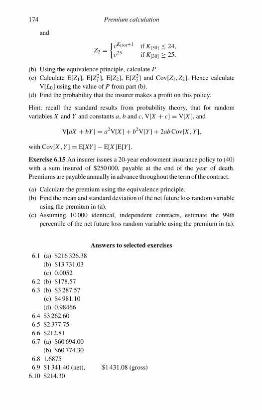
174 Premium calculation
and
Z2 ={vK[30]+1 if K[30] ≤ 24,v25 if K[30] ≥ 25.
(b) Using the equivalence principle, calculate P.(c) Calculate E[Z1], E[Z2
1 ], E[Z2], E[Z22 ] and Cov[Z1, Z2]. Hence calculate
V[L0] using the value of P from part (b).(d) Find the probability that the insurer makes a profit on this policy.
Hint: recall the standard results from probability theory, that for randomvariables X and Y and constants a, b and c, V[X + c] = V[X ], and
V[aX + bY ] = a2V[X ] + b2V[Y ] + 2ab Cov[X , Y ],with Cov[X , Y ] = E[XY ] − E[X ]E[Y ].Exercise 6.15 An insurer issues a 20-year endowment insurance policy to (40)with a sum insured of $250 000, payable at the end of the year of death.Premiums are payable annually in advance throughout the term of the contract.
(a) Calculate the premium using the equivalence principle.(b) Find the mean and standard deviation of the net future loss random variable
using the premium in (a).(c) Assuming 10 000 identical, independent contracts, estimate the 99th
percentile of the net future loss random variable using the premium in (a).
Answers to selected exercises
6.1 (a) $216 326.38(b) $13 731.03(c) 0.0052
6.2 (b) $178.576.3 (b) $3 287.57
(c) $4 981.10(d) 0.98466
6.4 $3 262.606.5 $2 377.756.6 $212.816.7 (a) $60 694.00
(b) $60 774.306.8 1.68756.9 $1 341.40 (net), $1 431.08 (gross)
6.10 $214.30
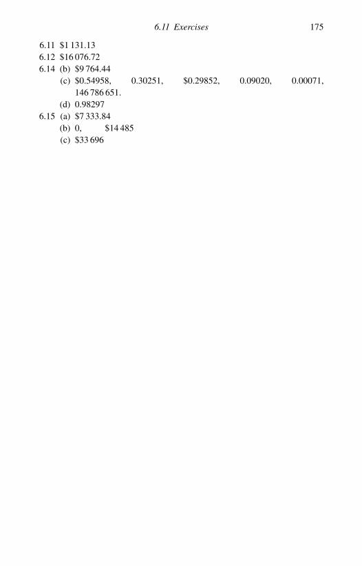
6.11 Exercises 175
6.11 $1 131.136.12 $16 076.726.14 (b) $9 764.44
(c) $0.54958, 0.30251, $0.29852, 0.09020, 0.00071,146 786 651.
(d) 0.982976.15 (a) $7 333.84
(b) 0, $14 485(c) $33 696