actors, actions, and uncertainties: optimizing decision-making … · 2019-11-18 · allows us to...

Solid Earth, 10, 2015–2043, 2019https://doi.org/10.5194/se-10-2015-2019© Author(s) 2019. This work is distributed underthe Creative Commons Attribution 4.0 License.

Actors, actions, and uncertainties: optimizing decision-makingbased on 3-D structural geological modelsFabian Antonio Stamm1, Miguel de la Varga1,2, and Florian Wellmann1

1Computational Geoscience and Reservoir Engineering (CGRE), RWTH Aachen University, Germany2Aachen Institute for Advanced Study in Computational Engineering Science (AICES), RWTH Aachen University, Germany

Correspondence: Fabian Antonio Stamm ([email protected])

Received: 15 March 2019 – Discussion started: 27 March 2019Revised: 11 September 2019 – Accepted: 16 September 2019 – Published: 18 November 2019

Abstract. Uncertainties are common in geological modelsand have a considerable impact on model interpretationsand subsequent decision-making. This is of particular signif-icance for high-risk, high-reward sectors. Recent advancesallows us to view geological modeling as a statistical prob-lem that we can address with probabilistic methods. Usingstochastic simulations and Bayesian inference, uncertaintiescan be quantified and reduced by incorporating additional ge-ological information. In this work, we propose custom lossfunctions as a decision-making tool that builds upon suchprobabilistic approaches.

As an example, we devise a case in which the decisionproblem is one of estimating the uncertain economic valueof a potential fluid reservoir. For subsequent true value esti-mation, we design a case-specific loss function to reflect notonly the decision-making environment, but also the prefer-ences of differently risk-inclined decision makers. Based onthis function, optimizing for expected loss returns an actor’sbest estimate to base decision-making on, given a probabilitydistribution for the uncertain parameter of interest. We applythe customized loss function in the context of a case studyfeaturing a synthetic 3-D structural geological model. A setof probability distributions for the maximum trap volume asthe parameter of interest is generated via stochastic simula-tions. These represent different information scenarios to testthe loss function approach for decision-making.

Our results show that the optimizing estimators shift ac-cording to the characteristics of the underlying distribution.While overall variation leads to separation, risk-averse andrisk-friendly decisions converge in the decision space and de-crease in expected loss given narrower distributions. We thusconsider the degree of decision convergence to be a mea-

sure for the state of knowledge and its inherent uncertaintyat the moment of decision-making. This decisive uncertaintydoes not change in alignment with model uncertainty but de-pends on alterations of critical parameters and respective in-terdependencies, in particular relating to seal reliability. Ad-ditionally, actors are affected differently by adding new in-formation to the model, depending on their risk affinity. It istherefore important to identify the model parameters that aremost influential for the final decision in order to optimize thedecision-making process.

1 Introduction

In studies of the subsurface, data availability is often limitedand characterized by high possibilities of error due to signalnoise or inaccuracies. This, together with the inherent epis-temic uncertainty of the modes, leads to the inevitable pres-ence of significant uncertainty in geological models, which inturn may affect interpretations and conclusions drawn from amodel (Wellmann et al., 2018, 2010a; de la Varga and Well-mann, 2016; de la Varga et al., 2019; Bardossy and Fodor,2004; Randle et al., 2019; Lark et al., 2013; Caers, 2011;Chatfield, 1995). Uncertainties are thus of particular impor-tance for making responsible and good decisions in relatedeconomic settings, such as in hydrocarbon exploration andproduction (Thore et al., 2002; McLane et al., 2008; Smal-ley et al., 2008). The quantification and visualization of suchuncertainties and their consequences is currently an activefield of research. Recent developments allow us to view geo-logical modeling as a statistical problem (see Wellmann andCaumon, 2018). We particularly regard approaches to couple

Published by Copernicus Publications on behalf of the European Geosciences Union.

2016 F. A. Stamm et al.: Actors, actions, and uncertainties

implicit geological modeling with probabilistic methods, aspresented by de la Varga et al. (2019) with the Python libraryGemPy.

Building on this probabilistic perspective, we propose theuse of custom loss functions as a decision-making tool whendealing with uncertain geological models. In many applica-tions, we are interested in some decisive model output value,for example reservoir volume. Given that such a parameteris the result of a deterministic function of uncertain variablesin our model, the parameter of interest is likewise uncertainand can be represented by a probability distribution attainedfrom stochastic simulations. A loss function can be appliedto such a distribution to return a case-specific best estimateto base decision-making on.

We consider hydrocarbon exploration and production asan exemplary high-risk, high-reward sector, in which gooddecision-making is crucial. However, the described meth-ods are potentially equally applicable to other types of fluidreservoirs (e.g., groundwater, geothermal, or CO2 seques-tration) and in the raw materials sector. Monte Carlo simu-lation for reservoir estimation and risk assessment has be-come common in this sector and is often used in combina-tion with decision trees (see Murtha, 1997; Mudford, 2000;Wim and Swinkels, 2001; Bratvold and Begg, 2010). How-ever, it seems to us that distributions resulting from proba-bilistic modeling are mostly only considered to attain bestestimates in the form of means. The most likely and ex-treme outcomes are identified as percentiles, typically P50(the median), P10, and P90. We believe that this practice doesnot harness the full potential of such a probabilistic distribu-tion and that much of the inherent information is discarded.Contrary to that, customized loss functions, as a Bayesianmethod, take into account the full probability distribution andenable the inclusion of various conditions in the process offinding an optimal estimate. While used in statistical deci-sion theory and other scientific fields, loss functions have, tothe best of our knowledge, found no significant applicationin the context of structural geological modeling. Thus, weintend to provide a new perspective with our methodology.

To illustrate our approach of using custom loss functionsfor decision-making, we first illustrate what such customiza-tion might look like step by step: starting off with a standardsymmetrical loss function, incorporating scenario-specificconditions and assumptions, and lastly implementing a fac-tor to represent the varying risk affinities of different de-cision makers. As we assume a petroleum exploration andproduction decision-making scenario, our parameter of in-terest should be one that indicates the economic value of apotential hydrocarbon accumulation. In a larger context, in-cluding various geological and economic factors such as op-erational expenditures, this could be the net present value(NPV) of a project. In preproduction stages, original oil inplace (OOIP) is commonly used for early assessments (Dean,2007; Morton-Thompson and Woods, 1993). Decision mak-ers would want to best estimate the relevant parameter of

interest to derive recoverable reserves, respective economicvalue, and subsequently allocate development resources ac-cordingly, which includes the possibility of walking awayfrom a prospect. In this case, the decision maker might referto an individual geological expert, but also to an explorationcompany as a whole.

Once we have set up a loss function customized to this de-cision problem, we can apply it to probability density func-tions that represent our knowledge about the true value ofthe parameter of interest. As mentioned above, such distribu-tions can result from geological modeling in a probabilisticcontext. To illustrate this, we include a synthetic 3-D struc-tural geological model as a case study. In this context, wedefine the structurally determined maximum trap volume Vtas our parameter of interest and indicator for economic value.We generate different probability distributions via stochasticsimulations and based on various information scenarios. It isimportant to note that these are always based on the sameprimary input parameters. We attain altered states of infor-mation by updating the reference case (prior) with secondaryinformation. In doing so, we make sure that the resulting dis-tributions and the realizations of loss function applicationscan be directly compared. These case studies are syntheticand chosen here to exemplify the application of Bayesian de-cision theory and to show how additional information affectsthe optimality of decisions.

2 Methods

2.1 Bayesian decision theory

We view the statistical analysis of geological models from aprobabilistic perspective, which is most importantly charac-terized by its preservation of uncertainty. Its principles havebeen presented and discussed extensively in the literature(see Jaynes, 2003; Box and Tiao, 2011; Harney, 2013; Gel-man et al., 2014; Davidson-Pilon, 2015). The Bayesian ap-proach is widely seen as intuitive and inherent in the naturalhuman perspective. It regards probability as a measure of be-lief about a true state of nature.

In many cases, decisions are made on the basis of sum-mary parameters such as mean or standard deviation. Thisapproximation works for well-defined probability distribu-tions but it may fail when the distribution does not have adefined structure, which is the usual case of distribution gen-erated as a result of Bayesian inference. In this work, weaim to tackle decision problems associated with probabilisticinferences. By applying Bayesian decision theory concepts,we are capable of transforming an arbitrary complex set ofdistributions onto a more adequate dimension for decision-making.

Solid Earth, 10, 2015–2043, 2019 www.solid-earth.net/10/2015/2019/

F. A. Stamm et al.: Actors, actions, and uncertainties 2017

2.1.1 Loss, expected loss, and loss functions

Common point estimates, such as the mean and the median ofa distribution, usually come with a measure for their accuracy(Berger, 2013). However, it has been argued by Davidson-Pilon (2015) that using pure accuracy metrics, while thistechnique is objective, ignores the original intention of con-ducting the statistical inference in cases in which payoffs ofdecisions are valued more than their accuracies. A more ap-propriate approach can be seen in the use of loss functions(Davidson-Pilon, 2015).

Loss is a statistical measure of how “bad” an estimate ofthe parameter /theta is. Estimate-based decisions are alsoreferred to as actions a. Therefore, we also refer to decisionmakers as actors. Loss is defined as L(θ,a), so L(θ1,a1) isthe actual loss incurred when action a1 is taken, while thetrue state of nature is θ1 (Berger, 2013). The magnitude ofincurred loss related to an estimate is defined by a loss func-tion, which is a function of the estimate and the true value ofthe parameter (Wald, 1950; Davidson-Pilon, 2015):

L(θ, θ̂)= f (θ, θ̂). (1)

So, how “bad” a current estimate is depends on the way aloss function weights accuracy errors and returns respectivelosses. Two standard loss functions are the absolute-error andthe squared-error loss function. Both are objective, symmet-ric, simple to understand, and commonly used.

The presence of uncertainty during decision-making im-plies that the true parameter value is unknown and thus thetruly incurred loss L(θ,a) cannot be known at the time ofmaking the decision. The Bayesian perspective considers un-known parameters to be random variables and samples thatare drawn from a probability distribution to be possible re-alizations of the unknown parameter; i.e., all possible truevalues are represented by this distribution.

Under uncertainty, the expected loss of choosing an es-timate θ̂ over the true parameter value θ is defined by(Davidson-Pilon, 2015)

l(θ̂ )= Eθ [L(θ, θ̂)]. (2)

The expectation symbol E is subscripted with θ , by whichit is indicated that θ is the respective unknown variable. Thisexpected loss l is also referred to as the Bayes risk of estimateθ̂ (Berger, 2013; Davidson-Pilon, 2015).

By the law of large numbers, the expected loss of θ̂ canbe approximated by drawing a large sample size N from theposterior distribution, applying a loss function L, and aver-aging over the number of samples (Davidson-Pilon, 2015):

1N

N∑i=1

L(θi, θ̂ )≈ Eθ [L(θ, θ̂)] = l(θ̂ ). (3)

Hereby, we can approximate the expected loss l for everypossible estimate θ̂ (every decision we can make) according

to the loss function in use. Minimization of a loss function re-turns a point estimate known as a Bayes action or a Bayesianestimator, which is the decision with the least expected lossaccording to the loss function and the decision in which weare interested in this work (Berger, 2013; Moyé, 2006).

2.1.2 Customization of our case-specific loss function

Davidson-Pilon (2015) and Hennig and Kutlukaya (2007)have proposed that it might be useful to move on from stan-dard objective loss functions to the design of customizedloss functions that specifically reflect an individual’s (i.e.,the decision maker’s) objectives and preferences regardingoutcomes. Especially as we assign an economic notion to ge-ological models and related estimation problems, we arguethat it is necessary to consider the subjective perspectivesof involved decision makers, for example exploration andproduction companies. Consequently, the design of a morespecific nonstandard and possibly asymmetric loss functionmight be required, one that includes subjective aspects anddifferences in weighting of particular risks, arising from adecision maker’s inherent preferences and the environmentin which this actor has to make a decision. In the face ofseveral uncertain parameters, which is a given in complexgeological models, a perfect estimate, a perfect decision, isvirtually unattainable. However, an attempt can be made todesign a custom loss function that returns a Bayesian estima-tor involving the least bad consequences for a decision makerin a specific environment (Davidson-Pilon, 2015; Hennig andKutlukaya, 2007).

Hennig and Kutlukaya (2007) argue that choosing and de-signing a loss function involves the translation of informalaims and interests into mathematical terms. This process nat-urally implies the integration of subjective elements. Accord-ing to them, this is not necessarily unfavorable or less objec-tive, as it may better reflect an expert’s perspective on thesituation.

Standard symmetric loss functions can easily be adapted tobe asymmetric, for example by weighting errors to the neg-ative side stronger than those to the positive side. Preferenceover estimates larger than the true value, i.e., overestimation,is thus incorporated in an uncomplicated way. Much morecomplicated designs of loss functions are possible, depend-ing on purpose, objective, and application. We will describepotential design options in the following.

For our example of estimating the economic value of a hy-drocarbon prospect, which is represented by the maximumtrap volume Vt, we develop a custom loss function in fivesteps. Ideally, a decision maker would like to know the exacttrue value so that resources can be allocated appropriately inorder to acquire economic gains by developing a project andproducing from a reservoir. This conscious and irrevocableallocation of resources is the decision to be made or action tobe taken (Bratvold and Begg, 2010). Thus, we treat estimat-ing as equivalent to making a decision. Deviations from the

www.solid-earth.net/10/2015/2019/ Solid Earth, 10, 2015–2043, 2019


unknown true value in the form of over- and underestimationbring about an error and loss accordingly.

It can be assumed that several decision makers in one suchenvironment or sector may have the same general loss func-tion but different affinities concerning risks. This might bebased, for example, on different psychological factors or eco-nomic philosophies followed by companies. It might also bebased on the budgets and options such actors have available.An intuitive example is the comparison of a small and a largecompany. A false estimate and wrong decision might have asignificantly stronger impact on a company that has a gen-erally lower market share and few projects than on a largercompany that might possess higher financial flexibility andfor which one project is only one of many development op-tions in a wide portfolio.

In steps I–IV we make assumptions about the significanceof such deviations and how they differently contribute to ex-pected losses in the general decision-making environmentand introduce the concept of varying risk affinities in the finalstep V.

– Step I – Choosing a standard loss function as a startingpoint. In our case, we assume that investments increaselinearly with linear growth in the value of the prospect.For this reason, we choose the symmetric absolute-errorloss function as a basis for further customization steps:

L(θ, θ̂)= |θ − θ̂ |. (4)

– Step II – Simple overestimation. Considering the devel-opment of a hydrocarbon reservoir, it can be assumedthat over-investing is worse than under-investing. Over-estimating the size of an accumulation might, for ex-ample, lead to the installation of equipment or facilitiesthat are actually redundant or unnecessary. This wouldcome with additional unrecoverable expenditures. Con-sequences from underestimating (0< θ̂ < θ ), however,may presumably be easier to resolve. Additional equip-ment can often be installed later on. Hence, simple over-estimation (0< θ < θ̂ ) is weighted stronger in this lossfunction by multiplying the error with an overestimationfactor a:

L(θ, θ̂)= |(θ − θ̂ )| a. (5)

– Step III – Critical overestimation. The worst case forany project would be that its development is set intomotion expecting a gain only to discover later that thevalue in the reservoir does not cover the costs of realiz-ing the project, resulting in an overall loss. A petroleumsystem might also turn out to be a complete failure con-taining no value (Vt = 0 in our 3-D case study) at all, al-though the actor’s estimate indicated the opposite. Here,we refer to this as critical overestimation. A positivevalue is estimated, but the true value is zero or negative

(θ ≤ 0< θ̂ ). This is worse than simple overestimation,whereby both values are positive and a net gain is stillachieved, which is only smaller then the best possiblegain of expecting the true value. Critical overestimationis included in the loss function by using another weight-ing factor b that replaces a:

L(θ, θ̂)= |(θ − θ̂ )| b. (6)

In other words, with b = 2, critical overestimation istwice as bad as simple overestimation.

– Step IV – Critical underestimation. We also derive criti-cal underestimation from the idea of estimating zero (ora negative value) when the true value is actually positive(θ̂ ≤ 0< θ ). This is assumed to be worse than simpleoverestimation but clearly better than critical overesti-mation. No already owned resources are wasted, andit is only the potential value that is lost, i.e., opportu-nity costs that arise from completely discarding a prof-itable project. Critical underestimation is weighted us-ing a third factor c:

L(θ, θ̂)= |(θ − θ̂ )| c. (7)

– Step V – Including different risk affinities. We now fur-ther adapt the loss function to consider varying riskaffinities of different actors. We follow the approach ofDavidson-Pilon (2015), who implemented different riskaffinities by simply introducing a variable risk factor.Using different values for this factor, we can representhow comfortable an individual is with being wrong andfurthermore which “side of wrong” is preferred by thatdecision maker (Davidson-Pilon, 2015). In our case,bidding lower is considered the cautious, risk-averse op-tion, as smaller losses can be expected from underes-timating. Guessing higher is deemed riskier, as lossesfrom overestimation are greater. However, bidding cor-rectly on a higher value will also return a greater gain. Itis assumed that risk-friendly actors care less about crit-ical underestimation; i.e., they would rather develop aproject than discard it. In our finalized loss function, wesimply include these considerations via a risk affinityfactor r , which alters the incurred losses:

L(θ, θ̂)=

|θ − θ̂ | r−0.5, for 0< θ̂ < θ|θ − θ̂ | a r, for 0< θ < θ̂|θ − θ̂ | b r, for θ ≤ 0< θ̂|θ − θ̂ | c r−0.5, for θ̂ ≤ 0< θ

,

with a,b,c,r ∈Q. (8)

This equation shows that the final custom loss function is inessence a composite of four different functions for the over-and underestimation cases explained in steps II–IV. It is im-portant to note that the weighting factors a, b, and c can take



basically any numerical values but should be chosen in a waythat they appropriately represent the framework conditions ofthe problem. Here, we assume that simple overestimation is25 % (a = 1.25), critical overestimation 100 % (b = 2), andcritical underestimation 50 % (c = 1.5) worse than simpleunderestimation.

According to Eq. (8), the risk-neutral loss function is re-turned for r = 1, as no reweighting takes place. For r < 1,the weight on overestimating (a, b) is reduced and increasedfor critical underestimation (c), as well as normal underesti-mation. This represents a risk-friendlier actor that is willingto bid on a higher estimate to attain a greater gain. For r > 1,the overestimation weight (a, b) is increased in the loss func-tion, underestimation and critical underestimation weight (c)are decreased, and more risk-averse actors are prompted tobid on lower estimates. Since risk neutrality is expressed byr = 1, we consider values 0< r < 2 to be the most appropri-ate choices to represent both sides of risk affinity equally.

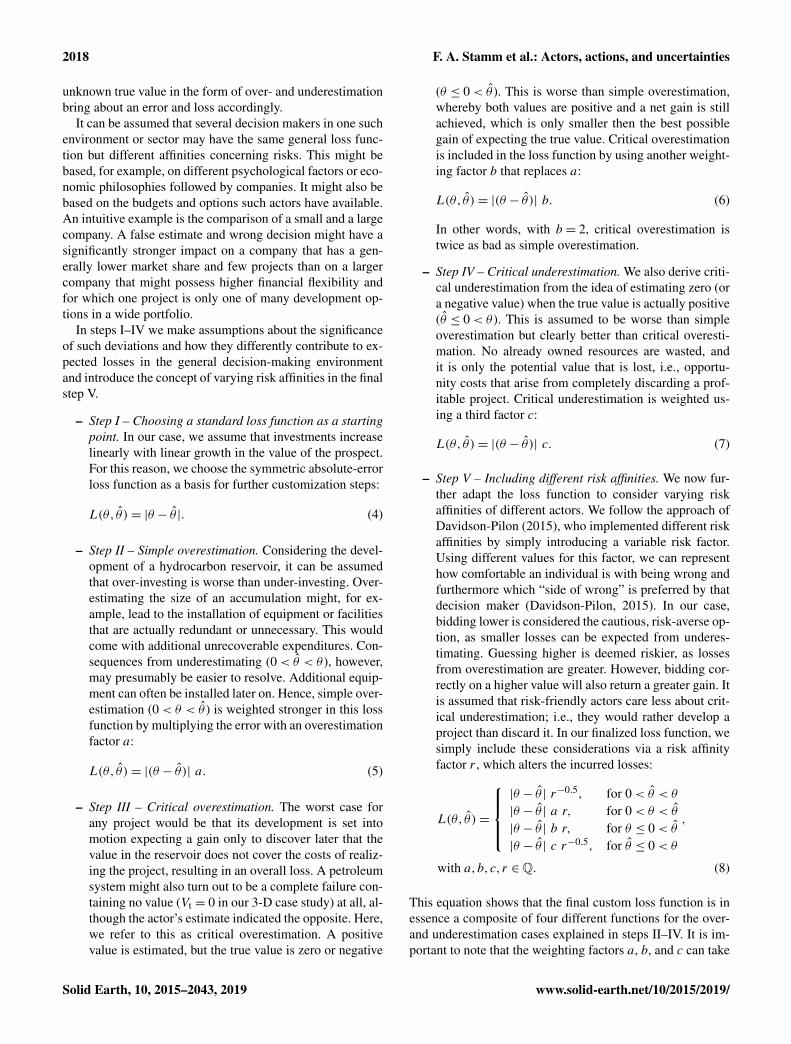
In Fig. 1, we illustrate different aspects and steps of adapt-ing and applying the custom loss function. For these simpleexamples, we assume that the economic value of our reser-voir is represented by an abstract score parameter. Figure 1adepicts the plotting of the absolute-error loss function (cus-tomization step I) applied to a normal distribution. It can beseen that for this standard symmetrical function, the mini-mal point of expected losses and Bayes action correspondsto the median (and mean for this symmetric distribution).Figure 1b summarizes customization steps II–IV and visual-izes how four different functions for four cases of under- andoverestimation are summed up to one combined loss functionthat comprises all of the assumptions made for the decision-making environment. A jump of expected losses on the nega-tive side of possible estimates can be attributed to the way wedefined the function for critical underestimation as dependenton zero.

In Fig. 1c, the risk factor of step V was implemented with-out steps II–IV, i.e., only for the standard absolute-error lossfunction. It can be seen that risk-averse and risk-friendly de-cision makers are represented by different realizations of ex-pected losses based on one and the same normal distribution:the narrow shape of the risk-friendly function represents im-proved confidence in the decision, while the increased ex-pected loss (Bayes risk) of the minimum indicates that thiscomes along with the acceptance of a higher risk. Inversely,the flat shape of the risk-averse function can be seen as re-duced confidence in the decision. There is less of a differencein making a different decision than for the risk-friendly ac-tor. At the same time, the expected loss of the minimum, andthus the accepted risk, is lower. However, although they differin expected losses, both decision makers share the same in-dividual best estimate, since the loss function in itself is stillsymmetric. This changes in panel (d), in which all customiza-tion steps were applied. Here, the risk factor reweights theinfluence of the subfunctions shown in panel (b). Under- andoverestimation cases are accordingly enhanced or reduced in

impact so that the resulting loss function becomes asymmet-ric and minima are found at different score estimates, giventhe same underlying information.

In Fig. 1e and f, the functions from panels (c) and (d) areapplied on a score distribution resulting from the combina-tion of two other uncertain parameters: reservoir thicknessand depth. This can be seen as an extremely simplified 1-Dmodel with only two inputs that define one output as a param-eter of interest, the final score. In this case, thickness is seenas the potential positive value in our reservoir, as it providesspace for hydrocarbons to accumulate. Depth is subtractedfrom this, as it implies a cost of drilling. Thus, the final scoreis a very essential representation of the economic value giventhe information available. The respective final distribution isslightly skewed. Figure 1e depicts the respective applicationof the same functions used in panel (c): symmetric, but in-cluding risk affinity. The overall effects are the same as inpanel (c). It can be additionally observed that since the under-lying distribution is now asymmetric, all expected loss min-ima are found on the median estimate, lower than the mean.In panel (f), the complete custom loss function was appliedas in panel (d). Based on the uncertain information about thefinal score, the three differently risk-affine loss functions plotdifferently, with minima in the negative space, at zero, and inthe positive space. This illustrates how the risk-averse de-cision maker tends to expect a possible negative outcome,while the risk-friendly actor bids on a positive value. Thiscould be seen as the decision to abandon versus the decisionto invest in a prospect.

For a better understanding of how our finalized customloss function determines the incurrence of loss, actual lossesfor three fixed true values and risk neutrality (r = 1) are plot-ted in Fig. 2.

It has to be emphasized that this is just one possible pro-posal for loss function customization. There is not one per-fect design for such a case (Hennig and Kutlukaya, 2007).Slight to strong changes can already be implemented by sim-ply varying the values of the weighting factors a, b, and c.Fundamentally different loss functions can also be based ona significantly different mathematical structure. As loss func-tions are customized regarding the problem environment andaccording to the subjective needs and objectives of the de-cision maker, they are mostly defined by the actor express-ing his or her perspective (Davidson-Pilon, 2015; Hennig andKutlukaya, 2007). Changes in the individual’s perception andattitude might lead to further customization needs at a futurepoint in time, as reported by Hennig and Kutlukaya (2007).

2.2 Case study: synthetic 3-D structural geologicalmodel

Next we want to show that this loss function approach is notonly applicable to simple probability distributions but is anequally useful tool to estimate the true value of a parameter ofinterest resulting from more complex geological models that



Figure 1. Illustration of different steps and aspects of our loss function customization. Functions are applied to an abstract score as theparameter of interest.

encompass numerous uncertain input parameters. As a casestudy, we now consider a synthetic 3-D structural geologicalmodel that is placed in a probabilistic framework.

2.2.1 Computational implementation

Computationally, we implement all of our methods in aPython programming environment, relying in particular onthe combination of two open-source libraries: (1) GemPy(version 1.0) for implicit geological modeling and (2) PyMC(version 2.3.6) for conducting probabilistic simulations.

GemPy is able to generate and visualize complex 3-Dstructural geological models based on a potential-field in-terpolation method originally introduced by Lajaunie et al.

(1997) and further elaborated by Calcagno et al. (2008).GemPy was specifically developed to enable the embeddingof geological modeling in probabilistic machine-learningframeworks, in particular by coupling it with PyMC (de laVarga et al., 2019).

PyMC was devised for conducting Bayesian inferenceand prediction problems in an open-source probabilisticprogramming environment (Davidson-Pilon, 2015; Salvatieret al., 2016). Different model-fitting techniques are providedin this library, such as various Markov chain Monte Carlo(MCMC) sampling methods. For our purpose we make useof adaptive metropolis sampling by Haario et al. (2001) andcheck MCMC convergence via a time series method ap-



Figure 2. Loss based on the risk-neutral custom loss function(Eq. 8) for determined true scores of −250, 0, and 250. This plotis meant to clarify the way real losses are incurred for each esti-mate relative to a given true value. The expected loss, as seen inFig. 1, is acquired by arithmetically averaging over all deterministicloss realizations based on the score probability distribution by usingEq. (3).

proach by Geweke (1991). Components of a statistical modelare represented by deterministic functions and stochasticvariables in PyMC (Salvatier et al., 2016). We can thus usethe latter to represent uncertain model input parameters andlink them to additional data via likelihood functions. Otherparameters, such as the value of interest for decision-making,can be determined over deterministic functions as children ofparent input parameters.

To visually compare the states of geological unit probabil-ities after conducting stochastic simulations, we consider thenormalized frequency of lithologies in every single voxel andvisualize the results in probability fields (see Wellmann andRegenauer-Lieb, 2012).

2.2.2 Design of the 3-D structural geological model

Our geological example model is designed to represent apotential hydrocarbon trap system. Stratigraphically, it in-cludes one main reservoir unit (sandstone), one main sealunit (shale), an underlying basement, and two overlying for-mations that are assumed to be permeable so that hydrocar-bons could have migrated upwards. Structurally, it is con-structed to feature an anticlinal fold that is displaced by anormal fault. All layers are tilted and dip in the opposite di-rection of the fault plane dip. A potential hydrocarbon trapis thus found in the reservoir rock enclosed by the deformedseal and the normal fault.

Using GemPy, we construct the geological model as fol-lows: in principle, it is defined as a cubic block with an extentof 2000 m in the x, y, and z directions. The basic input datafor the interpolation of the geological features is composed of

Table 1. Input parameter uncertainties defined by distributions withrespective means µ, standard deviations σ , and shape factor α.

µ σ α

Overlying 0 40 0Sandstone 2 0 60 0Seal 0 80 0Reservoir 0 100 0Fault offset 0 −150 −2

3-D point coordinates for layer interfaces and fault surfaces,as well as orientation measurements that indicate respectivedip directions and angles. From these data, GemPy is able tointerpolate surfaces and compute a voxel-based 3-D model(see Fig. 3).

We include uncertainties by assigning them to the z po-sitions of points that mark layer interfaces in the 3-D space.This is achieved via probability distributions (PyMC stochas-tic variables) from which error values are drawn. These arethen added to the original input data z value. As the z positionis the most sensible parameter for predominantly horizontallayers, we can hereby not only implement uncertainties re-garding layer surface positions in depth, but also layer thick-nesses, geometrical shapes, and degree of fault offset.

Such probability distributions can also be allocated ashomogeneous sets to point and feature groups that are toshare a common degree of uncertainty (see Table 1). We as-sign the same base uncertainty to groups of points belong-ing to the same layer bottom surface by referring them toone shared distribution each. Assuming an increase in un-certainty with depth, standard deviations for the shared dis-tributions are increased for deeper formations. Furthermore,uncertainty regarding the magnitude of fault offset is incor-porated by adding a skewed normal probability distributionthat is shared by all layer interface points in the hanging wall.A left-skewed normal distribution is chosen to reflect the na-ture of throw on a normal fault, in particular the slip motionof the hanging wall block. Skew to the negative side ensuresthat the offset nature of the normal fault is maintained andinversion to a reverse fault is avoided.

This model was designed for the primary purpose of test-ing our loss function method. All features, uncertainties, andparameter relations were implemented in a way that they re-sult in model variability and complexity that is adequate andsignificant to the decision problem in this work. The model isnot aimed at representing a completely plausible or realisticgeological setting.

2.2.3 Vt as the parameter of interest

Given full 3-D representation of geological structures, wecan now define the trap volume Vt as the parameter of inter-est, a feature that indicates the economic value of the reser-voir in this case. For conducting straightforward volumetric



Figure 3. Design of the 3-D structural geological model. A 2-D cross section through the middle of the model (y = 500 m), perpendicularto the normal fault (parallel to the x–z plane), is shown in (a). A 3-D voxel representation of the model, highlighting the reservoir and sealformations, is visualized in (b). In (c) and (d), the inclusion of parameter uncertainties is presented. Colors indicate certain layer bottoms(i.e., boundaries) that are assigned shared z-positional uncertainties (c). All points in the hanging wall are additionally assigned a fault offsetuncertainty (d). Thicknesses of the three middle layers are defined by the distances of boundary points (e) and are thus directly dependenton (c).

calculations, we assume that closed traps are always filledto spill; i.e., we only consider structural features as control-ling mechanisms and disregard other parameters in the OOIPequation (Eq. 9).

We argue that Vt can be inserted for the hydrocarbon-filledrock volumeA·h in the OOIP equation (Dean, 2007; Morton-Thompson and Woods, 1993):

OOIP= A ·h ·φ · (1− SW) · 1/FvF, (9)

where OOIP is returned in cubic meters, A is the drainagearea, h the net pay thickness, φ the porosity, SW the watersaturation, and FvF the formation volume factor that deter-mines the shrinkage of the oil volume brought to the surface.

By declaring these connections, we have given our modelan economic significance. We can assume that the hydrocar-bon trap volume is directly linked to project development de-cisions; i.e., the investment and allocation of resources is rep-resented by bidding on a volume estimate.

In the course of this work, we developed a set of algo-rithms to enable the automatic recognition and calculation

of trap volumes in geological models computed by GemPy.The volume is determined on a voxel-counting basis via fourconditions illustrated in Fig. 4 and further explained in Ap-pendix A.

Following these conditions, we can define four majormechanisms that control the maximum trap volume: (1) theanticlinal spill point of the seal cap, (2) the cross-fault leakpoint at a juxtaposition of the reservoir formation with itself,(3) leakage due to juxtaposition with overlying layers andcross-fault seal breach (failure related to the shale smear fac-tor, SSF), and (4) stratigraphical breach of the seal when itsvoxels are not continuously connected above the trap. Due tothe nature of our model, (3) and (4) will always result in com-plete trap failure. The occurrence of these trap control mech-anisms can be tracked throughout stochastic simulations ofthe model.



Figure 4. Illustration of the process of trap recognition in 2-D, i.e., the conditions that have to be met by a model voxel to be accepted asbelonging to a valid trap. A voxel has to be labeled as part of the target reservoir formation (a) and positioned in the footwall (b). Trap closureis defined by the seal shape and the normal fault (c). Consequently, the maximum trap fill is defined by either the anticlinal spill point (S)or a point of leakage across the fault, depending on juxtapositions with layers underlying (L1) or overlying the seal (L2). The latter is onlyrelevant if the critical shale smear factor is exceeded, as determined over D and T in (d). In this example, assuming sealing of the fault dueto clay smearing, the fill horizon is determined by the spill point in (d). Subsequently, only trap section 1 is isolated from the model bordersin (d) and can thus be considered a closed trap. Voxels included in this section are counted to calculate the maximum trap volume.

2.2.4 Generating different probability distributions forVt

The trap volume Vt is a result from GemPy’s implicit geo-logical model computation. It is an output parameter depen-dent on deterministic and stochastic input parameters. Whenconducting stochastic simulations, input uncertainties willpropagate to Vt, which is thereby represented by a respec-tive probability distribution that our custom loss function canbe applied to. Using simple Monte Carlo error propagation,with every iteration, we draw sample values for our uncer-tain primary model input parameters defined in Sect. 2.2.2,and thus, with every iteration, we create one possible realiza-tion of our geological model, which in turn comes with onepossible outcome for Vt. Results from all iterations togetherapproximate the probability distribution for Vt according tothe input parameters.

Furthermore, we consider the possibility of updatingour model by adding additional secondary information viaBayesian inference. We do this by introducing likelihoodfunctions that constrain our primary parameters. We have tonote that these inputs remain unchanged; however, their priorprobability distributions are revalued given the additional sta-tistical information. We achieve this by conducting Markovchain Monte Carlo (MCMC) simulations. Decision-makingis then based on the resulting posterior probability. Using dif-ferent likelihood functions, we can create and generate differ-ent posterior probability distributions for Vt, which representdifferent information scenarios. Since we use Bayesian infer-ence to revalue our original prior inputs, we can compare alloutcomes and realizations of our custom loss function.

For the application of Bayesian inference, we implementtwo types of likelihoods.



1. Layer thickness likelihoods. With every model realiza-tion, we extract the z distance between layer bound-ary input points at a central x–y position (x = 1100 m,y = 1000 m) in our input interpolation data. Resultingthicknesses can then be passed on to stochastic func-tions in which we define thickness likelihoods via nor-mal distributions.

2. Shale smear factor (SSF) likelihood. SSF values are re-alized over more complex parameter compositions. Webase this likelihood on a normal distribution that we linkto the geological model output.

The inclusion of these likelihoods is based on purely hypo-thetical assumptions and is intended to provide the opportu-nity to explore the effects that different types and scenarios ofadditional information might have. While the thickness like-lihood functions are dependent on input parameters directly,the implementation of the SSF likelihood function requiresa full computation of the model and extended algorithms ofstructural analysis.

Although Bayesian inference was utilized in this casestudy, it served primarily for the generation of these differentbut comparable distributions on which to base our decision-making, i.e., the application of our custom loss function. Foradditional information on how implicit geological modelingcan be embedded in a Bayesian framework and how this canbe used to reduce uncertainty, we refer to the work by Well-mann et al. (2010b), de la Varga and Wellmann (2016), de laVarga et al. (2019), and Wellmann et al. (2017).

3 Results

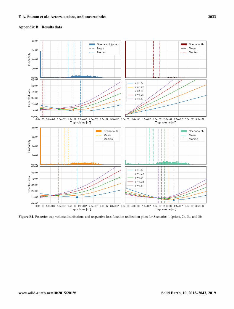
We applied our custom loss function to various differentVt probability distributions resulting from stochastic simu-lations. First, reference results were created using only pri-mary inputs (priors) and simple Monte Carlo error prop-agation (10 000 sampling iterations, Scenario 1). Then wedevised several scenarios of additional information and in-cluded these via likelihoods and Bayesian inference. For this,10 000 MCMC sampling steps were conducted, with an ad-ditional burn-in phase of 1000 iterations. The prior parame-ter uncertainties were chosen to be identical for all simula-tions (see Table 1). Results of convergence diagnostics canbe found in Appendix C.

We present the following information scenarios.

1. Prior-only model

2. Introducing seal thickness likelihoods

a. Likely thick seal

b. Likely thin seal

3. Introducing reservoir thickness likelihoods

a. Likely thick reservoir

b. Likely thick reservoir and thick seal

4. Introducing SSF likelihoods

a. SSF likely near its critical value

b. Likely reliable SSF and thick seal

The implemented likelihoods are listed in Table 2.For the comparison of results, we consider in particular

the following measures: (1) probability field visualization,(2) occurrence of trap control mechanisms, (3) resulting trapvolume distributions, and (4) consequent realization of ex-pected losses and related decisions.

3.1 Prior-only model (Scenario 1)

Probability field visualization illustrates well how the prioruncertainty is based on normal distributions (see Fig. B2).Trap control mechanisms are listed in Table B2. For thisprior-only scenario, all four relevant mechanisms occur. Thedominant factor is the anticlinal spill point with a 51.5 %rate of occurrence. It is followed by cross-fault leakage tothe reservoir (25 %) and other permeable formations (12 %).Stratigraphical breaches of the seal were registered to be de-cisive in about 11 % of iterations. In only 0.5 % of iterations,the algorithm failed to recognize a mechanism; i.e., correctmodel realization failed.

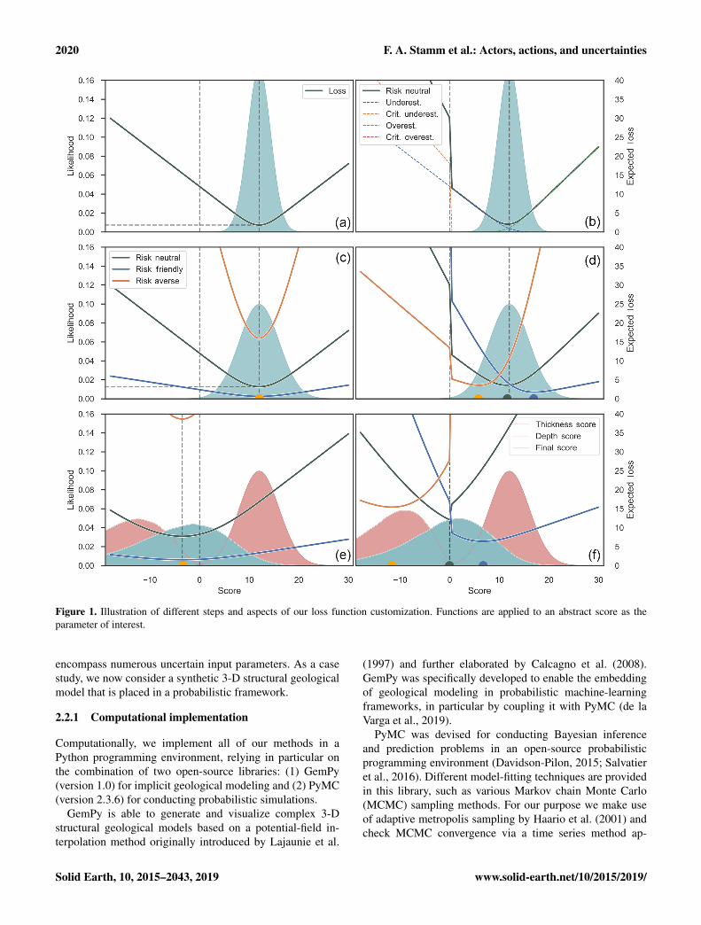
Maximum trap volumes were calculated for each modeliteration and plotted as a probability distribution in Fig. 5.In general, a wide range of volumes is possible, from zeroto more than 3 million m3. However, we can recognize a bi-modal tendency: low volumes are less probable than signifi-cantly high volumes or complete failure (Vt = 0).

Consequently, applying our custom loss function to thisdistribution resulted in widely separated minimizing estima-tors for the differently risk-inclined actors (see Fig. 5). Onlythe risk-friendliest estimates are found within the describedhighly positive mode of the distribution. Risk-averse individ-uals bid on significantly lower estimates or even zero. Therisk-neutral decision is found between the two modes andpresents the highest expected loss. Expected losses decreasetowards the extreme decisions and closer to the modes.

3.2 Introducing seal thickness likelihoods (Scenarios 2aand 2b)

We considered two scenarios of thickness likelihoods: theseal being (Scenario 2a) likely very thick or (Scenario 2b)likely very thin (see Table 2).

In Scenario 2a, probability visualization illustrates that thepresence of a thick seal is very probable (see Fig. B2). ForScenario 2b, the presence of a reliable seal is questionable.

A high likelihood of a reliable seal cap (2a) significantlyreduced the probability of trap failure, while enhancing themode of highly positive outcomes (see Fig. 5). This coincideswith the predominance of the anticlinal spill point (63 %) and



Table 2. Normal distribution mean (µ) and standard deviations (σ ) for the likelihoods implemented in the different scenarios.

Seal thickness Reservoir thickness SSF

µ (m) σ (m) µ (m) σ (m) µ σ

Scenario 1 – – - – – -Scenario 2a 300 30 - – – -Scenario 2b 50 30 - – – -Scenario 3a 350 30 - – – -Scenario 3b 300 30 300 30 – -Scenario 4a – – - – 5.1 0.3Scenario 4b 300 30 - – 2 0.3

Figure 5. Trap volume distribution and resulting loss function realizations for Scenario 1 (prior) and Scenario 2a, in which we introduced thelikelihood of a thick seal. Comparing both, we can observe how the additional information reduced the bimodality in the posterior distribution(2a), particularly by reducing the probability of complete failure and enhancing positive probabilities. Consequently, Bayes actions convergedand expected losses were reduced.

the leak point to the same reservoir (36 %) as control mech-anisms. The occurrence of other mechanisms was negligi-ble (see Table B2). Inversely, a likely thin seal (2b) virtuallyeliminated the positive mode and focused almost the wholedistribution on complete failure. Accordingly, seal-breach-related control mechanisms gained importance (65.5 % oc-currence rate for stratigraphical seal breach).

In both scenarios, Bayes actions shifted towards the re-spectively emphasized modes. This came with the overallconvergence of decisions and reduction of expected losses.In Scenario 2a, all decision makers bid on a positive out-come. Risk-averse individuals experienced the strongest shiftbut also present the highest expected losses. In Scenario 2b,all individuals decide not to allocate resources. Even the risk-friendliest actor moved to a zero estimate, with the most risk-averse bid having already been placed in the prior Scenario 1.

However, although all decisions coincide, expected losses in-crease from risk averse to risk friendly (see Table B1).

3.3 Introducing reservoir thickness likelihoods(Scenarios 3a and 3b)

We also tested scenarios for the likelihood of a thick reser-voir formation alone (Scenario 3a) and in combination withthe likelihood of a thick seal (Scenario 3b; see Table 2).The overall effect of using these reservoir-based likelihoodsturned out to be minor compared to the seal-related scenar-ios.

In Scenario 3a, failure probabilities slightly increased, re-sulting in a decision shift towards lower values (see Fig. B1).Results for Scenario 3b are very similar to those of 2b, ascan also be seen in Table B1. There was no significant re-duction of expected losses or a shift in decisions by adding



Figure 6. Probability field visualizations for seal and reservoir units in Scenarios 1 (prior), 4a, and 4b. For Scenario 1, we used 3-D voxelvisualizations and set a threshold at a probability of 0.5 (only voxels with a probability higher than 0.5 are shown). It can be recognized thatthe seal is disrupted across the fault in more than 50 % of the prior model realizations. For the other scenarios, we show the full probabilityfield for both units on a section through the middle of the model (y = 500 m), parallel to the x–z plane.

the likelihood of a thick reservoir to the likelihood of a thickseal.

3.4 Introducing SSF likelihoods

We considered two SSF-related likelihood scenarios. In Sce-nario 4a, we implemented solely an SSF likelihood that wasbased on a narrow normal distribution (µ= 5.1, σ = 0.3)with a mean near the critical value SSFc = 5. In Scenario 4b,we combined the likelihood of a thick seal (2a) with a likelymoderate but reliable SSF value (SSF normal distributionwith µ= 2 and σ = 0.3). Figure 6 illustrates the posteriorsituations well.

Scenario 4a resulted in increased bimodality of the pos-terior distribution (see Fig. 7). Accordingly, the Bayes ac-tion divergence and expected losses increased. Only two trapcontrol mechanisms remained relevant for 4a (see Table B2):anticlinal spill (66 %) and cross-fault leakage to overlyingformations (34 %).

The results for 4b were comparable to those of 2a butmore pronounced. Entropies, particularly related to the sealthickness, were clearly reduced, also in the hanging wall.Probabilities of failure and low volumes were almost elimi-nated, further enhancing the highly positive mode. This con-

sequently resulted in an even higher convergence of Bayesactions, as well as reduction of expected losses compared toScenario 2a. Anticlinal spill is the decisive control mecha-nism in 79.5 % of cases; otherwise, only cross-fault leakageto the reservoir occurred (20.5 %).

4 Discussion

Our results show that it is possible to apply Bayesian deci-sion theory to geological models as an approach to obtain anobjective basis for decisions by considering uncertainties inthese models. Even though the concept itself is not new, theapplication to the context of probabilistic geological mod-eling requires some adaptation and care when constructingappropriate loss functions. Our results highlight the potentialuse of custom loss functions, first for a simplified 1-D case,and then for a more complex full 3-D model. Even thoughthese models are both conceptual, they highlight in our pointof view the interesting potential of the method, as the opti-mal decision, the Bayes action, is not always directly obvi-ous when only considering posterior predictive distributions.The addition of subjective risk affinity and the risk of criticaloverestimation particularly lead to interesting changes in the



Figure 7. Trap volume distribution and resulting loss function realizations for Scenario 4a and Scenario 4b. Adding a likelihood of theSSF being around its critical value led to increased bimodality and an elimination of low to moderate volume probabilities. Bayes actionsdiverged accordingly in Scenario 4a. Implementing a reliable SSF value likelihood (µ= 2, σ = 0.3) in combination with the thick seallikelihood from Scenario 2a resulted in an emphasis on highly positive volumes. This, in turn, led to a stark convergence of decisions andreduction of expected losses.

optimal decision. Given these aspects, we consider the useof custom loss functions with probabilistic geological mod-eling to be a very suitable combination in the framework ofBayesian decision theory.

The case study considered here addressed a typical sce-nario of exploration for a fluid reservoir. We first discuss ad-ditional relevant points with regard to this specific case andthen provide more general comments on extensions and theapplication in additional fields in which geological modelsare commonly used.

4.1 State of knowledge, decision uncertainty, andconsistent decision-making

As we defined trap volume to be in essence a determinis-tic function of uncertain model input parameters, uncertain-ties propagate to this parameter of interest when conduct-ing stochastic simulations. We consider the resulting volumeprobability distributions to be expressions of the respectivestate of knowledge (or information) on which the decision-making is to be based. As this should include all parametersand conditions relevant for decision-making, we furthermorepropose that the overall uncertainty inherent in this probabil-ity distribution can be referred to as “decision uncertainty”and that this entity should be viewed separately from geolog-ical model uncertainty.

By viewing decision-making as a problem of optimizing acase-specific custom loss function applied to such a state ofknowledge and decision uncertainty, we were able to observe

clear differences in the respective behavior of distinctly risk-inclined actors.

The position and separation of their minimizing estima-tors, i.e., their decisions, manifested according to the proper-ties of the value distributions. The general spread and the oc-currence of modes relative to the overall distribution and therelevant decision space appear to be particularly significant.High spread and bimodal tendencies, i.e., high overall uncer-tainty, resulted in a wider separation of different actions. Re-duction of the distribution to one mode conversely led to theirconvergence. A decrease in decision uncertainty was further-more accompanied by a reduction in expected loss for eachBayes estimator.

Considering these observations, we derive the degree ofaction convergence and respective expected losses as mea-sures for the state of knowledge and decision uncertainty atthe moment of making a decision. The better these are, themore similar the decisions of differently risk-inclined actorsand the lower their loss expectations are. Given perfect in-formation all actors would bid on the same estimate (the truevalue) and expect no loss, since no risk would be present. Itfurthermore follows from this that the relevance of risk affin-ity decreases with greater reduction of decision uncertainty.

4.2 On the impact of additional information ondecision-making

We used these loss-function-related indicators to assess thesignificance of additional information for decision-making.



We observed that the impact on decision uncertainty, in-duced by Bayesian inference, is not simply strictly alignedwith the change in uncertainty regarding model parametersbut on parameter combinations that are relevant for the out-come of the value of interest. It seems to be of central im-portance (1) “where” in the model uncertainty is reduced,i.e., in which spatial area or regarding which model parame-ters, and (2) which possible outcome is enhanced in termsof probability. An increased probability of a thick or thinseal in our model equally reduced decision uncertainty sig-nificantly by raising the probability of a positive or negativeoutcome, respectively. Improved certainty about our reser-voir thickness, however, had far lesser impact on decision-making. This shows that some areas and parameter combi-nations have a much greater influence on the decision uncer-tainty than others, depending on the way they contribute tothe outcome of the value of interest.

Some types of additional information could even lead toincreased decision uncertainty. We observed this in Sce-nario 4a. The introduced SSF likelihood practically con-strained our geological model to two possible situations: (1) atrap that is sealed off from juxtaposing layers and full to spilland (2) complete failure of the trap due to a breached sealacross the fault. This made the decision problem a predomi-nantly binary one and split the outcome distribution into twonarrowed but distant modes. The resulting increase in deci-sion divergence and expected losses show that, in some cases,adding information might leave actors in greater disagree-ment than before.

However, we furthermore have to consider that actorsweight possible outcomes of the value distribution differ-ently. They are consequently affected differently by the sametype of information. Risk-friendly actors were the most ro-bust in their decision-making in the face of possible trapfailure. Eliminating this risk proved to be far less signifi-cant for the most risk-friendly than for risk-averse actors.Accordingly, it should be of foremost importance for risk-averse actors to reduce the uncertainty regarding critical fac-tors, such as seal integrity, which might decide between thesuccess and complete failure of a project. This is less rele-vant for risk-friendly decisions makers, who might acquire acomparable benefit from knowing more about the probabilityof positive outcomes. They are less afraid of failure than theyare of missing out on opportunity.

Crucial risks might be easily assessed if they are depen-dent on only one or a few parameters, such as seal thickness.In other cases, they are derived from more complex parame-ter interrelations, as is the case for the shale smear factor. Toapproach an effective mitigation of high risks, the complex-ities behind decisive factors need to be assessed thoroughly,and respective parent parameters, as well as their interde-pendencies, need to be identified. This might enable a betterunderstanding of which type of information is missing andwhere in the model additional data might be of use for im-proved decision-making.

More of simply any type of information does not neces-sarily lead to better decisions. Instead, improved decision-making is achieved by attaining the right kind of informationthat is able to shed light on uncertainties that are relevantto an individual’s own goals and preferences, as well as thegeneral problem at hand. Bratvold and Begg (2010) statedthat value is not generated by uncertainty quantification orreduction in itself but is created to the extent that these pro-cesses have the potential to change a decision. Such deci-sion changes were clearly indicated by the shifting of ac-tions in our different scenarios. According to Hammitt andShlyakhter (1999), the difference in expected payoff betweenthe prior and posterior optimal decision gives the expectedvalue of information. This raises the question of to what ex-tent a change in expected losses in itself might be an indicatorfor the value of information and if there is value in gainingconfidence in a decision, even though it remains unchanged.

4.3 On the significance of our method in thehydrocarbon sector

While Monte Carlo simulation is by now common in thehydrocarbon sector, it does not make decisions, as Murtha(1997) emphasized – it merely prepares for it. We believethat loss functions have the potential to go one step further.A hypothetical ideal loss function would consider all condi-tions in an economic environment, as well as perfectly repre-sent the preferences and goals of an actor and consequentlybe able to automatically find an optimal decision. While thisis obviously unrealistic, we presume that an elaborate lossfunction might at least provide a very good preliminary deci-sion recommendation. It might furthermore be able to weightrisks that are not immediately apparent to an individual as aperson. Furthermore, the influence of human biases and psy-chological behavioral challenges, as described by Bratvoldand Begg (2010), could be mitigated.

Bayesian inference and MCMC methods have been ap-plied for OOIP estimation and forecasting of reservoir pro-ductivity by Wadsley (2005), Ma et al. (2006), and Liu andMcVay (2010). However, their research focused on history-matching simulations for already producing fields. Our ap-proach of applying Bayesian inference for structural geo-logical modeling and volumetric reservoir calculations is in-tended to support decision-making in the earliest stages of areservoir when it has to be decided whether a project shouldbe developed or not. Nevertheless, it was shown in the re-search conducted by Wadsley (2005) that early volumetricOOIP estimates can be combined with later calculations fromproduction data via MCMC methods.

Our continuous approach could be integrated into commondiscrete decision-making frameworks, such as decision trees.In real cases, normally only a limited number of options isgiven. In the context of hydrocarbon exploration and produc-tion, this would relate to fixed magnitudes of resource allo-cation, such as a certain number of required drilling wells or



Figure 8. In this work, we applied our loss function approach to estimate a hydrocarbon trap volume. For this, we considered stochasticgeomodeling parameters, defined deterministic functions to acquire volume, layer thicknesses, and SSF values, and linked the latter two torespective likelihoods. Regarding the bigger picture, this methodology is expandable and could include other parameters and dependencies.By taking into account other reservoir parameters and recovery factors, we could, for example, base decision-making on recoverable volumes.We could also take depth information from our model and combine this with other cost parameters to calculate drilling costs. Includingadditional costs, but also the selling price of hydrocarbons, we could attain the NPV as our final value of interest.

the size of a production platform. Based on such previouslydefined actual options, we could discretize our value prob-ability distribution into sections, which represent each deci-sion scenario accordingly. Our minimizing estimators wouldthen indicate the best discrete option for a decision maker.

4.4 Extensions and outlook

We applied the concept of decision theory here to an implicitgeological modeling method (de la Varga et al., 2019). De-pending on the application, other types of geometric inter-polations may be more suitable to represent the geologicalsetting. More details on these methods, as well as the con-sideration of respective model uncertainties and the potentialintegration into probabilistic frameworks, are described, forexample, in Wellmann and Caumon (2018).

We defined risk affinity to be dependent on arbitrarily cho-sen risk factors that led to according reweighting. Davidson-Pilon (2015) used risk parameters determined by the maxi-mal loss each actor could incur. Other approaches could be

based on more tangible values, for example by making riskattitude dependent on a fixed budget.

There are still many points that could be expanded on infuture research. It would be of interest to apply the sameoverall concept and methodology to an authentic case basedon real datasets. Given a realistic economic scenario includ-ing the capital and operational expenditures of a project, afull net-present-value (NPV) analysis could possibly be con-ducted by applying a loss function to an NPV distribution(see Fig. 8). A more elaborate loss function could be cus-tomized on the basis of surveys, thereby acquiring the spe-cific preferences of one or several companies and thus ob-taining a better profile of the economic environment, as wellas the individuals acting in it.

We chose hydrocarbon systems and petroleum explorationas a sector for an exemplary application, as studies on riskrelated to geological modeling are most prominent in thisfield. However, geological modeling is of central importanceto decision-making in several other fields. Directly relatedare all other types of subsurface fluid reservoirs, for exam-



ple in groundwater extraction or geothermal energy usage.Also closely related are applications of fluid storage in sub-surface reservoirs, most prominently carbon capture and stor-age (CCS) applications. Questions regarding storage capac-ity and safety deal with similar conditions and geologicalproblems as the ones presented in this work. The describedconcepts can similarly be applied to other types of geologi-cal features, for example ore bodies in mineral exploration orsubsurface structures and materials in geotechnical applica-tions. In all of these cases, the geological model can have sig-nificant uncertainties and, similar to the example describedin this paper, further engineering and usage aspects carryhigh costs. We are therefore confident that a more detailedanalysis of uncertainties and the definition and understand-ing of custom loss functions in the context of Bayesian deci-sion theory are very interesting paths for future research withwide possible applications.

Code and data availability. The code and model data used inthis study are available in a GitHub repository found at http://github.com/cgre-aachen/loss_function_decision_making_paper(https://doi.org/10.5281/zenodo.2595357; Stamm, 2019).


http://github.com/cgre-aachen/loss_function_decision_making_paper

http://github.com/cgre-aachen/loss_function_decision_making_paper

https://doi.org/10.5281/zenodo.2595357


Appendix A: Determination of the maximum trapvolume

The volume is calculated on a voxel-count basis. To assignmodel voxels to the trap feature, it is necessary to checkwhether the following conditions (illustrated in Fig. 4) aresatisfied by each individual voxel.

1. Labeled as reservoir formation. The voxel has been as-signed to the target reservoir formation (see Sandstone 1in Fig. 4 (1)) in GemPy’s lithology block model.

2. Location above spill point horizon. The voxel is locatedvertically above the final spill point of the trap. In thealgorithm to find this final spill point, a spill point de-fined by the folding structure, referred to as an anticlinalspill point, and a cross-fault leak point that depends onthe magnitude of displacement and the resulting natureof juxtapositions are distinguished. Once both of thesepoints have been determined, the higher one is definedto be the final spill point used to determine the maxi-mum fill capacity of the trap. Given a juxtaposition withlayers overlying the seal, due to fault displacement, therespective section is checked for fault sealing by takinginto account the shale smear factor (SSF) value, whichis the ratio of fault throw magnitude D to displacedshale thickness T (Lindsay et al., 1993; Yielding et al.,1997; Yielding, 2012):

SSF=D

T. (A1)

We attain both D and T by examining the contact be-tween the seal lithology voxels and the fault surface.

For our model, we define the critical SSF to be SSFc =

5. We assume that cross-fault sealing is breached whenthis threshold is surpassed. For simplicity, the fault isconsidered to be sealing along its plane.

3. Location inside a closed system. The voxel is part ofa model section inside the main anticlinal feature. Allof the voxels inside this particular section are separatedfrom the borders of the model by voxels that do not meetthe first two conditions above, which primarily meansthat they are encapsulated by seal voxels upwards andlaterally. This condition is relevant under the assump-tion that connection to the borders of the model leads toleakage. A trap is thus defined as a closed system in thismodel and trap closure is assumed to be void outsidethe space of information, i.e., the model space. In ourexample model, this also means that hydrocarbons es-cape in the hanging wall due to respective layer dippingupwards towards the model borders.

It has to be emphasized that these conditions have been fittedto our synthetic example model. For other models featuring

different geological properties, structures, and levels of com-plexities, these conditions and respective algorithms mightnot apply. Models of higher complexities will surely requirethe introduction of further conditions.

A1 Anticlinal spill point detection

Regarding anticlinal structures and traps, it can be observedthat, geometrically and mathematically, a spill point is a sad-dle point of the reservoir top surface in 3-D. This was de-scribed by Collignon et al. (2015), who pointed out that thelinkage of folds is given by saddle points. These are thus acontrolling factor for spill-related migration from respectivestructural traps. For anticlinal traps, closure can consequentlybe defined as the distance between the saddle point (i.e., spillpoint) and maximal point of the trap (Collignon et al., 2015).

Regarding a surface defined by f (x,y), a local maxi-mum at (x0,y0,z0)would resemble a hilltop (Guichard et al.,2013). Local maxima will be found looking at the cross sec-tions in the planes y = y0 and x = x0. Furthermore, the re-spective partial derivatives (i.e., gradients) δz

δxand δz

δywill

equal zero at x0 and y0, i.e., the extremum is a stationarypoint (Guichard et al., 2013; Weisstein, 2017). In the contextof a geological reservoir system, such a hill can be regardedas a representation of an anticlinal structural trap. Local min-ima are defined analogously, presenting local minima in bothplanes at a stationary point (Guichard et al., 2013). A saddlepoint, however, is a stationary point, while not being an ex-tremum (Weisstein, 2017). In general, saddle points can bedistinguished from extrema by applying the second deriva-tive test (Guichard et al., 2013; Weisstein, 2017): consideringa 2-D function f (x,y) with continuous partial derivatives ata point (x0,y0) so that fx(x0,y0)= 0 and fx(x0,y0)= 0, thefollowing discriminant D can be introduced:

D(x0,y0)= fxx(x0,y0)fyy(x0,y0)− fxy(x0,y0)2. (A2)

Using this, the following holds for a point (x0,y0).

1. IfD > 0 and fxx(x0,y0) < 0, there is a local maximum.

2. IfD > 0 and fxx(x0,y0) > 0, there is a local minimum.

3. If D < 0, there is a saddle point at the point (x0,y0).

4. If D = 0, the test fails (Guichard et al., 2013).

According to Verschelde (2017), a saddle point in a matrixis maximal in its row and minimal in its column. This cor-responds to the logical geometrical deduction that a saddlepoint for a surface defined by f (x,y) is marked by a lo-cal maximum in one plane but a local minimum in the per-pendicular plane. In our spill point detection algorithm, wemake use of GemPy’s ability to return layer boundary sur-faces (simplices and vertices) as well as the gradients of thepotential fields in discretized arrays.

1. We first look for vertices at which the surface of interestcoincides with a gradient zero point.



2. Then, we check for the change in gradient sign at eachsuch point in perpendicular directions. If they are oppo-site to one another, we can classify the vertex as a saddlepoint.

3. Lastly, we declare the highest saddle point to be our an-ticlinal spill point.

A2 Cross-fault leak point detection

For the potential point of leakage to formations underlyingthe seal across the normal fault (including the reservoir it-self), we take the highest z position of the reservoir units’contact (voxelized) with the fault in the hanging wall.

In the case of a juxtaposition with seal-overlying forma-tions and a failed SSF check, the maximum contact of thetrap with the fault becomes the final spill point. Due to theshape of the trap in our model, we can then expect full leak-age and set the maximum trap volume to zero.

A3 Calculating the maximum trap volume

When all trap voxels have been determined via the condi-tions defined in Sect. 2.2.3, the maximum trap volume Vt iscalculated by simply counting the number of trap voxels andrescaling their cumulative volume depending on the resolu-tion in which the model was computed:

Vt = nv ·

(So

Rm

)3

, (A3)

where nv is the number of trap voxels, So gives the originalscale, and Rm is the resolution used for the model.

For the example of a cubic geological model with an orig-inal extent of 2000 m in three directions, computed using aresolution of 50 voxels in every direction, the scale factor is40 m. Every voxel thus accounts for 40m× 40m× 40m=64000m3 in volume. It has to be noted that this direct ap-proach to rescaling and calculating the volume requires themodel to be computed in cubic voxels.



Appendix B: Results data

Figure B1. Posterior trap volume distributions and respective loss function realization plots for Scenarios 1 (prior), 2b, 3a, and 3b.



Figure B2. Probability field visualizations for Scenarios 1 to 3b.



Table B1. Decision results for all considered scenarios and each actor. Respective optimal estimates (decisions) are represented by θ̂ , while1θ̂ indicates posterior changes relative to the prior (Scenario 1) result. Expected losses are given by l, and changes relative to the prior by1l.

Decision makers

Risk friendly Risk neutral Risk averse

r = 0.5 r = 0.75 r = 1.0 r = 1.25 r = 1.5

Scenario 1 θ̂ 19 072 000.00 15 616 000.00 8 960 000.00 1 280 000.00 0.00Prior l 8 582 112.55 10 785 632.54 12 100 484.80 11 759 772.46 10 763 671.94

Scenario 2a θ̂ 22 528 000.00 19 712 000.00 17 920 000.00 16 448 000.00 15 232 000.00Thick seal 1θ̂ 3 456 000.00 4 096 000.00 8 960 000.00 15 168 000.00 15 232 000.00

l 5 387 582.96 6 654 239.73 7 544 384.00 8 220 155.30 8 776 678.801l −3194529.59 −4131392.81 −4556100.80 −3539617.16 −1986993.14

Scenario 2b θ̂ 0.00 0.00 0.00 0.00 0.00Thin seal 1θ̂ −19072000.00 −15616000.00 −8960000.00 −1280000.00 0.00

l 2 743 719.13 2 240 237.29 1 940 102.40 1 735 280.34 1 584 086.981l −5838393.42 −8545395.25 −10160382.40 −10024492.12 −9179584.96

Scenario 3a θ̂ 17 408 000 8 640 000 0 0 0Thick reservoir 1θ̂ −1664000.00 −6976000.00 −8960000.00 −1280000.00 0.00

l 10 073 515.53 12 159 993.48 11 319 609.6 10 124 566.62 9 242 422.541l 1 491 402.98 1 374 360.94 −780875.20 −1635205.84 −1521249.40

Scenario 3c θ̂ 22 784 000.00 20 096 000.00 18 432 000.00 16 960 000.00 15 680 000.00Thick reservoir and seal 1θ̂ 3 712 000.00 4 480 000.00 9 472 000.00 15 680 000.00 15 680 000.00

l 5 380 782.45 6 658 861.07 7 551 644.80 8 278 631.71 8 857 405.681l −3201330.10 −4126771.47 −4548840.00 −3481140.75 −1906266.26

Scenario 4a θ̂ 19 264 000.00 15 744 000.00 0.00 0.00 0.00Near-critical SSF 1θ̂ 192 000.00 128 000.00 −8960000.00 −1280000.00 0.00

l 8 959 284.13 11 533 073.67 13 250 828.80 11 851 901.58 10 819 256.411l 377 171.58 747 441.13 1 150 344.00 92 129.12 55 584.47

Scenario 4b θ̂ 23 040 000.00 20 992 000.00 19 584 000.00 18 496 000.00 17 664 000.00Reliable SSF and thick seal 1θ̂ 3 968 000.00 5 376 000.00 10 624 000.00 17 216 000.00 17 664 000.00

l 4 112 858.01 4 964 529.37 5 513 651.20 5 929 335.97 6 245 426.131l −4469254.54 −5821103.17 −6586833.60 −5830436.49 −4518245.81

Table B2. Occurrence rate of trap control mechanisms in percent for each information scenario.

1 – Anticlinal spill 2 – Leak to reservoir 3 – Leak to overlying 4 – Stratigraphic breach 5 – Unclear

Scenario 1 51.47 25.11 12.36 10.56 0.5Scenario 2a 63.1 35.8 0.41 0.49 0.2Scenario 2b 10.04 1.53 20.82 65.51 2.1Scenario 3a 41.99 23.21 23.06 11.38 0.36Scenario 3b 61.86 36.59 0.53 1.02 0Scenario 4a 66.4 0.01 33.59 0 0Scenario 4b 79.45 20.55 0 0 0



Appendix C: MCMC convergence

Figure C1.



Figure C1.



Figure C1. Geweke plots and traces for Scenarios 2a to 3b.



Figure C2.



Figure C2. Geweke plots and traces for Scenarios 4a and 4b.



Author contributions. FAS, MdlV, and FW contributed to the con-ceptualization and method development. FAS designed the geolog-ical model, as well as the custom loss function, and conducted sim-ulations. FAS wrote and maintained the code with the help of MdlV(geological modeling with GemPy and simulations with PyMC).FAS prepared the article with contributions from both co-authorsin reviewing and editing. MdlV was involved in creating some ofthe figures. FW conceived the original idea and provided scientificsupervision and guidance throughout the project.

Competing interests. The authors declare that they have no conflictof interest.

Special issue statement. This article is part of the special issue“Understanding the unknowns: the impact of uncertainty in the geo-sciences”. It is a result of the EGU General Assembly 2018, Vienna,Austria, 8–13 April 2018.

Acknowledgements. We would like to thank Cameron Davidson-Pilon for his comprehensive, free introduction into Bayesian meth-ods, which inspired parts of this research. Special thanks to Alexan-der Schaaf for helping with 3-D visualizations. We would also liketo acknowledge the funding provided by the DFG through DFGproject GSC111.

Financial support. This research has been supported by the DFG(grant no. GSC111).

Review statement. This paper was edited by Lucia Perez-Diaz andreviewed by two anonymous referees.

References

Bardossy, G. and Fodor, J.: Evaluation of Uncertainties and Risksin Geology: New Mathematical Approaches for their Handling,Springer, Berlin, Germany, 2004.

Berger, J. O.: Statistical decision theory and Bayesian analysis,Springer Science & Business Media, New York, 2013.

Box, G. E. and Tiao, G. C.: Bayesian inference in statistical analy-sis, vol. 40, John Wiley & Sons, New York, 2011.

Bratvold, R. and Begg, S.: Making good decisions, Society ofPetroleum Engineers, Richardson, TX, 2010.

Caers, J.: Modeling Uncertainty in the Earth Sciences, John Wiley& Sons, Ltd, Chichester, UK, 2011.

Calcagno, P., Chilès, J.-P., Courrioux, G., and Guillen, A.: Geolog-ical modelling from field data and geological knowledge: Part I.Modelling method coupling 3D potential-field interpolation andgeological rules, Phys. Earth Planet. In., 171, 147–157, 2008.

Chatfield, C.: Model Uncertainty, Data Mining and Statistical Infer-ence, J. R. Stat. Soc. A Stat., 158, 419–466, 1995.

Collignon, M., Fernandez, N., and Kaus, B.: Influence of surfaceprocesses and initial topography on lateral fold growth and foldlinkage mode, Tectonics, 34, 1622–1645, 2015.

Davidson-Pilon, C.: Bayesian Methods for Hackers: ProbabilisticProgramming and Bayesian Inference, Addison-Wesley Profes-sional, Crawfordsville, Indiana, 2015.

Dean, L.: Reservoir Engineering for Geologists – Volumetric Es-timation, The Monthly Magazine of the Canadian Society ofPetroleum Geologists, December Issue, 11–14, 2007.

de la Varga, M. and Wellmann, J. F.: Structural geologic modelingas an inference problem: A Bayesian perspective, Interpretation,4, SM1–SM16, 2016.

de la Varga, M., Schaaf, A., and Wellmann, F.: GemPy 1.0: open-source stochastic geological modeling and inversion, Geosci.Model Dev., 12, 1–32, https://doi.org/10.5194/gmd-12-1-2019,2019.

Gelman, A., Carlin, J. B., Stern, H. S., and Rubin, D. B.: Bayesiandata analysis, vol. 2, Taylor & Francis, Boca Raton, FL, 2014.

Geweke, J.: Evaluating the accuracy of sampling-based approachesto the calculation of posterior moments, vol. 196, Federal Re-serve Bank of Minneapolis, Research Department Minneapolis,MN, USA, 1991.

Guichard, D., Koblitz, N., and Keisler, H. J.: Calculus: Early Tran-scendentals, D. Guichard, 2013.

Haario, H., Saksman, E., and Tamminen, J.: An adaptive metropo-lis algorithm, Bernoulli, Mathematical Reviews (MathSciNet), 7223–242, 2001.

Hammitt, J. K. and Shlyakhter, A. I.: The expected value of infor-mation and the probability of surprise, Risk Analysis, 19, 135–152, 1999.

Harney, H. L.: Bayesian inference: Parameter estimation and deci-sions, Springer Science & Business Media, Berlin, 2013.

Hennig, C. and Kutlukaya, M.: Some Thoughts About the Design ofLoss Functions, REVSTAT – Statistical Journal, 5, 19–39, 2007.

Jaynes, E. T.: Probability theory: The logic of science, CambridgeUniversity Press, Cambridge, UK, 2003.

Lajaunie, C., Courrioux, G., and Manuel, L.: Foliation fields and 3Dcartography in geology: principles of a method based on potentialinterpolation, Math. Geol., 29, 571–584, 1997.

Lark, R., Mathers, S., Thorpe, S., Arkley, S., Morgan, D., andLawrence, D.: A statistical assessment of the uncertainty in a 3-D geological framework model, Proceedings of the Geologists’Association, 124, 946–958, 2013.

Lindsay, N., Murphy, F., Walsh, J., and Watterson, J.: Outcrop stud-ies of shale smears on fault surfaces, The Geological Modellingof Hydrocarbon Reservoirs and Outcrop Analogues, edited by:Flint, S. S. and Bryant, I. D., Special publication of the Inter-national Association of Sedimentologists, vol. 15, John Wiley &Sons Ltd., UK, pp. 113–123, 1993.

Liu, C. and McVay, D. A.: Continuous reservoir-simulation-modelupdating and forecasting improves uncertainty quantification,SPE Reserv. Eval. Eng., 13, 626–637, 2010.

Ma, X., Al-Harbi, M., Datta-Gupta, A., and Efendiev, Y.: A multi-stage sampling method for rapid quantification of uncertainty inhistory matching geological models, in: SPE Annual TechnicalConference and Exhibition, Society of Petroleum Engineers, SanAntonio, Texas, USA, 2006.


https://doi.org/10.5194/gmd-12-1-2019


McLane, M., Gouveia, J., Citron, G. P., MacKay, J., and Rose, P. R.:Responsible reporting of uncertain petroleum reserves, AAPGBulletin, 92, 1431–1452, 2008.

Morton-Thompson, D. and Woods, A. M.: Development GeologyReference Manual: AAPG Methods in Exploration Series, No.10, 10, AAPG, Tulsa, Oklahoma, USA, 1993.

Moyé, L. A.: Statistical reasoning in medicine: the intuitive P-valueprimer, Springer Science & Business Media, New York, 2006.

Mudford, B.: Valuing and comparing oil and gas opportunities: Acomparison of decision tree and simulation methodologies, in:SPE Annual Technical Conference and Exhibition, Society ofPetroleum Engineers, Richardson, TX, 2000.

Murtha, J. A.: Monte Carlo simulation: its status and future, J.Petrol. Technol., 49, 361–373, 1997.

Randle, C. H., Bond, C. E., Lark, R. M., and Monaghan, A. A.:Uncertainty in geological interpretations: Effectiveness of expertelicitations, Geosphere, 15, 108–118, 2019.

Salvatier, J., Wiecki, T. V., and Fonnesbeck, C.: Probabilistic pro-gramming in Python using PyMC3, PeerJ Computer Science, 2,e55, 2016.

Smalley, P. C., Begg, S. H., Naylor, M., Johnsen, S., and Godi, A.:Handling risk and uncertainty in petroleum exploration and as-set management: An overview, AAPG Bulletin, 92, 1251–1261,2008.

Stamm, F. A.: cgre-aachen/loss_function_decision_making_paper:code and data release for Solid Earth paper (Version paper_SE),Zenodo, https://doi.org/10.5281/zenodo.2595357, 2019.

Thore, P., Shtuka, A., Lecour, M., Ait-Ettajer, T., and Cognot, R.:Structural uncertainties: Determination, management, and appli-cations, Geophysics, 67, 840–852, 2002.

Verschelde, J.: Programming Tools and File Management – PartI: A Tour of Python, available at: http://homepages.math.uic.edu/~jan/mcs275/mcs275notes/index.html, last access: 18 Octo-ber 2017.

Wadsley, A. W.: Markov Chain Monte Carlo Methods for ReservesEstimation, in: International Petroleum Technology Conference,International Petroleum Technology Conference, Richardson,TX, 2005.

Wald, A.: Statistical decision functions, Wiley, Oxford, UK, 1950.

Weisstein, E. W.: Saddle Point. From MathWorld – A Wol-fram Web Resource, available at: http://mathworld.wolfram.com/SaddlePoint.html, last access: 18 October 2017.

Wellmann, F. and Caumon, G.: 3-D Structural geological models:Concepts, methods, and uncertainties, Adv. Geophys., 59, 1–121,2018.

Wellmann, J. F. and Regenauer-Lieb, K.: Uncertainties have ameaning: Information entropy as a quality measure for 3-D geo-logical models, Tectonophysics, 526, 207–216, 2012.

Wellmann, J. F., Horowitz, F. G., Schill, E., and Regenauer-Lieb,K.: Towards incorporating uncertainty of structural data in 3Dgeological inversion, Tectonophysics, 490, 141–151, 2010a.

Wellmann, J. F., Horowitz, F. G., Schill, E., and Regenauer-Lieb,K.: Towards incorporating uncertainty of structural data in 3Dgeological inversion, Tectonophysics, 490, 141–151, 2010b.

Wellmann, J. F., de la Varga, M., Murdie, R. E., Gessner, K., andJessell, M.: Uncertainty estimation for a geological model of theSandstone greenstone belt, Western Australia – insights fromintegrated geological and geophysical inversion in a Bayesianinference framework, in: Characterization of Ore-Forming Sys-tems from Geological, Geochemical and Geophysical Studies,edited by: Gessner, K., Glessinkop, T. G., and Sorjonen-Ward,P., Geological Society, London, Special Publications, 453, 41–56, https://doi.org/10.1144/SP453.12, 2017.

Wellmann, J. F., de la Varga, M., Murdie, R. E., Gessner, K., andJessell, M.: Uncertainty estimation for a geological model of theSandstone greenstone belt, Western Australia–insights from in-tegrated geological and geophysical inversion in a Bayesian in-ference framework, Geological Society, London, Special Publi-cations, 453, 41–56, 2018.

Wim, J. and Swinkels, H.: Aggregation of Reserves, in: Guidelinesfor the evaluation of petroleum reserves and resources, Societyof Petroleum Engineers, Richardson, TX, 53–71, 2001.

Yielding, G.: Using probabilistic shale smear modelling to relateSGR predictions of column height to fault-zone heterogeneity,Petrol. Geosci., 18, 33–42, 2012.

Yielding, G., Freeman, B., and Needham, D. T.: Quantitative faultseal prediction, AAPG Bull., 81, 897–917, 1997.


https://doi.org/10.5281/zenodo.2595357

http://homepages.math.uic.edu/~jan/mcs275/mcs275notes/index.html

http://homepages.math.uic.edu/~jan/mcs275/mcs275notes/index.html

http://mathworld.wolfram.com/SaddlePoint.html

http://mathworld.wolfram.com/SaddlePoint.html

https://doi.org/10.1144/SP453.12

actors, actions, and uncertainties: optimizing decision-making … · 2019-11-18 · allows us to...

Documents