active control of reactive power in a modern electrical rail vehicle
TRANSCRIPT

Master of Science in Electric Power EngineeringJune 2011Kjetil Uhlen, ELKRAFT
Submission date:Supervisor:
Norwegian University of Science and TechnologyDepartment of Electric Power Engineering
Active Control of Reactive Power in aModern Electrical Rail Vehicle
Eivind Toreid


Problem Description
The master thesis is a further investigation of control schemes for reactive powerproposed in a project fall semester 2010. The control schemes were intended toreduce line losses and increase available power to the vehicle.
The control schemes for reactive power were designed assuming the electric tractionpower system was fed by one or more stiff voltage sources. The master thesis shouldinvestigate the performance of the proposed control schemes in a system suppliedby rotary converters instead of stiff voltage sources.
The thesis should investigate the proposed control schemes with respect to low fre-quency stability in system consisting of a rotary converter and a modern electricalrail vehicle; voltage stability and power oscillations. The control schemes are to beimplemented in a simplified vehicle model for testing.
A complete simulation model of a real vehicle is normally not available from themanufacturer, as this would include industrial secrets. It should be investigatedhow low frequency stability analyses can be performed without the complete vehiclemodel, only with the steady state characteristics and the input admittance in thelow frequency domain at the interface between the vehicle and the power system.The simplified vehicle model mentioned above and dynamic behaviour should beused as reference, comparing the results from the vehicle model and the resultsbased on its frequency response.
Assignment given: 18 January 2011Supervisor: Prof. Kjetil Uhlen
i

ii

Abstract
Modern electrical rail vehicles employ four-quadrant voltage source converters,which allow independent control of real and reactive power. This thesis focusesthe control of reactive power at the vehicle regarding load flow and stability.
Settings for power factor as a function of voltage were proposed in a project fall2010, aiming to reduce line loss and increase transmission capacity. This thesis ismainly a further investigation of some of the settings proposed.
One of the proposed settings for controlling reactive power is found to reduce theload of a rotary converter station in the range of 0-3 %. Total system losses arereduced by 0.21-0.33 %.
During traction, the problematic issue regarding stability is found to be speedoscillations of the rotary converter. Controlling reactive power is found to havea limited damping effect on speed oscillations of a rotary converter. Other workshave investigated how speed oscillations of the rotary converter can be damped bycontrolling the real power of the vehicle; the real power control is found to have aclearly better effect than reactive.
During no-load operation, the problematic issue regarding stability is found to beoscillations caused by the vehicle and its control system. The vehicle control systemand its response to the line voltage may cause instability, especially at long linelengths, regardless of any rotary converter. As reactive power has a significanteffect on the line voltage, reactive power may be controlled in a manner increasingthe damping of such oscillations significantly.
Finally the thesis describes how a simulation model of a modern electrical railvehicle for stability analysis can be made from the steady state characteristics andthe input admittance of the vehicle, without knowing the complete vehicle model.
The settings which where proposed and investigated in this project are optimizedfor a system fed by stiff voltage sources, not by rotary converters, and a morecomplete optimization for a system fed by rotary converters would be of interest.
Keywords:
iii

iv
Reactive power, modern rail vehicle, advanced rail vehicle, railway, locomotive,SIMPOW, low frequency stability, impedance modelling, equivalent admittance-based load

Acknowledgements
First I would like to thank my advisor, Prof. Kjetil Uhlen, and Dr. SteinarDanielsen, for their guidance and feedback to my work.
I would also like to thank the Norwegian National Rail Administration, for provid-ing simulation software, models and input parameters, and Frank Martinsen, forteaching me how to use the simulation software during my work summer 2010.
Last but not least I would like to thank Chuleeporn Toreid, for her support andpatience with me during this work. Without you, this project would not have beenwhat it is.
Eivind Toreid
v

vi

Contents
Problem Description i
Abstract iii
Acknowledgements v
Contents xi
List of symbols xiii
1 Introduction 1
1.1 Motivation . . . . . . . . . . . . . . . . . . . . . . . . . . . . . . . . 1
1.2 Scope of Work . . . . . . . . . . . . . . . . . . . . . . . . . . . . . . 1
1.2.1 Research Questions . . . . . . . . . . . . . . . . . . . . . . . . 2
1.2.2 Outline of Report . . . . . . . . . . . . . . . . . . . . . . . . 2
1.2.3 Limitations . . . . . . . . . . . . . . . . . . . . . . . . . . . . 3
2 Electric Traction Power Systems 5
2.1 Electrification Systems . . . . . . . . . . . . . . . . . . . . . . . . . . 5
2.1.1 Low Frequency Systems . . . . . . . . . . . . . . . . . . . . . 6
2.1.2 50/60 Hz Systems . . . . . . . . . . . . . . . . . . . . . . . . 7
2.2 Rotary Converters . . . . . . . . . . . . . . . . . . . . . . . . . . . . 8
vii

viii CONTENTS
2.2.1 Operation of Rotary Converters . . . . . . . . . . . . . . . . . 8
2.3 Modern Electrical Rail Vehicles . . . . . . . . . . . . . . . . . . . . . 10
2.3.1 Operation . . . . . . . . . . . . . . . . . . . . . . . . . . . . . 12
3 Summary of Fall Project 2010 15
3.1 Research Objectives and Limitations . . . . . . . . . . . . . . . . . . 15
3.1.1 Research Questions . . . . . . . . . . . . . . . . . . . . . . . . 15
3.1.2 Applicable Regulations . . . . . . . . . . . . . . . . . . . . . . 16
3.2 Control Schemes Proposed . . . . . . . . . . . . . . . . . . . . . . . . 18
3.2.1 Traction . . . . . . . . . . . . . . . . . . . . . . . . . . . . . . 19
3.2.2 Regenerative Braking . . . . . . . . . . . . . . . . . . . . . . 26
3.3 Simulation Model . . . . . . . . . . . . . . . . . . . . . . . . . . . . . 27
3.4 Summary of Results . . . . . . . . . . . . . . . . . . . . . . . . . . . 28
3.4.1 Single Fed Line - Weak Grid . . . . . . . . . . . . . . . . . . 28
3.4.2 Double Fed Line - Strong grid . . . . . . . . . . . . . . . . . . 31
4 Load Sharing between Rotary Converters 33
4.1 Load Sharing in Steady State . . . . . . . . . . . . . . . . . . . . . . 34
4.1.1 Model Description . . . . . . . . . . . . . . . . . . . . . . . . 34
4.1.2 Results . . . . . . . . . . . . . . . . . . . . . . . . . . . . . . 36
4.2 Traffic Simulation . . . . . . . . . . . . . . . . . . . . . . . . . . . . . 42
4.2.1 Description of Simulation Models . . . . . . . . . . . . . . . . 42
4.2.2 Results . . . . . . . . . . . . . . . . . . . . . . . . . . . . . . 44
4.3 Discussion and Conclusion . . . . . . . . . . . . . . . . . . . . . . . . 48
4.3.1 Discussion . . . . . . . . . . . . . . . . . . . . . . . . . . . . . 48
4.3.2 Conclusion . . . . . . . . . . . . . . . . . . . . . . . . . . . . 49
4.3.3 Further Work . . . . . . . . . . . . . . . . . . . . . . . . . . . 50

CONTENTS ix
5 Stability and Effect of Reactive Power 51
5.1 Simulation Model . . . . . . . . . . . . . . . . . . . . . . . . . . . . . 51
5.1.1 Vehicle Control Structure . . . . . . . . . . . . . . . . . . . . 51
5.1.2 DC-link Voltage Controller - VC . . . . . . . . . . . . . . . . 53
5.1.3 AC Measurements . . . . . . . . . . . . . . . . . . . . . . . . 53
5.1.4 Power Oscillation Damper . . . . . . . . . . . . . . . . . . . . 55
5.1.5 Reactive Power Controller - QC . . . . . . . . . . . . . . . . . 55
5.1.6 Current Controller - CC . . . . . . . . . . . . . . . . . . . . . 56
5.1.7 Major Simplifications . . . . . . . . . . . . . . . . . . . . . . 57
5.2 Impedance- and Admittance-based Representation . . . . . . . . . . 58
5.2.1 Insufficiency of Eigenvalue Calculations . . . . . . . . . . . . 58
5.2.2 Impedance and Admittance . . . . . . . . . . . . . . . . . . . 59
5.2.3 Analytical Considerations . . . . . . . . . . . . . . . . . . . . 63
5.2.4 Stability Criterion . . . . . . . . . . . . . . . . . . . . . . . . 66
5.3 Effect of a Passive Control of Reactive Power . . . . . . . . . . . . . 67
5.3.1 Operating Points and Steady State Considerations . . . . . . 68
5.3.2 Eigenvalue Considerations . . . . . . . . . . . . . . . . . . . . 69
5.3.3 Impedance and Admittance Considerations . . . . . . . . . . 71
5.3.4 Time Simulations . . . . . . . . . . . . . . . . . . . . . . . . . 72
5.4 Effect of Active Control of Reactive Power - POD . . . . . . . . . . . 76
5.4.1 Design of POD . . . . . . . . . . . . . . . . . . . . . . . . . . 76
5.4.2 Traction - Damping of Rotary Converter mode . . . . . . . . 78
5.4.3 No-load - Damping of Vehicle Mode . . . . . . . . . . . . . . 81
5.5 Discussion and Conclusion . . . . . . . . . . . . . . . . . . . . . . . . 88
5.5.1 Discussion . . . . . . . . . . . . . . . . . . . . . . . . . . . . . 88
5.5.2 Conclusion . . . . . . . . . . . . . . . . . . . . . . . . . . . . 91
5.5.3 Further Work . . . . . . . . . . . . . . . . . . . . . . . . . . . 91

x CONTENTS
6 Equivalent Admittance- based Dynamic Load Model 93
6.1 Modelling an Equivalent Admittance-based Dynamic Load . . . . . . 93
6.1.1 Finding Transfer Function for Admittances . . . . . . . . . . 94
6.1.2 Implementation in SIMPOW . . . . . . . . . . . . . . . . . . 95
6.2 Complete Model vs. Equivalent Load Model . . . . . . . . . . . . . . 97
6.2.1 Eigenvalue Considerations . . . . . . . . . . . . . . . . . . . . 97
6.2.2 Time Domain Results . . . . . . . . . . . . . . . . . . . . . . 101
6.3 Long Line Stability Test - No-Load . . . . . . . . . . . . . . . . . . . 102
6.3.1 Stability Limit by Simulation, Complete Model and Equiva-lent Load Models . . . . . . . . . . . . . . . . . . . . . . . . . 102
6.3.2 Stability Limit from Impedance-based Modelling . . . . . . . 105
6.4 Discussion and Conclusion . . . . . . . . . . . . . . . . . . . . . . . . 106
6.4.1 Discussion . . . . . . . . . . . . . . . . . . . . . . . . . . . . . 106
6.4.2 Conclusion . . . . . . . . . . . . . . . . . . . . . . . . . . . . 107
6.4.3 Further Work . . . . . . . . . . . . . . . . . . . . . . . . . . . 107
7 Conclusion 109
7.1 Loadflow - Capacity and Losses . . . . . . . . . . . . . . . . . . . . . 109
7.2 Stability . . . . . . . . . . . . . . . . . . . . . . . . . . . . . . . . . . 110
7.2.1 Rotary Converter Speed Oscillations in Traction . . . . . . . 110
7.2.2 Oscillations from Vehicle Control System in No-load . . . . . 110
7.3 Equivalent Load Modelling . . . . . . . . . . . . . . . . . . . . . . . 110
7.4 Further Work . . . . . . . . . . . . . . . . . . . . . . . . . . . . . . . 111
References 113
Appendices 114
A Simulation Model Parameters 115

CONTENTS xi
A.1 Train Model Parameters for Traffic Simulation . . . . . . . . . . . . 115
A.2 Power System Topology and Parameters . . . . . . . . . . . . . . . . 116
A.3 Rotary Converter Parameters . . . . . . . . . . . . . . . . . . . . . . 117
A.3.1 Synchronous Machines . . . . . . . . . . . . . . . . . . . . . . 117
A.3.2 Transformers . . . . . . . . . . . . . . . . . . . . . . . . . . . 118
A.3.3 Automatic Voltage Regulator Parameters . . . . . . . . . . . 118
A.4 Vehicle Model Parameters . . . . . . . . . . . . . . . . . . . . . . . . 119
A.4.1 Electrical Component Values . . . . . . . . . . . . . . . . . . 119
A.4.2 Control System Parameters . . . . . . . . . . . . . . . . . . . 120
B Eigenvalue Tables 121
C Impedance and Admittance Plots 125
D Equivalent Load 131
D.1 Equivalent Load Parameters . . . . . . . . . . . . . . . . . . . . . . . 131
D.2 Admittance of Equivalent Load - Loaded Vehicle . . . . . . . . . . . 134
D.3 Admittance of Equivalent Load - No-Load . . . . . . . . . . . . . . . 138
D.4 DSL-file for Admittance Based Load Model . . . . . . . . . . . . . . 140

xii CONTENTS

List of symbols
C CapacitanceE EnergyF Force, tractive effortf Frequencyg Acceleration of gravity, 9.81 m/s2
I Current, RMS-value[I] Identity matrixi Current, instantaneous valuej Imaginary unit
√−1
L Inductancel Line lengthM MassMP Real power’s voltage dependencyP Real (active) powerQ Reactive powerR ResistanceS Track gradient in per mille, apparent powers Laplace variableT Torque, time in time constantst Time as variableU Voltage, RMS-valueu Voltage, instantaneous valuev SpeedX ReactanceY AdmittanceZ Impedanceα Adhesion coefficientδ Voltage angle at nodeη Efficiencyλ EigenvalueθZ AngleθZ Impedance angle, < 0 capacitive, > 0 inductive
xiii

xiv CONTENTS
θY Admittance angle, > 0 capacitive, < 0 inductiveΦ Magnetic fluxφ Load angle, < 0 capacitive, > 0 inductiveω Angular speedxref Reference value, set pointx0 Initial value∆x Change of value
Phasor quantities are indicated as Z.

Chapter 1
Introduction
1.1 Motivation
Modern electrical rail vehicles employ self-commutated converters, which allowindependent control of real and reactive power. The real power is normally givenby the tractive work to be done, but the reactive power can be utilized accordingto what is useful for the vehicle and the power system.
In a weak and heavily loaded network, the real power may have to be reducedto avoid an unacceptable voltage drop. Optimal control of reactive power enablehigher real power capacity - capacity for more or more powerful trains, allowingreduced driving times or higher load capacity. Capacity could otherwise be in-creased by reducing the line impedance or building new converter stations, butthese measures are expensive and require long time for realization.
From basic theory of AC systems, reactive power is known to have significant effecton the line voltage. Higher power factor and line voltage will allow the same powerto be taken out at a lower current. As resistive losses are proportional to thesquare of the current, lower currents will reduce the transmission losses. Duringregenerative braking, the line voltage will increase. Regenerative braking is notpermitted at line voltage above a certain limit. Reactive power may be consumedduring regenerative braking, to ensure real power is not limited.
1.2 Scope of Work
A project was done the fall semester 2010 ([5]), investigating the effect of reactivepower control regarding available power at the vehicle and losses. Two new control
1

2 CHAPTER 1. INTRODUCTION
schemes were proposed for traction. For regenerative braking, one new controlscheme was proposed. This thesis will further investigate one of the control schemesfor traction. The attention is mostly given to the distribution of load betweenconverter stations, and the effect on voltage and rotor angle stability.
1.2.1 Research Questions
• What is the effect of the reactive power control schemes proposed, whenoperated in an interconnected system fed by rotary converters, with respectto losses and distribution of load between the converter stations?
• What is the effect on stability of the control schemes proposed? Are modifi-cations of the control schemes required, in order to be acceptable regardingstability.
• How can stability be investigated without having a complete simulation modelof the vehicle, only a steady state model and the frequency response at theinterface between the vehicle and the power system? An equivalent dynamicmodel of the load for the simulation software SIMPOW is to be made, en-abling the simulations to be run finding e.g. time domain responses andeigenvalues.
1.2.2 Outline of Report
The outline of the report is as follows:
• Chapter 1 introduces the project, giving the background and establishingquestions to be investigated. The structure and limitations of the work aregiven, as well as an overview of some previous research on the field.
• Chapter 2 gives a basic description of electric traction power systems. Thedescription of the power supply emphasizes the power supply by rotary con-verters as implemented in Norway, with modern electrical rail vehicles asload.
• Chapter 3 is a summary of a project performed fall semester 2010. In thisproject, control schemes for reactive power was developed for a system fedby stiff voltage sources and investigated regarding capacity and losses.
• Chapter 4 describes the performance of the control schemes suggested inchapter 3 in a system fed by rotary converters.
• Chapter 5 investigates some of the control schemes for traction suggestedin chapter 3 regarding stability. A power oscillation damper is introduced,modulating reactive power attempting to improve the system stability.

1.2. SCOPE OF WORK 3
• Chapter 6 describes the modelling of a load to be equivalent to the completevehicle model, based in the operating point and the vehicle admittance seenfrom the power system.
• Chapter 7 presents answers to the research questions, conclusions and sug-gestions for further work.
1.2.3 Limitations
Simulations are only performed with one train in the system.
Simulations are only performed for traction and no-load, not for regenerative brak-ing.
The control scheme "Maximum power" proposed in the fall semester (section 3.2.1and [5]) is not considered any further. This control scheme is closely connected tothe limitation of vehicle current according to the European Standard EN50388:2005,and this limitation is not in focus of this thesis.

4 CHAPTER 1. INTRODUCTION

Chapter 2
Electric Traction PowerSystems
This chapter gives a brief introduction to electric traction power system and someof its components, focusing on the system as used on the Norwegian railways.In this thesis, the term "electric traction1 power system" is used to describe thetotal system of components used for the generation/conversion, transmission andconsumption og electric energy for railway transport. The majority of the energyand the focus of this thesis is energy used for traction, but energy from the systemis also used for auxiliary consumption on board the train, in some cases also forstationary loads.
2.1 Electrification Systems
Electric traction power systems are with few exceptions DC systems or single phaseAC, as these require only two conductors to the vehicle. The conductor may bean overhead line, or for lower voltages a conductor rail next to the track (thirdrail). The rails are used as return conductor. The system voltage of a powersystem will generally be chosen higher with increasing rated power and transmissiondistances, to keep losses at an acceptable level. Except from some applications ofpower electronics, AC is the only practical solution to convert electrical powerfrom one voltage level to another, and this has been and is the main reason for ACelectrification of railways.
AC can be transformed from one voltage level to another, and different voltagescan be obtained by employing transformers with several inputs or outlets, using a
1The word "railway" would perhaps be more self-explanatory than "traction"
5

6 CHAPTER 2. ELECTRIC TRACTION POWER SYSTEMS
tap changer to select between them. Before the development of power electronics,this way was the possibility to supply a stepwise adjustable AC voltage availablefor the traction motors of a vehicle.
As DC voltages cannot be easily transformed, the line voltage should be in the samerange as the voltage of the traction motors. DC is commonly used for tramwaysand subways, in some countries also for conventional railways. The nominal voltageis in the range 600 V to 3 kV. The low voltage and thereby large current limitsthe maximum power and largest possible distance between feeding stations [1]. Asreactive power does not exist for DC, DC systems will not be treated here.
2.1.1 Low Frequency Systems
A DC motor will keep the direction of torque constant if the direction of both fieldand armature current is changed simultaneously. A series wound motor can beconstructed for running at AC, as the current of the field and armature windingalways is the same. But to obtain sparkless commutation, a low frequency isrequired. Also other measures were required to reduce arcing to an acceptablelevel, but these will not be described here [1].
Both 25 Hz and 50 Hz/3 = 16 2/3 Hz have been realized at several voltages, buttoday only the 15 kV/ 16 2/3 Hz is still in use in large extent, as the main systemin Norway, Sweden, Germany, Austria and Switzerland.
Centralized Feeding
The term centralized feeding is used to describe an electric traction power systemwith a high voltage transmission network, supplying single phase low frequencyto the overhead line via transformers. Such a system is used in Germany, with a110 kV network covering most of the country. The system is not synchronous tothe public 3-phase 50 Hz grid, but has its own frequency control. Power is partlygenerated in designated power plants, and partly converted from the public utility.
Decentralized Feeding
The major part of the Norwegian system has a decentralized feeding, although asmall 55 kV network exists, covering a region south west of Oslo. The networkis partly supplied by rotary converters employing both synchronous motor andgenerator, which gives a synchronous connection to the public utility. The networkhas thereby no independent frequency control, as the frequency in steady state isfixed to 1/3 of the frequency of the public utility.
Power is mainly supplied by converter stations along the line. The older converters

2.1. ELECTRIFICATION SYSTEMS 7
are rotary converters, while for the last 20 years, the converter capacity has beenincreased by the installation of static converters. Static converters will not betreated in this thesis. A small fraction of the power is also supplied by two hydropower plants.
A overview of the railway traction power system is given in figure 2.1. The nominalvoltage is 15 kV, but the converter stations normally supply at 16.5 kV, to allowa higher voltage drop in transmission. The system is normally operated intercon-nected, but sectioning into smaller or larger parts occurs due to maintenance andfaults [2].
Figure 2.1: An overview the 16 2/3 Hz system [3]
2.1.2 50/60 Hz Systems
With the development of power electronics, AC could be transferred to the vehi-cle, transformed and rectified before being fed to DC traction motors. The lowfrequency was no longer needed, and countries starting AC electrification typicallyafter World War II chose the 50 Hz/25 kV system (60 Hz in countries with public60 Hz grid) [1].

8 CHAPTER 2. ELECTRIC TRACTION POWER SYSTEMS
2.2 Rotary Converters
The rotary converters used in Norway consist of a 3-phase synchronous motor for 50Hz and a single phase synchronous generator for 16 2/3 Hz, connected to a commonshaft. The motor is a 12-pole machine, while the generator is a 4-pole machine,which gives as rotational speed of 500 rpm. The motor and the generator areboth equipped with field machines and automatic voltage regulators. Synchronousmachines are in principle not designated as either motor or generator, and theconverters allow reversed power flow, feeding power back from the contact line tothe utility.
In a single phase system, the instantaneous power is the product of an alternatingcurrent and an alternating voltage, which gives a power pulsating with twice thefundamental frequency, in this case 33 1/3 Hz. The power and thereby torquepulsations are largely absorbed by the rotating mass of the converter, so that theload on the 3-phase system is constant and symmetrical in steady state.
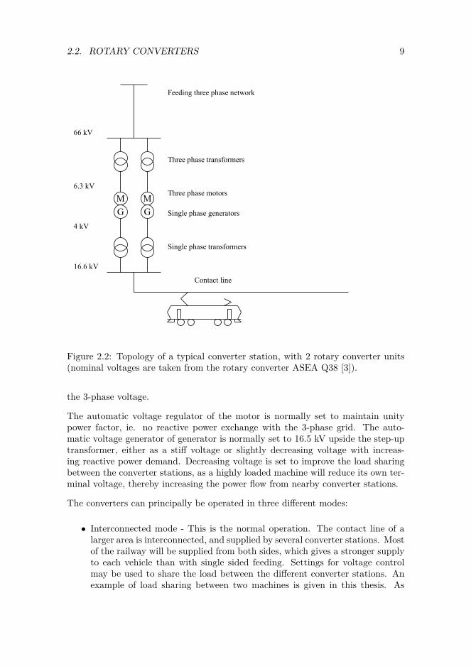
The converter units are normally installed in converter stations with 2 or 3 units,with a size per unit ranging from 3 to 10 MVA. The units are connected anddisconnected depending on the load situation to reduce losses. A typical topologyof a converter station is shown in figure 2.2. Each unit has a separate transformeron both the 3-phase and single phase side. The 3-phase side is connected to thegrid at 11-130 kV, while the single phase transformer is connected to the contactline. Two converter stations are also connected to the 55 kV high voltage line [2].
Both the motor and generator have brushless AC or DC excitation machines. Thesingle phase generator has damper windings, while the 3-phase motor has none.
2.2.1 Operation of Rotary Converters
The operation of synchronous - synchronous converters is mainly governed by twoaspects. First, the position of the field windings and thereby the angle of theinternal voltages of the motor and the generator are fixed to each other, as they aremechanically coupled. This could otherwise have been used to control torque andthereby real power. Secondly, the sum of real power input of the two machine mustbe zero in steady state (neglecting losses). Under transient conditions, deviationfrom zero sum will accelerate or decelerate the rotating mass.
As the real power in a synchronous machine is to large extent driven by the angledifference between the internal voltage and terminal voltage, the two machineswill find their respective angles giving equilibrium between incoming and outgoingpower. In other words, if the terminal voltage of the single phase side is laggingthe terminal voltage of the 3-phase side, power will flow from the 3-phase to thesingle phase side. During regeneration, power will flow from the single phase tothe 3-phase side, requiring the voltage angle on the single phase side to be leading
2.2. ROTARY CONVERTERS 9
MG
Contact line
Single phase transformers
Single phase generators
Three phase motors
Three phase transformers
Feeding three phase network
66 kV
6.3 kV
4 kV
16.6 kV
MG
Figure 2.2: Topology of a typical converter station, with 2 rotary converter units(nominal voltages are taken from the rotary converter ASEA Q38 [3]).
the 3-phase voltage.
The automatic voltage regulator of the motor is normally set to maintain unitypower factor, ie. no reactive power exchange with the 3-phase grid. The auto-matic voltage generator of generator is normally set to 16.5 kV upside the step-uptransformer, either as a stiff voltage or slightly decreasing voltage with increas-ing reactive power demand. Decreasing voltage is set to improve the load sharingbetween the converter stations, as a highly loaded machine will reduce its own ter-minal voltage, thereby increasing the power flow from nearby converter stations.
The converters can principally be operated in three different modes:
• Interconnected mode - This is the normal operation. The contact line of alarger area is interconnected, and supplied by several converter stations. Mostof the railway will be supplied from both sides, which gives a stronger supplyto each vehicle than with single sided feeding. Settings for voltage controlmay be used to share the load between the different converter stations. Anexample of load sharing between two machines is given in this thesis. As

10 CHAPTER 2. ELECTRIC TRACTION POWER SYSTEMS
this operation gives a relatively strong grid, stability is normally a smallerconcern.
• Islanded mode - Due to maintenance and fault situations, the contact lineis sectioned, which may leave a line section to be supplied from only oneconverter station. A long line section supplied from one end is the casenormally giving the weakest grid seen from the vehicle, and in which stabilitymay be problematic. This is the case chosen for stability analysis in thisthesis. The Norwegian National Rail Administration requires a vehicle to becapable of stable operation at a single fed line up to 60 km long [2]. Loadsharing is of course not an issue, as the entire section is supplied from oneconverter station.
• Reactive compensation mode - A synchronous machine may be used for volt-age control, only producing or consuming reactive power, without a mechan-ical load or prime mover. This mode is seldom used, and is not treated anyfurther.
2.3 Modern Electrical Rail Vehicles
The development of high performance power electronics and microcomputers allowsthe use of compact and robust asynchronous motors for traction of rail vehicles.These vehicles with power electronics, asynchronous motors and computer basedcontrol systems are often called modern or advanced electric rail vehicles. Otherdescriptions may be "inverter locomotive", "4 quadrant converter vehicle" or "asyn-chronous motor vehicle".
The main components of the modern electric rail vehicle is shown in figure 2.3.There is a step-down transformer, two four-quadrant converters connected by a DClink and asynchronous traction motors. The motor side converter is three-phase,supplying the asynchronous traction motors with variable voltage and frequency.The line side converter is single-phase, and controls the power flow between thegrid and the DC-link, depending on the power of the motor side converter.
Seen from the grid, the vehicle appears as a controllable voltage source behind theimpedance of the filter and the transformer.

2.3. MODERN ELECTRICAL RAIL VEHICLES 11
1~ =
= 3~
Contact line
Current collector
Return current in rails
Single phase line-side transformer
Line side converter
3-phase motor-side converter
DC-link
3-phase induction motor
Control system
Figure 2.3: The main components of a modern electrical rail vehicle
A sketch of the converter is shown in figure 2.4. The switching elements may bethyristors with quenching circuits, gate turn-off (GTO) thyristors or insulated gatebipolar transistors (IGBTs). The maximum internal voltage of the converter islimited by the DC-link voltage. The maximum current is limited by the thermallimit of the switches. Within these limitations, every current and correspondingreal and reactive powers are in principle possible. The real power is given by thetractive work to be done, leaving the reactive power to be controlled for otherpurposes [3].
As with the rotary converters, one side of the converter is single phase, giving aninstantaneous power pulsating with twice the fundamental frequency. The mainpurpose of the DC-link capacitor is to store energy in the DC-link, absorbing thepower pulsations and providing a constant power for the motor side converter.Filters may be included to reduce the harmonics of the DC-link voltage, shown infigure 2.4 as an RCL branch.

12 CHAPTER 2. ELECTRIC TRACTION POWER SYSTEMS
M~
Single phase line-side converter
DC-link 3-phase motor-side converter
3-phase induction motor
Figure 2.4: Simplified main circuit of a modern electrical rail vehicle
2.3.1 Operation
The main purpose of the circuit shown in figure 2.4 is to provide the tractionmotors the required power for the train’s propulsion. The traction motors arefed with variable voltage and frequency, depending on speed and required torque.When reducing speed or to maintain speed when driving downhill, the motors maybe operated as generators, braking the train. The power is fed back to the overheadline, to be used by other trains or fed back to the public grid, so-called regenerativebraking. Electric motor drives have a high efficiency, which causes the electric realpower to follow the mechanic power closely both during traction and regeneration.During transient conditions, a power unbalance may occur, charging or dischargingthe DC-link capacitor.
Real and reactive power may be controlled independently by controlling the internalvoltage magnitude and angle of the line side converter. Both real and reactivepower may be used to control the line voltage, improving stability and protectingthe system from voltage collapse. The vehicle’s response to varying line voltagemay be controlled by settings of the control system.
Generally, reactive power will be fed into the grid when consuming real power(traction) if this is needed to increase the line voltage. Similarly, reactive powermay be consumed during regenerative braking to prevent an unacceptable voltagerise.
For moderate power or in a strong network, the real power will normally be keptconstant at the level set by the driver, so that a voltage increase results in a current

2.3. MODERN ELECTRICAL RAIL VEHICLES 13
decrease. In this operation, the motor side converter appears as a constant powerDC load at the DC-link. The line side converter should supply or feed back thereal power required to keep the DC-link voltage Ud constant.
To distribute power between vehicles and protect a weak network from voltagecollapse, regulations require a reduction of vehicle’s main current at low voltage,which will limit the power. When available power is limited, this will limit thetractive effort at higher speeds. However, at start-up and low speed, the full tractiveforce is normally available regardless of line voltage [4].
An example of the steady state characteristics of a real vehicle is shown in thesummary of the fall project, in figure 3.5 and 3.9.

14 CHAPTER 2. ELECTRIC TRACTION POWER SYSTEMS
Chapter 3
Summary of Fall Project2010
A project with title "Active Control of Reactive Power in a Modern Electrical RailVehicle" [5] was done in the fall semester 2010, as a preliminary project for thisthesis. Two new control schemes were proposed for traction, while one new controlscheme was proposed for regenerative braking.
The control schemes proposed were implemented in a train model for traffic sim-ulation by SIMPOW/TracFeed, and evaluated regarding driving time and energyconsumption.
3.1 Research Objectives and Limitations
3.1.1 Research Questions
• Which use of reactive power allows the maximum power to be transferred tothe vehicle, within the technical and formal limitations that apply?
• When desired power is less than the possible transmission capacity (operatingin a strong grid or at moderate power), how can reactive power be used tominimize losses?
• How should reactive power be used during regenerative braking, to ensurereal power is not limited due to unacceptable voltage rise.
Simulations will be used to investigate the effects of reactive power control, withrespect to increased transmission capacity, reduced driving times, reduced losses
15

16 CHAPTER 3. SUMMARY OF FALL PROJECT 2010
and increased amount of energy fed back to the grid during braking.
Transmission capacity and loss are both electrical quantities which can be includedin an objective function for optimization, but simulations are required to find therelation between increased transmission capacity and reduced driving time. As theobjectives are reduced driving time and reduced losses, there are one optimizationfunction for power transfer, and another one for loss, simply saying that reducingdriving time has higher priority than reducing losses. However, to enable somecomparison, the different simulation results are compared with respect to energycosts vs. value of reduced driving time.
3.1.2 Applicable Regulations
The following regulations bring about limitations or constraints which the proposedcontrol schemes must comply with.
Permitted Voltages - EN:50163:2004
Electric railways in Norway are subject to the European standard EN50163:2004[7], which limits allowed voltages at the supply point to the train. The powerconsumed or fed back by the vehicle shall be limited to ensure that these voltagesare not exceeded. A summary of the voltages are given in table 3.1. The standardalso specifies permitted interval of temporary voltages. As the power consumptionshows large variations, the voltage is allowed to vary relatively much compared toother power systems; 0.8 - 1.15 pu. is allowed permanently.
Table 3.1: Allowed voltages according to EN50163:2004Lowest Lowest Nominal Highest Highest
non-permanent permanent voltage permanent non-permanentvoltage Umin2 voltage Umin2 Un voltage Umax1 voltage Umax2
11000 V 12000 V 15000 V 17250 V 18000 V
Current Limitation - EN:50388:2005
The power limitations to ensure permitted voltages are not exceed are defined inthe European standard EN50388:2005 [8]. The vehicle is permitted to draw itsnominal current at 14.25 kV (0.95 pu) and above. Below 14.25 kV, the tractioncurrent is to be ramped down linearly reaching zero at 11 kV (0.733 pu). It isthe magnitude of the current being limited, i.e. the real power for a given voltagemay vary depending on the power factor used. The limitation applies to traction

3.1. RESEARCH OBJECTIVES AND LIMITATIONS 17
current only, not current for auxiliary power. The current limitation is shown infigure 3.1, together with the same limitation expressed as appearent power.
11 12 13 14 15 16 17 180
0.2
0.4
0.6
0.8
1
1.2
Voltage [kV]
Tra
ctio
n cu
rren
t [pu
]
11 12 13 14 15 16 17 180
0.2
0.4
0.6
0.8
1
1.2
App
eare
nt p
ower
[pu]
Figure 3.1: The limitation of traction current according to EN50388:2005, repre-sented as current and appearent power as function of voltage. This figure does notapply for regenerative braking
Regenerative braking is not limited at low voltage, but is not permitted at linevoltage above Umax2 = 18 kV. No ramp down is specified, but stability requirementsshall be fulfilled.
Permitted Power Factor
Permitted power factors for new vehicles are defined in the requirements to rollingstock by the Norwegian National Rail Administration [2], shown in figure 3.2.Power factor is defined for the fundamental frequency, not the total RMS-values.The Norwegian requirements regarding power factor follow EN50388:2005 with mi-nor exceptions. This permits vehicles to use reactive power to control line voltage;using capacitive power factor during traction at low voltage, and inductive powerfactor during regeneration at high voltages. It is though required that stability ismaintained.

18 CHAPTER 3. SUMMARY OF FALL PROJECT 2010
Figure 3.2: Allowed power factor for the fundamental during traction and braking[2].
3.2 Control Schemes Proposed
The control schemes below are found for the following assumptions:
• The electric traction power system consists of overhead line with an impedanceof (0.19+ j0.21)Ω/km. The system is fed by one or more voltage stiff sourcesof 16.5 kV with the same voltage angle. This system may be transformed intoa Thevenin equivalent, with a Thevenin voltage of 16.5 kV and a Theveninimpedance Zth = leq · (0.19 + j0.21)Ω/km. leq indicates the equivalent linelength, i.e. the Thevenin impedance has the same impedance as a line withlength leq.
• The rated electric power of the load (a modern electrical rail vehicle) is 6.364MW and a rated voltage of 15 kV, giving a nominal current of 424.2 A.
• Auxillary power is neglected.

3.2. CONTROL SCHEMES PROPOSED 19
3.2.1 Traction
Minimum loss
The "minimum loss" control scheme is calculated to obtain the lowest line loss fora given power. As line loss at a given network configuration is only depending onthe current magnitude (Ploss = I2 · R), the lowest loss is obtained by keeping thecurrent magnitude as low as possible. When fed from a constant voltage source,the lowest current for a given power is obtained with unity power factor at thepoint with constant voltage, the feeding point. When the feeding voltage and X/Rratio or impedance angle θZline of the line is known, the load angle φ at the load isa function of the voltage at the load, equation 3.1. U1 is the voltage at the feedingpoint, assumed to be fixed, while U2 is the measured voltage at the vehicle’s currentcollector.
φ = θZline − sin−1 U1 sin θZlineU2
(3.1)
This mode of operation will imply feeding reactive power to cover the line loss(unity power factor at feeding point ⇒ all reactive power supplied from vehicle),which will increase the voltage at the load compared to running the load at unitypower factor. If the available power to the vehicle is limited due to voltage dropin a long line, this will also increase the available power. If neglecting the currentlimitation after EN50388 (section 3.1.2), allowing the vehicle to draw its nominalcurrent at any voltage, this is also the load angle giving maximum power to thevehicle.
Maximum power
A MATLAB script was made to find the maximum power possible within EN50388(section 3.1.2). At voltage at the vehicle above 14.25 kV, the load angle was thesame as for "minimum loss". At 14.25 kV and below, maximum power to the vehiclewas obtained by feeding back more reactive power than for "minimum loss". Thiswill increase the voltage and thereby make a higher current permitted. At quite asubstantial range of line lengths, the maximum power was obtained at the nominalcurrent, supplying reactive power to maintain voltage at 14.25 kV.
Comparison of Control Schemes
The control schemes proposed are compared with two reference cases, unity powerfactor at any voltage (no reactive power) and the reactive power control schemefrom a real locomotive [6]. The available power and within EN50388 and corre-sponding load angle, with the assumptions from section 3.2, is shown in figure 3.3,

20 CHAPTER 3. SUMMARY OF FALL PROJECT 2010
over a line length form 0 to 150 km. The corresponding line voltage and currentare shown in figure 3.4.
0 50 100 1500
2
4
6
Line length [km]
Ele
ctric
pow
er a
t veh
icle
[MW
]
Unity power factorFactory settingsMinimum lossMaximum power transfer
0 50 100 150−60
−40
−20
0
Line length [km]
Load
ang
le a
t veh
icle
[deg
rees
]
Unity power factorFactory settingsMinimum lossMaximum power transfer
Figure 3.3: Maximum possible power to the vehicle with different uses of reactivepower and its corresponding load angle, as a function of line length.
3.2. CONTROL SCHEMES PROPOSED 21
0 50 100 15012
13
14
15
16
Line length [km]
Line
vol
tage
[kV
]
0 50 100 1500
100
200
300
400
500
Line length [km]
Cur
rent
[A]
Unity power factorFactory settingsMinimum lossMaximum power transfer
Unity power factorFactory settingsMinimum lossMaximum power transfer
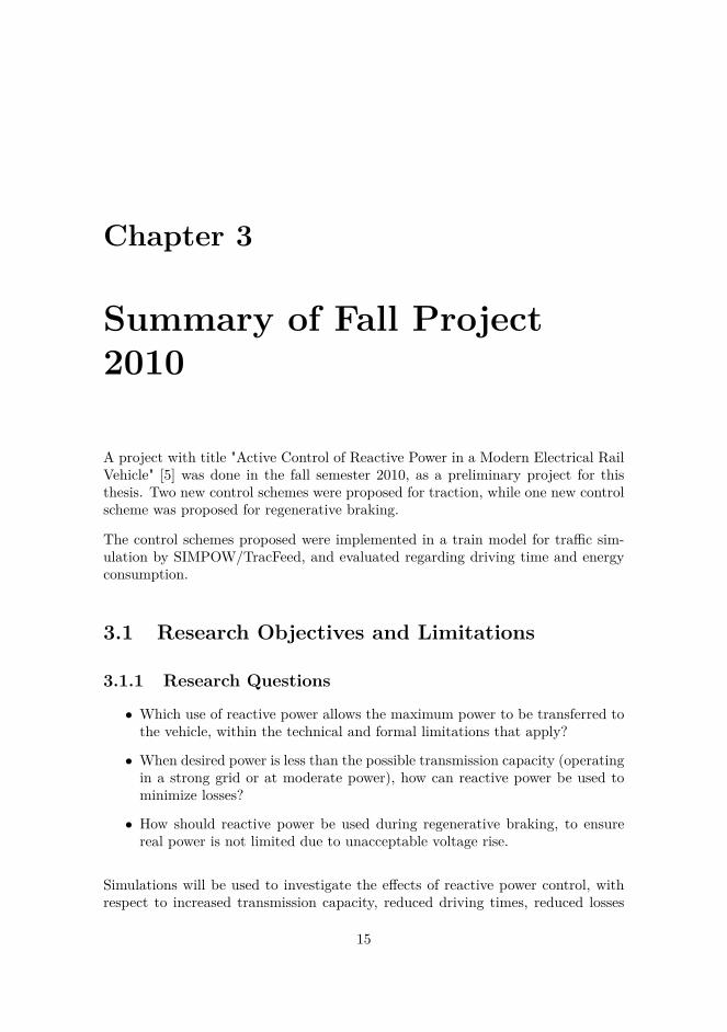
Figure 3.4: Line voltage and current when transferring maximum power with dif-ferent uses of reactive power, as a function of line length.
To be implemented in a SIMPOW/TracFeed simulation model, the permitted powerand load angle are to be given as functions of the line voltage. The data from figure3.3 and 3.4 are shown as functions of line voltage in figure 3.5. The current andapparent power for a given voltage are the same for all settings, as they are themaximum permitted within EN50388, figure 3.1.

22 CHAPTER 3. SUMMARY OF FALL PROJECT 2010
12 12.5 13 13.5 14 14.5 15 15.5 16 16.50
1
2
3
4
5
6
7
Line voltage [kV]
Pow
er [M
W]
12 12.5 13 13.5 14 14.5 15 15.5 16 16.5−60
−40
−20
0
Line voltage [kV]
Load
ang
le a
t veh
icle
[deg
rees
]
Unity power factorFactory settingsMinimum lossMaximum power transfer
Unity power factorFactory settingsMinimum lossMaximum power transfer
Figure 3.5: Power and load angle as functions of voltage.
Increased amount of reactive power fed into the line will, until a maximum, availablepower is the nose curve, with the real power as a function of the voltage, normallygiven for a constant power factor. The distance from the operating point to the tipof the nose curve (maximum power) is an indication for the margin from a voltagecollapse for a load with constant power characteristics. At unity power factor, thetip of the nose will occur at about half the no-load voltage, while at a capacitivepower factor, it will occur at higher voltage.

3.2. CONTROL SCHEMES PROPOSED 23
The nose curves for 30 km line length are shown in figure 3.6. The nose curvefor maximum power and minimum loss are identical, and indicate clearly a higheravailable power than unity power factor. All operating points have a large marginfrom the tip.
0 2 4 6 8 10 120
2
4
6
8
10
12
14
16
1830 km line
Real power at vehicle [MW]
Line
vol
tage
[kV
]
Unity power factorFactory settings − cos φ = 0.999Minimum loss − cos φ = 0.982Maximum power − cos φ = 0.982
Figure 3.6: Nose curves for 30 km line length with different power factors, powerfactors used at the operating points of the respective control schemes. The oper-ating points from figure 3.3 and 3.4 are marked with black circles.
24 CHAPTER 3. SUMMARY OF FALL PROJECT 2010
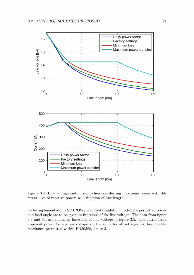
At 60 km, figure 3.7, the nose curves clearly show a lower available power thanat 30 km, regardless of power factor. Especially the curve for "maximum power"indicate that maximum power occurs at a higher voltage. All operating points havea significant margin to the tip.
0 2 4 6 8 10 120
2
4
6
8
10
12
14
16
1860 km line
Real power at vehicle [MW]
Line
vol
tage
[kV
]
Unity power factorFactory settings − cos φ = 0.987Minimum loss − cos φ = 0.954Maximum power − cos φ = 0.795
Figure 3.7: Nosecurves for 60 km line length with different power factors, power fac-tors used at the operating points of the respective control schemes. The operatingpoints from figure 3.3 and 3.4 are marked with black circles.
3.2. CONTROL SCHEMES PROPOSED 25
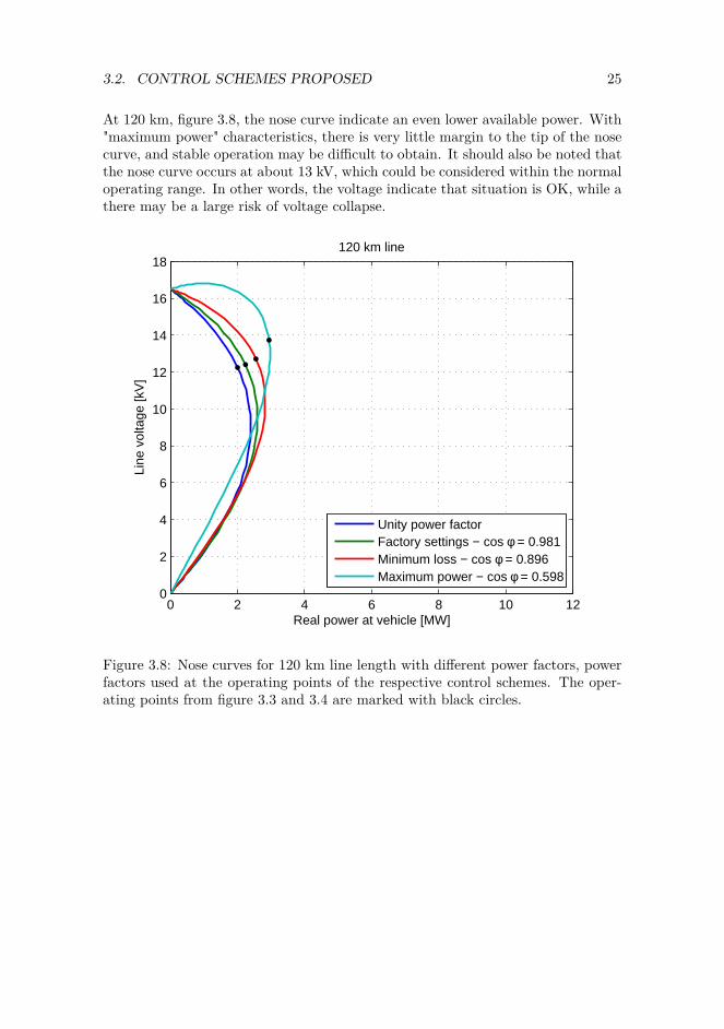
At 120 km, figure 3.8, the nose curve indicate an even lower available power. With"maximum power" characteristics, there is very little margin to the tip of the nosecurve, and stable operation may be difficult to obtain. It should also be noted thatthe nose curve occurs at about 13 kV, which could be considered within the normaloperating range. In other words, the voltage indicate that situation is OK, while athere may be a large risk of voltage collapse.
0 2 4 6 8 10 120
2
4
6
8
10
12
14
16
18120 km line
Real power at vehicle [MW]
Line
vol
tage
[kV
]
Unity power factorFactory settings − cos φ = 0.981Minimum loss − cos φ = 0.896Maximum power − cos φ = 0.598
Figure 3.8: Nose curves for 120 km line length with different power factors, powerfactors used at the operating points of the respective control schemes. The oper-ating points from figure 3.3 and 3.4 are marked with black circles.

26 CHAPTER 3. SUMMARY OF FALL PROJECT 2010
3.2.2 Regenerative Braking
The lowest losses for a given power, also during braking, are obtained when theconverter station is running at unity power factor, while the vehicle supplies allreactive power. This setting is not permitted during braking, as capacitive powerfactor is not allowed during regeneration, see figure 3.2. The closest possible wouldbe unity power factor.
However, as regenerative braking is not allowed at line voltages over 18 kV, thevoltage must be controlled, either by real or reactive power. To avoid limitingreal power, power factor should first be made sufficiently inductive to control thevoltage increase, before the real power is reduced. The settings are shown in figure3.9. With the factory setting, power factor is reduced from unity at 16.5 kV to 0.85inductive at 17 kV and above. Power is ramped down from full power up to 17 kVto 0 at 18 kV. For unity power factor, the real power ramp down is the same as forfactory settings.
A setting for reduced loss during regenerative braking is proposed. Full power atunity power factor is used up to 17.5 kV. From 17.5 kV to 17.75 kV, power factoris ramped down to 0.9. From 17.75 kV to 18 kV, the real power is ramped downfrom rated value to 0, see figure 3.9.

3.3. SIMULATION MODEL 27
15 15.5 16 16.5 17 17.5 180
2
4
6
Voltage [kV]
Line
pow
er r
egen
erat
ed [M
W]
Unity power factor and factory settingsReduced loss during regeneration
15 15.5 16 16.5 17 17.5 18−40
−20
0
Voltage [kV]
Load
ang
le [d
egre
es]
Unity power factorFactory settingsReduced loss during regeneration
Figure 3.9: Power limitation and reactive power control during braking.
3.3 Simulation Model
The control schemes proposed were implemented in a train model for SIMPOW/TracFeed,and simulated driving from Hønefoss to Nesbyen; a distance of 91.589 km. Powerlimitation and reactive power settings are described in figure 3.5 and 3.9. The trackdata and train data is also used in this thesis, shown in figure 4.7 and table A.1.The following combinations of settings for traction and braking were simulated:

28 CHAPTER 3. SUMMARY OF FALL PROJECT 2010
1 Unity power factor during both traction and regeneration
2 Factory settings; unity or capacitive during traction, inductive during regen-eration
3 Minimum losses; capacitive during traction, unity at regeneration
4 Minimum losses during traction (capacitive), factory settings (inductive) dur-ing regeneration
5 Minimum losses during traction (capacitive), settings for reduced loss duringregeneration (inductive)
6 Maximum power transfer during traction (capacitive), settings for reducedloss during regeneration (inductive)
The power system was modelled with two different configurations; with the contactline fed from the Nesbyen end and from both ends. The feeding was modelled asstiff voltage sources with the same angle and 16.5 kV. Single sided feeding fromNesbyen was used to give a weak power supply, in which available power at thelocomotive is limited, and increased power will give reduced driving time. Doublesided feeding was used to give a strong power supply, where power limitation wasnot an issue, but where reactive power control might reduce losses. All six trainmodels were simulated in both the weak and the strong configuration.
The value of reduced driving time of the train was found to 33100 NOK/hr. Thecost of electrical energy out from the converter station line was found to 0.4768NOK/kWh, while the value of regenerated energy fed back to the converter stationwas assumed to be 0.333 NOK/kWh.
3.4 Summary of Results
3.4.1 Single Fed Line - Weak Grid
Selected results from the simulations with a single fed line are shown in table 3.2.
3.4. SUMMARY OF RESULTS 29
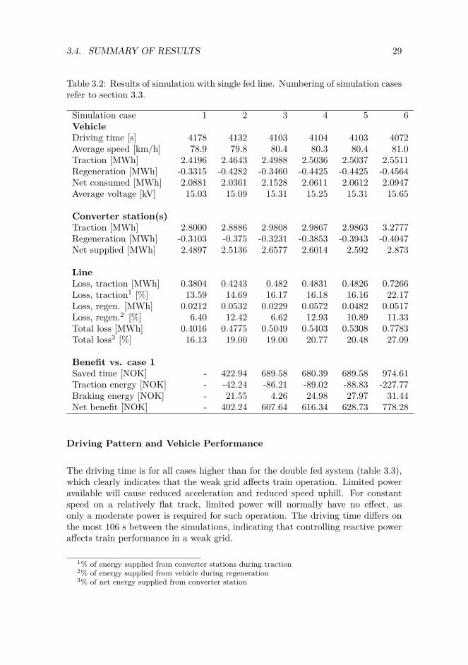
Table 3.2: Results of simulation with single fed line. Numbering of simulation casesrefer to section 3.3.
Simulation case 1 2 3 4 5 6VehicleDriving time [s] 4178 4132 4103 4104 4103 4072Average speed [km/h] 78.9 79.8 80.4 80.3 80.4 81.0Traction [MWh] 2.4196 2.4643 2.4988 2.5036 2.5037 2.5511Regeneration [MWh] -0.3315 -0.4282 -0.3460 -0.4425 -0.4425 -0.4564Net consumed [MWh] 2.0881 2.0361 2.1528 2.0611 2.0612 2.0947Average voltage [kV] 15.03 15.09 15.31 15.25 15.31 15.65
Converter station(s)Traction [MWh] 2.8000 2.8886 2.9808 2.9867 2.9863 3.2777Regeneration [MWh] -0.3103 -0.375 -0.3231 -0.3853 -0.3943 -0.4047Net supplied [MWh] 2.4897 2.5136 2.6577 2.6014 2.592 2.873
LineLoss, traction [MWh] 0.3804 0.4243 0.482 0.4831 0.4826 0.7266Loss, traction1 [%] 13.59 14.69 16.17 16.18 16.16 22.17Loss, regen. [MWh] 0.0212 0.0532 0.0229 0.0572 0.0482 0.0517Loss, regen.2 [%] 6.40 12.42 6.62 12.93 10.89 11.33Total loss [MWh] 0.4016 0.4775 0.5049 0.5403 0.5308 0.7783Total loss3 [%] 16.13 19.00 19.00 20.77 20.48 27.09
Benefit vs. case 1Saved time [NOK] - 422.94 689.58 680.39 689.58 974.61Traction energy [NOK] - -42.24 -86.21 -89.02 -88.83 -227.77Braking energy [NOK] - 21.55 4.26 24.98 27.97 31.44Net benefit [NOK] - 402.24 607.64 616.34 628.73 778.28
Driving Pattern and Vehicle Performance
The driving time is for all cases higher than for the double fed system (table 3.3),which clearly indicates that the weak grid affects train operation. Limited poweravailable will cause reduced acceleration and reduced speed uphill. For constantspeed on a relatively flat track, limited power will normally have no effect, asonly a moderate power is required for such operation. The driving time differs onthe most 106 s between the simulations, indicating that controlling reactive poweraffects train performance in a weak grid.
1% of energy supplied from converter stations during traction2% of energy supplied from vehicle during regeneration3% of net energy supplied from converter station

30 CHAPTER 3. SUMMARY OF FALL PROJECT 2010
Traction
Higher acceleration and increased average speed causes only a moderate increaseof traction energy consumed by the vehicle. From the slowest (78.9 km/h) to thefastest (81.0 km/h), speed is increased by 2.7 %, while the energy consumed isincreased by 131.5 kWh or 5.4 %. The speed of fastest train is 1.5 % higher thanfor the train with factory settings.
Power at the vehicle is roughly proportional to the current, while line loss is pro-portional with to the current squared. To transfer a given amount of energy, thelowest losses are obtained at the lowest power possible, i.e. the transfer takes moretime. Higher acceleration and increased speed cause higher power transferred overshorter time, and the consequence is higher losses. From the slowest, case 1, to thefastest, case 6, the energy consumed is increased by 131.5 kWh, while the line lossduring traction is increased by 346.2 kWh.
Regenerative Braking
Case 1 and 3 use unity power factor during regenerative braking. The energyregenerated is about 100 kWh lower for these cases, compared to the cases 2, 4, 5and 6, which consume reactive power during regeneration to control line voltage.For cases 1 and 3, the voltage is not controlled by reactive power, which means thatreal power is limited to avoid unacceptably high voltage. The minor differences inthe energy regenerated between case 2, 4 and 5, and 6 are probably caused bydifferent driving pattern.
To limit the losses, the reactive power consumed should only be enough to limitthe voltage at an acceptable level. Excess use of reactive power will increase losses.The settings for reduced loss during regeneration accepts up to 17.5 kV beforereactive power is used to control voltage, while the factory settings starts usingreactive power at 16.5 kV. The effect can be shown by comparing case 4 (factorysettings during regeneration) and 5 (reduced loss during regeneration). The energyregenerated from the vehicle is the same, while the line loss during regeneration is 9kWh lower for case 5, a reduction of 19 %. The reduced losses are, however on thecost of higher deviation from the nominal voltage. Case 4 and 5 are identical duringtraction, but the average voltage is higher for case 5, which means the voltageduring regeneration is higher. Case 6 also uses settings for reduced loss duringregeneration, and obtains lower loss than case 4, for more energy transferred.

3.4. SUMMARY OF RESULTS 31
3.4.2 Double Fed Line - Strong grid
Selected results from the simulations with a double fed line are shown in table 3.3.The detailed results are not included in the appendix, as the weak grid resultsalready illustrate the trains’ performance on the full range of line lengths, from91 km to 0. The differences between the simulation cases are also smaller with astrong grid than a weak.
Table 3.3: Results of simulation with double fed line. Numbering of simulationcases refer to section 3.3.
Simulation case 1 2 3 4 5 6VehicleDriving time [s] 4030 4030 4030 4030 4030 4030Average speed [km/h] 81.8 81.8 81.8 81.8 81.8 81.8Traction [MWh] 2.6578 2.6553 2.6587 2.6620 2.6577 2.6615Regeneration [MWh] -0.4639 -0.5041 -0.4639 -0.5043 -0.5044 -0.5041Net consumed [MWh] 2.1939 2.1512 2.1948 2.1577 2.1533 2.1574Average voltage [kV] 16.12 16.10 16.16 16.13 16.17 16.16
Converter station(s)Traction [MWh] 2.7920 2.7892 2.7920 2.7951 2.7906 2.7946Regeneration [MWh] -0.4385 -0.4706 -0.4385 -0.4706 -0.4746 -0.4742Net supplied [MWh] 2.3535 2.3186 2.3535 2.3245 2.316 2.3204
LineLoss, traction [MWh] 0.1342 0.1339 0.1333 0.1331 0.1329 0.1331Loss, traction1 [%] 4.81 4.80 4.77 4.76 4.76 4.76Loss, regen. [MWh] 0.0254 0.0335 0.0254 0.0337 0.0298 0.0299Loss, regen.2 [%] 5.48 6.65 5.48 6.68 5.91 5.93Total loss [MWh] 0.1596 0.1674 0.1587 0.1668 0.1627 0.163Total loss3 [%] 6.78 7.22 6.74 7.18 7.03 7.02
Benefit vs. case 1Saved time [NOK] - 0 0 0 0 0Traction energy [NOK] - 1.34 0.00 -1.48 0.67 -1.24Braking energy [NOK] - 10.69 0.00 10.69 12.02 11.89Net benefit [NOK] - 12.02 0.00 9.21 12.69 10.65
1% of energy supplied from converter stations during traction2% of energy supplied from vehicle during regeneration3% of net energy supplied from converter station
32 CHAPTER 3. SUMMARY OF FALL PROJECT 2010
Driving Pattern and Vehicle Performance
The driving time is the same for all simulation cases, which indicates that thegrid configuration is strong enough, not to affect train performance significantly.The traction energy consumption at the vehicle is however slightly different, whichmay indicate differences in driving pattern causing less than 1 second difference indriving time.
Traction
The energy consumed at by the vehicle during traction differs only 6.7 kWh betweenthe different cases, 0.25 % of the energy consumed during traction. The loss duringtraction shows a somewhat higher difference, with the highest, case 1 having about1.3 kWh or 1 % higher loss than the lowest, case 5. Case 1 (unity) and 2 (factorysettings) have very similar losses, the same is for the cases 3, 4, 5 and 6.
Regenerative Braking
In the strong grid, the energy regenerated is about 40 kWh lower for cases 1 and3 (unity power factor during regeneration), compared to the cases 2, 4, 5 and 6,(consuming reactive power during regeneration). Cases 2 and 4 (factory settingsduring regeneration) have losses about 3-4 kWh higher than case 5 and 6 (reducedloss during regeneration), a reduction of loss during regeneration of 9-12 %.
Chapter 4
Load Sharing betweenRotary Converters
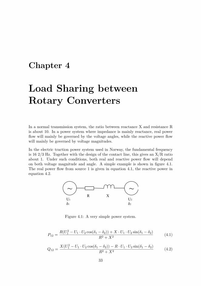
In a normal transmission system, the ratio between reactance X and resistance Ris about 10. In a power system where impedance is mainly reactance, real powerflow will mainly be governed by the voltage angles, while the reactive power flowwill mainly be governed by voltage magnitudes.
In the electric traction power system used in Norway, the fundamental frequencyis 16 2/3 Hz. Together with the design of the contact line, this gives an X/R ratioabout 1. Under such conditions, both real and reactive power flow will dependon both voltage magnitude and angle. A simple example is shown in figure 4.1.The real power flow from source 1 is given in equation 4.1, the reactive power inequation 4.2.
~ ~U1
δ1
U2
δ2
R X
Figure 4.1: A very simple power system.
P12 = R(U21 − U1 · U2 cos(δ1 − δ2)) +X · U1 · U2 sin(δ1 − δ2)
R2 +X2 (4.1)
Q12 = X(U21 − U1 · U2 cos(δ1 − δ2))−R · U1 · U2 sin(δ1 − δ2)
R2 +X2 (4.2)
33

34 CHAPTER 4. LOAD SHARING BETWEEN ROTARY CONVERTERS
The model shown in figure 4.1 may be used to determine the power flow betweentwo converter stations feeding each end of a contact line section. The voltagemagnitude can be controlled by the voltage regulators of the generators, either tobe kept constant or other characteristics, depending on what is desirable in thesystem. The voltage angle of each converter’s terminal voltage will mostly dependon the real power flow through the converter, and is little influenced by controllersettings. According to the Norwegian National Rail Administration [2], the angleof the single phase voltage will lag 36 at rated load with respect to the no loadangle.
If both converter stations are set to maintain constant 16.5 kV, and a load isplaced at the end of the line, close to the first converter station, this converterstation’s power angle will be lagging compared to its no load angle. This will causereal power to flow from the second converter station through the line, sharing thereal power power load between the two converter stations. However, accordingto equation 4.2, this situation will cause a flow of reactive power from the firstconverter station to the second through the line. This will increase the current,increasing real and reactive losses, and will cause both converter stations to run ata power factor significantly below unity. To reduce this reactive power flow, theconverter stations may be set to decrease their output voltage when loaded. Inthe Norwegian system, the voltage regulators are set either to a constant voltage,or decreasing voltage when supplying reactive power. This chapter will investigatehow the proposed control schemes for reactive power will affect load sharing andlosses in a power system fed by rotary converters, by a simulation in steady stateby SIMPOW, and a traffic simulation by SIMPOW/TracFeed.
4.1 Load Sharing in Steady State
4.1.1 Model Description
The system topology is shown in figure 4.2. Parameters are typical values givenby the Norwegian National Rail Administration [2]. The system consists of twoconverter stations, each with two converter units with a continuous power of 5.8MVA. Load flow analysis is done with both one and two converter units in operationin each converter station. Each converter unit has its own transformer both on the3-phase and single phase side. Converter and transformer data can be found inappendix A.3. The 3-phase grid is represented as a infinite bus of 66 kV, with lineimpedance giving a short circuit power at the 66 kV input to the converter stationsof 250 MVA. The 3-phase lines have a Z/R ratio of 4.
The load sharing is simulated with two different settings of the generators’ voltagecontrollers. One setting is constant 16.5 kV, the second setting is with a decreasingvoltage for increasing reactive power. The voltage decrease is set to 8 %, ie. theoutput voltage should be 0.92 pu = 15.18 kV when the generator supplies its
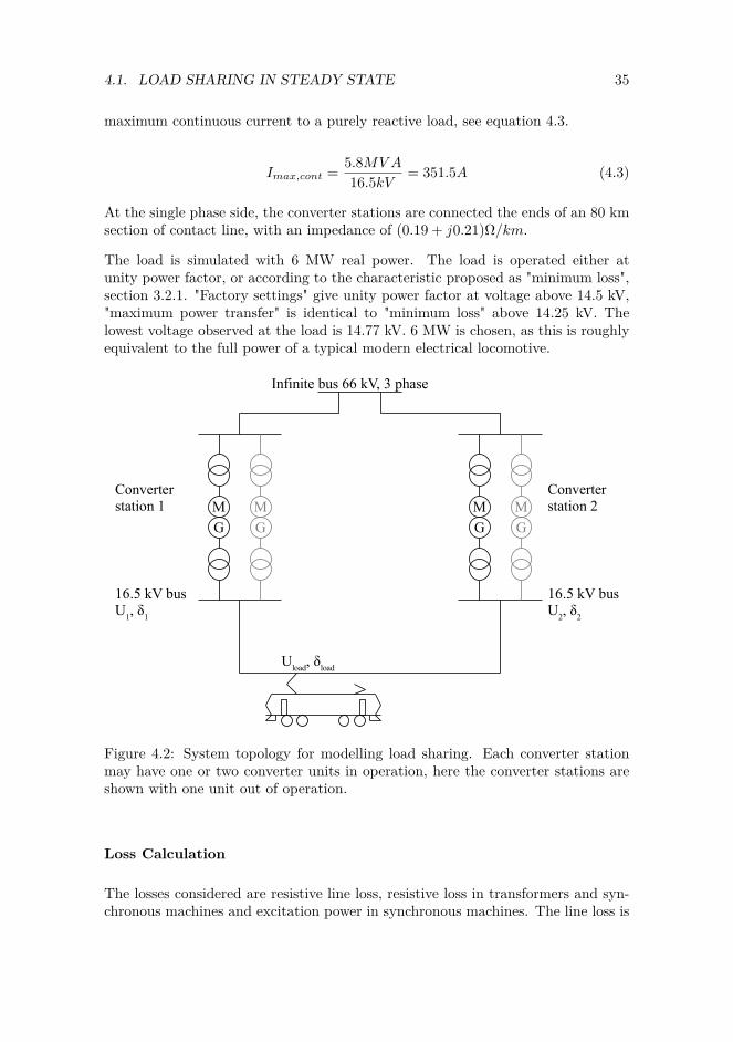
4.1. LOAD SHARING IN STEADY STATE 35
maximum continuous current to a purely reactive load, see equation 4.3.
Imax,cont = 5.8MVA
16.5kV = 351.5A (4.3)
At the single phase side, the converter stations are connected the ends of an 80 kmsection of contact line, with an impedance of (0.19 + j0.21)Ω/km.
The load is simulated with 6 MW real power. The load is operated either atunity power factor, or according to the characteristic proposed as "minimum loss",section 3.2.1. "Factory settings" give unity power factor at voltage above 14.5 kV,"maximum power transfer" is identical to "minimum loss" above 14.25 kV. Thelowest voltage observed at the load is 14.77 kV. 6 MW is chosen, as this is roughlyequivalent to the full power of a typical modern electrical locomotive.
Converter station 1
Converter station 2
Infinite bus 66 kV, 3 phase
16.5 kV busU1, δ1
16.5 kV busU2, δ2
Uload, δload
MG
MG
MG
MG
Figure 4.2: System topology for modelling load sharing. Each converter stationmay have one or two converter units in operation, here the converter stations areshown with one unit out of operation.
Loss Calculation
The losses considered are resistive line loss, resistive loss in transformers and syn-chronous machines and excitation power in synchronous machines. The line loss is

36 CHAPTER 4. LOAD SHARING BETWEEN ROTARY CONVERTERS
found as the difference of real power into the contact line and out of the contactline. The resistive loss in transformers and synchronous machines is found as thedifference between real power at the 3-phase input and real power at the singlephase output of the converter station. The excitation power is found from theexcitation current from the simulation IF,pu in pu, the field winding resistance RFand no-load field current IF0, by equation 4.4.
PF = I2F,pu · I2
F0 ·RF (4.4)
The loss in the field machines is neglected, as this is in the range of some tens ofwatts. Iron loss in transformers and synchronous machines is neglected, as theseare mostly voltage dependent and the voltage is nearly constant. Mechanical losses,such as friction and fans fixed to the converter shaft, are neglected, as these arespeed dependent and the speed is fixed at the synchronous speed. Auxiliary powerin the converter stations, such as cooling fans for transformers, is neglected as theload dependency is difficult to estimate. As most no-load losses are neglected,the results cannot be used for comparing the converter losses when running twoconverter units vs. one. Losses in the 3-phase grid are not considered, as this willmostly depend on the load and operation of the 3-phase grid, which is not includedin this model.
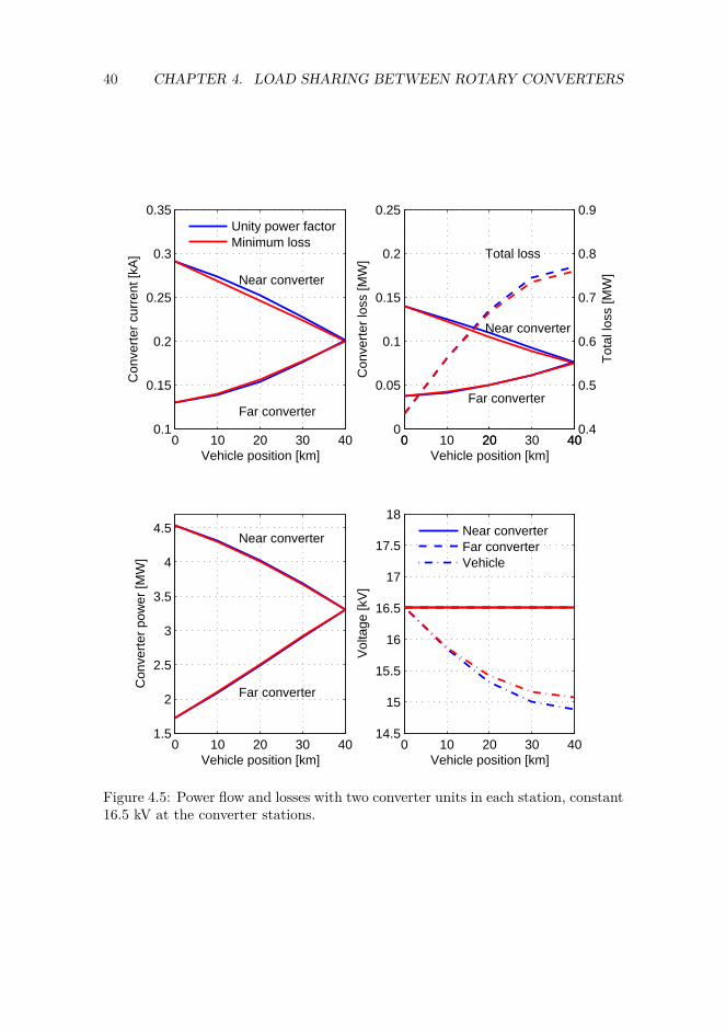
4.1.2 Results
Four different configurations of the power supply are simulated, with one and twoconverter units in each converter station, and with constant 16.5 kV and 8 % de-creasing voltage characteristics. As the system is symmetrical around the midpoint,the system is simulated with the load located outside one converter station (0+80km), and in 10 km steps to the midpoint (40+40 km).
The effect of changing from unity power factor to "minimum loss" is shown in figure4.3 to 4.6, with respect to sharing of real power load, sharing of current load, lossin the most highly loaded converter station and total loss (both converter stationsand single phase line). The location of the load in the graphs is given in km fromthe closest converter station.
The four cases simulated all show the same basic effects. In the cases with constant16.5 kV from the converter stations, the "minimum loss" settings has no effect whenthe vehicle is located at the converter station, as the "minimum loss" settings giveunity power factor at 16.5 kV. The effect on load distribution is largest in thearea around half way from the end to the midpoint of the line, about 20 km fromthe nearest converter station. More even load distribution means lower load andlower losses in the converter station nearest to the load, increasing the marginfrom overloading the converter station. More even load distribution require morepower to be transferred from the furthest converter station through the longest linesection, which in some cases increase the total line losses.

4.1. LOAD SHARING IN STEADY STATE 37
"Minimum loss" gives equal or higher voltage, with the largest effect on the mid-point of the line, where voltage is increased by 190-290 V depending on number ofconverter units in operation and the settings of the automatic voltage regulators.
Table 4.1 shows the largest effect of controlling reactive power. The highest re-duction of current and real power at the most highly loaded converter station isobtained with the load 20 km from the nearest converter station. Reducing theload at the most highly loaded converter station will increase the margin fromoverloading the converter station, in other words enable higher power supplied tothe load. The "minimum loss" settings are intended to reduce line loss. This effectis most significant at the midpoint of the line, where the line loss is highest.

38 CHAPTER 4. LOAD SHARING BETWEEN ROTARY CONVERTERS
0 10 20 30 400.1
0.15
0.2
0.25
0.3
0.35
Vehicle position [km]
Con
vert
er c
urre
nt [k
A]
Near converter
Far converter
Unity power factorMinimum loss
0 10 20 30 401.5
2
2.5
3
3.5
4
4.5
Vehicle position [km]
Con
vert
er p
ower
[MW
]
Near converter
Far converter
0 10 20 30 400
0.05
0.1
0.15
0.2
0.25
Vehicle position [km]
Con
vert
er lo
ss [M
W]
Near converter
Far converter
Total loss
0 20 400.4
0.5
0.6
0.7
0.8
0.9
Tot
al lo
ss [M
W]
0 10 20 30 4014.5
15
15.5
16
16.5
17
17.5
18
Vehicle position [km]
Vol
tage
[kV
]
Near converterFar converterVehicle
Figure 4.3: Power flow and losses with one converter unit in each station, constant16.5 kV at the converter stations.

4.1. LOAD SHARING IN STEADY STATE 39
0 10 20 30 400.1
0.15
0.2
0.25
0.3
0.35
Vehicle position [km]
Con
vert
er c
urre
nt [k
A]
Near converter
Far converter
Unity power factorMinimum loss
0 10 20 30 401.5
2
2.5
3
3.5
4
4.5
Vehicle position [km]
Con
vert
er p
ower
[MW
] Near converter
Far converter
0 10 20 30 400
0.05
0.1
0.15
0.2
0.25
Vehicle position [km]
Con
vert
er lo
ss [M
W]
Near converter
Far converter
Total loss
0 20 400.4
0.5
0.6
0.7
0.8
0.9
Tot
al lo
ss [M
W]
0 10 20 30 4014.5
15
15.5
16
16.5
17
17.5
18
Vehicle position [km]
Vol
tage
[kV
]
Near converterFar converterVehicle
Figure 4.4: Power flow and losses with one converter unit in each station, 8 %decreasing voltage at the converter stations.
40 CHAPTER 4. LOAD SHARING BETWEEN ROTARY CONVERTERS
0 10 20 30 400.1
0.15
0.2
0.25
0.3
0.35
Vehicle position [km]
Con
vert
er c
urre
nt [k
A]
Near converter
Far converter
Unity power factorMinimum loss
0 10 20 30 401.5
2
2.5
3
3.5
4
4.5
Vehicle position [km]
Con
vert
er p
ower
[MW
]
Near converter
Far converter
0 10 20 30 400
0.05
0.1
0.15
0.2
0.25
Vehicle position [km]
Con
vert
er lo
ss [M
W]
Near converter
Far converter
Total loss
0 20 400.4
0.5
0.6
0.7
0.8
0.9
Tot
al lo
ss [M
W]
0 10 20 30 4014.5
15
15.5
16
16.5
17
17.5
18
Vehicle position [km]
Vol
tage
[kV
]
Near converterFar converterVehicle
Figure 4.5: Power flow and losses with two converter units in each station, constant16.5 kV at the converter stations.

4.1. LOAD SHARING IN STEADY STATE 41
0 10 20 30 400.1
0.15
0.2
0.25
0.3
0.35
Vehicle position [km]
Con
vert
er c
urre
nt [k
A]
Near converter
Far converter
Unity power factorMinimum loss
0 10 20 30 401.5
2
2.5
3
3.5
4
4.5
Vehicle position [km]
Con
vert
er p
ower
[MW
]
Near converter
Far converter
0 10 20 30 400
0.05
0.1
0.15
0.2
0.25
Vehicle position [km]
Con
vert
er lo
ss [M
W]
Near converter
Far converter
Total loss
0 20 400.4
0.5
0.6
0.7
0.8
0.9
Tot
al lo
ss [M
W]
0 10 20 30 4014.5
15
15.5
16
16.5
17
17.5
18
Vehicle position [km]
Vol
tage
[kV
]
Near converterFar converterVehicle
Figure 4.6: Power flow and losses with two converter units in each station, 8 %decreasing voltage at the converter stations.
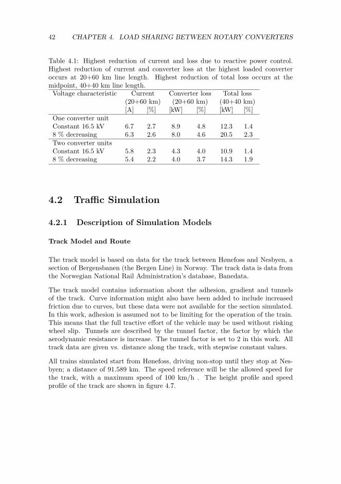
42 CHAPTER 4. LOAD SHARING BETWEEN ROTARY CONVERTERS
Table 4.1: Highest reduction of current and loss due to reactive power control.Highest reduction of current and converter loss at the highest loaded converteroccurs at 20+60 km line length. Highest reduction of total loss occurs at themidpoint, 40+40 km line length.Voltage characteristic Current Converter loss Total loss
(20+60 km) (20+60 km) (40+40 km)[A] [%] [kW] [%] [kW] [%]
One converter unitConstant 16.5 kV 6.7 2.7 8.9 4.8 12.3 1.48 % decreasing 6.3 2.6 8.0 4.6 20.5 2.3Two converter unitsConstant 16.5 kV 5.8 2.3 4.3 4.0 10.9 1.48 % decreasing 5.4 2.2 4.0 3.7 14.3 1.9
4.2 Traffic Simulation
4.2.1 Description of Simulation Models
Track Model and Route
The track model is based on data for the track between Hønefoss and Nesbyen, asection of Bergensbanen (the Bergen Line) in Norway. The track data is data fromthe Norwegian National Rail Administration’s database, Banedata.
The track model contains information about the adhesion, gradient and tunnelsof the track. Curve information might also have been added to include increasedfriction due to curves, but these data were not available for the section simulated.In this work, adhesion is assumed not to be limiting for the operation of the train.This means that the full tractive effort of the vehicle may be used without riskingwheel slip. Tunnels are described by the tunnel factor, the factor by which theaerodynamic resistance is increase. The tunnel factor is set to 2 in this work. Alltrack data are given vs. distance along the track, with stepwise constant values.
All trains simulated start from Hønefoss, driving non-stop until they stop at Nes-byen; a distance of 91.589 km. The speed reference will be the allowed speed forthe track, with a maximum speed of 100 km/h . The height profile and speedprofile of the track are shown in figure 4.7.

4.2. TRAFFIC SIMULATION 43
0 10 20 30 40 50 60 70 80 90−20
0
20
40
60
80
100
120
140
Distance from Honefoss [km]
Alti
tude
ref
erre
d to
Hon
efos
s [m
]
0 10 20 30 40 50 60 70 80 90−20
0
20
40
60
80
100
120
140
Allo
wed
spe
ed [k
m/h
]
Figure 4.7: Heightprofile and allowed speed between Hønefoss and Nesbyen
Train Model
The train is intended to be a typical freight train in Norway, consisting of a singlelocomotive of 5.6 MW and 36 two-axle cars, giving a total train mass of 1000 t.The cars are a mix of open and closed cars. A real train would normally consist ofa mix of 2, 4 and 6-axle cars, but the total number of axles is realistic. Train datais given in table A.1.
Electrical Model
The electrical infrastructure model used is most aspects the same as described insection 4.1.1, shown in figure 4.2. One converter unit is used in each converterstation. The length of contact line is increased to 91.589 km, corresponding to thetrack model. The simulation is run with both constant 16.5 kV at the converterstations and 8 % decreasing voltage characteristics.
The power limitation of the vehicle by EN50388:2005 is not implemented in thesimulation model. Feeding reactive power into the overhead line will increase theline voltage, permitting a higher current and power. The "minimum loss" char-acteristics is intended to give the minimum loss for a given power, but increasedpower may though increase the loss. To avoid this effect, the trains are allowedto consume full power, 6.364 MW, over the voltage range occurring in the simu-
44 CHAPTER 4. LOAD SHARING BETWEEN ROTARY CONVERTERS
lations. Three different train models are used, with different settings for reactivepower during traction, see section 3.2.1. All models use factory settings for powerlimitation and reactive power characteristics during regeneration.
1. Unity power factor during traction, factory settings during regeneration
2. Factory settings
3. "Minimum loss" during traction, factory settings during regeneration
4.2.2 Results
Constant 16.5 kV
The results from the traffic simulations with constant 16.5 kV from the converterstations are shown in table 4.2. The results with unity power factor (case 1) andfactory settings (case 2) are very similar. The factory settings give unity powerfactor above 14.5 kV, and the voltage is above this almost all the time. This canbe seen form the reactive production from the vehicle, where case 2 has virtuallyno reactive production (0.0002 MVArh).
The converter losses at Hønefoss converter are reduced by 1.5 kWh from unity tominimum loss, while the losses at Nesbyen converter station is almost unaffected.This is probably because Hønefoss converter is the most heavily loaded, because ofthe uphill starting 15 km after departure from Hønefoss. In the load flow analysis,the "minimum loss" settings gave better distribution of load between the converterstations, which would decrease the load on Hønefoss. Lower total converter lossesindicate more even distribution of load, which reduces the risk of overloading theconverters.
The line loss is increased by the "minimum loss" settings, similar to the load anal-ysis, where both the real and the reactive power of the furthest converter stationincreased, increasing the line loss.

4.2. TRAFFIC SIMULATION 45
Table 4.2: Traffic simulation with constant 16.5 kV from converter stations. Thelast column shows the relative change from case 1 (unity power factor) to case 3("minimum loss").
Simulation case ChangeUnit 1 2 3 1 to 3 [%]
VehicleDriving time s 4030 4030 4029Traction energy MWh 2.6593 2.6541 2.6590 -0.01Energy regenerated MWh -0.5041 -0.5040 -0.5054 0.26Reactive consumption MVArh 0.1597 0.1616 0.1565 -2.00Reactive production MVArh 0.0001 -0.0002 -0.1655
Hønefoss converter stationMax current, 2 s kA 0.3147 0.3159 0.3141 -0.18Max current, 6 min kA 0.2231 0.2230 0.2164 -2.99Max current, 1 hr kA 0.1340 0.1337 0.1319 -1.55Loss during traction MWh 0.0465 0.0464 0.0454 -2.37Loss during regeneration MWh 0.0035 0.0034 0.0034 -2.86Excitation loss MWh 0.0125 0.0125 0.0122 -2.25Total converter loss MWh 0.0625 0.0623 0.0610 -2.37
Nesbyen converter stationMax current, 2 s kA 0.3033 0.3034 0.2978 -1.80Max current, 6 min kA 0.1613 0.1613 0.1588 -1.55Max current, 1 hr kA 0.1163 0.1164 0.1165 0.18Loss during traction MWh 0.0354 0.0355 0.0354 0.00Loss during regeneration MWh 0.0033 0.0032 0.0033 0.00Excitation loss MWh 0.0116 0.0116 0.0114 -1.68Total converter loss MWh 0.0503 0.0503 0.0501 -0.39
Contact lineLoss during traction MWh 0.1812 0.1815 0.1820 0.44Loss during regeneration MWh 0.0366 0.0361 0.0364 -0.55Total line loss MWh 0.2178 0.2176 0.2184 0.28
SystemTraction energy MWh 2.9224 2.9175 2.9218 -0.02Regeneration MWh -0.4607 -0.4613 -0.4623 0.35Net energy consumption MWh 2.4821 2.4766 2.4795 -0.11Total loss MWh 0.3307 0.3303 0.3296 -0.33

46 CHAPTER 4. LOAD SHARING BETWEEN ROTARY CONVERTERS
Decreasing Voltage Characteristics
The results from the traffic simulations with 8 % decreasing voltage characteristicsfrom the converter stations are shown in table 4.3. Decreasing voltage character-istics give lower losses than constant 16.5 kV in all components (excitation lossesin Nesbyen converter station are unchanged). The effect of reactive power con-trol at the vehicle shows the same tendency as for constant 16.5 kV; slightly lowerconverter losses, especially for Hønefoss converter station, and higher line losses.Lower total converter losses indicate more even distribution of load, which reducesthe risk of overloading the converters.

4.2. TRAFFIC SIMULATION 47
Table 4.3: Traffic simulation with 8 % decreasing voltage characteristics from con-verter stations. The last column shows the relative change from case 1 (unity powerfactor) to case 3 ("minimum loss").
Simulation case ChangeUnit 1 2 3 1 to 3 [%]
VehicleDriving time s 4030 4030 4029Traction energy MWh 2.6503 2.6515 2.6515 0.05Energy regenerated MWh -0.5031 -0.5034 -0.5057 0.52Reactive consumption MVArh 0.1355 0.1358 0.1317 -2.80Reactive production MVArh 0.0001 -0.0029 -0.1819
Hønefoss converter stationMax current, 2 s kA 0.3024 0.3024 0.2986 -1.23Max current, 6 min kA 0.2169 0.2171 0.2122 -2.17Max current, 1 hr kA 0.1311 0.1312 0.1296 -1.16Loss during traction MWh 0.0446 0.0447 0.0442 -0.90Loss during regeneration MWh 0.0032 0.0032 0.0030 -6.25Excitation loss MWh 0.0123 0.0123 0.0120 -2.47Total converter loss MWh 0.0601 0.0602 0.0592 -1.50
Nesbyen converter stationMax current, 2 s kA 0.2929 0.2926 0.2848 -2.77Max current, 6 min kA 0.1554 0.1548 0.1516 -2.41Max current, 1 hr kA 0.1146 0.1145 0.1139 -0.64Loss during traction MWh 0.0348 0.0347 0.0342 -1.72Loss during regeneration MWh 0.0031 0.0030 0.0033 6.45Excitation loss MWh 0.0116 0.0116 0.0114 -1.61Total converter loss MWh 0.0495 0.0493 0.0489 -1.18
Contact lineLoss during traction MWh 0.1797 0.1786 0.1840 2.39Loss during regeneration MWh 0.0350 0.0362 0.0315 -10.00Total line loss MWh 0.2147 0.2148 0.2155 0.37
SystemTraction energy MWh 2.9094 2.9095 2.9139 0.15Regeneration MWh -0.4618 -0.4610 -0.4679 1.32Net energy consumption MWh 2.4678 2.4687 2.4657 -0.08Total loss MWh 0.3243 0.3243 0.3236 -0.21

48 CHAPTER 4. LOAD SHARING BETWEEN ROTARY CONVERTERS
4.3 Discussion and Conclusion
4.3.1 Discussion
When the load is located near one end of the line, the settings "minimum loss"distributes load more evenly, reducing the load and the loss in the nearest converterstation. This is, however done at some cost. In a situation with a load close to oneend of the line section, reactive power will flow to the converter station furthestfrom the load. Feeding in more reactive power from the load will increase this flow.When also real power is distributed more evenly between the converter stations,this means both real and reactive power flow will increase between the load andthe most remote converter station, causing increased line loss. The "minimum loss"settings tend to reduce the loss of the closest converter station, while increasingthe line loss and the loss in the furthest converter station, in total giving a slightreduction of losses.
Sharing the load more evenly between the converter stations will reduce the loadon the most heavily loaded converter station, the converter station closest to beingoverloaded. This will increase the possible loading of the system before a converterstation is overloaded.
In a situation where the load is close to the midpoint of the line, load is sharedequally between the converter stations regardless of power factor of the load. Inthis situation, the "minimum loss" settings gives lower loss, without negative sideeffects.
In the traffic simulation, "minimum loss" gives higher line loss but smaller con-verter losses, giving a total of slightly lower losses. The converter losses are mainlyreduced on the most heavily loaded converter station, Hønefoss. Lower converterlosses indicate higher margin from overloading the converters. The overload limitof the converter stations is mainly determined by the allowed temperature in theconverters, and lower converter losses mean less heat produced inside the convert-ers.
Martinsen [9] describes how decreasing voltage characteristics depending on reac-tive power has small effect for modern locomotives, as they have a power factorclose to unity. A voltage characteristic with decreasing voltage depending on realpower load would probably give a more even load distribution between the con-verter stations for loads with unity or capacitive power factor. The topic of thisthesis is to investigate the consequences of the proposed settings for vehicles whenoperating at the existing infrastructure, not to find optimal settings of the converterstations, and this topic in not considered any further.

4.3. DISCUSSION AND CONCLUSION 49
4.3.2 Conclusion
Load Flow Simulation
The settings "minimum loss" tend to reduce the load on the closest, most heavilyloaded converter station, increasing the possible load of the system without over-loading the converters. However, these settings will in some cases increase the linelosses, as more power is to be transferred on a long line section from the furthestconverter station.
The minimum loss settings will reduce or keep the total losses unchanged, depend-ing on the position of the load, number of converters in operation and the settingsof the automatic voltage regulators. The largest effect is observed at the midpointof the line, where the total loss is reduced by 10.9 to 20.5 kW for a 6 MW load, areduction of 1.4 to 2.3 %.
The load of the highest loaded converter station will be reduced or kept unchanged,by distributing the load more evenly between the converter stations. The largesteffect is observed with the load 20 km from the nearest converter station. Depend-ing on the number of converters in operation and the settings of the automaticvoltage regulators, the current at highest loaded converter station is reduced by5.4 to 6.7 A for a 6 MW load, or 2.2 to 2.7 %. The loss in the converter station,which is the heat which may cause overload, is reduced by 4 to 8.9 kW, or 3.7 to4.8 %.
"Minimum loss" gives equal or higher voltage, with the largest effect when the vehi-cle is at the midpoint of the line, where voltage is increased by 190-290 V dependingon number of converter units in operation and the settings of the automatic voltageregulators.
Traffic Simulation
In the traffic simulation, the converter losses in the highest loaded converter wasreduced by 1.5 kWh or 2.4 % with constant voltage characteristics, and 0.9 kWh or1.5 % with 8 % decreasing characteristics, when changing from unity power factorto "minimum loss" settings of the load. The highest current occurring is reducedby 0-3 %.
The total losses are reduced by 1.1 kWh or 0.33 % with constant voltage character-istics, and 0.7 kWh or 0.21 % with 8 % decreasing characteristics, when changingfrom unity power factor to "minimum loss" settings of the load.

50 CHAPTER 4. LOAD SHARING BETWEEN ROTARY CONVERTERS
4.3.3 Further Work
The "minimum loss" settings are calculated to give the minimum loss under theassumption that the system is fed by voltage sources with the same voltage angleand magnitude. This assumption is not valid in the real system fed by more thanone converter station, where the voltage angles of the converter stations have alarge load dependency. It is thereby not given that these are the settings givingthe lowest loss in the real system. Thus, further investigation of the following is ofinterest:
• Finding a control scheme for reactive power reducing the losses and increas-ing the capacity based on a real system, including the characteristics of athe converter stations. An optimization will probably give different settingsdepending on the location in the grid (distance to and characteristics of therespective converter stations). When deciding the characteristics to be im-plemented in a vehicle, this should be taken into consideration giving a goodoverall performance at any location and grid configuration which is likely tooccur.
• Finding optimal settings for the voltage characteristics of the converter sta-tions. These settings will probably give an output voltage depending on bothreal and reactive power.
Chapter 5
Stability and Effect ofReactive Power
5.1 Simulation Model
The simulation model used is with minor modifications the model developed byDanielsen in [3]. Also methodology, symbols and terminology are to large extentthe same as used by Danielsen.
The model represents a universal electrical locomotive, 60 km overhead line, aconverter station with one rotary converter unit and an overlying 3-phase grid. Thelocomotive is a modern electrical rail vehicle, which allows indepedant control ofreal and reactive power. Such a system is shown in figure 2.2; with the modificationthat the figure indicates two converter units, for stability analysis only one is used.The system parameters can be found in appendix A.
The model developed by Danielsen gives unity power factor in steady state at thevehicle’s current collector. To investigate the effect of reactive power, the modelis modified to allow control of reactive power. The model allows two modes ofoperation, constant and voltage dependant power factor.
5.1.1 Vehicle Control Structure
The main circuit of the vehicle is modelled with the line transformer, one PWMconverter and one DC-link. The motor side converter is not modelled, but replacedwith a load on the DC-link. Two shunts are present at the DC-link, one capacitorand one RCL series branch. The RCL branch is a filter tuned to 33.4 Hz.
51

52 CHAPTER 5. STABILITY AND EFFECT OF REACTIVE POWER
SOGIαβ
dq
uα1
uβ1
SOGIαβ
dq
iα
iβ
PLL
CC
QC POD
dq
αβ
VC
ud1
uq1
id
iq
1~
PWM =
udcref=1
Transformer
Xt Rt
udc idcm
tan(φ)ref
θPLL
θPLL
udref
uqref
uacref
ud1
uq1
iacuac1
Cd Filter Motor
AC current measurement
AC voltage measurementiqPOD
uac
idref
Figure 5.1: The control system of the line side converter.
The control of the line side converter is modelled in a rotating reference frame, alsocalled vector control or dq-control, after the direct and quadrature axis. The signalflow is shown in figure 5.1. Lowercase letters indicate instantaneous values, bothfor real AC and DC values and when transformed into the d- and q-components.Uppercase letters indicate RMS values.
The d-axis reference is the voltage at the vehicle’s current collector. This is thevehicle’s interface with the power system, and regulations regarding eg. powerfactor or current limitation generally consider voltage and current at this point.

5.1. SIMULATION MODEL 53
Real power is thereby controlled by d-axis current, while reactive power is controlledby q-axis current.
5.1.2 DC-link Voltage Controller - VC
The main control objective of the converter is to keep the DC link voltage constant.The DC-link voltage udc is measured, and fed into the voltage controller. Thevoltage controller, figure 5.2, is based in a PI controller, controlling the d-axiscurrent, in other words real power into the vehicle and the vehicle’s DC-link. TheDC-link voltage reference is set to 1 pu.
The motor current is also measured and fed forward to give a faster responseto load changes. Without measuring the motor current, increased motor currentwould cause a reduced DC-link voltage, which then should be compensated bythe voltage controller, but with the feed-forward, this input is sent directly to thecurrent controller.
KpVC
1TiVC s
+
+
x2
+
+ -
udcPOD
udcref
udc_fil
LPF
udc
× ÷
LPF
idcm
idcm_fil
idcref
udc_fil
ud1
idref
PI controller
Figure 5.2: Voltage controller (VC).
5.1.3 AC Measurements
The instantaneous values of the line voltage and current are measured. In a 3-phase system, the instantaneous values can easily be converted into two orthogonal
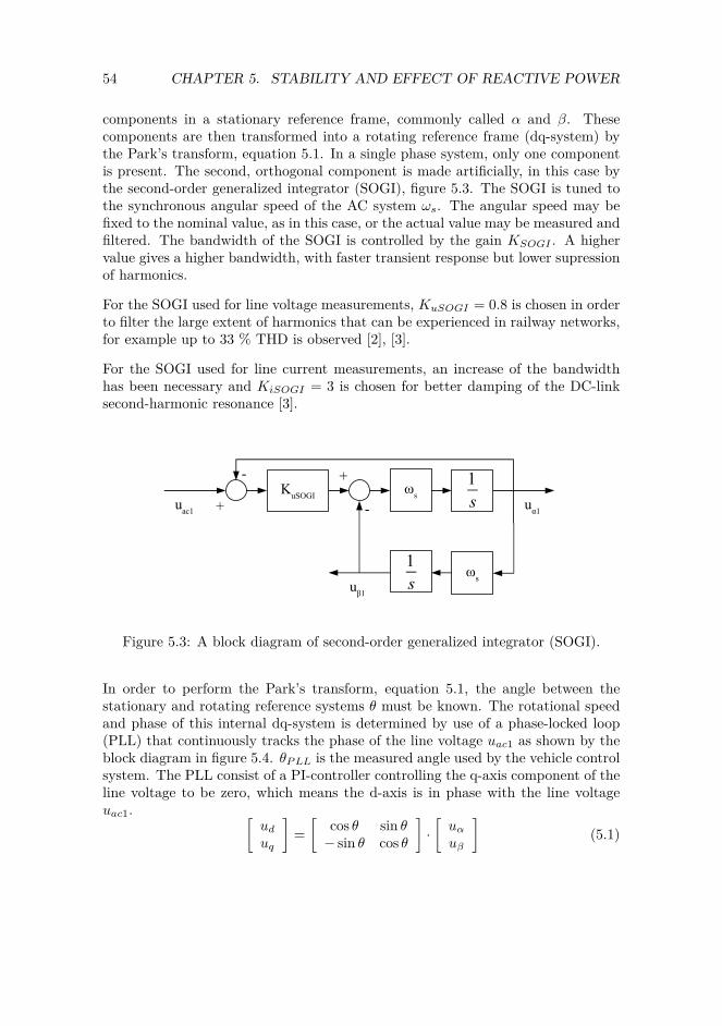
54 CHAPTER 5. STABILITY AND EFFECT OF REACTIVE POWER
components in a stationary reference frame, commonly called α and β. Thesecomponents are then transformed into a rotating reference frame (dq-system) bythe Park’s transform, equation 5.1. In a single phase system, only one componentis present. The second, orthogonal component is made artificially, in this case bythe second-order generalized integrator (SOGI), figure 5.3. The SOGI is tuned tothe synchronous angular speed of the AC system ωs. The angular speed may befixed to the nominal value, as in this case, or the actual value may be measured andfiltered. The bandwidth of the SOGI is controlled by the gain KSOGI . A highervalue gives a higher bandwidth, with faster transient response but lower supressionof harmonics.
For the SOGI used for line voltage measurements, KuSOGI = 0.8 is chosen in orderto filter the large extent of harmonics that can be experienced in railway networks,for example up to 33 % THD is observed [2], [3].
For the SOGI used for line current measurements, an increase of the bandwidthhas been necessary and KiSOGI = 3 is chosen for better damping of the DC-linksecond-harmonic resonance [3].
KuSOGI ωs
ωs
1s
1s
uac1 uα1
uβ1
-
+
+
-
Figure 5.3: A block diagram of second-order generalized integrator (SOGI).
In order to perform the Park’s transform, equation 5.1, the angle between thestationary and rotating reference systems θ must be known. The rotational speedand phase of this internal dq-system is determined by use of a phase-locked loop(PLL) that continuously tracks the phase of the line voltage uac1 as shown by theblock diagram in figure 5.4. θPLL is the measured angle used by the vehicle controlsystem. The PLL consist of a PI-controller controlling the q-axis component of theline voltage to be zero, which means the d-axis is in phase with the line voltageuac1. [
uduq
]=[
cos θ sin θ− sin θ cos θ
]·[uαuβ
](5.1)

5.1. SIMULATION MODEL 55
KpPLL
ud1
uq1
αβ
dq
uα1
uβ1
1TiPLL s
1s
+
+
+
+
ωff
θPLL
θPLL
x1
ωPLL
Figure 5.4: Phase locked loop (PLL).
5.1.4 Power Oscillation Damper
The structure of the power oscillation damper is shown in figure 5.5. The designof the POD is discussed by Danielsen in [3]. The first block represents the mea-surement of the voltage amplitude, which is used by several units in the controlsystem. When plotting the transfer function of the POD, the voltage measurementis modelled as a first order low pass with a time constant T1 = 0.02s. The secondblock is a high pass filter (wash-out filter), which will ensure that the steady stateoutput of the POD is zero. The third block is a lead-lag block which may be tunedto obtain the desired angle of the output. The gain of the controller may be chosen,as well as limits for the amplitude of the output signal.
T w sT w s1
T 2 s1T 3 s1
KPODud12 uq12ud1
uq1
+uPODlim
iqPOD (POD2)
-uPODlim
Figure 5.5: Power oscillation damper (POD).
5.1.5 Reactive Power Controller - QC
The reactive power controller is a cornerstone of this thesis and the main modifica-tion from the model proposed by Danielsen. In the model proposed by Danielsen,the q-axis current reference is constant equal to zero, giving unity power factorat the current collector in steady state. The reactive current controller, shown infigure 5.6 controls tanφref as a function of the voltage magnitude at the current
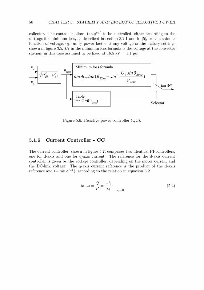
56 CHAPTER 5. STABILITY AND EFFECT OF REACTIVE POWER
collector. The controller allows tanφref to be controlled, either according to thesettings for minimum loss, as described in section 3.2.1 and in [5], or as a tabularfunction of voltage, eg. unity power factor at any voltage or the factory settingsshown in figure 3.5. U1 in the minimum loss formula is the voltage at the converterstation, in this case assumed to be fixed at 16.5 kV = 1.1 pu.
tan=tanZline−sin−1U 1 sinZline
uac1mud12 uq12
ud1
uq1
uac1m
Tabletan Φ=f(uac1m)
tan Φref
Minimum loss formula
Selector
Figure 5.6: Reactive power controller (QC).
5.1.6 Current Controller - CC
The current controller, shown in figure 5.7, comprises two identical PI-controllers,one for d-axis and one for q-axis current. The reference for the d-axis currentcontroller is given by the voltage controller, depending on the motor current andthe DC-link voltage. The q-axis current reference is the product of the d-axisreference and (− tanφref ), according to the relation in equation 5.2.
tanφ = Q
P= −iq
id uq=0(5.2)
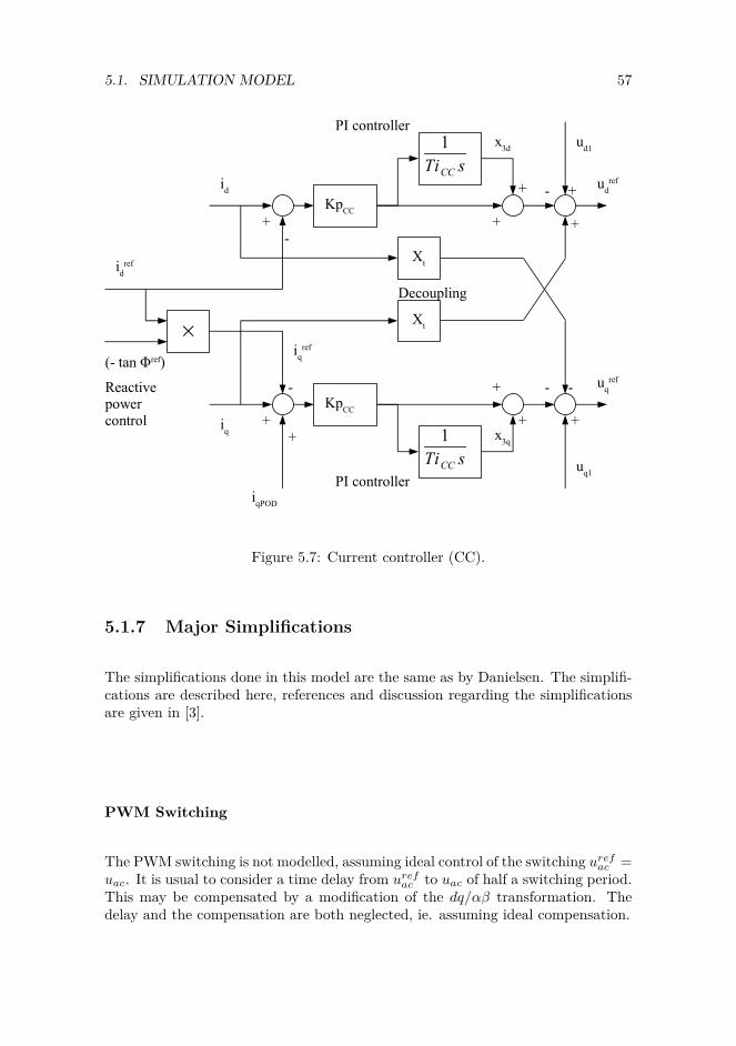
5.1. SIMULATION MODEL 57
KpCC
1TiCC s
+
+
x3d
+ -
udref
idref
×(- tan Φref)
KpCC
1TiCC s
+
+x3q
-
+ +
iqref
id
iq
iqPOD
uqref
Xt
Xt
Decoupling
PI controller
PI controller
Reactive power control
- -
+
- +
+
ud1
uq1
Figure 5.7: Current controller (CC).
5.1.7 Major Simplifications
The simplifications done in this model are the same as by Danielsen. The simplifi-cations are described here, references and discussion regarding the simplificationsare given in [3].
PWM Switching
The PWM switching is not modelled, assuming ideal control of the switching urefac =uac. It is usual to consider a time delay from urefac to uac of half a switching period.This may be compensated by a modification of the dq/αβ transformation. Thedelay and the compensation are both neglected, ie. assuming ideal compensation.
58 CHAPTER 5. STABILITY AND EFFECT OF REACTIVE POWER
Motor Side
Only a simple representation of the motor side is included in present model. In aquasi-stationary state the motor has to keep its power constant. If not, the torqueand further speed reference cannot be fulfilled. However, a motor side acting as aconstant power load for all frequencies, i.e., always increase the motor-side currentif the DC-link voltage drops, will reduce the stability of the DC-link.
In this work the motor side is described by equations 5.3 and 5.4. The motor isacting as a constant power load at frequencies below the low-pass filter bandwidth.MP is the voltage dependency at frequencies above the filter low-pass bandwidth.In this work MP = 2, equal to a constant impedance load.
pmotor(t) = prefmotor
(udc(t)
udc_filt(t)
)MP
(5.3)
udc_filt(s) = udc(s)TfCPL + 1 (5.4)
This motor power consumption is the only load in the vehicle model. Auxiliarypower consumption for heating, cooling, battery charging, control system powersupply etc. is not included neither from the DC-link nor from a separate trans-former winding.
Type of Controllers Used
The control system is implemented with analogue continuous controllers only.
Inverter and DC-link Structure
The structure of an advanced electric rail vehicle in real life may be more detailedthan shown in figure 2.3 and 2.4. There may be several DC-links per vehicle andseveral line- and motor-side inverters in parallel to each DC-link. In this model,all the vehicle’s DC-links are aggregated into a large one.
5.2 Impedance- and Admittance-based Represen-tation
5.2.1 Insufficiency of Eigenvalue Calculations
Eigenvalues is a common way of investigating a system’s small signal stability, andfunctions finding eigenvalues are commonly implemented in power system simula-

5.2. IMPEDANCE- AND ADMITTANCE-BASED REPRESENTATION 59
tion software. Eigenvalue analysis has however two important drawbacks.
Eigenvalues are calculated for a time invariant model, i.e. a rotating referenceframe. Rotating machines, transformers and lines are easily represented in a rotat-ing reference frame. Advanced control systems, and thereby the vehicle dynamicsmay be difficult to represent sufficiently in a rotating reference frame. Real-timesimulations may be of value if adequate power supply models can be provided,though they will still not provide explicit information of eigenvalues as they areperformed in a stationary reference frame and are hence time variant.
Eigenvalue calculations also require details of the vehicle including the controlsystem to be known. This is often not possible, as the manufacturers’ often considersuch details as industrial secrets.
Input admittance presented as frequency response characteristics is commonlyavailable for describing the vehicle’s behaviour at frequencies above the fundamen-tal, used to determine electric resonance stability. Similar data could be providedby the manufacturers for the low frequency domain; however, this is not known bythe author to be praxis.
5.2.2 Impedance and Admittance
The Thevenin equivalent is well known within electrical engineering, where a net-work of voltage sources, current sources and impedances can, seen from one pointof the network, be replaced by a voltage source and an impedance. The voltagesource describes the voltage at this point of the network before a change is done,the impedance describes the change of voltage when a current in injected into thispoint. The Thevenin equivalent is only valid for a network consisting of only con-stant voltage and current sources, and constant impedances, linear components.A system with non-linear components may also be represented this way, but thisrepresentation will only be valid at one operating point.
An AC system may be described by as vectors, e.g. in d- and q-components. Inan AC system with rotary machines, power electronics and advanced controllers,the response to d-axis current may be fundamentally different from the responseto q-axis current. An example could be the output voltage of a rotary converterwith a voltage regulator controlling the voltage magnitude to be kept constant.Assuming the d-axis reference is the voltage, a d-axis current (real power load) willcause the voltage angle to lag compared to the no-load situation. A q-axis current(reactive power) will on the other hand give a very small response, as it will notcause any significant change of voltage phase, and the voltage magnitude is (atleast stationary) kept constant by the voltage regulator.
The dynamic properties of the source is represented as impedance, change of voltageper change of current, equation 5.5. Similarly, the load (in this case the vehicle)is represented as an admittance, change of current per change of voltage, equation

60 CHAPTER 5. STABILITY AND EFFECT OF REACTIVE POWER
5.6. To reflect a dynamic system, the impedance and admittance will normally befrequency dependent.
Zsource = ∆U∆I (5.5)
Yload = ∆Iload∆U (5.6)
The source impedance and load admittance can be found by observing the responsesfrom the load and the source to a disturbance current injected, ∆Is. The loadadmittance does not describe the inner workings of the load’s control system, onlythe current output for a given voltage input. The impedance and admittanceare depending on the operating point, and must thereby be given for a specifiedoperating point.
~ ↓
I= I0 + ΔI
U=U0+ ΔUZsource
ZloadUth I0
Source Load
ΔI
Interface
↓ΔIS
ΔIload
Figure 5.8: Equivalent circuit.
The system can be shown as a control system with feedback, being exposed to adisturbance, as shown in figure 5.9. When the disturbance ∆Is is known, as wellas the system’s response ∆I and ∆U ; Yload and Zsource can be found by solvingequations 5.7. This solution is valid for the frequency of the injected disturbance.A frequency sweep of ∆Is may be performed to obtain Yload and Zsource for a rangeof frequencies.

5.2. IMPEDANCE- AND ADMITTANCE-BASED REPRESENTATION 61
Yload
Zsource
ΔIload
ΔIs
ΔI
+
-
ΔU(ΔUs) +
+
Figure 5.9: Impedance model shown as control system.
∆Iload = ∆I −∆Is = Yload ·∆U−∆U = Zsource ·∆I
(5.7)
An AC system may be transformed by the Park’s transform into a synchronouslyrotating reference frame, where AC quantities are transformed into two orthogonalDC components, commonly known as a dq-system. The transformed system isshown as a multiple input - multiple output (MIMO) as shown in figure 5.8.

62 CHAPTER 5. STABILITY AND EFFECT OF REACTIVE POWER
Ydd
Yqd
ΔIsd
Ydq
Yqq
Zdd
Zqd
Zdq
Zqq
ΔIq
ΔUd
ΔUq
+
-
+
+
+
-
+
+
+
+
+
+
Yload
Zsource
ΔId
ΔIload d +
+
+
+
ΔIsq
ΔIload q
Figure 5.10: Impedance model shown as control system for d- and q-components.
In the MIMO system, the input and output signals may be represented by vectors,and the source impedance and the load admittance as matrices, according to therelations in equation 5.8. The matrices [Yload] and [Zsource] can be found by twomeasurements or simulations, by injecting a pure d-axis, and pure q-axis distur-bance current, and solving equation 5.8. The solution of the equations are given in[10].
• One sweep with pure d-axis disturbance current; ∆Isd1 6= 0 and ∆Isq1 = 0
• One sweep with pure q-axis disturbance current; ∆Isd2 = 0 and ∆Isq2 6= 0
When the d-axis is aligned with the voltage at the interface, the Zdd and Zqd will

5.2. IMPEDANCE- AND ADMITTANCE-BASED REPRESENTATION 63
represent the power supply’s response to real power (d-axis current), while Zdq andZqq will represent the power supply’s response to reactive power.
A change of d-axis voltage ∆Ud represents a change of voltage magnitude, whilea change q-axis voltage ∆Uq represents a change of voltage angle. Ydd and Yqdrepresent the load’s response to a change of voltage magnitude, while Ydq and Yqqrepresent the load’s response to a change of voltage angle.
[∆Iload d∆Iload q
]=[
∆Id −∆Isd∆Iq −∆Isq
]=[Ydd YdqYqd Yqq
]·[
∆Ud∆Uq
]−[
∆Ud∆Uq
]=[Zdd ZdqZqd Zqq
]·[
∆Id∆Iq
] (5.8)
5.2.3 Analytical Considerations
To improve understanding of what the load admittance represents, as well as check-ing the simulation output, the expressions for the steady state admittance of aregulated constant power load are developed.
U and I indicate the voltage and current magnitude at the interface between sourceand load, while U and I indicate phasor quantities.
U1 indicates the voltage magnitude at the terminals of the rotary converter station,which is assumed to be fixed at 16.5 kV = 1.1 pu in the minimum loss formula,equation 3.1. θZ line is the impedance angle of the overhead line. With the typicalvalue Zline = (0.19 + j0.21)Ω/km, θZ line = 47.86.
P and Q are the real and reactive power measured at the interface. S is theapparent power magnitude, while the phasor S = P + jQ.
δ is the voltage angle at the interface. When transforming into d- and q-components,the d-axis reference is the interface voltage, and δ ≡ 0. φ is the angle between cur-rent and voltage at the interface, where current lagging the voltage gives a positiveangle. With δ = 0, φ = − arg I.
For load with constant real and reactive power, the sensitivity to a change of voltagemagnitude is given by equation 5.9.

64 CHAPTER 5. STABILITY AND EFFECT OF REACTIVE POWER
S = U · I∗
I = P − jQU
= S∗
U
dI
dU= −P − jQ
U2 = − S∗
U2
Y = dI
dU= − S
U2 = − P
U2 · cosφ= − Q
U2 · sinφ
(5.9)
For a load where P and Q are depending on voltage magnitude, the current magni-tude I and the load angle φ will be voltage dependant. The sensitivities to changeof voltage angle and magnitude are given in equation 5.10. For a load where realand reactive power has the same voltage sensitivity, e.g. a constant impedance orconstant power load, φ will be independent of voltage, i.e. dφ
dU = 0. A limitation ofcurrent or power as a function of voltage, e.g. the current limitation according toEN50388:2005 as described in section 3.1.2, will affect dI
dU .
I = I · ej(δ−φ)
U = U · ejδ
dI
dU= dI
dU· ej(δ−φ) − I · ej(δ−φ) · j dφ
dU
dI
dδ= jI · ej(δ−φ) = jI
(5.10)
With φ as a function of voltage magnitude, dφdU 6= 0. The voltage sensitivity of theminimum loss characteristic is shown in equation 5.11.
φ(U) = θZ line − sin−1 U1 · sin θZ line
U= θZ line − sin−1 x
dφ
dU= − 1√
1− x2· dxdU
= 1√1− (U1·sin θZ line
U )2· U1 · sin θZ line
U2
= 1√1− (U1·Xline
U·Zline)2· U1 ·Xline
U2 · Zline
(5.11)
The de-composition into d- and q-components is for a general characteristic (bothP = f(U) and Q = g(U)) is shown in equation 5.12.

5.2. IMPEDANCE- AND ADMITTANCE-BASED REPRESENTATION 65
dUd = dU
Ydd = dIddUd
= dIddU
= RedI
dU= dI
dU· cosφ− I dφ
dU· sinφ
Yqd = dIddUd
= dIqdU
= ImdI
dU= − dI
dU· sinφ− I dφ
dU· cosφ
dUq = dδ2 · U
Ydq = dIddUq
= dIddδ2 · U
= Re(jI)U
= Re(jI · e−jφ)U
= −I sin(−φ)U
= I sinφU
Yqq = dIqdUq
= dIqdδ2 · U
= Im(jI)U
= Im(jI · e−jφ)U
= I cos(−φ)U
= I cosφU
(5.12)
To perform a given mechanical work, the real power is to be kept constant whendisregarding losses. If reactive power control is implemented under such conditions,the real power P will be constant and dP
dU = 0. The sensitivity of the reactivepower Q to voltage is shown in equation 5.13, an further used to find the current’ssensitivity to voltage in equation 5.14.
Q = P · tanφdQ
dU= P · d(tanφ)
dU= P · 1
cos2 φ· dφdU
(5.13)
I =√P 2 +Q2
U= U−1 ·
√P 2 +Q2
dI
dU= U−1 · 1
2√P 2 +Q2
· 2Q · dQdU
+ (−U−2) ·√P 2 +Q2
= 1U ·√P 2 +Q2
·Q · P · 1cos2 φ
· dφdU−√P 2 +Q2
U2
(5.14)
Current, cosφ and sinφ can be replaced by powers and voltage, giving the finaladmittance values shown in equation 5.15. For the minimum loss settings, withoutlimitation of the real power, dφdU is shown in equation 5.11 and dI
dU in equation 5.14.

66 CHAPTER 5. STABILITY AND EFFECT OF REACTIVE POWER
Ydd = dIddUd
= dI
dU· cosφ− I dφ
dU· sinφ = dI
dU· cosφ− dφ
dU· QU
Yqd = dIqdUd
= − dIdU· sinφ− I dφ
dU· cosφ = − dI
dU· sinφ− dφ
dU· PU
Ydq = dIddUq
= −I sin(−φ)U
= I sinφU
= Q
U2
Yqq = dIqdUq
= I cos(−φ)U
= P
U2
(5.15)
If the source impedance is a line only, the impedance matrice for steady state isshown in equation 5.16. The source impedance of a rotary converter with automaticvoltage regulator is not calculated analytically here.[
Zdd ZdqZqd Zqq
]=[
R −ωs · Lωs · L R
](5.16)
5.2.4 Stability Criterion
In [11], the control loops shown in figure 5.10 are considered as a MIMO systemand the generalized Nyquist stability criterion is applied.
Theorem Generalised Nyquist theorem for a MIMO system1: Let Poldenote the number of open-loop unstable poles in L(s). The closed-loop systemwith loop transfer function L(s) and negative feedback is stable if and only if theNyquist plot of det([I]+L(s)) makes Pol anti-clockwise encirclements of the origin,and does not pass through the origin.
From this it may be derived ([12]) that the Nyquist contour N(s) should make noencirclements of the origin if [Zsource] · [Yload] is open-loop stable, and should makePol anti-clockwise encirclements if [Zsource] · [Yload] is unstable. N(s) is given inequation 5.17, with the angular speed of oscillation ωosc.
N(s) = det([I] + [Zsource] · [Yload])|s=jωosc (5.17)
Writing out the elements of the matrices, this criterion may be interpreted as theNyquist Contour -1 (N-1) in equation 5.18 should not clockwise encircle (-1+j0)as the commonly known Nyquist stability criterion for single-input-single-output
1Theorem 4.9 in [12]

5.3. EFFECT OF A PASSIVE CONTROL OF REACTIVE POWER 67
(SISO) systems.
N(s)− 1 = YddYqqZddZqq + YdqYqdZdqZqd
− YdqYqdZddZqq − YddYqqZdqZqd+ YddZdd + YqqZqq + YdqZqdYqdZdq
(5.18)
If this interpretation is accepted, the amplitude and phase plot of (N-1) can bepresented as well for this MIMO system such as in a SISO system [10].
5.3 Effect of a Passive Control of Reactive Power
The following cases are simulated and compared. The control schemes are describedfor steady state in section 3.2.1 and in [5]:
1. Unity power factor. This is the reference case, also used as reference case byDanielsen.
2. "Minimum loss", static φ. In this case, the operating point is given by the"minimum loss" characteristics. The "minimum loss" characteristics give avoltage dependent load angle φ, but this voltage dependency is disregardedin dynamic analyses, keeping φ constant at the value from the load flowcalculation. This case is chosen to distinguish the effect of changed operatingpoint from the effect of reactive power control. Such a characteristic could beimplemented by having a slow response from the reactive power controller,or by having a constant load angle over a voltage range, such as "factorysettings" below 13 kV, shown in figure 3.5.
3. "Minimum loss", dynamic φ. In this case, the operating point is given by the"minimum loss" characteristics. The reactive power controller controls theq-axis current reference iqref without intended delay (although some delay iscaused by the voltage measurement and the current controller).
The vehicle is operating at half the rated power, 3.67 MW at the DC link, giv-ing approximately 3.8 MW at the current collector. No power oscillation damper(POD) is used. The simulations are run in TRANSTA, using enhanced RMS asdescribed in [3].
The control schemes for reactive power in steady state described in section 3.2.1 allcontrol q-axis current reference by multiplying the d-axis current reference by theoutput from the reactive power controller. In no-load, the d-axis current referenceis zero, so that the reactive power controller has no effect in no-load. Therefore,these control schemes are not compared in no-load.

68 CHAPTER 5. STABILITY AND EFFECT OF REACTIVE POWER
5.3.1 Operating Points and Steady State Considerations
Operating Points
The operating points for the simulations are shown in table 5.1. Note that thereal power is slightly lower for the "minimum loss" cases, due to lower transformerlosses.
Table 5.1: Operating pointsUnit Simulation case
Unity powerfactor
"Minimumloss", static φ
"Minimum loss",dynamic φ
Uloco kV 12.61 13.71 13.71Ploco MW 3.811 3.798 3.798Qloco MVAr 0.000 -1.039 -1.039Iloco kA 0.3023 0.2871 0.2871φ 0 -15.3 -15.3φ rad 0 -0.267 -0.267dφ/dUloco
rad/kV 0 0 0.1441dI/dUloco
kA/kV -0.0240 -0.0209 -0.0323
Steady State Admittance Matrices
The steady state admittance matrices are calculated according to equation 5.15.There is a small inaccuracy in the values calculated here, as the formula is developedfor a constant real power. In this case, the real power is constant 3.67 MW at theDC-link, but will vary slightly at the current collector as the current and therebythe transformer loss is depending on operating voltage, i.e. the vehicle is not aperfect constant power load at the current collector.
Unity power factor:
Y =[−0.0240 0
0 0.0240
][A/V ]
"Minimum loss", static φ:
Y =[−0.0202 −0.0055−0.0055 0.0202
][A/V ]
"Minimum loss", dynamic φ:
Y =[−0.0202 −0.0055−0.0484 0.0202
][A/V ]
All the admittances have negative Ydd, i.e. increased voltage magnitude givesreduced d-axis current, which is as expected for a load with constant real power.

5.3. EFFECT OF A PASSIVE CONTROL OF REACTIVE POWER 69
Effect of Rotary Converter Voltage Deviation
A constant power load is exactly that, constant power. In this case, the motorside inverter draws a constant power of 3.67 MW from the DC-link. The line sideconverter in the vehicle is modelled as lossless, ie. the the vehicle is a constant powerload at the low voltage side of the vehicle main transformer. Constant power causesreduced voltage to be compensated by increased current. If the constant powerload is supplied by a transmission which is not lossless, reduced voltage will causeincreased power. This is most likely an effect reducing voltage stability; reducedvoltage increases the power consumption, which will cause a further decrease ofvoltage.
This effect is shown in table 5.2. Load flow calculation is performed in normaloperation, the voltage at the converter station Ucon = 16.5 kV, as well as ± 1 %(± 165 V). Voltage decrease gives a slight increase at the power at the vehicle’scurrent collector Ploco, and a larger increase in the line loss Pline loss.
With unity power factor at the vehicle, a voltage deviation at the converter stationof 165 V gives a deviation of the vehicle voltage Uloco of 266-275 V. For "minimumloss", static φ, the voltage deviates 231-235 V, while "minimum loss", dynamic φgives a voltage deviation at the vehicle of 150-152 V.
Table 5.2: Stationary response to voltage deviation at the converter station. Volt-age in [kV], real power in [MW] and reactive power in [MVAr].Ucon Uloco ∆Uloco Ploco Qloco tanφloco Pline lossUnity power factor16.665 (+1 %) 12.874 0.266 3.805 0 0 0.995916.500 (ref) 12.608 - 3.811 0 0 1.041716.335 (-1 %) 12.333 -0.275 3.818 0 0 1.0927Minimum loss, static φ16.665 (+1 %) 13.943 0.231 3.793 -1.037 -0.273 0.906716.500 (ref) 13.713 - 3.798 -1.039 -0.273 0.939716.335 (-1 %) 13.478 -0.235 3.802 -1.040 -0.273 0.9752Minimum loss, dynamic φ16.665 (+1 %) 13.865 0.152 3.793 -0.951 -0.251 0.906816.500 (ref) 13.713 - 3.798 -1.039 -0.273 0.939716.335 (-1 %) 13.563 -0.150 3.802 -1.132 -0.298 0.9754
5.3.2 Eigenvalue Considerations
For the three cases given, the system’s eigenvalues are calculated. Out of a totalof 41 eigenvalues (zero-values excluded), the ones having a frequency lower thanthe fundamental frequency (Im(λ) < fs) and a real part larger than -100 (Re(λ) >
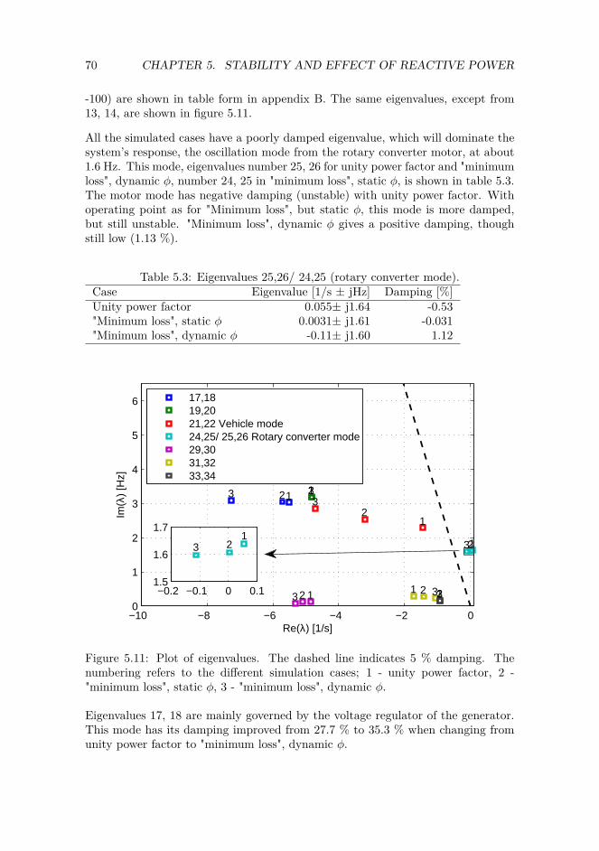
70 CHAPTER 5. STABILITY AND EFFECT OF REACTIVE POWER
-100) are shown in table form in appendix B. The same eigenvalues, except from13, 14, are shown in figure 5.11.
All the simulated cases have a poorly damped eigenvalue, which will dominate thesystem’s response, the oscillation mode from the rotary converter motor, at about1.6 Hz. This mode, eigenvalues number 25, 26 for unity power factor and "minimumloss", dynamic φ, number 24, 25 in "minimum loss", static φ, is shown in table 5.3.The motor mode has negative damping (unstable) with unity power factor. Withoperating point as for "Minimum loss", but static φ, this mode is more damped,but still unstable. "Minimum loss", dynamic φ gives a positive damping, thoughstill low (1.13 %).
Table 5.3: Eigenvalues 25,26/ 24,25 (rotary converter mode).Case Eigenvalue [1/s ± jHz] Damping [%]Unity power factor 0.055± j1.64 -0.53"Minimum loss", static φ 0.0031± j1.61 -0.031"Minimum loss", dynamic φ -0.11± j1.60 1.12
−10 −8 −6 −4 −2 00
1
2
3
4
5
6
Re(λ) [1/s]
Im(λ
) [H
z]
1 1
1
1
1 1 1
2 2
2
2
2 2 2
3 33
3
3 33
17,1819,2021,22 Vehicle mode24,25/ 25,26 Rotary converter mode29,3031,3233,34
−0.2 −0.1 0 0.11.5
1.6
1.71
23
Figure 5.11: Plot of eigenvalues. The dashed line indicates 5 % damping. Thenumbering refers to the different simulation cases; 1 - unity power factor, 2 -"minimum loss", static φ, 3 - "minimum loss", dynamic φ.
Eigenvalues 17, 18 are mainly governed by the voltage regulator of the generator.This mode has its damping improved from 27.7 % to 35.3 % when changing fromunity power factor to "minimum loss", dynamic φ.

5.3. EFFECT OF A PASSIVE CONTROL OF REACTIVE POWER 71
The vehicle mode 21, 22, is clearly influenced by the settings for reactive power.When changing from unity power factor to "minimum loss", dynamic φ, the eigen-value is changed from -1.42 [1/s] ± j2.28 [Hz] to -3.29 [1/s] ± j2.85 [Hz], andincrease of damping from 9.9 % to 18.1 %. The eigenvalues 31, 32 are dominatedby the generator. These are also affected by the settings for reactive power, beingchanged from -1.42 [1/s] ± j0.35 [Hz] to -0.94 [1/s] ± j0.24 [Hz], but they will havelittle effect, as their damping in all cases is about 50 %.
Eigenvalues 29, 30 are governed by the vehicle. This mode is somewhat influencedby settings for reactive power, but has in all cases a damping about 99 %.
Eigenvalues 19, 20 and 33, 34 are mainly governed by the voltage regulator, exciterand field winding of the 3-phase motor. Reactive power settings on the single phaseside has no significant influence on these modes.
5.3.3 Impedance and Admittance Considerations
Frequncy sweeps are performed to find [Zsource] and [Yload] for frequencies from0.01 to 16 Hz. The impedance and admittance values are shown graphically inattachment C.
The Nyquist contour (N-1) is shown in figure 5.12. The curve for unity powerfactor encircles the point (-1+j0), which indicates an unstable system. The curvefor "minimum loss", static φ passes very close to the point (-1+j0), which indicatesan unstable or marginally stable system. The curve for "minimum loss", dynamicφ does not encircle (-1+j0), which indicates a stable system. Three points of thiscurve is located far from the others, forming "spikes" out from the rest of the curve.These points are assumed to be caused by an inaccuracy in the simulation, andcan probably be neglected when considering the result.

72 CHAPTER 5. STABILITY AND EFFECT OF REACTIVE POWER
−2.5 −2 −1.5 −1 −0.5 0 0.5 1 1.5 2−1.5
−1
−0.5
0
0.5
1
1.5
2
2.5
3Nyquist plot
Re(N−1)
Im(N
−1)
−2 −1.5 −1 −0.5 0−1
−0.5
0
0.5
1Nyquist zoom
Re(N−1)
Im(N
−1)
Unity power factor"Minimum loss", static φ"Minimum loss", dynamic φ
Figure 5.12: Contour of (N-1) for the three simulation cases.
5.3.4 Time Simulations
A 100 kW load is connected at the rotary converter 16.5 kV bus at t=-0.1 s, anddisconnected at t=0 s. Rotary converter speed ωgen, voltage Uloco and powers(Ploco and Qloco) at the vehicle are shown in figure 5.13 and 5.14. Note that thereare two different axes for voltage and reactive power due to different operatingpoints.
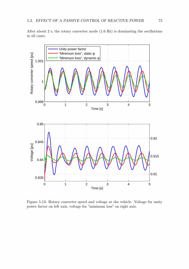
5.3. EFFECT OF A PASSIVE CONTROL OF REACTIVE POWER 73
After about 2 s, the rotary converter mode (1.6 Hz) is dominating the oscillationsin all cases.
0 1 2 3 4 50.999
1
1.001
Time [s]
Rot
ary
conv
erte
r sp
eed
[pu]
Unity power factor"Minimum loss", static φ"Minimum loss", dynamic φ
0 1 2 3 4 5
0.835
0.84
0.845
0.85
Time [s]
Vol
tage
[pu]
0.91
0.915
0.92
Figure 5.13: Rotary converter speed and voltage at the vehicle. Voltage for unitypower factor on left axis, voltage for "minimum loss" on right axis.

74 CHAPTER 5. STABILITY AND EFFECT OF REACTIVE POWER
0 1 2 3 4 50.59
0.592
0.594
0.596
0.598
0.6
Time [s]
Rea
l pow
er [p
u]
Unity power factor"Minimum loss", static φ"Minimum loss", dynamic φ
0 1 2 3 4 5−0.002
−0.001
0
0.001
0.002
Time [s]
Rea
ctiv
e po
wer
[pu]
−0.164
−0.163
−0.162
−0.161
−0.16
Figure 5.14: Real and reactive power at the vehicle. Reactive power for unitypower factor on left axis, reactive power for "minimum loss" on right axis.
The oscillations from figure 5.13 and 5.14 are shown as phasors in figure 5.15 andtable 5.4, together with voltage angle at the vehicle δloco, the real power of rotaryconverter generator Pgen, the electromagnetic torque Tgen and the voltage of theconverter station’s 15 kV busbar Ucon. The electromagnetic torque is found as thereal power of the generator divided by the speed. The phasors are found by fastfourier transform over one fundamental period at t ≈ 2.5 s. The phasors are shownin pu relative to the rotary converter speed, ie. what is the system’s response to a

5.3. EFFECT OF A PASSIVE CONTROL OF REACTIVE POWER 75
given mechanical oscillation.
Damping of mechanical oscillations would be load torque (electromagnetic torqueof generator = load torque of mechanical system) oscillating in phase with thespeed, increased speed giving increased load torque. In all three cases, the vehiclecontributes to destabilizing the the system, as the torque oscillations have a phase> 90 from the speed oscillations. In table 5.4, this is shown as negative real part.
The voltage oscillations for "minimum loss", dynamic φ are clearly smaller thanfor "minimum loss", static φ and unity power factor, which indicates that thereactive power from the vehicle helps stabilizing the system voltage. "Minimumloss", dynamic φ also gives smaller oscillations of the voltage angle at the vehicle.A similar effect is shown in table 5.2, where a 165 V change of the voltage at therotary converter station gives a change of the vehicle voltage of 266-275 V withunity power factor, but only 150-152 V for "minimum loss", dynamic φ.
Smaller oscillations of voltage magnitude and angle at the vehicle give smalleroscillations in the vehicle real power, reducing the vehicle’s destabilizing impact onthe system.
Unity power factor "Minimum loss", static φ
"Minimum loss", dynamic φ
ω
gen
Ucon
Pgen
Tgen
Uloco
δloco
Ploco
Qloco
Figure 5.15: Oscillations after disturbance shown as phasors. The speed phasor isset to 1, other phasors scaled accordingly. Positive direction for real and reactivepower is from the rotary converter to the vehicle.

76 CHAPTER 5. STABILITY AND EFFECT OF REACTIVE POWER
Table 5.4: Oscillations after disturbance shown as phasors. The speed phasor isset to 1, other phasors scaled accordingly.
Unity power factor "Minimum loss",static φ
"Minimum loss",dynamic φ
ωgen 1 1 1Ucon 2.24+j1.15 2.08+j0.54 1.27+j0.21Pgen -2.63-j2.26 -2.45-j0.62 -1.43-j0.04Tgen -3.40-j2.26 -3.20-j0.62 -2.18-j0.04Uloco 3.60+j2.47 3.19+j0.95 1.23+j0.27δloco 0.57-j1.67 0.55-j1.93 0.29-j1.34Ploco -0.76-j0.69 -0.87-j0.12 -0.48+j0.07Qloco 0.46+j0.09 0.44+j0.11 2.06+j0.11
5.4 Effect of Active Control of Reactive Power -POD
The main purpose of this section is not to find the optimal settings for the PODs,but to investigate the potential of using reactive power for damping oscillations.The dominating oscillation in the system in traction is the rotary converter modeat approximately 1.6 Hz. In no-load, the system will become unstable at long linelengths with an oscillation caused by the vehicle at 4-5 Hz.
The structure of the power oscillation damper (POD) is shown in section 5.1.4.Two different PODs are tested in traction and no-load.
5.4.1 Design of POD
All PODs use the voltage magnitude as input, and send the output signal to thesummation point of the q-axis current controller. As negative q-axis current corre-sponds to positive reactive power, −iq POD is shown in graphs and phasor diagrams.
POD2a
POD2a is designed by Danielsen, called POD2 in [3]. POD2 aims to reduce theline voltage oscillations at the rotary converter eigenfrequency by means of reac-tive power modulation. The pass-band filter created by the measurement blockand the wash-out block are chosen to be symmetrical around the rotary convertereigenfrequency. This results in a zero phase of the filter at 1.6 Hz, and no extralead and lag block is used.

5.4. EFFECT OF ACTIVE CONTROL OF REACTIVE POWER - POD 77
POD2b
POD2b was tuned to damp the vehicle mode which may cause instability in no-load.
A POD with no change of phase except from voltage measurement and KPOD = 0was implemented in the model and simulated in no-load, with KPOD = 0. Thesensitivity of the vehicle mode (0.111 1/s ± j4.324 Hz) to KPOD was found to2.560 1/s/pu ± j1.617 Hz/pu, giving an angle of -75 from moving the eigenvaluestraight to the left. During parameter scanning POD2a in no-load (figure 5.21),scanning of Tw indicated a minimum of Re(λ) with Tw = 0.03s. The lead-lag blockwas tuned so that the wash-out and the lead-lag totally increased the phase by75 at 4.32 Hz. The gain was first set to 1. At this setting, the vehicle modedecayed too fast to perform Fourier analysis over a complete cycle, and the gainwas reduced to 0.5.
The POD parameters are shown in figure 5.5, and resulting bode plots are shownin figure 5.16.
10−2
10−1
100
101
102
103
0
0.25
0.5
0.75
1
Frequency [Hz]
Mag
nitu
de [a
bs]
H
POD2a(s)
HPOD2b
(s)
10−2
10−1
100
101
102
103
−90
−45
0
45
90
Frequency [Hz]
Pha
se [° ]
Figure 5.16: Bodeplots of POD transfer functions.

78 CHAPTER 5. STABILITY AND EFFECT OF REACTIVE POWER
Table 5.5: POD parameters.Parameter Unit POD2a POD2bT1 [s] 0.02 0.02Tw [s] 0.47 0.03T2 [s] 0 0.05T3(= TPOD) [s] 0 0.02KPOD [pu] 1 0.5uPODlim [pu] 0.01 0.01
5.4.2 Traction - Damping of Rotary Converter mode
The vehicle is investigated in traction, at the operating point "minimum loss",dynamic φ in table 5.1. The settings used for reactive power is "minimum loss",dynamic φ, without POD, as well as with POD2a and POD2b. Unity power factoris already investigated by Danielsen, "minimum loss", static φ is primarily madeas a reference case to distinguish the effect of dynamic control of reactive powerfrom the effect of operating point. "Minimum loss", dynamic φ also yielded thebest damping of the rotary converter mode.
−10 −8 −6 −4 −2 00
1
2
3
4
5
1 11
1
2 22
2
333
3
Re(λ) [1/s]
Im(λ
) [H
z]
Vehicle modeGenerator exciter modeMotor exciter modeRotary converter mode
−0.1 −0.05 01.59
1.595
1.6
12
3
Figure 5.17: Plot of eigenvalues without POD (1) and with POD2a (2) and POD2b(3). The dashed line indicates 5 % damping.
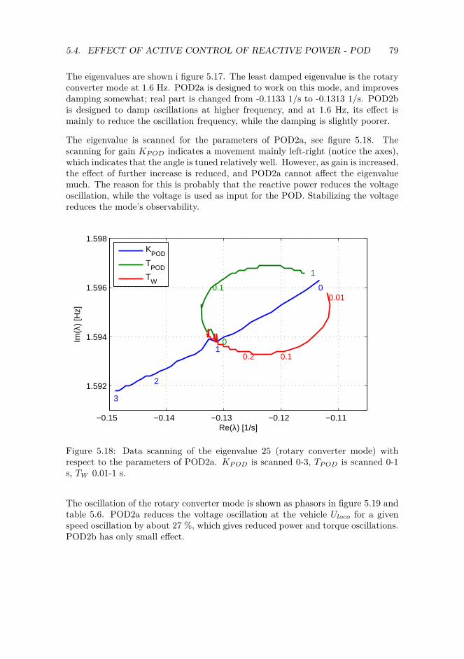
5.4. EFFECT OF ACTIVE CONTROL OF REACTIVE POWER - POD 79
The eigenvalues are shown i figure 5.17. The least damped eigenvalue is the rotaryconverter mode at 1.6 Hz. POD2a is designed to work on this mode, and improvesdamping somewhat; real part is changed from -0.1133 1/s to -0.1313 1/s. POD2bis designed to damp oscillations at higher frequency, and at 1.6 Hz, its effect ismainly to reduce the oscillation frequency, while the damping is slightly poorer.
The eigenvalue is scanned for the parameters of POD2a, see figure 5.18. Thescanning for gain KPOD indicates a movement mainly left-right (notice the axes),which indicates that the angle is tuned relatively well. However, as gain is increased,the effect of further increase is reduced, and POD2a cannot affect the eigenvaluemuch. The reason for this is probably that the reactive power reduces the voltageoscillation, while the voltage is used as input for the POD. Stabilizing the voltagereduces the mode’s observability.
−0.15 −0.14 −0.13 −0.12 −0.11
1.592
1.594
1.596
1.598
Re(λ) [1/s]
Im(λ
) [H
z]
0
1
2
3
0
0.1
1
0.01
0.1 0.2
KPOD
TPOD
TW
Figure 5.18: Data scanning of the eigenvalue 25 (rotary converter mode) withrespect to the parameters of POD2a. KPOD is scanned 0-3, TPOD is scanned 0-1s, TW 0.01-1 s.
The oscillation of the rotary converter mode is shown as phasors in figure 5.19 andtable 5.6. POD2a reduces the voltage oscillation at the vehicle Uloco for a givenspeed oscillation by about 27 %, which gives reduced power and torque oscillations.POD2b has only small effect.
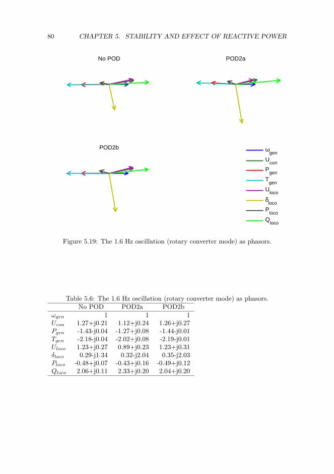
80 CHAPTER 5. STABILITY AND EFFECT OF REACTIVE POWER
No POD POD2a
POD2b
ω
gen
Ucon
Pgen
Tgen
Uloco
δloco
Ploco
Qloco
Figure 5.19: The 1.6 Hz oscillation (rotary converter mode) as phasors.
Table 5.6: The 1.6 Hz oscillation (rotary converter mode) as phasors.No POD POD2a POD2b
ωgen 1 1 1Ucon 1.27+j0.21 1.12+j0.24 1.26+j0.27Pgen -1.43-j0.04 -1.27+j0.08 -1.44-j0.01Tgen -2.18-j0.04 -2.02+j0.08 -2.19-j0.01Uloco 1.23+j0.27 0.89+j0.23 1.23+j0.31δloco 0.29-j1.34 0.32-j2.04 0.35-j2.03Ploco -0.48+j0.07 -0.43+j0.16 -0.49+j0.12Qloco 2.06+j0.11 2.33+j0.20 2.04+j0.20
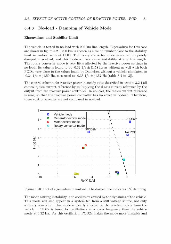
5.4. EFFECT OF ACTIVE CONTROL OF REACTIVE POWER - POD 81
5.4.3 No-load - Damping of Vehicle Mode
Eigenvalues and Stability Limit
The vehicle is tested in no-load with 200 km line length. Eigenvalues for this caseare shown in figure 5.20. 200 km is chosen as a round number close to the stabilitylimit in no-load without POD. The rotary converter mode is stable but poorlydamped in no-load, and this mode will not cause instability at any line length.The rotary converter mode is very little affected by the reactive power settings inno-load. Its value is found to be -0.32 1/s ± j1.58 Hz as without as well with bothPODs, very close to the values found by Danielsen without a vehicle; simulated to-0.34 1/s ± j1.59 Hz, measured to -0.33 1/s ± j1.57 Hz (table 3-2 in [3]).
The control schemes for reactive power in steady state described in section 3.2.1 allcontrol q-axis current reference by multiplying the d-axis current reference by theoutput from the reactive power controller. In no-load, the d-axis current referenceis zero, so that the reactive power controller has no effect in no-load. Therefore,these control schemes are not compared in no-load.
−10 −8 −6 −4 −2 00
1
2
3
4
5
6
7
Re(λ) [1/s]
Im(λ
) [H
z]
No POD
POD2a
POD2b
Vehicle modeGenerator exciter modeMotor exciter modeRotary converter mode
Figure 5.20: Plot of eigenvalues in no-load. The dashed line indicates 5 % damping.
The mode causing instability is an oscillation caused by the dynamics of the vehicle.This mode will also appear in a system fed from a stiff voltage source, not onlya rotary converter. This mode is clearly affected by the reactive power from thevehicle. POD2a is tuned for oscillations at a lower frequency than the vehiclemode at 4.32 Hz. For this oscillation, POD2a makes the mode more unstable and

82 CHAPTER 5. STABILITY AND EFFECT OF REACTIVE POWER
increases its frequency.
POD2b is tuned for damping the vehicle mode, and damps the mode well withonly a minor change of frequency. Similar effects can be seen on the stabilitylimits shown in table 5.7. POD2a increases frequency and decreases stability limit.POD2b has less effect on frequency, while the stability limit is nearly doubled, seetable 5.7.
Table 5.7: The stability limit with and without POD.Model Stability limit [km] Oscillation frequency [Hz]No POD 197 4.35POD2a 193 5.84POD2b 341 4.06
Parameter Scanning
Parameter scanning of KPOD at POD2a shows clearly how it increases frequencywith little effect on the damping, figure 5.21. Scanning of Tw indicates a possibilityfor tuning POD2a to give a far better performance, by setting Tw to 0.02-0.03 s.
−4 −3 −2 −1 0 1 2 3 4 54
4.5
5
5.5
6
6.5
7
7.5
8
8.5
Re(λ) [1/s]
Im(λ
) [H
z]
0
2
3
0
0.1 1
0
0.03
0.2
KPOD
TPOD
TW
Figure 5.21: Data scanning of the eigenvalue 25 (rotary converter mode) withrespect to the parameters of POD2a. KPOD is scanned 0-3, TPOD is scanned 0-1s, TW 0.01-1 s.

5.4. EFFECT OF ACTIVE CONTROL OF REACTIVE POWER - POD 83
Time Simulations
The system is excited by the same disturbance as used in section 5.3.4; a 100kW resistor is connected to the rotary converter 16.5 kV bus at t=-0.1 s, anddisconnected at t=0 s.
The response without POD is shown in figure 5.22. The rotary converter speedoscillates with about 1.6 Hz, slowly decaying as predicted from the eigenvalues.The voltage at the converter station shows significant influence from both 1.6 and4.32 Hz oscillations. At the vehicle, the oscillation is little affected by the 1.6 Hzfrom the rotary converter, the response is dominated by an increasing oscillationat 4.32 Hz.
The response with POD2a is shown in figure 5.23. The rotary converter oscillatessimilarly as without POD. The vehicle mode shows clearly higher frequency thanwithout POD, and the magnitude of the oscillations increase faster than withoutPOD.
The response with POD2b is shown in figure 5.24. The rotary converter oscillatessimilarly as without POD. The vehicle mode gives an oscillation at 4.63 Hz, whichdecays within a few cycles.

84 CHAPTER 5. STABILITY AND EFFECT OF REACTIVE POWER
0 0.5 1 1.5 20.9995
1
1.0005Converter station
Time [s]
Con
vert
er s
peed
[pu]
0 0.5 1 1.5 2.098
1.1
.102
Con
vert
er v
olta
ge [p
u]
Converter speed Voltage
0 0.5 1 1.5 21.08
1.09
1.1
1.11
1.12Vehicle
Time [s]
Veh
icle
vol
tage
[pu]
−8
−6
−4
−2
0
2
4
6
8x 10
−3
Pow
er [p
u]
Voltage Real power Reactive power
Figure 5.22: Oscillation in no-load after disturbance without POD.

5.4. EFFECT OF ACTIVE CONTROL OF REACTIVE POWER - POD 85
0 0.5 1 1.5 2
1
Converter station
Time [s]
Con
vert
er s
peed
[pu]
0 0.5 1 1.5 2.098
1.1
.102
Con
vert
er s
tatio
n vo
ltage
[pu]
Converter speed Voltage
0 0.5 1 1.5 21.08
1.09
1.1
1.11
1.12Vehicle
Time [s]
Veh
icle
vol
tage
[pu]
−8
−6
−4
−2
0
2
4
6
8x 10
−3
Pow
er [p
u]
Voltage Real p. Reactive p. −iq POD
Figure 5.23: Oscillation in no-load after disturbance with POD2a.

86 CHAPTER 5. STABILITY AND EFFECT OF REACTIVE POWER
0 0.5 1 1.5 20.9995
1
1.0005Converter station
Time [s]
Con
vert
er s
peed
[pu]
0 0.5 1 1.5 2.098
1.1
.102
Con
vert
er s
tatio
n vo
ltage
[pu]
Converter speed Voltage
0 0.5 1 1.5 21.08
1.09
1.1
1.11
1.12Vehicle
Time [s]
Veh
icle
vol
tage
[pu]
−8
−6
−4
−2
0
2
4
6
8x 10
−3
Pow
er [p
u]
Voltage Real p. Reactive p. −iq POD
Figure 5.24: Oscillation in no-load after disturbance with POD2b.
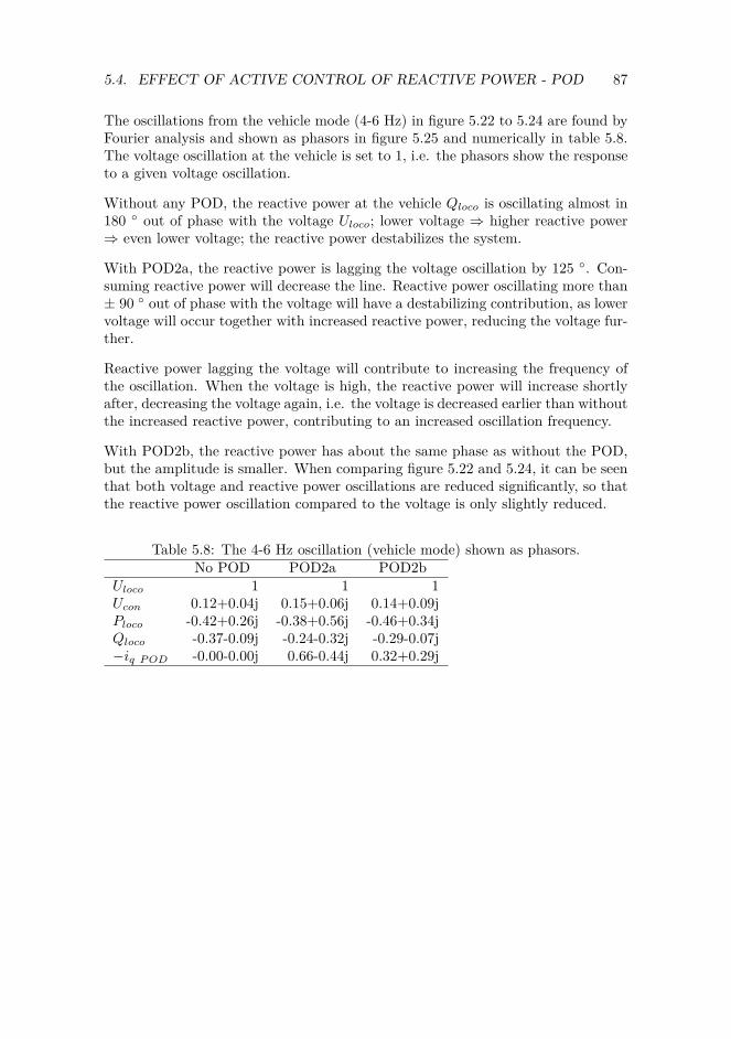
5.4. EFFECT OF ACTIVE CONTROL OF REACTIVE POWER - POD 87
The oscillations from the vehicle mode (4-6 Hz) in figure 5.22 to 5.24 are found byFourier analysis and shown as phasors in figure 5.25 and numerically in table 5.8.The voltage oscillation at the vehicle is set to 1, i.e. the phasors show the responseto a given voltage oscillation.
Without any POD, the reactive power at the vehicle Qloco is oscillating almost in180 out of phase with the voltage Uloco; lower voltage ⇒ higher reactive power⇒ even lower voltage; the reactive power destabilizes the system.
With POD2a, the reactive power is lagging the voltage oscillation by 125 . Con-suming reactive power will decrease the line. Reactive power oscillating more than± 90 out of phase with the voltage will have a destabilizing contribution, as lowervoltage will occur together with increased reactive power, reducing the voltage fur-ther.
Reactive power lagging the voltage will contribute to increasing the frequency ofthe oscillation. When the voltage is high, the reactive power will increase shortlyafter, decreasing the voltage again, i.e. the voltage is decreased earlier than withoutthe increased reactive power, contributing to an increased oscillation frequency.
With POD2b, the reactive power has about the same phase as without the POD,but the amplitude is smaller. When comparing figure 5.22 and 5.24, it can be seenthat both voltage and reactive power oscillations are reduced significantly, so thatthe reactive power oscillation compared to the voltage is only slightly reduced.
Table 5.8: The 4-6 Hz oscillation (vehicle mode) shown as phasors.No POD POD2a POD2b
Uloco 1 1 1Ucon 0.12+0.04j 0.15+0.06j 0.14+0.09jPloco -0.42+0.26j -0.38+0.56j -0.46+0.34jQloco -0.37-0.09j -0.24-0.32j -0.29-0.07j−iq POD -0.00-0.00j 0.66-0.44j 0.32+0.29j
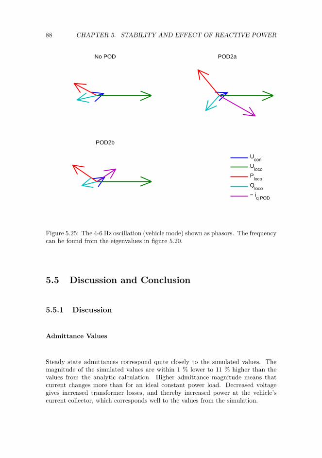
88 CHAPTER 5. STABILITY AND EFFECT OF REACTIVE POWER
No POD POD2a
POD2b
U
con
Uloco
Ploco
Qloco
− iq POD
Figure 5.25: The 4-6 Hz oscillation (vehicle mode) shown as phasors. The frequencycan be found from the eigenvalues in figure 5.20.
5.5 Discussion and Conclusion
5.5.1 Discussion
Admittance Values
Steady state admittances correspond quite closely to the simulated values. Themagnitude of the simulated values are within 1 % lower to 11 % higher than thevalues from the analytic calculation. Higher admittance magnitude means thatcurrent changes more than for an ideal constant power load. Decreased voltagegives increased transformer losses, and thereby increased power at the vehicle’scurrent collector, which corresponds well to the values from the simulation.

5.5. DISCUSSION AND CONCLUSION 89
Reasons for Increased Damping with Passive Control of Reactive Power
The vehicle gives a negative contribution to damping in a cases simulated, mostfor unity power factor, least for "minimum loss", dynamic φ.
The change of operating point from unity power factor to "minimum loss", static φgives a reduced voltage drop in the transmission, and thereby reduced voltage oscil-lations at both the converter station terminals and at the vehicle. But the voltageoscillation at the vehicle is in both cases about 1.5 times the voltage oscillation atthe converter station.
In the cases simulated here, the vehicle increases its real power when voltage de-creases, despite its constant real power control objective. This effect is also observedand commented by Danielsen [3], p. 120. Increasing vehicle power at decreasingvoltage causes increased transmission losses, as more power is to be transferred ata lower voltage, both causing increased current. Reduced voltage oscillations at thevehicle gives reduced oscillation in the vehicle real power, which reduces the lineloss oscillations, which again reduces oscillations in generator power and torque.
With "minimum loss" dynamic φ, reactive power is used in a way stabilizing thevoltage at the vehicle, where more reactive power is fed into the grid at lowervoltages, less at higher voltages. This reduces the voltage oscillations at the ve-hicle, such that the voltage oscillation is slightly smaller at the vehicle than atthe converter station. The voltage oscillations for a given speed oscillation aredecreased clearly from the other cases, both at the converter station and at thevehicle. A more stable vehicle voltage reduces the vehicle real power oscillations,which reduces the oscillations in generator power and torque.
Effect of Power Oscillation Damper - Traction
POD2a has some stabilizing effect on the rotary converter mode. The effect isvery similar to the effect obtain when changing from "minimum loss", static φto "minimum loss", dynamic φ. Increasing the gain reveals that the potential offurther stability improvement is limited, probably because the reactive power isstabilizing the voltage, and at the same time using the voltage magnitude as input.Keeping the voltage perfectly constant would require a finite output, while thevoltage oscillation at the input would be zero, i.e. an infinite gain.
Danielsen describes in [3], p. 141, how a power oscillation damper (POD) cancontrol the vehicle to produce or consume reactive power to keep the vehicle’scurrent magnitude, and thereby the transmission losses, constant during changingvoltage at the converter station terminals. This would give a constant real powerload at the converter station, eliminating the destabilizing impact of the vehicle.This control scheme is however not possible with the minimum loss settings, neitherwith passive ("minimum loss", dynamic φ) nor active control (POD) of reactive
90 CHAPTER 5. STABILITY AND EFFECT OF REACTIVE POWER
power. Reactive power is already used to keep losses at its minimum, and a minorchange of power factor will not influence the power loss. This can easily be shownby the criterion for finding the minimum of a function, the point where its derivativeequals 0 (dPloss
dφ = 0).
An illustration is shown in table 5.2. The simulations with "minimum loss", staticφ and "minimum loss", dynamic φ give virtually the same loss for a given voltageat the converter station, even though the reactive power differs approximately 9% between "minimum loss", static φ and "minimum loss", dynamic φ when theconverter station voltage is running at 16.665 kV or 16.335 kV.
It is observed that the POD2a yields better results for a vehicle operating at unitypower factor than at capacitive power factor. Danielsen obtains an eigenvalue of0.15 1/s ± j1.6 Hz at unity power factor, while at "minimum loss", dynamic φ, theeigenvalue is 0.13 1/s ± j1.6 Hz.
In addition to the POD2a, Danielsen describes two PODs acting on the real powerof the vehicle, called POD1a and POD1b. With unity power factor in steady state,these PODs give eigenvalues of -0.38 1/s ± j1.6 Hz and -0.43 1/s ± j1.6 Hz, whichis better damping than the rotary converter in no-load (-0.34 1/s ± j1.59 Hz) [3].
POD2b is not tuned to damp the rotary converter mode, and has very limitedeffect on this.
Effect of Power Oscillation Damper - No-load
POD2b has good effect on stabilizing the vehicle mode in no-load. The vehicle modeis fundamentally different from the rotary converter mode. The rotary convertermode is a mechanical oscillation, which can be influenced through the electrome-chanical torque of the generator, which is closely connected to real power, but onlyindirectly connected to reactive power. The vehicle mode is caused by the vehicledynamics and its response to the line voltage, and could also cause instability ina system fed by a stiff voltage source, with no rotary converter at all. The linevoltage is clearly affected by reactive power, and applied correctly, reactive powercan stabilize the line voltage, damping the oscillation.
The purpose of this chapter is not tuning the POD optimally, but describing theeffects of reactive power and its potential to improve stability. The oscillationfrequency, and then the frequency the POD should be tuned for, is depending onthe line length. The optimal tuning of a POD for no-load is probably not tuning itto give maximum damping at 200 km, where a very good damping may be obtained,but to tune it to increase the limit at which an acceptable stability in no-load maybe obtained to a maximum. A real vehicle should be tuned for stable operationat any power and line voltage likely to occur, which will probably require a moresophisticated tuning procedure than shown here.

5.5. DISCUSSION AND CONCLUSION 91
5.5.2 Conclusion
Traction - Damping of Rotary Converter Mode
The vehicle is found to destabilize the system in traction in all cases simulated, asthe electromagnetical load torque of the rotary converter oscillates more than 90 out of phase with the speed oscillations. The vehicle power increases slightly ata lower voltage; this effect is amplified by a long line as higher power transfer atlower line voltage increases the line loss.
Speed oscillations of a rotary converter is a mechanical oscillation, which is influ-enced by the electromagnetic torque of the rotary converters generator. Reactivepower is only indirectly coupled to electromagnetic torque, and can only in limiteddegree be used to stabilize speed oscillations of a rotary converter:
• Reactive power can be controlled to stabilize the voltage at the vehicle, reduc-ing the real power oscillations at the vehicle in traction. This is however onlyreducing the destabilizing impact, not creating a stabilizing impact. Whenvoltage magnitude is used as input for the reactive power controller, the ob-servability of the oscillations is reduced. This limits the possible stabilizingeffect of a reactive power controller.
• When operating at capacitive power factor to obtain minimum loss, the lineloss cannot be modulated to damp speed oscillations of a rotary converter.This reduces the potential for stabilizing such an oscillation by reactive power.
No-load - Damping of Vehicle Mode
In no-load, the vehicle control system and its response to the line voltage is foundto cause instability at long line lengths. Reactive power can be used to control theline voltage and thereby stabilize the system.
5.5.3 Further Work
Stability during regenerative braking is not investigated here. During regeneration,the vehicle is only allowed to operate at unity or inductive power factor to pre-vent an unacceptable voltage increase. This is not the operation giving minimumloss, and could thereby enable active damping through modulating the line loss byreactive power.
The control system structure and parameters of the vehicle in this thesis are copiedfrom Danielsen. The structure and most of the parameters are considered as fixed,and not discussed here. Better performance could probably be achieved by tuning

92 CHAPTER 5. STABILITY AND EFFECT OF REACTIVE POWER
parameters of the vehicle, together with the application of some kind of POD.Parameters should be tuned for stable operation over the entire operating range.A modification of the control structure could also be considered.
Stability analyses are in this thesis done on a system consisting of one vehicleand one rotary converter. To ensure stable operation in a real system, also morecomplex systems should be considered, consisting of several types of vehicles andstatic and rotary converters.

Chapter 6
Equivalent Admittance-based Dynamic Load Model
Assuming the manufacturer of a vehicle provided the input admittances as functionsof frequency and the steady state characteristics of the vehicle, a simulation ofsmall signal stability should be possible. This chapter describes the modellingof a dynamic load to be equivalent to the complete vehicle model, based on theoperating point and the vehicle admittance seen from the power system. Thedynamic behaviour of the equivalent model is compared to the behaviour of thecomplete model as found in chapter 5.
The equivalent load model will only be valid for the operating point (line voltageand vehicle power) at which the admittances are found.
The term "admittance-based" is used as the load model is defined by a response (achange of current) to a disturbance (change of voltage), and admittance is definedas current per voltage. The term "equivalent load model" is also used in this chapteras a shorter form of "equivalent admittance-based dynamic load model".
6.1 Modelling an Equivalent Admittance-based Dy-namic Load
The input admittances as functions of frequency of the vehicle model are found, asdescribed in section 5.2.2. The admittances are found for the operating points intable 5.1. The resulting admittances are shown in appendix C, figure C.2, C.4 andC.6. The admittances are found for the frequencies 0.01 Hz to 16 Hz. A load modelis to be implemented in DSL (Dynamic Simulation Language), being equivalent to
93

94CHAPTER 6. EQUIVALENT ADMITTANCE- BASED DYNAMIC LOAD MODEL
the vehicle at the given operating point regarding small signals at frequencies wellbelow the fundamental, 16 2/3 Hz.
6.1.1 Finding Transfer Function for Admittances
Curve Fitting by MatLab
The admittances of the equivalent load model are to be found on the form shown inequation 6.1, 6.2, 6.3 and 6.4. The factors b1.., b2.., b3.. and a1.., a2.., a3.. are foundby the MatLab function invfreqs. The numerical values are shown in appendixD.1. The invfreqs function solves the direct problem of minimizing the weightedsum of the squared error between the actual and the desired frequency responsepoints.
Ydd = ∆Id(s)∆Ud(s)
= b1dd · s2 + b2dd · s+ b3dd
a1dd · s2 + a2dd · s+ a3dd(6.1)
Yqd = ∆Iq(s)∆Ud(s)
= b1qd · s2 + b2qd · s+ b3qd
a1qd · s2 + a2qd · s+ a3qd(6.2)
Ydq = ∆Id(s)∆Uq(s)
= b1dq · s2 + b2dq · s+ b3dq
a1dq · s2 + a2dq · s+ a3dq(6.3)
Yqq = ∆Iq(s)∆Uq(s)
= b1qq · s2 + b2qq · s+ b3qq
a1qq · s2 + a2qq · s+ a3qq(6.4)
Frequency Weighting and Frequency Range
The admittances are found for frequency steps of 0.01 Hz (0.01 Hz, 0.02 Hz ... 16Hz). As a change from 0.01 Hz to 0.02 Hz is relatively a far larger change thanfrom 7.99 Hz to 8.00 Hz, the admittance for a given frequency is given a weightinversely proportional to its frequency, e.g. the weight at 0.02 Hz is set to 50 whilethe weight for 1 Hz is set to 1. The weight is used for minimizing the weighted sumof the squared error between the actual and the desired frequency response points.For the models of loaded vehicle starting curve fitting at 0.01 Hz, the weight for0.01 Hz is set to 1000000, to obtain a correct steady state value.
As the voltages and currents in the power system are modelled as phasors withfundamental frequency 16 2/3 Hz, the model is not valid above the fundamentalfrequency. The model is expected not to be fully valid at frequencies slightlybelow the fundamental; in most cases are therefore only frequencies below 8 Hzconsidered. The only exception is done for unity power factor, loaded vehicle. Inthis case curve fitting from 0.01 to 8 Hz gave a model with an obviously incorrectresponse, while curve fitting from 0.01 to 16 Hz gave a response fairly close to thecomplete vehicle model.
6.1. MODELLING AN EQUIVALENT ADMITTANCE-BASED DYNAMIC LOAD95
To obtain better fit around the frequencies of interest (eigenvalues at 1-5 Hz), it ischosen to simulate a set of models where the bandwidth for curve fitting is reduced.It is chosen to run curve fitting from 0.5 Hz to 6 Hz. The admittance for a givenfrequency is given a weight inversely proportional to its frequency. No frequencyis given weight of 1000000, as a steady state error is accepted for the bandwidth-reduced models. The frequency responses of the equivalent load models are showntogether with the complete model responses in appendix D.2 and D.3.
Suppression of Erroneous Data
The admittances at some frequencies are found to be far from the admittances ofneighbouring frequencies, forming "spikes" from an otherwise smooth curve. Thesespikes are assumed to be caused by numerical errors, and are given weight 0 whenfinding weighted least square error.
6.1.2 Implementation in SIMPOW
The load flow simulation (OPTPOW) is performed as for simulations with thecomplete vehicle model, as in chapter 5. When performing the dynamic simulation(DYNPOW), the dynamic vehicle model is replaced by an equivalent load model.The initial current I0 is taken from the OPTPOW (load flow) model of the vehicle,while the change of current ∆I due to voltage change ∆U is described by equations6.1 to 6.4, see figure 6.1. The 3-phase grid, the rotary converter station and theoverhead line is simulated by the same model as in chapter 5.
The equivalent load model is implemented as a load in SIMPOW written as aDSL-file. The source code can be found in appendix D.4.

96CHAPTER 6. EQUIVALENT ADMITTANCE- BASED DYNAMIC LOAD MODEL
Contact line
Single phase transformer
Three phase motor
Single phase generator
Three phase transformer
Feeding three phase network
MG
↓ [Yload]I0
Equivalent load
ΔI
U=U0+ ΔU
Figure 6.1: Circuit for simulation with the equivalent load model. The infrastruc-ture model is the complete model used in this thesis, while the vehicle model isreplaced by the equivalent load model. I0 is found from load flow, while ∆I iscontrolled by the admittances described by equation 6.1 to 6.4.
6.2. COMPLETE MODEL VS. EQUIVALENT LOAD MODEL 97
6.2 Complete Model vs. Equivalent Load Model
6.2.1 Eigenvalue Considerations
The eigenvalues of the system are shown in figure 6.2 (unity power factor), figure6.3 ("Minimum loss", static φ) and figure 6.4 ("Minimum loss", dynamic φ), com-paring the eigenvalues found with the complete vehicle model to the equivalentload models. The four pairs of eigenvalues having the lowest damping are shownin table 6.1, 6.2 and 6.3.
The four pairs of eigenvalues having the lowest damping show similar results forthe complete model and the equivalent load model, shown in table 6.3.
Both equivalent load models give eigenvalues relatively close to the complete vehiclemodel, though the bandwidth-reduced model (0.5-6 Hz) is in all cases clearly closerthan the model based on curve fitting at 0.01-8 Hz or 0.01-16 Hz. The rotaryconverter mode at 1.6 Hz is the least damped mode, and will dominate the responsein all cases. Particularly for unity power factor, there is a significant differencebetween the complete model and equivalent load model 0.01-16 Hz. The completemodel has a real part of 0.06 1/s which gives a damping of -0.53 %, while theequivalent load model 0.01-16 Hz has a real part of 0.43, which gives a damping of-4.2 %.

98CHAPTER 6. EQUIVALENT ADMITTANCE- BASED DYNAMIC LOAD MODEL
Unity power factor
−10 −8 −6 −4 −2 00
1
2
3
4
5
Re(λ) [1/s]
Im(λ
) [H
z]
Complete vehicle modelEquivalent admittance−based model, 0.01−16 HzEquivalent admittance−based model, 0.5−6 Hz
Figure 6.2: Eigenvalues with unity power factor for the complete model and theequivalent load models.
Table 6.1: Eigenvalues with unity power factor for the complete model and theequivalent load models. Eigenvalue numbers refer to the complete model, as intable B.1.
Eigenvalue [1/s], [Hz]Eigenvaluenumber
Completemodel
Equivalentload model0.01-16 Hz
Equivalentload model0.5-6 Hz
Main participant
17, 18 -5.49 ± j3.03 -5.92 ± j2.95 -5.55 ± j3.06 Vehicle19, 20 -4.83 ± j3.19 -4.83 ± j3.19 -4.83 ± j3.19 Motor exciter21, 22 -1.42 ± j2.28 -2.66 ± j1.72 -1.83 ± j2.26 Generator exciter25, 26 0.06 ± j1.64 0.43 ± j1.63 0.078± j1.65 Rotary converter

6.2. COMPLETE MODEL VS. EQUIVALENT LOAD MODEL 99
"Minimum Loss", Static φ
−10 −8 −6 −4 −2 00
1
2
3
4
5
Re(λ) [1/s]
Im(λ
) [H
z]
Complete vehicle modelEquivalent admittance−based model 0.01−8 HzEquivalent admittance−based model, 0.5−6 Hz
Figure 6.3: Eigenvalues with "minimum loss", static φ for the complete model andthe equivalent load models.
Table 6.2: Eigenvalues with "minimum loss", static φ for the complete model andthe equivalent load models. Eigenvalue numbers refer to the complete model, as intable B.2.
Eigenvalue [1/s], [Hz]Eigenvaluenumber
Completemodel
Equivalentload model0.01-8 Hz
Equivalentload model0.5-6 Hz
Main participant
17, 18 -5.72 ± j3.05 -6.40 ± j3.05 -6.03 ± j3.11 Vehicle19, 20 -4.83 ± j3.18 -4.83 ± j3.19 -4.83 ± j3.19 Motor exciter21, 22 -3.21 ± j2.54 -4.38 ± j2.48 -3.88 ± j2.54 Generator exciter25, 26 0.003 ± j1.61 0.053 ± j1.59 0.003 ± j1.60 Rotary converter

100CHAPTER 6. EQUIVALENT ADMITTANCE- BASED DYNAMIC LOAD MODEL
"Minimum Loss", Dynamic φ
−10 −8 −6 −4 −2 00
1
2
3
4
5
Re(λ) [1/s]
Im(λ
) [H
z]
Complete vehicle modelEquivalent admittance−based model 0.01−8 HzEquivalent admittance−based model, 0.5−6 Hz
Figure 6.4: Eigenvalues with "minimum loss", dynamic φ for the complete modeland the equivalent load models.
Table 6.3: Eigenvalues with "minimum loss", dynamic φ for the complete modeland the equivalent load models. Eigenvalue numbers refer to the complete model,as in table B.3.
Eigenvalue [1/s], [Hz]Eigenvaluenumber
Completemodel
Equivalentload model0.01-8 Hz
Equivalentload model0.5-6 Hz
Main participant
17, 18 -7.34 ± j3.10 -8.69 ± j3.29 -7.65 ± j3.31 Vehicle19, 20 -4.83 ± j3.19 -4.83 ± j3.18 -4.83 ± j3.19 Motor exciter21, 22 -4.75 ± j2.85 -4.80 ± j2.88 -4.78 ± j2.87 Generator exciter25, 26 -0.11 ± j1.60 -0.10 ± j1.59 -0.10 ± j1.59 Rotary converter

6.2. COMPLETE MODEL VS. EQUIVALENT LOAD MODEL 101
6.2.2 Time Domain Results
With "minimum loss", dynamic φ, the three least damped eigenvalues are verysimilar for the the equivalent load models and the full vehicle model. A timedomain simulation is performed to compare their response to a disturbance.
The system is excited with the same disturbance as in section 5.3.4, a 100 kW load
0 1 2 3 4 50.9135
0.914
0.9145
0.915
Time [s]
Vol
tage
[pu]
Complete vehicle modelEquivalent admittance−based model 0.01−8 HzEquivalent admittance−based model 0.5−6 Hz
0 1 2 3 4 5
0.5925
0.593
0.5935
Time [s]
Rea
l pow
er [p
u]
Figure 6.5: Voltage and real power at the vehicle, with "minimum loss", dynamicφ for the complete model and the equivalent load models.

102CHAPTER 6. EQUIVALENT ADMITTANCE- BASED DYNAMIC LOAD MODEL
is connected at the rotary converter 16.5 kV bus at t=-0.1 s, and disconnected att=0 s. The resulting voltage and real power at the vehicle’s current collector areshown in figure 6.5, together with the corresponding data from the simulation usingthe complete vehicle model.
The deviation between the models are most easily observed in the real power con-sumed by the vehicle, particularly in the first second. The equivalent admittancebased model 0.5-6 Hz follows the complete vehicle model closely at the first oscilla-tion down to 0.5924 pu, while the equivalent load model 0.01-8 Hz has a minimumvalue 0.5927 pu.
6.3 Long Line Stability Test - No-Load
The long line stability test is performed in no-load, i.e. the vehicle motor currentidcm = 0 to avoid a voltage collapse due to a high voltage drop. Depending on thecontrol structure of the vehicle, the input admittance will in most cases dependon the operating point of the vehicle (power and line voltage). When operatingthe vehicle in no-load, the operating point and thereby the input admittance isindependent of the line length. In order to simplify finding the stability limit fromthe load admittance and source impedance, the vehicle is supplied by a stiff voltagesource of 16.5 kV and a line with (0.19 + j0.21)Ω/km.
The different control schemes for reactive power described in section 3.2.1 and [5]all give unity power factor at 16.5 kV, and the choice of control scheme will haveno effect. Therefore, only the scheme for unity power factor is used in no-load.
6.3.1 Stability Limit by Simulation, Complete Model andEquivalent Load Models
The admittances of the vehicle in no-load are found as described in section 5.2.2,shown in figure C.8. Equivalent load models are made, based on curve fitting at0.01-8 Hz and 0.5-6 Hz. The admittances of the equivalent load models and thecomplete vehicle model are shown in figure D.7 and D.8.
The eigenvalues for the complete vehicle model and and the equivalent load modelsare shown in figure 6.6, for 200 km line length. The eigenvalues that are closest tocause instability are eigenvalues 9,10, -1.63 1/s ± j4.51 Hz in the complete vehiclemodel. For the equivalent load model, 0.5-6 Hz, two extra pairs of eigenvaluesappear at about -5.5 1/s ± j4.8 Hz.

6.3. LONG LINE STABILITY TEST - NO-LOAD 103
−20 −18 −16 −14 −12 −10 −8 −6 −4 −2 00
1
2
3
4
5
6
7
Re(λ) [1/s]
Im(λ
) [H
z]
Complete vehicle modelEquivalent admittance−based model 0.01−8 HzEquivalent admittance−based model, 0.5−6 Hz
Figure 6.6: Eigenvalues for the complete vehicle model and equivalent load models,found for frequencies 0.01-8 Hz and 0.5-6 Hz. The eigenvalues are found for 200km line length at no-load.
A data scanning of the eigenvalues 9,10 for the line length is performed for both thecomplete model and the equivalent load models, shown in figure 6.7. The stabilitylimit and the oscillation frequencies are shown in table 6.4. Both equivalent loadmodels indicate a stability limit 6-7 km different from the complete model, and anoscillation frequency about 0.2 Hz higher.

104CHAPTER 6. EQUIVALENT ADMITTANCE- BASED DYNAMIC LOAD MODEL
−5 −4 −3 −2 −1 0 14
4.2
4.4
4.6
4.8
5
5.2
5.4
160
180
200
220
240
260
160
180
200
220
240
260
160
180
200
220
240
260
Re(λ) [1/s]
Im(λ
) [H
z]
Complete vehicle modelEquivalent admittance−based model 0.01−8 HzEquivalent admittance−based model, 0.5−6 Hz
Figure 6.7: Data scanning for line length of the dominant eigenvalue for the com-plete vehicle model and equivalent load models, found for frequencies 0.01-8 Hzand 0.5-6 Hz.
Table 6.4: The stability limit for the complete vehicle model and equivalent loadmodels.Model Stability limit [km] Oscillation frequency [Hz]Complete vehicle model 239 4.25Equivalent load model,0.01-8 Hz
245 4.42
Equivalent load model,0.5-6 Hz
232 4.48

6.3. LONG LINE STABILITY TEST - NO-LOAD 105
6.3.2 Stability Limit from Impedance-based Modelling
The source impedance, which consist of only line impedance, and the load admit-tance are found for 200 km line length, shown in figure C.7 and C.8. The Nyquistcontour (N-1), equation 5.17, is found for line lengths from 200 to 300 km. Whencalculating N-1, the load admittance is constant, while the source impedance foundin the simulation for 200 km is increased proportionally with the line length. The
−12 −10 −8 −6 −4 −2 0−2
0
2
4
6
8
10
12Nyquist plot
Re(N−1)
Im(N
−1)
−1.5 −1 −0.5 0
−0.4
−0.2
0
0.2
0.4
0.6
Nyquist zoom
Re(N−1)
Im(N
−1) 3 Hz 4 Hz4.25 Hz
5 Hz
200 km220 km240 km260 km280 km300 km
Figure 6.8: Nyquist plot for line lengths from 200 to 300 km.
106CHAPTER 6. EQUIVALENT ADMITTANCE- BASED DYNAMIC LOAD MODEL
Nyquist contours are shown in figure 6.8. The curves for 200 and 220 km do notencircle (-1+j0) (stable system), while the curves for 240 km and above do (unsta-ble system). The curve for 239 km is not shown here but this would pass through(-1+j0) indicating a a marginally stable system at 239 km, the stability limit. Themarker for 240 km, 4.25 Hz is located very close to (-1+j0). This method for findingthe stability limit is further described and investigated in [11].
6.4 Discussion and Conclusion
6.4.1 Discussion
Equivalent Admittance-Based Dynamic Load Models vs. Complete Ve-hicle Model
The four least damped pairs of eigenvalues were found to be relatively similar withthe equivalent admittance-based dynamic load models (also called "equivalent loadmodel") compared to the complete vehicle model. One of these modes, 19,20, ismainly caused by the exciter of the rotary converter motor, and is earlier found verylittle affected by reactive power characteristics. Keeping this mode unchanged givesthereby little information regarding the vehicle behaviour. The two other modesare found two be clearly affected by the reactive power settings; that these modesare nearly unchanged indicate that the equivalent load model behaves similar tothe complete vehicle model.
The time domain simulations also show similar behaviour between the completemodel and the equivalent load models.
In all cases with loaded vehicle, the bandwidth-reduced models (0.5-6 Hz) havesmaller deviation from the complete model than the models based on curve fittingat 0.01-8 Hz or 0.01-16 Hz. For the long line stability test, performed in no-load,the two equivalent load models have about the same magnitude of deviation fromthe complete vehicle model.
Finding Stability Limit Directly from Load Admittance
The stability limit is found by the Nyquist contour from [Yload] and [Zsource] to239 km, the same value as found by scanning of eigenvalues. Also the oscillationfrequency is close to the value from eigenvalue scanning, 4.25 Hz.

6.4. DISCUSSION AND CONCLUSION 107
6.4.2 Conclusion
Equivalent load models can be made from the steady state characteristics of thevehicle, determining the operating point; and the admittance for the operatingpoint of interest, describing the dynamic behaviour. The equivalent load modelis an approximation, and does not behave exactly like the original vehicle. Curvefitting only in the frequency range where oscillations are expected to occur givesa dynamic response which is more similar to the original vehicle than a modelbased on curve fitting over a larger range. This is, however, assumed to reduce theaccuracy outside this frequency range, e.g. steady state characteristics.
To find whether a system is stable or not, finding the Nyquist contour from theoriginal admittance gives higher accuracy than a simulation the equivalent loadmodel, as the equivalent load model represents an approximation. On the otherhand, the Nyquist plot gives less information about damping and details about dy-namic behaviour than a simulation of the equivalent load model, finding eigenvaluesand time response.
6.4.3 Further Work
The equivalent load model is an approximation. Assuming a complete vehiclemodel is not available, only the admittance as function of frequency, a deeperunderstanding of the equivalent load modelling would be of interest in order todetermine and improve the accuracy of this approximation. Improving the accuracyis assumed to include higher order transfer functions and modified weighting offrequencies.
The equivalent load model is only valid at a specified operating point, i.e. linevoltage and vehicle power. By finding the admittances for several operating points,it should be possible to make an equivalent load model for any point within thisrange by interpolation.

108CHAPTER 6. EQUIVALENT ADMITTANCE- BASED DYNAMIC LOAD MODEL
Chapter 7
Conclusion
This thesis investigates the settings for reactive power during traction proposed inthe project done by the author fall 2010. In a system fed by rotary converters, thesettings are found to give a reduction of converter station loading and total loss ofa few percent in the best case, no significant change in the worst case.
The effect of reactive power on the system stability is investigate. During traction,the challenging issue regarding stability is speed oscillations of the rotary converter.Controlling reactive power, both through the steady state characteristics (passivecontrol) and through a power oscillation damper (POD) has a limited effect onthese oscillations. In no-load, the challenging issue regarding stability is oscillationscaused by the vehicle control system and its response to the line voltage. In thiscase, the steady state characteristics have no effect, but the POD improves dampingand stability limit significantly.
For simulation of a real vehicle, a complete simulation model of the vehicle and itscontrol system might not be available. In such a case, an equivalent load modelcan be made, based on the steady state characteristics and the input admittanceof the vehicle.
7.1 Loadflow - Capacity and Losses
In traffic simulation, the "minimum loss" settings reduced the converter losses atthe highest loaded converter station by 1.5 - 2.4 % compared to unity power factor.The highest current occurring is reduced by 0-3 %.
The total losses are reduced by 0.33 % with constant voltage characteristics, and0.21 % with 8 % decreasing characteristics, when changing from unity power factor
109

110 CHAPTER 7. CONCLUSION
to "minimum loss" settings of the load.
7.2 Stability
7.2.1 Rotary Converter Speed Oscillations in Traction
Speed oscillations of a rotary converter can only to a limited extent be influencedby controlling reactive power at the vehicle.
Danielsen implemented and tested power oscillation dampers (PODs) acting oneither real or reactive power. In this thesis only PODs acting on reactive power isused. PODs acting on real power damp rotary converter speed oscillations clearlybetter than PODs acting on reactive power.
The vehicle may be operated at capacitive power factor keeping the line loss at aminimum, but this mode of operation reduces the stabilizing effect of controllingreactive power. When the line loss is already at a minimum, it cannot be modulatedto damp oscillations by controlling reactive power.
7.2.2 Oscillations from Vehicle Control System in No-load
In no-load, the vehicle control system and its response to the line voltage is foundto cause instability at long line lengths. Reactive power can be used to control theline voltage and thereby stabilize the system.
7.3 Equivalent Load Modelling
An equivalent admittance-based load model can be made from the steady statecharacteristics of the vehicle, determining the operating point; and the admittancefor the operating point of interest, describing the dynamic behaviour. The equiva-lent admittance-based load model is an approximation, and does not behave exactlylike the original vehicle. Curve fitting only in the frequency range where oscilla-tions are expected to occur gives a dynamic response which is more similar to theoriginal vehicle than a model based on curve fitting over a larger range. This is,however, assumed to reduce the accuracy outside this frequency range, e.g. steadystate characteristics.
To find whether a system is stable or not, finding the Nyquist contour from theoriginal admittance gives higher accuracy than a simulation with the equivalentadmittance-based load model, as the equivalent admittance-based load model rep-resents an approximation. On the other hand, the Nyquist plot gives less informa-
7.4. FURTHER WORK 111
tion about damping and details about dynamic behaviour than a simulation of theequivalent load model, finding eigenvalues and time response.
7.4 Further Work
The settings for reactive power proposed in the fall project are calculated for asystem fed by one or more stiff voltage sources with the same voltage angle andmagnitude. A real optimization of the system should be a lot more complex, asit should consider both reactive power control at the vehicles and settings of theautomatic voltage regulators at the converter stations in a system consisting ofseveral vehicles and converter stations.
Stability is not analysed during regenerative braking. Capacitive power factor isnot allowed during regeneration, meaning that the transmission line will not beoperated at minimum loss. As loss is not at its minimum, it will vary with thepower factor of the vehicle, and reactive power may be used for modulating theline loss to damp oscillations.
The settings for power factor during regenerative braking described in section 3.2.2include ramps where the power factor should be changed as a function of voltage.It would be of interest how such ramps affect stability, and if there is a maximumslope of the ramps to ensure stability is not violated.
Equivalent load models may be modelled from the vehicle steady state character-istics and input admittance. Such a load model may be used in a time domainsimulation or eigenvalue calculation, without revealing the inner workings of thevehicle and its control system. It would be of interest to improve the accuracy ofthe equivalent admittance-based load modelling, and to estimate the accuracy ofsuch a model assuming the complete model is not available for comparison.

112 CHAPTER 7. CONCLUSION

References
[1] Steimel, A. (2008). Electric Traction - Motive Power and EnergySupply, Basics and Practical Experience. Oldenbourg Industriverlag,Munich.
[2] The Swedish Rail Administration/The Norwegian National RailAdministration (2007). Requirements on rolling stock in Nor-way and Sweden regarding EMC with the electrical infrastruc-ture and coordination with the power supply and other vehi-cles (BVS 543.19300/JD 590). Retrieved 18 August 2010 fromhttp://www.jernbaneverket.no/Documents/Marked/Infrastrukturens%20egenskaper/590/Vedlegg/T9004d00.pdf
[3] Danielsen, S (April 2010). Electric Traction Power System Stabil-ity - Low-frequency interaction between advanced rail vehicles anda rotary frequency converter, (Doctoral theses No. 2010:56, NTNU),NTNU Norwegian University of Science and Technology, Trondheim,Norway.
[4] Biedermann, N. (January 2010). Criteria for the voltagein railway power supply systems, (Thesis No. XR-EE-EME2010:002, KTH, 2010) KTH Royal Institute of Technol-ogy, Stockholm, Sweden. Retrieved 9 September 2010 fromhttps://eeweb01.ee.kth.se/upload/publications/reports/2010/XR-EE-EME_2010_002.pdf
[5] Toreid, E. (November 2010). Active Control of Reactive Power in aModern Electrical Rail Vehicle, (Special study). School of Environ-ment, Resources and Development, Asian Institute of Technology,Thailand.
[6] Performance description ... (Restricted). Document number3EGM015763D0045.
[7] CENELEC. (November 2004). European standard EN50163 - Rail-way Applications - Supply voltages of traction systems.
113

114 REFERENCES
[8] CENELEC. (August 2005). European standard EN50388 - Railwayapplications - Power supply and rolling stock - Technical Criteria forthe coordination between power supply (substation) and rolling stockto achieve interoperability.
[9] Martinsen, F. (October 2009). Spenningsregulatorinnstilling iroterende omformerstasjoner (Settings of Voltage Regulators in Ro-tary Converter Stations). The Norwegian National Rail Administra-tion, Oslo, Norway.
[10] Danielsen, S. (13 September 2010) Impedance-based study of low-frequency interaction between a rotary converter and an electric ve-hicle. The Norwegian National Rail Administration, Oslo, Norway.
[11] Pika, S. (August 2010)Understanding of the Stability Criterion fora Double-Feedback Loop System, Master thesis, Narvik UniversityCollege, Narvik, Norway.
[12] Skogestad, S. and Postlethwaite, I. (2005) Multivariable FeedbackControl - Analysis and Design John Wiley & Sons Ltd, West Sussex,England.
[13] Stensby, Ø. (14 January 2011) Email: "SV: Magnetiseringstap om-former" ("RE: Excitation losses converter")
[14] IEEE Std 421.5 - 2005 IEEE Recommended Practice for ExcitationSystem Models for Power System Stability Studies, IEEE Std 421.5-2005 (Revision of IEEE Std 421.5-1992). pp. 0_1-85, 2006.

Appendix A
Simulation ModelParameters
A.1 Train Model Parameters for Traffic Simula-tion
Table A.1: Train data used in simulation. Locomotive data from [6].Parameter Unit ValueTrain mass t 1000Dynamic mass1 t 1054.2Total length m 500A2 kN 12.07B2 kN/(km/h) 7.722 ·10−2
C2 kN/(km/h)2 3.735 ·10−3
Locomotive mass (adhesion mass) t 84Rated mechanical power MW 5.6Rated electrical power for traction MW 6.364Efficiency3 (lower at speed below 40 km/h) 1 0.88Auxillary electrical power and no-load losses kW 123.5Max tractive effort kN 300Max electric braking effort kN 240
1Dynamic mass is locomotive mass · 1.1 + cars’ mass · 1.05.2A, B and C are constants describing the train’s driving resistance, FR = A + B · v + C · v2.
FR is driving resistance in kN, v is speed in km/h.3Efficiency does not include auxiliary power
115

116 APPENDIX A. SIMULATION MODEL PARAMETERS
A.2 Power System Topology and Parameters
The dynamic simulation model is with a few exceptions the same model and pa-rameters as used by Danielsen [3].
A transportable synchronous-synchronous rotary frequency converter type ASEAQ38, having a rated power of 4 MVA, is feeding a single-track railway and onesingle rail vehicle. A single-line diagram in figure A.1 shows the steady-state powerflow for the reference case without reactive power control. The rotary converter
Figure A.1: Power system topology. The power flow shown is for the vehicleoperating at unity power factor.
is fed from a 66 kV 3-phase grid, having a short circuit power of 250 MVA at thetransformer upside, which are typical values in the Norwegian electrical tractionpower system [2]. The 3-phase grid is assumed to have a Z/R ratio of 4. Boththe motor and generator include exciters and automatic voltage controllers (AVR).The motor excitation adjusted so the reactive power at its terminal equals zero,which gives the reference voltage for the AVR. Furthermore, if necessary (here itwas not) the three-phase transformer tap-changer may be adjusted (in incrementsof 300 V) in order to keep the motor voltage as close as possible to 6.3 kV. Theline voltage at the single-phase transformer 15-kV side is controlled to be 16.5 kVwith a zero load-depending slope by use of the AVR. Data for the converter, thetransformers and the regulators are given in appendix A.3.
Between the rotary converter and the rail vehicle, there is 60 km of overheadcontact line. This length was chosen since it is the length of line for which a vehicleis required to operate stably in order to be accepted for operation in Norway andSweden [2]. The line impedance is (0.19 + j0.21)Ω/km.
The rail vehicle is based on exercise 17.8 by Steimel [1] and is further introducedand explained by Danielsen in [3]. It represents a 6.4 MW universal locomotivemeasured on wheel. This results in an electrical rating of 7.35 MW. The vehicle

A.3. ROTARY CONVERTER PARAMETERS 117
is operated on half of the rated power, i.e., 3.67 MW. The power and voltageat the vehicle’s current collector vary slightly between the simulation cases, asthe vehicle’s transformer loss and the line’s voltage drop depend on the vehicle’ssettings for reactive power. Further details about the vehicle are shown in appendixA.4.
A.3 Rotary Converter Parameters
A.3.1 Synchronous Machines
The rotary converter synchronous-machine parameters used in this thesis are givenin Table A.2. They have all been received from the former manufacturer of thesemachines, but the following changes, as described by Danielsen [3], apply:
• The inertia constant is increased by 5 % to take the exciters into account.
• The motor q-axis sub-transient reactance is increased by 42 % in order toadapt to the poor damping observed in reality.
Table A.2: Rotary converter synchronous machine parameters.Parameter Unit Motor Generator
SN Rated power MVA 4.4 4.0UN Rated voltage kV 6.3 4.0Xa Stator leakage reactance pu 0.11 0.096Ra Stator resistance pu 0.0033 0.00175Xd D-axis synchronous reactance pu 0.90 1.02X ′d D-axis transient reactance pu 0.24 0.12X ′′d D-axis sub-transient reactance pu 0.165 0.10Xq Q-axis synchronous reactance pu 0.40 0.47X ′q Q-axis transient reactance pu 0.40 0.47X ′′q Q-axis sub-transient reactance pu 0.34 0.11T ′d0 D-axis transient time constant s 4.0 8.6T ′′d0 D-axis sub-transient time constant s 0.04 0.08T ′′q0 Q-axis sub-transient time constant s 0.10 3.4H Inertia constant MWs/MVA 1.70 1.87RF Field winding resistance1 Ω 0.345 0.208IF0 No-load field current1 ( = 1 pu) A 110 148
The reactances are unsaturated and saturation in is not included in the model.The converter was originally designed for a continuous power of 4.0 MVA, but it
1From [13].

118 APPENDIX A. SIMULATION MODEL PARAMETERS
is later found to be dimesioned sufficiently for a continuous power of 5.8 MVA [9].Generator data are given for a pu base power of 4.0 MVA.
A.3.2 Transformers
The parameters for the transformers connecting the rotary converter to the respec-tive grids used in this thesis are given in Table A.3. The data are found in testprotocols.
Table A.3: Rotary-converter transformer parameters.Parameter Unit Motor Generator
SN Rated power MVA 4.4 4.0UN1 Rated voltage first winding kV 66 4.0UN2 Rated voltage second winding kV 6.3 16.6ER12 Short-circuit resistance pu 0.0054 0.014EX12 Short-circuit reactance pu 0.079 0.034
A.3.3 Automatic Voltage Regulator Parameters
The parameters for the exciters and ASEA YGUA automatic voltage regulatorsused in this thesis are given in Table A.4. The standard excitation system modelIEEE Type DC1A ’Excitation system with DC commutator exciter’ [14] is used.The background for the different parameter values are:
• TR is assumed to be half of the rectifier diode-bridge switching frequencyequal to a quarter of a fundamental period.
• KA is calculated by Stensby based on measurements from Landström.
• TA and TF are measured in Landström.
• KE is according to Högberg, zero due to rheostat adjustment.
• TE , V RMIN and V RMAX are found for the motor exciter by Stensby. Similarmeasurements and calculations are performed for generator exciter.
• KF is assumed to be equal to typical values as given by Andersson and Fouad.

A.4. VEHICLE MODEL PARAMETERS 119
Table A.4: Automatic voltage regulator parametersParameter Unit Motor Generator
TR Regulator input filter time constant s 0.005 0.015KA Regulator amplifier gain pu 382 382TA Regulator amplifier time constant s 0.11 0.11KE Exciter constant related to self-excited field pu 0.0 0.0TE Exciter time constant s 0.46 0.53KF Regulator stabiliser circuit gain pu 0.04 0.04TF Regulator stabiliser circuit time constant s 0.7 0.7V RMIN Min value of regulator output pu -2.9 -3.5V RMAX Max value of regulator output pu 2.9 3.5
No current (power) dependent voltage charateristic is used by Danielsen (RC =XC = 0 %), and this characteristic are used in the stability section of this thesis.In the load sharing section, there are used both a constant voltage characteristic(RC = XC = 0 %), and a characteristic with decreasing voltage for reactive power(RC = 0, XC = 8 %, with 16.5 kV, 5.8 MVA as pu base).
A.4 Vehicle Model Parameters
A.4.1 Electrical Component Values
The vehicle’s nominal power is 6.4 MW measured on wheel, which is used as thebase power for the per unit system. Taking losses and 5 % overload into accountas shown by Steimel [1], the rated power is 7.35 MVA. The line-side converter’sswitching frequency is 250 Hz.
The vehicle transformer and DC-link parameters are listed in Table A.5 and TableA.6, respectively.
Table A.5: Vehicle transformer parameters.Parameter Unit Value
SN Rated power MVA 7.35UN1 Rated voltage first winding kV 15UN2 Rated voltage second winding kV 1.568ER12 Short-circuit resistance pu 0.05EX12 Short-circuit reactance pu 0.333

120 APPENDIX A. SIMULATION MODEL PARAMETERS
Table A.6: Vehicle DC-link parameters.Parameter Unit Value
UdcN Rated voltage kV 2.8Cd DC-link capacitor mF 24.4C2 Second-harmonic filter capacitor mF 16.52L2 Second-harmonic filter inductor mH 1.375R2 Second-harmonic filter resistor mΩ 30
A.4.2 Control System Parameters
The vehicle control-system parameters used in the original model in this thesis arelisted in Table A.7. The per unit values are related to SBase = 6.4 MW and thetransformer secondary side voltage UBase = 1.568 kV.
Table A.7: Vehicle control system parameters.Parameter Unit Value
KuSOGI Voltage measurement SOGI gain pu 0.8KiSOGI Current measurement SOGI gain pu 3KpPLL Phase-locked loop gain pu 51TiPLL Phase-locked loop integration time s 0.079KpV C DC-link voltage controller gain pu 1.67TiV C DC-link voltage controller integra-
tion times 0.06
KpCC AC current controller gain pu 0.87TiCC AC current controller integration
times 180
TuDC DC-link voltage measurement filterbandwidth
Hz 100
TiDC Motor current measurement filterbandwidth
Hz 100
TfCPL Motor damping filter time constant s 0.15
-

Appendix B
Eigenvalue Tables
121

122 APPENDIX B. EIGENVALUE TABLES
Table B.1: Eigenvalues for unity power factorNo. Eigenvalue
[1/s], [Hz]Damping[%]
Main participation
13, 14 -21.01 ± 6.15 47.7 Vehicle AC voltage measurement 0.25Vehicle AC voltage measurement 0.51Vehicle PLL angle 0.52Vehicle PLL loop filter 0.17Vehicle voltage controller 0.10Vehicle AC current measurement 0.12
17, 18 -5.49 ± 3.03 27.7 Vehicle voltage controller 0.13Generator exciter field voltage 0.72
19, 20 -4.83 ± 3.19 23.4 Motor exciter field voltage 0.9821, 22 -1.42 ± 2.28 9.9 Vehicle DC-link 0.16
Vehicle DC-link 0.11Vehicle DC-link 0.13Generator d-axis damper winding flux 0.10Generator field winding flux 0.10Vehicle AC voltage measurement 0.38Vehicle voltage controller 0.44Vehicle d-axis current controller 0.11Generator exciter field voltage 0.16
25, 26 0.06 ± 1.64 -0.5 Motor power angle 0.52Motor speed 0.27Generator speed 0.27
29, 30 -4.56 ± 0.11 99.0 Vehicle DC-link 0.23Vehicle AC voltage measurement 0.10Vehicle AC voltage measurement 0.15Vehicle voltage controller 0.11Vehicle d-axis current controller 0.43Vehicle q-axis current controller 0.61
31, 32 -1.42 ± 0.35 53.8 Generator d-axis damper winding flux 0.28Generator speed 0.17Generator field winding flux 0.59Generator exciter field voltage 0.66
33, 34 -0.93 ± 0.16 66.9 Motor field winding flux 0.70Motor exciter regulator voltage 0.69

123
Table B.2: Eigenvalues for "minimum loss", static φNo. Eigenvalue
[1/s], [Hz]Damping[%]
Main participation
13, 14 -25.49 ± 6.37 53.7 Vehicle AC voltage measurement 0.33Vehicle AC voltage measurement 0.47Vehicle PLL angle 0.49Vehicle PLL loop filter 0.15Vehicle AC current measurement 0.13
17, 18 -5.72 ± 3.05 28.6 Vehicle AC voltage measurement 0.12Vehicle voltage controller 0.20Generator exciter field voltage 0.53
19, 20 -4.83 ± 3.18 23.5 Motor exciter field voltage 0.9821, 22 -3.21 ± 2.54 19.7 Vehicle DC-link 0.16
Vehicle DC-link 0.11Vehicle DC-link 0.10Vehicle AC voltage measurement 0.27Vehicle PLL angle 0.10Vehicle voltage controller 0.40Generator exciter field voltage 0.26
25, 26 3.10E-003 ± 1.61 0.0 Motor power angle 0.50Motor speed 0.25Generator speed 0.25
29, 30 -4.82 ± 0.13 98.6 Vehicle DC-link 0.21Vehicle AC voltage measurement 0.11Vehicle d-axis current controller 0.40Vehicle q-axis current controller 0.45
31, 32 -1.25 ± 0.31 54.6 Generator d-axis damper winding flux 0.25Generator speed 0.10Generator field winding flux 0.56Generator exciter field voltage 0.68
33, 34 -0.93 ± 0.16 67.2 Motor field winding flux 0.70Motor exciter regulator voltage 0.70

124 APPENDIX B. EIGENVALUE TABLES
Table B.3: Eigenvalues for "minimum loss", dynamic φNo. Eigenvalue
[1/s], [Hz]Damping[%]
Main participation
12, 13 -25.95 ± 9.13 41.2 Overhead lineVehicle transformer 0.13Vehicle AC voltage measurement 0.55Vehicle AC voltage measurement 0.38Vehicle PLL angle 0.27Vehicle AC current measurement 0.27Vehicle AC current measurement 0.13
17, 18 -7.34 ± 3.10 35.3 Vehicle DC-link 0.21Vehicle DC-link 0.14Vehicle AC voltage measurement 0.18Vehicle PLL angle 0.18Vehicle PLL loop filter 0.11Vehicle voltage controller 0.43Vehicle AC current measurement 0.10
19, 20 -4.83 ± 3.19 23.4 Motor exciter field voltage 0.9821, 22 -4.75 ± 2.85 25.6 Vehicle voltage controller 0.13
Generator exciter field voltage 0.8625, 26 -0.11 ± 1.60 1.1 Motor power angle 0.51
Motor speed 0.25Generator speed 0.25
29, 30 -5.16 ± 0.10 99.2 Vehicle DC-link 0.19Vehicle d-axis current controller 0.40Vehicle q-axis current controller 0.43
31, 32 -0.94 ± 0.24 52.4 Generator d-axis damper winding flux 0.21Generator field winding flux 0.51Generator exciter field voltage 0.65
33, 34 -0.93 ± 0.16 67.2 Motor field winding flux 0.70Motor exciter regulator voltage 0.70

Appendix C
Impedance and AdmittancePlots
125

126 APPENDIX C. IMPEDANCE AND ADMITTANCE PLOTS
10−2
10−1
100
101
10−2
100
102
|Z| [
pu]
f [Hz]
Unity Power Factor
Zdd Zqd Zdq Zqq
arg(
Y)
[deg
]
f [Hz]10
−210
−110
010
1−180
−90
0
90
180
Figure C.1: Power supply impedance from case "Unity power factor".
10−2
10−1
100
101
10−10
100
1010
|Y| [
pu]
f [Hz]
Unity Power Factor
Ydd Yqd Ydq Yqq
arg(
Y)
[deg
]
f [Hz]10
−210
−110
010
1−180
−90
0
90
180
Figure C.2: Load admittance from case "Unity power factor".

127
10−2
10−1
100
101
10−2
100
102
|Z| [
pu]
f [Hz]
"Minimum loss", static φ
Zdd Zqd Zdq Zqq
arg(
Y)
[deg
]
f [Hz]10
−210
−110
010
1−180
−90
0
90
180
Figure C.3: Power supply impedance from case "Minimum loss", static φ.
10−2
10−1
100
101
10−0.9
100.2
|Y| [
pu]
f [Hz]
"Minimum loss", static φ
Ydd Yqd Ydq Yqq
arg(
Y)
[deg
]
f [Hz]10
−210
−110
010
1−180
−90
0
90
180
Figure C.4: Load admittance from case "Minimum loss", static φ.

128 APPENDIX C. IMPEDANCE AND ADMITTANCE PLOTS
10−2
10−1
100
101
10−2
100
102
|Z| [
pu]
f [Hz]
"Minimum loss", dynamic φ
Zdd Zqd Zdq Zqq
arg(
Y)
[deg
]
f [Hz]10
−210
−110
010
1−180
−90
0
90
180
Figure C.5: Power supply impedance from case "Minimum loss", dynamic φ.
10−2
10−1
100
101
100
|Y| [
pu]
f [Hz]
"Minimum loss", dynamic φ
Ydd Yqd Ydq Yqq
arg(
Y)
[deg
]
f [Hz]10
−210
−110
010
1−180
−90
0
90
180
Figure C.6: Load admittance from case "Minimum loss", dynamic φ.

129
10−2
10−1
100
101
1
1.5
2|Z
| [pu
]
f [Hz]
Unity Power Factor − No−Load
Zdd Zqd Zdq Zqq
arg(
Y)
[deg
]
f [Hz]10
−210
−110
010
1−180
−90
0
90
180
Figure C.7: Power supply impedance in no-load, stiff voltage source, 200 km line.
10−2
10−1
100
101
10−12
10−8
10−4
100
|Y| [
pu]
f [Hz]
Unity Power Factor − No−Load
Ydd Yqd Ydq Yqq
arg(
Y)
[deg
]
f [Hz]10
−210
−110
010
1−180
−90
0
90
180
Figure C.8: Load admittance in no-load, unity power factor.

130 APPENDIX C. IMPEDANCE AND ADMITTANCE PLOTS

Appendix D
Equivalent Load
D.1 Equivalent Load Parameters
131

132 APPENDIX D. EQUIVALENT LOAD
Table D.1: Parameters for transfer functions describing the equivalent load, foroperating points from table 5.1 and at no-load at 16.5 kV.Parameter Simulation case
Unity powerfactor, 0.01-16Hz
"Minimumloss", static φ,0.01-8 Hz
"Minimumloss", dynamicφ, 0.01-8 Hz
No-load,0.01-8 Hz
b1dd 1.59485 1.05291 0.946526 0.823758b2dd -77.2403 -50.2389 -51.0383 -12.2242b3dd -628.033 -687.341 -697.44 11.64b1qd -0.244924 0.00497904 -0.0432643 0.00939448b2qd 20.2574 -8.75212 -84.0027 0.627388b3qd -0.0657475 -150.133 -1055.65 0.395931b1dq 0.163352 0.0802644 0.0803873 -0.00983501b2dq 4.78589 -9.1714 -9.17628 -0.62376b3dq -0.0525647 -140.742 -140.691 -0.421945b1qq 1.34009 0.941673 0.941606 1.35809b2qq 34.0905 20.7327 20.7344 -0.81361b3qq 2632.12 1242.81 1242.34 0.601939a1dd 1 1 1 1a2dd 65.2998 49.5733 50.3289 49.8551a3dd 689.856 903.112 884.288 1737.99a1qd 1 1 1 1a2qd 105.026 28.06 56.9394 11.9967a3qd 8448.02 721.289 612.462 1706.82a1dq 1 1 1 1a2dq 53.509 33.2391 33.2585 12.0383a3dq 11978.7 724.824 724.564 1691.59a1qq 1 1 1 1a2qq 77.2624 46.7774 46.7939 63.6794a3qq 3122.74 1750.5 1749.85 239.965

D.1. EQUIVALENT LOAD PARAMETERS 133
Table D.2: Parameters for transfer functions describing the bandwidth-reducedequivalent load, for operating points from table 5.1 and at no-load at 16.5 kV.Parameter Simulation case
Unity powerfactor, 0.5-6Hz
"Minimumloss", static φ,0.5-6 Hz
"Minimumloss", dynamicφ, 0.5-6 Hz
No-load, 0.5-6Hz
b1dd 0.923636 0.919521 0.822807 0.498749b2dd -52.6472 -45.8278 -46.2618 -7.74997b3dd -710.338 -601.305 -623.877 20.0456b1qd 0.0658099 0.000641705 -0.144582 0.0119592b2qd 1.04935 -9.511 -74.3714 0.168518b3qd -0.496844 -115.077 -1747.45 0.817123b1dq 0.0157188 0.0811354 0.0811758 -0.0124268b2dq -0.58692 -8.47684 -8.47771 -0.163302b3dq -1.05112 -129.852 -129.893 -0.874087b1qq 0.697737 0.751806 0.75199 1.32268b2qq 9.18958 10.102 10.1109 -0.82489b3qq 675.387 783.103 783.49 1.85008a1dd 1 1 1 1a2dd 43.2238 43.7786 44.5145 29.3209a3dd 818.187 834.674 826.749 1310.14a1qd 1 1 1 1a2qd 22.1258 28.5163 57.598 10.8976a3qd 725.282 611.743 1042.11 954.488a1dq 1 1 1 1a2dq 21.8746 30.5964 30.6038 11.0702a3dq 579.383 706.403 706.449 938.646a1qq 1 1 1 1a2qq 18.378 22.3447 22.3619 61.6969a3qq 819.086 1134.42 1134.99 248.658

134 APPENDIX D. EQUIVALENT LOAD
D.2 Admittance of Equivalent Load - Loaded Ve-hicle
Admittance as function of frequency for the complete vehicle model, shown withdots, and the admittance-based equivalent load shown as lines. The control schemefor reactive power and frequency range are given in the caption for each figure.

D.2. ADMITTANCE OF EQUIVALENT LOAD - LOADED VEHICLE 135
10−2
10−1
100
101
10−4
10−2
100
102
Frequency [Hz]
Mag
nitu
de
Ydd Yqd Ydq Yqq
10−2
10−1
100
101
−200
0
200
Frequency [Hz]
Ang
le [° ]
Figure D.1: Unity power factor, curve fitting performed from 0.01 to 16 Hz.
10−2
10−1
100
101
10−4
10−2
100
102
Frequency [Hz]
Mag
nitu
de
Ydd Yqd Ydq Yqq
10−2
10−1
100
101
−200
0
200
Frequency [Hz]
Ang
le [° ]
Figure D.2: Unity power factor, curve fitting performed from 0.5 to 6 Hz.
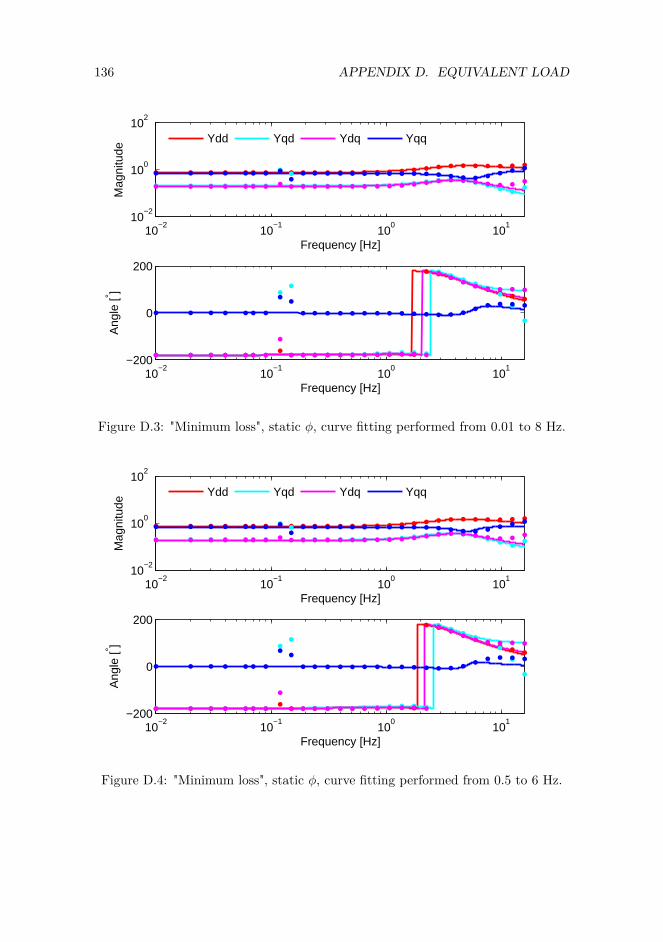
136 APPENDIX D. EQUIVALENT LOAD
10−2
10−1
100
101
10−2
100
102
Frequency [Hz]
Mag
nitu
de
Ydd Yqd Ydq Yqq
10−2
10−1
100
101
−200
0
200
Frequency [Hz]
Ang
le [° ]
Figure D.3: "Minimum loss", static φ, curve fitting performed from 0.01 to 8 Hz.
10−2
10−1
100
101
10−2
100
102
Frequency [Hz]
Mag
nitu
de
Ydd Yqd Ydq Yqq
10−2
10−1
100
101
−200
0
200
Frequency [Hz]
Ang
le [° ]
Figure D.4: "Minimum loss", static φ, curve fitting performed from 0.5 to 6 Hz.

D.2. ADMITTANCE OF EQUIVALENT LOAD - LOADED VEHICLE 137
10−2
10−1
100
101
10−0.8
100.2
Frequency [Hz]
Mag
nitu
de
Ydd Yqd Ydq Yqq
10−2
10−1
100
101
−200
0
200
Frequency [Hz]
Ang
le [° ]
Figure D.5: "Minimum loss", dynamic φ, curve fitting performed from 0.01 to 8Hz.
10−2
10−1
100
101
10−0.8
100.2
Frequency [Hz]
Mag
nitu
de
Ydd Yqd Ydq Yqq
10−2
10−1
100
101
−200
0
200
Frequency [Hz]
Ang
le [° ]
Figure D.6: "Minimum loss", dynamic φ, curve fitting performed from 0.5 to 6 Hz.

138 APPENDIX D. EQUIVALENT LOAD
D.3 Admittance of Equivalent Load - No-Load
Admittance as function of frequency for the complete vehicle model, shown withdots, and the admittance-based equivalent load shown as lines. The control schemefor reactive power have no effect in no-load, only unity power factor is used. Thefrequency range at which curve fitting is performed is given in the caption for eachfigure.

D.3. ADMITTANCE OF EQUIVALENT LOAD - NO-LOAD 139
10−2
10−1
100
101
10−3
100
Frequency [Hz]
Mag
nitu
de
Ydd Yqd Ydq Yqq
10−2
10−1
100
101
−200
0
200
Frequency [Hz]
Ang
le [° ]
Figure D.7: Unity power factor, no-load, curve fitting performed from 0.01 to 8Hz.
10−2
10−1
100
101
10−3
100
Frequency [Hz]
Mag
nitu
de
Ydd Yqd Ydq Yqq
10−2
10−1
100
101
−200
0
200
Frequency [Hz]
Ang
le [° ]
Figure D.8: Unity power factor, no-load, curve fitting performed from 0.5 to 6 Hz.

140 APPENDIX D. EQUIVALENT LOAD
D.4 DSL-file for Admittance Based Load Model
PROCESS EQLOADMINDYN(BUS,IR0,II0)REAL IR0,II0,UR0/*/,UI0/*/,URE,UIMREAL XDD,DXDD,DDXDD,IDDSTATE XDD,DXDDREAL XDQ,DXDQ,DDXDQ,IDQSTATE XDQ,DXDQREAL XQD,DXQD,DDXQD,IQDSTATE XQD,DXQDREAL XQQ,DXQQ,DDXQQ,IQQSTATE XQQ,DXQQ
PLOT XDD,DXDD,IDD,IDQ,IQD,IQQ
REAL b1dd/0.94652633/REAL b2dd/-51.038308/REAL b3dd/-697.44033/REAL b1dq/0.080387254/REAL b2dq/-9.1762819/REAL b3dq/-140.69068/REAL b1qd/-0.043264266/REAL b2qd/-84.002654/REAL b3qd/-1055.6519/REAL b1qq/0.94160579/REAL b2qq/20.734382/REAL b3qq/1242.3367/
REAL a1dd/1/REAL a2dd/50.328897/REAL a3dd/884.28846/REAL a1dq/1/REAL a2dq/33.25846/REAL a3dq/724.56386/REAL a1qd/1/REAL a2qd/56.93943/REAL a3qd/612.46198/REAL a1qq/1/REAL a2qq/46.793905/REAL a3qq/1749.8464/
EXTERNAL IR0,II0AC BUSAC_CURRENT I/BUS/

D.4. DSL-FILE FOR ADMITTANCE BASED LOAD MODEL 141
IF (TRANSTA) THENIF(START) THENUR0=UPRE(BUS)UI0=UPIM(BUS)IPRE(I)=IR0IPIM(I)=II0
ELSE!!YDD d-axis current, d-axis voltageURE=UPRE(BUS)-UR0UIM=UPIM(BUS)-UI0
DXDD: .D/DT.XDD = DXDDXDD: .D/DT.DXDD*A1DD=URE-DXDD*A2DD-XDD*A3DDIDD=B1DD*.D/DT.DXDD+B2DD*DXDD+XDD*B3DD
DXDQ: .D/DT.XDQ = DXDQXDQ: .D/DT.DXDQ*A1DQ=UIM-DXDQ*A2DQ-XDQ*A3DQIDQ=B1DQ*.D/DT.DXDQ+B2DQ*DXDQ+XDQ*B3DQ
DXQD: .D/DT.XQD = DXQDXQD: .D/DT.DXQD*A1QD=URE-DXQD*A2QD-XQD*A3QDIQD=B1QD*.D/DT.DXQD+B2QD*DXQD+XQD*B3QD
DXQQ: .D/DT.XQQ = DXQQXQQ: .D/DT.DXQQ*A1QQ=UIM-DXQQ*A2QQ-XQQ*A3QQIQQ=B1QQ*.D/DT.DXQQ+B2QQ*DXQQ+XQQ*B3QQ
IPRE(I)=IR0-IDD-IDQIPIM(I)=II0-IQD-IQQ
ENDIF !!End startENDIF !!Virker bare i TRANSTA, END - IF (TRANSTA) THENEND