action recognition using particle flow...
TRANSCRIPT

ACTION RECOGNITION USING PARTICLE FLOW FIELDS
by
KISHORE K. REDDYB.S. Jawaharlal Nehru Technological University, India
M.S. Fachhochschule Sudwestfalen, Germany
A dissertation submitted in partial fulfillment of the requirementsfor the degree of Doctor of Philosophy
in the Department of Electrical Engineering and Computer Sciencein the College of Engineering and Computer Science
at the University of Central FloridaOrlando, Florida
Summer Term2012
Major Professor: Mubarak Shah

c© 2012 KISHORE K. REDDY
ii

ABSTRACT
In recent years, research in human action recognition has advanced on multiple fronts
to address various types of actions including simple, isolated actions in staged data (e.g., KTH
dataset), complex actions (e.g., Hollywood dataset), and naturally occurring actions in surveil-
lance videos (e.g, VIRAT dataset). Several techniques including those based on gradient, flow,
and interest-points, have been developed for their recognition. Most perform very well in stan-
dard action recognition datasets, but fail to produce similar results in more complex, large-scale
datasets. Action recognition on large categories of unconstrained videos taken from the web
is a very challenging problem compared to datasets like KTH (six actions), IXMAS (thirteen
actions), and Weizmann (ten actions). Challenges such as camera motion, different viewpoints,
huge interclass variations, cluttered background, occlusions, bad illumination conditions, and
poor quality of web videos cause the majority of the state-of-the-art action recognition ap-
proaches to fail. An increasing number of categories and the inclusion of actions with high
confusion also increase the difficulty of the problem.
The approach taken to solve this action recognition problem depends primarily on the
dataset and the possibility of detecting and tracking the object of interest. In this dissertation, a
new method for video representation is proposed and three new approaches to perform action
recognition in different scenarios using varying prerequisites are presented. The prerequisites
have decreasing levels of difficulty to obtain: 1) Scenario requires human detection and track-
iii

ing to perform action recognition; 2) Scenario requires background and foreground separation
to perform action recognition; and 3) No pre-processing is required for action recognition.
First, we propose a new video representation using optical flow and particle advection.
The proposed “Particle Flow Field” (PFF) representation has been used to generate motion
descriptors and tested in a Bag of Video Words (BoVW) framework on the KTH dataset. We
show that particle flow fields has better performance than other low-level video representations,
such as 2D-Gradients, 3D-Gradients and optical flow.
Second, we analyze the performance of the state-of-the-art technique based on the his-
togram of oriented 3D-Gradients in spatio temporal volumes, where human detection and track-
ing are required. We use the proposed particle flow field and show superior results compared
to the histogram of oriented 3D-Gradients in spatio temporal volumes.
The proposed method, when used for human action recognition, just needs human de-
tection and does not necessarily require human tracking and figure centric bounding boxes. It
has been tested on KTH (six actions), Weizmann (ten actions), and IXMAS (thirteen actions,
4 different views) action recognition datasets.
Third, we propose using the scene context information obtained from moving and sta-
tionary pixels in the key frames, in conjunction with motion descriptors obtained using Bag of
Words framework, to solve the action recognition problem on a large (50 actions) dataset with
videos from the web. We perform a combination of early and late fusion on multiple features to
handle the huge number of categories. We demonstrate that scene context is a very important
feature for performing action recognition on huge datasets.
iv

The proposed method needs separation of moving and stationary pixels, and does not
require any kind of video stabilization, person detection, or tracking and pruning of features.
Our approach obtains good performance on a huge number of action categories. It has been
tested on the UCF50 dataset with 50 action categories, which is an extension of the UCF
YouTube Action (UCF11) Dataset containing 11 action categories. We also tested our approach
on the KTH and HMDB51 datasets for comparison.
Finally, we focus on solving practice problems in representing actions by bag of spatio
temporal features (i.e. cuboids), which has proven valuable for action recognition in recent
literature. We observed that the visual vocabulary based (bag of video words) method suffers
from many drawbacks in practice, such as: (i) It requires an intensive training stage to obtain
good performance; (ii) it is sensitive to the vocabulary size; (iii) it is unable to cope with
incremental recognition problems; (iv) it is unable to recognize simultaneous multiple actions;
(v) it is unable to perform recognition frame by frame.
In order to overcome these drawbacks, we propose a framework to index large scale
motion features using Sphere/Rectangle-tree (SR-tree) for incremental action detection and
recognition. The recognition comprises of the following two steps: 1) recognizing the local
features by non-parametric nearest neighbor (NN), and 2) using a simple voting strategy to
label the action. It can also provide localization of the action. Since it does not require fea-
ture quantization it can efficiently grow the feature-tree by adding features from new training
actions or categories. Our method provides an effective way for practical incremental action
recognition. Furthermore, it can handle large scale datasets because the SR-tree is a disk-based
v

data structure. We tested our approach on two publicly available datasets, the KTH dataset and
the IXMAS multi-view dataset, and achieved promising results.
vi

To my parents,
brother, and sister,
for their love and sacrifices.
∼
To my beloved wife,
for her support.
vii

ACKNOWLEDGMENTS
I would like to express my sincere thanks to my advisor Dr. Mubarak Shah for giving
me an opportunity to work in Computer Vision Lab. This work would not have been possible
without his guidance, encouragement, advice and support.
I am grateful to Dr. Lei Wei, Dr. Gita Sukthankar, and Dr. Brian Moore for serving on
my committee. I would also like to thank my mentors, Dr. Naresh Cuntoor and Dr. Amitha
Perera for their help during my summer internship at Kitware. I am grateful to the support
given by Shreya Trivedi, Dr. Max Poole and Dr. Patricia Bishop during the toughest times in
my life. I sincerely thank Dr. Aman Behal for supporting me in the early years of my Ph.D.
I would also like to thank my friends and colleagues, Suraj Vemuri, Vaibhav Thakore,
Jingen Liu, Jonathan Poock , Berkan Solmaz, Enrique G. Ortiz, Vladimir Reilly, Imran Saleemi,
Subhabrata Bhattacharya, Mikel Rodriguez and several others who made my stay in Orlando
and work at Computer Vision Lab memorable.
Special thanks to my parents, Tatayya Babu and Jaya Lakshmi for their love, support
and encouragement throughout my life. I am also thankful to my brother Kiran Kumar, and my
sister Swapna for their love and support. Above all, I would like to thank my wife Deepti for
her personal support and patience at all times.
viii

TABLE OF CONTENTS
LIST OF FIGURES . . . . . . . . . . . . . . . . . . . . . . . . . . . . . . . . . . . xiii
LIST OF TABLES . . . . . . . . . . . . . . . . . . . . . . . . . . . . . . . . . . . xvii
CHAPTER 1: INTRODUCTION . . . . . . . . . . . . . . . . . . . . . . . . . . . . 1
1.1 Overview and Motivation . . . . . . . . . . . . . . . . . . . . . . . . . . . . . 2
1.2 Contributions . . . . . . . . . . . . . . . . . . . . . . . . . . . . . . . . . . . 4
1.2.1 Particle Flow Fields to represent videos . . . . . . . . . . . . . . . . . 5
1.2.2 3D - Spatio Temporal Volumes . . . . . . . . . . . . . . . . . . . . . . 6
1.2.3 Scene context in web videos . . . . . . . . . . . . . . . . . . . . . . . 7
1.2.4 Incremental Action Recognition Using Feature-Trees . . . . . . . . . . 8
1.2.5 Challenging Datasets . . . . . . . . . . . . . . . . . . . . . . . . . . . 9
1.3 Organization of the Thesis . . . . . . . . . . . . . . . . . . . . . . . . . . . . 10
CHAPTER 2: LITERATURE REVIEW . . . . . . . . . . . . . . . . . . . . . . . . . 11
2.1 Low-Level Representation of Video . . . . . . . . . . . . . . . . . . . . . . . 13
2.2 Action Recognition in Large Realistic Datasets . . . . . . . . . . . . . . . . . 15
2.3 Action Recognition using Tree Data Structures . . . . . . . . . . . . . . . . . 16
ix

CHAPTER 3: PARTICLE FLOW FIELD . . . . . . . . . . . . . . . . . . . . . . . . 19
3.1 Introduction . . . . . . . . . . . . . . . . . . . . . . . . . . . . . . . . . . . . 19
3.2 Low-Level Video Representation . . . . . . . . . . . . . . . . . . . . . . . . . 20
3.2.1 Normalized Pixel Values . . . . . . . . . . . . . . . . . . . . . . . . . 20
3.2.2 Gradients . . . . . . . . . . . . . . . . . . . . . . . . . . . . . . . . . 20
3.2.3 Optical Flow . . . . . . . . . . . . . . . . . . . . . . . . . . . . . . . 22
3.2.4 Particle Flow (Particle Velocity) . . . . . . . . . . . . . . . . . . . . . 23
3.3 Experiments . . . . . . . . . . . . . . . . . . . . . . . . . . . . . . . . . . . . 25
3.4 Summary . . . . . . . . . . . . . . . . . . . . . . . . . . . . . . . . . . . . . 27
CHAPTER 4: 3D - SPATIO TEMPORAL VOLUMES . . . . . . . . . . . . . . . . . 29
4.1 Introduction . . . . . . . . . . . . . . . . . . . . . . . . . . . . . . . . . . . . 29
4.2 Histogram of Oriented 3D Spatiotemporal Gradients (3D-STHOG) . . . . . . . 31
4.3 Histogram of Oriented Particle Flow Fields (3D-STHOPFF) . . . . . . . . . . 34
4.4 Experiments using 3D-STHOG . . . . . . . . . . . . . . . . . . . . . . . . . . 35
4.4.1 UT-Tower Dataset . . . . . . . . . . . . . . . . . . . . . . . . . . . . 35
4.4.1.1 Sensitivity to Scale . . . . . . . . . . . . . . . . . . . . . . 36
4.4.1.2 Sensitivity to Frame Rate . . . . . . . . . . . . . . . . . . . 38
4.4.1.3 Sensitivity to Translation (Misalignment) . . . . . . . . . . . 38
4.4.2 VIRAT Ground Video Dataset . . . . . . . . . . . . . . . . . . . . . . 40
x

4.4.3 VIRAT Aerial Video Dataset . . . . . . . . . . . . . . . . . . . . . . . 44
4.4.4 IXMAS Dataset . . . . . . . . . . . . . . . . . . . . . . . . . . . . . . 46
4.4.5 KTH and Weizmann Datasets . . . . . . . . . . . . . . . . . . . . . . 46
4.5 Experiments using 3D-STHOPFF . . . . . . . . . . . . . . . . . . . . . . . . 47
4.6 Summary . . . . . . . . . . . . . . . . . . . . . . . . . . . . . . . . . . . . . 48
CHAPTER 5: SCENE CONTEXT FOR WEB VIDEOS . . . . . . . . . . . . . . . . 49
5.1 Introduction . . . . . . . . . . . . . . . . . . . . . . . . . . . . . . . . . . . . 49
5.2 Analysis on large scale dataset . . . . . . . . . . . . . . . . . . . . . . . . . . 51
5.2.1 Effect of increasing the action classes . . . . . . . . . . . . . . . . . . 53
5.3 Scene Context descriptor . . . . . . . . . . . . . . . . . . . . . . . . . . . . . 54
5.3.1 How discriminative is the scene context descriptor? . . . . . . . . . . . 57
5.4 Fusion of descriptors . . . . . . . . . . . . . . . . . . . . . . . . . . . . . . . 60
5.4.1 Probabilistic Fusion of Motion and Scene Context descriptor . . . . . . 61
5.5 System Overview . . . . . . . . . . . . . . . . . . . . . . . . . . . . . . . . . 62
5.6 Experiments and Results . . . . . . . . . . . . . . . . . . . . . . . . . . . . . 64
5.6.1 UCF11 Dataset . . . . . . . . . . . . . . . . . . . . . . . . . . . . . . 65
5.6.2 UCF50 Dataset . . . . . . . . . . . . . . . . . . . . . . . . . . . . . . 67
5.6.3 HMDB51 Dataset . . . . . . . . . . . . . . . . . . . . . . . . . . . . . 69
5.6.4 KTH Dataset . . . . . . . . . . . . . . . . . . . . . . . . . . . . . . . 69
xi

5.7 Summary . . . . . . . . . . . . . . . . . . . . . . . . . . . . . . . . . . . . . 70
CHAPTER 6: INCREMENTAL ACTION RECOGNITION . . . . . . . . . . . . . . 72
6.1 Introduction . . . . . . . . . . . . . . . . . . . . . . . . . . . . . . . . . . . . 72
6.2 Proposed method . . . . . . . . . . . . . . . . . . . . . . . . . . . . . . . . . 74
6.2.1 Feature Extraction . . . . . . . . . . . . . . . . . . . . . . . . . . . . 75
6.2.2 Feature-tree Growing . . . . . . . . . . . . . . . . . . . . . . . . . . . 77
6.2.3 Action Recognition . . . . . . . . . . . . . . . . . . . . . . . . . . . . 79
6.3 Experiments and results . . . . . . . . . . . . . . . . . . . . . . . . . . . . . . 80
6.3.1 Experiments on the KTH Dataset . . . . . . . . . . . . . . . . . . . . 82
6.3.2 Effect of number of Features, feature dimensions and Nearest Neighbors 85
6.3.3 Incremental action recognition . . . . . . . . . . . . . . . . . . . . . . 87
6.3.4 Recognizing multiple actions in a video . . . . . . . . . . . . . . . . . 87
6.3.5 Action Recognition in frame by frame mode . . . . . . . . . . . . . . 88
6.3.6 Experiments on IXMAS Multi-view dataset . . . . . . . . . . . . . . . 90
6.4 Summary . . . . . . . . . . . . . . . . . . . . . . . . . . . . . . . . . . . . . 91
CHAPTER 7: CONCLUSION AND FUTURE WORK . . . . . . . . . . . . . . . . . 93
7.1 Summary of Contributions . . . . . . . . . . . . . . . . . . . . . . . . . . . . 93
7.2 Future Directions . . . . . . . . . . . . . . . . . . . . . . . . . . . . . . . . . 95
LIST OF REFERENCES . . . . . . . . . . . . . . . . . . . . . . . . . . . . . . . . 97
xii

LIST OF FIGURES
Figure 2.1 Figures 1(a) and 1(b) demonstrate 3D shape flow over time for a golf
swing action seen from two different views. Figure 2 shows the 3D
action MACH filter synthesized from the “Jumping Jack” action. Figure
3 shows the space-time template volume. Figure 4(a), 4(b), and 4(c)
represent the action volumes for action “walking” from three different
views.(These figures were taken from [23], [49], [26], and [73].) . . . . . 12
Figure 2.2 Bag of video words framework (local representation) . . . . . . . . . . . 13
Figure 2.3 Screenshots from videos in the UCF50 dataset, showing the diverse ac-
tion categories. . . . . . . . . . . . . . . . . . . . . . . . . . . . . . . . 17
Figure 3.1 Different video representations. . . . . . . . . . . . . . . . . . . . . . . 21
Figure 4.1 Computing the 3D-STHOG . . . . . . . . . . . . . . . . . . . . . . . . 32
Figure 4.2 Computing 3D-STHOPFF descriptor. Grid of particle are initiated at
frame n and red pathlines are obtained using forward optical flow and
blue pathlines using backward optical flow . . . . . . . . . . . . . . . . 33
xiii
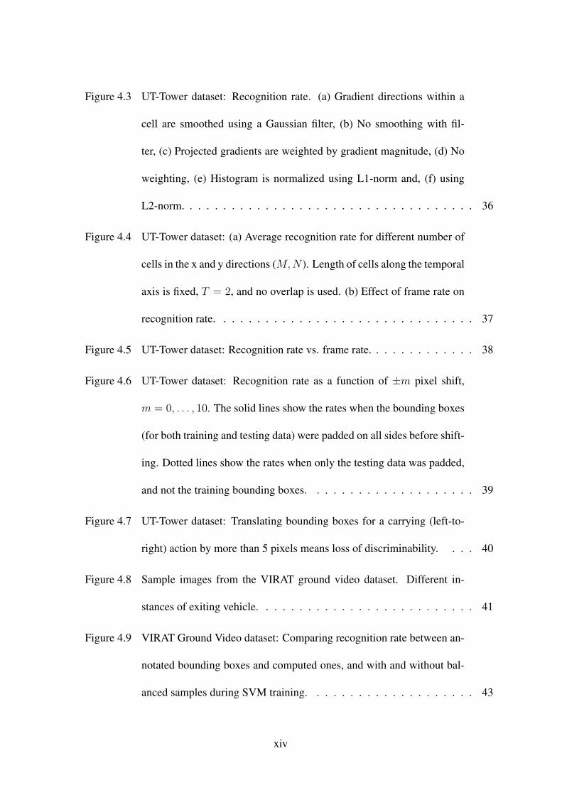
Figure 4.3 UT-Tower dataset: Recognition rate. (a) Gradient directions within a
cell are smoothed using a Gaussian filter, (b) No smoothing with fil-
ter, (c) Projected gradients are weighted by gradient magnitude, (d) No
weighting, (e) Histogram is normalized using L1-norm and, (f) using
L2-norm. . . . . . . . . . . . . . . . . . . . . . . . . . . . . . . . . . . 36
Figure 4.4 UT-Tower dataset: (a) Average recognition rate for different number of
cells in the x and y directions (M,N ). Length of cells along the temporal
axis is fixed, T = 2, and no overlap is used. (b) Effect of frame rate on
recognition rate. . . . . . . . . . . . . . . . . . . . . . . . . . . . . . . 37
Figure 4.5 UT-Tower dataset: Recognition rate vs. frame rate. . . . . . . . . . . . . 38
Figure 4.6 UT-Tower dataset: Recognition rate as a function of ±m pixel shift,
m = 0, . . . , 10. The solid lines show the rates when the bounding boxes
(for both training and testing data) were padded on all sides before shift-
ing. Dotted lines show the rates when only the testing data was padded,
and not the training bounding boxes. . . . . . . . . . . . . . . . . . . . 39
Figure 4.7 UT-Tower dataset: Translating bounding boxes for a carrying (left-to-
right) action by more than 5 pixels means loss of discriminability. . . . 40
Figure 4.8 Sample images from the VIRAT ground video dataset. Different in-
stances of exiting vehicle. . . . . . . . . . . . . . . . . . . . . . . . . . 41
Figure 4.9 VIRAT Ground Video dataset: Comparing recognition rate between an-
notated bounding boxes and computed ones, and with and without bal-
anced samples during SVM training. . . . . . . . . . . . . . . . . . . . 43
xiv

Figure 4.10 Sample images from VIRAT Aerial Video Dataset . . . . . . . . . . . . 44
Figure 5.1 The effect of increasing the number of actions on the UCF YouTube
Action dataset’s 11 actions by adding new actions from UCF50 using
only the motion descriptor. Standard Deviation (SD) and Mean are also
shown next to the action name. . . . . . . . . . . . . . . . . . . . . . . 54
Figure 5.2 Moving and stationary pixels obtained using optical flow. . . . . . . . . 55
Figure 5.3 Key frame selection from a given video. . . . . . . . . . . . . . . . . . 58
Figure 5.4 Performance of scene context descriptor on different number of key
frames. . . . . . . . . . . . . . . . . . . . . . . . . . . . . . . . . . . . 58
Figure 5.5 Effect of increasing the number of actions on the UCF YouTube Action
dataset’s 11 actions by adding new actions from UCF50, using only the
scene context descriptor. Standard Deviation (SD) and Mean are shown
next to the action name. . . . . . . . . . . . . . . . . . . . . . . . . . . 59
Figure 5.6 Performance of different methods to fuse scene context and motion de-
scriptors on UCF50 dataset. . . . . . . . . . . . . . . . . . . . . . . . . 61
Figure 5.7 Proposed approach. . . . . . . . . . . . . . . . . . . . . . . . . . . . . 63
Figure 5.8 Confusion table for UCF11 dataset using our approach. . . . . . . . . . 66
Figure 5.9 Confusion table for UCF50 using our approach. . . . . . . . . . . . . . 67
Figure 5.10 Performance as new actions are added to UCF YouTube (UCF11) Dataset
from the UCF50 dataset. . . . . . . . . . . . . . . . . . . . . . . . . . . 71
xv

Figure 6.1 The framework of action recognition using feature-tree. . . . . . . . . . 76
Figure 6.2 Tree structure defined by the intersection of bounding spheres and bound-
ing rectangles. . . . . . . . . . . . . . . . . . . . . . . . . . . . . . . . 77
Figure 6.3 Some examples of KTH dataset actions. . . . . . . . . . . . . . . . . . 82
Figure 6.4 Confusion table on KTH data set for 5 persons used in Random Forest. . 83
Figure 6.5 Confusion table on KTH data set for 5 persons used to grow feature-tree. 84
Figure 6.6 Performance comparison of using feature-tree on spatiotemporal fea-
tures. The number of features is increased from 10 to 200 and the near-
est neighbor search is increased from 1 to 50. . . . . . . . . . . . . . . . 86
Figure 6.7 Plot shows the effect on recognition performance with incremental ex-
amples from the new category added into the feature-tree. . . . . . . . . 88
Figure 6.8 Classification and localization of two actions happen in the same video.
The red features are classified into boxing, and blue is walking. . . . . . 89
Figure 6.9 Performance by increasing the number of frames considered in voting. . 90
Figure 6.10 Performance by increasing the number of frames considered in voting. . 92
xvi

LIST OF TABLES
Table 3.1 5 fold cross-validation on KTH dataset using different low-level video
representations . . . . . . . . . . . . . . . . . . . . . . . . . . . . . . . 27
Table 3.2 The performance on KTH by different bag of visual words approaches. . 27
Table 4.1 VIRAT Ground Video Dataset: Number of event-level annotated bound-
ing boxes and object-level boxes for training and testing. The numbers
in parentheses are the number of 3D spatiotemporal volumes extracted. . 42
Table 4.2 VIRAT Aerial Video dataset: Confusion matrix in recognizing station-
ary and moving actions. . . . . . . . . . . . . . . . . . . . . . . . . . . 45
Table 4.3 Performance comparison between 3D-STHOG and 3D-STHOPFF in
KTH, Weizmann and IXMAS datasets . . . . . . . . . . . . . . . . . . 47
Table 5.1 Action Datasets . . . . . . . . . . . . . . . . . . . . . . . . . . . . . . 50
Table 5.2 Performance of different motion descriptors on the KTH Dataset . . . . 52
Table 5.3 Performance comparison on KTH dataset . . . . . . . . . . . . . . . . . 70
Table 6.1 Nearest Neighbor Search. . . . . . . . . . . . . . . . . . . . . . . . . . 81
Table 6.2 Main steps of Action recognition using feature-tree. . . . . . . . . . . . 81
Table 6.3 The performance of the different bag of visual words approaches. . . . . 85
xvii

CHAPTER 1: INTRODUCTION
Vision is one of the most important senses used by humans to comprehend information
from the environment. Computer vision is a field developed to duplicate the human vision’s
ability to automatically understand the surroundings using cameras. Over the past few decades,
action recognition has been a very active research topic in computer vision. With over 35
hours of video uploaded every minute on YouTube, and thousands of surveillance cameras
on the ground and in the air, the need for reliable, automatic, and real-time computer vision
algorithms to do human/vehicle detection, tracking, action recognition, video retrieval, and
crowd monitoring has never been more important than it is now. In recent years, action and
gesture recognition has been used for human-computer interaction in console video games.
In this thesis, the focus is on effectively representing motion and static information in
videos, while simultaneously facilitating real-time incremental action recognition. The pro-
posed representation of video will produce a better representation of motion in videos for re-
liable feature representation. The importance of scene and context in action recognition is
explored, and an effective way to represent this static information is proposed. This thesis also
proposes a framework, based on local features and tree data structures, for indexing to achieve
real-time incremental action recognition.
1

1.1 Overview and Motivation
Video-sharing websites like YouTube consists of millions of movie clips, broadcast
videos, and amateur videos generated by users using their hand-held cameras or cell phone
cameras. Amateur videos are particularly noisy, low quality, and have poor lighting conditions
compared to movie or broadcast clips. Detecting a specific action or event in an amateur
video is of significant interest to government agencies, to identify suspicious activities. This
task can be challenging, and demands a reliable representation of video, feature detection and
extraction, and a robust classification or retrieval algorithm. Video surveillance from building
rooftops and airborne vehicles plays a major role in the war against crime, both domestically
and internationally. Public video surveillance is frequently being used as a traffic safety tool.
All these tasks require reliable detection, tracking, and action or event recognition algorithms.
In the case of aerial surveillance, the challenges are enormous due to the moving camera, low
resolution, and occlusion. Gesture and action recognition algorithms are increasingly being
used for human-computer interaction in both medicine to save lives, and console video games
to entertain people.
Accurate human action recognition has wide array of applications ranging from surveil-
lance to video games. In general, the goal is to automatically recognize the action performed
by one or more persons, given a sequence of images. A broad arrays of solutions have been
proposed over the past 20 years to solve this problem. The key to accurate action recognition
is the video representation used to generate the feature, and secondly the feature representation
itself. In recent years, significant attention has been given to motion based feature approaches,
which are considered to be most relevant for action recognition [8].
2

Research in image processing has shown that images can be represented using the pixel
intensity or the gradients. David Lowe [39] proposed one of the best feature representation
methods called Scale-Invariant Feature Transform (SIFT), which is based on image gradients.
Video can also be represented using the raw pixel intensity, spatial gradients, or optical flow
between consecutive frames. Pixel intensity values, spatial (2D) and temporal (3D) gradients
have been successfully used, but it is obvious to use optical flow to generate a feature descriptor
that represents motion in the video. Similar to the SIFT descriptor for images, PCA-Cuboids
(Intensities, gradients or optical flow) [12], 3DSIFT [51], 3DHOG [27], HOG, and HOF [30]
have been proposed for videos based on pixel intensities, gradients, and optical flow. We
believe that a better and powerful representation of video to do feature representation is needed
to understand the motion in videos and also, it is equally important to understand the scene and
context in the video.
Furthermore, the initial action recognition datasets captured in a controlled environment
lacked the realistic scenarios like scale variation, view point variation, multiple actors in the
scene, moving camera, noise, and low frame rate. Datasets such as KTH, Weizmann, and
IXMAS fall in this category called clean datasets. These so-called clean datasets have given
rise to approaches that assume human detection by background subtraction, tracking joints, 3D
representation of actions, human centric bounding boxes, and template based methods.
In recent years, challenging action recognition datasets have been released. The level of
complexity in the datasets has increased on many fronts for example, the number of categories,
categories with subtle differences, number of videos in dataset, and the camera motion in the
videos. UCF11, UCF-Sports, Hollywood dataset, UCF50, and VIRAT (Rooftop) datasets are a
3

few realistic datasets released to the community in the last few years. Most of the approaches
developed on clean datasets are practically not possible to apply to these new datasets, or if
applied would not perform as expected.
1.2 Contributions
In this thesis, we work on the most basic aspect of the action recognition task i.e., a
robust representation of the motion in videos in order to extract reliable motion features and
do action recognition in web videos, aerial and ground surveillance videos. We demonstrate
the importance of using static information in action recognition by introducing a scene-context
descriptor. We also propose the use of data structures at the local interest point level descriptors
to perform incremental action recognition. This work is a step towards a unified solution to
perform action recognition in environments with dynamic background and moving cameras,
and to address the incremental action recognition problem. Our major contributions in this
thesis are as follows:
• Using Particle Flow Field (PFF) as a low-level representation of video, which has better
performance than optical flow or gradients.
• Using 3D-Spatio Temporal Volumes (3D-STV) on the entire human bounding box, and
using a histogram of oriented 3D-Gradients and Particle Flow Fields to represent an
action.
• Understanding the scene and context in key frames, and using it in conjunction with the
motion descriptors.
4

• Developing a framework to do incremental action recognition using data structures based
indexing on local interest point descriptors.
• Creating a huge dataset of actions to understand the challenges of large and complex
datasets, and address problem, partially, by probabilistic fusion of motion and scene
context descriptors.
1.2.1 Particle Flow Fields to represent videos
Videos can be represented using raw pixel values, gradients, or optical flow. In this
work, we propose a better low-level representation of the video “Particle Flow Field” (PFF)
which is based on optical flow and particle advection. Optical flow at each pixel gives the
information of where that pixel moved in the next frame. This representation basically consists
of the motion information of each pixel between two consecutive frames. In order to have better
understanding of how a pixel moves and evolves, we do particle advection where each pixel in
a given frame is considered as a particle and we comprehend the motion of the particle over a
time period. Unlike optical flow which shows the velocity of a particle in two frames, particle
flow field captures the velocity of the same particle in n consecutive frames. Particle Flow Field
implicitly has the information to generate particle trajectories. Our low-level representation
PFF is novel in the following ways:
• “Particle Flow Field” is a more robust representation of motion in videos than optical
flow.
5

• PFF can be substituted in any action recognition framework where gradients and optical
flow are used.
• Motion descriptors generated using PFF have better performance than other low-level
representations such as gradients and optical flow in Bag of Visual Words framework.
1.2.2 3D - Spatio Temporal Volumes
3D-Spatio temporal volumes (3D-STV) are obtained by stacking the bounding boxes
of the detected human. The generated 3D-STV should be figure-centric, which demands good
human detection and tracking. In this work, we propose using 3D-Gradients and PFF in a spatio
temporal volume as low-level representation of the video. The underlying idea is an extension
of 3D-Gradients [27] used at the interest point level in a Bag of Visual Words framework. Our
work has the following contributions:
• Robust representation of motion in spatio temporal volumes using 3D-Gradients and
PFF.
• Motion descriptors generated using PFF have better performance than 3D-Gradients in
3D-Spatio temporal volume framework.
• Detailed set of experiments are done to understand the sensitivity of the proposed ap-
proach to scale, frame rate, and translation.
• Experimental results on six datasets: UT-Tower, VIRAT ground and aerial, IXMAS,
KTH, and Weizmann datasets.
6

• Unlike 3D-Gradients, PFF does not require tracking of a human to generate figure-centric
bounding boxes.
1.2.3 Scene context in web videos
Detection and tracking of humans is a challenging problem in itself. Instead of per-
forming human detection and tracking, we propose separating moving and stationary pixels
using optical flow, and introducing the notion of scene and context. In this work, we study the
effect of large datasets on performance, and propose a Bag of Visual Word framework that can
address issues with real life action recognition datasets (UCF50). The main contributions of
this work are the following:
• Provide an insight into the challenges of large and complex datasets, such as UCF50.
• We propose the use of moving and stationary pixels information, obtained from optical
flow, to generate a scene context descriptor.
• We show that as the number of actions to be categorized increases, the scene context
plays a more important role in action classification.
• We propose the idea of early fusion schema for descriptors obtained, which were ob-
tained from moving and stationary pixels, to understand the scene context, and finally
perform a probabilistic fusion of scene context descriptor and motion descriptor.
To the best of our knowledge, no one has attempted action/activity recognition on such
a large scale dataset (50 action categories) consisting of videos taken from the web (uncon-
strained videos) using only visual information.
7

1.2.4 Incremental Action Recognition Using Feature-Trees
The bag of visual words approach has been successfully used in the field of computer
vision. However, the majority of issues with the bag of visual words model are caused by
training-based quantization (visual vocabulary construction). In this chapter, we propose a
feature-tree structure to avoid training-based quantization. Our proposed method has many
advantages compared to the vocabulary-based action recognition approaches:
• First, we can effectively and efficiently integrate indexing and recognition using our pro-
posed feature-tree. As a result, we successfully avoid any intensive training (vocabulary
construction and category model training).
• Second, the feature-tree grows when additional training features are added from the new
training examples or new categories, making it very useful for incremental action recog-
nition in a variety of realistic applications.
• Third, it provides a disk-based data structure, which makes our recognition system scal-
able for a large scale dataset.
• Finally, the recognition is faster than real time. For example, for the KTH dataset, each
feature query takes 0.02s, and if each frame has approximately 3 features, it only takes
0.06s for the frame-based recognition, and the performance is still competitive. Ob-
viously, our system can also be used to detect multiple actions which are happening
simultaneously and localize them.
8

1.2.5 Challenging Datasets
One of the goals of this thesis is to propose methods that can be utilized in real world
applications. In order to achieve this, we have collected and released highly complex and huge
datasets, and performed extensive experiment using the approaches proposed in this thesis.
• UCF50: This dataset is an extension of the UCF YouTube dataset (UCF11). The ex-
tended dataset has a total of 50 action categories taken from YouTube, totaling to 6676
videos. The dataset is challenging in the following regards:
– Huge number of videos and 50 action categories
– Moving camera
– Not focused on the region of interest
– Poor quality of video, presence of compression artifacts, and low frame rate
• UCF-ARG: UCF - Aerial Rooftop Ground dataset is a multi-view human action dataset.
10 different actions performed by 12 actors were recorded from a ground camera, a
rooftop camera at a height of 100 feet, and an aerial camera mounted to a helium balloon.
The UCF-ARG dataset was not used in this thesis. The aerial view has the following
challenges:
– Low resolution, Scale variation, and View variations
– Top view has the problem of self-occlusion
– Few pixels on human or region of interest
9

1.3 Organization of the Thesis
The rest of the thesis is organized as follows. Chapter 2 summarizes the different ap-
proaches in action recognition by reviewing the existing literature. Chapter 3 introduces the
proposed new low-level video representation “Particle Flow Field” (PFF). In Chapter 4, 3D-
Gradients and the proposed PFF are used in 3D-Spatio Temporal Volumes, obtained using hu-
man detection and tracking. Chapter 5 proposes the use of scene context information obtained
by background and foreground separation, in conjunction with motion information to improve
action recognition in web videos. Chapter 6 presents the feature-tree framework to perform
incremental action recognition using SR-Trees. Finally, Chapter 7 concludes the thesis with a
summary of contributions and the possible future work.
10

CHAPTER 2: LITERATURE REVIEW
Over the past two decades, a wide variety of approaches have been used to solve the
problem of action recognition. Recent surveys provide a detailed description of the literature
in action recognition [57], [47]. In [47], the approaches were broadly classified as global and
local methods.
Global Representation: Global representation is obtained by detecting and tracking
the person, then stacking the sequence of the obtained region of interest (ROI) into a 3D spa-
tio temporal volume. 3D shape context [17], a combination of silhouettes and flow [26], 3D
shape flow over time [23], differential geometric properties [73] of the volume, and MACH
filter [49] have all been used to represent the 3D spatio temporal volume. Global methods have
shown good performance when the objects are localized and clearly visible. However, occlu-
sion or temporal variation is not handled effectively. Though temporal state-space models seem
promising on certain actions, they have limited generalizability. Moreover, the performance is
sensitive to model characteristics, such as order and state-specific distributions. Therefore
state-space models are not well suited for a general analysis of human action recognition per-
formance. Parts-based approaches are also not ideal because of the insufficient number of
pixels on the target.
Local Representation: Local representation typically involves detecting spatio tem-
poral interest points [29] [13] and representing a local region (2D or 3D or spatio temporal)
11

Figure 2.1: Figures 1(a) and 1(b) demonstrate 3D shape flow over time for a golf swing action
seen from two different views. Figure 2 shows the 3D action MACH filter synthesized from
the “Jumping Jack” action. Figure 3 shows the space-time template volume. Figure 4(a), 4(b),
and 4(c) represent the action volumes for action “walking” from three different views.(These
figures were taken from [23], [49], [26], and [73].)
around the interest point using a descriptor. In [29], 3D Harris corner points were detected
based on spatio temporal variations. The detected interest points are often not stable. The
stability issue was addressed in [13] by using Gaussian and Gabor filters in space and time,
respectively. Wang et al. [60] showed that dense sampling of interest points outperforms inter-
est point detectors. HOG ([10], [30]), HOF [30], 3DSIFT [52], eSURF [65], and HOG3D [27]
have been successfully used in a bag of feature framework. In HOG3D [27], 3D spatio tempo-
ral gradient orientations are quantized using regular polyhedrons. It was shown to outperform
HOG and HOF in the Hollywood and KTH datasets. The bag of feature framework lacks the
12

Figure 2.2: Bag of video words framework (local representation)
temporal aspect and fails to distinguish between dual actions, such as loading and unloading,
opening and closing, and getting in and out of vehicles, which involve similar types of motion
but in reverse temporal order.
2.1 Low-Level Representation of Video
Standard action recognition approaches propose a higher level of interpretation as men-
tioned above based on different low-level representations of videos. Good low-level video
representation help to design algorithms that disregard irrelevant information like the back-
13

ground, color of the clothes, and variation in illumination and are robust to variations in scale,
view-point and subtle variations in actions.
A video is a sequence of images, and the temporal information from those images is
important in defining an action. The raw information from the video is the pixel color or in-
tensity information. The spatio temporal variation of this pixel information can help identify
the actions, but not necessarily understand the actions fully. The temporal aspect can be intro-
duced by taking a series of patches with intensities. However, the pixel information could be
redundant and is variant to color, lighting conditions, etc. As demonstrated by Johansson [22]
using moving light displays (MLDs), the static information remains meaningless compared to
the relative motion. Information related to the background, the color of the clothes, and il-
lumination conditions do not help in action recognition. The spatial gradients (2D-Gradients)
could make it invariant to color and illumination, and spatio temporal gradients (3D-Gradients)
can help bring the temporal aspect into consideration. Raw pixel intensities and gradients have
been successfully used in tasks related to single image and videos. Since the task of action
recognition is based on a sequence of frames and understanding the different motion patterns
in the video [12] [31] [10] [27], the optical flow computed between consecutive frames has
proven to be a good low-level representation of video [12] [31]. Silhouettes [26] and 3D vol-
ume shapes [17] have also been used to represent the videos for action recognition, which
require good foreground and background segmentation.
14

2.2 Action Recognition in Large Realistic Datasets
Categorizing a huge number of classes has been a bottleneck for many approaches
in image classification/action recognition. Deng et al. [11] demonstrated the challenges of
performing image classification on 10,000 categories. Recently, Song et al. [55] and Zhao et
al. [62] attempted to categorize a huge numbers of video categories using text, speech, and
static and motion features. Song et al. [55] used visual features, such as color histograms, edge
features, face features, SIFT, and motion features, and showed that text and audio features
outperform visual features by a huge margin.
Template based methods [5], modeling the dynamics of human motion using finite state
models [20] or hidden Markov models [66], and Bag of Features models [36, 12, 37, 68] (BOF)
are a few well known approaches taken to solve action recognition. Most of the recent work
has been focused on BOF in one form or another. However, most of this work is limited to
small and unconstrained datasets.
Extracting reliable features from unconstrained web videos has been a challenge. Ac-
tion recognition in realistic videos was addressed recently by Laptev et al. [32] and Liu et
al. [36, 37]. Liu et al. [36] proposed pruning the static features using PageRank and motion
features using motion statistics. Fusion of these pruned features produced a significant increase
in the performance on the UCF11 dataset. Ikizler et al. [21] used multiple features from the
scene, object, and person, and combined them using a Multiple MIL (multiple instance learn-
ing) approach. Fusion of multiple features extracted from the same video has gained significant
15

interest in recent years. A study by Snoek et al. [58] does a comparison of early and late fusion
of descriptors.
There has been no action recognition work done on huge datasets using only visual
features. In this thesis we propose a framework which can handle these challenges.
2.3 Action Recognition using Tree Data Structures
Action recognition using bag of visual words has been widely explored recently, and
very impressive results have been reported on the public KTH dataset [12] [37] [30] [33] [68].
However, to the best of our knowledge, the use of tree data structures to integrate indexing,
recognition, and localization has not been explored for action recognition.
Tree data structure has been widely used in visual recognition. For instance, kd-tree [3]
has been used for fast image matching [39] [2]. However, it might reconstruct the entire tree if
it is seriously unbalanced, due to dynamic update [25]. Therefore, it is not scalable and unable
to handle a large scale feature dataset efficiently. Vocabulary-based methods (bag of visual
words) are proposed to reduce the number of features by quantization, for compact visual rep-
resentation [14] [12] [37] [53] [45] [33] [67]. Recently, varied tree-based approaches have been
proposed to construct vocabulary trees. Nister et al. [45] used hierarchical k-means to quickly
compute very large vocabularies. Random Forest models have been successfully utilized for
recognition. Instead of using Random Forest as a classifier, Moosmann et al. [43] used similar
techniques to construct random vocabulary trees in a supervised mode. This obtained signifi-
cantly better performance than the unsupervised vocabulary construction approaches, such as
k-means. Since most vocabulary construction methods are training-based, they are unable to
16

Baseball Pitch Basketball Shooting BikingBench Press Billiards
Breaststroke Clean and Jerk DrummingDiving Fencing
Golf Swing High Jump Horse RidingHorse Race Hula Hoop
Javelin Throw Juggling Balls Jump RopeJumping Jack Kayaking
Lunges Military Parade Nun chucksMixing Batter Pizza Tossing
Playing Guitar Playing Piano Playing ViolinPlaying Tabla Pole Vault
Pommel Horse Pull Ups Push UpsPunch Rock Climbing Indoor
Rope Climbing Rowing Skate BoardingSalsa Spins Skiing
Ski jet Soccer Juggling TaiChiSwing Tennis Swing
ThrowDiscus Trampoline Jumping Walking with a dogVolleyball Spiking Yo Yo
Figure 2.3: Screenshots from videos in the UCF50 dataset, showing the diverse action cate-
gories.
17

update the vocabulary dynamically. This significantly limits their applications in the real world.
In order to overcome this, Yeh et al. [71] proposed a forest-based method to create adaptive
vocabularies, which can update the vocabulary without reconstructing the entire tree. It is ef-
ficient for image retrieval; however, it still requires re-training the category models for recog-
nition when the vocabulary has been updated using the new training examples or categories,
because the image representations have been changed with the update of the vocabulary.
Using trees to index the bag of features and then perform recognition on it, has not
been addressed extensively. Randomized trees have been used in [34] and [42] for image view
recognition. They used simple binary trees and split a node by checking the entropy of point
labels. Boiman et al. [6] also used kd-tree for fast feature search in their image classification.
However, used only simple trees, which do not support efficient dynamic update. They are not
suitable for large scale datasets or applications with dynamic environments.
Little work has been done in the action recognition area using trees to index bag of
spatiotemporal features. Instead of detecting spatiotemporal interest points, Mikolajczyk et
al. [42] detected local static features from each frame, then trained the vocabulary forest by hi-
erarchical k-means. They obtained good results on the KTH dataset. However, their approach
also faces the problem of dynamic update of vocabulary, so it is unable to cope with incre-
mental action recognition for most real applications. Besides, their system is not real time.
In this thesis, we propose the use of feature-trees to address issues such as incremental action
recognition and frame-by-frame action recognition, and develop a real-time action recognition
system.
18

CHAPTER 3: PARTICLE FLOW FIELD
3.1 Introduction
Extensive research has been done on designing robust motion descriptors for action
recognition in the computer vision field. Action recognition approaches can be broadly cat-
egorized into global and local representations, as discussed in Chapter 2. Irrespective of the
approach or the framework, different video representations [12] [72] [59] [57] like raw pixel
values, gradients, optical flow, 2D shape/contours, Silhouettes, and 3D volume shapes, have
been used as the building block for descriptor generation. Some video representations are in-
variant to illumination, a person’s clothing, scale, and view point and others simply consider
edges or the motion at pixel level. Each video representation has its own advantages, draw-
backs, and challenges. For instance, the optical flow computed is usually noisy, silhouettes and
2D shape need good segmentation and background subtraction, and 3D volumes need complex
pre-processing steps.
In this chapter, a robust video representation “Particle Flow Field” (PFF) is proposed,
which is based on optical flow and particle advection. Experimental results on KTH dataset
using the Bag of Video Words (BoVW) framework show that the proposed particle flow field
outperforms video representations like spatial gradients (2D-Gradients), spatio temporal gra-
dients (3D-Gradients), and optical flow.
19

3.2 Low-Level Video Representation
A video is a sequence of still images through which the motion in the scene is rep-
resented. This spatio-temporal variation in pixel intensity is a massive amount of raw infor-
mation, which does not necessarily help understand and recognize the action/activity in the
video. Johansson [22] showed in his classic experiment that humans can understand the action
by seeing only point light sources placed at a few limb joints with no additional information.
Over the past few decades, many different ideas have been proposed to achieve a robust video
representation on which reliable action recognition systems can be developed. In this section
we describe a few low-level representations, and propose a new representation.
3.2.1 Normalized Pixel Values
In videos, the intensity at each pixel varies spatially and temporally. The variation in
this raw intensity information at every pixel is shown in Figure 3.1(a), which can help one
better understand the video. Dollar et al. [12] used normalized pixel values, but reported low
performance compared to other video representations like gradient and optical flow. The reason
is clearly that most of the intensity information, such as background and color of the clothes,
is not relevant to the task of understanding and identifying the action performed in the video.
3.2.2 Gradients
Gradients have been used as robust image and video representation [12] [31] [10] [27].
Each pixel in the gradient image helps extract relevant information, e.g. edges, to do reliable
action recognition. Gradients can be computed at every spatio-temporal location (x, y, t) in any
20

Figure 3.1: Different video representations.21

direction in a video. In general, gradients (Gx, Gy, Gt) are extracted in horizontal, vertical, and
temporal directions, respectively, by convolving the images with a filter to obtain approximate
derivatives. Sobel filter for horizontal and vertical gradients are as shown:
Gx =
−1 0 +1
−2 0 +2
−1 0 +1
∗ A and Gy =
−1 −2 −1
0 0 0
+1 +2 +1
∗ A,
where A is an image and ∗ denotes convolution operation. Figure 3.1(b,c) shows the spatial
gradients commonly referred to as 2D-Gradients, where as Figure 3.1(b,c,d) depicts the spatio-
temporal gradients referred to as 3D-Gradients. The orientation and magnitude of (Gx, Gy, Gt)
have been successfully used by [31] and [27] for action recognition.
3.2.3 Optical Flow
Optical flow describes the approximate motion of each pixel between two consecutive
frames. In a broader sense, one can obtain apparent motion (velocity) of regions or moving
objects in a video. Since actions are defined by the motion of body parts, optical flow tends to
be a better low-level representation of a video, to build a reliable motion descriptor. The optical
flow between two consecutive frames f1 and f2 is represented by V = (u, v), where u and v
are the horizontal and vertical components of optical flow. Optical flow at a pixel location
(x, y) can be represented as V (x, y) = (u(x, y), v(x, y)). Given a sequence of n frames S =
f1, f2, . . . , fn from a video, the collection of optical flows from all consecutive frames in S
can be defined as a time-dependent optical flow field V (t), where t = 1, 2, . . . , n − 1. The
Lucas-Kanade optical flow algorithm [40] has typically been used to compute the optical flow
22

between consecutive frames. The recently proposed optical flow algorithm by Lui et al., [35]
provides better optical flow than Lucas-Kanade [40], but is slow. Figure 3.1(d) shows a sample
color coded optical flow, obtained using the code provided by [35]. Optical flow has been
successfully used by [12] and [31] for action recognition, however the majority of optical flow
algorithms are not accurate, and their accuracy depends on the parameters.
3.2.4 Particle Flow (Particle Velocity)
For a given sequence of n frames S = f1, f2, . . . , fn, a grid of particles is placed
on the first frame f1 and moved across all the n frames using the optical flow field V (t). The
process of moving the particles using time-dependent optical flow fields O(t) (3D volumes of
optical flow fields) is called particle advection, which results in Particle Trajectories [1], also
known as Pathlines, as depicted in Figure 3.1(f). Let (xi(t), yi(t)) be a particle position at time
t, where t = 1, 2 . . . , n, i = 1, 2 . . . , N , and N is the number of particles. Particle advection is
performed to estimate the location of the particle i at time (t + 1) by interpolating the optical
flow at the sub-pixel level. As performed in [1], the new location (xi(t + 1), yi(t + 1)) is
estimated by numerically solving the following equations:
xi(t+ 1) = xi(t) + u(xi(t), yi(t)), (3.1)
yi(t+ 1) = yi(t) + v(xi(t), yi(t)) (3.2)
The optical flow or velocity along a particle’s path (trajectory) is called Particle Flow
or Particle Velocity, which is shown in Figure 3.1(e). The trajectory of a particle i from frames
t = 1, 2 . . . , n is represented as:
(3.3)ti = [xi(1), yi(1)], [xi(2), yi(2)], . . . , [xi(n− 1), yi(n− 1))],
23

and similarly, the particle flow of a particle i from frames t = 1, 2 . . . , n is represented as:
(3.4)pi = [u(xi(1), yi(1)), v(xi(1), yi(1))], [u(xi(2), yi(2)), v(xi(2), yi(2))],. . . , [u(xi(n− 1), yi(n− 1)), v(xi(n− 1), yi(n− 1))],
where u(xi(t), yi(t)) and v(xi(t), yi(t)) are the horizontal and vertical components of optical
flow of the ith particle at location (xi(t), yi(t)) and t = 1, 2, . . . , n − 1. Particle Flow Field
(PFF) for a time period of T starting at time t is represented by:
P t+Tt = p1, p2, . . . , pN, (3.5)
and Particle Flow Map (PFM) is represented by:
T t+Tt = t1, t2, . . . , tN, (3.6)
where N is the number of particles initiated at time t and tracked till time (t+ T ).
Particle Flow Maps and Particle Trajectories have been used to do scene flow segmen-
tation in videos ( [1] and [41]). In order to understand the background dynamics, one has to
constantly initiate particles at the same location and understand their behavior with respect to
time, which was studied by Mehran et al. and calls them streaklines. According to [41], streak-
lines represent the locations of all particles at a given time that passed through a particular
point.
In action recognition, the focus is on the foreground and particle flow is more appro-
priate compared to streaklines [41] and Particle Flow Maps [1]. As described earlier, particle
flow is being used to study the velocity at which the particles move over time. This informa-
tion is implicitly available in particle trajectories which were used by [70]. In [70], chaotic
24

invariant features are extracted to generate the motion descriptor. The derivative of the particle
trajectories gives the velocity of the particle at different times, which is particle flow (particle
velocity). Likewise, particle trajectories can be obtained using Particle Flow Fields, i.e. the
evolution of particles over time.
3.3 Experiments
In order to evaluate the performance of different low-level video representations, we
performed experiments on the KTH dataset. The KTH dataset has 6 actions categories, per-
formed 4 times by 25 actors. Motion descriptors are extracted from the interest points, which
were detected using Dollar’s detector [12]. At every interest point location (x, y, t) , we ex-
tract a 3D cuboid of dimension W × H × T , where W and H are the width and height of
the patch, respectively, and T is the number of patches. 3D-Cuboid is a collection of patches
with (x, y, t) as the center point. The extracted 3D-Cuboid is represented using the following
low-level representations:
2D-Gradient: At any given interest point location in a video (x, y, t), a 3D cuboid is
extracted. The brightness gradient is computed in the horizontal and vertical direction in this
3D cuboid, which gives rise to 2 channels (Gx, Gy).
3D-Gradient: The gradient along temporal direction is also considered in the extracted
3D cuboid, which gives rise to 3 channels (Gx, Gy, Gt).
Optical Flow: The Lucas-Kanade optical flow [40] is computed between consecutive
frames in the 3D cuboid centered at (x, y, t) to obtain 2 channels (Vx, Vy).
25

Particle Flow Field: A dense grid of particles is initiated in the first patch of the
extracted 3D cuboid. The computed Lucas-Kanade optical flow is used to advect the particles
to generate the 2 channels (Px, Py) of the particle flow field.
The obtained channels in each representation are flattened into a vector, and PCA is
applied to reduce the dimension. All of the above descriptors are extracted from the same
location of the video and the experimental setup is identical. We use BOF paradigm and SVM
to evaluate the performance of each descriptor.
Bag of Video Words (BoVW) Framework: Interest points are detected from every
training video using Dollar’s detector [12]. At each of these interest points, a 3D-Cuboid is
extracted and is represented using different low-level representations. The channels obtained
from each representation are flattened into a long vector, as explained above, which leads to a
high dimension descriptor. PCA is used to reduce the dimension of the descriptors. These low
dimension descriptors are clustered into K clusters using k-means. The center of each cluster
represents a codeword in a codebook of size K. All the motion descriptors are quantized using
the nearest codeword. The histogram of the quantized descriptors in a given video represents
a Bag of Visual Words (BoVW) descriptor. SVM classifier is trained on the BoVW descriptor
from all of the training videos.
In the experiments on the KTH dataset, we do 5 fold cross-validations. In each valida-
tion, we train on videos from 10 actors and test on the remaining 15 actors. Table 3.1 shows
the performance of all the video representations in the BoVW framework. It can be observed
that the proposed Particle Flow Field performed the best and 3D-Gradients followed behind.
26

Table 3.1: 5 fold cross-validation on KTH dataset using different low-level video representa-
tions
10 Training Videos Bag of Video Words Framework (Dollar detector)
Codebook Size 200 500 1000 2000 5000
Gradient (Gx, Gy, Gt) (3D-Gradients) 84.39% 86.62% 88.30% 88.74% 89.35%
Gradient (Gx, Gy) (2D-Gradients) 86.40% 86.85% 88.13% 88.24% 88.96%
Optical Flow 84.90% 88.69% 87.40% 88.02% 88.69%
Particle Flow Field (HOPE) 86.78% 89.79% 88.96% 91.30% 91.15%
Table 3.2: The performance on KTH by different bag of visual words approaches.
Method Acc(%) Method Acc (%)
Particle Flow Field 93.0 Neibles, et al. [44] 81.5
Liu, et al. [38] 91.3 Dollar, et al. [13] 80.6
Wong, et al. [69] 83.9 Schuldt, et al. [50] 71.7
Leave-one-actor-out cross-validation in the BoVW framework using the Dollar detector
is performed to compare with the state-of-the-art results. Particle Flow Field performed 93.00%
compared to 91.30% using 3D-Gradients. Table 3.2 compares the performance of the proposed
approach with other state-of-the-art approaches.
3.4 Summary
In this chapter, we proposed a new low-level video representation “Particle Flow Field”,
which is based on optical flow and particle advection. We showed that particle flow field
27

performs better than other video representations, such as 2D-Gradients, 3D-Gradients, and
Optical Flow. The only drawback of using particle flow fields is that, it has to be computed over
optical flow by performing particle advection, which makes it slower than just using optical
flow as low-level video representation.
28

CHAPTER 4: 3D - SPATIO TEMPORAL VOLUMES
4.1 Introduction
Research in human action recognition continues to progress across a wide gamut of
actions ranging from simple actions like walking, running and jumping to more complex ones
such as interacting in a meeting room, loading a car, etc. [16], [46]. The latter are complex
in that they may be characterized as a sequence of simpler actions, and that they may involve
interactions with other objects. Early datasets like KTH and Weizmann have promoted signifi-
cant algorithmic advancement [57], [47] and may be deemed ’solved’ because most techniques
report near-perfect results. But the advancement is rarely reflected in performance over newer
datasets like the VIRAT dataset [46] that are challenging, and need approaches that are robust
and generalize well. The assumption of richness of data, near-perfect preprocessing in track-
ing and action localization does not necessarily hold over large, real-world datasets. Some
approaches are not affected by these problems, e.g., when registration and object tracking is
not be used, when the data is of high-resolution and without camera motion [30], and so on. In
surveillance however, these problems are inherent.
In this chapter, we analyze the state of the art in action recognition using histogram of
3D spatio temporal gradients (3D-STHOG)1. We choose the following six datasets for exper-
1We use ’3D-STHOG’ instead of 3DHOG to note that gradients are computed in a spatiotemporal volume,and not in 3D spatial coordinates.
29

iments: UT-Tower, VIRAT ground and aerial, IXMAS, KTH and Weizmann datasets. Exper-
imental analysis discussed in section 4.4 confirms certain commonly-held notions and shows
some surprising results:
• Recognition in UT-tower dataset seems to be robust to a limited range of scale variations
(∼15%), or reduction in frame rate (to about ∼6 fps ).
• It is best to use similar preprocessing during training and testing, i.e., it does not help to
train on pristine annotations and test with noisy tracker results.
• A small shift in bounding boxes can severely affect recognition – a 10% (2 px in UT
tower data) shift can produce a 20% reduction in average recognition rate.
• A moderate misalignment (bounding box shift of 4 pixels) can affect discriminability
drastically.
Thus we attempt to provide an analysis of data and popular algorithms which may
benefit future research in action recognition. We do not propose a novel technique in this work,
and use an existing, state-of-the-art technique with some slight modifications. Incidentally, the
factors mentioned here and their related aspects which limit generalizability have received an
enormous amount of attention in the object recognition community in recent years [56]. It
is perhaps premature to enter into a similar level of scrutiny in action recognition given that
the sub-field is relatively less mature. Nevertheless, we believe that such an analysis would
be beneficial at a time when more and more papers are addressing datasets beyond the simple
ones.
30

We also analyze the performance of histogram of oriented particle flow field (3D-
STHOPFF) in section 4.3 and compared the results to the state of the art 3D-STHOG on three
datasets: KTH, Weizmann and IXMAS datasets in section 4.5 and show that:
• 3D-STHOPFF outperforms 3D-STHOG is all the three datasets.
• 3D-STHOPFF does not need figure centric bounding boxes.
4.2 Histogram of Oriented 3D Spatiotemporal Gradients (3D-STHOG)
There are three main stages involved in computing the probability of actions given a
video. They are: detection and tracking, feature extraction, and classification. This stage
outputs a sequence of bounding boxes containing moving objects of interest which is input to
the feature computation stage before classifying using trained SVMs. We focus on 3D-STHOG
for analysis, and present comparative results with HOG and HOF in a bag of words framework.
Klaser et al. introduced a HOG descriptor based on 3D spatiotemporal gradients as a
generalization of HOG [10]. We follow the same procedure as described in [27] with a few
minor differences as described next (Figure 4.1).
Preprocessing: The sequence of bounding boxes computed by the tracker need not be
of constant size. To simplify gradient computation, we fix the spatial size of spatiotemporal
volume to be the size of the bounding box in the first frame of the volume. Thus several
spatiotemporal volumes are extracted for every track with a fixed overlap in time and space.
Gradients along x,y,t: For each spatiotemporal volume, gradients are computed along
x, y, t directions.We do not use multiple scales [27], instead use a fixed number of cells for
31

Figure 4.1: Computing the 3D-STHOG
the spatiotemporal volumes. Section 4.4.1.1 demonstrates the sensitivity of feature to scale
changes.
Gradient quantization and weighting: Gradient orientations are then quantized by
projecting the 3D vector on to a regular polyhedron. Empirically, we found that icosahedron
(20-sided) performed well. We have fixed this choice throughout the chapter. The projected
gradients are then weighted by the gradient magnitude at that pixel.
Histogram: The spatiotemporal volume is divided into a fixed number of cells, with
overlap along x, y, t axes. Results with various choices of number of cells are shown in sec-
tion 4.4. Within each cell (size M ×N × T ), a Gaussian filter is used to smooth the weighted
gradients. Their histogram is then computed using a fixed number of bins. The histograms of
32

Figure 4.2: Computing 3D-STHOPFF descriptor. Grid of particle are initiated at frame n and
red pathlines are obtained using forward optical flow and blue pathlines using backward optical
flow
all the cells in the spatiotemporal volume are concatenated and normalized using the L2 norm
to obtain the 3D-STHOG signature of the tracked object.
Classification using SVM: The histogram features are used to train an SVM classifier
with histogram intersection kernel. Experimentally, histogram intersection kernel performed
better than RBF kernel (95.37% vs. 90.74% in UT-Tower dataset). Leave-one-out procedure
was used.
33

4.3 Histogram of Oriented Particle Flow Fields (3D-STHOPFF)
The steps involved in 3D-STHOFF are explained as follows (Figure 4.2):
Preprocessing: In a given video, human detection on one frame is needed. 3D-
STHOFF does not need the bounding box to be tracked.
Particle Flow Fields: Grid of particles are placed in the detected human bounding box.
Forward and backward optical flow for the video are computed and used for particle advection.
The particles initiated at frame n are moved in forward direction till frame m using forward
optical flow computed between frame n and m. Similarly, the particles initiated at frame n are
moved in backward direction till the first frame using backward optical flow computed between
first frame and frame n. Since particle advection over large number of frames tends not to be
accurate, we do particle advection in forward shown in red in Figure 4.2 and backward direction
shown in blue in Figure 4.2 to get better particle flow fields. The velocities with which the grid
of particles move in both direction are captured in the particle flow field.
Quantization and weighting: Particle Flow Field has two components, horizontal and
vertical components. The orientation of the particle flow field is quantized into 20 bins and
weighted with their magnitude. 20 bins are selected to be consistent with 3D-STHOG for
comparison.
Histogram: The particle flow field volume is divided into overlapping cells similar
to 3D-STHOG. Gaussian filter is used to smooth the weighted gradients and the computed
histogram from all cells are concatenated and normalized using L2 norm.
34

Classification using SVM: Similar to 3D-STHOG, SVM classifier with histogram in-
tersection kernel is used.
4.4 Experiments using 3D-STHOG
We use six datasets for experiments as described below. KTH and Weizmann datasets
were chosen for historical reasons. IXMAS dataset is used to test sensitivity to viewing direc-
tion, in a controlled setting. Before applying the algorithms on the large-scale VIRAT ground
and aerial datasets, we conducted a series of experiments using UT-tower dataset to better un-
derstand the features. The viewing angle in this dataset is somewhat similar to those in aerial
video datasets, and it is less noisy.
4.4.1 UT-Tower Dataset
The UT-Tower dataset consists of nine human actions: pointing, standing, digging,
walking, carrying, running, waving (two types) and jumping performed by twelve actors.
Videos are captured by a stationary camera with 306 × 240 resolution and 10 fps. All the
videos belong to one of the above action classes. The average height of people is about 20
pixels. Spatiotemporal volumes are computed as described in sec. 4.2. Every volume is then
divided into M ×N × T cells, 3D-STHOG is computed and used to train SVMs.
Leave-one-out procedure is used for consistency with [9]. The best performance of
95.37% accuracy in recognition was obtained using 3× 3× 2 cells (Figure 4.3). Here gradient
projections were (a)smoothed within a cell, (b) weighted by their magnitude and (c) normal-
ized using L2−norm. In comparison, [9] obtained 100% recognition by pre-processing the data
35

Figure 4.3: UT-Tower dataset: Recognition rate. (a) Gradient directions within a cell are
smoothed using a Gaussian filter, (b) No smoothing with filter, (c) Projected gradients are
weighted by gradient magnitude, (d) No weighting, (e) Histogram is normalized using L1-norm
and, (f) using L2-norm.
– using shadow removal technique to detect shadow pixels and fill in the shadow pixels with
background. Then, tightly-centered bounding boxes were computed which improved recogni-
tion in their experiments. In our case the bounding boxes are comparable to the output of a
typical detection and tracking system. Figure 4.4(a) shows the performance when M,N are
varied with T = 2 and no overlap in x, y or t directions.
4.4.1.1 Sensitivity to Scale
Figure 4.4(b) shows the change in performance for various cases:
Case 1: Training and testing data is of the same resolution: The recognition rate is
more than 90% as long as the boxes are at least as big 0.60 times the original size (blue curve
36

Figure 4.4: UT-Tower dataset: (a) Average recognition rate for different number of cells in the
x and y directions (M,N ). Length of cells along the temporal axis is fixed, T = 2, and no
overlap is used. (b) Effect of frame rate on recognition rate.
in fig.Figure 4.4(b)). When the size of the boxes are less than 0.60 times the original bounding
box size, people are typically less than 12 pixels tall.
Case 2: Training data is 0.75 times of the original resolution, testing data resolution
is varied from 1 to 0.50 times the original resolution. In this case, the 90+% recognition rate
is maintained as long as the testing data size is at least ∼0.7 times the original resolution. (red
curve in fig.Figure 4.4(b)).
Case 3: Training data is of the original resolution, testing data resolution is varied
from 1 to 0.50 times the original resolution. This has worse performance than the previous
cases with 90+% recognition rate maintained as long as the testing data resolution is at least
∼0.82 times the original resolution (green curve in fig.Figure 4.4(b)).
Case 4: Training data is 0.5 times the original resolution, testing data resolution varies.
This does not perform well (purple curve in fig.Figure 4.4(b)).
37

Figure 4.5: UT-Tower dataset: Recognition rate vs. frame rate.
Thus 3D-STHOG is robust to variations in scale to about 15%, i.e., when training and
testing data resolutions are within 15% of each other, recognition is good.
4.4.1.2 Sensitivity to Frame Rate
Figure 4.5 shows the change in recognition rate with frame rate. The frame rate is
varied from 1 fps to 10 fps (original frame rate) by simply dropping frames in between. The
average performance (red dashed curve) generally improves with increase in frame rate except
for a dip in performance for 6 fps. The dip was caused in excessive confusion between the two
types of waving.
4.4.1.3 Sensitivity to Translation (Misalignment)
In this set of experiments (results in Figure 4.6), the bounding boxes were translated
(in x and/or y) directions to test the sensitivity of the features to noisy detection and tracking.
Surprisingly, even a shift of ±2 pixels can cause a reduction in recognition rate from ∼95%
38

Figure 4.6: UT-Tower dataset: Recognition rate as a function of±m pixel shift,m = 0, . . . , 10.
The solid lines show the rates when the bounding boxes (for both training and testing data) were
padded on all sides before shifting. Dotted lines show the rates when only the testing data was
padded, and not the training bounding boxes.
to ∼75%. To put this shift magnitude in context, recall that people are typically 20 pixels
tall in this dataset. So ±10% translation of the bounding boxes can cause a 20% reduction in
performance. We found that increasing the size of bounding boxes in all directions by a few
pixels can mitigate the drop in performance to a certain extent. Further, it is better to train
with noisy data instead of pristine data. If the training data is relatively noise-free, but the
testing data is corrupted by noise (i.e., above-mentioned translation of bounding boxes), then
the performance can be ∼10% poorer than when both training and testing data have similar
noise characteristics.
We conducted a simple experiment to find out the effect of bounding box translation
on discriminability of actions. Using carrying and walking left-to-right (L-R) in the image
39

Figure 4.7: UT-Tower dataset: Translating bounding boxes for a carrying (left-to-right) action
by more than 5 pixels means loss of discriminability.
as an example, we consider two other actions - carrying right-to-left (R-L) and pointing. We
shift the bounding boxes for these actions and compare the distance between their 3D-STHOG
signatures using histogram intersection. As long as the shift is less than 4 pixels (20% of 20
pixel tall person), the three samples are discriminable. Beyond this number, shifted version of
carrying L-R is about the same distance from its unshifted version as pointing or carrying R-L
so that the actions become indistinguishable.
4.4.2 VIRAT Ground Video Dataset
The VIRAT video dataset consists of ∼25 hours of video collected in eleven scenes,
∼7 hours of which are being released in batches. In this work, we used 2.75 hours for training
and remaining for testing from six scenes (3 for training, 3 unseen scenes for testing). The
dataset consists of 23 actions which includes single person actions and those involving interac-
tions with vehicles and facilities. We focus on six human-vehicle interaction actions - opening
the trunk, closing the trunk, loading a vehicle, unloading a vehicle, getting into and out of a
40

Figure 4.8: Sample images from the VIRAT ground video dataset. Different instances of
exiting vehicle.
vehicle.Two types of ground truth annotations are provided: event-level bounding boxes and
object-level bounding boxes. Event-level boxes include the spatiotemporal context around the
object of interest. For example, an event-level box for loading includes both the person load-
ing the vehicle and a large part of the vehicle, its object-level box only contains the person.
We have used both these types of boxes in experiments. Table 4.1 summarizes the number of
instances of actions in the two cases.
There are two main challenges in this dataset: the videos come from different scenes
which creates significant variability in viewing direction, style of actions and other conditions.
In these actions involving interactions with vehicles, people often tend to be occluded severely.
Consequently motion detection and tracking fails. For example, Figure 4.8 shows a cropped
region of three instances of exiting vehicle.
With Context (Annotated Event Bounding Boxes): First we conduct a series of ac-
tion recognition experiments using the annotated bounding boxes provided with the dataset.
Each spatiotemporal volume is classified into one of seven classes (six action classes and one
unknown class that includes background). Multiclass SVM was trained using the histogram
intersection kernel. The number of training and testing samples are specified in Table 4.1. The
41

Table 4.1: VIRAT Ground Video Dataset: Number of event-level annotated bounding boxes
and object-level boxes for training and testing. The numbers in parentheses are the number of
3D spatiotemporal volumes extracted.
Action # Train # Test # Train #Test
event event objects objects
Load 11 (35) 50 (187) 3 (28) 28 (95)
Unload 15 (53) 59 (279) 11 (54) 51 (236)
Open trunk 18 (48) 47 (123) 12 (38) 27 (73)
Close trunk 19 (41) 46 (104) 11 (31) 35 (74)
Get in veh. 61 (374) 115 (847) 35 (228) 69 (489)
Get out of veh. 63 (445) 92 (475) 40 (330) 40 (205)
Unknown 2 (24) 0 (0) 2 (46) 0 (0)
dataset is clearly unbalanced in that some classes have more than 60 samples, whereas others
have 10-15 samples. Our experiments show that balancing the training set, i.e., ensuring the
same number of training samples across most of the action classes, improves performance in
general. The results are summarized in Figure 4.9.
No Context (Annotated Object Bounding Boxes): A similar set of experiments was
then conducted with spatiotemporal volumes created by tracks that were computed using the
object-level bounding boxes. The results are summarized in Figure 4.9. Context seems to help
as the performance with event-level bounding boxes is better than that of object-level boxes.
Secondly, loading performed much worse in the experiment with computed bounding boxes,
whereas unloading did not show a similar degradation. Given that very few loading instances
42

Figure 4.9: VIRAT Ground Video dataset: Comparing recognition rate between annotated
bounding boxes and computed ones, and with and without balanced samples during SVM
training.
were detected after the tracking stage, it is difficult to ascertain reasons for low performance at
the action recognition stage.
Comparison with Interest-point Based Methods: Harris3D detector [29] is used to
detect Harris corner points to extract spatiotemporal interest points (STIP). HOG and HOF de-
scriptors [30] are then computed to characterize the 3D spatiotemporal video patch extracted at
each interest points. The 3D video patch is divided into 3× 3× 2 cells and 4-bin histogram of
gradient orientations (HOG) and 5-bin histogram of optical flow (HOF) are computed in each
cell and the normalized histograms of HOG (72 dimensions) and HOF (90 dimensions) are
concatenated. Then, the features are encoded in a Bag of Words framework. Codebooks of dif-
ferent sizes are generated using the HOG/HOF extracted from training videos. A histogram of
codewords is generated as a final descriptor over 2 seconds of video (bounding box sequences).
SVM with histogram intersection kernel is used for training a classifier. The performance us-
43

Figure 4.10: Sample images from VIRAT Aerial Video Dataset
ing Codebook size 200, 500, 1000 and 2000 are 36.4%, 35.1%, 39.9% and 38.5% respectively,
compared to 44.7% using 3D-STHOG. In this experiments we used a subset of four actions:
opening trunk, closing trunk, getting into and getting out of vehicle. We did not use loading
and unloading in this experiment because of limited examples.
4.4.3 VIRAT Aerial Video Dataset
This challenging dataset (Figure 4.10) consists of aerial videos captured at a resolution
of 640 × 480 at 30 fps in six modalities - three fields of view (FOV) in visible spectrum (EO)
and IR spectrum. The three FOVs are designated M (lowest resolution), N and UN (highest
resolution). In the experiments here, we primarily focus on the EO spectrum in N-FOV because
that is most relevant for the actions of interest.
3D-STHOG is computed on 2 second intervals of bounding boxes with 3× 3× 1 cells.
For training 36 videos each of approximately 5 minutes taken on same day are used. SVM
classifier is trained using histogram intersection kernel. The learned classifier is tested on a
total of 21 videos (each 5 min) collected on two different days. To obtain labels on computed
44

Table 4.2: VIRAT Aerial Video dataset: Confusion matrix in recognizing stationary and mov-
ing actions.
Stationary actions Moving actions
Dig Gesture Carry Run
Dig 88.41 11.59 Carry 88.25 11.75
Gesture 46.82 53.18 Run 94.44 5.56
tracks for training and evaluation, the computed tracks are intersected with manually annotated
tracks that was provided with the dataset. A quality factor based on the extent of spatial and
temporal overlap between annotations and computed tracks was used to discard noisy tracks.
However, this procedure is not perfect, and may label false alarm tracks with an action label.
In experiments with human actions, we were able to obtain the following number of
3D-STHOG samples for various actions after intersecting computed tracks with annotations:
standing (1042), running (48), digging (398), gesturing (209), carrying/walking (58). The
labels assigned for standing however, were very noisy, and excluded. Digging and gesturing
typically do not involve global motion of the actor, unlike carrying and running. Thus can
be separated into classes - stationary and moving actions - based on the speed of the detected
track. In other words, there is little reason to train an SVM classifier based on 3D-STHOG to
distinguish between running and digging. Table 4.2 summarizes the recognition results in the
two confusion matrices.
45

4.4.4 IXMAS Dataset
IXMAS is a multi-view action recognition dataset which has 11 actions, performed by
12 different actors thrice in front of five different cameras. In this experiment we considered
9 actions, all the actors and four views. The top view was excluded. Bounding boxes on the
person are extracted using the silhouettes provides in the dataset. The 9 actions considered are
single instance actions. We consider all the frames scaled by half, with the obtained bounding
boxes to compute a 3D-STHOG descriptor at 3× 3× 2 grid size. We performed the following
three sets of experiments: (i) training and testing with all four views [73.1%], (ii) training and
testing with the same camera. This gives four sets of recognition rates, one per camera [71.3%,
57.7%, 40.4%, 44.8%], and (iii) training with three views, and testing with the fourth unseen
view [61.1%, 62.2%, 50.3%, 46.3%]. Training with three cameras gave robust recognition from
the fourth view. A similar robustness has been reported using local features as well [48].
4.4.5 KTH and Weizmann Datasets
KTH and Weizmann datasets are both very well-known in the community. We include
results for comparison. We do not include a more detailed set of results and analysis to avoid
repetition of the lessons learned from experiments with UT Tower dataset (sec. 4.4.1). The
average recognition rates using 3D-STHOG on KTH and Weizmann datasets were 86.60%
and 90.32% respectively. These numbers are consistent with the average accuracy of interest
point-based HOG3D of 85-90% reported in [60].
46

Table 4.3: Performance comparison between 3D-STHOG and 3D-STHOPFF in KTH, Weiz-
mann and IXMAS datasets
3D-STHOPFF (Particle Flow Field) 3D-STHOG (3D-Gradients)
KTH (6 actions) 91.94% 86.60%
Weizmann (10 actions) 91.98% 90.32%
IXMAS (9 actions) 74.32% 73.10%
4.5 Experiments using 3D-STHOPFF
Same parameters and experimental setup from 3D-STHOG experiments are used in
these experiments. Table 4.3 shows the performance of 3D-STHOPFF compared to 3D-STHOG.
The proposed 3D-STHOPFF consistently performs better in all the three datasets: KTH, Weiz-
mann and IXMAS datasets.
Weizmann and IXMAS datasets have static background and it is easy to get accurate
bounding boxes which leads to really good figure centric bounding boxes. Due to the availabil-
ity of accurate figure centric bounding boxes their is ∼ 1− 2% performance difference, which
is not significant.
KTH dataset has moving camera and the background is not static, which makes it dif-
ficult to get accurate figure centric bounding boxes. Since 3D-STHOPFF does not need figure
centric bounding boxes, its performance is ∼ 5% better than 3D-STHOG which relies on ac-
curate bounding boxes.
47

4.6 Summary
We have presented a detailed set of experiments to analyze the challenges and capabil-
ities of state of the art in action recognition. The following observations may be made:
Techniques that have very good recognition performance on standard action recogni-
tion datasets may not show similar performance on large-scale datasets. This is true even if
detection and tracking is perfect on the larger dataset, i.e., when manual annotations are used.
The performance on KTH, Weizmann and UT-tower datasets was as high as 90− 95% or more
under several conditions. But the performance on VIRAT ground data was much worse even
when annotated bounding boxes were used. Often, there are simple, yet effective, steps that
can be taken to improve the performance on large datasets e.g., a first-cut classification of
stationary vs. moving actions.
On a relatively simple dataset like the UT-Tower dataset, minor perturbations to the
data (±2 pixel shift) can produce large reduction in recognition rate (∼20%). Padding the
bounding boxes to include a few more contextual pixels mitigates the drop in performance to
some extent. If the data is sufficiently rich in the sense that the training data has several views,
then the resulting features and classifiers can generalize to previously unseen views.
Particle flow field is a better choice compared to 3D-Gradients as accurate tracking to
get good figure centric bounding boxes in a challenge.
In the next chapter, we use a popular action recognition framework “Bag of Visual
Words” which does not necessarily need human detection, tracking and figure centric bounding
boxes.
48

CHAPTER 5: SCENE CONTEXT FOR WEB VIDEOS
5.1 Introduction
Action recognition has been a widely researched topic in computer vision for over a
couple of decades. Its applications in real-time surveillance and security make it more chal-
lenging and interesting. Various approaches have been taken to solve the problem of action
recognition [64], however the majority of the current approaches fail to address the issue of a
large number of action categories and highly unconstrained videos taken from web. Most state-
of-the-art methods developed for action recognition are tested on datasets like KTH, IXMAS,
and Hollywood (HOHA), which are largely limited to a few action categories and typically
taken in constrained settings. The KTH and IXMAS datasets are unrealistic; they are staged,
have minor camera motion, and are limited to less than 13 actions which are very distinct.
The Hollywood dataset [32], which is taken from movies, addresses the issue of unconstrained
videos to some extent, but involves actors, contains some camera motion and clutter, and is
shot by a professional camera crew under good lighting conditions. The UCF YouTube Ac-
tion (UCF11) dataset [36] consists of unconstrained videos taken from the web and is a very
challenging dataset, but it has only 11 action categories, all of which are very distinct actions
with very little confusion. The UCF50 dataset, which is an extension of the UCF11 dataset,
also contains videos downloaded from YouTube and has 50 action categories. The recently
49

Table 5.1: Action Datasets
Datasets Number Camera Background
of Actions motion
KTH 6 slight motion static
Weizmann 10 not present static
IXMAS 14 not present static
UCF Sports 9 present dynamic
HOHA 12 present dynamic
UCF11 11 present dynamic
UCF50 50 present dynamic
HMDB51 51(47) present dynamic
released HMDB51 dataset [28] has 51 action categories, but after excluding facial actions like
smile, laugh, chew, and talk, which are not articulated actions, it has 47 categories compared
to 50 categories in UCF50. Most of the current methods would fail to detect an action/activity
in datasets like UCF50 and HMDB51 where the videos are taken from web. These videos
contain random camera motion, poor lighting conditions, huge clutter, as well as changes in
scale, appearance, and view points, and occasionally no focus on the action of interest. Table
5.1 shows the list of action datasets.
The rest of the chapter is organized as follows. Section 5.2 gives an insight into working
with huge datasets. In section 5.3 and section 5.4, we introduce our proposed scene context
descriptor and the fusion approach. In section 5.5, we present the proposed approach, followed
by the experiments and results with discussions in section 5.6. Finally, we conclude our work
in section 5.7.
50

5.2 Analysis on large scale dataset
UCF50 is the largest action recognition dataset publicly available, after excluding the
non articulated actions from HMDB51 dataset. UCF50 has 50 action categories with a total of
6676 videos, with a minimum of 100 videos for each action class. Samples of video screenshots
from UCF50 are shown in Figure 2.3. This dataset is an extension of UCF11. In this section
we do a base line experiment on UCF50 by extracting the motion descriptor, and using bag of
video words approach. We use two classification approaches:
1. BoVW-SVM: support vector machines to do classification.
2. BoVW-NN: nearest neighbor approach using SR-Tree to do classification.
Which motion descriptor to use?
Due to the large scale of the dataset, we prefer a motion descriptor which is faster to
compute and reasonably accurate. In order to decide on the motion descriptor, we performed
experiments on a smaller dataset KTH with different motion descriptors, which were extracted
from the interest points detected using Dollar’s detector [12]. At every interest point location
(x, y, t) , we extract the following motion descriptors:
Gradient: At any given interest point location in a video (x, y, t), a 3D cuboid is
extracted. The brightness gradient is computed in this 3D cuboid, which gives rise to 3 channels
(Gx, Gy, Gt) which are flattened into a vector, and later PCA is applied to reduce the dimension.
Optical Flow: Similarly, Lucas-Kanade optical flow [40] is computed between con-
secutive frames in the 3D cuboid at (x, y, t) location to obtain 2 channels (Vx, Vy). The two
channels are flattened and PCA is utilized to reduce the dimension.
51
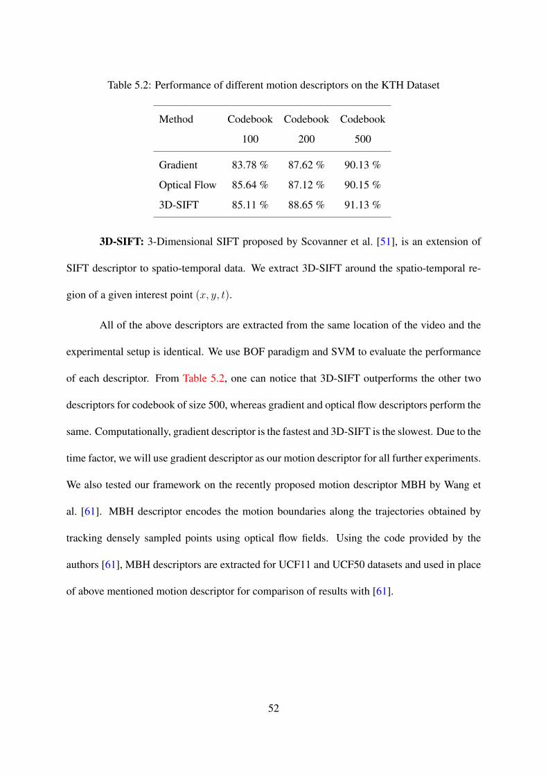
Table 5.2: Performance of different motion descriptors on the KTH Dataset
Method Codebook Codebook Codebook
100 200 500
Gradient 83.78 % 87.62 % 90.13 %
Optical Flow 85.64 % 87.12 % 90.15 %
3D-SIFT 85.11 % 88.65 % 91.13 %
3D-SIFT: 3-Dimensional SIFT proposed by Scovanner et al. [51], is an extension of
SIFT descriptor to spatio-temporal data. We extract 3D-SIFT around the spatio-temporal re-
gion of a given interest point (x, y, t).
All of the above descriptors are extracted from the same location of the video and the
experimental setup is identical. We use BOF paradigm and SVM to evaluate the performance
of each descriptor. From Table 5.2, one can notice that 3D-SIFT outperforms the other two
descriptors for codebook of size 500, whereas gradient and optical flow descriptors perform the
same. Computationally, gradient descriptor is the fastest and 3D-SIFT is the slowest. Due to the
time factor, we will use gradient descriptor as our motion descriptor for all further experiments.
We also tested our framework on the recently proposed motion descriptor MBH by Wang et
al. [61]. MBH descriptor encodes the motion boundaries along the trajectories obtained by
tracking densely sampled points using optical flow fields. Using the code provided by the
authors [61], MBH descriptors are extracted for UCF11 and UCF50 datasets and used in place
of above mentioned motion descriptor for comparison of results with [61].
52

5.2.1 Effect of increasing the action classes
In this experiment, we show that increasing the number of action classes affects the
recognition accuracy of a particular action class. Since the UCF11 dataset is a subset of UCF50,
we first start with the 11 actions from the UCF11 dataset and randomly add new actions from
the remaining 39 different actions from the UCF50 dataset. Each time a new action is added,
a complete leave-one-out cross validation is performed using bag of video words approach on
motion descriptor and SVM for classification on the incremented dataset using a 500 dimension
codebook. Performance using BoVW-SVM on the initial 11 actions is 55.46% and BoVW-NN
is 37.09%. Even with the increase in the number of actions in the dataset, SVM performs
significantly better than nearest neighbor approach.
Figure 5.1 shows the change in performance by using BoVW-SVM on the initial 11
actions as we add the 39 new actions, one at a time. Increasing the number of actions in the
dataset has affected some actions more than others. Actions like “soccer juggling” and “tram-
poline jumping” were most affected; they have a standard deviation of ∼7.08% and ∼5.84%,
respectively. Some actions like “golf swing” and “basketball” were least affected with a very
small standard deviation of ∼1.35% and ∼2.03%, respectively. Overall the performance on 11
actions from UCF11 dropped by ∼13.18%, i.e., from 55.45% to 42.27%, by adding 39 new
actions from UCF50. From Figure 5.1, one can also notice that 8 of 11 actions have standard
deviation of more than ∼4.10%. Analysis of the confusion table shows a huge confusion of
these initial 11 actions with newly added actions. This shows that the motion feature alone is
not discriminative enough to handle more action categories.
To address the above concerns, we propose a new scene context descriptor which is more dis-
53

Perfo
rman
ce (%
)
50
60
70
80 Basketball (mean:45.05%, SD: 2.03)Biking (mean:31.18%, SD: 4.41)Diving (mean:68.40%, SD: 2.30)GolfSwing (mean:72.75%, SD: 1.34)HorseRiding (mean:38.95%, SD: 1.34)SoccerJuggling (mean:34.15%, SD: 7.09)
Number of actions added
Perfo
rman
ce (%
)
20
30
40
1 5 9 13 17 21 25 29 33 37
Swing (mean:50.20%, SD: 4.50)TennisSwing (mean:46.00%, SD: 4.88)TrampolineJumping (mean:49.53%, SD: 5.84)VolleyballSpiking (mean:59.88%, SD: 4.88)WalkingWithDog (mean:28.03%, SD: 4.10)
Figure 5.1: The effect of increasing the number of actions on the UCF YouTube Action
dataset’s 11 actions by adding new actions from UCF50 using only the motion descriptor.
Standard Deviation (SD) and Mean are also shown next to the action name.
criminative and performs well in huge action datasets with a high number of action categories.
From the experiments on UCF50, we show that the confusion between actions is drastically re-
duced and the performance of the individual categories increased by fusing the proposed scene
context descriptor.
5.3 Scene Context descriptor
In order to overcome the challenges of unconstrained web videos, and handle a large
dataset with lots of confusing actions, we propose using the scene context information in which
the action is happening. For example, skiing and skate boarding, horse riding and biking, and
54

Playin
g Pian
oJum
p Rop
eFrame ‘n’ Frame ‘n+1’
Moving and Stationary Pixelsusing Optical Flow
Moving PixelsStationary Pixels
CSIFT on Moving Pixel
Jump R
ope
Ski je
t
CSIFT on Stationary Pixel
Figure 5.2: Moving and stationary pixels obtained using optical flow.
indoor rock climbing and rope climbing have similar motion patterns with high confusion, but
these actions take place in different scenes and contexts. Skiing happens on snow, which is very
different from where skate boarding is done. Similarly, horse riding and biking happen in very
different locations. Furthermore, scene context also plays an important role in increasing the
performance on individual actions. Actions are generally associated with places, e.g., diving
and breast stroke occur in water, and golf and javelin throw are outdoor sports. In order to
increase the classification rate of a single action, or to reduce the confusion between similar
actions, the scene information is crucial, along with the motion information. We refer to these
places or locations as scene context in our work.
As the number of categories increases, the scene context becomes important, as it helps
reduce the confusion with other actions having similar kinds of motion. In our work, we define
55

scene context as the place where a particular motion is happening (stationary pixels), and also
include the object that is creating this motion (moving pixels).
It has been shown that humans tend to focus on objects that are salient; This unique
capability helps improve object detection, tracking, and recognition. In general, humans tend
to focus on the things that are moving in their field of view. We try to mimic this by coming up
with groups of moving pixels which can be roughly assumed as salient regions and groups of
stationary pixels as an approximation of non-salient regions in a given video.
Moving and Stationary Pixels: Optical flow gives a rough estimate of velocity at each
pixel given two consecutive frames. We use optical flow (u, v) at each pixel obtained using
Lucas-Kanade method [40] and apply a threshold on the magnitude of the optical flow, to
decide if the pixel is moving or stationary. Figure 5.2 shows the moving and stationary pixels
in several sample key frames. We extract dense CSIFT [58] at pixels from both groups, and
use BOF paradigm to get a histogram descriptor for both groups separately. We performed
experiments using CSIFT descriptor, extracted on a dense sampling of moving pixels MPv
and stationary pixels SPv. For a 200 dimension codebook, the moving pixels CSIFT histogram
alone resulted in a 56.63% performance, while the stationary pixels CSIFT histogram achieved
56.47% performance on the UCF11. If we ignore the moving and stationary pixels and consider
the whole image as one, we obtain a performance of 55.06%. Our experiments show that
concatenation of histogram descriptors of moving and stationary pixels using CSIFT gives the
best performance of 60.06%. From our results, we conclude that concatenation of MPv and
SPv into one descriptor SCv is a very unique way to encode the scene context information.
For example, in a diving video, the moving pixels are mostly from the person diving, and the
56

stationary pixels are mostly from the water (pool), which implies that diving will occur only in
water and that this unique scene context will help detect the action diving.
Why CSIFT? : In [36], Liu et al. shows that using SIFT on the UCF11 dataset gave
them 58.1% performance. Our experiments on the same dataset using GIST gave us a very
low performance of 43.89%. Our approach of scene context descriptor using CSIFT gave us a
performance of 63.75%, ∼2.5% better than motion feature and ∼5.6% better than SIFT. It is
evident that color information is very important for capturing the scene context information.
Key frames: Instead of computing the moving and stationary pixels and their corre-
sponding descriptor on all the frames in the video, we perform a uniform sampling of k frames
from a given video, as shown in Figure 5.3. This reduces the time taken to compute the de-
scriptors, as the majority of the frames in the video are redundant. We did not implement any
kind of key frame detection, which can be done by computing the color histogram of frames
in the video and considering a certain level of change in color histogram as a key frame. We
tested on the UCF11 dataset by taking different numbers of key frames sampled evenly along
the video. Figure 5.4 shows that the performance on the dataset is almost stable after 3 key
frames. In our final experiments on the datasets, we consider 3 key frames equally sampled
along the video, to speed up the experiments. In this experiment, a codebook of dimension 500
is used.
5.3.1 How discriminative is the scene context descriptor?
In this experiment the proposed scene context descriptors are extracted, and a bag of
video word paradigm followed by SVM classification, is employed to study the proposed de-
57
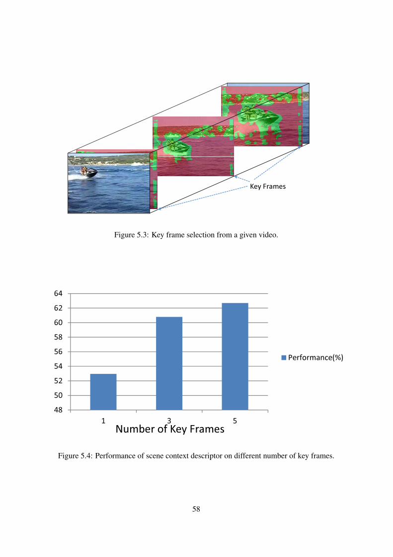
Key Frames
Figure 5.3: Key frame selection from a given video.
545658606264
Performance(%)
48505254
1 3 5Number of Key FramesFigure 5.4: Performance of scene context descriptor on different number of key frames.
58

30
40
50
60
70
80
90
100 Basketball (mean:45.0%, SD: 1.08)Biking (mean:59.08%, SD: 1.19)Diving (mean:91.13%, SD:2.50)GolfSwing (mean:62.78%, SD: 1.56)HorseRiding (mean:60.20%, SD: 2.73)SoccerJuggling (mean:8.13%, SD: 0.34)Swing (mean:46.05%, SD: 3.22)
Perfo
rman
ce (%
)
0
10
20
30
1 4 7 10 13 16 19 22 25 28 31 34 37 40
Swing (mean:46.05%, SD: 3.22)TennisSwing (mean:44.9%, SD: 3.02)TrampolineJumping (mean:67.78%, SD: 2.70)VolleyballSpiking (mean:78.93%, SD: 2.36)WalkingWithDog (mean:44.60%, SD: 4.10)
Number of actions added
Perfo
rman
ce (%
)
Figure 5.5: Effect of increasing the number of actions on the UCF YouTube Action dataset’s 11
actions by adding new actions from UCF50, using only the scene context descriptor. Standard
Deviation (SD) and Mean are shown next to the action name.
scriptor. Similar to the experiment in section 5.2.1, one new action is added to UCF11 in-
crementally from UCF50, at each increment leave-one-out cross-validation is performed. The
average performance on the initial 11 actions of UCF11, is 60.09%, after adding 39 new ac-
tions from UCF50 the performance on the 11 actions dropped to 52.36%. That is a ∼7.72%
decrease in performance, compared to ∼13.18% decrease for motion descriptor. The average
standard deviation of the performance of the initial 11 actions over the entire experimental
setup is ∼2.25% compared to ∼4.18% for motion descriptor. Figure 5.5 clearly shows that the
scene context descriptor is more stable and discriminative than the motion descriptor with the
increase in the number of action categories.
59

5.4 Fusion of descriptors
A wide variety of visual features can be extracted from a single video, such as motion
features (e.g., 3DSIFT, spatio-temporal features), scene features (e.g., GIST), or color features
(e.g., color histogram). In order to do the classification using all these different features, the
information has to be fused eventually. According to Snoek et al., [54] fusion schemes can be
classified into early fusion and late fusion based on when the information is combined.
Early Fusion: In this scheme, the information is combined before training a classi-
fier. This can be done by concatenating the different types of descriptors and then training a
classifier.
Late Fusion: In this scheme, classifiers are trained for each type of descriptor, then
the classification results are fused. Classifiers, such as support vector machines (SVM), can
provide a probability estimate for all the classes rather than a hard classification decision. The
concept of fusing this probability estimate is called Probabilistic Fusion [74]. For probabilis-
tic fusion, the different descriptors are considered to be conditionally independent. This is a
fair assumption for the visual features that we use in this work, i.e., motion descriptor using
gradients and Color SIFT. In probabilistic fusion the individual probabilities are multiplied and
normalized. For d sets of descriptors Xjd1 extracted from a video, the probability of the video
being classified as action a, i.e., p(a |Xjd1
), using probabilistic fusion is:
p(a |Xjd1
)=
1
N
d∏j=1
p (a |Xj) , (5.1)
where N is a normalizing factor which we consider to be 1. In late fusion, the individual
strengths of the descriptors are retained.
60

30
40
50
60
70
80
Code Book 200
Code Book 500
Perfo
rman
ce (%
)
0
10
20
30Code Book 1000
Code Book 1500
Perfo
rman
ce (%
)
Figure 5.6: Performance of different methods to fuse scene context and motion descriptors on
UCF50 dataset.
5.4.1 Probabilistic Fusion of Motion and Scene Context descriptor
Probabilistic Fusion: Late fusion using probabilistic fusion requires combining the
probability estimates of both the descriptors from their separately trained SVM’s, i.e.,
max (PSC(i) PM(i)) , where i = 1 to a,
where a is the number of actions to classify, and PSC(i) and PM(i) are the probability es-
timates of action i, using SVMs trained on scene context descriptors and motion descrip-
tors separately. We also tested early fusion of both motion and scene context features, i.e.,
[Mv SCv], and then trained an SVM, which gave ∼5% performance better than individual de-
scriptors on UCF50, which was expected. But, doing a early fusion after normalization, i.e.,
61

[Mv/max (Mv) , SCv/max (SCv)], gave a huge increase in the performance, about ∼14%. It
is evident from Figure 5.6, that on average across all the codebooks, late fusion (probabilistic
fusion) is the best. Therefore, in all of our experiments on the KTH, HMDB51, UCF YouTube
(UCF11), and UCF50 datasets, we do probabilistic fusion of both scene context and motion
descriptors.
5.5 System Overview
To perform action recognition, we extract the following information from the video: 1)
Scene context information in key frames and 2) motion features in the entire video, as shown
in Figure 5.7. The individual SVMs probability estimates are fused to get the final classifica-
tion. In the training phase we extract spatio-temporal features m1,m2, ..,mx, from x interest
points detected using the interest point detector proposed by Dollar et al. [12], from each of
the training videos. We also extract CSIFT features on moving pixels mp1,mp2, ..,mpy and
stationary pixels sp1, sp2, .., spz from k key frames in the video, where y and z are the num-
ber of CSIFT features extracted from moving and stationary regions, respectively. A codebook
of size p is generated of the spatio-temporal features from all the training videos. Similarly,
a codebook of size q is generated of CSIFT features from moving pixels and stationary pixels
combined. For a given video v, we compute the histogram descriptors Mv, MPv, and SPv
using their respective codebooks for the x spatio-temporal features from the entire video, y
CSIFT features from the moving pixels, and z CSIFT features from the stationary pixels from
key frames. We do an early fusion of MPv and SPv before training a classifier using support
vector machine (SVM), i.e., SCv = [MPv SPv], which we call the scene context descriptor.
62

Training Videos
Interest point
detector in the
entire video
Scene Context Descriptor
Selection of Key
frames (typically 3)
Optical Flow (u,v) on
Key frames
tvu ³+2 22
if
Moving Pixel Stationary Pixel
yes no
Extract CSIFT
descriptors on
Moving Pixels
Extract CSIFT
descriptors on
Stationary Pixels
Vocabulary learning
Histogram based
representation of
CSIFT descriptors
vMP
Histogram based
representation of
CSIFT descriptors
vSP
Concatenation of descriptors
from moving and stationary pixels][vv
SPMP
Motion Descriptor
Motion Feature
Extraction
Vocabulary
Learning
Histogram based
representation of
Motion features
vM
Train SVM Classifier (histogram
intersection kernel)
Train SVM
Classifier
(histogram
intersection
kernel)
Figure 5.7: Proposed approach.
63

We train SVM classifier SVMM for all the motion descriptors Mv, and separate SVM clas-
sifier SVMC for all scene context descriptors SCv, where v = [1, 2, , tr]; tr is the number
of training videos. Given a query video q, we extract the motion descriptor Mq and the scene
context descriptor SCq, as described in the training phase. We perform a probabilistic fusion of
the probability estimates of the motion descriptor [PM(1), PM(2), ., PM(a)], and scene context
descriptor [PSC(1), PSC(2), ., PSC(a)] obtained from SVMM and SVMC trained on motion
and scene context descriptors, respectively, for a action classes, i.e.,
[P (1), P (2), ., P (a)] =
[PM(1)PC(1), PM(2)PC(2), ., PC(a)PM(a)]
We use the fused probabilities as confidence to do the action classification.
5.6 Experiments and Results
Experiments have been performed on the following datasets: KTH, HMDB51, UCF11,
and UCF50. The KTH dataset consists of 6 actions performed by 25 actors in a constrained
environment, with a total of 598 videos. The HMDB51 dataset has 51 action categories, with a
total of 6849 clips. This dataset is further grouped into five types. In this dataset, general facial
action type is not considered as articulated motion, which leaves the dataset with 47 action
categories. UCF11 dataset includes 1100 videos and has 11 actions collected from YouTube
with challenging conditions, such as low quality, poor illumination conditions, camera motions,
etc. The UCF50 dataset has 50 actions with a minimum of 100 videos for each category,
also collected from YouTube. This dataset has a wide variety of actions taken from different
contexts and includes the same challenges as the UCF YouTube Action dataset.
64

In all of our experiments we used 3 key frames from a single video to extract scene
context features as explained before; however, we use all the frames in the video to get motion
features without any pruning. We don’t consider the audio, text, etc. contained in the video file
to compute any of our features. Our method uses only the visual features. All the experiments
have been performed under leave-one-out cross-validation unless specified.
5.6.1 UCF11 Dataset
This is a very challenging dataset. We extract 400 cuboids of size 11x11x17 for the
motion descriptor and a scene context descriptor from 3 key frames. We evaluate using leave-
one-out cross validation. Our approach gives a performance of 73.20%, with a codebook of size
1000. Motion descriptor alone gives a performance of 59.89%, and the scene context descriptor
alone gives a performance of 60.06%. The idea of scene context plays a very important role
in the performance of our approach. For example, the performance of motion descriptor for
biking action is 49%, and it has 21% confusion with horse riding. After fusion with scene
context descriptor, which has 12% confusion with horse riding, the performance increased to
67% and the confusion with horse riding reduced to 10%. The confusion decreased by 11%
and the performance increased by 18%. This happens due to the complementary nature of
probabilistic fusion where the individual strengths of the descriptors is preserved. This is also
observed in “basketball” and “tennis swing” as shown in Figure 5.8.
The performance reported by Liu et al [37] using hybrid features obtained by pruning
the motion and static features is 71.2%. We perform ∼2% better than Liu et al [37]. Recently,
Ikizler-Cinbis et al. [21] showed that their approach has 75.21% performance, which is∼2.1%
65

55 5 1 1 6 3 1 11 14 2
67 10 1 4 1 1 1 16
1 98 1 1
1 89 1 6 3 1
1 7 1 83 2 1 1 6
12 6 6 6 49 3 1 1 3 12
11 1 1 2 3 67 9 1 4
16 1 3 1 1 1 68 2 7
4 2 8 76 6 5
2 3 1 2 92 1
3 20 2 10 2 1 1 2 59
Basketball
Biking
Diving
GolfSwing
HorseRiding
SoccerJuggling
Swing
TennisSwing
TrampolineJumping
VolleyballSpiking
WalkingB
as
Bik
Div
Gol
Hor
Soc
Swi
Ten
Tra
Vol
Wal
Figure 5.8: Confusion table for UCF11 dataset using our approach.
better than our approach. However, they perform computationally intense steps like video
stabilization, person detector, and tracking, which are not done in our approach. By replacing
the motion feature with MBH [61] and following the exact same experimental setup [61],
the motion(MBH) and scene context descriptors gave us 83.13% and 46.57%, respectively.
The proposed probabilistic fusion gives 87.19%, which is ∼2.99% better than the best known
results on UCF11 as reported by Wang et al. [61].
66

5 10 15 20 25 30 35 40 45 50
5
10
15
20
25
30
35
40
45
50 0
10
20
30
40
50
60
70
80
90
Figure 5.9: Confusion table for UCF50 using our approach.
5.6.2 UCF50 Dataset
This is a huge and challenging dataset with 50 action categories. In this experiment,
1000 dimension codebooks are used for both the motion and scene context descriptor. The
individual performance of motion descriptor is 53.06%; using our new scene context descriptor
the performance is 47.56%. After the fusion of both the descriptors we have a performance of
68.20%, which is a ∼15% increase.
67

The performance on rock climbing indoor using motion descriptors is 28%, 11% of the
time it gets confused with rope climbing, and 10% of the time rope climbing gets confused
with rock climbing indoor. This is understandable because of the similar motion pattern in
these actions. The performance of scene context descriptor for indoor rock climbing is 71%
with a confusion of 1% with rope climbing, and the performance of rope climbing is 10% with
a confusion of 4% with indoor rock climbing. Low confusion occured because both the actions
happened in two very different locations. Using our approach we get 80% performance on
indoor rock climbing and 42% performance on rope climbing. The complete confusion table
is shown in Figure 5.9. In some cases, the scene context descriptor performs badly compared
to motion descriptor; for example, in bench press the performance using scene context is 54%
with 15% confusion with pizza tossing. The reason for this is that both the actions are per-
formed indoor in most cases. However, they have no confusion in motion descriptor. This
increases the final performance of bench press to 71%.
Figure 5.10 shows the performance by incrementally adding one action at a time from
UCF50 to UCF11. The overall performance for the initial 11 actions using our approach is
70.56%, and on all the 50 actions it is 66.74%, a drop of 3.8% in the overall performance in
spite of adding 39 new actions. The fusion of both the descriptors consistently added 15.5% to
the motion descriptor with a variance of 1%, and 17.3% to the scene context descriptor with a
variance of 9.3%.
It is interesting to note that substituting MBH as the motion descriptor in the above
experimental setup gave us the best performance of 76.90%, where MBH and scene context
descriptors gave 71.86% and 47.28%, respectively.
68

5.6.3 HMDB51 Dataset
The proposed approach has been tested on all the 51 categories in HMDB51 dataset on
original videos, and the experimental setup was kept similar to [28] for comparison. We used
the HOG/HOF features provided by the authors [28], which gave us 19.96% for a codebook
of size 2000. The scene context descriptor is computed by extracting dense CSIFT on 3 key
frames and quantizing using a codebook of size 2000, which gave us 17.91%. The proposed
fusion has 27.02%, which is∼3.84% higher than the best results reported by Kuehne et al. [28].
5.6.4 KTH Dataset
We applied our proposed method on the KTH dataset. Although the idea of scene
context is not useful in this dataset, experiments have been conducted simply to compare the
performance of our method with other state-of-the-art results on the KTH dataset. The experi-
mental setup is leave-one-out cross validation and a 1000 dimension codebook is used. We got
a performance of 89.79% using our approach, whereas scene context feature alone performed
64.20% and motion feature alone performed 91.30%. We had a 1.51% drop in the performance
due to the scene context features, in spite of the 25.95% difference between scene context and
motion features. This shows the robustness in doing the probabilistic fusion of both scene
context and motion descriptors.
69

Table 5.3: Performance comparison on KTH dataset
Method Acc(%) Method Acc(%)
Our method 89.79 % Liu, et al. [37] 91.3 %
Dollar, et al. [12] 80.6 % Wong, et al. [68] 83.9 %
5.7 Summary
In this chapter we proposed an approach to do action recognition in huge datasets like
UCF50 and HMDB51. The proposed approach has the best performance on datasets like
UCF11 (87.19%), UCF50 (76.90%) and HMDB51 (27.02%). We showed that, as the num-
ber of categories increase, the motion descriptors become less discriminative. We also showed
that the proposed scene context descriptor is more discriminative, and when properly fused
with motion descriptors gives∼15% and∼4% improvement on UCF50. Our approach doesn’t
require pruning of motion or static features, stabilization of videos, or detection and tracking of
persons. The proposed method has the ability to do action recognition on highly unconstrained
videos and also on large datasets.
Particle Flow Field is slow and has not been tested here due to the large volume of the
datasets. But when tested on the smaller dataset UCF11 it gives ∼ 2% better performance
compared to using 3D-Gradients to generate motion descriptor with a codebook of size 1000.
Bag of Video Words framework has some inherent disadvantages and are addressed in
the next chapter.
70

01020304050607080 Performance (%) 0
Scen
e Con
text F
eatu
reM
otion
Featu
rePr
opos
edM
ethod
New
actio
ns ra
ndom
ly ad
ded t
o UCF
YouT
ube D
atase
t
Figure 5.10: Performance as new actions are added to UCF YouTube (UCF11) Dataset from
the UCF50 dataset.
71

CHAPTER 6: INCREMENTAL ACTION RECOGNITION
6.1 Introduction
In the field of computer vision, bag of features (BOF) is receiving increasing attention
due to its simplicity and surprisingly good performance on object, scene and action recognition
problems [13] [15] [38] [30] [69] [53]. Inspired by the success of the bag of words approach
in text categorization [4] [19], computer vision researchers have widely and successfully ap-
plied the bag of visual words model beyond BOF for visual recognition. It is generally a
two-stage procedure, consisting of vocabulary construction and category model learning (e.g.
with SVM). Since visual words are not intrinsic entities, it suffers from effective vocabulary
construction problems. Different vocabulary construction methods may lead to very different
performance. In general, there are two types of visual vocabularies. The most common one is
the flat vocabulary, which is normally created by applying k-means on the subsamples of the
training data [13] [30] [69] [15]. Although approaches employing such vocabularies have, in
general, obtained good performance, this method for generating vocabularies is computation-
ally expensive, mainly due to the cost of clustering of training visual features and assigning
the visual descriptors to visual words (especially for generating very large vocabularies). Hi-
erarchical vocabularies constructed using hierarchical clustering techniques [45] [42] or an
72

ensemble of randomized trees [43] [71] have been explored recently, and have been proven to
be very efficient and effective in visual recognition.
However, we argue that most current bag of visual words approaches may not be very
useful for solving realistic problems in practice. One problem is that these approaches are not
easily scalable. This is due to the fact that most current visual vocabularies are constructed
using a predefined training dataset, which is static in nature. However, this may not be the case
in most real world problems, since the datasets are dynamically changing. For instance, if we
want to extend the bag of visual words method which obtains good results on KTH dataset [29]
to solve a bit more difficult problem, we have to face two cases: one is that we want to add
more training examples of the “waving” action into the dataset since we have to slightly change
the definition of “waving” so that the system can recognize more types of “waving”; another
case is that we need to train the system to recognize a new action category. For both cases,
the existing vocabulary is not suitable for handling the new situation. Hence, both the visual
vocabulary and computed histograms (bag of visual words) have to be updated.
Besides, as we know, given a patch from an image, we can sometimes correctly guess
the content of the image. Yet bag of visual words approaches are not able to predict given
only a few features. Therefore, these approaches are not robust to large occlusion. For action
recognition, they do not have the capability to perform recognition on a frame by frame basis.
Furthermore, bag of visual words methods cannot deal with videos containing multiple actions
happening simultaneously. they can only classify videos with a single action.
In this chapter, we propose an indexing based approach “Feature-Tree”. We first use
SR-tree (Sphere/ Rectangle) [24] to generate our feature-tree using the features of the labeled
73

training examples. SR-tree is a variant of R-tree [18], which has been accepted as a standard
by the industry. Instead of splitting the high-dimensional feature space by hyper-plane as in
earlier tree techniques, the feature points are organized into regions in the feature space, which
are specified by the intersection of a bounding sphere and bounding rectangle. Hence, SR-tree
can maintain smaller region volume to provide disjoint regions and larger diameter to support
fast range and NN search in high-dimensional space. During the recognition phase, we extract
features from an unknown action video and classify each feature into an action category using
SR-tree. To recognize the action, we adopt a simple voting method by counting the labels of
the features.
The rest of the chapter is organized as follows. Section 6.2 presents our proposed
method. The experiments are discussed in section 6.3. Finally, we conclude this chapter in
section 6.4.
6.2 Proposed method
In this section, we describe our proposed method in detail. Figure 6.1 shows the pro-
cedure of action recognition using our feature-tree. There are two phases: Figure 6.1 top row
depicts the procedure of growing the feature-tree and Figure 6.1 bottom row describes the
recognition steps. In the feature-tree growing stage, local spatiotemporal features are detected
and extracted from each labeled video, and then each feature is represented by a pair [d, l]
where d is the feature descriptor and l is the class label of the feature. Finally, we index all
the labeled features using SR-tree. In the recognition stage, given an unknown action video,
we first detect and extract local spatiotemporal features, and then for each feature we launch
74

a query into the feature-tree. A set of nearest neighbor features is returned. An action is rec-
ognized by simple weighted voting from all the neighbor features. The entire procedure does
not require intensive training. Therefore, we can easily apply incremental action recognition
with the feature-tree. Besides, we also can easily localize the actions in the video, and detect
multiple actions occurring simultaneously in the same video.
6.2.1 Feature Extraction
In order to detect the action in a given video, we use the spatiotemporal interest point
detector proposed by Dollar et al. [13]. Compared to the 3D Harris-Corner detector [29], it
produces dense features that can significantly improve the recognition performance in most
cases. It utilizes 2-D Gaussian filter and 1-D Gabor filters separately in spatial and temporal
directions respectively. A response value is given by the following function at every position
(x, y, t):
R = I ∗ gσ(x, y) ∗ hev(t)2 + I ∗ gσ(x, y) ∗ hod(t)2, (6.1)
where gσ(x, y) is the spatial Gaussian filter, hev and hod are a quadrature pair of the 1-D Gabor
filter in time. It produces high responses to the temporal intensity change points. The interest
points N are selected at the locations of local maximal responses, and 3D cuboids are extracted
around them. For simplicity, we use the flat gradient vectors di ∈ RN to describe the cuboids
with PCA being utilized to reduce the descriptor dimension, so a video is represented by a set
of cuboids D = di.
75

Figure 6.1: The framework of action recognition using feature-tree.
76

Figure 6.2: Tree structure defined by the intersection of bounding spheres and bounding rect-
angles.
6.2.2 Feature-tree Growing
Given a set of action videos V = v1, v2, . . . , vM and its corresponding class label
li ∈ 1, 2, . . . , C, we extracted n spatiotemporal features dji (1 ≤ j ≤ n) from video vi. We
associated each feature with its class label and get a two-elements feature tuple xji = [dji lc].
Then we obtained a collection of labeled features T = xji to construct our feature-tree.
SR-tree is chosen to index the labeled feature collection T . It is a disk-based data struc-
ture having successfully integrated the advantages of the R-tree and SS-tree data structures, so
it is fast for large scale datasets which cannot be fit into the main memory. We briefly review
77

its data structure as follows. Figure 6.2 shows the nested hierarchy structure with a root node,
nodes, and leaves. Instead of splitting the feature space by a hyper plane, SR-tree organizes
the data by hierarchical regions. The region is defined by the intersection of a bounding sphere
(the smallest sphere covering a set of points) and a bounding rectangle. This design creates a
balance between having larger region diameter and smaller region volume to improve the per-
formance of nearest neighbors search. Each leaf of an SR-tree has a minimum and maximum
limit on the number of entries it can take. Entries in the leaf store the points with their labels.
A leaf is split and converted into a node if it reaches the maximum number of allowed entries.
Nodes do have a limit on the number of children they can hold. Each entry in a node has
four components: bounding sphere, bounding rectangle, number of points in the sub-tree, and
pointers to all its children. We can consider the regions in our feature-tree as a cluster of feature
points which are spatially close to each other. We can imagine the same type of actions share
lots of feature patterns, so each leaf node might have dominated class labels. The feature-tree
can grow in three steps:
1. Inserting a new feature point into the tree.
2. Splitting a leaf when it is overcrowded.
3. Reinserting the feature points from the step 2.
Insertion: A centroid-based algorithm is applied in the insertion algorithm due to its
effectiveness for nearest neighbor queries. The insertion algorithm is supposed to find the best
sub-tree that can accommodate the new spatiotemporal feature point xji from T . The sub-tree,
whose centroid (i.e. the center of the feature points covered by it) is nearest to xji , is selected.
78

After insertion, the regions (the bounding sphere and the bounding rectangle of the parents) are
updated. In fact, it propagates the region updates upwards till it reaches the root. The bounding
rectangle is updated the same way as it is done in R-tree. The bounding sphere, however, is
updated using both the bounding sphere and bounding rectangle of its children. Using both
the bounding sphere and bounding rectangle of the children helps the radius of the parent’s
bounding sphere to be smaller compared to the SS-tree, which in turn reduces the overlap of
the bounding spheres.
Splitting: If a leaf is overcrowded, a portion of its entries are reinserted. If the reinser-
tion fails, it is split and converted into a node and the entries are reinserted.
Deletion: An entry is simply removed if the deletion of the entry causes no under-
utilization of any leaf or node. If the deletion does cause under-utilization of a leaf or node, the
leaf or node is removed from the tree and the orphaned entries are reinserted into the tree.
6.2.3 Action Recognition
Given the feature-tree, the action recognition starts by extracting spatiotemporal fea-
tures from an unknown action video. Suppose the query action video is represented by a bag
of spatiotemporal features, say Q = dq(1 ≤ q ≤ M), our recognition task is to find its
class label. Instead of using complicated training or inference method, we adopt simple voting
schema.
For each query feature dq, we retrieve the K nearest neighbors from the feature-tree,
and we assign a class label to it based on the label voting of the K returned features. Then,
the label of Q is decided by the final voting of the class labels of the query features in Q. As
79

we know, generally the query features of Q may contain good and bad features (good feature
meaning discriminative features). In order to distinguish the voting from them, we can assign
a class label to Q using the following equation:
C = arg maxC
M∑q=1
K∑r=1
τ ∗ Irq‖dq − dqr‖+ε
(6.2)
where dqr ∈ NN(dq), Irq is a indicator which is equal to 1 if the label of dr is C, is otherwise
zero, and ε, τ are constant number (NN - Nearest Neighbor). Therefore, the contribution
of each feature also depends on how well it matches the query feature. Noisy features (bad
features) usually do not have good matches.
The nearest neighbor search algorithm implements an ordered depth first traversal.
First, it collects the candidate set, and secondly it revises the candidate set by visiting each
leaf having its region intersected with the candidate set. The search is terminated if there are
no more leaves to visit and the final candidate set is the search result. The search is performed
by computing the distance of the search point xji to the region of the child and visiting the child
which is closer. Since the region for an SR-tree is the intersection of a bounding sphere and
a bounding rectangle, the minimum distance from a search point to a region is defined as the
maximum between the minimum distance to the bounding sphere and the minimum distance to
the bounding rectangle. We summarize the nearest search procedure and the action recognition
steps in Table 6.1 and Table 6.2.
6.3 Experiments and results
We tested our approach on two publicly available dataset: the KTH dataset [69] and
the IXMAS multi-view dataset [63]. The default experiment settings are as follows, unless
80

Table 6.1: Nearest Neighbor Search.
Objective: Given a query point, find the nearest neighbors
1. Start with the candidate set nearest to the query point dq.
2. Search each leaf having its region intersecting the candidate set.
3. Start with the leaf closest to the query point dq.
4. If K nearest neighbors dr are found terminate.
5. If not, go to the next closest leaf having its region intersecting
the candidate set and do this till all the K nearest
neighbors are found.
Table 6.2: Main steps of Action recognition using feature-tree.
Objective: Given a query video Q, assign a class label to it.
Feature Extraction:
1. For a given video Q, detect the spatiotemporal interest points using
the Dollar detector and extract the cuboids around them.
2. Compute gradient for each cuboid q, and use PCA to reduce the dimension,
then it is represent by a descriptor dq.
3. Representing Q as a bag of features dq
Action Recognition:
Given the query features of Q : dq
1. For each query feature dq in Q retrieve the nearest neighbor dqr
2. The class label of Q is decided by equation 6.2:
C = arg maxC∑M
q=1
∑Kr=1
τ∗Irq‖dq−dqr‖+ε
81

Figure 6.3: Some examples of KTH dataset actions.
and until otherwise specified. For each video we extract 200 cuboids. Gradient based feature
descriptor is used in all the experiments.
6.3.1 Experiments on the KTH Dataset
We applied our approach to the KTH dataset, which contains six actions: boxing, clap-
ping, waving, jogging, walking, and running. They are performed by 25 actors under four
different scenarios of illumination, appearance, and scale changes. In total it contains 598
video sequences. Figure 6.3 shows some examples from the dataset.
In our experiment we constructed the feature-tree using 5 persons and using the remain-
ing 20 persons for testing. This procedure was repeated five times by switching the persons
for feature-tree growing and experimental testing. The average accuracy was 87.8%. Instead
of using SR-tree data structure to grow our feature-tree as we describe in section 6.2, we use
Random Forest [7] to create the feature-trees using 5 persons, and test it on the rest 20 per-
sons. As before, we repeated five times. Each time, there are 50 random feature-trees, and the
final classification was made by voting from all the feature-trees. The average accuracy was
72.9%. As we know, Random Forest uses binary trees which separate the feature space by a
82

77.5 6.3 16.3 0.0 0.0 0.0
35.4 50.6 13.9 0.0 0.0 0.0
6.3 1.3 92.5 0.0 0.0 0.0
0.0 0.0 1.3 15.0 70.0 13.8
0.0 0.0 1.3 5.0 93.8 0.0
0.0 0.0 5.0 5.0 8.8 81.3
Boxing
Clapping
Waving
Jogging
Running
Walking
Boxing Clapping Waving Jogging Running Walking
Figure 6.4: Confusion table on KTH data set for 5 persons used in Random Forest.
plane when splitting the space at each node to construct the feature-trees. It might be weaker
than our proposed feature-tree constructor which separates the feature space by regions. We
also did similar experiments using vocabulary-based approach which use k-means to gener-
ate the flat vocabulary, and use SVM to train the category model. The average accuracy was
about 84.4%. We also observed that the increase in training examples had little effect on the
performance. When we increase the training set to 10 persons the performance using SR-tree
structure increases to 90.3%.
83

91.3 6.3 1.3 0.0 0.0 1.3
8.9 84.8 6.3 0.0 0.0 0.0
7.5 0.0 92.5 0.0 0.0 0.0
0.0 0.0 0.0 83.8 6.3 10.0
0.0 0.0 0.0 13.8 85.0 1.3
0.0 0.0 0.0 1.3 0.0 98.8
Boxing
Clapping
Waving
Jogging
Running
Walking
WalkingRunningJoggingWavingClappingBoxing
Figure 6.5: Confusion table on KTH data set for 5 persons used to grow feature-tree.
Figure 6.4 and Figure 6.5 show the confusion table on KTH dataset using our feature-
tree and Random Forest. From the confusion tables provided in Figure 6.5, one can observe
that the actions clapping and waving are confused with boxing, and there is a lot of confusion
between jogging and running. It’s observed that the hand movement actions get confused
between one another. This is also the case with leg movement actions; this is due to the
similarity between the actions. This has also been observed in approaches like bag of video
84

Table 6.3: The performance of the different bag of visual words approaches.
Method Acc(%) Method Acc (%)
Our method 90.3 Neibles, et al. [44] 81.5
Liu, et al. [38] 91.3 Dollar, et al. [13] 80.6
Wong, et al. [69] 83.9 Schuldt, et al. [50] 71.7
words. The Random Forest approach has a high rate of confusion with actions like jogging
with running.
We list the state-of-the-art results on the KTH dataset using bag of visual words related
approaches in Table 6.3. We cannot directly compare them due to different experiment settings.
For example, [38] and [63] used 24 persons for training. We do not list some results which are
reported by using spatiotemporal information.
Particle Flow Field: Using particle flow field (PFF) instead of 3D-Gradients inside the
extracted 3D-Cuboids as mentioned in section 6.2.1, the performance on KTH dataset increases
by ∼ 4%, ie., 93.98% compared to 90.3% using 3D-Gradients.
6.3.2 Effect of number of Features, feature dimensions and Nearest Neighbors
Without exception, in all our experiments, we extracted 200 spatiotemporal features
from each video, and used 1 nearest neighbor for voting in the feature query phase. In these
experiments, we tried to verify how the performance is affected by the number of extracted
features and the K value in K nearest neighbors. Figure 6.6 shows the results of using different
number of features and different K value. It is very impressive that using 10 features we can
85

75
80
85
90
95
10 Features
20 Features
50 Features
Acc
ura
cy (
%)
55
60
65
70
1 NN 10 NN 20 NN 30 NN 40 NN 50 NN
50 Features
100 Features
200 Features
Acc
ura
cy (
%)
Number of nearest neighbors (NN)
Figure 6.6: Performance comparison of using feature-tree on spatiotemporal features. The
number of features is increased from 10 to 200 and the nearest neighbor search is increased
from 1 to 50.
still get about 75% average accuracy. It does not make too much difference when the number
of extracted feature is larger than 100.
It implies that feature-tree performs well even if only very few features points are avail-
able from each video. As the number of feature point’s increase to 200, the performance
increases to about 89%.
Effect of feature dimension: For feature dimension of 100 we have a performance
of 87.8% and we achieve almost the same with dimension of 50 i.e., 87.7%. Reduction in
dimension of the feature vector has very less impact on the performance, which can be helpful
to decrease the computations needed.
86

6.3.3 Incremental action recognition
In the real world we need systems which can adapt to or learn from the dynamic envi-
ronment. Most vocabulary-based bag of feature methods cannot cope with this situation, since
they normally need intensive training for vocabulary model or category model. However, our
feature-tree method can make it. In our approach the feature-tree can be update with new train-
ing examples or new categories without reconstructing the entire tree. In this experiment we
again use the KTH data set to show the advantages of having an incremental feature-tree. We
train our tree with the first 5 people on 4 actions (boxing, clapping, waving, walking). We add
one person at a time from action 5 to the feature-tree, and check the effect of incrementing.
The test data set in this experiment is from 5 actions and the remaining 20 people not included
in the training set. The results are shown in Figure 6.7. Incrementing tree is done by inserting
the new feature points into the fully grown tree. We increment the tree with features from 5
more persons for action 5 (Jogging), which is previously not included in the training set. From
our experiment we observe that the performance increases as the tree is incremented with new
training data.
6.3.4 Recognizing multiple actions in a video
As the aforementioned, the basic bag of visual words approaches are unable to detect
and localize the actions when multiple instances happen in the same video. However, our
feature-tree can be used to easily handle this case. Given a video with multiple actions, we ex-
tracted m spatiotemporal features from it. We conducted feature queries and assigned a class
label to each of them. We ranked then by the class frequency fc. If fc > Ω (a predefined thresh-
87

84
86
88
90
Performance (%)
78
80
82
1st Person 2nd Person 3rd Person 4th Person 5th Person
Performance (%)
Figure 6.7: Plot shows the effect on recognition performance with incremental examples from
the new category added into the feature-tree.
old) then we can recognize the action and localize it by the locations of the voting features. To
simulate this scenario and demonstrate this straightforward method, we created a video with
two instances: boxing and walking from the KTH dataset by simply concatenate them by the
height edge. Figure 6.8 shows the localization and recognition. All red features are assigned
with boxing, while the blue ones are running. We extract the feature points from each video
and merge then in to a single query file. We query the tree constructed using 5 persons and
6 actions training dataset. The above two videos for query are not in the training. Figure 6.8
shows the results.
6.3.5 Action Recognition in frame by frame mode
In this experiment, we proved that action recognition can be done in a frame-by-frame
mode. It means for an online system, the recognition does not need to wait for the last minutes
88

Side View Front View
Boxing
Walking
Misclassification
Boxing
Walking
Misclassification
ClassificationGround TruthClassificationGround Truth
Figure 6.8: Classification and localization of two actions happen in the same video. The red
features are classified into boxing, and blue is walking.
of the video. We can make the decision and update it with more frames coming. Obviously,
vocabulary-based approaches cannot be conducted in a frame-by-frame mode, since the his-
togram will be meaningful when enough observations have been made on a number of frames.
In order to verify this function, we created a feature-tree with five persons. And then we test
on the rest of videos in frame-by-frame mode. Figure 6.9 shows the results for all the actions.
It clearly shows the system can achieve good performance with very few frames like 3 frames.
The recognition performance will be stable after frame 11. After this, more coming frames
cannot help improve the performance. The recognition is even faster than real-time. In our
system, each feature query takes about 0.02s and each frame has about at most 10 features, and
totally less than 0.2s/frame.
89

Acc
ura
cy
Number of Frames
Acc
ura
cy
Figure 6.9: Performance by increasing the number of frames considered in voting.
6.3.6 Experiments on IXMAS Multi-view dataset
We also applied our method on the IXMAS multi-view dataset. The dataset contains
13 daily life actions, performed three times by 12 actors under four different views. In total
it contains 1848 video sequences. This data is challenging due to the variations in the camera
view, and it also has very similar actions like checking watch, scratching head, and pointing.
Here we conduct two different sets of experiments:
Learning from four views: In the first experiment, learning is done from four views.
We take the videos from 5 actors to construct the feature-tree and the rest 7 actors for testing.
The experiments were repeated four times with videos from different actors to grow the feature-
tree. First, we recognized the action using single view, and average accuracies for each camera
1-4 are 69.6%, 69.2%, 62.0%, 65.1%. This is a little better than that in paper [63], but it is
worse than results reported in [38]. However, both of them using videos from ten actors for
90

training, but we only used 5 actors. Besides, both of them need intensive training process.
Next, we tried to recognize actions using simple voting on four views, and we can improve the
total average accuracy to about 72.6%. Figure 6.10 shows the confusion table for it. Actions
like sit-down, get up, turn around, kicking and pickup has an average performance of 89%, but
the performance is bad on the other actions.
Learning from three views: In the second experiment, we consider to use videos from
three camera views to construct the feature-tree, and the fourth camera view to test the system.
This is repeated four times by changing the camera-views in the training and testing set. In
this experiment with a camera view missing, we achieved an accuracy of 81.0% 70.9% 79.2%
64.9% for camera 1 2 3 4 respectively. The performance is better than that results reported
in [63] and [38].
6.4 Summary
In this chapter, we proposed a framework for incremental action recognition using
feature-tree. Our system does not require detection and tracking of humans and does not need
intensive training (vocabulary training and category model training), but we still can get com-
petitive performance and fast recognition. The system is very practical since we can handle
incremental action recognition and index the feature-tree with disk-based SR-tree data struc-
ture. Our system has very good scalability. Most importantly, our system can recognize mul-
tiple actions happening in a video simultaneously. Using particle flow fields gives the best
performance on KTH dataset.
91

85.7 0.0 0.0 0.0 0.0 4.8 0.0 0.0 0.0 0.0 9.5 0.0 0.0
47.6 42.9 0.0 0.0 0.0 4.8 0.0 0.0 0.0 0.0 4.8 0.0 0.0
14.3 9.5 66.7 0.0 0.0 4.8 0.0 0.0 0.0 0.0 4.8 0.0 0.0
0.0 0.0 0.0 100 0.0 0.0 0.0 0.0 0.0 0.0 0.0 0.0 0.0
0.0 0.0 0.0 0.0 100 0.0 0.0 0.0 0.0 0.0 0.0 0.0 0.0
0.0 0.0 0.0 0.0 0.0 95.2 4.8 0.0 0.0 0.0 0.0 0.0 0.0
0.0 0.0 0.0 0.0 0.0 0.0 100 0.0 0.0 0.0 0.0 0.0 0.0
14.3 19.0 4.8 0.0 0.0 9.5 4.8 33.3 0.0 0.0 9.5 0.0 4.8
9.5 0.0 0.0 0.0 0.0 9.5 23.8 0.0 38.1 4.8 14.3 0.0 0.0
0.0 0.0 0.0 0.0 0.0 4.8 4.8 0.0 0.0 90.5 0.0 0.0 0.0
14.3 4.8 4.8 4.8 4.8 33.3 0.0 0.0 0.0 0.0 33.3 0.0 0.0
0.0 0.0 0.0 4.8 0.0 0.0 0.0 0.0 0.0 0.0 0.0 95.2 0.0
0.0 0.0 0.0 0.0 0.0 0.0 0.0 0.0 0.0 9.1 27.3 9.1 54.5
cw ca sh sd gu ta wa hw pu ki po pu th
get up
sit down
scratch head
cross arms
check watch
trun around
walk
hand wave
punch
kick
pick up
throw (head)
point
Figure 6.10: Performance by increasing the number of frames considered in voting.
92

CHAPTER 7: CONCLUSION AND FUTURE WORK
The main theme of this dissertation has been low-level video representation that is
robust and can perform reasonably well in different action recognition scenarios. The scenarios
that typically arise in action recognition datasets are: 1) Scenario where the human detection
and tracking can be performed on the given video, 2) Scenario where the human can be detected
but is difficult to track, 3) Videos where foreground and background separation is easier than
detecting and tracking objects of interest and 4) Finally, videos where any pre-processing is
challenging.
We propose a new low-level video representation “Particle Flow Field” obtained using
optical flow and particle advection. In order to handle different action recognition scenarios:
first, we propose 3D-spatio temporal volumes where the object of interest can be detected and
tracked, second, a scene context descriptor is introduced where the foreground and background
can be separated, and finally, a feature-tree is proposed to do real-time incremental action
recognition where none of the pre-processing is done.
7.1 Summary of Contributions
The primary contributions of this thesis are outlined below:
1. Low-level video representation
93

(a) Introduction of “Particle Flow Field” as a robust low-level video representation.
(b) Representation of video in terms of particle flow fields.
(c) Application of particle flow field for action recognition in a bag of video words
framework.
(d) Best performance using particle flow field compared to 2D-Gradients, 3D-Gradients,
and Optical Flow.
2. Action recognition using 3D-spatio temporal volumes
(a) Introduction of the histogram of oriented 3D-Gradients (3D-STHOG) for action
recognition in 3D-spatio temporal volumes.
(b) Investigation of the sensitivity of 3D-STHOG to change in scale, frame rate, and
translation.
(c) The proposed 3D-STHOG has been tested on videos taken from aerial, rooftop, and
ground cameras.
(d) Introduction of the histogram of oriented particle flow (3D-STHOPFF) fields for
action recognition in 3D-spatio temporal volumes.
(e) The proposed 3D-STHOPFF is suitable for human action recognition without track-
ing humans.
(f) Demonstrated best performance using 3D-STHOPFF.
3. Action recognition using scene context in web videos
(a) Provided insight into the challenges of large scale action recognition datasets.
94

(b) Proposed the use of moving and stationary pixel information to obtain a scene con-
text descriptor.
(c) Introduced a scene context descriptor that helps improve performance in large scale
datasets.
(d) Proposed the idea of early fusion schema for descriptors obtained from moving and
stationary pixels to understand the scene context, and finally perform a probabilistic
fusion of the scene context descriptor and motion descriptor.
4. Incremental action recognition using feature-tree
(a) Introduced a framework that does not require re-training with the addition of new
action categories or videos.
(b) Proposed the use of the SR-Tree in action recognition frame work to perform in-
cremental action recognition.
(c) Feature-tree framework has the ability to perform multiple action recognition, frame-
by-frame action recognition, and can localize actions.
(d) Algorithm to perform real-time action recognition using feature-tree.
7.2 Future Directions
In this section, we present some possibilities for future directions to further the research
carried out in this dissertation.
In chapter 3, particle flow field was proposed, which is computationally expensive com-
pared to other video representations. Instead of interpolating the optical flow, median filter can
95

be used to improve the accuracy and speed. Significant camera motion can hurt the perfor-
mance of particle flow field. In videos with significant camera motion, the motion of the
particle will have the camera motion embedded in it, which is irrelevant for action recognition.
Low rank optimization can be used to remove the camera motion from the particle motion.
The same approach can be used to accurately separate moving and stationary pixels, in order
to generate scene context descriptors proposed in chapter 5.
Future efforts can focus on human detection and detecting human body parts in a video
using particle flow fields. The use of particle flow fields in crowd behavior analysis can also be
explored.
96

LIST OF REFERENCES
[1] S. Ali and M. Shah. A lagrangian particle dynamics approach for crowd flow segmen-tation and stability analysis. In Computer Vision and Pattern Recognition, 2007. CVPR’07. IEEE Conference on, pages 1 –6, june 2007.
[2] J.S. Beis and D.G. Lowe. Indexing without invariants in 3d object recognition. PatternAnalysis and Machine Intelligence, IEEE Transactions on, 21(10):1000 –1015, oct 1999.
[3] J.L. Bentley. Multidimensional binary search trees in database applications. SoftwareEngineering, IEEE Transactions on, SE-5(4):333 – 340, july 1979.
[4] David M. Blei, Andrew Y. Ng, and Michael I. Jordan. Latent dirichlet allocation. J.Mach. Learn. Res., 3:993–1022, March 2003.
[5] Aaron F. Bobick and James W. Davis. The recognition of human movement using tem-poral templates. IEEE Trans. Pattern Anal. Mach. Intell., 23:257–267, March 2001.
[6] O. Boiman, E. Shechtman, and M. Irani. In defense of nearest-neighbor based imageclassification. In Computer Vision and Pattern Recognition, 2008. CVPR 2008. IEEEConference on, pages 1 –8, june 2008.
[7] Leo Breiman. Bagging predictors. Machine Learning, 24:123–140, 1996.10.1023/A:1018054314350.
[8] Claudette Cedras and Mubarak Shah. Motion-based recognition: A survey. Image andVision Computing, 13:129–155, 1995.
[9] C.C. Chen and J.K. Aggarwal. Recognizing human action from a far field of view. InIEEE Workshop on Motion and Video Computing, 2009.
[10] N. Dalal and B. Triggs. Histograms of oriented gradients for human detection. In CVPR,2005.
[11] Jia Deng, Alexander C. Berg, Kai Li, and Li Fei-Fei. What does classifying more than10,000 image categories tell us? In Proceedings of the 11th European conference onComputer vision: Part V, ECCV’10, pages 71–84, 2010.
[12] P. Dollar, V. Rabaud, G. Cottrell, and S. Belongie. Behavior recognition via sparse spatio-temporal features. In Visual Surveillance and Performance Evaluation of Tracking andSurveillance, 2005. 2nd Joint IEEE International Workshop on, pages 65 – 72, oct. 2005.
[13] P. Dollar, V. Rabaud, G. Cottrell, and S. Belongie. Behavior recognition via sparse spatio-temporal features. In IEEE PETS, 2005.
97

[14] L. Fei-Fei and P. Perona. A bayesian hierarchical model for learning natural scene cate-gories. In Computer Vision and Pattern Recognition, 2005. CVPR 2005. IEEE ComputerSociety Conference on, volume 2, pages 524 – 531 vol. 2, june 2005.
[15] L. Fei-Fei and P. Perona. A bayesian hierarchical model for learning natural scene cate-gories. In Computer Vision and Pattern Recognition, 2005. CVPR 2005. IEEE ComputerSociety Conference on, volume 2, pages 524 – 531 vol. 2, june 2005.
[16] Lena Gorelick, Moshe Blank, Eli Shechtman, Michal Irani, and Ronen Basri. Actions asspace-time shapes. IEEE Trans. PAMI, 2007.
[17] A. Gupta, A. Kembhavi, and L.S. Davis. Observing human-object interactions: Usingspatial and functional compatibility for recognition. IEEE Trans. PAMI, 2009.
[18] Antonin Guttman. R-trees: a dynamic index structure for spatial searching. SIGMODRec., 14(2):47–57, June 1984.
[19] Thomas Hofmann. Unsupervised learning by probabilistic latent semantic analysis. InMachine Learning, page 2001, 2001.
[20] Pengyu Hong, Thomas S. Huang, and Matthew Turk. Gesture modeling and recognitionusing finite state machines. In Proceedings of the Fourth IEEE International Conferenceon Automatic Face and Gesture Recognition 2000, FG ’00, pages 410–, 2000.
[21] Nazli Ikizler-Cinbis and Stan Sclaroff. Object, scene and actions: combining multiplefeatures for human action recognition. In Proceedings of the 11th European conferenceon Computer vision: Part I, ECCV’10, 2010.
[22] G Johansson. Visual perception of biological motion and a model for its analysis. Atten-tion Perception Psychophysics, 14(2):201–211, 1973.
[23] Imran N. Junejo, Emilie Dexter, Ivan Laptev, and Patrick Perez. Cross-view action recog-nition from temporal self-similarities. In ECCV, ECCV ’08, Berlin, Heidelberg, 2008.Springer-Verlag.
[24] Norio Katayama and Shin’ichi Satoh. The sr-tree: an index structure for high-dimensional nearest neighbor queries. In Proceedings of the 1997 ACM SIGMOD inter-national conference on Management of data, SIGMOD ’97, pages 369–380, New York,NY, USA, 1997. ACM.
[25] Norio Katayama and Shin’ichi Satoh. Experimental Evaluation of Disk-Based DataStructures for Nearest Neighbor Searching. In Data Structures, Near Neighbor Searches,and Methodology: Fifth and Sixth DIMACS Implementation Challenges, volume 59 ofAMS DIMACS Series, pages 87–104. AMS, 2002.
[26] Yan Ke, R. Sukthankar, and M. Hebert. Spatiotemporal shape and flow correlation foraction recognition. In CVPR, 2007.
98

[27] Alexander Klser, Marcin Marszalek, and Cordelia Schmid. A spatio-temporal descriptorbased on 3d-gradients. In BMVC, 2008.
[28] H. Kuehne, H. Jhuang, E. Garrote, T. Poggio, and T. Serre. Hmdb: a large video databasefor human motion recognition. In Proceedings of the International Conference on Com-puter Vision (ICCV), 2011.
[29] I. Laptev and T. Lindeberg. Space-time interest points. In ICCV, 2003.
[30] I. Laptev, M. Marszalek, C. Schmid, and B. Rozenfeld. Learning realistic human actionsfrom movies. In CVPR, 2008.
[31] I. Laptev, M. Marszalek, C. Schmid, and B. Rozenfeld. Learning realistic human actionsfrom movies. In Computer Vision and Pattern Recognition, 2008. CVPR 2008. IEEEConference on, pages 1 –8, june 2008.
[32] I. Laptev, M. Marszalek, C. Schmid, and B. Rozenfeld. Learning realistic human actionsfrom movies. In Computer Vision and Pattern Recognition, 2008. CVPR 2008. IEEEConference on, pages 1 –8, june 2008.
[33] Ivan Laptev. On space-time interest points. Int. J. Comput. Vision, 64(2-3):107–123,September 2005.
[34] V. Lepetit, P. Lagger, and P. Fua. Randomized trees for real-time keypoint recognition.In Computer Vision and Pattern Recognition, 2005. CVPR 2005. IEEE Computer SocietyConference on, volume 2, pages 775 – 781 vol. 2, june 2005.
[35] Ce Liu, W.T. Freeman, E.H. Adelson, and Y. Weiss. Human-assisted motion annotation.In Computer Vision and Pattern Recognition, 2008. CVPR 2008. IEEE Conference on,pages 1 –8, june 2008.
[36] Jingen Liu, Jiebo Luo, and M. Shah. Recognizing realistic actions from videos ”in thewild”. In Computer Vision and Pattern Recognition, 2009. CVPR 2009. IEEE Conferenceon, pages 1996 –2003, june 2009.
[37] Jingen Liu and Mubarak Shah. Learning human actions via information maximization.In Computer Vision and Pattern Recognition, 2008. CVPR 2008. IEEE Conference on,pages 1 –8, june 2008.
[38] Jingen Liu and Mubarak Shah. Learning human actions via information maximization.In Computer Vision and Pattern Recognition, 2008. CVPR 2008. IEEE Conference on,pages 1 –8, june 2008.
[39] David G. Lowe. Distinctive image features from scale-invariant keypoints. Int. J. Com-put. Vision, 60(2):91–110, November 2004.
[40] Bruce D. Lucas and Takeo Kanade. An iterative image registration technique with anapplication to stereo vision. In Proceedings of the 7th international joint conference onArtificial intelligence - Volume 2, pages 674–679, 1981.
99

[41] Ramin Mehran, Brian E. Moore, and Mubarak Shah. A streakline representation of flowin crowded scenes. In European Conference on Computer Vision(ECCV), 2010.
[42] K. Mikolajczyk and H. Uemura. Action recognition with motion-appearance vocabularyforest. In Computer Vision and Pattern Recognition, 2008. CVPR 2008. IEEE Conferenceon, pages 1 –8, june 2008.
[43] F. Moosmann, Bill Triggs, and Frederic Jurie. Fast Discriminative Visual Codebooksusing Randomized Clustering Forests. In J. Platt B. Scholkopf and T. Hoffman, edi-tors, Advances in Neural Information Processing Systems 19, pages 985–992, Vancouver,Canada, 2007. MIT Press.
[44] J.C. Niebles and Li Fei-Fei. A hierarchical model of shape and appearance for humanaction classification. In Computer Vision and Pattern Recognition, 2007. CVPR ’07.IEEE Conference on, pages 1 –8, june 2007.
[45] D. Nister and H. Stewenius. Scalable recognition with a vocabulary tree. In ComputerVision and Pattern Recognition, 2006 IEEE Computer Society Conference on, volume 2,pages 2161 – 2168, 2006.
[46] S. Oh and et al. A large-scale benchmark dataset for event recognition in surveillancevideo. In CVPR, 2011.
[47] R. Poppe. A survey on vision-based human action recognition. Image and Vision Com-puting, 2010.
[48] K.K. Reddy, J. Liu, and M. Shah. Incremental action recognition using feature-tree. InICCV, 2009.
[49] M.D. Rodriguez, J. Ahmed, and M. Shah. Action mach a spatio-temporal maximumaverage correlation height filter for action recognition. In CVPR, 2008.
[50] Christian Schldt, Ivan Laptev, and Barbara Caputo. Recognizing human actions: A localsvm approach. In In Proc. ICPR, pages 32–36, 2004.
[51] Paul Scovanner, Saad Ali, and Mubarak Shah. A 3-dimensional sift descriptor and itsapplication to action recognition. In Proceedings of the 15th international conference onMultimedia, MULTIMEDIA ’07, pages 357–360, 2007.
[52] Paul Scovanner, Saad Ali, and Mubarak Shah. A 3-dimensional sift descriptor and itsapplication to action recognition. In Multimedia, MULTIMEDIA ’07, 2007.
[53] J. Sivic, B.C. Russell, A.A. Efros, A. Zisserman, and W.T. Freeman. Discovering ob-jects and their location in images. In Computer Vision, 2005. ICCV 2005. Tenth IEEEInternational Conference on, volume 1, pages 370 – 377 Vol. 1, oct. 2005.
[54] Cees G. M. Snoek, Marcel Worring, and Arnold W. M. Smeulders. Early versus latefusion in semantic video analysis. In Proceedings of the 13th annual ACM internationalconference on Multimedia, MULTIMEDIA ’05, pages 399–402, 2005.
100

[55] Yang Song, Ming Zhao, J. Yagnik, and Xiaoyun Wu. Taxonomic classification for web-based videos. In Computer Vision and Pattern Recognition (CVPR), 2010 IEEE Confer-ence on, pages 871 –878, june 2010.
[56] A. Torralba and A. Efros. Unbiased look at dataset bias. In CVPR, 2011.
[57] P. Turaga, R. Chellappa, V.S. Subrahmanian, and O. Udrea. Machine recognition ofhuman activities: A survey. IEEE Trans. Circuits and Systems for Video, 2008.
[58] K.E.A. van de Sande, T. Gevers, and C.G.M. Snoek. Evaluating color descriptors forobject and scene recognition. Pattern Analysis and Machine Intelligence, IEEE Transac-tions on, 32(9):1582 –1596, sept. 2010.
[59] Ashok Veeraraghavan, Amit K. Roy-Chowdhury, and Rama Chellappa. Matching shapesequences in video with applications in human movement analysis. IEEE Trans. PatternAnal. Mach. Intell., 27(12):1896–1909, December 2005.
[60] H. Wang, M.M. Ullah, A. Klaser, I. Laptev, and C. Schmid. Evaluation of local spatio-temporal features for action recognition. In BMVC, 2009.
[61] Heng Wang., Alexander Klaser., and Cheng-Lin Liu. Action recognition by dense trajec-tories. In Computer Vision and Pattern Recognition, 2011. CVPR 2011. IEEE Conferenceon, 2011.
[62] Zheshen Wang, Ming Zhao, Yang Song, S. Kumar, and Baoxin Li. Youtubecat: Learningto categorize wild web videos. In Computer Vision and Pattern Recognition (CVPR),2010 IEEE Conference on, pages 879 –886, june 2010.
[63] D. Weinland, E. Boyer, and R. Ronfard. Action recognition from arbitrary views using 3dexemplars. In Computer Vision, 2007. ICCV 2007. IEEE 11th International Conferenceon, pages 1 –7, oct. 2007.
[64] Daniel Weinland, Remi Ronfard, and Edmond Boyer. A survey of vision-based methodsfor action representation, segmentation and recognition. Comput. Vis. Image Underst.,115:224–241, February 2011.
[65] G. Willems, T. Tuytelaars, and L. Van Gool. An efficient dense and scale-invariant spatio-temporal interest point detector. In ECCV, Berlin, Heidelberg, 2008. Springer-Verlag.
[66] A.D. Wilson and A.F. Bobick. Parametric hidden markov models for gesture recognition.Pattern Analysis and Machine Intelligence, IEEE Transactions on, 21(9):884 –900, sep1999.
[67] J. Winn, A. Criminisi, and T. Minka. Object categorization by learned universal visualdictionary. In Computer Vision, 2005. ICCV 2005. Tenth IEEE International Conferenceon, volume 2, pages 1800 –1807 Vol. 2, oct. 2005.
101

[68] Shu-Fai Wong, Tae-Kyun Kim, and R. Cipolla. Learning motion categories using bothsemantic and structural information. In Computer Vision and Pattern Recognition, 2007.CVPR ’07. IEEE Conference on, pages 1 –6, june 2007.
[69] Shu-Fai Wong, Tae-Kyun Kim, and R. Cipolla. Learning motion categories using bothsemantic and structural information. In Computer Vision and Pattern Recognition, 2007.CVPR ’07. IEEE Conference on, pages 1 –6, june 2007.
[70] Shandong Wu, Omar Oreifej, and Mubarak Shah. Action recognition in videos ac-quired by a moving camera using motion decomposition of lagrangian particle trajec-tories. Computer Vision, IEEE International Conference on, 0:1419–1426, 2011.
[71] T. Yeh, J. Lee, and T. Darrell. Adaptive vocabulary forests for dynamic indexing andcategory learning. In Computer Vision, 2007. ICCV 2007. IEEE 11th International Con-ference on, pages 1 –8, oct. 2007.
[72] Alper Yilmaz and Mubarak Shah. Actions sketch: A novel action representation. Com-puter Vision and Pattern Recognition, IEEE Computer Society Conference on, 1:984–989,2005.
[73] Alper Yilmaz and Mubarak Shah. A differential geometric approach to representing thehuman actions. Comput. Vis. Image Underst., 2008.
[74] Yan-Tao Zheng, Shi-Yong Neo, Tat-Seng Chua, and Qi Tian. Probabilistic optimizedranking for multimedia semantic concept detection via rvm. In Proceedings of the 2008international conference on Content-based image and video retrieval, CIVR ’08, pages161–168, 2008.
102