acoustic emission simulation for online impact detection

Acoustic Emission Simulation for Online Impact Detection

C. Yang, M. A. Torres-Arredondo, Claus-Peter Fritzen

University of Siegen, Germany

October 26-28, 2011, Stuttgart

Institut für Mechanik und Regelungstechnik - Mechatronik Prof. Dr.-Ing. C.-P. Fritzen

UNIVERSITÄT SIEGEN

Outline

Introduction Feature extraction Gaussian Process (GP) Simulation Results

1/16

Introduction Feature extraction Gaussian Process Simulation Results

Impact Damage in Aeronautic and Aerospace Structures Courtesy of NASA

Impact in Metallic Structures Courtesy of SLODIVE

Impact is a common source of in-service damage that compromises the safety and

performance of engineering structures (civil engineering, automobile, aeronautics…) Online impact detection systems are essential and require automatic and intelligent

techniques providing a probabilistic interpretation of their diagnostics.

Machine learning algorithms generally require huge amount of data, in order to make the process cost-effective, simulation of impacts has been performed to get the training data set from modeling.

2/16

Movitation:


• Step1: Obtain the training data f(x,y)

• Step2: Signal processing and feature vectors construction

• Step3: Gaussian Models construction and Optimization

• Step4: Estimate f(x,y) for new inputs

Feature Extraction Model

Training Set Generation

Data Base Generation Feature Extraction

Dimension Reduction Features Vectors Generation

Model Generation Model Optimization

Unknown Impact Force

Predictions Fmax

Impact Location (x,y)

Predictions

Sensors

Random Impacts Feature Extraction

Sensor1 Sensor2 ... SensorJ

Sensor x Time

1 K 2K JK

Exp

erim

ents

3/16

General method:

Multiresolution Analysis (MRA)

Two Channel Subband Coder

Determine the entropy content of each level a with coefficients Wa=(wa,1, wa,2,…,wa,n)

Select the level with the minimum entropy value for optimal decomposition

, ,1

lnn

a a k a kk

E W W W

The purpose of using the DWT is to benefit from its localization property in the time and frequency domains (Mallat, 1989)

Relevant features can be extracted for improvement of future inferences

d3 (fmax/2,fmax)/4 an

(0,fmax)/2n

d2 (fmax/2,fmax)/2

a2 (0,fmax/2)/2

a1 (0,fmax/2)

x(t)

d1 (fmax/2,fmax)

...


4/16


Dimension Reduction: Nonlinear Principal Component Analysis

Multilayered perception architecture and auto-associative topology

Retain k principal components based on hierarchical error (Scholz et al., 2008)

Inputs are the approximation coefficients provided by MRA (dimension d)

NLPCA Architecture

Output forced to equal Input

1 1,2 1,2,...,...Total kE E E E

2

1

1ˆ ˆN

k k k kk

EdN

x x x x

Every space (k-1) is of minimal Error

Sensor1 Sensor2 ... SensorJ

Sensor x Coefficients

1 K 2K JK

Exp

erim

ents

Exp

erim

ents

Coefficients Sensors

5/16


Model Generation: Regression with Gaussian Processes (GP)

f (•) modelled by GP with zero mean and covariance matrix K

0,p f D K~ Ν

Data set D of D-dimensional training input vectors xi

Training vector t with noisy training targets ti = f (xi) + ε for i =1,...,N

New input vector xN+1

Predictions for noise-free output targets f (xN+1)

Steps

Optimize parameters Θ controlling K

Inverse

analysis method

Collect measured

responses of a body

Estimation from new responses

GP modelling allows to directly define the space of admissible functions relating inputs to outputs by simply specifying the mean and covariance functions of the process (Rasmussen&Williams,2006;Bishop,2007).

6/16

Covariance Function Selection The covariance in our case is squared exponential with automatic relevance

determination (ARD) distance measure defined by

T2 1( , ) exp

2ij i j i j i jk

K x x x x M x xM: diag (λ1,...λD)-2

λ: Input dimension length scale σ2: Signal Variance λ and σf are hyperparameters Θ

The learning task correspond to tuning the parameters of the covariance

function of the process The unknown parameters Θ in the covariance functions are calculated by

maximizing the negative logarithmic marginal likelihood A conjugate gradient optimization technique with line-search is used for this

purpose

T 1N 1 1log | log(2 ) log2 2 2

p t x K t K tL


7/16


T 11 N

2 T 11 N

N

N k

-

-

x k C t

x k C k

In the Gaussian Process framework, one can define a joint distribution over the observed training targets at the test location as

2N

1 T 20, 0,n

Nn

pck

T

C kK I kt

kkN N

tN+1: (t1,...,tN,tN+1)T σn

2: Noise Variance K: N×N matrix k: N×1 matrix btn. test and training targets k: Training target Variance I: Identity matrix

Predictions:

After optimization of the model:

Predictions for new values of x can be made

A predictive distribution over t is obtained The GP formulae for the mean and variance of the predictive distribution with the covariance function is given by

8/16


Experimental setup:

Plate specification: - Aluminum - 800mm*800mm - Thickness: 2mm

Sensor specification: - PIC255 from PI ceramic - Diameter: 10mm - Thickness: 0.2mm

Impact hammer specification: - Impact hammer type 8204 - Tip diameter: 2.5mm

9/16


Impact force description: The impact force is in fact a discontinue function, in time-dependent problems, it may

lead the time-stepping algorithm into problems when running .

To avoid the problems of discontinuity, smoothed step functions without overshoots are chosen to describe the impact force. Heaviside function flc2hs in Comsol is applied. It is a smoothed Heaviside function

with a continuous second derivative without overshoot.

)],(2),(2[max fallwidthrise tttflchttflchFf

)/()max( 2max mN

sFF

impact

F : maximum force (2-5N) : contacting area with the impact hammer impacts

2)2

35.2(

esimpact

10/16


Piezoelectric effect simulation (Piezo plane strain module)

The piezoelectric sensor function is the governing equation:

kSijklikli ESeD

3,2,1,,, lkji , ikle Sij

iD kE: piezoelectric constantv : dielectric constant

: electric displacement : electric field

Two dimensional model and boundary conditions:

The piezoelectric material constants are offered by PI Ceramic.

sensor1 sensor2 sensor3 sensor4

Mechanical boundary conditions: free Electrical boundary conditions: - Contacting layer of sensors with the plate: - Otherwise: zero charge

Impact Impact …… ……

ground

11/16


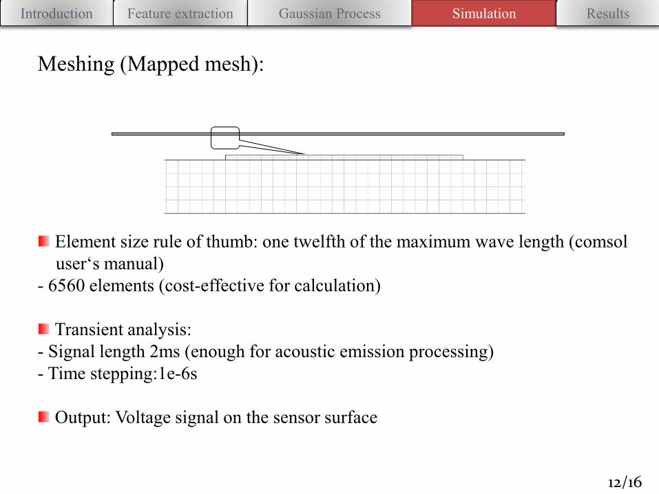
Meshing (Mapped mesh):

Element size rule of thumb: one twelfth of the maximum wave length (comsol user‘s manual) - 6560 elements (cost-effective for calculation) Transient analysis:

- Signal length 2ms (enough for acoustic emission processing) - Time stepping:1e-6s

Output: Voltage signal on the sensor surface

12/16


Results of an example (Impact applied in the middle of the plate)

sensor1 sensor2 sensor3 sensor4 Impact

The simulated sensor signals track well with the experimental signals The model is in 2D, in reality the wave will disperse. Compared with a 3D model, this 2D model is cost-effective, which saves calculation time

and memory consumption, and is enough for future impact magnitude estimation. 13/16

0 1 2 3 4 5 6 7

x 10-4

-5

-4

-3

-2

-1

0

1

2

3

4

5

Time (s)

Vo

lta

ge

(V

)

Sensor 1

Experimental Signal

Numerical Signal

0 0.5 1 1.5 2 2.5 3 3.5 4 4.5 5

x 10-4

-4

-2

0

2

4

6

8

10

12

Time (s)

Vo

lta

ge

(V

)

Sensor 2

Experimental Signal

Numerical Signal


Model trained with impacts between 2-5N at random locations

Training impacts with a grid density of 50mm. A single output Gaussian Process is proposed for impact magnitude

estimation. The feature vectors which are the GP inputs comprise:

- The difference in time of arrivals between the sensors

- The non-linear principal components extracted from the DWT

- The area under the curve of the power spectral density

14/16


Grey bars show the mean of the Gaussian process predictive distribution

Error bars correspond to plus and minus 2 standard deviations (95%)

The GP was able to estimate the impact magnitude force with an average percentage error of 8%

15/16

Results:

0 5 10 15 20 25 300

0.5

1

1.5

2

2.5

3

3.5

4

4.5

5

Test Number

Impa

ct F

orce

[N]

ExperimentEstimated


Conclusion: The proposed methodology has allowed to accurately estimate the magnitude of impact events in a simple structure.

The finite element simulation is very cost-effective to get the training set. The sensor signals from the model track well with the experimental data.

Pending:

Investigate the method applicability in more realistic and complex structures and materials Investigate the effect of different type of impacts in the prediction capabilities

16/16

Thank you for your attention! Question?

The authors are grateful to the IPP and MOSES programs of the center of sensor systems in University of Siegen for the financial support of this research work.

acoustic emission simulation for online impact detection

Documents