ACKNOWLEDGEMENTS

It is a pleasure to acknowledge the advice, guidance and continuous encouragement given by my supervisor, Prof H. Kleinpoppen, throughout the course of my research and during the preparation of this thesis, who has at all times an interest in my work.

I would like particularly to thank Prof P. G. Burke, who by permitting me to work with his group and his help and encouragement, during my stay in the Department of Applied Mathematics and Theoretical Physics at the Queen's University of Belfast, has rendered possible to successful completion of this thesis.

I wish to record my indebtedness for the help received from other members of staff and research students in the Department of Applied Mathematics and Theoretical Physics at the Queen's University of Belfast and in the Department of Physics at Stirling University. Thanks also due to Dr's K. Blum and C. Noble for their useful discussion.

I must also offer my heart-felt thanks to my wife and all the members of my family in Egypt for their unfailing support and sincere love.

Last, but no means least, financial support by the Egyptian Government is gratefully acknowledged.

CONTENTS

Page

ABSTRACT

INTRODUCTION

CHAPTER I BASIC CONCEPTS

1.1 Matrix Representation of the DensityOperator

1.2 Stokes' Parameters1.3 Irreducible Spherical TensorsI.if State and Integrated State Multipoles1.5 Orientation Vector and Alignment Tensor1.6 Spin Eigenvectors and Spin Tensors1.7 Vector Model and Symmetry Properties of

Diatonic Molecules

CHAPTER II RELATIVISTIC EFFECTS IN LOW ENERGY ELECTRON- ATOM SCATTERING AND SPIN POLARIZATION

II. 1 Dirac Wave Equation and the Breit Interaction11.2 Choice of the Atomic Target States11.3 Calculation of R-Matrix and K-Matrix II.^ Description of Electron Spin Polarization,

Cross sections and Scattering Asymmetry by Density Matrices

CHAPTER III POLARIZATION PHENOMENAL OF RADIATION

13

33

111.1111.2

111.3

lllAIII.5

Description of the Collision Expansion of the Integrated State Multipoles

in Terms of the Reduced Density Matrix Effect of Perturbation on the Decaying

ProcessRadiactive Decay of an Excited Atom Stokes' Parameters Description of the Emitted

Radiation

CHAPTER IV ELECTRON SCATTERING BY DIATOMIC MOLECULES 55

IV.1 Born-Oppenheimer and Fixed-Nuclei Approximations IV.2 Representation of the Nuclear Motion (Rotation

and Vibration)IV. 3 Exchange and Polarization PotentialsI V M e t h o d s of solution of The Scattering Process

CHAPTER V DISCUSSION AND NUMERICAL RESULTS 66

V. l Low-Energy Scattering of Electrons by CaesiumAtoms^^»^^

V.2 Stokes' Parameter for Inelastic Electron-Caesium Scattering^^ 65

V.3 Vibrational Inelastic Scattering of Electron by N2

r e fe r e n c e s 81

ABSTRACT

The relativistic R-matrix rnethod is used to calculate elastic and

inelestic cross sections for electrons incident on caesium atoms with

energies frcxn 0 to 3 eV, In addition to the total cross sections,

results are presented on the differential cross section, o r , and the

spin polarization, P^, of the scattered electrons as a function of

energy at eight scattering angles (10°, 30°, 50°, 70°, 90°,

110°, 130°, 150°). Also the differential cross section, spin

polarization and the left-right asyiimetry function, A , ares

calculated as a function of the scattering angles at a number of

chosen values of energies. The calculation reveals a wealth of2 2resonances around p; and P 3 thresholds. The resonances are

I . . . 2analysed in detail and their role in the scattering process is

discussed.

The density matrix formalism is used to derive expressions for

the Stokes' Parameters to describe the state of the photons emitted in

electron-atom collision experiment. Numerical results for the Stokes

Parameters of the light emitted in the decay 6p ^p 3 -> 6s ^S,2 ^

in atomic caesium after electron impact excitation are presented and

compared with the available measurements. These results show what

effects can be expected and may be useful for the planning of future

experiments.

The angular distribution and the integrated cross sections have

been calculated at incident electron energies 20, 25 and 30 eV, in

e-N^ scattering. The calculations are based on the use of numerical

basis functions in the R-f1atrix method, and exchange and polarization

effects are included. Also variation of the mixing parameter, between

p- and f- partial waves and the individual eigenphases with the

internuclear distance are presented. The mixing parameter has shown

to be a rapidly varying function of the internuclear distance

contradicting the assumption made by Chang (1977).

INTRODUCTION

Electrons play a central part in atomic and molecular physics.

Because of their small mass, electrons are much more active than the

nuclei in this microscopic world. Knowledge of the behaviour of

electrons is essential in understanding a large variety of problems such

as gaseous electronics, fusion plasmas, ionospheres, auroras, stellar

atmospheres and interstellar gases.

The outcome of electron-atom or electron-molecule collision

processes is studied through scattering experiments under some suitable

arrangements and physical conditions. Those physical conditions which

determine what approximation scheme should be applied incorporating

with the quantum theory of scattering. However, the theoretical

treatment of electron-molecule collision has features as distinct from

those of the electron-atom collision. This makes the solution of the

electron-molecule system more complicated than the electron-atom one.

These complications arise because the molecules have rotational and

vibrational degrees of freedom, the electron-molecule interactions is

essentially multicentered and nonspherical and lastly molecular targets

can dissociate in collision with an electron.

In recent years there has been an increasing interest, both

experimental and theoretical in the low energy scattering of electrons

by heavy atoms and by molecules. In this contribution we present some

recent theoretical results on the scattering of low energy electrons

from heavy atomic targets, caesium, and on the scattering of electrons

by N2- molecule at intermediate energies.

Following some important concepts which form the basis of the

theory in chapter I, chapter II contains a fuller discussion on the

relativistic R-matrix theory and expressions for the total and

differential cross sections. Spin polarization and scattering asymmetry

are also given. In chapter III the density matrix formalism is applied

to describe the polarization state of the photons emitted from a heavy

atom excited by electron impact. Methods of solution of the electron-

molecule collision problem and the approximations used are briefly

presented in chapter IV. In chapter V we discuss some implications of

our work and illustrate their usefulness through numerical calculations.

CHAPTER I

BASIC CONCEPTS

Throughout this chapter we present some important concepts

which form the basis of the theory.

>•1 Matrix Representation of The Density Operator

The dynamical state of a system must no longer be represented

by a unique vector, but by a statistical mixture of vectors. If the

dynamical state of a quantum system is completely known (one has

succeeded in determining precisely the variables of one of the complete

sets of compatible variable associated with the system) it is said to be

in a pure state. States which are not pure are called mixed states or

mixtures. Mixtures are states identified by less than maximum

information, ie are not described by a single wavefunction. Therefore

in order to describe mixed states the density operator is introduced

12 3 by the expression

P = S I i = 1, 2,1 J- 1 1

(U -1 )where Wj are the probabilities for the system being in a set of pure

states . In particular for a pure state |'F> the density operator

turns out to be

4'x'l'(1.1-2)

In general the density matrix element can be deduced from equation

(I»l-1), by sandwiching it between the two states of interest, as follows:

P fj =

= T. a ., W, a .,i k k j k(U -3 )

where can be expanded in terms of a set of orthogonal basis

I v * I " ik I Va .i-* )

For our purpose we lay down some properties^ of the density operator

(i) the density operator is a positive definite, hermitian operator of

trace euqal to unity.

(ii) For a mixed state, the following relation holds

2 2 tr p < (t r p) ,

whereas only for a pure state, we have

2 2 tr p = ( t r p)

(iii) For any observable quantity A the expectation value <A> is related

to p through the equation

<A> = 1^- Pàtr p

(iv) In the representation p is given by

(U -5 )

P = i1 + P P - iP \

z X y )P +iP 1-P /

X V z /

(U -4 )

where Pj , Py, P , are the cartesian components of the polarization

vector and where the two-by-two unit matrix and the Pauli spin

matrix are defined as

■ - i ; i l • , - C i j - i i s LThe main virtue of the density matrix is its analytical power in the

construciton of general formulae and in proving general theorems. In

fact, the specification of this operator is sufficient to determine all

physically measureable quantities. This procedure has the advantage of

providing uniform treatment for the pure states and the mixtures.

1 -2 Stokes Parameters

In the decay of an excited atomic state the emitted photons

may be observed in the direction of the unit vector with polar

angles 0^, <|) with respect to the collision system x, y, z, figure (1).

Due to the transverse nature of the electromagnetic waves the

polarization vector of photons is characterised by two linearlyA

independent basis vectors e t, and C2 in a plane perpendicular to n , as follows; ^

^2 ^where Cj , and ¿2 pointing in the direction of increasing 9 and

respectively.

The three basis vectors n^, e j, and &2 define a coordinate system

called the detector frame with as a quantization axis. The Stokes'

parameters are defined with respect to this detector frame in the

following:

(i) The total intensity I of the emitted photons

I = 1(0°) + 1(90°) = + 1(135°) = I(RHS) + I(LHS)(1 -2)

(ii) The degree of linear polarization with respect to x- and y- axes

^ 1(0°) - 1(90°)1 (0°) + 1(90°)

(U -3 )

(iii) The degree of linear polarization with respect to two orthogonal

axes oriented at degrees to the x- axis

n = 1(45°) - 1(135°) 1(45°) + 1(135°)

(1^-4)

where I( a°) is the fraction of intensity of a given beam which has

passed a linear polarizer with transmisión axis at angle a ° to the axis

° 1*

(iv) The degree of circular polarization n 2

„ _ I(RHS) - KLHS)'2 ■ -----------------

I(RHS) + I(LHS)(1^-5)

where I(RHS) (I(LHS)) is the intensity of right (le ft) handed circularly

polarized light.

In matrix notation the Stokes' parameters are grouped in the

matrix form

i f l * '’2^X'X 2 I

\-n .-in

-n.

3 '1(1.2-^)

where is the matrix element of the density operator P, X' (X) is the

halicity, taking values ^ 1. The normalization to the relevant intensity

is chosen by the relation

t rPx ' X=I (1.2-7)

Using the normalization condition (1.2-7) and the fact that the matrix

(1.2-6) is hermitian, we find only three parameters nj, n 2» ^3

linearly independent.

*•3 Irreducible Spherical Tensors

The subject of irreducible tensor operators occupies a central

position in the modern theory of angular momentum. When the angular

symmetries of the ensemble of interest are important it is convenient

to expand the density matrix operator p in terms of a basis set of

operators defined by its transformation properties under changes of the

coordinate system, these changes are rotations and inversions. Such a

set of operators are the irreducible tensor operators. This method

provides a well developed and efficient way of using the inherent

symmetry of the system. It also enables the consequences of angular

momentum conservation to be simply allowed for. Furthermore, one

can separate the dynamical and geometrical factors in the equations of

interest, without much effort, by using the "Wigner-Eckart Theorem".

A general tensor operator T| of rank K is defined as a quantity

represented by (2K + 1)- components, T| q , which transform according

to the irreducible representation of a rotation group by the

transformation equation ^

q (1.3-1)

where (a3y) are the Euler angles, the rotation operator R takes the old

system, unprimed, to the new system, primed, and D(a6y are the

matrix elements of R in the KQ- representation. Therefore, the tensor

Tj transforms like a spherical harmonic of order K.

Consider now a degenerate energy level of the physical system

which may include states with different angular momentum quantum

numbers j, j', ... . It is convenient to construct the set of tensor

operators T(j'pKQ angular momentum states by applying the

usual angular momentum coupling roles, in the form:

T(j'j)^„ - EZ (j’MlJ-M |KQ)|j’M:><jMjM.M! J J J JJ Jwhere,

| j- j ’ + j '

(IJ-2)

-K<Q$K

and |KQ) is the well-known Clebsch-Gordan coefficient.

Beside the transformation property under rotation, equation (1.3-

l)f the irreducible tensor operators have the following important

properties:

(i) the orthogonality property is defined as

5_ 6. . ,Kk Qq jj'

- (-1 ) ' T( j ' j ) ^_ . q

(1.3-3)

where is the hermitian adjoint of T(j'j)j^Q.

(ii) Matrix elements of the irreducible tensor operators between any pair

of desired states have a property known as the "Wigner-Eckart

Theorem". Namely, that the matrix elements with equal values of j, j'

and K, but with different Mj and Mj' and Q bear fbced ratios to one

another. These ratios depend on j, j’ and K of the set of operators,

but do not depend on the nature of the operators. This can be

expressed in the equation

(2j + !)■* (j'-M :,KQ|j-M .) X

(U-*)In equation (1.3-^) the Clebsch-Gordan coefficient, geometrical factor,

contains all the dependence on magnetic quantum numbers, whereas the

reduced matrix element reflects the dynamics of the interaction.

State and Integrated State Multipoles

The set of irreducible tensor operators T(j'j)|^Q is complete and

hence any function of angular momentum operators can be expanded in

terms of this set. Particularly, for the density matrix operator we get

the expansion

where the mean values <T(j'j)j^Q> is called the state multipoles or the

statistical tensor^ which are closely related to the moments of the

angular momentum operators. Thus the density operator is completeiy

characterized in terms of the state multipoles. The matrix element of

the density operator is given by

j-M.< j ’ Mj|p|jM > = L ( - 1) |KQ)<T(j’ j)+ >.

KQ J J KQ (M -2)

Using the orthogonality property of the Clebsch-Gordan coefficients we

have

i .«

j-M ,KQ ■ ' - J - J - " - J • - J

J J(1. -3)

In the following we sum up some of the properties of state

multipoles.

(1) the number of independent state multipoles is restricted by the

definition of its complex conjugate

(I.4-4a)

In particular for states of well defined angular momentum (]' = j) we have

Some more restrictions on the state multipoles arise due to symmetryO

properties of the atomic systems. Without spin polarization analysis

before and after scattering the geometry of the experiment possesses

reflection invariance in the scattering plane yielding the constrains

< T (j);q> = (-1 < T (j) ; .q >

which give, after using equation (I.^f-^b), the equation

(1.4-5)

< l(j) ¡Q > * - ( - i ) ‘'< T (j);q >(1.4-6)

If one of the incident beams has a component of the polarization vector

in the scattering plane, xz-plane in figure 2a, equation (1.4-6) no more

holds. But when both the polarization vectors of the incident beams lie

perpendicular to the scattering plane, xz-plane in figure 2b, equation

(1.4-6) stands again.

(ii) The transformation properties of the state multipoles under rotation

obey the rule

8

<T ( j ’ j)KQ> » D ( a B Y ) « *

and the inverted form is(U -7a)

<T (j'j);^q> = î< T ( j ’ j ) ;p > D (aBY)W

^ (M-7b)

This shows that state multipoles transform as irreducible tensors of rank

K and component Q.

In measurements where the scattered electrons are not registered

in coincidence with the emitted photons, we integrate equation (I.i^-3)

over all the electronic scattering angles, dfig, to get

(1.^-8)

Due to this integration more restrictions^ will be imposed on the

integrated state multipoles (equation (1.^-8)). In chapter III we lay down

these further restrictions.

*•5 Orientation Vector and Alignment Tensor

The three components of the tensor <T())|q >, (Q = o, jfl),

transform as the components of a vector and they are often called the

components of the orientation vector. The tensor <T())2q >» (0 = o, ^1,

+.2), is called the alignment tensor, whereas the tensor <T(])qq> is

merely a normalization constant.

In the state multipole language (for more detailed discussion see

ref^) we call the system to be oriented if at least one of the

components of the orientation vector is different from zero. Otherwise,

we call the system to be aligned if at least one of the components of

the alignment tensor is different from zero. More generaly a systm is

said to be polarized if at least one multipole <T())k q > with K not equal

to zero is nonvanishing.

Ij6 Spin Eigenvectors and Spin Tensors

The set of basis vectors I jm > of an angular momentum operator

has a certain transformation properties under infinitesimal rotations, 10

and are normalized according to the equation

<j 'm* |jm> = 6 , 6 ,JJ

There is, however a useful notation for these eigenvectors, namely to

write them as column vectors;

J »m

In particular the spin— eigenvectors may be written as

(1 -2)

Using equation (1.4-2), we obtain the matrix element of a spin-{ particles as:

kq kq

(1-6-3)

which give

^ , i - m | k q ) < i m ' I p I im>mm'

(1^-3)T tThe state multipole, Is noarmally called the spin tensor

and the Clebsch-Gordan coefficient in equations (1.6-2) and (1.6-3)

restricts the values of k to be only 0 or 1.

10

1.7 Vector Model and Symmetry Properties of Diatomic Molecules

The classification of molecular states is very similar to that for

atoms, except that the quantum numbers, 3 and L that describe atomic

terms are replaced by quantum numbers Q and A that determine the

component of angular momentum along the internuclear axis.

In a diatomic molecule, the electrons move in an electrostatic

field that is symmetric about the internuclear axis connecting the two

nuclei. If this field is weak, the vector I. representing the vector sum

of the orbital angular momenta of all the individual electrons processes

about the internuclear axis, figure (3), with quantized component Ml

about the axis where

Ml - L, L-1, . . L (1.7-1)

In most molecules, the electrostatic field due to the nuclei is so strong

that I, processes very rapidly, and only the component of orbital

momentum along the axis is defined; to describe this a quantum number

is introduced:

A = |Ml I = 0, 1, 2, . . ., L (1.7-2)

The electronic states of the molecule are designated! , tt. A, $ , . . . , as

A = 0, 1, 2, 3, . . ., respectively.

Also as in atoms with LS-type coupling, the individual electron

spins form a resultant The multiplicity (2S + 1) of a term is

designated by a superscript. For instance, the two electrons in the

hydrogen molecule can form a series of singlet and triplet

3 3TT, . . ., terms. The orbital motion of the electrons in states with

A > 0 produces a magnetic field directed along the internuclear axis

which causes ^ to process about this axis with quantized component M5

where

Ms = S, S-1, . . ., -S (1.7-3)

] 1

= | A + M g l

For E- electronic states there is no resultant magnetic field due to the

orbital electron motion^ and so the quantum number is not defined»

these states have only one component whatever the multiplicity is.

The sum of the components ^ and S along the internuclear axis

gives the component of the total angular momentum about the axis with

quantized component

(1.7-4)

where n can have either integral or half-integral values and is written

as a subscript to the term symbol.

The geometrical arrangement of the nuclei in a diatomic

molecule exhibit certain symmetry operations, such as rotation by any

angle about the internuclear axis and reflection in any plane passing

through both nuclei. Neither of these operations alters the axially

symmetric potential field in which the electrons move, the electronic

energy is said to be invariant under the operations.

A plane of reflection is a two-way mirror. If such a plane can

be placed in a molecule and the result of a double reflection looks the

same as the original molecule, then we have

|y> = (+1)|4'>(1.7-5)

where Aj^ is the reflection operator and y is the electronic

wavefunction. This allows two possible eigenvalues (+1) and (-1) for the

reflection operator with corresponding eigenfunctions which we

distinguish as 4' and 'T, respectively. Each component of a doubly

degenerate state with A> 0 may be distinguished as tt'*’, ir". A'*', A", . .

•» according to its behaviour upon reflection. E- states are not

degenerate and have only one component, but can still be classified as

either E"*" or E".

For molecules which have a centre of symmetry, such as

12

homonuclear diatomic molecules, an additional symmetry operation for

these is inversion through the midpoint of the internuclear axis. If the

centre of summetry is taken as the origin of the cartesian coordinate

system and by carrying out the inversion operation twice in succession

the original wevefunction is obtained. Therefore, the eigenvalue of the2

square of the inversion operator Aj is (+1), and so Aj itself has the

eigenvalues (+1) or (-1); the wavefunction either remains unchanged upon

inversion and is called 'even' or 'g'('gerade'), or changes sign only and

is calied 'odd' or 'u' ('ungerade'). The symbols g and u are written as

subscripts to the term symbol such as Eg, Ug, ti .

13

CHAPTER n

RELATIVISTIC EFFECTS IN LOW ENERGY ELECTRON-ATOM SCATTRING AND SPIN-POLARIZATION

The study of relativistic effects in atomic structure theory have

been done first by Sommerfeld^^

11,12,13,1 ,15 Recently, with the help of the simplification

encountered through the use of tensor operator techniques^ and the very

powerful electronic computers, the greater complexity of the scattering

problem due to introducing the relativistic effects has been facilitated.

Furthermore the increasing precision of experimental data, particularly

that of hyperfine-structure, has progressively demonstrated the necessity

of introducing relativistic effects into the study of atomic properties.

Many detailed studies of this work have already been

reviewed.

Relativistic calculations are introduced into the electron-atom

problem in several ways:

(i) In the case of very heavy atoms, relativistic calculations^®»^^ based

on the Dirac wave equation are the only satisfactory way of proceeding.

(ii) If the energy separations between fine-structure levels are small the

parameters obtained from nonrelativistic calculations in LS-coupling

scheme can be recoupled to account for these levels. For energies

above all the threshold energies, the effects of intermediate coupling in

the target can be included by this method. This method is used by

Burke and MitcheP^ to account for the cross sections when some of

the channels are closed.

(iii) For intermediate weight atoms, relativistic calculations^^»^^ can be

dealt with through the Breit-Pauli Hamiltonian.

In more recent publications^^»^^ we reported our first results,

using the third of these approaches combined with the R-matrix

14

method^^, on the low energy scattering of electrons by caesium atoms.

Now we present a fuller account of the calculation, more

detailed discussion of the results will be given in chapter V. We begin

by viewing, in the next section, some concepts which are the starting

point of any relativistic calculation of atomic properties.

n.l Dirac Wave Equation and the Breit Interaction

For an infinitly heavy nucleus of nuclear charge Z, concerning

only with the motion of the electrons, Dirac approached the problem of

finding a relativistic wave e q u a t i o n b y starting from the Hamiltonian

i f = Hf (n.1-1)

which leads to the Dirac wave equation for an electron in a spherically

symmetric potential (throughout this thesis we use atomic units)

- 0 .

= c (a .£ ) + 6c^ + V(_r) ,

associated with the postulates;

(i) It must satisfy the requirements of special relativity.

(ii) In field free space it must agree with the Klein-Gordan equation.

(iii) The Hamiltonian Hj must be linear in the space derivative.

In equation (II.1-3), V(£) is the potential energy, c is the speed of light

and p is the linear momentum operator. The operators _a and g must

be hermitians, as a consequence of the hermiticity of Hj^, and their

matrix representations are related to the two-by-two unit matrix and

the Pauli spin matrix, defined in equation (1.1-7), through the relations

15

(n .i-*)

A characteristic feature of the Dirac wave equation is that the spin of

the particle is intrinsically included into the theory from the beginning.

Moreover, the Dirac Hamiltonian, equation (II.1-3), is invariant under

rotation and reflection,

tHj.Jl = 0 [H^.6£l = 0 ( „ , . 5 ,

where 3 is the total angular momentum operator and is the Dirac

equivalent of the parity operator. Therefore solutions of the Dirac

wave equation in a central field may be classified in terms of

eigenstates of 3 and parity.

Concerning with interacting electrons, the Dirac wave equation is

not sufficient. The Breit Hamiltonian^ ’ is the most commonly used

approximation to account for this interaction. For N- electrons moving

in the field of a point heavy nucleus of charge Z, the Breit Hamiltonian

takes the form:

N

i=l 1 i<j ""ij i<j 2r.. . 3i j 2r . .ij

where( I I . 1-6)

The sum over the Dirac Hamiltonians is the one-body part in equation

(11.1-6). The RHS represents the two-body part of the problem and is

called the Breit interaction which accounts for perturbations due to

magnetic and retardation effects.

Assuming that the interaction of more than two electrons do not

simultaneously contribute, then equation (II.1-6) may be generalised to

the (N + 1)- electron problem. Reduction of the corresponding

Hamiltonian to the Pauli form by expanding the expectation value in

16

a ^( = in a u) by a valid perturbation expansion results in the Breit

Pauli Hamiltonian.

Thus, for an electron incident upon an N-electron atom the Breit-

Pauli Hamiltonian is written as

h N+1 „N+1 + h N+1” bp ” “ (n.1-7)

where refers to a summation over the nonrelativistic single

particle Hamiltonian. stands for the relativistic perturbations,

which is given by

(n.i-s)

where the relativistic Hamiltonians are defined as follows:

- Spin-spin interactionM4.1

^SS 3 - ( S . . r . . ) ( S . . r . . ) l^3 -1 - j -1 Ji< 1 r .. r . .ij ij(n.1-9)

which can be viewed as arising from the magnetic interaction between the

spins of two electrons

- Spin-orbit interaction

N+1 I .S,

SO1 = 1 r .1

(n.1- 10)

It refers to the familiar interaction between the spin of an electron and

its orbit.

- Orbit-orbit interaction

N+1H e —a00

« N+1 P ..P . ,r. . .P.v . r . . .P.v2 j . (-LJ - j . ) ] ^

i<j 2r1.(n.1-11)

this arises classically from the magnetic interaction between the orbits of

two electrons.

18

2 N+1 V.

1»1 —ij

(n.1- 16)

are the one- and two-body Darwin terms, respectively.

We note that the fine structure terms in equations (II.1-9), (II.l-lO)

and (II.1-12) commute with 2^» parity. Thus it is convenient to

choose a representation which is diagonal in 2 > ^z parity.

Another formulae^^»^^ are given to express the interactions felt by

the relativistic electrons as a product of a radial function and an angular

function. Furthermore the angular dependence is given in terms of

spherical tensors.

n.2 Choice of the Atomic Target States

The accuracy of the R-matrix method^^ depends essentially upon

the quality of the atomic target states introuced into the calculation. This

is because, as is to be seen later, the radius of the boundary of the

internal region is defined by these states. Adding to that the bound

state orbitals, which are used to represent these states, are also used in

the representation of the electron-atom collision wavefunction.

For a heavy atom containing N-electrons the atomic wave functions,26 28

which must be eigenfunctions of 2^» Parity, are expanded ’ i

the form

in

H b. . (|).1 j 3 3 (n.2-1)

where the summation over j includes all configurations and where the total

19

orbital angular momentum L and the total spin angular momentum S add

vectorially to give 2* configurations are built-up from one-electron

orbitals coupled together to give a function which is completely

antisymmetric with respect to interchange of the space and spin

coordinates of any two electrons. Each orbital is a product of a radial

function, a spherical harmonic and a spin function

iii _

U „ (r,m ) = r (0,<^)x(im ) »— s nx, X, s>(n.2-2)

where the radial functions themselves are required to satisfy the

orthonormality relations

< p I p . > = 6 tnl' n'i. nn' (II.2-3)

Assuming that the changes induced on the radial functions, felt by

the relativistic electrons, are of negligible importance, which is true for

intermediate weight atoms. Then the radial functions can be

determined in the LS-coupling scheme.^^ Therefore equation (II.2-1) can

be replace^ by

ili. = E a. . ," j=i ' ( n ^ - 4 )

where in this case the index j must then represent the coupling of the N

orbitals to form eigenfunctions of L^, S^, and S^. The coefficients a j

are determined by diagonalising the nonrelativistic atomic Hamiltonian

(n.2-5)

The radial functions are expanded in the Slater form

20

P .(r) n Z

Z c EXP(-E.„,r)J

The radial functions are now refined by varying the nonlinear

parameters and recalculating the linear expansion coefficients C| ^

so the orthonormality conditions (II.2-3) are satisfied. The atomic

Hamiltonian is then rediagonalized and the process repeated until the

required eigen-energies are minimized. Once we obtain the radial

functions the coefficients b. in equation (II.2-1) can be determined by

diagonalizing the Breit-Fauli Hamiltonian

<i> > = E. 6..1 iJ (n.2-7)

113 Calculation of R-matrix and K-matrix

The essential idea of the R-matrix method is that configuration

space describing the scattered particle and the target is divided into

two regions. In the internal region (r < a where r is the relative

coordinate of the colliding particles) there is a strong many-body

interaction and the collision process is difficult to calculate. In the

external region (r > a), on the other hand, the interaction is weak and

in many cases is exactly solvable in terms of plane waves or of

Coulomb waves. In the internal region a complete discrete set of

states describing all the particles is defined by imposing logarithmic

boundary conditions on the surface of this region. This R-matrix basis

can then be used to expand the collision wavefunction at any energy

and in particular to obtain the logarithmic derivative of this

wavefunction on the boundary. From this information and the known

solution in the external region the K-matrix can be calculated.

We are now in a position to define the (N+l)-electron R-matrix

basis functions as follows

2 ]

=Cfl^ c. $.11. + £d., <|).k ijk 1 J j J

(03-1)

for each 2 parity combination, the functions are a finite set of

atomic eigenstates or pseudostates satisfying equation (II.2-7), which are

coupled with the angular and spin functions of the incident electron to

form a channel eigenstates of 3^, 3 and parity. The (j)j are (N+1)-

electron configurations formed from the atomic orbital basis and are

included to fulfil completeness of the total wave function and to allow

for short range calculation. Uj are the finite set of continuum orbitals,

which is the eigensolutions of the following second order differential

equation.

^_d_ _ + v(r) + k?) Uj (r) =dr r j

(n3-2)

for each angular momentum, subject to the R-matrix boundary

conditions

U.(0) = 01, dU.(a)

au7‘ (a) - 4 — 1 dr = b (U3-3)

drU.(r)U.(r)i j

for all i, j

where Lagrangian multiplers X-j allow the orthogonality constrains

< U j | p . > = 0 for all j (03-4)

Pj are the set of radial atomic wavefunctions, equation (II.2-6).

It follows that the functions Uj(r) together with the atomic

orbitals form a complete set in the range 0 r ^ a for any potential

24

radial coordinate of the scatterred electron.

Our basic problem is to relate the solution obtained in the inner

region with the solution at very large distances and thus to relate the

R-matrix and the K-matrix.

Making use of the expansion

-1

k=i’ ? n ®k,N+l^X=0 k=l (03-15)

\,N+1 " V^N+1we then define the coefficiW ts

k=l

Now equation (II.3-13) becomes

2d £.(£.. + 1) o 9

( _ _ - - i — ^ + k h y . ( r ) -V 2 2 r 1 1dr r

(03-16)

X=1 j= l

X -X-1 , Va . . r y . (r) i j J

i = l,n j r > a (03-17)

where M being the maximum value of X allowed by the triangular

relations imposed by the angular integrals (II.3-16).

The K-matrix is defined by the asymptotic form of the solutions

of equation (11.3-17).

We assume that at the energy of interest the open and closed channels

being defined as follows:

open channelsk j > 0 i = 1, n-

i = n- + 1, n closed channels

we then have

25

' . . ( r ) « k .^ (s in 0. 6.. + cos 0 K .. )i j 1 ' i i J i JX 00

i = I.n^ : i = l»n .

y . . ( r ) . 0 (r "^ ) i j

i = n +1,n ; j = 1,n a “

(03-18)

(03-19)

where,

0. = k.r -JJl.tT - n.¿n 2k.r + a1 1 1 1 1

n. = - ( z - N ) k -1

‘ i (n j-20)

To relate the n-by-n dimensional R-matrix to the n^-by-n^

dimensional K-matrix, defined in equation (11.3-18), we introduce the (n

+ n )- linearly independent solutions, v.., of equation (II.3-13), satisfying a ij

the boundary conditions

i jk.^ sin 0. 6.. + 0 (r S

1 1 i j

j = l ,n ai = l ,n

i jk.^ cos 0 . 6 . . + 0( r S1 i j - n

X -*■ °° a

1 = n +1,2n ;a ai = 1 ,n

E X P (-* .)iij_n

26

1 = 2n +1,n+n ; J a ai = 1 ,n

(n j-21)

where,

<t>. = Ik.k - in (2lk^lr)

(03-22)

30 31Then, the required solutions yjj(r) is expanded '^»^ in terms of the

linearly independent solutions v-j(r), n+n

' L , "Xp 1

i = l ,n ; j = a ^ r ^ ~ (113-23)

Using equations (II.3-8), (113-18) and (113-19) we obtain

5, = 1 ,n

n+n n dv (r )Z [ v . j ( a ) - £ -------- '>''„1 ' “x,= 1 m= 1

i = 1 ,n(113-24)

which is solved for each j =

The K-matrix element is then given by

■<ii = j ‘> i = ‘ > "a

It should be noted to mention that the K-matrix is related to the

scattering matrix, S, by the relation

S = (I + iK)(I - iK)-I (03-26)

28

where for elastic scattering one can write A: lnQjQM.^> instead of

The target atoms are assumed to be in their ground state

In i M. > and after excitation to be in the state | > > n beingI 0 0 )ointroduced to distinguish states with the same j but different energy.

The incident and scattered electrons are described by the states

the orbital momentum and its third component of the incident

(scattered) electron, k^Ckj) is the linear momentum of the incident

(scattered) electron and mQ(mj) is the third component of the spin

angular momentum of the incident (scattered) electron.

The density matrix p in which all the information on the

scattered states alone are contained, is obtained by operating on the

initial density matrix which describes the system (electron + atom)

before interaction, by the transition operator and its hermitian adjoint

p , = T p. out inThe electronic and atomic states are not correlated before interaction.

then p- can be written as in

Pin = Pa Pe(n.^-3)

where x refers to the outer product, and and P^ are related to the

unit operator and the Pauli-spin matrix, equation (1.1-7), through the equation

EH i + P-.o.) . 1 1 Vi = 1,2,3

iUA-4)

P- are the cartesian components of the polarization vector of any of

the initial beams.

By sandwiching equation (Il.i^-2) between the final states and then

introducing the completeness relation of the initial states twice, we

obtain the density matrix elements describing the states of the

scattered particles: (we suppress terms, which are fixed by the

29

experimental conditions, where it is convenient)

m'm o o

j o " j "o IP in I "o j o” j o” j I I" 1 j 1“ j , =" I ""it ,” l "

(n.4-5a)= n m- :n j M! >n;:6 ) x

M! M. " “'o

m'm o o

sum

where, 6g is the electronic scattering angle. On the right hand side of

equation (II.if-5b) we perform averages over initial internal states,

over final unobserved states and integrate over continuous variables.

39The scattering amplitudes in equation (II.i^-5b) take the form:

m-:n j m : m':6 ) = i (2H„+0=YH i J, 1 o ° Jo ° ® ^ l o l,K

J it'

X {. M 0 nlif M. 'ii'K M. im IJM. 5,,ti1o 1k ,M^ ) x

™jl' ( e ^ . V

r o I

»oOlKM )(K^M im JjM j «.,m |K,M^Jq - O O O 1 1 1

(n.4-6)

In deriving equation (II.^-6) a pair-coupling scheme has been adopted.

In this coupling scheme we first couple the total angular momentum of

the atom with the orbital angular momentum of the electron to obtain

which is then coupled with the spin angular momentum of the

electron to give ^ ie

2o - l o = iSo ; J<o" ^

¿1 * l l = J<1 i J<1 + i = 1

30

It should be noted that the appearance of zero as the last index of the

string jo^jo^o® ® reminder

that the direction of the incident electron, k^, is chosen as the z-axis;

therefore the incident plane wave is expanded simply in terms of

Y? (f). The assumptions made allow for the total angular momentum of

the system 3, its projection over the z-axis and the parity tt to be

conserved during collision» Moreover, the z-axis has been defined as

both the quantization axis and the axis of the incident beam.

The number of independent amplitudes is reduced by the

requirement that the interaction dynamics must be invariant against

reflection in the scattering plane,^^ defined by Rq and k j.

= (-1) I J , o I- 1 * o

x f(n,j -Tn :n j -M. -m :-9 )H i j j 1 o-'o o e(n.4-s)

Now, we project our density matrix element equation (II.^-5b)

onto the subspace of interest to eliminate all nonessential indices, that

is by taking the matrix elements of the total density matrix which

are diagonal in the unobserved variables and summing these elements

over all these unobserved variables. The matrix | | Mj^m^> in

equation (II.i^-5b) contains all information about the spin polarization of

the initial state of the system. Then, the general form, for polarized

or unpolarized initial beams, of the resulting reduced density matrix of

the scattered electrons with unobserved final atomic states looks like

m: m. -'i - o -"i o

m'mo oM. - m:

1X <m: m' p. M. m >

J« o J« °

31

and the differential cross section is given by summing over all terms

diagonal in mj,

I M I m(n^-lOa)

By integrating equation (Il.^-lOa) over all the electronic scattering

angles we get the total scatteing cross section.

o(e^) - Etn.

(n^-iob)a = /dS2 c(6 ) tot e e

Making use of equations (1.1-5), (UA-9) and (ll.^i-lOa), the cartesian

components of the polarization vector of the scattered electrons are

given by

0(e = tr p a.' e l out 1

mm,1 = x,y,z

(n.4-11)

In case of unpolarized initial beams equation (II.^ -ll) reduces to (using

equations (II.il-8) and (II.^-9)):

,out 1a (0 )P' un e y ( - 2 ) Im [ f a ,M m,,:9^) xo m M. 1 o

o JoM.J1

X f (j,M. i:j M. m :0 )] ,1 Jj o Jq

a (0 )P °“ *e X 0(0 )P°"'^ = 0e z

in this case is called the polarizing power.

If polarized electrons are scattered, as a result of collision, there

will be a left-right asymmetry in the differential cross section which is

characterised by a function ^^(6^). These effects have been extensively

studied by Kessler.^^ Assuming that the incoming electrons are

polarized in the y- direction and the target atoms are unpolarized. The

differential cross section can be written in terms of unpolarized and

polarized parts, given by

(IIA -IH )

where usually we choose our normalization in such a way that2

_ ce ■) = ----- 1----- - Z tn :j M. tn :9^)12(2j^+l) Jj 1 ■'o o eo j r\

32

= tr p . out

and the polarized part is

(n.^-15)

iD.m.1 J

1

X f (j,M. i:0^)• 1 - o

(n.4-16)

The unpolarized and the polarized terms (equations (II.^-15) and (1I.^-16))

are related by the scattering asymmetry (analysing power) through the

equationa (6 )A (0 ) = a . (Q)un e s e pol e

(n .»-i7 )

Comparing equations (II.^-12) and (1I.^-17) and using equation (1I.^-16) we

find that the polarizing power, is equal to the analysing power,

A (e ), under the condition s e

(j,M -m = f ( j ,M -n^:e^)-’ 1 '*0 1 O1 * -*0 ■'1 (II.4-18)

Condition (II.ii-18) holds for elastic scattering as a consequence of time

reverasal invariance whereas in inelastic scattering condition (II.i^-18) is,

in general, not satisfied.

33

CHAPTER ni

POLARIZATION PHENOMENAE OF RADIATION

The angular distribution and polarization of the emitted radiation

have been studied very extensively in literatures.’ -*’'* ' ’''^ ’' ' ’ However

most of these cases have been set for atoms that are well described in

the LS-coupling scheme. If we allowed for the spin-orbit interaction to

take a place during collision (such as the case of heavy atoms) LS-

coupling is violated in the collision. In case of LS-coupling is violated

in the collision we presented our numerical calculation^^ for the Stokes'

parameters of the light emitted in the decay of excited cassium atom.

This calculation follows closely a recent one on mercury.

In this chapter we present the details of the calculation, the

numerical results and discussion will be found in chapter V.

ni.l Description of the Collision

The excitation and decay processes can be described by the

following reactions;

;k > + A:|n j M. A tjn j.M. > + e :|î, m im ;k > 'ojl o o ' o o j l l J i IX., I I

A* ; lnjMj> + w

(in.1 - 1)

(in .i-2)

where w is the frequency of the emitted radiation and in case of

decaying to the ground state we replace A*:|njMj>by ^ * 1 *

34

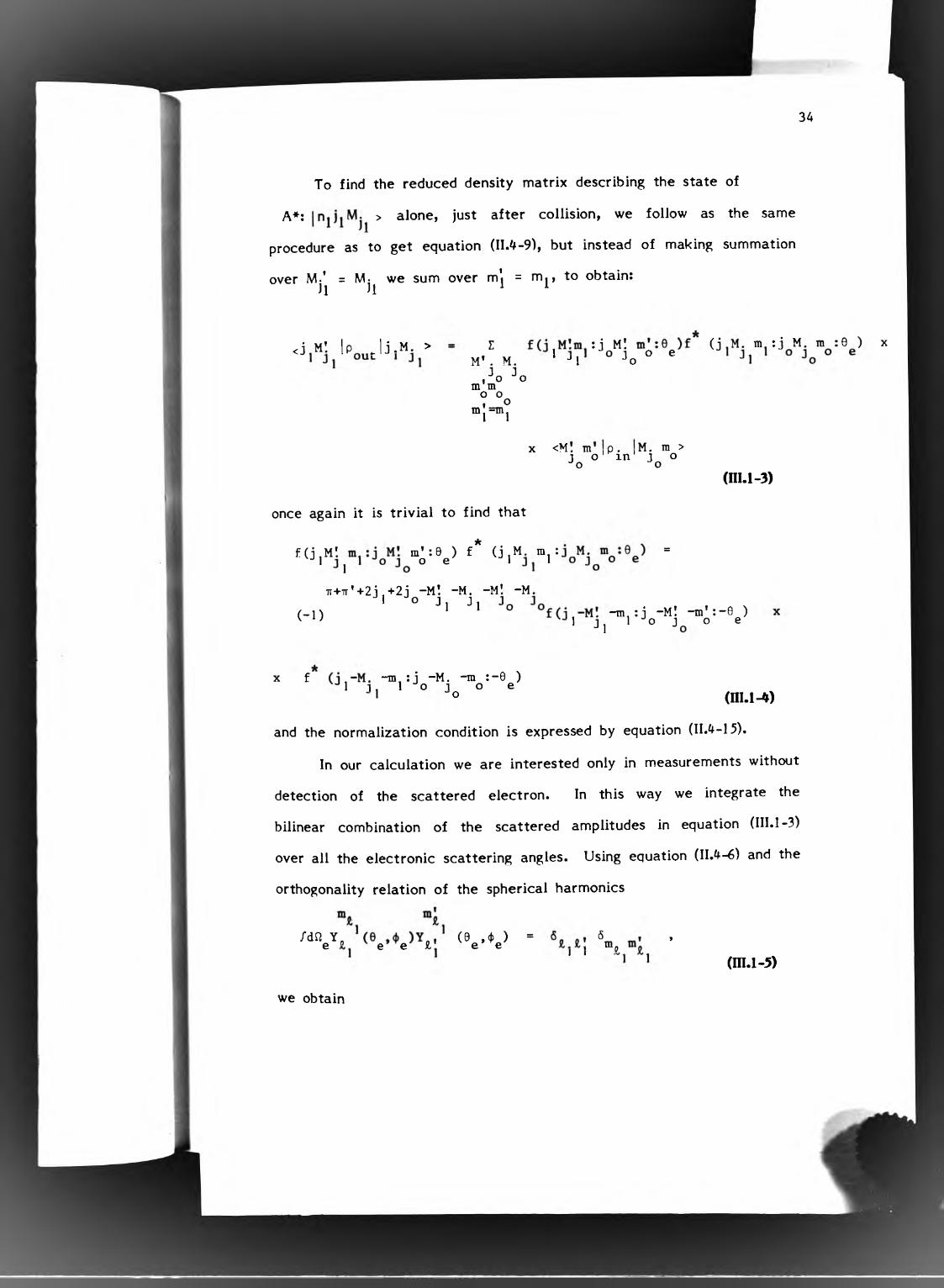
To find the reduced density matrix describing the state of

A*; > alone, just after collision, we follow as the same

procedure as to get equation (II.4-9), but instead of making summation

over M-’ = M, we sum over m', = m,, to obtain: ll ll ^

<j MÎ Ip J j .M . > I : j Ml ( j m : j M tn : 0 ) xM' . M.

.Jo Jomm0 o1 omi=mi

1 "o j o e •'I ‘’ o

X <M. m p . M. m > 1 o' in' J o • o o

(ni.1-3)

once again it is trivial to find that

£(jlM ; m;:e^) f * ( j ,M. m, : »1

TT+TT'+2j j+2j^-MÎ -M. -MÎ -M

( - 1 )o J, J,

° -m,: j -MÎ -m ': -0 )’ Jj 1 -"o J o e

X f -m,:j -M. -m :-0 )1 1, 1 o 1 o e

1 o (ni.1-4)

and the normalization condition is expressed by equation (II.4-15).

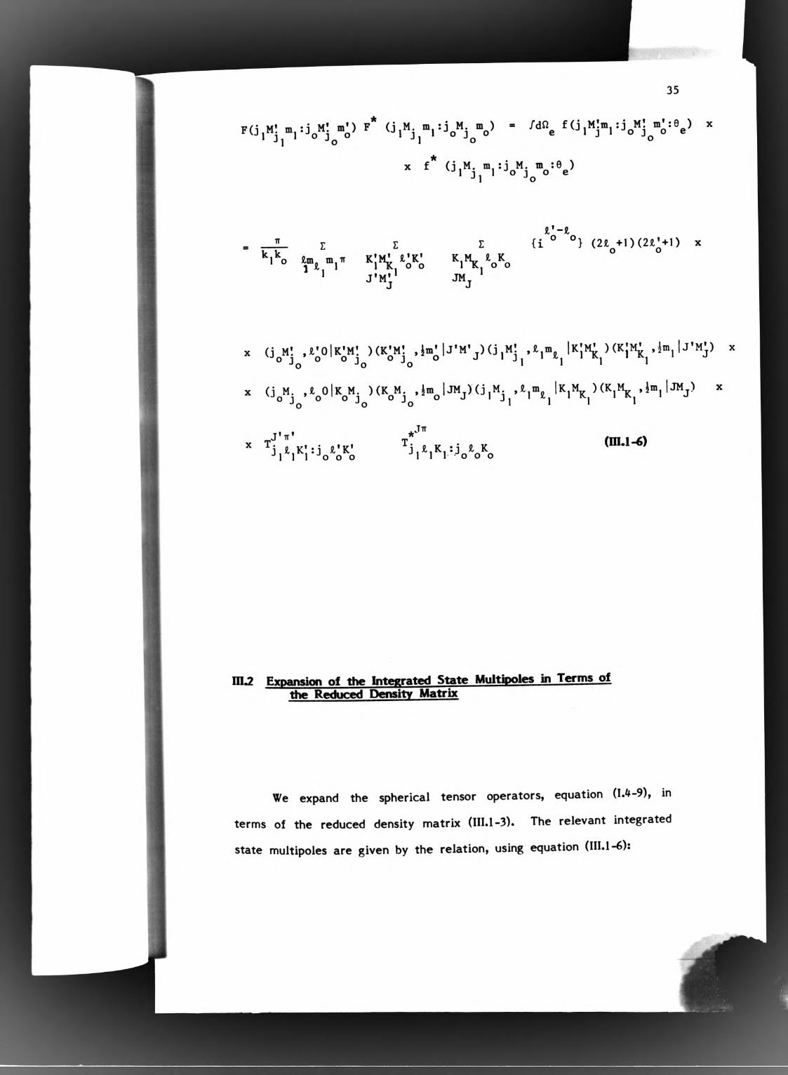
In our calculation we are interested only in measurements without

detection of the scattered electron. In this way we integrate the

bilinear combination of the scattered amplitudes in equation (III.1-3)

over all the electronic scattering angles. Using equation (II.4-6) and the

orthogonality relation of the spherical harmonics

J-dn.Y, ( 0 . . O • \ -1 Ie e e Í,’ ' e ' ' e

(m.1-5)

we obtain

36

> = (2K + 1)^ EMî M. m

'Ml M. m'm

Jo J o o° o

( - 1 ) 1 Jl (j.M! o -M, |KQ) > Jj ' Jj

X <m: V “ o> " (- ¡. « j " r ” j VJ Q Jq l o l U

(m ^ -1)

where we assume transitions between two well defined energy levels.

As we mentioned before the matrix < P in i ’ jo'^o ^

above equation contains all the dependence of the integrated state

multipoles on the initial polarization vectors of the colliding partners.

For instance the following physical situations may arise:

(i) For unpolarized initial beams the excitation processs is axially

symmetric around the z-axis (we choose z-axis as the direction of the

incoming beams). Applying the transformation operator D(0 0 y )^q and

making use of equation (1.^-7a), we have

then

> = 0 (n i.2-2)

Furthermore! according to reflection invariance in any plane through z-

axis we get in particular, using equation ( 1.^-6):

< Î(ii)îo> = 0

In this case the residual nonzero multipoles are the monopole

<0"(jj)Qo>un and the alignment parameter <^ (jp20^un*

(ii) If one of the polarization vectors of the incoming beams or

both of them has a component lies along z-axis, reflection invariance in

planes through the z-axis no more holds, this gives:

37

but the process is axially symmetric around the z-axis and as a

consequence equation (III.2-2) is still required.

(iii) In case of transversally polarized initial beams, one can

choose the direction of the polarization vector as y-axis and x-axis

perpendicular to y- and z- axes, the excitation process, described in

figure (2b), is invariant under reflection in the x-z plane and

consequently equation (1.^-6) holds. Because of summation of the

bilinear combination of the scattered amplitudes over all the electronic

scattering angles further restrictions^ should be imposed to reduce the

number of independent parameters. These restrictions can be noted

from equation (III.1-6) in the following.

The total angular momentum of the system is conserved during

the collision, which give for unpolarized initial beams:

♦ "V , * ""l = ^ io * ""o

Mj, + * '” 1 = ♦ ""o

(in.2-5)

As a consequence we obtain nonzero multipoles if the following

condition is satisfied

m ! = M,h n

combining equation (III.2-6) with equation (III.2-1) results in

0 = 0 (ni.2-6)

Therefore, we have

Q 0 or MÎ M. (m.2-7)

and

(m.2-S)

If the incident electrons are transversally polarized equation

(III.2-5) is replaced by

Mj, * tr%. * m, = Mj^ * m'o

+ mi = Mj^ + mo

38

then

M.' - M;h U

= m - m« = ±1o o —(m ^-10)

Inserting equationss (III.2-7), (III.2-8) and (III.2-10) into equation (1.^-6)

we end up with the four nonvanishing independent parameters

< *i,)S o > = <^<h>5o>un

We note that in case of transversally polarized initial target

atoms and unpolarized electrons the condition (III.2-10) is replaced by

M.' - M; = m J - M; , (ra^-15))l )1 Jo Jo

and we follow the same procedure as before to reduce the number of

independent multipoles according to the case under consideration.

Now we are in a position to expand the integrated state

multipoles in terms of the bilinear combination of the scattered

amplitudes.

ra.2A Excitation From the S^to the P| State

Case 1 Unpolarized Initial Beams

The only nonzero multipole is

<3'(i)^ > = 979 1 - 1^ oo un 2/2 . ' i'

(m^A-16)

where is the total cross section for the excitation of the

magnetic sublevel Mj^.

Case 2 Longitudinally Polarized Electrons and Unpolarized Target Atoms

Only two parameters are required, the monopole

- <^<!>00'un

and the orientation parameter

= 275" i

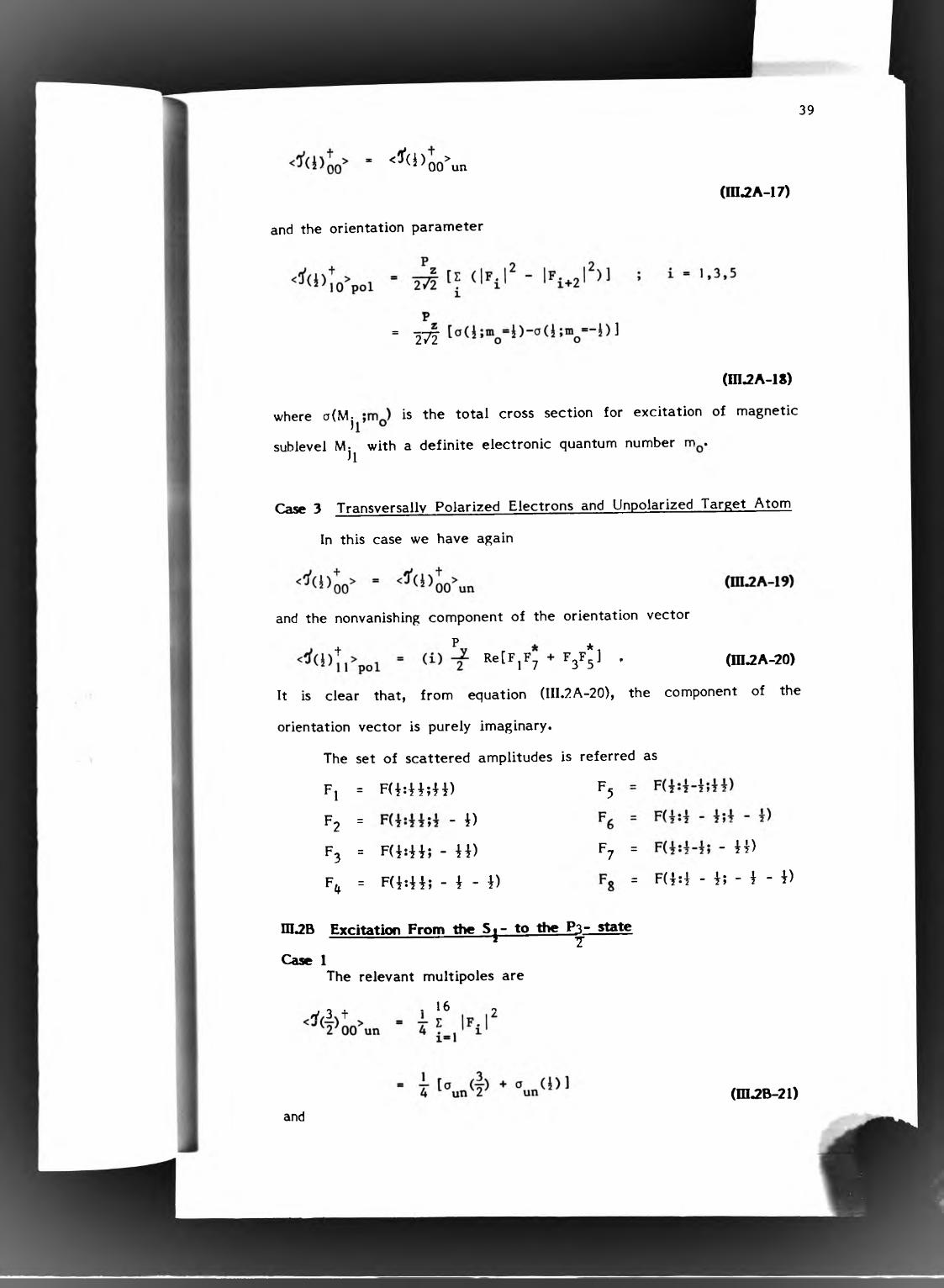
39

(in.2A-17)

(m ^A -is)

where a(M| is the total cross section for excitation of magnetic

sublevel M- with a definite electronic quantum number m .n

Case 3 Transversaliv Polarized Electrons and Unpolarized Target Atom

In this case we have again

and the nonvanishing component of the orientation vector

+ *Re[FjF^ + F3F3] . (ra^A-20)

It is clear that, from equation (III.2A-20), the component of the

orientation vector is purely imaginary.

The set of scattered amplitudes is referred as

Fi = F ( i :H ;H ) P5

F2 = - i )

F3 = F ( i :H ; - H )

F^ = F ( i : i i ; - i - i )

Fy = - H )

= F ( i : i - i ; - i - i )

ni.2B Excitation From the S t- to the P3- state------------------------------ i ^

Case 1The relevant multipoles are

^ 3 f .1 6 o

(m.2B-21)and

40

, 8 O 16 ,< ;/ (!)+> - X |F;1 ]^ T 2 Q un 4 £=i i=g ^

= T I®4 un 2 un

(in^B-22)

Case 2:

There are three independent parameters, defined as follows:

<^<l>20>unand

<^<l>Î0>pol 1

(in^B-23)

(in^B-2^)

= 4 ^ 1^) + (|f .| - I f . ^ j I ) ]

, i takes odd values only

,3= [3a(|;in^=i)+a(i;m^=D-3cJ(2;m^=“ n -o a ;m ^ = - i) ]

(m^B-25)

Case 3:In general we have four independent parameters

l>0 0 un< i (4 ) - >

2^20 un

(in^B-26)

(m^B-27)

(m^B-2S)and

‘ - 21 "" ' i’' W W W Î 6 '

Equation (III.2B-29) confirms that the alignment parameter,

<0 i)l)2i>poi» is a real quantity.

(in.2B-29)

41

The set of scattered amplitudes in this transition is written as

''l = F9 = F(|:44!44)>=2 = - i) FlO = f( |j44;4 - i)F3 = F(|:|è; - H ) Fll = F(|<44i - H )F* = F ( | | i i - i - i) Fi2 = F(|:44; - f - i)Fj = F f | : | - i ; i i ) Fi 3 = F(|^4 -Fé = F ( i | - 4 ii - 4) Fi 9 = F(|i4 - - i)Fy = F ( |: | - 4: - 44) Fi 5 = F(|:4 - i . _ H )Fg = F ( |: | - 4! - 4 - 4) Fié - f | : 4 - 1. _2 » i -

m3 Effect of Perturbations on the Decaying Process

The time evolution of an atomic states, where LS- or jj-coupling

holds during collision, under the influence of fine structure and

hyperfine structure interactions has been adequately considered

elsewhere.^»^^»^^»^^ But for the sake of completeness we briefly

consider the effect of perturbations in this section when the collision is

describable in jj-coupling scheme.

When LS-coupling does not hold during collision two somewhat

different situations may occur.

(i) Excited Atoms Violating LS-coupling

In this situation the spin-orbit interaction has an appreciable

effect during the collision, ie the collision time t^ is comparable with

the precession time of the fine structure states

E .f “E. (m 3-i)

The characteristic times is just the precession period of the spin

angular momentum and the orbital angular momentum vectors around

the total angular momentum of the excited atom.

As a result the scattered amplitudes and as will the integrated

42

state multipoles, being a function of the scattered amplitudes, referring

to different fine structure states are no longer correlated, but are

treated as independent parameters. Even in case of light emitted from

different fine structure levels is not resolved, the breakdown of LS-

coupling implies that the splittings, - E| , are large compared to

the level widths Y, ie the precession times of the fine strucutre states

are smaller than the atomic life time t = This result can be

understood by saying that many precessions will take place during the

atomic life time. Since we are interested in quantities averaged over

a time interval 0 -► tj (where is the resolution time and practically

we have t^ » t ) all interference terms with j| j| cancel each other

and only the time independent terms jj = jj will survive. Therefore

the radiation intensities from different fine structure levels add

incoherently and only interference of radiation from different hyperfine

structure levels need be considered.

We then have the density matrix of the excited atom just after

collision, t = 0, in the form (I is the nuclear spin):

p (0) = Pjj(O) X pj(0) (n i3 -2 )

(ii) Nonradiating Atom Violating LS-Coupling

In this case the total electronic spin is not a good quantum

number of the system. This arises when the target atom or any atom

formed in the collision violates LS-coupling, even though the radiating

atom obeys them. For instance, the Ly-a radiation resulting from

charge transfer of protons on Xe originates from the 2p-state of the

hydrogen atom, which obeys LS-coupling, however the states of Xe and

Xe'*’ do not.

In view of the above mentioned, three different situations may

occur:

(a) The transition operator T may depend explicitly upon the spin.

43

(b) The initial and final states of the collision partners, describing the

internal states of the collision partners before and after collision,

respectively, may not obey LS-coupling rules.

(c) The initial and final state vectors defined above may approximately

obey LS-coupling, but some of the substates of their multiplets may not

be energetically accessible.

In all the three cases the amplitudes of scattering and as well

as the reduced density matrix elements in - representation,

where i,M. refers to the state of the radiating atom, can still be 1 11

related to those in the - representation by a Clebsch-

Gordan transformation. As a consequence to spin-orbit interaction, the

scattering amplitudes referring to different states can interfere

yielding no reduction in the number of unknown parameters ensues from

the transformation to the - representation. Hence,

the scattering amplitudes describing the formation of the radiating atom

may be expressed in " representation.

Keeping in mind the above mentioned concepts, one can classify

the effect of fine and hyperfine structures on the decay process

according to the relation between the line widths and energy separations

of the relevant structure.

- Energy Separations and Line Widths are Comparable

Accordingly we have

T Tm T > Tj . j

and the scattered amplitudes referring to different fine structure levels

interfere. If also the fine structure splittings are large compared to

the hyperfine structure splittings, then

T « Tjij << Tjpip (ni.3-4)

and the excited ensemble decays before the hyperfine structure

44

interaction takes place.

The total density matrix, which only describes the excited orbital

states, just after collision, is then given by (no need to couple Pj(0)

under this circumstance):

p(0) = • (in.3-5)

Using equation (1.4-1) we obtain

P (0) =K Q. ■ ■ " J l ' j l J l 'J l

-'IAt time t the system is represented by a density matrix p(t) which has

evolved from the density matrix p (0) governed by the time evolution

operator U(t)

P (t) = U(t) p(0) U(t) (n ij-7 )

where,

U(t) = Exp (-iHt) , (ni3-8)

H = H + H' (ni3-9)o

and where the interaction term H' couples the spin and orbital states of

the system and is the unperturbed Hamiltonian.

Inserting equation (111.3-6) into equation (III.3-7) yields

P i l i ( t ) “ i Q. ’ Q,K, Q, i , J| J| J

J 1 J I

U(t)

(ni3 -io )

The integrated state multipoles describing the orbital states at

time t is defined as

<iJ'(jJj,;t)j^ Q > tr {p. Q. ^J, J,( i n j - i i )

Using equation (III.3-10) we get:

45

J i I » K. Q. Q-> <U(t)3'(j¡j,V Q.K. Q. JiJiX

X Q ^

(in.3-12)

q . (m.3-13)

where G ( j ' j ; t )^ l are the perturbation coefficients in this new1 1 K. KJj

multipole expansion.

Comparing; equations (III.3-12) and (III.3-13), we have

Qj Q

C.JQ. u ( t ) ' ' í ( j ¡ j , ; 0 Q )

(m.3-14)

Applying the Wigner-Eckart theorem, equation (1.3-4), and a

standard formulae^ of angular momentum theory for determination of

matrix elements of irreducible tensor operators with the help of the

symmetry properties of the Clebsch-Gordan coefficients, we obtain.

Q j Q

' e Ï % K Q3, ' ' J

IS. W. X1 1 (in j-15 )

where, “ E#| E* j j j j j j j

The Kronecker symbols in equation (I1I.3-15) indicate that

multipoles with different ranks and components can not be mixed, in

this case, by the interaction.

- Energy Separations are Large Compared to the Level Widths

Opposite to the previous case, interference between amplitudes

referring to different fine structure levies are not allowed. Therefore

the total density matrix describing the orbital states of the excited

system, just after collision, is given by equation (III.3-2).

Using equation (1.4-1), P(0) can be written in the form

P(0) - I X * 0>i^-’l K. X. * 0K.K- X. ' j , 3, 1 J| Jl(in.3-16)^

where X| are the components of the integrated state multipoles

> in the spin polarization frame (defined by taking the spinX.

polarization direction of the scattered atom, h , as a quantization axis)

and we assume that the nuclear spins of the excited ensemble are

polarized along the quantization axis.

Applying a similar procedure as in the previous case, we get

<0'(jj;t)i > = t v i o . X I)

46

Jj i J,

= tr {p. (t)i/(j ;t)Jj 1 K.. X-

1 J]

X tr {U(t)0'(jj)j^^ X t(I)^ QU(t) 0'(jj;t)} X l} (in j-1 7 )

' X. " KX; X

1

(in 3 -is )

where 2 is si unit operator in the spin space. Comparing equations

iIII.3-17) and (III.3-18) we obtain for the perturbation coefficientX. Xj j +I+F+K .

Z ( - 1) < t ( I ) > XKjFF’

(2F+1)(2F’ + 1)[(2K_+1)(2K. +l]^(K 0,K. X- Ikx. )K \ j fI J, 1 J| J, J] C l -M JK. K

x-{ I j, F'> EXP{-i(E^^j.,-E.^p)t-Y. t>

(n i3 -i9 )

where the symbols and are the

6j- and 9j- symbols, respectively.

Under the condition that atomic and nuclear spins are both polarized

along the same direction, tc , we replace Xj by Qj^.

The Clebsch-Gordan coefficient, 6j- and 9j- symbols, in equation

(III.3-19), put the necessary restrictions due to the angular momentum

47

coupling rules:0 < K “ K,. X* Í 1*

0 ;< Kj 21 Ik . - k^Ií Kí k . +k j , I ' j ,

These restrictions limit the number of possible perturbation coefficients

for each jj.

Now, if the splittings, Ej^pi - E|^p, are comparable with the line

widths, ie ^jpip - > interference between states of different hyperfine

structure levels (the time dependent terms in equation (III.3-19)) are

significant. For some physical situations it may happen that the

splittings are smaller than the line widths, then the oscillatory terms

with F' i F, in equation (III.3-19), average out during the comparatively

long life time and are neglected.

In the physical situation of interest where the nuclear spins are

initially unpolarized (Kj = 0) and the precession time t .p,p much

smaller than the life time t, equation (III.3-19) reduces to

21+1 I (2F+1)1

V ' " " Ì EXP i-Y t )

(m.3-20)

inj> Radiative Decay of an Excited Atom

The decaying process have been considered under the following

assumptions.

- The atoms have been instantaneously excited at time t = 0 and their

states are specified by a density operator p(0) which is assumed to be

known.

- The excited atomic ensemble is considered as a statistical mixture of

states 1 (here we suppress all quantum numbers which are

necessary to describe the state in addition to the angular momentum

quantum number, for sake of simplicity) which are assumed to be

degenerate in M. but not in jj.

48

- At a later time t the ensemble decays to lower levels |jMj> by

emitting photons.

- The excitation and decay processes do not change the atomic and

nuclear spins.

- The density matrix P (n^»t), which contains all information about the

system (atoms and emitted photons) at time t, is given by:

p(fi^,t) = U(t) p(0) U(t)' (m.4-1)

where the operator U(t) describes the time evolution under the influence

of the interaction between the excited ensemble and the

electromagnetic field, Vy(t), of the virtual photons.

In the first order perturbation theory this time evolution operator

is written as:

U (t) U(,(t) { l - i g/''dtUg(t)'^V^(t)UQ(t)} , (n u -2)where U (t) is the free time evolution operator corresponding to the

o

unperturbed Hamiltonian.

In view of these assumptions the elements of the polarization

density matrix of photons observed in the direction in the interval

0 t and in the photon detector frame are given byP(fi . t ) , , , = C M I <jM.|r .IjlM ! >< j:M .,lp (0 )| j M. > x

y \ A j A I J, I J, ' J|

iM.

X < j , M . ^ l 4 l j M . > X

j r-iCE ., -E. n - ) t 11-expL 1 J

i (E .,-E , ) + (y , i+Y. )

(III.4-3)4

where C(u)) = dfiy, c is the velocity of light in atomic units, d^^is 2-nc

the element of the solid angle into which photons are emitted.

The quantities £ and £ left-handed

circularly polarized light) are the spherical components of the dipole

vector £ in the "helicity-frame" spaned by the three basis vectors

V l * T -7 ( « , t A = ®0 n(m ^-4)

49

where e^, and ¿2 have polar angle (6y<i> ), (6^+90,4. ) and

(0 ,d>+90), respectively, in the collision system, figure ( 1).Y Y

L = ’'+1 ^+1 ’'-1 -1 ’'O YUsing equation (1.4-1), equation (III.4-3) becomes

P ( n ^ . t ) = C(o>) S <jM,lr .IjjM! x j j M ’Kai’.M; J * ' J| J| JlKqj,.

j|M. j « , ' J 1 J

l -E X P [- i (E . ,-E. ) t - H Y . i + Y . ) t ]___________ J]

i (E . , -E . ) + H Y i i+ Y . )Jj J, Ji Ji( I I I . 4-5)

= C(w) 1K q j j j ,

Kq

l -E X P [ - i (E . , -E . ) t - H Y . i + Y . ) t ]___________ J 1 J 1_______ 1

i ( E , , - E . ) + H Y ; .+ Y . )h Ji Ji h

( I I I . 4-6)

50

Comparing equation with equation we havetrir 'ffi* 1 ) rt) = <jM. Ir. , 1 j IMI > x

(ra^-7)

Applying the Wigner-Eckart theorem, equation (1.3-^), on equation

7) three times, and taking into account that £ is a tensor of rank one,

allows us to separate the geometrical parts (represented in the Clebsch-

Gordan coefficients) from the dynamical parts (represented in the

reduced matrix elements).

Hence t 1tr - I 3(-0JM.

X (jM.,j!-M! |l-X’)(jM.,j -M ll-X)(j!Ml ,j -M jKq) x J 1 Jj J * Jj * J] '(in.4-8)X <j 1 I r 1 1 j Jxj I 1 r I 1 j J>*

More simplification of equation (III.^-8) can be done by using the

relation

(c Y .a d f- * ) [ m ] =

X ~(2eV i) * *

then we obtain

tr {rj , (j;jj)r][} = 2 <j 1 1 1 H jj><j 11 r 1| jj>* (-1)

(11.4-9)

j+ jj+ X ’

X (1 -X M X | K -,)^ ]_ 1, j }

(in.4-10a)

In case of decay from a well defined energy level to the same final

state, we have

51

t r = l<j r I I j,>l (-1) '

f l I K'l(l-XM xlK-q)^ , . V] J J J

(nu-lOb)

Now by differentiating equation with respect to time,

one gets the reduced density matrix of those photons emitted at instant

t .

p ( S ^ , t ) = C(a.) £Kq r r 'Kq

where(ni.4-11)

E X P [ - i ( E j , - E j ) t - ! ( Y j . + Y . ) c l/nw-i2)

The exponential factor in equation describes the time evolution

of the excited states, between excitation and decay, whereas the

multipoles contain all information about the excitation

process.

It is more appropriate to transform the multipoles from the

photon detector frame to the collision frame using equation (I.^-7b)

+ - ............. t _ - - (K)

(in.4-13)

DCh '*' I<Q)gQ is the relevant transformation operator.

Substituting equation (IH.^-13) in equation (III.^^-ll), we have

(m.4-14)

Using equations (III.3-18) and (III.if-13) in equation (111. 1- 1 ), yields

P(ii , t ) . C M Z t r ( r x^ K. KqQ. ^

l - T K . Q. l - ' l ’ ^'K. K * ' '“y “O'n > D(fi. - KJ

1

where the trace is given by equation (Ill.ii^-lOa) and the perturbation

coefficients are given by equation (III.3.19).

52

In the special case of interest, where the energy separations are

iarge compared to the level widths and the atomic and nuclear spins

are unpolarized, equation reduces to

K=K.qQ'

_^wvj j »»-/jç. '■''Jl'K. Q.1 J, J,

where now the trace is given by equation (Ill.i^.lOb) and the perturbation

coefficients are given by equation (III.3-20).

ni.5 Stokes* Parameters Description of the Emitted Radiation

The integrated Stokes' parameters are calculated by comparing

equation (IH.^-16) with equation (1.2-6). Keeping in mind that, according

to our previous assumption the decaying process does not change the

spins of the excited atoms and consequently the dynamical factor

appearing in equation (Ill.^-lOb) does not change if it is calculated in

the LS- or jj-coupling scheme.

ni.5A The Decay Process P| —» S|

Case 1 Unpolarized Initial Beams

I - C(ai) |<0 II r II l>|^ ^ 3 (m jA -I )

(n , jA - 2)

Case 2 Longitudinally Polarized Initial Electrons and Unpolarized Target Atoms

Equation (III.5A-1) still holds, but we have for the circular

polarization

2r/2iMj - C(o.)|<0 ||r II l>|^[-Çcose^G,(i)<3’(!)^o % o l'

(nUA-3)

53

andiTij = In^ = 0

Case 3 Transversally polarized electrons and unpolarized target atoms

Again equation (III.5A-1) still survive whereas Iri2 now takes the

form

ITI2 = C(o))l<0 II r II l>|^[-|sin sin <t> Gj (i 111 pol

Cra.5A-5)

If one considers excitation by a steady flux of incoming electrons

the time at which the photons are emitted is no longer uniquely defined

with respect to the excitation time, and the time dependent exponential

in the perturbation coefficient, equation (III.3-20), may be integrated

from t = 0 to t = “ with negligible error. In case of caesium atom

we have,

G « ( i ) = — = X0 Y

Gj ( i ) = 0. 34375 T .

ID.5B The Decay Process Pq

Case 1:I - C(«)|<0 II r II l > r fi[<5o(f)<5'(|)oo'

. i (3 cos2e„-i)S ;(| )<a '(| )^^>^ jJ

= -c(o)) |<0 II £ I

(m.5B-6)

In,

Case 2:

IH2 = 0

1>|^[| sin^e G .(4 )<a'4 )^ >' 4 Y 2 2 2 20 un ( ¡ „ ^ b-T)

(m.5B-S)

The intensity I and n are given by equations (III.5B-6) and

(III.5B-7), respectively, but H2 is given by

55

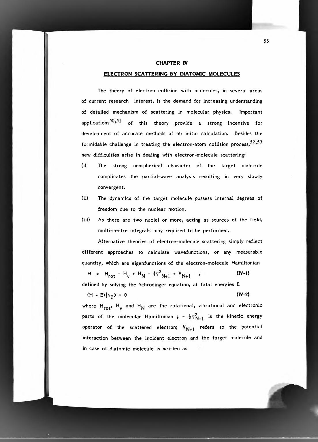
CHAPTER IV

ELECTRON SCATTERING BY DIATOMIC MOLECULES

The theory of electron collision with molecules, in several areas

of current research interest, is the demand for increasing understanding

of detailed mechanism of scattering in molecular physics. Important

applications^® of this theory provide a strong incentive for

development of accurate methods of ab initio calculation. Besides the

57 53formidable challenge in treating the electron-atom collision process, *

new difficulties arise in dealing with electron-molecule scattering:

(i) The strong nonspherical character of the target molecule

complicates the partial-wave analysis resulting in very slowly

convergent.

(ii) The dynamics of the target molecule possess internal degrees of

freedom due to the nuclear motion.

(iii) As there are two nuclei or more, acting as sources of the field,

multi-centre integrals may required to be performed.

Alternative theories of electron-molecule scattering simply reflect

different approaches to calculate wavefunctions, or any measurable

quantity, which are eigenfunctions of the electron-molecule Hamiltonian

H = H * + H + H., - I V., ,rot V N N+1 N+1 (IV-1)

defined by solving the Schrodinger equation, at total energies E

(H - E)|'1'£> = 0 (IV-2)

where H and H., are the rotational, vibrational and electronic

parts of the molecular Hamiltonian ; - is the kinetic energy

operator of the scattered electron; refers to the potential

interaction between the incident electron and the target molecule and

in case of diatomic molecule is written as

56

N+1i= i

'B

(IV-3)

where we assume a target molecule of N-electrons, r are their

coordinates and and Zg are the nuclear charges located at and

Similar to equation (11.3-6), the total wavefunction ^ is expanded

at each internuclear separation R as follows

f I V •k(IV-4)

where (i)j, in general, involves rotational, vibrational and electronic

states; describes the motion of the scattered electron and Cj are

N+1-electron antisymmetrized functions which allow for the

delocalization and correlation effects.

Because of the complications encountered in solving equation (IV-

2) we require taking advantage of any simplifying feature^^ that may

be available in each range of electron-molecule distances. For instance

at large distances the interaction is weak and nearly central and the

angular momenta of the electron and the molecule need not to be

coupled. At short distances, the total angular momentum JL and the

internuclear distance ^ couple strongly and A = I,. ^ is a well defined

quantum number. In such case the Body-Fixed frame of reference

(fixed with the molecule) is a natural choice to carry out calculation.

At some carefully chosen b o u n d a r y o n e transforms the solution

from the Body-Fixed frame to the LAB frame (in which the molecule is

rotating) and by introducing the nuclear Hamiltonian, continues the

solution of the resulting equations into the asymptotic region.

Hopefully one can find such transformation radius where all short range

interactions can be ignored in the outer region. The entire problem can

be solved in the BF frame under the following conditions:56>^7

57

The energy of the incident electron is very large compared to the

threshold energy.

- Strong long range interaction is not dominant.

- Nonresonant scattering.

We now sum up, very briefly, in the following sections some

important concepts which form the basis of the electron-molecule

scattering theory, limiting ourselves as much as possible to the scope of

the problem of interest.

IV.l Bom-Oppenheimer and Fixed-Nuclei Appraximations

The great disparity of electronic and nuclear masses allows one

to consider separately the motions of the electrons and the nuclei in a

molecule. So, in principle, the properties of the molecule could be

determined by calculating the electron motions for each possible

configuration of the nuclei, whose relative positions would enter these

calculations only as a parameter. This is the essence of the Born-

Oppenheimer approximation, therefore one can first solve the electronic

problem with the nuclei fixed. The nuclei are then assumed to move in

response to the adiabatic potential energy corresponding to the

stationary electronic state. However, corrections should be taken into

account for the breakdown of the Born-Oppenheimer approximation due

to the small electron velocities, large nuclear velocities or where two

or more electronic energy curves cross or come very close to one

another.

If the collision time is small compared with the characteristic

rotational and vibrational times, ie the incident electron passes the

potential area before any vibrational or rotational coupling takes place.

58

we need only consider the electronic Hamiltonian for the electron-

molecule system as the nuclei are then assumed to be fixed. This is

the Fixed-Nuclei approximation^^»^^ where any measurable quantity will

correspond to an average of all the possible molecular geometries over

the relevant molecular states.

IV.2 Representation of the Nuclear Motion (Rotation and Vibration)

As mentioned before the Born-Oppenheimer approximation enables

the electronic and nuclear motions in a molecule to be separated from

each other. The molecule persists in a particular electronic state with

a corresponding electronic energy during nuclear motion. The electronic

energy and the energy due to the electrostatic repulsion of the nuclei

both vary with the internuclear separation, and together provide the

potential that determines the rotational and vibrational motions.

Inclusion of rotational and vibrational motions obeys the following

classification:

If the collision time t^ is small compared with the characteristic

rotational times t .,. , 1E’ -Erot rot

one can find an orthogonal transformation^^»^^*^^ which connect the

two sets of wavefunctions and as well the T-matrices calculated in the

Body-Fixed (molecular rotation is neglected) and Laboratory (molecular

rotation is included) frames. Then, the relevant scattering amplitudes

and cross sections for transitions between rotational states can be

obtained.

For slow electron collision compared with the characteristic

rotational times.

E* ^-E ^rot rotthe rotational Hamiltonian can no longer be neglected and the Body-

59

Fixed frame treatment may be replaced by a Laboratory frame

treatment. However, a simplification of this treatment, given by Chang

and Fano,^^ showed that for slow electron colisions, the electron and

molecule interaction energy will still dominate the rotational

Hamiltonian for sufficiently small electron-molecule distances. The

Body-Fixed frame wavefunctions can be used in this internal region, and

then transformed at the boundary of this region (using a unitary

transformation). This procedure provides the boundary conditions for

the solution of the Laboratory frame equations in the outer region

including the rotational Hamiltonian.

Similarly if the collision time is small compared with

characteristic vibrational times.1

E ’ -E = Tv v

V V

.58an adiabatic transformation of the T-matrices can be applied, we

obtain

where A is the molecular symmetry; the integration of equation (IV.2-1)

is carried out over the nuclear coordinate corresponding to the initial

and final vibrational states X^,X^|.

A hybrid expansion^^»^® can be used if the time of collision is

not short compared with the characteristic vibrational times but is short

compared with the characteristic rotational times.

Finally if the collision time is large compared with both the

characteristic vibrational and rotational times

E ' -E v V

^ E ’ “EV V

an expansion in terms of the rotational and vibrational eigenfunctions

may be used. This increases the size of the system of equations and

thus tends to make its practical solution much more difficult.

However, this difficulty might not be great by using the simplification

60

of the frame transformation approach. Luckily we seldom meet this

type of situation, we then do not attempt this problem.

IV.3 Exchange and PolarizatriCTi Potentials

The scattering electron is indistinguishable from the molecular

electrons. Hence the system wavefunction must obey the Pauli

principle, ie 'I'g must be antisymmetric under interchange of any two

electrons. This requirement gives rise to exchange effects.

Combining equations (IV-1) and (IV-5) yields, after some

straightforward calculation,

2k2)u.^(r) = 2 Z (V, .+W,,)U,,.(r)

dr“ r “ j i j i j jk (IV.3-1)

where all correlation terms in equation (IV-5) are neglected, and ^.^(r)

is the set of radial parts of equation (IV-5), and where the direct

matrix elements are written as

(IV3-2)

and the exchange matrix elements, which interchange bound orbitals in

’ij ' I ''ij I

(|>j with continuum orbitals to the right of equation (IV.3-1), are

defined by

W..U.k(r) = - /dr K( i j|r ’ r )U .k (r ’ ) ,

K(ijlr’r)N

m»1 ij X

(IV.3-3)

ini')

X g , ( i jW ; A A )A m r » lA+l[max(r,r') ]'

(IV 3 -»)

where the target orbitals are expanded as

7 I ’'aaX m

(IVJ-5)

61

and g. are coefficients given by the product of four couplingA

coefficinets.

Solution of equation (IV.3-1) represents a formidable challenge,

therefore a number of approximate models to remove the nonlocality of

the exchange operator have been developed to treat the exchange term.

Such an operator is said to be 'nonlocal' (because it requires knowledge

of the integrand throughout space, rather than only at a single point).

Consequently, the exchange operator in equations (IV.3-1) and (IV.3-3) is

replaced by a simple local exchange potential energy function, ie

representing the electron-molecule static exchange by an approximate

local potential made up of static and exchange contributions. Recent

applications to treat exchange terms have been focused on either the

Free-Electron-Gas^^>^^»^^ (FEG) or the semiclassical^^ (SC) exchange

models.

Burke and Chandra^^ proposed a totally different approach to the

problems posed by exchange. This approach is based on the fact that

in the exact static exchange theory of electron scattering from a

closed-shell molecule, the radial scattering functions are necessarily

orthogonal to the bound orbitals of the target molecule. In a sense,

one can think of this condition as imposing constrains on the scattering

functions. These constrains are not the only effect of the exact

nonlocal exchange terms on the scattering functions, but Burke and

Chandra argued that they may be the most important ones. One can

derive the scattering equations of their procedure by starting in the

static approximation, in which exchange is completely neglected, and

then imposing suitable orthogonality constrains on the solutions of these

equations. This method of solution is called the orthogonalised static

method.

So far we did not include any correlation terms, in particular no

polarization of the target molecule due to the slow approach of the

62

incident electron to the bound electrons in the target is considered.

Electrostatic and exchange effects dominate the near-target region.

Further from the molecule, a new interaction that becomes important is

the induced polarization interaction. The adiabatic change in energy

felt by the field of the incident electron in the dipole approximation is

written asymptotically as

H l l~ ” 4

r ^ “ 2r (IV3 -«)V p (r )

In this equation, a(r) is the polarizability of the molecule which is a

measure for the molecular capability to distort in response to an

electric field directed along r. Equation (IV.3-6) breaks down if the

electron closely approaches the molecule and also the adiabatic picture

breaks down at high energies and near the nuclei.^^

To properly take account of non-adiabatic effects and deviations

from the simple asymptotic form (IV.3-6), a model potential has been

introduced. The form of this model polarization potential is

Vp(r) (IV.3-7)

where r^ is an adjustable parameter which is usually chosen to give the

best agreement with experiment.

IV.^ Methods of Solution of the Scattering Process

Many alternative techniques have been widely introduced to have

an approximate solution of equation (IV-2). In this section a very short

overview is presented on the approximations used in solving the

scattering process, a little more detailed survey is also presented on the

R-matrix method which is used in our calculation.^^

One approach which has been widely used (for details see refs

63

is to make a single-centre expansion of the scattered electron

wavefunction and the target orbitals. This common centre of expansion

is usually chosen as the centre of gravity of the molecule. This

approach is appropriate at large distances where the electron-molecule

interaction is weak and nearly central, but convergence problems do

arise for all molecules except the lightest ones due to the presence of

nuclear singularities. These nuclear singularities provide a strong

coupling of a large number of partial waves at short distances.

Due to the slow convergence, associated with the single-centre

expansion method, other techniques,^^’^ so called multi-centre

expansion methods, are introduced. In these methods the collision

wavefunction is written in terms of a multi-centre expansion using a set

of square integrable functions.jif. 75

One of these methods is the T-matrix method, * in which no

partitioning of configuration space into different regions is explicitly

involved.

Another method is the R-matrix expansion technique. Following

the frame transformation approach^^ the configuration space is

partikioDfJinto different regions, figure now a further partitioning^

into a core region r ^ a and a potential field region r ^ a^, is

appropriate. Under conditions such that the adiabatic nuclei

approximation is valid for rotation, vibration, or both, then the relevant

frame transformation radii can be taken to be infinite ie the frame

transformation reduces to a constant transformation. The power of the

R-matrix technique derives from the fact that in the inner region a

fixed-nuclei. Body frame calculation of the R-matrix is sufficinet

followed by a relatively straight forward integration of the scattering

equations in the outer region.

64

Briefly speaking (for details see ref in the internal region,

assuming an incident electron upon an N-electron target molecule, the

Schrodinger equation is written as

(H - E + Ljj) '{'e = H % (IV-»-l)

w h e r e i s expanded, using equations (IV-4) and (IV-5), in the form

H».k 1

J (IV.4-2)

where the unperturbed target wave functions are denoted by 4» j, the

spatial one-electron continuum orbitals are denoted by Fj, while C|- and

dji are coefficients to be determined by diagonalization procedure.

The surface projection operator ^ in equation (IV.4-1) is

77introduced

L.1 c (lV.ft-3)

to remove the non-hermitian components of H in the inner region and

also ensures that the wavefunctions (IV.4-2) satisfy the required

logarithmic boundary condition at the R-matrix surface.

Following a procedure similar to section (II.3), the R-matrix is

related to the radial wafunctions U- of the scattered electron, in

channel i, by the equationdU.

U. = E R. .[a - b.U. ]1 . 1 1 c dr j j r=aJ c (DfA-4)

in which a is the distance from the centre of mass of the diatomic c

molecule to the spherical R-matrix surface.

Therefore,

R.i j

J _ v Z w J i i(IVJ*-5)

where Yj.: is defined on the R-matrbc surface by

Y, . = «!>. 1 'I', >ki 1 ' k r«a (IV.*-6)

65

Given the R-matrix at r = and assuming the usual asymptotic

boundary conditions, the set of second order coupled differential

equations,

dr r 1 ^(v iA -r )

can be integrated in the outer region to determine the K-matrix for

each E. = k?/2, where j^,(r) is the local asymptotic potential

coupling the channels i and i'.

66

CHAPTER V

DISCUSSION AND NUMERICAL RESULTS

V.l Low-Energy Scattering of Electrons by Caesium Atoms^^»^^

The study of the low-energy scattering of electrons by caesium

37 38 78atoms has received much attention over the last ten years. ^ »

Recent advances in experimental techniques, together with the

development of powerful numerical methods, have further stimulated

work on this process. Not only can total and differential, elastic and

inelastic cross-sections be measured but the use of high-resolution

polarized electron beams enable observables such as spin polarization,

the asymmetry function and the Stokes’ parameters to be determined.

Advances in numerical methods which now allow the inclusion of

relativistic effects directly into the scattering equations have enabled

theoretical calculations of these observables to be made. A stringent

test of the theoretical model is therefore available. It is hoped that

these results will be helpful to the various experiments which are

currently in progress or under preparation in Munster^ and Stirling.

V.l A The Scattering Calculation

The dynamical calculations were performed using the relativistic

81R-matrix method first described by Scott and Burke and programmed

in ref. This method, as discussed in chapter II, augments the non-

relativistic electrostatic Hamiltonian with operators from the Breit-Pauli

Hamiltonian thereby enabling some relativistic effects to be included

into the scattering equations which describe the collision. Consequently

the method allows the various effects which are important in low-

energy electron scattering by heavy atoms to be accounted for. These

effects resulting from strong-channel coupling, electron exchange.

67

relativistic effects and the influence of resonances.

As in recent calculations^^ we use a model potential to

represent the closed-shell core of the target atom. In our model we

therefore assume that one valence electron and the colliding electron

are interacting with each other in the average field of the 5 core

electrons. The R-matrix basis functions used to expand the total

wavefunction are defined, using equation (II.3-1), as follows,

E c . . . $ . ( l ) u . . ( 2 ) + E d. 4).(1,2)K I J K 1 IJ j J K J (V.lA-1)

where the unknown coefficients c-| and djj were determined by

diagonalising the following model Hamiltonian,

2 ^ 2 2 C^**®*) 2 jH = - H + V ( r . ) - a Z — — E -

(V.IA-2)

« is the fine-structure constant, Z is the nuclear charge and V(r) is a

model potential representing the core electrons. This is defined as

a ,V ( r ) - V„ + - 4 [ l - E X P ( - | - ) ] ^ + - 4 [ l - E X P ( - | - ) !

" r* ""c r® ""c (V.IA-3)

Here Vj is a Hartree potential constructed from Thomas-Fermi Core

orbitals, is the static dipole polarizability of the core, while aq and

r^ are treated as adjustable parameters for each orbital angular

momentum. Values for these adjustable parameters were found by

calculating the negative eigen-energies of the following equation,

,2

a 10

(- + V(r) + k ) U(r) = 0dr

CV.1A-*)

The values of a and r were varied until the eigen-energies ofq c

equation (V.lA-4) gave energy splittings in good agreement with

experiment. The values used in the scattering calculation together

with the corresponding eigen-engergies are given in table 1.

We include the following five target eigenstates in expansion

(V.lA-1),

6p P. 3 (V.lA-5)

68

Each of these states was represented by a single configuration one-

electron function which, together with the core functions form the

Hartree potential, were calculated using the SUPERSTRUCTURE

program.

The R-matrix continuum orbitals were determined by imposing a

logarithmic derivative of zero at the R-matrix radius of 40.3555 a u.

This radius r_, was chosen automatically by the code to ensure that for

r ^r^ exchange between the incident electron and the target could be

neglected. These orbitals were orthogonalised to the core and valence

orbitals. Sixteen continuum orbitals were retained in the expansion for

each orbital angular momentum in order to guarantee convergence over

the energy range considered in these calculations.

All quadratically integrable correlation functions were included in

the expansion (V.lA-1) which could be constructed from the 6s, 6p and

5d orbitals with the appropriate symmetry as discussed in the next

secion. The diagonal elements of the Hamiltonian matrix were adjusted

so that the theoretical target energy splittings were in good agreement

with experiment.

K-matrices were calculated for each of the total angular

momentum from 3 = 0 to 10 for both even and odd parities. This

ensured that converged scattering amplitudes could be calculated over

the energy range from 0 to 3 eV. The inclusion of five target states

gave rise to up to 18 coupled channels.

V.IB Analysis of the resonamxs

In an earlier work a two-state (6s-6p) calculation was employed

which accounts for almost all the static dipole polarizability of the

ground state. They obtained a total cross section which was in

reasonable accord with experiment and the present calculation in energy

69

regions which were not close to the 6p and 5d excited-state thresholds.

However, inclusion of the 5d state in the present work introduces a

large number of additional resonances, particularly in the neighbourhood

of the 6p ^Pi ^ and 5d ^D3 ^ thresholds. Inclusion of this state is i i2 -p 2

therefore important if accurate results are to be obtained close to

these excited-state thresholds. These resonances have a pronounced

effect on the angular distributions and their number and complexity

explains the difficulty that Gehenn and Reichert experienced in

analysing their experimental measurement of these cross sections.

Most of the resonances are associated with the inclusion of the

quadratically integrable function in equation (V.lA-1). These allow

physically for the situation where the incident electron is captured into

a state whose lifetime is long compared with the collision time. We

included the following 35 quadraticaliy integrable functions:

6s2 Ice 0I ç c - s u 1 0 O e 9 1 i»

^0, 6s6p "^Po,l,2» P l» ^P ^ P n ,l,2 ’ ^P ^ 2 ’6p^ ^Sq> 6s5d 2 3> ^s5d 6p5d Pq j 2 >6p5d *P<j, 6p5d ^D®^2,3' '■ 2> ’

6p5d 5d^ ‘ S§, 5d ^Po,i,2,> *^2 ’ ’

5d ‘ g|.(V .IB-I)

Of course not all of these give rise to observable resonances.

For example, the 6s is not seen since its energy is below the

6s threshold and this corresponds to a bound state of Cs . Also

many of the others lie at too high an energy and are too broad to

noticeably affect the cross section.

A further class of resonance which we observe corresponds to the

situation where the incident electron is temporarily captured at very

large distances in the long-range field of the target in an excited state.

This is most likely in our calculation near the strongly polarizable

70

.0 2^e6p ^Pi 3 states of the target, since our inclusion of the 5d D 3,5 ^*2 2 2

states allows to account for most of the strong long-range polarization

potential in this case.

One of the most satisfactory ways of analysing and describing the

resonances is by reference to the eigenphase sums. It is well known85

that near an isolated resonance this quantity has the following behaviour

ir

(V.lB-2)-16(E) = 6q (E) + tan ^

where *q(E) is a slowly varying background phase shift and r and E . are

the width and position of the resonance, respectively. Hence the

phaseshift increases by tr rad in the neighbourhood of E . However, in

practice, particularly in a complex situation such as we are considering

in this discussion, this simple picture is often obscured. Firstly, the

rate of change of the background phaseshift can be as large or larger

than the resonance term itself, and can either be increasing, due to

attractive polarization potentials, or decreasing just above a threshold

involving a virtual or bound state. Secondly, several resonances with

different widths can be overlapping. Finally, strong configuration

interaction effects mean that identifying a resonance with a single

configuration in (V.lB-1) can only be an approximate description.

With these qualifications in mind, we present, in figures (5-1^),

the eigenphase sums for the resonant symmetries which from (V.lB-1)

are seen to be J = 0 to with odd and even parities. In an attempt

to assign a configuration to each resonance we performed a number of

additional calculations. We begin by calculating the eigenphases in LS-

coupling neglecting the relativistic terms in the Hamiltonian defined by

equation (V.lA-2). We carried out three such calculations, in the one-

state (6s), two-state (6s-6p) and three-state (6s-6p-5d) approximations.

This enabled us to observe how the resonances appeared and changed in

71

character as additional states and closed channels were added. The

three-state eigenphases together with the corresponding R-matrix poles

were analysed in detail. This allowed us to assign each reasonance with

a configuration. The five-state relativistic calculation was then

performed and we were able to observe how each LS-coupled resonance

was split by the spin-orbit interaction and distributed into different

total angular momentum symmetries. These assignments were confirmed

further by an analysis of the relativistic R-matrix poles.

In figures (5-1^) each resonance is designated by a letter. The

corresponding configurations are presented in table (2). The lowest-lying

odd parity resonance is located close to the threshold in 3 = 2

symmetry, figure (7). It clearly has the configuration 6p5d and can

also be seen at slightly higher energies in the 3 = 3 and 3 = ^

symmetries, figures (8,9). We find this resonance at a lower energy

37than Burke and Mitchell which is in good agreement with Gehenn and

78Reichert. This resonance is simply a consequence of the inclusion of

the 5d state in our calculations. It is the influence of this resonance

which is responsible for the broad 'bumb' just below the threshold

in the cross section shown in figure (15). Lying very close

to the threshold we find a narrow resonance to which we have

assigned the configuration 6pns ^p°. This is clearly seen in the 3 = 0,1

and 2 symmetries, figures (5-7). This resonance cannot be associated

with any of the quadratically integrable functions in (V.lB-1) so we

have concluded that it is the result of the capture of the incident

electron in the long-range potential field of Cs as discussed above.

Near the threshold a number of resonances are found. Below the

threshold there is a 6s6p ^p° and a 6p5d ^D2. In both these cases the

rapid increase in the eighenphase sum is cut short by the onset of the

^P3 threshold. Between the ^Ps and 3 thresholds we find a broad 7 7 7

72

6p5d resonance and a distinctive feature in the 3 = 0,1 and 2

symmetries, figures (5-7), which is attributable to the 6p5d

7 2configuration. Because of the near degeneracy of the ^03 and D52 2

thresholds resonance structure in this energy region are difficult toO Q

resolve. However, we believe there are indications of a 6p5d

resonance in the 3 = 1,2 and 3 symmetries, figures (6-8), close to these

thresholds.

We are turning our attention now to the even symmetries. Here

we only observe resonance structure in the 3 = 0,1,2 and 3 symmetries,

figures (10-13). The rise in the eigenphase sum above the threshold2in the 3 = symmetry, figure (1^), is probably due to the polarizability

of the 6p state which is accounted for by inclusion of the 5d state. In

the even symmetries the lowest-lying resonance occurs below 0.5 eV

where a broad feature with configuration 6s5d D is observed in the

3 = 1,2 and 3 symmetries, figures (11-13). Close to the threshold

in the 3 = 0 symmetry, figure (10), we find a distinctive resonance

which is the combined effect of two resonances, the 6p S and the

6p2 ^P®. The 6p ^P® is also observed above the ^P| threshold in the

3 = 1 and 2 symmetries, figures (11,12). As in the odd symmetry we

find evidence for the capture of the incident electron by the long-rangey

potential field of Cs. This time it occurs at the P^ threshold in the 3? — e

= 1,2 and 3 symmetries, figures (11-13), with configuration 6pnp D .

D7 1

2 2There are no indications of any resonances around the D3 and 'D 5

thresholds in the even symmetries, figures (10-1^).

Despite the large number of resonances identified from the

eigenphase sums only a few sharp features appear in the cross sections

for the transitions -»• ^P3 » figures (15-17). This is

because many of the resonances in different symmetries overlap in

energy and strongly interfere with each other in the total cross

sections.

73

V.IC Differential Cross section. Spin Polarization and Scattering Asymmetry

We described in section how to calculate differential cross

section, spin polarization and scattering asymmetry for a general

transition from an initial state Ijo^jQ^ final state . Here

we discuss our numerical calculation for these quantities.

In figures (18,19) we show the elastic differential cross section

a and the scattering asymmetry = Py for the three energies (0.816

eV, 1.632 eV, 2.0k eV). Absolute values of A^ up to 20% are found

near the minima in the elastic cross sections around 125°; the relation

of high absolute values of A^ to the minima in the cross sections is a

36well known feature in the elastic Mott scattering process.

In figures (20-25) we show the functions Py and A^ and the

differential cross sections for inelastic scattering (transitions

6s I ^ 6p ^Pi The first notable feature of the curves is the high t 2 »2

absolute values of P and A even for very small scattering angles (iey *

less than or equal to 20°); these high values are not necessarily

combined with minima in the cross sections. The second interesting

feature to be noted is the following approximate symmetry relation in

the formP (n == - 2P (4-)

Cv.ic-1)(V.lC-2)

where the arguments i and A indicate the final states P^ and P ^

respectively. Relations (V.lC-1) and (V.lC-2) are very well fulfilled for

2.0 eV and are a clear indication of the validity of the so-called 'fine-

structure' effect discussed by Hanne.^^ In this effect the spin-orbit

coupling within the target and the spin-orbit interaction of the

scattered electron are assumed to be weak and the spin-dependent

effects then arise from the transformation from LS-coupling to a

P y (! ) - 2 P / f)

A ^ (!) “ -2 A ^ (| )

74

representation determining transitions between fine-structure levels.

The only qualitative agreement for 1.632 eV is due to close vicinity of

resonances and thresholds, where Hanne's approximation cannot be

expected to be valid.

In figures (26-37) we present results for the differential cross

section and spin polarization of the scattered electrons as a function of

energy at eight scattering angles (10°, 30°, 50°, 70°, 90°, 110°, 130°,

150°). expressing these quantities as a function of energy at a fixed

angle involves a length calculation. Since there are as yet no

experimental results available to compare with we only used a small

number of energy points to give an indication of the structure involved.

These figures are only intended as a guide to experimentalists until

more data become available.

In figures (26-29) the differential cross section for unpolarized

initial beams is plotted as a function of the incident electron energy

for different scattering angles 0^. As expected dominant structures can

be seen in the resonance region, especially around the and

thresholds at 1.39 and 1.46 eV. Figures (30-33) show the spin

polarization Py of the scattered electrons, again for initially unpolarized

beams and for the transition -*■ It should be noted that, apart

from the resonance region, the absolute values of Py are rather small (

15%). In figures (34-37) we show the spin polarization Py of the

scattered electron beam when the electrons are initially fully

transversally polarized.

V.2 Stokes' Parameter for Inelastic Electron-Caesium Scattering44

In chapter III we described the polarization properties of light

detected from an excited atom. In view of that description the Stokes'

75

parameter of the light emitted in the decay 6p -► in

atomic caesium after electron impacat excitation are given by the

following:

Case A Incident electrons are initially transversallv polarized in the V- direction with polarization Py and photons detected in the Y-direction

(i) Cs : 6p

G o(!)<5 '(5 )^>n, = Hj - 0

(ii) Cs : 6p ^P3 6s 7

¡2 °2^2^ ____________n,

2 00 un 2 2 2^20 un

4/5 G,(|)^ ■ 4Gg (|) G, 4 ) < +„>2 '0 0 un 2 '“2 2 20 un

(V.2A-1)

(V.2A-2)

-34Go(|)<i/(|);o>un - S (|><^4>L^un

(V.2A-3)

(V.2A-4)

Case B Incident electrons are initially longitudinally polarized witiipolarization and photons detected in the forward direction

(i) Csg , ( ! ) < 5 ' ( ! ) Î o pol 0

(ii) Cs : 6p P3 7

/r =,<|x^<ik^

(V.2B-1)

(V.2B-2)

76

Before we discuss these coefficients we make the following

remarks:

(i) As can be shown by general symmetry arguments, j and

are proportional to the polarization component of the incoming

electrons, whereas (and the total intensity) is independent of the

electron polarization.

(ii) For the transition 6p 6s only ^2 different

from zero; nj and are proportional to integrated state multipoles

with rank K = 2, which cannot appear in an excited state with 3 = {

(in general 2j ^ K).

(iii) Integrated state multipoles with rank K = 3 which can appear3

in the description of an excited state with j = y cannot be measured in

this type of experiment.

It can be seen from the values of the perturbation coefficients,

written in section III.5, that the large nuclear spin I =-^ in Caesium

causes a significant depolarization of the emitted radiation. With

^2^7 = 0.219 a rough estimate has shown that for example values of

N3I or I’ i/Pyl greater than 20% seem to be very unlikely.

In figures (38-^1) we present our numerical results for the

integrated Stokes’ parameters nj, case of transversally

polarized incoming electrons. The polarization dependent components rij

and TI2 are normalised to an initial electron polarization of 100%. As

expected from the values of the perturbation coefficients, the absolute

values of the Stoks' parameters are rather small, and it should be noted

that the polarizations n j and n 21 which can be measured in an

experiment, become even smaller if Py is less than 100%.

Also in figure (^2) we show our numerical results compared with

the only available measurement.^^ In this case the incident electrons

were polarized with polarization vector along the z-axis and the photons

detected in the forward direction. This shows a fairly good agreement

of our calculation with experiment.

77

VJ Vibrational Inelastic Scattering of Electrons by N j

90 9 QIn previous papers by Chang * it was shown that, using the

frame transformation formulation of Chang and Fano,^^ the resonant

differential cross section, at intermediate energies, in electron

scattering from N2-moiecule is due to z: in symmetry with a dominant

f component. He admits also p component to take a place in the

former.CK 91

In our work, we used the same technique as Burke et al to

extract the transition matrix, which contains all information about the

scattering process, in the static exchange plus polarization2

approximation, SEP. We carried out calculation for symmetry and

90only contributions from p- and f-partial waves, as in Chang's paper,

were included.

According to these assumptions the differential cross section for

55 90 97excitation from a vibrational state Vj to state v is given by » »

3a(v. -> v_) 1I (2J+1)[9.(10,10|L0)‘

4ky L , j1

X ,I^+A9' v. 1 ;v.l '1 f.(30,30|L0)2 { s S l I i

+ 42.(10,10|L0)(30,301l 0) P ^ l 9 | ^!^]P^(cos 6)Cl 1 jj i ’ f

(V3-1)

where Pj^(cos 0) is the Legendre polynomial and M-matrix is defined, in

general, by the relation

M ( j ) i - l '+ A

X T (A)v.1 f

-------- ------T- OlA,£'-A|jO) X

(2j+l)^

CVJ-2)

i f I ' are the angular momentum of the incident and scattered electron

and A is the component of the angular momentum along the internuclear

78

axis.

The vibrational transition matrix in equation (V.3-2), in the

adiabatic approximation, may be written as ( a is appended to distinguish

different target eigenstates with the same A )

,(A)1 f

T-|— . <X (R)|e (c J ^ \ r ) (R)|x (R)>1+5.« V- ‘a Aa ai,’ ' v.AO f 1‘ a Ha

CVJ-3)

In the present calculation, eleven equally spaced values of R

define the mesh of the internuclear distances and a theoretical

vibrational wavefunctions, X^(R), are used where only the first four

vibrational levels are treated. In this two channels problem, C-matrix

has the form

/ cos 6 (R) sin 6 (R) \

- (R) - I I ’\ -s in S (R) cos 6 (R) J (V J -*)

where 6 (R) is the mixing parameter which relates p- and f- waves

contributions to the scattered amplitudes.

Before we make our discussion we mention the following remarks

on equation (V.3-1).

(i) The first term stands for p- wave contribution, the second for

f- wave, whereas the last term is a mixture of p- and f- waves.

(ii) All interference terms between p- and f- waves have been

cancelled as a result of summation over all rotational states allowed by

the symmetry relations.

(iii) From the symmetry relations of the Clebsch-Gordan

coefficients, summation runs over even values of L. So, the Legendre

polynomial contains only even powers of cos 0 and we get an angular

distribution which is always symmetric around 90°.

(iv) The integrated cross sections are obtained by integrating

79

equation (V.3-1) over all the electronic scattering angles.

In figures (<f3a-^3d) we show the variation of the individual

eigenphases with the internuclear distance, at four incident electron

energies. It is clear that the p-wave eigenphase changes minimally as a

function of R as compared with the change of the f-wave eigenphase,

confirming that the f-partial wave dominates the resonance. Also, it is

shown the region where there is a strong mixing between p- and f-

partial waves at each incident electron energy. This is again

manifested on figures (^^a-^^d) where the mixing parameter is plotted

as a function of R at fixed values of energy. The rapid variation of BOQ

with R contradicts the assumption made by Chang® that is the

mixing parameter can be taken to be independent of the energy and the

internuclear distance.

Table (3) gives the integrated cross sections for V| = 0 v = 1,2

transitions, compared with other theoretical calculations and

experimental data. In general the calculations are in reasonable accord

with each other.

We present in figures (^5-47) our numerical calculations for the

vibrational excitation, Vj = 0 ■> = 1, angular distribution at incident

energies 20, 25 and 30 eV. Some other theoretical calculation and

experimental data are included for comparison. The circuled curves are

taken from Chang,^® equation (3) with a fixed B = 60°, after

93normalization to the experimental data of Tanaka et al at 20, 25 and

30 eV by multiplying by 7.8 x 10"^^, .1 x 10"^^ and 1.6 x 10

(cm^/sr), respectively.

Our calculation, of angular distribution, exhibits a minimum at

^0°, followed by a local maximum at 61° and another deeper minimum

at 90°. The present calculation shows, in general, a fairly good

agreement with Onda and Truhlar^^ calculation. At incident electron

80

energy 20 eV, the present calculation is agreeable with measurements

by Tanaka et al^^ and Pavlovic et al^® in shape but not in magnitude.

At 25 eV a good agreement is shown with Tanaka et ar^ data, whereas

there is a disagreement with the data of Pavlovic et al^® (this

disagreement is explained by Chang^^ as the resolution, in Pavlovic et

al^® experiment, was high enough to resolve the rotational states). At

30 eV our calculation is again agreeable with measurements by Tanaka

et al^^ and Truhlar et aP"' in shape but not in magnitude..95 ..

81

REFERENCES

Fano U (1957): Rev Mod Phys, 29 7if.

Messiah A (1965): Quantum Mechanics (North Holland, Amsterdam).

Blum K (1981): Density Matrix Theory and Applications (Plenum Press, New York and London).

McMaster W (195^): Am 3 Phys, 22 357.

Born M and Wolf E (1970): Principles of Optics (Pergamon Press, New York).

Fano U and Racah G (1959): Irreducible Tensorial Sets (Academie Press INC, New York).

Fano U (1953): Phys Rev, 90 577.

Blum K and Kleinpoppen H (1979): Phys Rep, ^ 203.

Bartschat K, Blum K, Hanne G F and Kessler 3 (1981): 3 Phys B: At Mol Phys, JH 3761.

Sommerfeld A (1916): Ann Phys (Leipzig) C 3, 21

Dirac P A M (1928): Proc Roy Soc, Ser, A 117 610.

Dirac P A M (1930): The Principles of Quantum Mechanics (OxfordUniversity Press).

Breit G (1929): Phys Rev, 21 553.

Breit G (1930): Phys Rev, 36 383.

Breit G (1932): Phys Rev, 39 616.

Doyle H T (1969): Adv Atom Mol Phys, 2 537.

Grant I P (1970): Adv Phys, 19 7WJ,

Armstrong 3r L and Feneuille S (197^): Adv Atom Mol Phys, 2

Armstrong 3r L (1971): Theory of the Hyper fine Structure of Free Atoms (3ohn Wiley &: Sons, New York).

Walker D W (197if): 3 Phys B: At Mol Phys, 7 97.

Chang 3 3 (1975): 3 Phys B: At Mol Phys, 8 2327.

Glass R and Hibbert A (1976): Comp Phys Commun, 125.

Hibbert A (1979): 3 Phys B: At Mol Phys, U L661.

Scott N S, Bartschat K, Burke P G, Nagy O and Eissner W B (198^): 3 Phys B: At Mol Phys, J7 3755.

82

25. Scott N S, Bartschat K, Burke P G, Eissner W B and Nagy O (198^): J Phys B: At Mol Phys, J7 L 191.

26. Burke P G and Robb W D (1975): Adv Atom Mol Phys, JJ_ 1^5.

27. Glass R and Hibbert A (1978): Comp Phys Commun, 19.

28. Burke P G and Seaton M 3 (1971): Meth Comp Phys, 1.

29. Hibbert A (1975): Comp Phys Commun, 2

30. Burke P G and Schey H M (1962): Phys Rev, 126 1^7.

31. Norcross D W and Seaton M 3 (1969): 3 Phys B: At Mol Phys, 2 ,731.

32. Mott N F (1929): Proc Roy Soc (London), A12^ ^25.

33. Massey H S W and Mohr C B O (19ifl): Proc Roy Soc (London), A177 3^1.

Farago P S (1971): Rep Prog Phys, 5k 1055.

35. Kleinpoppen H (1971): Phys, Rev, A3 2015.

36. Kessler 3 (1976): Polarized Electrons (Springer, Berlin).

37. Burke P G and Mitchell 3 F B (1973): 3 Phys B: At Mol Phys, 6 L161.

38. Burke P G and Mitchell 3 F B (197^): 3 Phys B: Atom Mol Phys, 7_2U .

39. Scott N S (1980): Ph D Thesis (The Queens Univ of Belfast).

UO. Taylor 3 R (1972): Scattering Theory (3ohn Wiley, New York)

^1. Percival I C and Seaton M 3 (1957): Philos Trans Roy Soc, A251 113.

U2. Fano U and Macek 3 (1973): Rev Mod Phys, 22 553.

U3. Khalid S M and Kleinpoppen H (198^): 3 Phys B: At Mol Phys, 17 2^3.

4^. Nagy O, Bartschat K, Blum K, Burk P G and Scott N S (198^): 3 Phys B: At Mol Phys, _17 L527.

U5. Bartschat K, Scott N S, Blum K and Burke P G (198 ): 3 Phys B: At Moi Phys, 17 269.

^6. Macek 3 and 3aecks D H (1971): Phys Rev, A2 2288.

U7. Blum K (1978): in Progress in Atomic Spectroscopy (edt: Hanle W and Kleinpoppen H, Plénum Press, New York and London) p 71.

^8. Brink D M and Satchler G R (1968): Angular Momentum (clarendon Press, Oxford).

83

66.

67,

King G W (1965): Spectroscopy and Molecular Structure (Holt, Rinehart and Winston, INC, New York).

Pavlovic Z, Boness M 3 W, Herzenberg A and Schulz G T (1972): Phys Rev, 676.

Tronc M, Azria R and Coat Y L (1980): 3 Phys B: At Mol Phys, 13 2327.

Mott N F and Massey H S W (1965): The Theory of Atomic Collisions (3 rd edition. Clarendon, Oxford).

Burke P G (1977): X ICPEAC, Electronic and Atomic Collisions. Invited Papers and Progress Reports (edt: Watel G, North Holland, Amsterdam) P201.

Chang E S and Fano U (1972): Phys Rev, 173.

Burke P G (1979): Adv Atom Mol Phys, 15 ^71.

Chang E S and Temkin A (1969): Phys Rev Lett, 22 399.

Lane N F (1980): Rev Mod Phys, 52 29.

Chase D M (1956): Phys Rev, m 838.

Chandra N and Temkin A (1976a): Phys Rev, A13 188.

Chandra N and Temkin A (1976b): Phys Rev, A l^ 507.

Hara S (1967): 3 Phys Soc jpn, 22 710.

Riley M E and Truhlar D G (1975): 3 Chem Phys, 63 2182.

Baille P and Darewych 3 W (1977): 3 Chem Phys, 67_ 3399.

Burke P G and Chandra N (1972): 3 Phys B: At Mol Phys, 2. 1696.

Nagy O, Burke P G and Noble C 3 (1985): to be published in 3Phys B: At Mol Phys.

Buckley B D and Burke P G (1977): 3 Phys B: At Mol Phys, 10 725.

Raseev G, Giusti-Suzor A and Lefebvre-Brion H (1978): 3 Phys B: At Mol Phys, JJL 2735.

Morrison M A, Lane N F and Collins L A (1977): Phys Rev, A15 2186.

Morrison M A (1979): Electron-Molecule and Photon-Molecule Collisions (edt: Rescigno T N, McKoy V and Schneider B I, Plenum Press, New York and London).

Collins L A, Robb W D and Morrison M A (1980): Phys Rev, A21 488.

Collins L A, Robb W D and Morrison M A (1978): 3 Phys B: At Mol Phys, Ü L777.

84

72. Temkin A (1966): Autoionization (edt: Temkin A, Mono Book Corporation, Baltimori^^

73. Hazi A U and Taylor H S (1970): Phys Rev, Al_ 1109.

74. Rescigno T N, McCurdy C W and McKoy V (1974a): Chem Phys Lett, 27 401.

75. Rescigno T N, McCurdy C W and McKoy V (1974b): Phys Rev, AlO 2240.

76. Burke P G; McChey 1 and Shimamura I (1977): 3 Phys B: At Mol Phys, 2 2497.

77. Bloch C (1957): Nucl Phys, 4 503.

78. Gehenn W and Reichert E (1977): 3 Phys B: A t Mol Phys, 25. 3105.

79. Hanne G F (1984): Private Communiction.

80. Kleinpoppen H (1985): Private Communication.

81. Scott N S and Burke P G (1980): 3 Phys B: A t Mol Phys, 4299.

82. Scott N S and Taylor K T (1982): Comp Phys Commun, 25 347.

83. Scott N S, Burke P G and Bartschat K (1983): 3 Phys B: At Mol Phys, i i L 361.

84. Eissner W, 3ones M and Nussbaummer H (1974): Comp Phys Commun, Z 270.

85. Nesbet R K (1980): Variational Methods in Electron-Atom Scattering Theory (Plenum Press, New York).

86. Hanne G F (1983): Phys Rep, 21 95.

87. Measurements by Nass P (1985): Institut fur Physik, Mainz, Germany (Private Communication).

88. Moore C E (1970): Atomic Energy Levels NSRDS-NBS3 (Washington, D C: US Govt Printing Office).

89. Chang E S (1977): Phys Rev, ^ 1841.

90. Chang E S (1983): Phys Rev, 709.

91. Burke P G, Noble C 3 and Salvini S (1983): 3 Phys B: At Mol Phys, l i LI 13.

92. Salvini S and Thompson D G (1981): Comp Phys Commun, 22 49.

93. Tanaka H, Yamamoto T and Okada T (1981): J Phys B: At Mol Phys, 14 2081.

94. Onda K and Truhlar D G (1980): 3 Chem Phys, 72. 5249.

85

95. Truhlar D G, Brandt M A, Srivastava S K, Trajmar S and Chutjian A (1977): 3 Chem Phys, 66 655.

96. Onda K and Truhlar D G (1979): 3 Chem Phys, 71 5107.

97. Rumble 3 R, Truhlar D G and Morrison M A (1981): 3 Phys B: At Mol Phys, L301.

98. Dehmer 3 L, Siegel 3, Welch 3 and Dill D (1980): Phys Rev, A21101.

TABLE AND FIGURE CAPTIONS

Table 1

Table 2

Table 3

Figure 1

Figure 2

Figure 3

Figure ^

Figures 5-9

Figures 10-1<

Adjustable parameters used in the model potential defined

in equation (V.lA-3). For i > 3 the values for i = 3

were used. Also shown are the corresponding

eigenenergies of equation (V.lA-4). The experimental

energies are taken from Moore^^.

Definition of the configuration assignments used in figures

5-lif.

Integrated cross sections (a^) for electron-N2 scattering in

v(0 1,2) vibrational excitation at several impact

energies.

Collision and detector frames.

Reflection in the scattering plane.

Precession of L and S about the axis of a diatomic

molecule.

Partitioning of space according to the frame

transformation theory^^.

The odd parity eigenphase sums for the symmetries J = 0,

1, 2, 3 and in e" + Cs scattering. The ^Pj>

and thresholds are indicated by arrows at 1.39, 1.^6,

1.80 and 1.81 eV, respectively.

The even parity eigenphase sums for the symmetries 3 =

0, 1,2, 3 and U in e‘ + Cs scattering. The ^P j» P_3 ,

^D3 and ^Ds thresholds are indicated by arrows at 1.39,2 2

1. 6, 1.80 and 1.81 eV, respectively.

Figure 15 Total cross section for the -► 25^ transition in Cs.

The ^P^> ^^5 thresholds at 1.39, 1.^6, 1.80J J T . .

and 1.81 eV, respectively, are indicated by arrows.

Figure 16

Figure 17

Figure 18

Figure 19

Figure 7.0

Figure 21

Figure 22

Figure 23

Figure

Figure 25

Figure 26-29

Figures 30-33

Figures 3íf-37

Figure 38

The same as fig 15 for -*■ transition.

The same as fig 15 for ^Si transition.2

Differential cross sections, 0(6^), for the transition

at the energies 0.816 eV(-.-), 1.632 eV(— ) and

2 M eV(— ).

Scattering asymmetry, Agie^) = Pyieg), for the transition

at the energies 0.816 eV(-i(-), 1.632 eV(-o-) and

2 m eV(-0*).

Spin polarization, Py(0e) and the asymmetry function

As(e e) ior fhe transition ^S j ->■ ^P| at energy 1.632 eV,

Py(0e)(-o-) and

As fig 20 at the energy 2.0^ eV.

As fig 20 for the transition ^S^-»^P3.

As fig 21 for the transition2

Differntial cross section, cr( 0 ), for the transition —>

^Pj at the energies 1.632 eV(-#-) and 2.0^ eV(-o-).

The same as fig 2 for the transition ^Si ^P2.*2The differential cross section for the transition ^S| -»■

in Cs, at the scattering angle ñ ^ = 10°, 30°, 50°, 70°,

90°, 110°, 130° and 150°.

The polarization vector, Pyi^e)» of th® scattered electrons

for the transition ^S^ ^S| in Cs at the scattering angle

©e = 10°, 30°, 50°, 70°, 90°, 110°, 130° and 150°. The

incident electron beam was initially unpolarized.

The polarization vector, Py(0g), of the scattered electrons

for the transition -► 2sj in Cs at the scattering angle

0 0= 10°, 30°, 50°, 70°, 90°, 110°, 130° and 150°. The

incident beam was initially fully transversally polarized.

Stokes' parameter ’ l/p for the transition P3 **■ ^5^ in

Figure 39

Figure UO

Figure 1

Figure ^2 7 7Stokes' parameter transition ^ S, ir

Figures ^3a-^3d

Figures

Figure ^5

Figure U6

Figure WJ

Cs as a function of the Collision energy. The arrows

mark the excitation thresholds ^P l, ^P3, and at7 2 2

1.39, 1.^6, 1.80 and 1.81 eV, respectively. The incident

electrons were initially fully transversally polarized in the

y-direction.

As fig 38 for n^/Py .

As fig 38 for 13.

Stokes' parameter n2/Py for the transition 2si in

Cs. Further details as in figure 38.

■?- in

Cs. The incident electrons were initally fully

longitudinally polarized in the z-direction.

SEP p- and f- wave eigenphases as a function of the

internuclear distance at incident electron energies;

a - 20 eV b - 25 eV

c - 27.21 eV d - 30 eV

As figs ^3a-^3d for the mixing parameter.

SEP differential cross sections in 10"f^(cm^/Sr) for vj =

0 v f = 1 transition at incident electron energy

20 eV.— , present calculations; — , Onda and Truhlar^^;

— —, Pavlovic et al^®; 0-0-0 > Tanaka et al^^; 000,

Changé®.

As fig ^5 at energy 25 eV.

As fig at energy 30 eV.#^^, Truhlar et al^^.

TABLE 1

**d Eigenenergy(Ryds)

Experimental energy (Ryds)

1 = 0 15.0 6U.0 0.9

6s -0.286723 -0.286^^82

7s -0.117355 -0.117578

8s -0.06if6^0 -0.06í^7í^6

i = 1 15.0 38.3 0.9

6p -0.181068 -0.181262

7p -0.08680^ -0.086922

8p -0.03^097 -0.03^^126

1 - 2 15.0 3t^A 0.9

5d -0.153620 -0.153789

6d -0.080163 -0.0806 ^6

7d -0,0U87U5 -0.0^9025

TABLE 2

A 6P ns \ , 1 , 2

B 6p 5d ^Di 2,3

C 6s 6p ^Pj

D 6p 5d

E 6p 5d ^D2

F 6p 5d

G 6p 5d ^Dj 2,3

H 6p2 ISq

I Po,l,2

3 6s 5d ^Di ,2,3

K 6p ^D i 2,3

Px =-P

la)

Figure 5

E igenphase sum (rad)N) Oi

Figure 6

Eigenphase sum (rad)

Figure 7

KJ

Elgenphase sum ( r a d )O) OD

Figure 8

Eigenphase sum (rad )

Figure 9

E igen p h ase sum (rad)Ui

Figure 10

Eigenphase sum (rad)

Figure 11

Eigenphase sum (rad)

ro N)

Figure 12

Eigenphase sum (rad) u) cr

Figure 13

E igenphase sum (rad) u) cn

m

Figure 14

E igenphase sum (rad)<jj Ol

Figure 15

Cross-section(TTa - )

Figure 16

Figure 17

2Cross-section ( ‘fToQ)

m

Figure 18

Figure 19

Figure 20

Figure 21

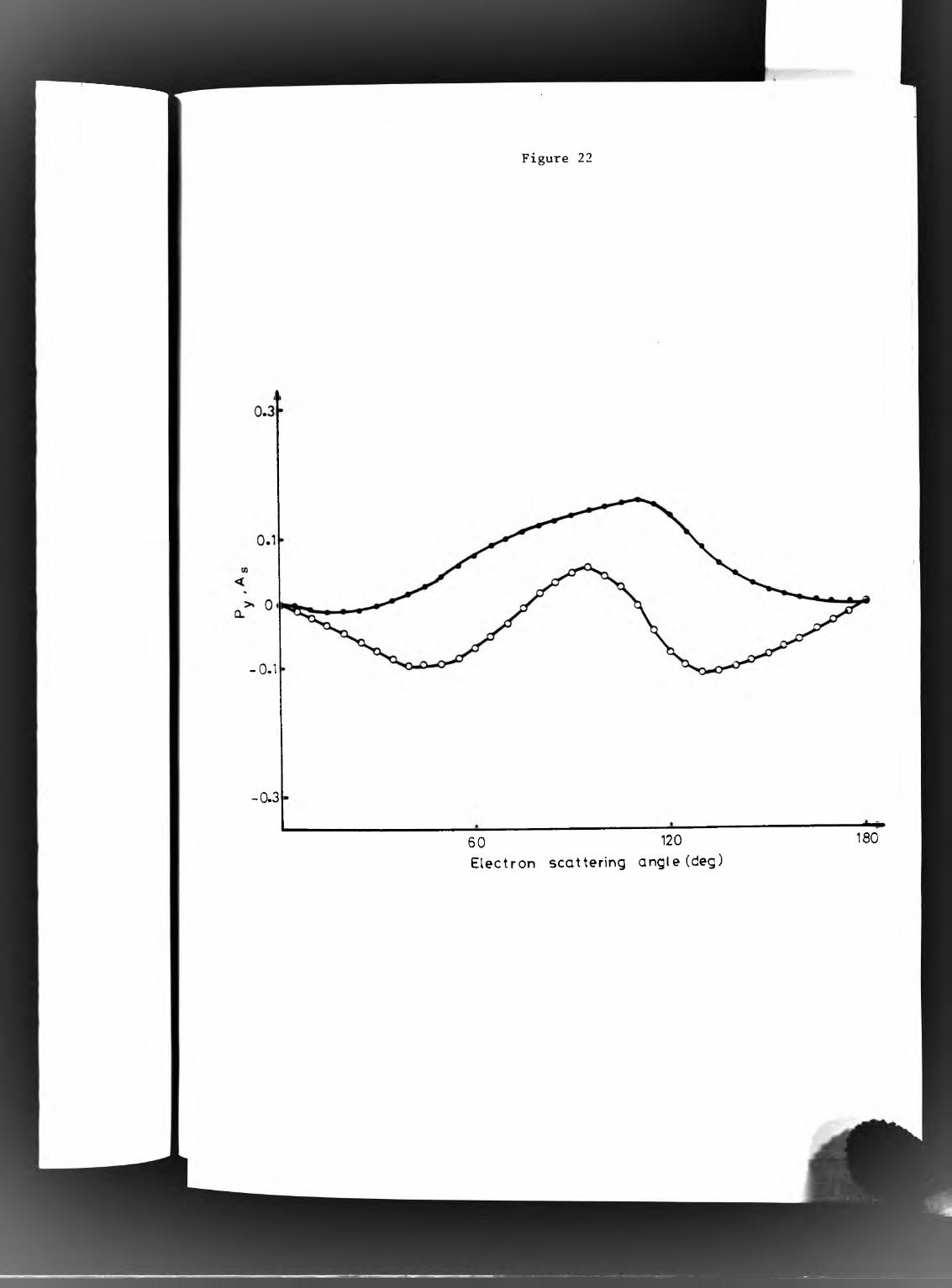
Figure 22

0

-0.1

-0-3

60 120 Electron scattering angle (deg)

180

Figure 23

Figure 24

Figure 25

Figure 26

2A00

2000

1600

1200

CO 800

800

600

400

200

1.0 1.5Electron energy (ev)

Figure 27

Figure 29

Figure 30

Figure 33

Figure 34

Figure 35

Figure 36

Figure 37

<D3(t>

(O

tn

CJl

m<t)

oi

tn

CD ro

Figure 38

Figure 39

Electron energy (ev)

0.12

Figure 40

0.08

CO

0.04

01.7 1.9

Electron energy (ev)

Figure 41

0

-0.04

- 0.12

- 0.20

1.9Electron energy (ev)

Figure 42

m<0

m

Figure A3

Eigenphases (rad)

Figure 44

Internuclear Distance (a u)

Figure 45

Figure 46

Figure 47

N>

W

(D