acknowledgements - unesco | building … sukara (president of the mab national committee) and at...

i

ACKNOWLEDGEMENTS

This research is funded by UNESCO/MAB Young Scientist Award grant number

SC/EES/AP/565.19, particularly from the Austrian MAB Committee as part of the

International Year of Biodiversity. I would like to extend my deepest gratitude to the Man

and Biosphere-LIPI (Lembaga Ilmu Pengetahuan Indonesia) which was led by Prof.

Endang Sukara (President of the MAB National Committee) and at present is substituted

by Prof. Dr. Bambang Prasetya, Dr. Yohanes Purwanto (MAB National Committee) for

endorsing this research, and Sri Handayani, S.Si. (MAB National Staff), also especially to

the Mount Gede Pangrango National Park for allowing to work at Selabintana and Cisarua

Resort, and the Carbon team members: Ahmad Jaeni, Dimas Ardiyanto, Eko Susanto,

Mukhlis Soleh, Pak Rustandi and Pak Upah. Dr. Didik Widyatmoko, M.Sc., the director of

Cibodas Botanic Garden for his encouragement and constructive remarks, Wiguna

Rahman, S.P., Zaenal Mutaqien, S.Si. and Indriani Ekasari, M.P. my best colleagues for

their discussions. Prof. Kurniatun Hairiah and Subekti Rahayu, M.Si. of World

Agroforestry Center, M. Imam Surya, M.Si. of Scoula Superiore Sant’ Anna Italy also

Utami Dyah Syafitri, M.Si. of Universiteit Antwerpen Belgium for intensive discussion,

Mahendra Primajati, S.Si. of the Burung Indonesia for assisting with the map and

Dr. Endah Sulistyawati of School of Life Sciences and Technology - Institut Teknologi

Bandung for the great passion and inspiration.

ii

TABLE OF CONTENTS

Page

LIST OF TABLES iii

LIST OF FIGURES iv

EXECUTIVE SUMMARY vi

1.0 INTRODUCTION 1

1.1 Objectives 3

2.0 METHODS 4

2.1 Study site 4

2.2 Measurement of carbon stock and estimating the biomass 6

2.3 Plant diversity 8

2.4 Relationship between carbon stock and plant diversity 9

2.5 Carbon value 9

2.6 Ecosystem service 9

3.0 RESULTS AND DISCUSSION 10

3.1 Estimation carbon stock and biomass 10

3.2 Plant diversity as the carbon stock performance and its conservation value

15

3.3 Relationship between carbon stock and plant diversity 32

3.4 Carbon stock and plant diversity as basis of an ecosystem services model

41

4.0 CONCLUSION

44

REFERENCES 45

APPENDICES 49

iii

LIST OF TABLES

Page

Table 1. Average carbon stocks for various biomes 1

Table 2. The main ecological zone of Mount Gede Pangrango National Park 4

Table 3. Allometric models used to convert measures of vegetation to AGB 6

Table 4. The average carbon stock in observation plot at 3 zones of MGPNP 11

Table 5. The average contribution of carbon stock from trees on 4 allometric equations

13

Table 6. Ecological index of 30 species with highest importance value on study site

16

Table 7. Class and category of tree density 18

Table 8. Relative value of ecological index component on Mount Gede Pangrango National Park

22

Table 9. Carbon stock, ecology indexes and formation at the subalpine zone 32

Table 10. Carbon stock, ecology indexes and formation at the montane zone 34

Table 11. Carbon stock, ecology indexes and formation at the submontane zone

35

Table 12. Bray-Curtis Index 36

Table 13. Highest ten species in carbon stock value on 4 allometric equations

37

Table 14. The approach of interval value test for carbon stock on the model of cubic polynomial regression

40

Table 15. Estimation of carbon stock on the nature forest MGPNP

41

iv

LIST OF FIGURES

Page

Figure 1. An egg of well-being 3

Figure 2. Study site map on Mount Gede Pangrango National Park 5

Figure 3. Sampling plot for carbon measurement made with length direction in line with elevation line with the assumption representing vegetation gradation on each elevation

6

Figure 4. Estimation of carbon stock and biomass on several elevations, AGB is aboveground biomass that consist of trees, understorey, litter and necromass

10

Figure 5. The value of trees proximity based on the elevation zone. 11

Figure 6. Carbon stock is stored in two classes of tree sizes on different elevations

12

Figure 7. Contribution of tree component, understorey, litter and necromass for carbon stock on different elevations

14

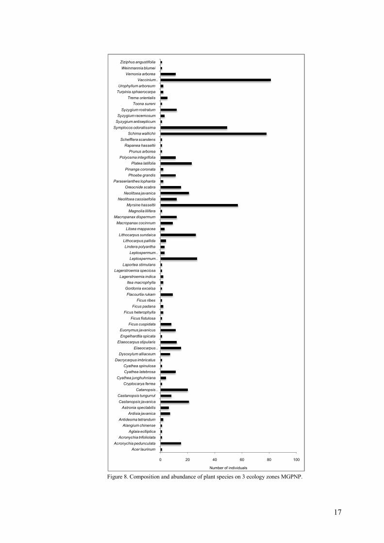
Figure 8. Composition and abundance of plant species on 3 ecology zones MGPNP

17

Figure 9. The relationship between species density rank and its abundance 18

Figure 10. Composition and abundance of plant species on subalpine zone 19

Figure 11. Composition and abundance of plant species on montane zone MGPNP

20

Figure 12. Composition and abundance of plant species on submontane zone of MGPNP

21

Figure 13. The relationship of basal area, density and importance value to carbon stock on the elevation of 2802 m asl

23


24


25


26

v

Page


27


28


29

Figure 20. The relationship between basal area, density and importance value to carbon stock on the elevation of 1271 m asl

30

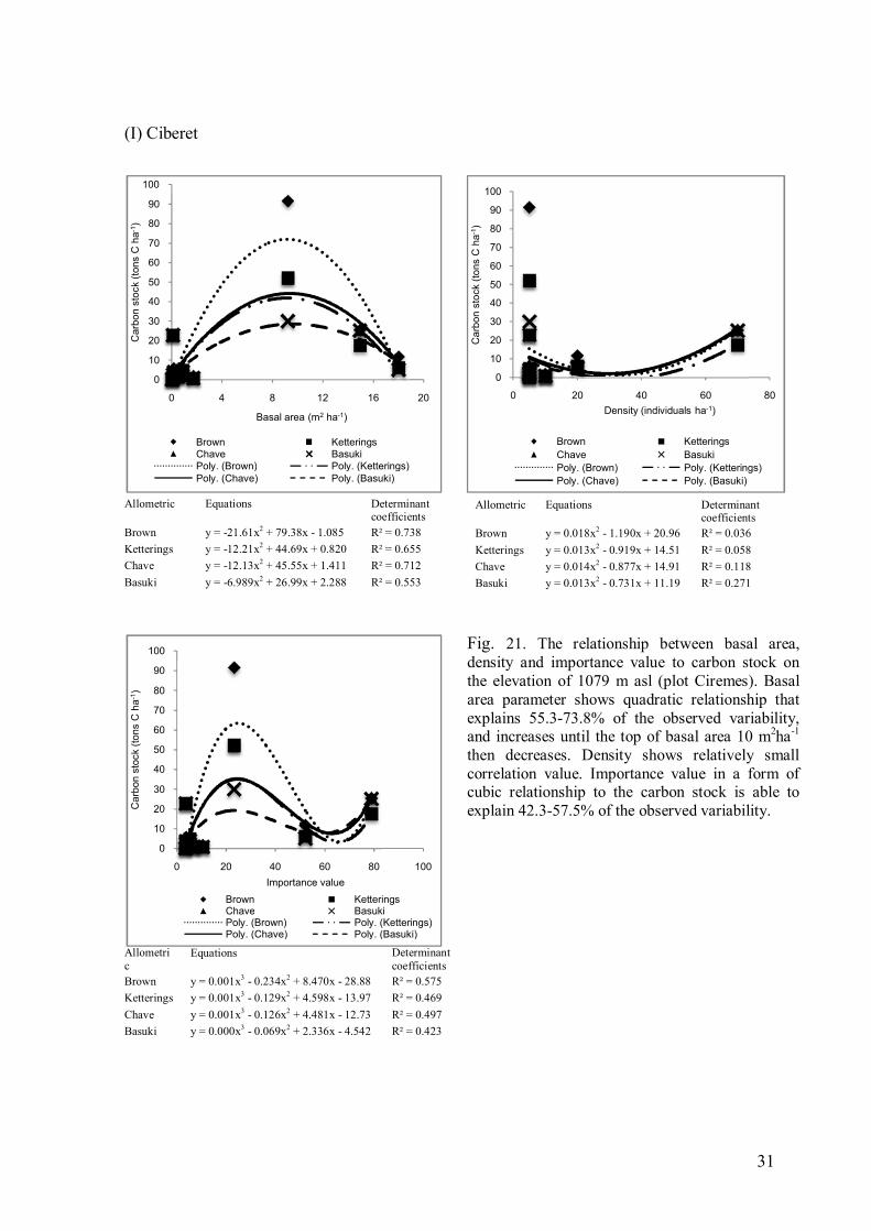
Figure 21. The relationship between basal area, density and importance value to carbon stock on the elevation of 1079 m asl

31

Figure 22. Carbon stock of plant species at the observation plot on Mount Gede Pangrango National Park

38

Figure 23. Model of cubic polynomial regression for correlation between Shannon Index and carbon stock on 4 allometric equations

39

Figure 24. Ecosystem services model on Mount Gede Pangrango National Park based on carbon stock and plant diversity

42

vi

EXECUTIVE SUMMARY

Mount Gede Pangrango National Park (MGPNP) is a wet-climate mount ecosystem

that is rich for its plant diversity and has a significant contribution in storing carbon stock

in its biomass and in time, it should be an ecosystem service. The purpose of this research

is (1) to obtain information and data of carbon stock in relation to the plant diversity on

nature forest ecosystem of Mount Gede Pangrango National Park as the core zone of

Cibodas Biosphere Reserve (2) to formulate ecosystem services model on the wet climate

mountains in West Java based on the strong linkage between carbon stock and plant

diversity, and (3) to support scientific data in welcoming REDD/REDD plus, thus the

result will directly contribute to the multistakeholder in Cibodas Biosphere Reserve for

participating in reserving the main site. The method of measurement consists of

(1) dividing Mount Gede Pangrango National Park in its each unique ecosystem

as follows: (a) submontane zone (1000-1500 m asl), (b) montane zone (1500-2400 m asl),

and (c) subalpine zone (2400-3019 m asl); (2) measuring the carbon stock above and

below ground by using World Agroforestry Center (2007) as a guide; (3) estimating the

biomass of branched trees by applying the equation of Dry Weight/DW as follows:

(a) DW = 0,118 D2,53(Brown, 1997), (b) DW = 0,11 ρ D2,62 (Ketterings et al., 2001),

(c) AGB est= ρ x exp(-1,499 + 2,148ln(D) + 0,207(ln(D))2-0,0281(ln(D))3) (Chave et al.,

2005), (d) Ln (TAGB) = c + αln(DBH) (Basuki et al., 2009). The estimation of the

biomass of non-branched trees uses DW = π ρ HD2/40 (Hairiah et al., 2001);

(4) calculating plant diversity by using quantitative parameter, including index of

importance value, index of diversity and index of similarity; (5) analyzing the relationship

between carbon stock and plant diversity by using excel program on Mac OS X Version

10.5.8 and model test of polynomial regression on the confidence level of 95%; and

(6) calculating of carbon value based on the ecological zone ability in supporting carbon.

The average result of carbon stock measurement (aboveground carbon stock) on 9

sites using four allometric equations in tons C per hectare is 399.717 (Brown/Br), 354.648

(Ketterings/Kt), 449.688 (Chave/Cv) and 325.724 (Basuki/Bs). The estimated biomass is

assumed that its 46% is stored carbon stock which is as much as 868.950 (Br), 770.974

(Kt), 977.583 (Cv) and 708.095 (Bs). The highest carbon stock is found on 2329 m asl

(montane zone), except Bs allometric on 2601 m asl (subalpine zone), and the lowest one

is found on 1355 m asl (Br) and 1079 m asl (Kt, Cv, Bs). The average of highest carbon

stock based on zone is on the subalpine zone, that is 409.751 (Kt), 553.858 (Cv),

vii

411.661(Bs) except Br (463.466) on the montane zone. It is presumably caused by

contribution of Vaccinium varingiaefolium, which is multistem as well as dominant species

on the subalpine zone. The maximum proximity value from the big trees to the small ones

happens on the subalpine zone, that is 280 individuals ha-1 of the big tree (2601 m asl) and

2950 individuals ha-1 (2802 m asl). Meanwhile the approximate average of contribution on

the aboveground carbon stock from the big trees 42.697-51.963% and from the small trees

29.664-35.892%. The tree component has the significant average contribution value to the

total carbon stock, that is 82.803% (Br), 80.692% (Kt), 84.994% (Cv) and 79.766% (Bs). It

shows the role of tree biomass is highly essential in supporting carbon. On the other side,

the average contribution on the aboveground carbon stock from understorey is as much as

1.302% (Br), 1.517% (Kt), 1.198% (Cv) and 1.559% (Bs); from litter is 12.895% (Br),

14.83% (Kt), 11.778% (Cv) and 15.735% (Bs); and from necromass is 3.308% (Br),

3.932% (Kt), 3.156% (Cv) and 4.117% (Bs).

It is known that there are 13 top species with the highest carbon stock

approximately between 60.159-772.624 tons C ha-1, those are Schima wallichii, Vaccinium

varingiaefolium, Castanopsis tungurrut, Lithocarpus sundaicus, Leptospermum flavescens,

Platea latifolia, Myrsine hasseltii, Toona sureni, Symplocos odoratissima, Neolitsea

cassiaefolia, Castanopsis javanica and Cyathea junghuhniana. The high value of carbon

stock on this research is a reflection of species dominance from all elevations which

carbon stock is measured.

It is an interesting fact that Schima wallichii is found from 1271 (submontane) until

2601 m asl (subalpine) which is shown with a high frequency of 0.778 and importance

value of 36.865. This is why eventually Schima wallichii has the highest carbon stock

value. Meanwhile, the crater species, Vaccinium varingiaefolium has the highest

importance value 49.152 with the width of basal area 314.714 m2 ha-1, even though with

small frequency of 0.222. Furthermore, it is important to note that this crater plot has the

lowest Shannon index, which is 1.409. Based on tree proximity class per hectare, it shows

that its 68.182% is classified into class occasionally (0-50), and its 25.76% is classified

into class often (51-150) and the rest is class abundant (100-450) that has relatively small

proportion, that is 6.06%. On subalpine zone, there are abundant of species on wet-climate

mountains such as Vaccinium varingiaefolium, Symplocos odoratissima, Myrsine hasseltii,

and Leptospermum flavescens. Montane zone is the widest area than two other zones and

there are species with the highest number in the area, such as Schima wallichii,

viii

Lithocarpus sundaicus, Platea latifolia, Neolitsea javanica and Elaeocarpus angustifolius.

The highest number on the submontane zone are Schima wallichii, Castanopsis tungurrut,

Oriocnide scabra, Castanopsis javanica and Phoebe grandis. The highest number of

species is often found at Selabintana V (1710 m asl) that is 25, then Pasir Ipis (1355 m asl)

that is 23, thus, both of them have relatively higher Shannon Index than other elevations,

which are 2.925 and 2.701.

Generally, all zones have similar tendency, which is they have positive and

significant correlation between ecology indexes (basal area, density, importance value) to

the carbon stock. The different ability in storing carbon at each zone is presumably related

to the level of tree proximity per hectare and number of species, because in time it will

affect the ecology indexes value. Tree proximity value per hectare accordingly from

subalpine to submontane is 93, 38 and 17; meanwhile the number of species is 16, 70 and

44. On the subalpine zone, the correlation value (R2) is found to be very high. The average

is 0.971 on basal area parameter and 0.991 on the importance value; meanwhile the

average for density is 0.768. These values are higher than the ones on the montane and

submontane zone. According to Bray-Curtis, based on the community composition, the

index of both elevation points on the subalpine zone has a same value as much as 79.8%

and it can provide the approximate average value of the total of with this sort of formation,

which is 409.751-553.858 tons C ha-1. Montane zone has 0.809 for the average of

correlation value on the basal area parameter, 0.764 for importance value and 0.571 for

density, and those values are seem lower than the ones on the subalpine zone. On the

Bray-Curtis Index, it is known that approximately 58-72% of species composition is

different and this formation can produce the approximate of total value of carbon stock

between 362.261-506.695 tons C ha-1. Subalpine zone has a lack of average of correlation

(R2) which is 0.474 on the basal area parameter, it is sufficient on the importance value as

much as 0.734 and those values are lower than the ones on the subalpine and montane

zone, except for density 0.586. Based on the Bray-Curtis Index, about 56-97% of species

composition is different and this formation can produce the average of total value of

carbon stock between 219.735-304.252 tons C ha-1.

The ability of carbon stock MGPNP in million tons C is on the montane zone with

maximum value of 6.463 (Br), 5.549 (Kt), 7.066 (Cv) and 5.052 (Bs), meanwhile the

minimum value on the subalpine zone is 0.507 (Br), 0.483 (Kt), 0.652 (Cv) and 0.485 (Bs).

Based on the conservation value aspect, special attention is needed for species that

ix

includes into IUCN red list, some of them are Euonymus javanicus, Dysoxylum alliaceum,

Engelhardtia spicata, Macropanax concinnus and Prunus arborea.

The relationship between Shannon Index and carbon stock is modeled in cubic

polynomial regression equation, because of the non-linear data spread pattern. However,

this model results on the relatively small correlation value (R2 = 0.236-0.284). The results

of the equation are y = 686.5x3 - 4349x2 + 8854x – 5375 (Brown), y = 542.2x3 - 3335x2 +

6543x – 3730 (Ketterings), y = 694.8x3 - 4287x2 + 8448x - 4852 (Chave) and y = 434.9x3 -

2668x2 + 5233x - 2950 (Basuki). The model using interval confidence of 95% and carbon

stock value on particular Shannon Index are in the interval of lower mean and upper mean.

Further research is required in order to reveal the relation between both of these variables

so that the appropriate model development is obtained.

The approach of ecosystem services model based on carbon stock and plant

diversity can be a foundation for structuring strategy of Low Carbon Development. It is

eventually aimed for the welfare of local people at Cibodas Biosphere Reserve which will

give a global outcome.

1.0 INTRODUCTION

One of the nature forests that become the core zone of Cibodas Biosphere Reserve is

Mount Gede Pangrango National Park (MGPNP). It has been the world-admitted

(UNESCO) reserve site since 1977. This site is a demonstration of sustainable development

referred to a global and important agenda such as Convention on Climate Change,

Convention on Biological Diversity, Agenda 21 and Global Strategy for Plant Conservation.

Plant diversity on this site has a significant contribution in storing carbon stock in its

biomass and in time, it should be an ecosystem service. Ecosystem services are an

instrument that is capable not only to provide local advantages, but also to maintain global

ecosystem. Conservation of forest biodiversity is fundamental to sustaining forests and

people in a world that is adapting to climate change. Strongly focusing on forests as the key

to managing the world’s carbon stocks—while disregarding the important role of

biodiversity in building forest resilience (UNEP, 2011). The location of MGPNP in

Sundaland is included into Global Biodiversity Hotspots (Conservation International, 2010)

as the category of an area of high carbon sequestration (180-959 tons per hectare) (UNEP-

WCMC, 2008). It becomes the reason that this area is one of the important, national and

global agendas to conduct biodiversity conservation including plant diversity and carbon

conservation.

Moist tropical forests are important for carbon sequestration, because they typically

have high carbon content (Table 1) and about half of the carbon in moist tropical forests

contains the vegetation, a higher percentage and a much higher quantity than in any other

biome (Gorte, 2009).

Table 1. Average carbon stocks for various biomes (in tons per acre) Biome Plants Soil Total

Tropical forests Temperate forests Boreal forests Tundra Croplands Tropical savannas Temp. grasslands Desert/semi desert Wetlands Weighted Average

54 25 29 3 1 13 3 1 19 14

55 43 153 57 36 52 105 19 287 59

109 68 182 60 37 65 108 20 306 73

Source: Adapted from Intergovernmental Panel on Climate Change, “Table 1: Global carbon stocks invegetation and carbon pools down to a depth of 1 m [meter],” Summary for Policymakers: Land Use, Land-UseChange, and Forestry. A Special Report of the Intergovernmental Panel on Climate Change, at http://www.ipcc.ch/pub/srlulucf -e.pdf, p. 4.

2

This biome is famous for its plant diversity, thus the carbon conservation is, by itself, a

following effect of its conservation of plant diversity and its ecosystem.

MGPNP as a tropical rain forest with its relatively good ecosystem condition has

approximately 844 species, which spreads on the subalpine, montane and submontane zone.

Varied research has been conducted on MGPNP, they were describe peak vegetation of

MGPNP by C.G.C. Reinwardt (1819), noting the plants around the crater by C.L. Blume

(1824), noting the plants on the west slope of Mount Pangrango by Fr. Junghuhn and G.A.

Forster (1839), collections of flowering plants by S.H. Koorders (1914, 1918-1923),

studying the biology of flowering plants by Docters van Leeuwen (1923, 1933), W. Meijer

(1954, 1959) (Sunarno and Rugayah, 1992). One of the phenomenal studies is written by

C.G.G.J. van Steenis (1972) in The Mountain Flora of Java. In 1976, Yamada conducted a

research about the diversity of the species, zonal vegetation and floristic composition. It

shows that MGPNP has an important role in the history of botanical research and present

studies need to be conducted to complete the use of plant diversity in facing the climate

change.

Some of the characters of ecosystem with its high significance for global life

diversity are the high number of species, playing a role as endemic species habitat and

having a high social culture value (Harfst and Rein, 1988 cited in Schmidt, 2010). The effort

of long-term, global plant conservation includes the management and restoration of plant

diversity, the plants community and varied of connected habitat and ecosystem, in situ and

ex situ. The ecosystem approach is used as a strategy for life resource management in every

respect in order to obtain its sustainable benefits. The concept of sustainability is a basic

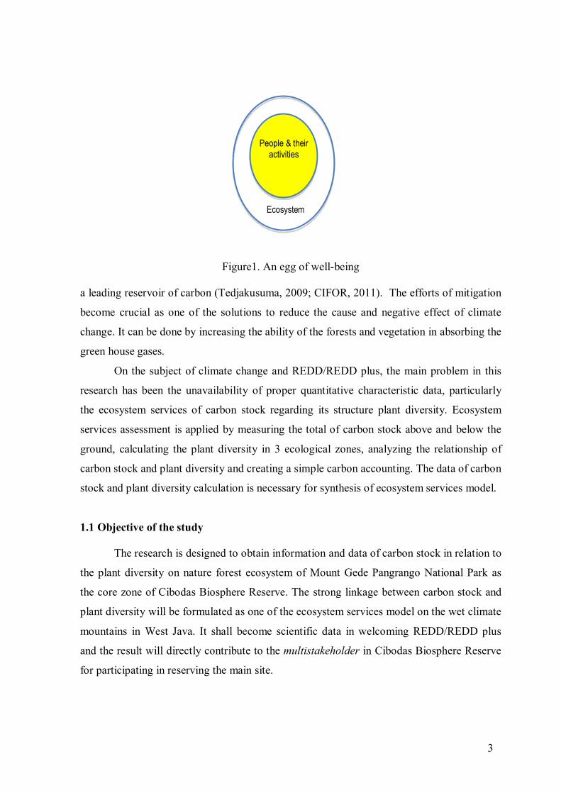
relationship between culture and biosphere that is portrayed as egg-well being (Figure 1)

(the Secretariat of CBD, 2002; IUCN, 2001 cited in Gibson, 2007). Therefore, the

integration between conservation and development includes the aspects of ecology,

economy and ethic, which complete one another.

Badan Perencanaan dan Pembangunan Nasional (National Development Planning

Agency of Republic of Indonesia) has placed the issue of climate change in the Mid-Long

Term Plan of 2010-2014. The funds will be extended until the year of 2030 as a strategic

vision in forestry, farm and other crucial sectors. The roadmap development of climate

change is based on Scientific Basis Assessment, which is followed by the monitoring and

evaluation efforts. Indonesia made a groundbreaking commitment to reduce emissions by

26% from business-as-usual levels by 2020 without sacrificing economic growth and to be

3

Ecosystem

Figure1. An egg of well-being

a leading reservoir of carbon (Tedjakusuma, 2009; CIFOR, 2011). The efforts of mitigation

become crucial as one of the solutions to reduce the cause and negative effect of climate

change. It can be done by increasing the ability of the forests and vegetation in absorbing the

green house gases.

On the subject of climate change and REDD/REDD plus, the main problem in this

research has been the unavailability of proper quantitative characteristic data, particularly

the ecosystem services of carbon stock regarding its structure plant diversity. Ecosystem

services assessment is applied by measuring the total of carbon stock above and below the

ground, calculating the plant diversity in 3 ecological zones, analyzing the relationship of

carbon stock and plant diversity and creating a simple carbon accounting. The data of carbon

stock and plant diversity calculation is necessary for synthesis of ecosystem services model.

1.1 Objective of the study

The research is designed to obtain information and data of carbon stock in relation to

the plant diversity on nature forest ecosystem of Mount Gede Pangrango National Park as

the core zone of Cibodas Biosphere Reserve. The strong linkage between carbon stock and

plant diversity will be formulated as one of the ecosystem services model on the wet climate

mountains in West Java. It shall become scientific data in welcoming REDD/REDD plus

and the result will directly contribute to the multistakeholder in Cibodas Biosphere Reserve

for participating in reserving the main site.

People & their activities

Ecosystem

4

2.0 METHODS 2.1 Study site

Mount Gede Pangrango National Park (MGPNP) is one of the tropical forest

ecosystems on the mountain with wet climate and has essential scientific value, particularly

on Java Island. MGPNP is geographically situated between 106º 51’ - 107º 02’ E and

6º 51’S. The park is dominated by two volcanoes: Mount Gede and Mount Pangrango.

Briefly, the main ecological zone of the park can be seen in Table 2 below.

Table 2. The main ecological zone of Mount Gede Pangrango National Park

Source: Wiratno et al., 2004

The climate condition according to Schmidt-Ferguson is a type A (Q = 5-9%) with the range

of temperature 18-25C, with the fall of rain is 3000-4000 mm per year on the average, and

air humidity is 80-90%, all of which cause the formation of peaty soil (MGPNP, 2008 and

2010). The native floras of MGPNP on the subalpine zone are Vaccinium varingiaefolium,

V. laurifolium, Paraserianthes lophanta, Anaphalis javanica, Leptospermum javanicum,

Rhododendron retusum, Carex verticillata, Hypericum leschenaultii, Rubus lineatus,

Gaultheria fragrantissima, G. leucocarpa and G. nummularioides. On the submontane until

montane zone, there are Altingia excelsa, Schima wallichii, Vernonia arborea, Neolitsia

cassiaefolia, Engelhardtia spicata, Flaucortia rukam, Acer laurinum, Magnolia candollei

and Orophea hexandra. The kind of palm likes Javana areca-palm, rope bamboo

Gigantochloa apus and forest banana Musa acuminata and Pandanus furcatus can be also

found in this forest. Different kinds of species on the elevation of 2000 m asl are

Lithocarpus pallidus, Castanopsis acuminatissima, Astronia spectabilis, Ardisia javanica,

Environment Vegetation Physical condition Subalpine zone Two layers: trees & forest floor

Leaves small Plant growth very slow

Cool and cloudy

Montane zone Medium size trees all about the same height

Medium size leaves Plant growth slow

Cool and cloudy

Submontane zone Five layers of vegetation including giant trees, called emergent

Species rich

Warm and humid Deep rich well

weathered soil

5

Leptospermum flavescens, Weinmania blumei and Achronodia punctata (Sunarko and

Rugayah, 1992).

The width of the park as stated on Surat Keputusan Menteri Kehutanan Nomor

174/Kpts-II/2003 are 22851.03 hectare with the adjustment on the field calculation, because

it has additional width from the area of Perum Perhutani which previously functioned as

permanent production forest and limited production forest for 7665 hectare. This area is

acknowledged by the UNESCO as core area from Cibodas Biosphere Reserve since 1977,

which is coherently with buffer and transition zone. It is aimed to promote the harmony

between human and biosphere with the appropriate and measured approach for sustainable

development of environment. In the administrative management of West Java province,

MGPNP are in 3 regencies, they are Cianjur, Bogor and Sukabumi (Soedjito, 2004;

MGPNP, 2008 and 2010).

This study is conducted on Mount Putri (Cianjur Regency) hiking track to

Selabintana (Sukabumi Regency) by creating a sampling plot based on the elevation from

1355 to 2802 m asl as a representative of Mount Gede. Meanwhile the plot as a

representative of Mount Pangrango is created on the elevation of 1079 and 1271 m asl at

Cisarua Resort, Bogor Regency (Figure 2).

Figure 2. Study site map on Mount Gede Pangrango National Park (Source: USGS, 2009; MGPNP, 2010).

6

2.2 Measurement of carbon stock and estimating the biomass

The research method consists of the following stages:

(1) Dividing Mount Gede Pangrango National Park in its each unique ecosystem as follows:

(a) submontane zone (1000-1500 m asl), (b) montane zone (1500-2400 m asl) and

(c) subalpine zone (2400-3019 m asl), where, m asl is meter above sea level.

(2) Measuring the carbon stock above and belowground by using World Agroforestry

Center (2007) as a guide.

100 m

20 m

Figure 3. Sampling plot for carbon measurement made with length direction in line with elevation line with the assumption representing vegetation gradation on each elevation.

Diameter measurement as high as human breast (DBH) using diameter tape for big trees

category is the ones that have 30 cm for diameter on the big and small plot. Meanwhile,

small trees with 5-30 cm for diameter are measured on the small plot (5 x 40 m2). The

biomass calculation is measured using allometric equations (Table 3).

Table 3. Allometric models used to convert measures of vegetation to AGB

Note: AGB = aboveground biomass (kg), TAGB = total aboveground biomass (kg), DW = dry weight (kg),

D = diameter (cm), DBH = diameter at breast height (cm), H = tree height (cm), c = intercept, α = slope coefficient of regression equation, ρ = wood mass (cm3).

Aboveground component Model Source

Tree > 5 cm DBH

Palms > 5 cm DBH Ferns > 5 cm DBH

DW = 0,118 D2,53 DW = 0,11 ρ D2,62 AGBest= ρ x exp(-1,499 + 2,148ln (D) + 0,207(ln(D))2 -0,0281(ln(D))3) Ln (TAGB) = c + αln(DBH) DW = 4.5 + 7.7H DW = ρ H D2/40

Brown et al. (1997) Ketterings et al. (2001) Chave et al. (2005) Basuki et al. (2009) Frangi and Lugo (1985) Hairiah et al. (1999)

40 m

5 m 0.5m

0.5m

7

Carbon concentration (C) in organic ingredients is usually 46%, thus carbon stock can be

calculated by multiplying the total of its mass weight with 0.46 (Hairiah and Rahayu, 2007).

The writing of allometric equation names in this report uses the main writer’s names

as representation and simplicity, they are Br = Brown et al., Kt = Ketterings et al.,

Cv = Chave et al. and Bs = Basuki et al. Wood density is based on the database in

http://www.worldagroforestrycenter.org and global wood density database in

http://hdl.handle.net/10255/dryad.235.

The measurement for understorey biomass is conducted destructively placing a

quadrant size 0.5 x 0.5 m2 on the 6 crossing points in a plot of 5 x 40 m2. This small

quadrant is also to take biomass of coarse litter, fine litter, fine root and sample of composite

soil. Fine litter is sieved on the 2 mm pore holes. Fresh weight per biomass part is weighed

and then 100-300 grams are taken for sub-sample, except fine litter for 100 grams, then it is

dried on the temperature of 80C for 2 x 24 hours. Calculating total dry weight of

understorey, coarse litter, fine litter and fine root per quadrant uses the following formula:

Total DW = (DW (gr)/FW subsample (gr)) x Total FW

Where, DW is dry weight, FW is fresh weight

The measurement of wood necromass is to standing or fallen dead trees, intact plant

stumps, branches and twigs with the diameter of 5 cm and 50 cm long. The method of

measurement is by measuring the diameter and length (height). Should there be a stem lie

across, then the stem diameter is measured on 3 positions (top, middle, down). The

calculation of wood density is conducted by taking the wood sample minimum at size 3x 3

x 3 cm3 for 3 times of repetitions, then weighing the fresh weight, after that putting into an

oven for a temperature of 80C for 2 x 24 hours.

Carbon stock below ground is taken from the composite soil sample on the quadrant

0.5 x 0.5 m2 with 6 points and 0-10 cm deep and 10-20 cm deep for pH analysis and C

organic percentage at Indonesian Soil Research Institute, Ministry of Agriculture, Republic

of Indonesia. The soil sample taking is not obstructed for soil texture in the laboratory;

meanwhile for soil bulk density measurement uses the ring sample carefully. The soil

sample is weighed for its fresh weight then dried in an oven with temperature of 105C for

2 x 24 hours and weighed for its dry weight (W2). The calculation of bulk density is with

the following formula:

BD = W2 (g)/V (soil volume in cm3)

8

The value of soil carbon can be predicted by using the following equation:

SC = %C-org x BD x AD

Where, SC is soil carbon (tons), BD is bulk density (tons/m3), D is soil sample depth (m), A is width of sample soil area (m2), %C org is % organic carbon

Total carbon per width unit is a totaling of trees biomass carbon, understorey biomass

carbon, necromass and soil carbon.

2.3 Plant diversity

The plant diversity calculation uses ecological index that includes the following

parameter (Mueller-Dombois and Ellenberg, 1974 cited in Partomihardjo and Rahajoe,

2004; Stiling, 1996; Pontasch et al., 1989; Michie, 1982).

(1) Basal area: r2 (m2 ha-1)

Relative Basal area (%): (Species basal area/total basal area) x 100%

Where, r is radius and diameter measurement of breast height

(2) Density: total number of individuals of species/sample plot width

Relative Density: (total number of individuals of species/total all individuals) x

100%

(3) Relative Frequency: (total plot of the found species/total all studied plots) x 100%

(4) Importance value: Relative Basal Area + Relative Density + Relative Frequency

Importance value per sample plot: Relative Basal Area + Relative Density

(5) Shannon-Wiener diversity index:

H’ = piln (pi)

Where, H’ is Shannon-Wiener diversity index, pi is the proportion of individuals belonging to species I and ln is natural log (i.e., base 2.718).

(5) Bray-Curtis Index:

1- BCij =

9

Where, 1-BCij is the similarity between two site/sample plot, i and j each defined by a set of n attributes, Xik, and Xjk is number of individuals in species. Species name uses Tropicos® website as the reference (http://www.tropicos.org/), IPNI (The

International Plant Names Index) (http://www.ipni.org) and Kewensis Index 2.0 from

Oxford University Press (1997). The checking about conservation status of plants

species found on the observation plot is based on the IUCN criteria IUCN

(http://www.iucnredlist.org).

2.4 Relationship between carbon stock and plant diversity

The relationship between carbon stock and plant diversity is calculated by using

regression and correlation equation with Excel 2008 installed in Mac OS X Version 10.5.8

system. The relationship modeling between Shannon Index to carbon stock uses polynomial

order 3 regression (cubic) by putting in prediction value and model test with value of LMCI

(lower mean confidence interval) and UMCI (upper mean confidence interval).

2.5 Carbon value

Estimation of carbon stock is calculated on its 3 ecological zones, they are subalpine

zone, montane zone and submontane zone. The carbon stock average obtained from 4

allometric equations is each multiplied by the zone width, therefore, the information about

the ability of supporting carbon from Mount GedePangrango National Park is achieved in

unit of millions of tons C.

2.6 Ecosystem service

The structuring of ecosystem services model based on carbon stock and plant

diversity is synthesized based on statistic calculation data, which is obtained and referred to

the theory and consideration of applied management for carbon stock case in climate change

context.

10

3.0 RESULTS AND DISCUSSION

3.1 Estimation carbon stock and biomass

The average result of carbon stock measurement (aboveground carbon stock) on 9

sites using four allometric equations in tons C per hectare is 399.717 (Brown/Br), 354.648

(Ketterings/Kt), 449.688 (Chave/Cv) and 325.724 (Basuki/Bs) (Figure 4).This average value

of the carbon stock is varied depending on the elevation between 233.837-597.554 (Br),

172.368-503.435 (Kt), 192.372-649.759 (Cv) and 156.82-454.645 (Bs).

Figure 4. Estimation of carbon stock and biomass on several elevations, AGB is aboveground biomass that consist of trees, understorey, litter and necromass.

The estimated biomass is assumed that its 46% is stored carbon stock on certain elevation.

The average value of the biomass is as much as 868.950 (Br), 770.974 (Kt), 977.583 (Cv)

and 708.095 (Bs), with variations between 508.341-1299.031 (Br), 374.714-1094.424 (Kt),

418.2-1412.52 (Cv) and 340.912-988.355 (Bs). The highest carbon stock is found on 2329 m

asl (montane zone), except Bs allometric on 2601 m asl (subalpine zone), and the lowest one

is found on 1355 m asl (Br) and 1079 m asl (Kt, Cv, Bs). The average of highest carbon

stock based on zone is on the subalpine zone, that is 409.751 (Kt), 553.858 (Cv),

411.661(Bs) except Br (463.466) on the montane zone. It is presumably caused by

contribution of Vaccinium varingiaefolium, which is multistem as well as dominant species

on the subalpine zone. One of the abundant species in a dense forest, precisely at fenced

area of Mount Gede crater, is Vaccinium varingiaefolium (Sunarno and Rugayah, 1992). The

contribution of carbon stock from Vaccinium varingiaefolium on the elevation of 2802 m asl

0

200

400

600

800

1000

1200

1400

1600

2802

2601

2329

2075

1851

1710

1355

1271

1079

Carb

on &

AG

B (

tons

C ha

-1)

Elevation (m asl)

Brown Biomassa Brown Carbon stockKetterings Biomassa Ketterings Carbon stockChave Biomassa Chave Carbon stockBasuki Biomassa Basuki Carbon stock

11

is the biggest one of all other species, that is 173.632 (Br), 165.136 (Kt), 237.518 (Cv) and

158.797 (Bs), meanwhile on 2601 is 206.293 (Br), 196.801 (Kt), 276.57 (Cv) and 187.467

(Bs). On the other side, when thoroughly observing the total of area per ecological zone,

then the biggest carbon stock is on the montane zone, because it is the widest zone (61%

total width) compared to two other zones (Table 4).

Note: Carbon stock is a mix aboveground and soil carbon in tons C ha-1.

According to Figure 5, it can be seen that the maximum proximity value from the big

trees to the small ones happens on the subalpine zone, that is 280 individuals ha-1 of the big

tree (2601 m asl) and 2950 individuals ha-1 (2802 m asl). On the other side, the minimum

proximity is shown on the submontane zone, which is 55 individuals ha-1 big trees

(1079 m asl) and 250 individuals ha-1 small trees (1271 m asl).

Figure 5. The value of trees proximity based on the elevation zone. The maximum value of big trees are on the elevation of 2601 m asl, meanwhile the small trees is found on the elevation of 2802 m asl.

Table 4. The average carbon stock in observation plot at 3 zones of MGPNP

Allometric

Zone

Subalpine Montane Submontane

Brown 430.701 463.466 294.082

Ketterings et al. 409.751 397.980 260.157

Chave et al. 553.858 506.695 304.252

Basuki et al. 411.661 362.261 219.735

0

500

1000

1500

2000

2500

3000

3500

Densi

ty (in

div

iduals

ha

-1)

Elevation (m asl)

Small tree Big tree

12

Brown Ketterings

Chave Basuki

Figure 6. Carbon stock is stored in two classes of tree sizes on different elevations. The maximum value of big trees are equal for all allometic equations, that is on the elevation of 1271 m asl, meanwhile small trees are on 2329 m asl. The minimum value of big trees is on the elevation of 1355 m asl, and for small trees are on the elevation of 1271 m asl.

0

100

200

300

400

500

600

2802

2601

2329

2075

1851

1710

1355

1271

1079

carb

on s

tock (

tons C

ha

-1)

Elevation (m asl)

Big tree Small tree

0

50

100

150

200

250

300

350

400

450

500

2802

2601

2329

2075

1851

1710

1355

1271

1079

Carb

on s

tock (

tons C

ha

-1)

Elevation (m asl)

Big tree Small tree

0

100

200

300

400

500

600

700

2802

2601

2329

2075

1851

1710

1355

1271

1079

Carb

on s

tock

(tons

C h

a-1

)

Elevation (m asl)

Big tree Small tree

0

50

100

150

200

250

300

350

400

450

2802

2601

2329

2075

1851

1710

1355

1271

1079

Carb

on s

tock

(tons

C h

a-1

)

Elevation (m asl)

Big tree Small tree

13

The measurement of carbon stock in trees biomass is conducted in two classes of tree

size; those are big trees (DBH >30 cm) and small trees (DBH 5-30 cm). The approximate

values of carbon stock (tons C ha-1) on big trees are 65.968-338.997 (Br), 56.853-346.307

(Kt), 81.351-390.052 (Cv) and 51.512-218.377 (Bs); and on the small trees are 17.208-

314.374 (Br), 13.93-258.749 (Kt), 19.621-341.978 (Cv) and 16.837-227.082 (Bs).

Meanwhile the approximate average of contribution on the aboveground carbon stock from

the big trees 42.697-51.963% and from the small trees 29.664-35.892%. The contrast

combination happens on the elevation of 1271 m asl, which the maximum values of carbon

stock from the big trees are along with small trees (Figure 6). It is a result of the maximum

proximity of big trees per hectare and the minimum proximity of small trees.

The tree component has the significant average contribution value to the total carbon

stock, that is 82.803% (Br), 80.692% (Kt), 84.994% (Cv) and 79.766% (Bs) (Figure 7). It

shows the role of tree biomass is highly essential in supporting carbon. On the other side, the

average contribution on the aboveground carbon stock from under storey is as much as

1.302% (Br), 1.517% (Kt), 1.198% (Cv) and 1.559% (Bs); from litter is 12.895% (Br),

14.83% (Kt), 11.778% (Cv) and 15.735% (Bs); and from necromass is 3.308% (Br), 3.932%

(Kt), 3.156% (Cv) and 4.117% (Bs). Contribution from litter is relatively higher than

necromass and understorey and based on Clark's research (2001), it shows that fine litterfall

has high correlation (R2 = 0.69) towards the aboveground biomass increment in tropical

forest. Use of allometric equation in calculation influences the difference of tree contribution

percentage to the total aboveground biomass and carbon stock (Table 5).

Table 5. The average contribution of carbon stock from trees on 4 allometric equations

Elevation (m asl)

Allometric equations (%)

Brown Ketterings Chave Basuki

2802 78.905 77.249 83.017 78.226 2601 87.308 86.922 90.390 86.577 2329 88.263 86.069 89.206 84.035 2075 85.191 81.809 85.514 79.892 1851 73.952 70.830 77.567 71.106 1710 86.622 84.997 88.018 83.302 1355 74.514 69.865 77.132 72.545 1271 87.673 87.794 89.107 82.445 1079 80.030 71.951 74.868 69.170 Average 82.803 80.692 84.994 79.766

14

Brown Ketterings

Chave Basuki

Figure 7. Contribution of tree component, understorey, litter and necromass for carbon stock on different elevations.

0

100

200

300

400

500

600

2802

2601

2329

2075

1851

1710

1355

1271

1079

Carb

on s

tock

(tons C

ha

-1)

Elevation (m asl)

Tree

Understorey

Litter

Necromass

0

50

100

150

200

250

300

350

400

450

500

2802

2601

2329

2075

1851

1710

1355

1271

1079

Carb

on s

tock (

tons C

ha

-1)

Elevation (m asl)

Tree

Understorey

Litter

Necromass

0

100

200

300

400

500

600

700

2802

2601

2329

2075

1851

1710

1355

1271

1079

Carb

on s

tock

(tons

C h

a-1

)

Elevation (m asl)

Tree

Understorey

Litter

Necromass

0

50

100

150

200

250

300

350

400

450

2802

2601

2329

2075

1851

1710

1355

1271

1079

Carb

on s

tock

(to

ns

C h

a-1

)

Elevation (m asl)

Tree

Understorey

Litter

Necromass

15

3.2 Plant diversity as the carbon stock performance and its conservation value

This research shows that approximately 66 native species of Mount Gede Pangrango

National Park, most of which are in the family of Lauraceae, Fagaceae, Myrtaceae and

Moraceae. Some of the species becomes dominance on certain elevations, such as

Leptospermum flavescens, Lithocarpus sundaicus, Neolitsea javanica, Castanopsis javanica,

Castanopsis tungurrut, Castanopsis acuminatissima and Phoebe grandis. On the elevation

of 2601 m asl and 1710 m asl, there is Paraserianthes lophantha (kemlandingan gunung)

which is called mountain mass elevation by Steenis (1972), that is the elevation

approximation found between 1100-3100 m asl. Meanwhile, the height of lowest peak where

species are found is on the 2500 m asl, and the effect is on the elevation of 1400 m asl. The

most number of species are found at Selabintana V (1710 m asl), there are 25 species,

followed by Pasir Ipis (1355 m asl) with 23 species, thus both of them have relatively higher

Shannon Index than other elevations, and those are 2.925 and 2.701. The least number of

species from observation plot is on the elevation of 2802 m asl with 7 species.

The interesting fact is that Schima wallichii is found from the elevation of 1271

(submontane) until 2601 m asl (subalpine) and it is shown with a high frequency of 0.778

and importance value of 36.865 (Table 6). This finding eventually makes Schima wallichii

has the highest carbon stock value (451.682/Bs-652.434/Br), particularly if it is compared

with the minimum value of carbon stock from Ziziphus angustifolia (0.232/Br) and Laportea

stimulans (0.103/Kt-0.242/Bs) (Figure 22 and Appendix 1). In the meantime, the special

species at the crater, Vaccinium varingiaefolium, has the highest importance value of 49.152,

and though with only small frequency of 0.222, with basal area is 314.714 m2 ha-1 widths.

On the other side, it is important to know that the plot on this crater (2802 m asl) has the

lowest Shannon Index that is 1.409. Based on the Table 6 and Figure 8, the population of

Vaccinium varingiaefolium is so many that they have the high value of basal area, followed

by Schima wallichii, Myrsine hasseltii and Symplocos odoratissima. Other species that has

relatively high frequency (0.556) are Lithocarpus sundaicus (subalpine-submontane) and

Cyathea latebrosa (montane-submontane). Even though Castanopsis acuminatissima has

only low frequency (0.111), it has a high basal area and high importance value. It is a result

of the relatively big accumulation value (11.86 m) of tree diameter. Some species has

relatively small frequency value (0.111-0.333), however, they are with high importance

value on some elevations such as Phoebe grandis, Oriocnide scabra and Platea latifolia.

16

Table 6. Ecological index of 30 species with highest importance value on study site

Species Basal area (m2 ha-1)

Density (individuals ha-1)

Frequency Importance Value

Vaccinium varingiaefolium 314.714 405 0.222 49.152

Schima wallichii 174.821 390 0.778 36.865

Myrsine hasseltii 38.072 285 0.444 16.032

Leptospermum flavescens 91.457 135 0.222 15.903

Lithocarpus sundaicus 52.790 125 0.556 13.573

Catanopsis acuminatissima 110.423 20 0.111 13.295

Symplocos odoratissima 18.452 245 0.333 11.845

Platea latifolia 19.634 115 0.333 8.014

Neolitsea javanica 11.770 105 0.444 7.597

Castanopsis tungurrut 7.529 135 0.222 6.498

Castanopsis javanica 7.820 105 0.333 6.385

Cyathea latebrosa 0.096 55 0.556 5.534

Neolitsea cassiaefolia 1.499 60 0.444 5.074

Elaeocarpus angustifolius 3.321 75 0.333 4.966

Polyosma integrifolia 1.193 55 0.444 4.887

Syzygium rostratum 2.443 60 0.333 4.411

Elaeocarpus stipularis 2.233 60 0.333 4.387

Macropanax dispermum 0.744 60 0.333 4.220

Ardisia javanica 0.272 35 0.444 4.175

Oreocnide scabra 2.999 75 0.222 4.161

Vernonia arborea 7.744 55 0.222 4.083

Euonymus javanicus 0.176 55 0.333 4.004

Macropanax concinnus 0.321 45 0.333 3.716

Lithocarpus pallidus 0.858 20 0.333 3.014

Phoebe grandis 4.416 55 0.111 2.941

Acronychia pedunculata 1.466 15 0.333 2.929

Dysoxylum alliaceum 1.290 35 0.222 2.750

Trema orientalis 3.717 25 0.222 2.717

Astronia spectabilis 1.264 30 0.222 2.595

Flacourtia rukam 0.005 45 0.111 2.142

17

Figure 8. Composition and abundance of plant species on 3 ecology zones MGPNP.

0 20 40 60 80 100

Acer laurinum

Acronychia pedunculata

Acronychia trifoliolata

Aglaia eclliptica

Alangium chinense

Antidesma tetrandum

Ardisia javanica

Astronia spectabilis

Castanopsis javanica

Castanopsis tungurrut

Catanopsis …

Cryptocarya ferrea

Cyathea junghuhniana

Cyathea latebrosa

Cyathea spinulosa

Dacrycarpus imbricatus

Dysoxylum alliaceum

Elaeocarpus …

Elaeocarpus stipularis

Engelhardtia spicata

Euonymus javanicus

Ficus cuspidata

Ficus fistulosa

Ficus heterophylla

Ficus padana

Ficus ribes

Flacourtia rukam

Gordonia excelsa

Itea macrophylla

Lagerstroemia indica

Lagerstroemia speciosa

Laportea stimulans

Leptospermum …

Leptospermum …

Lindera polyantha

Lithocarpus pallida

Lithocarpus sundaica

Litsea mappacea

Macropanax cocinnum

Macropanax dispermum

Magnolia lilifera

Myrsine hasseltii

Neolitsea cassiaefolia

Neolitsea javanica

Oreocnide scabra

Paraserianthes lophanta

Phoebe grandis

Pinanga coronata

Platea latifolia

Polyosma integrifolia

Prunus arborea

Rapanea hasseltii

Schefflera scandens

Schima wallichii

Symplocos odoratissima

Syzygium antisepticum

Syzygium racemosum

Syzygium rostratum

Toona sureni

Trema orientalis

Turpinia sphaerocarpa

Urophyllum arboreum

Vaccinium …

Vernonia arborea

Weinmannia blumei

Ziziphus angustifolia

Number of individuals

18

Based on tree proximity class per hectare, it shows that its 68.182% is classified into class

occasionally (0-50), and its 25.76% is classified into class often (51-150) and the rest is class

abundant (100-450) that has relatively small proportion, that is 6.06%.

Table 7. Class and category of tree density

Class of density (individuals ha-1)

Proportion (%)

Category

0-50 68.182 occasionally 51-100 16.667 often

101-150 9.091 often

151-200 0.000 abundant

201-250 1.515 abundant 251-300 1.515 abundant 301-350 0.000 abundant 351-400 1.515 abundant 401-450 1.515 abundant

Figure 9. The relationship between species density rank and its abundance. Species with high abundance are Vaccinium varingiaefolium, Schima wallichii, Myrsine hasseltii, Leptospermum flavescens, Lithocarpus sundaicus, Catanopsis acuminatissima, Symplocos odoratissima, Platea latifolia, Neolitsea javanica and Castanopsis tungurrut. Data can be referred to Appendix 4.

0

3060

90120

150

180210

240270

300

330360

390420

450

0 5 10 15 20 25 30 35 40 45 50 55 60 65 70

Abundance (

indiv

iduals

ha

-1)

Species density rank

19

On subalpine zone, there are dominant species on wet-climate mountains such as Vaccinium

varingiaefolium, Symplocos odoratissima, Myrsine hasseltii and Leptospermum flavescens

and each has the importance value of 211.155, 51.594, 66.085 and 60.275 (Table 8 and

Figure 10).

Figure 10. Composition and abundance of plant species on subalpine zone.

Montane zone is the widest zone of the other two zones, and species with highest

abundance is found in the zone, those are Schima wallichii (81.115), Lithocarpus sundaicus

(291.32), Platea latifolia (49.593), Neolitsea javanica (33.273), and Elaeocarpus

angustifolius (24.957) (Table 8 and Figure 11). Some species found on the montane and

subalpine zone are included into IUCN red list, therefore it is important to protect them from

any disturbance and the threatened species populations will be sustained for a long term by

protecting the types of habitat (Widyatmoko, 2010). Some species can found here,

Euonymus javanicus (Celastraceae), Dysoxylum alliaceum (Meliaceae), Engelhardtia

spicata (Juglandaceae), the ones with the status of Lower Risk (LR)/least concern, that is

does not qualify for a more at risk category, widespread and abundant taxa, are included in

this category. Furthermore, Macropanax concinnus (Araliaceae) is in category Vulnerable

B1+2c, it means it is facing a high risk of extinction in the wild in the medium-term future,

severely fragmented or known to exist at no more than ten locations, also continuing decline,

inferred, observed or projected because of area, extent and/or quality of habitats. The

frequency of Euonymus javanicus is 0.333 (elevation 1851, 1710, 1355) with density of 55

0 10 20 30 40 50 60 70 80 90

Ardisia javanica

Cyathea latebrosa

Leptospermum flavescens

Leptospermum javanicum

Macropanax concinnus

Myrsine hasseltii



Schima wallichii

Schefflera scandens


Vaccinium varingiaefolium


20

trees per hectare, meanwhile, the frequency of Dysoxylum alliaceum is 0.222 (elevation

1851, 1710) with density of 35, the frequency of Engelhardtia spicata is 0.111 (elevation

2329) with relatively low density of 5 trees per hectare. Macropanax concinnus that has

frequency of 0.333 (elevation 2802, 1851, 1710) and density of 45 trees per hectare requires

main attention for conservation.

Figure 11. Composition and abundance of plant species on montane zone MGPNP.

0 10 20 30 40 50 60 70

Acer laurinum


Antidesma tetrandum

Ardisia javanica

Astronia spectabilis



Cryptocarya ferrea

Cyathea junghuhniana

Cyathea latebrosa

Dacrycarpus imbricatus

Dysoxylum alliaceum

Elaeocarpus angustifolius


Engelhardtia spicata

Euonymus javanicus

Ficus cuspidata

Flacourtia rukam

Lagerstroemia speciosa

Lindera polyantha

Lithocarpus pallidus

Lithocarpus sundaicus

Litsea mappacea

Macropanax concinnus


Magnolia lilifera

Myrsine hasseltii


Neolitsea javanica

Oreocnide scabra


Platea latifolia


Schima wallichii

Syzygium antisepticum

Syzygium racemosum

Syzygium rostratum

Turpinia sphaerocarpa

Urophyllum arboreum

Vernonia arborea

Weinmannia blumei


21

The most abundance on submontane zone with each highest importance value are Schima

wallichii (83.585), Castanopsis tungurrut (57.179), Oriocnide scabra (78.753), Castanopsis

javanica (35.036) and Phoebe grandis (42.515) (Table 8 and Figure 12). Prunus arborea

(Rosaceae), which includes the category of LR/lower risk, with frequency of 0.111 and

estimated density of 5 trees per hectare, is only found on the elevation of 1355 m asl.

Figure 12. Composition and abundance of plant species on submontane zone of MGPNP.

The stratification of Java Mountains forests based on its configuration trees can be

observed on site (Steenis, 1972). Based on the importance value on Table 8, the first tree

layer/canopy is Schima wallichii, Vernonia arborea, Engelhardtia spicata, Elaeocarpus

0 5 10 15 20 25

Acronychia trifoliolata


Aglaia eclliptica

Alangium chinense

Antidesma tetrandum



Catanopsis acuminatissima

Cyathea latebrosa

Cyathea spinulosa

Dysoxylum alliaceum

Elaeocarpus angustifolius


Euonymus javanicus

Ficus fistulosa

Ficus heterophylla

Ficus padana

Ficus ribes

Gordonia excelsa

Itea macrophylla

Lagerstroemia indica

Laportea stimulans

Lindera polyantha

Lithocarpus pallida

Lithocarpus sundaica



Neolitsea javanica

Oreocnide scabra

Phoebe grandis

Pinanga coronata

Prunus arborea

Rapanea hasseltii

Schima wallichii


Toona sureni

Trema orientalis

Urophyllum arboreum

Vernonia arborea

Ziziphus angustifolia


22

angustofolius and Elaeocarpus stipularis, the second layer is Symplocos odoratissima,

Acronychia pedunculata, while Ardisia javanica is small tree at the third layer.

Table 8. Relative value of ecological index component on Mount Gede Pangrango National Park

Elevation Species Relative Relative Importance (m asl)/Zone Basal area Density Value

2802 Myrsine haseltii 9.696 26.606 36.301 Subalpine Symplocos odoratissima 6.191 26.606 32.797

Vaccinium varingiifolium 83.600 37.615 121.215

Other species (4) 0.513 9.174 9.687

2601 Leptospermum flavescens 35.997 20.175 56.172

Subalpine Myrsine hasseltii 6.976 22.807 29.784

Vaccinium varingiifolium 54.853 35.088 89.940

Symplocos odoratissima 2.131 16.667 18.798

Ardisia javanica 0.001 0.877 0.878

Schima wallichii 0.021 1.754 1.776

Other species (3) 0.021 2.632 2.652

2329 Lithocarpus sundaicus 37.641 21.429 59.069

Montana Schima wallichii 53.203 28.571 81.774

Vernonia arborea 6.988 14.286 21.274


Engelhardtia spicata 0.008 1.429 1.436

Other species (7) 2.158 32.857 35.015

2075 Neolitsea javanica 14.963 18.310 33.273

Montana Platea latifolia 27.058 22.535 49.593


Elaeocarpus stipularis 0.301 1.408 1.709

Others species (12) 10.042 40.845 50.587

1851 Castanopsis javanica 10.593 10.000 20.593

Montana Castanopsis tungurut 22.369 10.000 32.369



Elaeocarpus angustifolius 8.892 10 18.892


Others species (11) 16.554 40 56.554

1710 Schima wallichii 77.504 14.141 91.645

Montana Lithocarpus sundaicus 14.975 7.071 22.046

Acronychia pedunculata 0.135 1.01 1.145


Elaeocarpus angustifolius 0.005 6.061 6.065

Others species (20) 7.521 78.788 86.309

1355 Castanopsis javanica 19.543 15.493 35.036

Submontane Phoebe grandis 27.022 15.493 42.515


Acronychia pedunculata 1.045 7.042 8.087


Other species (19) 10.888 42.254 53.142

1271 Castanopsis tungurut 0.036 57.143 57.179

Submontane Catanopsis acuminatissima 92.349 2.857 95.206


Acronychia trifoliolata 0.063 2.857 2.921

Elaeocarpus angustifolius 0.286 5.714 6

Other species (4) 0.198 11.429 11.626

1079 Oriochnide scabra 32.087 46.667 78.753

Submontane Toona sureni 19.805 3.333 23.138

Trema orientalis 38.680 13.333 52.014

Vernonia arborea 1.786 3.333 5.119

Other species (8) 7.642 33.333 40.975

23

The following description shows equal regressions and correlation values out of the

efforts to identify the relationship between carbon stock and plant diversity and they can be

observed on each elevation.

(A) Gunung Gemuruh

Fig. 13. The relationship of basal area, density and importance value to carbon stock on the elevation of 2802 m asl (plot Gunung Gemuruh). Basal area and importance value parameter show a high correlation value, which means both parameters influence carbon stock for 93.8-98% and 99-99.7%. Density influences the carbon stock for 68.3-78.9%. The increase of carbon stock as the result of adding one value on each parameter is 0.167-0.255 units from basal area, 0.563-841 units from density and 1.228-1.923 unit from importance value.

Allometric Equations Determinant coefficients

Brown y = 0.181x + 15.93 R² = 0.962 Ketterings y= 0.174x + 13.09 R² = 0.980 Chave y = 0.255x + 14.86 R² = 0.976

Basuki y= 0.167x + 14.49 R² = 0.938


Brown y = 0.613x - 4.408 R² = 0.732 Ketterings y = 0.563x - 4.474 R² = 0.683 Chave y = 0.841x - 12.01 R² = 0.704

Basuki y = 0.594x - 6.526 R² = 0.789


Brown y = 1.375x + 4.022 R² = 0.992

Ketterings y = 1.288x + 2.936 R² = 0.997 Chave y = 1.923x - 1.481 R² = 0.990 Basuki y = 1.288x + 2.936 R² = 0.997

0

50

100

150

200

250

300

0 100 200 300 400 500 600 700 800 900 1000

Carb

on s

tock (

tons C

ha

-1)

Basal area (m2 ha-1)

Brown Ketterings

Chave Basuki

Linear (Brown) Linear (Ketterings)

Linear (Chave) Linear (Basuki)

0

50

100

150

200

250

0 20 40 60 80 100 120 140 160 180 200 220C

arb

on s

tock

(tons C

ha

-1)


Brown Ketterings

Chave Basuki

Linear (Brown) Linear (Ketterings )

Linear (Chave ) Linear (Basuki )

0

50

100

150

200

250

0 25 50 75 100 125 150

Carb

on s

tock

(to

ns C

ha

-1)

Importance value

Brown Ketterings

Chave Basuki



24

(B) Selabintana I

Fig. 14. The relationship of basal area, density and importance value to carbon stock on the elevation of 2601 m asl (plot Selabintana I). Basal area and importance value parameter show a high correlation value, which means both parameters influence carbon stock 95.9-99% and 98.2-99.4%. Density influences the carbon stock for 77.9-85.1%. The increase of carbon stock as the result of adding one value on each parameter is 0.249-0.389 units from basal area, 0.808-1.2 units from density and 2.026-3.109 units from importance value.



Basuki y = 0.808x - 7.782 R² = 0.851


Brown y = 0.276x + 7.613 R² = 0.973

Ketterings y = 0.278x + 5.858 R² = 0.990 Chave y = 0.389x + 8.890 R² = 0.988 Basuki y = 0.249x + 8.633 R² = 0.959


Brown y = 2.226x - 3.212 R² = 0.988

Ketterings y = 2.216x - 4.472 R² = 0.982 Chave y = 3.109x - 5.740 R² = 0.985 Basuki y = 2.026x - 1.593 R² = 0.994

0

50

100

150

200

250

300

0 20 40 60 80 100 120 140 160 180 200 220

Carb

on s

tock (

tons C

ha

-1)


Brown KetteringsChave BasukiLinear (Brown) Linear (Ketterings)Linear (Chave) Linear (Basuki)

0

50

100

150

200

250

300

0 100 200 300 400 500 600 700 800

Carb

on s

tock (

tons C

ha

-1)



0

50

100

150

200

250

300

0 10 20 30 40 50 60 70 80 90 100

Carb

on s

tock (

tons C

ha

-1)

Importance value


25

(C) Selabintana II

Fig. 15. The relationship of basal area, density and importance value to carbon stock on the elevation of 2329 m asl (plot Selabintana II). Basal area and importance value parameter show a high correlation value, which means both parameters influence carbon stock 96.1-98.4%. Density influences the carbon stock for 77-80.8%. The increase of carbon stock as the result of adding one value on each parameter is 0.552-0.971 units from basal area, 1.525-2.645 units from density and 2.003-3.508 units from importance value.

.


Brown y = 0.841x + 4.178 R² = 0.984 Ketterings y = 0.727x + 2.365 R² = 0.961

Chave y = 0.971x + 3.093 R² = 0.972 Basuki y = 0.552x + 4.726 R² = 0.973


Brown y = 2.306x - 25.08 R² = 0.805 Ketterings y = 1.971x - 22.29 R² = 0.770

Chave y = 2.645x - 30.17 R² = 0.785 Basuki y = 1.525x - 14.80 R² = 0.808


Brown y = 3.045x - 8.551 R² = 0.960 Ketterings y = 2.622x - 8.485 R² = 0.932

Chave y = 3.508x - 11.48 R² = 0.945 Basuki y = 2.003x - 3.707 R² = 0.954

0

50

100

150

200

250

300

350

0 50 100 150 200 250 300 350

Carb

on s

tock (

tons C

ha

-1)



0

50

100

150

200

250

300

350

0 25 50 75 100 125

Carb

on s

tock (

tons C

ha

-1)



0

50

100

150

200

250

300

350

0 15 30 45 60 75 90

Carb

on s

tock (

tons h

a-1

)

Importance value


26

(D) Selabintana III

Fig. 16. The relationship of basal area, density and importance value to carbon stock on the elevation of 2075 m asl (plot Selabintana III). Basal area and importance value parameter show a relatively similar correlation value, which means each parameter influences carbon stock for 67.7-78.6% and 60.7-77.1%. Density influences the carbon stock for 34.8-57%. The increase of carbon stock as the result of adding one value on each parameter is 0.364-58.6 units from basal area, 0.542-0.814 units from density and 0.844-1.31 units from importance value.


Brown y = 0.540x + 11.09 R² = 0.677



Brown y = 0.812x + 4.530 R² = 0.457





0

20

40

60

80

100

120

0 20 40 60 80 100 120 140 160 180

Carb

on s

tock (

tons C

ha

-1)



0

20

40

60

80

100

120

0 10 20 30 40 50 60 70 80 90

Carb

on s

tock (

tons C

ha

-1)



0

20

40

60

80

100

120

0 5 10 15 20 25 30 35 40 45 50 55 60 65 70

Carb

on s

tock (

tons C

ha

-1)

Importance value


27

(E) Selabintana IV

Fig. 17. The relationship of basal area, density and importance value to carbon stock on the elevation of 1851 m asl (plot Selabintana IV). Basal area, density and importance value parameter show a relatively similar correlation value, which means each parameter influences carbon stock for 72.8-89.2%, 82.5-94.8%, 67.7-78.6% and 84.3-88%. Density influences the carbon stock for 34.8-57%. The increase of carbon stock as the result of adding one value on each parameter is 0.649-1.055 units from basal area, 0.763-1.063 units from density and 0.806-1.277 units from importance value.


Brown y = 0.848x + 4.674 R² = 0.892



Brown y = 0.839x - 4.271 R² = 0.880



Brown y = 1.021x + 1.007 R² = 0.948


0

10

20

30

40

50

60

70

80

0 10 20 30 40 50 60 70

Carb

on s

tock (

tons C

ha

-1)



0

10

20

30

40

50

60

70

0 10 20 30 40 50 60 70

Carb

on s

tock (

tons C

ha

-1)



0

10

20

30

40

50

60

70

80

0 10 20 30 40 50 60

Carb

on s

tock (

tons C

ha

-1)

Importance value


28

(F) Selabintana V

Fig. 18. The relationship of basal area, density and importance value to carbon stock on the elevation of 1710 m asl (plot Selabintana V). Basal area and importance value parameter show a relatively similar correlation value, which means each parameter influences carbon stock for 61.5-74.1% and 62.5-74.5%. Density influences the carbon stock for 36.4-40.8%. The increase of carbon stock as the result of adding one value on each parameter is 0.352-0.637 units from basal area, 0.948-1.625 units from density and 1.125-2.028 units from importance value.


Brown y = 0.551x + 10.73 R² = 0.734

Ketterings y = 0.493x + 9.231 R² = 0.727 Chave y = 0.637x + 12 R² = 0.741 Basuki y = 0.352x + 9.335 R² = 0.615


Brown y = 1.440x - 9.722 R² = 0.408





0

40

80

120

160

200

240

0 50 100 150 200 250 300

Carb

on s

tock (

tons C

ha

-1)



0

20

40

60

80

100

120

140

160

180

200

0 20 40 60 80

Carb

on s

tock (

tons C

ha

-1)



0

50

100

150

200

250

0 20 40 60 80 100

Carb

on s

tock

(tons C

ha

-1)

Importance value


29

(G) Pasir Ipis

Fig. 19. The relationship of basal area, density and importance value to carbon stock on the elevation of 1355 m asl (plot Pasir Ipis). Basal area and importance value parameter show a relatively similar correlation value, which means each parameter influences carbon stock for 73-74.6% and 73.6-76.2%. Density influences the carbon stock for 64.1-71.6%. The increase of carbon stock as the result of adding one value on each parameter is 0.987-1.432 units from basal area, 0.49-0.71 units from density and 0.611-0.886 units from importance value.



Basuki y = 0.533x - 0.486 R² = 0.716





Brown y = 0.738x + 2.250 R² = 0.762 Ketterings y = 0.611x + 1.616 R² = 0.739 Chave y = 0.886x + 2.385 R² = 0.736

Basuki y = 0.638x + 2.201 R² = 0.755

0

10

20

30

40

50

60

70

0 5 10 15 20 25 30 35 40

Carb

on s

tock (

tons C

ha

-1)



0

10

20

30

40

50

60

70

0 10 20 30 40 50 60

Carb

on s

tock

(tons C

ha

-1)



0

10

20

30

40

50

60

70

0 10 20 30 40 50 60

Carb

on s

tock

(tons C

ha

-1)

Importance value

Brown Ketterings

Chave BasukiLinear (Brown) Linear (Ketterings)


30

(H) Ciremes

Fig. 20. The relationship between basal area, density and importance value to carbon stock on the elevation of 1271 m asl (plot Ciremes). Basal area parameter shows relatively small correlation value and density shows relatively high correlation value, which means density influences carbon stock for 95.7-96.8%. Importance value in a form of quadratic relationship to carbon stock that is able to explain 68.4-71.7% of the observed variability and increases until the top of importance value 60 then decreases. The increase of carbon stock as the result of adding one value on the density is 1.855-3.370 units.


Brown y = -0.065x + 43.93 R² = 0.016

Ketterings y = -0.068x + 44.56 R² = 0.015 Chave y = -0.071x + 50.23 R² = 0.014 Basuki y = -0.035x + 28.51 R² = 0.012


Brown y = 2.913x - 17.06 R² = 0.965


Allometric

Equations Determinant coefficients

Brown y= -0.089x2 + 9.230x - 34.51 R² = 0.703 Ketterings y = -0.093x2 + 9.639x - 37.66 R² = 0.684 Chave y = -0.103x2 + 10.69x - 40.70 R² =0.709 Basuki y = -0.057x2 + 5.899x - 21.66 R² = 0.717

0

50

100

150

200

250

300

350

0 100 200 300 400 500 600

Carb

on s

tock

(tons C

ha

-1)


Brown Ketterings

Chave Basuki



0

50

100

150

200

250

300

350

0 25 50 75 100 125

Carb

on s

tock (

tons C

ha

-1)



0

50

100

150

200

250

300

350

0 20 40 60 80 100

Carb

on s

tock (

tons C

ha

-1)

Importance value

Brown Ketterings

Chave Basuki

Poly. (Brown) Poly. (Ketterings)

Poly. (Chave) Poly. (Basuki)

31

(I) Ciberet

Fig. 21. The relationship between basal area, density and importance value to carbon stock on the elevation of 1079 m asl (plot Ciremes). Basal area parameter shows quadratic relationship that explains 55.3-73.8% of the observed variability, and increases until the top of basal area 10 m2ha-1 then decreases. Density shows relatively small correlation value. Importance value in a form of cubic relationship to the carbon stock is able to explain 42.3-57.5% of the observed variability.


Brown y = -21.61x2 + 79.38x - 1.085 R² = 0.738

Ketterings y = -12.21x2 + 44.69x + 0.820 R² = 0.655

Chave y = -12.13x2 + 45.55x + 1.411 R² = 0.712

Basuki y = -6.989x2 + 26.99x + 2.288 R² = 0.553


Brown y = 0.018x2 - 1.190x + 20.96 R² = 0.036

Ketterings y = 0.013x2 - 0.919x + 14.51 R² = 0.058

Chave y = 0.014x2 - 0.877x + 14.91 R² = 0.118

Basuki y = 0.013x2 - 0.731x + 11.19 R² = 0.271

Allometric

Equations Determinant coefficients

Brown y = 0.001x3 - 0.234x2 + 8.470x - 28.88 R² = 0.575

Ketterings y = 0.001x3 - 0.129x2 + 4.598x - 13.97 R² = 0.469

Chave y = 0.001x3 - 0.126x2 + 4.481x - 12.73 R² = 0.497

Basuki y = 0.000x3 - 0.069x2 + 2.336x - 4.542 R² = 0.423

0

10

20

30

40

50

60

70

80

90

100

0 4 8 12 16 20

Carb

on s

tock (

tons C

ha

-1)


Brown KetteringsChave BasukiPoly. (Brown) Poly. (Ketterings)Poly. (Chave) Poly. (Basuki)

0

10

20

30

40

50

60

70

80

90

100

0 20 40 60 80

Carb

on s

tock (

tons C

ha

-1)


Brown Ketterings

Chave Basuki

Poly. (Brown) Poly. (Ketterings)

Poly. (Chave) Poly. (Basuki)

0

10

20

30

40

50

60

70

80

90

100

0 20 40 60 80 100

Carb

on s

tock (

tons C

ha

-1)

Importance value

Brown KetteringsChave BasukiPoly. (Brown) Poly. (Ketterings)Poly. (Chave) Poly. (Basuki)

32

3.3 Relationship between carbon stock and plant diversity

The relationship between carbon stock and plant diversity becomes an interesting

thought to be observed, because it is strongly assumed there is a co-benefit between the two.

This assumption occurs with the reason that both of them are resource component that

provide ecosystem services. Previous studies show that at a global scale, tropical forests

provide some of the highest levels of biomass carbon storage, productivity and biodiversity,

spatial patterns of carbon dynamics and biodiversity are complex with limited correlations

between these variables. However, plant communities in tropical forests are the fundamental

units of vegetation management (UN-REDD, 2010; McPherson and DeStefano, 2003). This

study will elaborate how carbon stock is related with ecological index and species formation

in each ecological zone at MGPNP (Table 9, 10, 11).

Table 9. Carbon stock, ecology indexes and formation at the subalpine zone

Elevation (m asl)

C stock (ton C ha-1)

R2 to C stock Species composition

Dominant species and Shannon Index

BA Density Importance value

2802 Gunung Gemuruh

380.549Br 352.844Kt 472.677Cv 368.672Bs

0.962 0.980 0.976 0.938

0.732 0.683 0.704 0.789

0.992 0.997 0.990 0.997

Cyathea latebrosa, Leptospermum flavescens, Leptospermum javanicum, Macropanax concinnus, Myrsine haseltii, Symplocos odoratissima, Vaccinium varingiaefolium

Vaccinium varingiaefolium, Myrsine haseltii, Symplocos odoratissima H’: 1.409

2601 Selabintana I

480.854Br 466.659Kt 635.038Cv 454.651Bs

0.973 0.990 0.988 0.959

0.816 0.779 0.788 0.851

0.988 0.982 0.985 0.994

Ardisia javanica, Leptospermum flavescens, Myrsine hasseltii, Paraserianthes lophanta, Polyosma integrifolia, Schima wallichii, Schleffera scandens, Symplocos odoratissima, Vaccinium varingiaefolium

Vaccinium varingiaefolium, Leptospermum flavescens, Myrsine haseltii H’:1.563

Generally, all zones have similar tendency, which is they have positive and significant

correlation between ecology indexes (basal area, density, importance value) to the carbon

stock (Figure 13-21). The different ability in storing carbon at each zone is presumably

related to the level of tree proximity per hectare and number of species, because in time it

will affect the ecology index value. Tree proximity value per hectare accordingly from

subalpine to submontane is 93, 38 and 17; meanwhile the number of species is 16, 70 and

33

44. On the subalpine zone, the correlation value (R2) is found to be very high. The average is

0.971 on basal area parameter and 0.991 on the importance value; meanwhile the average for

density is 0.768. These values are higher than the ones on the montane and submontane

zone. According to Bray-Curtis (Table 12), based on the community composition, the index

of both elevation points on the subalpine zone has a same value as much as 79.8% and it can

provide the approximate average value of the total of with this sort of formation, which is

409.751-553.858 tons C ha-1. The dominant species at this zone is Vaccinium

varingiaefolium, Myrsine haseltii, Symplocos odoratissima and Leptospermum flavescens.

Montane zone has 0.809 for the average of correlation value on the basal area

parameter, 0.764 for importance value and 0.571 for density, and those values are seem

lower than the ones on the subalpine zone. On the Bray-Curtis Index (Table 12), it is known

that approximately 58-72% of species composition is different and this formation can

produce the approximate of total value of carbon stock between 362.261-506.695 tons C

ha-1. The dominant species at this zone is Schima wallichii, Lithocarpus sundaicus, Vernonia

arborea, Platea latifolia, Neolitsea javanica, Castanopsis tungurrut and Castanopsis

javanica.

Submontane zone has a lack of average of correlation (R2) which is 0.474 on the

basal area parameter, it is sufficient on the importance value as much as 0.734 and those

values are lower than the ones on the subalpine and montane zone, except for density 0.586.

Based on the Index Bray-Curtis (Table 12), about 56-97% of species composition is

different and this formation can produce the average of total value of carbon stock between

219.735-304.252 tons C ha-1. The dominant species at this zone is Schima wallichii, Phoebe

grandis, Castanopsis javanica, Catanopsis acuminatissima, Castanopsis tungurrut,

Oriochnide scabra, Trema orientalis and Toona sureni.

The composition comparison of species on the submontane zone between Ciremes

and Ciberet- at Cisarua Resort-, the edge of Mount Pangrango, shows the highest difference

as much as 96.9%, whereas both of them are situated in the longitude position which is

relatively close 106.931 and 103.937. The lower unequal value is between Pasir Ipis and

Ciberet; the longitude position of Pasir Ipis is on 106.965 (at Selabintana Resort, Gunung

Gede). On the montane zone, the observation plot of longitude position is on 106.966 until

106.975. Even though with the relatively high unequal value, there is a similarity on one of

the dominant species that is Schima wallichii.

34

Table 10. Carbon stock, ecology indexes and formation at the montane zone

Elevation (m asl)

C stock (ton C ha-1)

R2 to C stock Species composition Dominant species and Shannon Index

BA Density Importance value

2329 Selabintana II

597.560Bs 503.441Kt 649.765Cv 439.296Bs

0.984 0.961 0.972 0.973

0.805 0.770 0.785 0.808

0.960 0.932 0.945 0.954

Acronychia pedunculata, Ardisia javanica, Astronia spectabilis, Cyathea latebrosa, Engelhardtia spicata, Lithocarpus palidus, Lithocarpus sundaicus, Macropanax dispermum, Myrsine hasseltii, Neolitsea cassiifolia, Schima wallichii, Vernonia arborea

Schima wallichii, Lithocarpus sundaicus, Vernonia arborea H’: 1.999

2075 Selabintana III

414.383Br 337.339Kt 423.618Cv 305.187Bs

0.677 0.682 0.786 0.783

0.457 0.348 0.452 0.570

0.652 0.607 0.722 0.771

Acer laurinum, Antidesma tetrandum, Astronia spectabilis, Cryptocarya ferrea, Cyathea latebrosa, Dacrycarpus imbricatus, Elaeocarpus stipularis, Litsea mappacea, Macropanax dispermum, Neolitsea cassiaefolia, Neolitsea javanica, Platea latifolia, Polyosma integrifolia, Schima wallichii, Syzygium racemosum, Syzygium rostratum

Schima wallichii, Platea latifolia, Neolitsea javanica H’: 2.299

1851 Selabintana IV

299.345Br 267.309Kt 347.590Cv 269.861Bs

0.892 0.860 0.831 0.728

0.880 0.843 0.850 0.870

0.948 0.912 0.893 0.825

Ardisia javanica, Castanopsis javanica, Castanopsis tungurrut, Dysoxylum alliaceum, Elaeocarpus angustifolius, Elaeocarpus stipularis, Euonymus javanicus, Lithocarpus sundaicus, Macropanax concinnus, Myrsine hasseltii, Neolitsea javanica, Oreochnide scabra, Platea latifolia, Polyosma integrifolia, Schima wallichii, Syzygium rostratum, Urophyllum arborescens

Schima wallichii, Castanopsis tungurut, Castanopsis javanica H’: 2.547

1710 Selabintana V

542.575Br 483.830Kt 605.807Cv 434.699Bs

0.734 0.727 0.741 0.615

0.408 0.398 0.406 0.364

0.74 0.731 0.745 0.625

Acronychia pedunculata, Ardisia javanica, Castanopsis javanica, Cyathea junghuniana, Cyathea latebrosa, Elaeocarpus angustifolius, Euonymus javanicus, Ficus cuspidate, Flaucortia rukam, Lagerstroemia speciosa, Lindera polyantha, Lithocarpus pallidus, Lithocarpus sundaicus, Macropanax concinnus, Magnolia lilifera, Neolitsea cassiaefolia, Neolitsea javanica, Paraserianthes lophanta, Platea latifolia, Polyosma integrifolia, Schima wallichii, Syzygium antisepticum, Syzygium rostratum, Turpinia sphaerocarpa, Weinmannia blumei

Schima wallichii, Lithocarpus sundaicus H’: 2.925

35

Table 11. Carbon stock, ecology indexes and formation at the submontane zone

Elevation (m asl)

C stock (tons C ha-1)

R2 to C stock Species composition

Dominant species and Shannon Index BA Density Importance

value 1355 Pasir Ipis

233.843Br 197.770Kt 260.616Cv 217.077Bs

0.748 0.746 0.743 0.730

0.695 0.643 0.641 0.716

0.762 0.739 0.736 0.755

Acronychia pedunculata, Antidesma tentrandum, Castanopsis javanica, Dysoxylum alliaceum, Elaeocarpus stipularis, Euonymus javanicus, Ficus heterophylla, Gordonia excelsa, Itea macrophylla, Lagerstroemia indica, Lindera polyantha, Lithocarpus pallidus, Lithocarpus sundaicus, Macropanax dispermum, Neolitsea cassiaefolia, Neolitsea javanica, Phoebe grandis, Prunus arboreum, Rapanea hasseltii, Schima wallichii, Symplocos odoratissima, Urophyllum arboreum, Ziziphus angustifolia

Schima wallichii, Phoebe grandis, Castanopsis javanica H’: 2.701

1271 Ciremes

406.290Br 410.322Kt 459.758Cv 285.298Bs

0.016 0.015 0.014 0.012

0.965 0.957 0.966 0.968

0.965 0.957 0.966 0.968

Achronisia trifoliolata, Alangium chinense, Castanopsis tungurut, Catanopsis acuminatissima, Cyathea latebrosa, Elaeocarpus angustifolius, Ficus ribes, Schima wallichii

Catanopsis acuminatissima, Castanopsis tungurut, Schima wallichii H’: 1.415

1079 Ciberet

242.113Br 172.379Kt 192.383Cv 156.830Bs

0.738 0.655 0.712 0.553

0.036 0.058 0.118 0.271

0.575 0.469 0.497 0.423

Aglaia ecliptica, Cyathea spinulosa, Ficus fistulosa, Ficus heterophyla, Ficus padana, Laportea stimulans, Lithocarpus sundaicus, Oriochnide scabra, Pinanga coronata, Toona sureni, Trema orientalis, Vernonia arborea

Oriochnide scabra, Trema orientalis, Toona sureni H’:1.892

36

Table 12. Bray-Curtis Index

Zone Site X2-X1 TOTAL

X1+X2 TOTAL

B 1-B

Submontane Ciremes-Ciberet 63 65 0.969 0.031

Pasir Ipis-Ciberet 47 83 0.566 0.434

Pasir Ipis-Ciremes 92 127 0.724 0.276

Montane Selabintana III-Selabintana II 101 141 0.716 0.284

Selabintana IV-Selabintana II 108 140 0.771 0.229

Selabintana V-Selabintana II 107 175 0.611 0.389

Selabintana IV-Selabintana III 97 141 0.688 0.312

Selabintana V-Selabintana III 116 170 0.682 0.318

Selabintana V-Selabintana IV 99 169 0.586 0.414

Subalpine Gunung Gemuruh-Selabintana I 45 223 0.202 0.798

Note: B: Dissimilarity Bray-Curtis Index 1-B: Similarity Bray-Curtis Index which is complement B If 1-B = 1, then two communities are the same 1-B = 0, then two communities are different.

There are ten out of 66 species that have the highest carbon value on the 4 allometric

equations with the value range in tons C ha-1 between 79.146-652.434 (Br), 60.159-581.317

(Kt), 76.519-772.624 (Cv) and 61.497-451.682 (Bs) (Table 13 and Figure 22). The carbon

stock value on this each species is a total calculation of carbon stock of all individuals found

on all observation plots. It is an example of carbon stock based on dominant species on an

ecosystem. The maximum value is seen on Schima wallichii (Br, Kt, Cv, Bs) and the

minimum value is different for each allometric equation, that is Neolitsea cassiaefolia (Br)

and Cyathea junghuhniana (Kt) except Platea latifolia (Cv and Bs). This top 10 species is

dominant species on certain elevations, except Neolitsea cassiaefolia and Cyathea

junghuhniana as a result of different calculation result using allometric equation. This

calculation result can be a recommendation in determining priority species for conservation

purpose and the carbon stock increase in recovering degradated fields and reforestation on

mountains ecosystem with wet climate.

37

Table 13. Highest ten species in carbon stock value on 4 allometric equations

Carbon stock (tons C ha-1) Species Brown Ketterings Chave Basuki Schima wallichii 652.434 581.317 772.624 451.682 Vaccinium varingiaefolium 379.925 361.938 514.088 346.264 Castanopsis tungurrut 317.918 334.107 374.925 209.351 Lithocarpus sundaicus 254.612 197.629 270.991 166.498 Leptospermum flavescens 127.896 142.800 199.277 116.576 Platea latifolia 96.328 - 76.516 61.497 Myrsine hasseltii 93.943 85.970 126.022 104.398 Toona sureni 91.688 - - - Symplocos odoratissima 83.935 60.494 86.232 83.466 Neolitsea cassiaefolia 79.146 71.690 101.100 64.969 Castanopsis javanica - 66.255 96.563 73.225 Cyathea junghuhniana - 60.159 - -

Some of previous studies also have revealed the relationship between Shannon Index

and carbon stock, some of which have negative correlation -0.25 in Garhwal Himalaya,

India (Sharma et al., 2010), there was no straightforward relationship between biodiversity

of perennial plant species growing in a certain land use units and the stock of C in their

aboveground biomass in western Kenya (Henry et al., 2009), there was unable to find any

evidence for a relationship between tree species diversity and aboveground carbon stocks in

eastern Panama (Kirby and Potvin, 2007), but on the other hand, the soil C stock was

directly related to plant diversity of homegardens in Kerala, India (Saha et al., 2009). The

relationship between Shannon Index and carbon stock is modeled in cubic polynomial

regression equation, because of the non-linear data spread pattern (Figure 23). However, this

model results on the relatively small correlation value (R2 = 0.236-0.284). The results of the

equation are y = 686.5x3 - 4349x2 + 8854x – 5375 (Brown), y = 542.2x3 - 3335x2 + 6543x –

3730 (Ketterings), y = 694.8x3 - 4287x2 + 8448x - 4852 (Chave) and y = 434.9x3 - 2668x2 +

5233x - 2950 (Basuki). The model using interval confidence of 95% and carbon stock value

on particular Shannon Index are in the interval of lower mean and upper mean. Further

research is required in order to reveal the relation between both of these variables so that the

appropriate model development is obtained.

38

Figure 22. Carbon stock of plant species at the observation plot on Mount Gede Pangrango National Park

0

100

200

300

400

500

600

700

800

900

Ace

r la

urinum

Acr

onyc

hia

trifo

liola

ta

Acr

onych

ia p

eduncula

ta

Agla

ia e

cllip

tica

Ala

ngiu

m c

hin

ense

Ant id

esm

a t

etr

andum

Ard

isia

java

nic

a

Ast

ronia

spect

abili

s

Cast

anopsi

s ja

vanic

a

Cast

anopsi

s tu

ngurr

ut

Cata

nopsis

…

Cry

pto

cary

a fe

rrea

Cyath

ea ju

nghuhnia

na

Cyath

ea la

tebro

sa

Cyath

ea s

pin

ulo

sa

Dacr

ycarp

us im

brica

tus

Dyso

xylu

m a

lliace

um

Ela

eoca

rpus …

El a

eoca

rpus s

tipula

ris

Engelh

ard

tia s

pic

ata

Euonym

us ja

vanic

us

Fic

us c

uspid

ata

Fic

us fis

tulo

sa

Fic

us h

ete

rophyl

la

Fic

us p

adana

Fic

us r

ibes

Fla

court

ia r

uka

m

Gord

onia

exc

els

a

Itea m

acr

ophyl

la

Lagers

troem

ia indic

a

Lagers

troem

ia s

pecio

sa

Laport

ea s

timula

ns

Lepto

sperm

um

…

Lepto

sperm

um

…

Lin

dera

poly

anth

a

Li th

oca

rpus p

alli

da

Li th

oca

rpus s

undaic

a

Lits

ea m

appace

a

Macr

opanax c

ocin

num

Macr

opanax d

isperm

um

Magnolia

lili

fera

Myr

sine h

ass

elti

i

Neol it

sea c

ass

iaefo

lia

Neolit

sea javanic

a

Ore

ocn

ide s

cabra

Para

serianth

es …

Phoebe g

randis

Pin

anga c

oro

nata

Pla

tea latif

olia

Pol y

osm

a in

tegrifo

lia

Pru

nus

arb

ore

a

Rapanea h

ass

elti

i

Sch

ima w

alli

chii

Sch

effle

ra s

candens

Sym

plo

cos …

Syz

ygiu

m a

ntis

eptic

um

Syz

ygiu

m r

ace

mosu

m

Syz

ygiu

m r

ost

ratu

m

Toona s

ure

ni

Tre

ma o

rienta

lis

Turp

inia

sphaero

carp

a

Uro

phyllu

m a

rbore

um

Vacc

iniu

m …

Vern

onia

arb

ore

a

Wein

mannia

blu

mei

Ziz

iphus

angust

ifolia

Brown

Ketterings

Chave

Basuki

39

Figure 23. Model of cubic polynomial regression for correlation between Shannon Index and carbon stock on 4 allometric equations.

y = 686,5x3 - 4349,x2 + 8854,x - 5375,R² = 0,261

0

100

200

300

400

500

600

700

0,00 1,00 2,00 3,00 4,00

Carb

on s

tock (

tons C

ha

-1)

Shannon index

Brown Prediction Poly. (Brown)

y = 542,2x3 - 3335,x2 + 6543,x - 3730,R² = 0,284

0

100

200

300

400

500

600

0,00 1,00 2,00 3,00 4,00

Carb

on s

tock (

tons h

a-1

)

Shannon indexKetterings Prediction Poly. (Ketterings)

y = 434,9x3 - 2668,x2 + 5233,x - 2950,R² = 0,236

0

50

100

150

200

250

300

350

400

450

500

0,00 0,50 1,00 1,50 2,00 2,50 3,00 3,50

Carb

on s

tock

(tons

C h

a-1

)

Shannon index

Basuki Prediction Poly. (Basuki)

y = 694,8x3 - 4287,x2 + 8448,x - 4852,R² = 0,248

0

100

200

300

400

500

600

700

0,00 1,00 2,00 3,00 4,00

Carb

on s

tock

(tons

C h

a-1

)

Shannon index

Chave Prediction Poly. (Chave)

40

Table14. The approach of interval value test for carbon stock on the model of cubic polynomial regression

Shannon Shannon2 Shannon3 Brown LMCI UMCI Ketterings LMCI UMCI

Chavez LMCI UMCI Basuki LMCI UMCI

1.4089 1.985 2.7967 380.549 210.323 651.096 352.844 217.369 618.434 472.677 254.717 796.009 368.672 194.311 544.541

1.5633 2.4439 3.8206 480.854 246.849 577.389 466.659 231.316 532.080 635.038 279.062 684.983 454.651 209.895 472.537

1.9992 3.9968 7.9904 597.560 193.658 561.530 503.441 146.061 480.794 649.765 174.425 626.191 439.296 143.862 436.167

2.2999 5.2895 12.1654 414.383 181.913 562.105 337.339 127.809 473.751 423.618 151.749 618.644 305.187 132.518 434.611

2.5468 6.4862 16.519 299.345 211.461 549.374 267.309 161.215 468.687 347.590 194.710 609.685 269.861 164.597 433.097

2.9253 8.5574 25.0329 542.575 119.341 718.938 483.83 112.689 658.275 605.807 118.548 854.884 434.699 124.966 601.396

2.7012 7.2965 19.7093 233.843 211.179 573.308 197.77 171.466 500.973 260.616 205.334 650.047 217.077 174.934 462.675

1.415 2.0022 2.8331 406.290 212.482 647.354 410.322 218.515 614.216 459.758 256.499 790.544 285.298 195.450 540.992

1.8924 3.5812 6.777 242.113 212.010 554.712 172.379 169.153 480.983 192.383 203.808 624.665 156.830 162.143 434.449

Shannon Index is created until order 3. LMCI: Lower mean confidence interval, UMCI: Upper mean confidence interval. Interval confidence 95%. Value Y (carbon stock) as dependent variables are between LMCI and UMCI.

41

3.4 Carbon stock and plant diversity as basis of an ecosystem services model

The ability of nature forest ecosystem MGPNP in supporting carbon can be

observed from its three ecology zones. The result of the research shows that the average

calculation from 4 allometric equations in millions of tons C is 8.33 (Br), 8.043 (Kt), 10.07

(Cv) and 7.235 (Bs) (Table 15). The maximum value of montage zone in millions of tons

C is 6.463 (Br), 5.549 (Kt), 7.066 (Cv) and 5.052 (Bs). Meanwhile, the minimum value of

subalpine zone is 0.507 (Br), 0.483 (Kt), 0.652 (Cv) and 0.485 (Bs). It is reasonable as the

montane zone is the widest zone, thus, this zone management needs a primary attention.

Carbon stock is in biomass, which constructed from plant diversity, understorey, litter,

necromass and soil carbon. This calculation can be a basis for carbon sequestration through

time series observation through the years.

Table 15. Estimation of carbon stock on the nature forest MGPNP Ecological zone

Width (hectare)

Carbon stock average (tons C)

Brown Ketterings Chave Basuki

Subalpine 1177.81 507284.3225 482609.2118 652339.1745 484859.0294

Montane 13945.43 6463232.89 5549999.466 7066081.41 5051883.214

Submontane 7727.787 2272602.02 2010438.88 2351197.947 1698067.834

Total 22851.03 9243119.23 8043047.558 10069618.53 7234810.078

The positive and significant pattern of the relation between plant diversity and

carbon stock in this study is important basic information in creating ecosystem services

structure. Ecosystem services are the benefits provided by ecosystems such as supporting,

provisioning, regulating and cultural for constituents of well being (Millennium Ecosystem

Assessment, 2005). In this case, forest ecosystem plays a key role in the provision of

ecosystem services, one of which as carbon sinks providing climate regulating services,

thereby reducing the rate of increase of atmospheric CO2 (Brockhaus and Botoni, 2009;

Lewis et al., 2009). It is proven because biomass contributes 99% to the total of carbon

stock (see Appendix 5). The interaction of ecological index from plant diversity and

service of carbon stock is an use value. In the context of total economic value, this use

value will complement the non-use value to provide conservation and development benefit

(Figure 24).

42

M Mount Gede Pangrango National Park (Nature forest ecosystem)

Correlation (+)

Significant

The economic valuation of ecosystem services is a key policy tool in stemming

losses of biological diversity (Abson and Termansen, 2010). This kind of framework of

ecosystem services can be a basis of strategy structuring of Low Carbon Development,

which is eventually aimed for local people welfare at Cibodas Biosphere Reserve, which

can also provide a global result. On a global scale, tropical forests provide some of the

highest levels of biomass carbon storage, productivity and biodiversity (UN-REDD, 2010).

Biodiversity propose as an “insurance” or buffer, against environmental fluctuations,

because different species respond differently to these fluctuations, leading to more predict-

Figure 24. Ecosystem services model on Mount Gede Pangrango National Park based on

carbon stock and plant diversity. Note: : Bioresources, : Cibodas Biosphere Reserve as a part of global ecosystem, : Policy and stakeholders, : Output and : Target

Global Policy Biosphere

Reserve REDD+ CBD CCC GSPC

Carbon Stock

Storage Above & below

ground

Cibodas Biosphere Reserve

Stokeholders Government International Private

Plant Diversity ( 1 ) Ecological Index

Basal Area Density Importance

Value ( 2 ) Shannon Index ( 3 ) Diversity Index

Total economic value Conservation

Development

National Policy Insitu

conservation Mitigation ( Reducing Green house gas : 26 % )

Stakeholders Research Instution Schools/University Non Government Organization

Low Carbon Development for Society

Benefit

Benefit

43

able ecosystem properties (Loreau et al., 2001). The management of in situ conservation

area that provides a space for optimum regeneration of native species, together with the

strengthening of its local people and stakeholder's capacity, will keep the mitigation

function through carbon stock of forest stand.

The instrument of national regulations of in situ conservation area (SK Menteri

Kehutanan Nomor 174/Kpts-II/2003) and the decrease of green house gas emission

(Perpres Nomor 61 Tahun 2011) becomes a strong foundation in taking steps of

measurement, reporting and verification (MRV). Credible MRV can strengthen mutual

confidence in countries actions and in the regime, thereby enabling a stronger collective

effort (Breidenich and Bodansky, 2009). On a global scale, the sanction of Cibodas

Biosphere Reserve with its three strategic functions – conservation, development, logistic –

(UNESCO, 2011) is able to correspond the existence of its core area (MGPNP) for

implementation of CBD (Convention on Biological Diversity), CCC (Convention on

Climate Change), GSPC (Global Strategy for Plant Conservation) and REDD plus

(Reducing Emissions from Deforestation and Forest Degradation). The main idea of the

overall regulations is sustainable biodiversity conservation and its use with the holistic

point of view based on the ecosystem balance. The principles of ecosystem balance

consist of harmony, ever last, recovery, homeostasis, efficiency and integrity. The rules of

connection and dependency of ecosystem is reflected harmonically in a balance between

life elements towards clean environment (Low Carbon Development).

The recommended actions in executing the major mission are as follow:

Recommendation 1.To do a continuous research for carbon stock measurement and

carbon sequestration that is cooperating with competent research institutions. The scientific

findings about native species characteristic and its ability in supporting carbon become

valuable information for the good of the conservation.

Recommendation 2. To construct a database of plant diversity and its use in order to be

evaluated so that it can answer scientifically the REDD plus application as well as to pay

special attention to species in red list. For this matter, high precision is required to

accumulate the functions of ecology.

Recommendation 3. The development and socialization regarding Low Carbon

Development on the stakeholders in order to find an understanding and support in the

efforts of conserving the area and keeping its sustainable benefits.

44

4.0 CONCLUSION

Carbon stock has a positive and significant correlation towards plant diversity on

Mount Gede Pangrango National Park as the core zone of Cibodas Biosphere Reserve. It is

shown from the approximate R2 values from ecological index used between 0.571-0.991.

There are 13 top species top that have the abilities to support the highest carbon; those are

Schima wallichii, Vaccinium varingiaefolium, Castanopsis tungurrut, Lithocarpus

sundaicus, Leptospermum flavescens, Platea latifolia, Myrsine hasseltii, Toona sureni,

Symplocos odoratissima, Neolitsea cassiaefolia, Castanopsis javanica, Cyathea

junghuhniana. Schima wallichii is found widely spread from submontane until subalpine

zone with the frequency of 0.778 and importance value of 36.865. The difference in

species composition is relatively high on each observation plot on montane and

submontane zone (56-97%), meanwhile on the subalpine zone is relatively low (20%).

Shannon Index has maximum value of 2.925 and minimum value of 1.409.

The trees contribution is biggest one for total carbon stock, which is 79.766%

(Basuki)- 84.994% (Chave); litter is 11.778% (Chave)-15.735% (Basuki); necromass is

3.156% (Chave) – 4.117% (Basuki); and understorey is 1.198% (Chave) – 1.559%

(Basuki). The approximate of the average contribution from big trees for aboveground

carbon stock is 42.697-51.963% and from small trees is 29.664-35.892%. The ability of

carbon stock MGPNP in million tons C is on the montane zone with maximum value of

6.463 (Br), 5.549 (Kt), 7.066 (Cv) and 5.052 (Bs), meanwhile the minimum value on the

subalpine zone is 0.507 (Br), 0.483 (Kt), 0.652 (Cv) and 0.485 (Bs). Based on the

conservation value aspect, special attention is needed for species that includes into IUCN

red list; some of them are Euonymus javanicus, Dysoxylum alliaceum, Engelhardtia

spicata, Macropanax concinnus and Prunus arborea.

The approach of ecosystem services model based on carbon stock and plant

diversity can be a foundation for structuring strategy of Low Carbon Development. It is

eventually aimed for the welfare of local people at Cibodas Biosphere Reserve, which will

give a global outcome. Recommendations comprise sustainable research about carbon

stock measurement and carbon sequestration, building a database of plant diversity and its

use, also a uniformity of perspectives and actions for Low Carbon Development.

45

REFERENCES

Abson, David J., Mette Termansen. Valuing ecosystem services in terms of ecological risks and returns. Conservation Biology 2010, 25:250-258.

Bappenas. 2010. Indonesia Climate Change Policy in Medium-Term Development Plant 2010-2014. National Workshop of Adaptive and Carbon Financed Forests Management in the Tropical Rainforest Heritage of Sumatra (THRS) 22 December 2009. Bogor-Indonesia.

Basuki, T.M.,P.E. van Laake, A.K. Skidmore, Y.A. Hussin. Allometric equations for estimating the aboveground biomass in tropical lowland Dipterocarp forests. Forest Ecology and Management 2009, 257: 1684-1694.

Breidenich, Clare, Daniel Bodansky. 2009. Measurement, Reporting and Verification

in a Post-2012 Climate Agreement. School of Law, University of Georgia. [http://www.pewclimate.org/docUploads/mrv-report.pdf], Downloaded on 20 November 2011

Brockhaus, M., Edwige Botoni. Ecosystem services-local benefits, global impacts. Rural

21 2009, 43:8-11. Brown, S. 1997. Estimating biomass and biomass change of tropical forests, a primer.

FAO Forestry paper 134. FAO. Rome. Chave, J., C. Andalo, S. Brown, M. A. Cairns, J. Q. Chambers, D. Eamus, H. Folster, F.

Fromard, N. Higuchi, T. Kira, J.-P. Lescure, B. W. Nelson, H. Ogawa, H. Puig, B. Rie´ra , T. Yamakura. Tree allometry and improved estimation of carbon stocks and balance in tropical forests. Oecologia 2005, 145:87-99.

CIFOR. 2011. Forests Indonesia Conference: Alternative futures to meet demands for

food, fiber, fuel and REDD +. [http://www.cifor.org], Downloaded on 27 September 2011.

Clark, Deborah A., Sandra Brown, David W. Kicklighter, Jeffrey Q. Chambers, John R.

Thomlinson, Jian Ni, Elizabeth A. Holland. Net primary production in tropical forests: an evaluation and synthesis of existing field data. Ecological applications 2001, 11:371-384

Conservation International. 2005. Global hotspot biodiversity. [http://www.conservation.

org/Documents/cihotspotmap.pdf], Downloaded on 26 October 2010. Gorte, R.W. 2009. Carbon Sequestration in Forests. Congressional Research Service.

[http://www.crs.gov], Downloaded on 31 August 2010. Hairiah, K., SM Sitompul, Meine van Noordwijk, Cheryl Palm. 2001. Methods for

samplingcarbon stocks aboveand below ground. International Centre for Research in Agroforestry. [http://www.tropen.uni-bonn.de/new_website/ englische_seiten/Study/01-cifor.pdf], Downloaded on 15 August 2010.

46

Hairiah, K., Subekti Rahayu. 2007. Petunjuk praktis pengukuran karbon tersimpan di berbagai macam penggunaan lahan. World Agroforestry Centre ICRAF Southeast Asia. Bogor.

Henry, M., P. Tittons ell, R.J. Manlay, M. Bernoux, A. Albrecht, B. Vanlauwe.

Biodiversity, carbon stocks and sequestration potential in aboveground biomass in smallholder farming systems of western Kenya. Agriculture, Ecosystems and Environment 2009, 129:238-252.

International Union for Conservation of Nature and Natural Resources. 2011. The IUCN Red List of Threatened SpeciesTM. [http://www.iucnredlist.org/], Downloaded on November 2011

Ketterings, Quirine M., Richard Coe, Meine van Noordwijk, Yakub Ambagau, Cheryl A. Palm. Reducing uncertainty in the use of allometric biomass equations for predicting aboveground tree biomass in mixed secondary forests. Forest Ecology and Management 2001, 146:199-209

Kirby, Kathryn R., Catherine Potvin. Variation in carbon storage among tree species: Implications for the management of a small-scale carbon sink project. Forest Ecology and Management 2007, 246:208-221.

Lewis, S., Gabriela Lopez-Gonzales, Bonaventure Sonke, Kofi Affum-Baffoe, Timothy R. Baker, Lucas O. Ojo, Oliver L. Phillips, Jan M. Reitsma, Lee White, James A. Comiskey, Marie-Noël Djuikouo K., Corneille E. N. Ewango, Ted R. Feldpausch, Alan C. Hamiltons , Manuel Gloor, Terese Hart, Annette Hladik, Jon Lloyd, Jon C. Lovett, Jean-Remy Makana, Yadvinder Malhi, Frank M. Mbago, Henry J Ndangalasi, Julie Peacock, Kelvin S.-H. Peh, Douglas Sheil, Terry Sunderland, Michael D. Swaine, James Taplin, David Taylor, Sean C. Thomas, Raymond Votere, Hannsjörg Wöll. Increasing carbon storage in intact African tropical forests. Nature 2009, 457:1003-1006.

Loreau, M., S. Naeem, P. Inchausti, J. Bengstsson, J.P. Grime, A. Hector, D.U. Hooper, M.A. Hustons , D. Raffaelli, B. Schmid, D. Tilman, D.A. Wardle. Biodiversity and ecosystem functioning: current knowledge and future challenges. Science 2001, 294:804-808

McPherson, Guy R., Stephen DeStefano. 2003. Applied Ecology and Natural Resource Management. Cambridge University Press.Unitsed Kingdom.

Michie, Michael G. Use of Bray-Curtis similarity measure in cluster analysis of

foraminiferal data. Mathematical Geology 1982, 14:661.

Millenium Ecosystem Assesment. 2005. Ecosystems and Human Well-being: Synthesis. Island Press. Washingtons DC.

Missouri Botanical Garden.Tropicos.org. 2011. [http://www.tropicos.org], Downloaded on October-November 2011.

47

Mount Gede Pangrango National Park. 2008. Buku saku statistik Balai Besar Taman Nasional Gunung Gede Pangrango Tahun 2004 sampai Tahun 2008. Departemen Kehutanan Republik Indonesia. Jakarta.

Mount Gede Pangrango National Park. 2009. Revisi Zonasi Taman Nasional Gunung Gede Pangrango Kabupaten Cianjur, Kabupaten Sukabumi dan Kabupaten Bogor Propinsi Jawa Barat. Departemen Kehutanan Republik Indonesia. Jakarta.

Pontasch, Kurt.W., Eric P. Smith, John Cairns JR. Diversity indices, community comparison indices and canonical discriminant analysis: interpreting the results of multispecies toxicity tests. Water Research 1989, 23:1232.

Presidential Regulation of The Republic of Indonesia No 61 Year 2011 (Perpres Nomor 61 Tahun 2011) on The National Action Plan for Greenhouse Gas Emissions Reduction. [http://www.bappenas.go.id], Downloaded on 1 November 2011.

Rahayu, Subekti. 2009. Wood density database. [http://www.worldagroforestrycentre.

org/sea/Products/AFDbases/WD/]. World Agroforestry Centre. Bogor-Indonesia. Royal Botanic Garden Kew. 1997. Kewensis Index. Oxford University Press. England.

Saha, Subhrajit K., P.K. Ramachandran Nair, Vimala D. Nair, B. Mohan Kumar. Soil carbon stock in relation to plant diversity of home gardens in Kerala, India. Agroforest Syst 2009, 76:53-65.

Schmidt, Peter. 2010. Nature Conservation/Conservation of Biodiversity. Centre for International Postgraduate Studies of Environmental Management. Technische Universität Dresden. Germany.

Sharma, Chandra M., Narendra P. Baduni, Sumeet Gairola, Sunil K. Ghildiyal, Sarvesh Suyal. Tree diversity and carbon stocks of some major forest types of Garhwal Himalaya, India. Forest Ecology and Management 2010, 260:2170-2179.

Soedjito, H. 2004. Pedoman pengelolaan cagar biosfer di Indonesia. Panitia Nasional MAB Indonesia. Lembaga Ilmu Pengetahuan Indonesia. Jakarta.

Steenis, C.G.G.J. van. 1972. The Mountain Flora of Java. E.J. Brill. Leiden. Stiling, P. 1992. Ecology theories and applications 2nd edition. Prentice Hall

International. USA. Sunarko, B., Rugayah. 1992. Flora Taman Nasional Gede Pangrango. Biological

Research and Development Centre. The Indonesian Institute of Sciences. Bogor, Indonesia.

48

Tedjakusuma, Edi E. 2009. Indonesia Climate Change Policy in Medium-Term Development Plant 2010-2014. National Workshop of Adaptive and Carbon Financed Forest Management in the Tropical Rainforest Heritage of Sumatera (THRS) 22 December 2009, Botany Square Bogor. National Development Planning Agency (BAPPENAS). Jakarta.

The Royal Botanic Gardens, Kew, The Harvard University Herbaria, and the Australian

National Herbarium. 2011. The International Plant Names Index. [http://www.ipni.org/], Downloaded on October-November 2011.

The Secretariat of the Convention on Biological Diversity. 2002. Global Strategy for Plant Conservation. The Secretariat of CBD and BGCI. Canada.

UNEP-WCMC. 2008. Carbon and biodiversity. [http://www.unep.org/pdf/

carbon_biodiversity.pdf], Downloaded on 27 October 2010. UNEP. 2011. UNEP Year Book Emerging Issues in Our Global Environment

2011.[http://www.unep.org/yearbook/2011/pdfs/executive_summary.pdf], Downloaded on 17 November 2011.

UNESCO. 2011. FAQ-Biosphere Reserves. [http://www.unesco.org/mab/doc/faq/

brs.pdf], Downloaded on 20 November 2011. UN-REDD Programme. 2010. Carbon and biodiversity relationships in tropical forests

Multiple benefits Series 4. FAO-UNDP-UNEP. USGS. 2009. Data Digital Elevation Model. [http://http://edcsns17.cr.usgs.gov/

NewEarthExplorer/], Downloaded on 6 September 2010 Widyatmoko, Didik. Plant- diversity and composition in Mount Nokand the Waifoi

Forest of the Waigeo Raja Ampat Islands: with special reference to the threatened species. Jurnal Biologi Indonesia 2010, 6:195-209.

Wiratno, Virza Sasmitawidjaja., Harry Kushardanto, Saut M. Lubis. 2004. Valuation of

Mount Gede Pangrango National Park. Balai Taman Nasional Gunung Gede Pangrango. Cibodas, Cianjur, Jawa Barat.

Yamada, I. 1977. Forest ecological studies of the Mountane Forest of Mt. Pangrango,

West Java.Floristic composition along the altitude. Sout East Asian Studies, 1977, 15:226-254

Zanne, A.E., Lopez-Gonzalez, G.*, Coomes, D.A., Ilic, J., Jansen, S., Lewis, S.L., Miller,

R.B., Swenson, N.G., Wiemann, M.C., and Chave, J. 2009. Global wood density database. Dryad.[http://hdl.handle.net/10255/dryad.235], Downloaded on 15 Mei 2010.

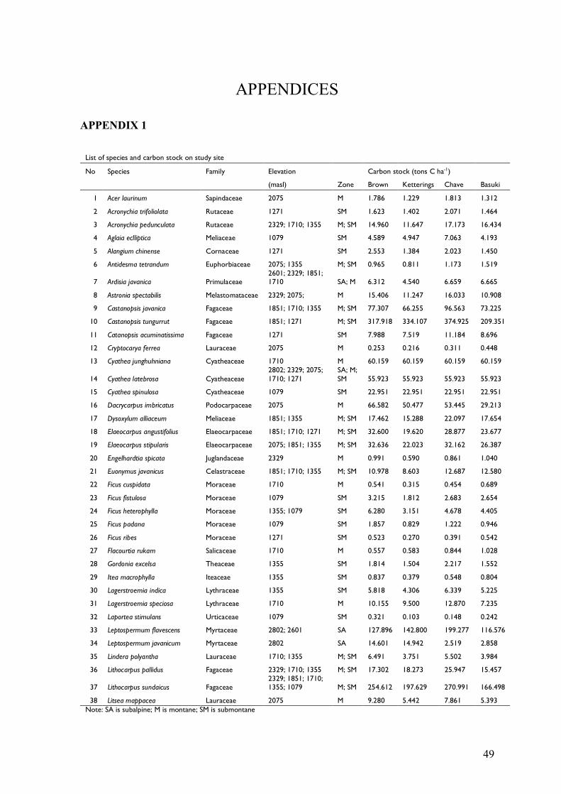
49

APPENDICES

APPENDIX 1

List of species and carbon stock on study site

No Species Family Elevation Carbon stock (tons C ha-1)

(masl) Zone Brown Ketterings Chave Basuki

1 Acer laurinum Sapindaceae 2075 M 1.786 1.229 1.813 1.312

2 Acronychia trifoliolata Rutaceae 1271 SM 1.623 1.402 2.071 1.464

3 Acronychia pedunculata Rutaceae 2329; 1710; 1355 M; SM 14.960 11.647 17.173 16.434

4 Aglaia eclliptica Meliaceae 1079 SM 4.589 4.947 7.063 4.193

5 Alangium chinense Cornaceae 1271 SM 2.553 1.384 2.023 1.450

6 Antidesma tetrandum Euphorbiaceae 2075; 1355 M; SM 0.965 0.811 1.173 1.519

7 Ardisia javanica Primulaceae 2601; 2329; 1851; 1710 SA; M 6.312 4.540 6.659 6.665

8 Astronia spectabilis Melastomataceae 2329; 2075; M 15.406 11.247 16.033 10.908

9 Castanopsis javanica Fagaceae 1851; 1710; 1355 M; SM 77.307 66.255 96.563 73.225

10 Castanopsis tungurrut Fagaceae 1851; 1271 M; SM 317.918 334.107 374.925 209.351

11 Catanopsis acuminatissima Fagaceae 1271 SM 7.988 7.519 11.184 8.696

12 Cryptocarya ferrea Lauraceae 2075 M 0.253 0.216 0.311 0.448

13 Cyathea junghuhniana Cyatheaceae 1710 M 60.159 60.159 60.159 60.159

14 Cyathea latebrosa Cyatheaceae 2802; 2329; 2075; 1710; 1271

SA; M; SM 55.923 55.923 55.923 55.923

15 Cyathea spinulosa Cyatheaceae 1079 SM 22.951 22.951 22.951 22.951

16 Dacrycarpus imbricatus Podocarpaceae 2075 M 66.582 50.477 53.445 29.213

17 Dysoxylum alliaceum Meliaceae 1851; 1355 M; SM 17.462 15.288 22.097 17.654

18 Elaeocarpus angustifolius Elaeocarpaceae 1851; 1710; 1271 M; SM 32.600 19.620 28.877 23.677

19 Elaeocarpus stipularis Elaeocarpaceae 2075; 1851; 1355 M; SM 32.636 22.023 32.162 26.387

20 Engelhardtia spicata Juglandaceae 2329 M 0.991 0.590 0.861 1.040

21 Euonymus javanicus Celastraceae 1851; 1710; 1355 M; SM 10.978 8.603 12.687 12.580

22 Ficus cuspidata Moraceae 1710 M 0.541 0.315 0.454 0.689

23 Ficus fistulosa Moraceae 1079 SM 3.215 1.812 2.683 2.654

24 Ficus heterophylla Moraceae 1355; 1079 SM 6.280 3.151 4.678 4.405

25 Ficus padana Moraceae 1079 SM 1.857 0.829 1.222 0.946

26 Ficus ribes Moraceae 1271 SM 0.523 0.270 0.391 0.542

27 Flacourtia rukam Salicaceae 1710 M 0.557 0.583 0.844 1.028

28 Gordonia excelsa Theaceae 1355 SM 1.814 1.504 2.217 1.552

29 Itea macrophylla Iteaceae 1355 SM 0.837 0.379 0.548 0.804

30 Lagerstroemia indica Lythraceae 1355 SM 5.818 4.306 6.339 5.225

31 Lagerstroemia speciosa Lythraceae 1710 M 10.155 9.500 12.870 7.235

32 Laportea stimulans Urticaceae 1079 SM 0.321 0.103 0.148 0.242

33 Leptospermum flavescens Myrtaceae 2802; 2601 SA 127.896 142.800 199.277 116.576

34 Leptospermum javanicum Myrtaceae 2802 SA 14.601 14.942 2.519 2.858

35 Lindera polyantha Lauraceae 1710; 1355 M; SM 6.491 3.751 5.502 3.984

36 Lithocarpus pallidus Fagaceae 2329; 1710; 1355 M; SM 17.302 18.273 25.947 15.457

37 Lithocarpus sundaicus Fagaceae 2329; 1851; 1710; 1355; 1079 M; SM 254.612 197.629 270.991 166.498

38 Litsea mappacea Lauraceae 2075 M 9.280 5.442 7.861 5.393 Note: SA is subalpine; M is montane; SM is submontane

50

APPENDIX 1 (continues)

List of species and carbon stock on study site No Species Family Elevation Zona Carbon stock (tons C ha-1)

(masl) Brown Ketterings Chave Basuki

39 Macropanax concinnus Araliaceae 2802; 1851; 1710 SA; M 16.549 7.786 11.525 11.560

40 Macropanax dispermum Araliaceae 2329; 2075; 1355 M; SM 22.346 10.475 15.491 15.773

41 Magnolia lilifera Magnoliaceae 1710 M 0.685 0.443 0.643 0.818

42 Myrsine hasseltii Primulaceae 2802; 2601; 2329; 1851

SA; M 93.943 85.970 126.022 104.398

43 Neolitsea cassiaefolia Lauraceae 2329; 2075; 1710; 1355

M; SM 79.146 71.690 101.100 64.969

44 Neolitsea javanica Lauraceae 2075; 1851; 1710; 1355

M; SM 47.880 40.409 59.087 43.484

45 Oreocnide scabra Urticaceae 1851; 1079 M; SM 27.434 18.874 27.820 27.296

46 Paraserianthes lophantha

Fabaceae 2601; 1710 SA; M 1.048 1.048 1.048 1.048

47 Phoebe grandis Lauraceae 1355 SM 6.992 4.176 6.207 5.479

48 Pinanga coronata Arecaceae 1079 SM 22.615 17.147 24.668 19.401

49 Platea latifolia Icacinaceae 2075; 1851; 1710 M 96.328 52.300 76.516 61.497

50 Polyosma integrifolia Escalloniaceae 2601; 2075; 1851; 1710

M 12.489 9.026 13.232 13.204

51 Prunus arborea Rosaceae 1355 SM 25.362 21.441 31.349 21.019

52 Rapanea hasseltii Primulaceae 1355 SM 2.110 2.083 3.061 2.037

53 Schima wallichii Theaceae 2601; 2329; 2075; 1851; 1710 ; 1355; 1271

SA; M; SM 652.434 581.317 772.624 451.682

54 Schefflera scandens Araliaceae 2601 SA 0.253 0.118 0.170 0.271

55 Symplocos odoratissima Symplocaceae 2802; 2601 SA 83.935 60.494 86.232 83.466

56 Syzygium antisepticum Myrtaceae 1710 M 12.412 9.830 13.086 7.448

57 Syzygium racemosum Myrtaceae 2075 M 23.934 28.824 40.316 22.747

58 Syzygium rostratum Myrtaceae 2075; 1851; 1710 M 38.506 44.741 65.349 48.864

59 Toona sureni Meliaceae 1079 SM 91.688 52.428 52.134 30.180

60 Trema orientalis Cannabaceae 1271; 1079 SM 14.729 7.713 10.605 6.796

61 Turpinia sphaerocarpa Staphyleaceae 1710 M 0.873 0.439 0.634 0.911

62 Urophyllum arboreum Rubiaceae 1851; 1355 M; SM 1.464 0.803 1.169 1.480

63 Vaccinium varingiaefolium

Ericaceae 2802; 2601 SA 379.925 361.938 514.088 346.264

64 Vernonia arborea Asteraceae 2329 M 27.969 14.537 21.443 17.753

65 Weinmannia blumei Cunoniaceae 1710 M 4.184 3.469 5.149 4.560

66 Ziziphus angustifolia Rhamnaceae 1355 SM 0.232 0.196 0.283 0.414

Note: SA is subalpine; M is montane; SM is submontane

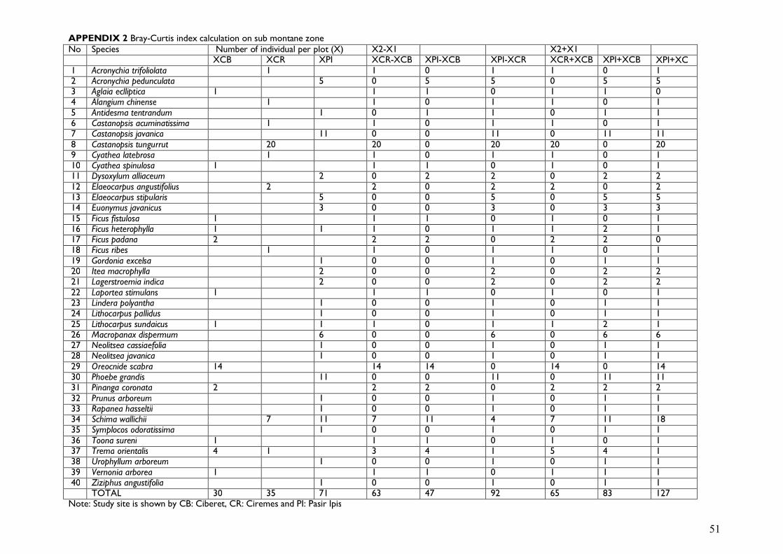
51

APPENDIX 2 Bray-Curtis index calculation on sub montane zone No Species Number of individual per plot (X) X2-X1 X2+X1 XCB XCR XPI XCR-XCB XPI-XCB XPI-XCR XCR+XCB XPI+XCB XPI+XC

R 1 Acronychia trifoliolata 1 1 0 1 1 0 1 2 Acronychia pedunculata 5 0 5 5 0 5 5 3 Aglaia eclliptica 1 1 1 0 1 1 0 4 Alangium chinense 1 1 0 1 1 0 1 5 Antidesma tentrandum 1 0 1 1 0 1 1 6 Castanopsis acuminatissima 1 1 0 1 1 0 1 7 Castanopsis javanica 11 0 0 11 0 11 11 8 Castanopsis tungurrut 20 20 0 20 20 0 20 9 Cyathea latebrosa 1 1 0 1 1 0 1 10 Cyathea spinulosa 1 1 1 0 1 0 1 11 Dysoxylum alliaceum 2 0 2 2 0 2 2 12 Elaeocarpus angustifolius 2 2 0 2 2 0 2 13 Elaeocarpus stipularis 5 0 0 5 0 5 5 14 Euonymus javanicus 3 0 0 3 0 3 3 15 Ficus fistulosa 1 1 1 0 1 0 1 16 Ficus heterophylla 1 1 1 0 1 1 2 1 17 Ficus padana 2 2 2 0 2 2 0 18 Ficus ribes 1 1 0 1 1 0 1 19 Gordonia excelsa 1 0 0 1 0 1 1 20 Itea macrophylla 2 0 0 2 0 2 2 21 Lagerstroemia indica 2 0 0 2 0 2 2 22 Laportea stimulans 1 1 1 0 1 0 1 23 Lindera polyantha 1 0 0 1 0 1 1 24 Lithocarpus pallidus 1 0 0 1 0 1 1 25 Lithocarpus sundaicus 1 1 1 0 1 1 2 1 26 Macropanax dispermum 6 0 0 6 0 6 6 27 Neolitsea cassiaefolia 1 0 0 1 0 1 1 28 Neolitsea javanica 1 0 0 1 0 1 1 29 Oreocnide scabra 14 14 14 0 14 0 14 30 Phoebe grandis 11 0 0 11 0 11 11 31 Pinanga coronata 2 2 2 0 2 2 2 32 Prunus arboreum 1 0 0 1 0 1 1 33 Rapanea hasseltii 1 0 0 1 0 1 1 34 Schima wallichii 7 11 7 11 4 7 11 18 35 Symplocos odoratissima 1 0 0 1 0 1 1 36 Toona sureni 1 1 1 0 1 0 1 37 Trema orientalis 4 1 3 4 1 5 4 1 38 Urophyllum arboreum 1 0 0 1 0 1 1 39 Vernonia arborea 1 1 1 0 1 1 1 40 Ziziphus angustifolia 1 0 0 1 0 1 1

TOTAL 30 35 71 63 47 92 65 83 127 Note: Study site is shown by CB: Ciberet, CR: Ciremes and PI: Pasir Ipis

52

APPENDIX 2 (continues) Bray-Curtis index calculation on montane zone Number of individual

per plot (X) X2-X1 X2+X1

XSB XSB XSB XSB XSBIII- XSBIV- XSBV-

XSBIV- XSBV-

XSBV-

XSBIII+ XSBIV+ XSBV+ XSBIV+ XSBV+

XSBV+ No Species II III IV V XSBII XSBII XSBII XSBIII XSBII

I XSBIV

XSBII XSBII XSBII XSBIII XSBIII

XSBIV 1 Acer laurinum 1 1 0 0 1 1 0 1 0 0 1 1 0 2 Acronychia pedunculata 9 1 9 9 8 0 1 1 9 9 10 0 1 1 3 Antidesma tetrandum 1 1 0 0 1 1 0 1 0 0 1 1 0 4 Ardisia javanica 1 3 2 1 2 1 3 2 1 1 4 3 3 2 5 5 Astronia spectabilis 2 4 2 2 2 4 4 0 6 2 2 4 4 0 6 Castanopsis javanica 7 3 0 7 3 7 3 4 0 7 3 7 3 10 7 Castanopsis tungurrut 7 0 7 0 7 0 7 0 7 0 7 0 7 8 Cryptocarya ferrea 1 1 0 0 1 1 0 1 0 0 1 1 0 9 Cyathea junghuniana 4 0 0 4 0 4 4 0 0 4 0 4 4

10 Cyathea latebrosa 2 2 5 0 2 3 2 3 5 4 2 7 2 7 5 11 Dacrycarpus imbricatus 1 1 0 0 1 1 0 1 0 0 1 1 0 12 Dysoxylum alliaceum 5 0 5 0 5 0 5 0 5 0 5 0 5 13 Elaeocarpus angustifolius 7 6 0 7 6 7 6 1 0 7 6 7 6 13 14 Elaeocarpus stipularis 1 6 1 6 0 5 1 6 1 6 0 7 1 6 15 Engelhardtia spicata 1 1 1 1 0 0 0 1 1 1 0 0 0 16 Euonymus javanicus 1 7 0 1 7 1 7 6 0 1 7 1 7 8 17 Ficus cuspidata 8 0 0 8 0 8 8 0 0 8 0 8 8 18 Flaucortia rukam 9 0 0 9 0 9 9 0 0 9 0 9 9 19 Lagerstroemia speciosa 1 0 0 1 0 1 1 0 0 1 0 1 1 20 Lindera polyantha 2 0 0 2 0 2 2 0 0 2 0 2 2 21 Lithocarpus pallidus 1 2 1 1 1 0 2 2 1 1 3 0 2 2 22 Lithocarpus sundaicus 15 2 7 15 13 8 2 7 5 15 17 22 2 7 9 23 Litsea mappacea 3 3 0 0 3 3 0 3 0 0 3 3 0 24 Macropanax concinnus 2 5 0 2 5 2 5 3 0 2 5 2 5 7 25 Macropanax dispermum 3 3 0 3 3 3 3 0 6 3 3 3 3 0 26 Magnolia lilifera 1 0 0 1 0 1 1 0 0 1 0 1 1 27 Myrsine hasseltii 1 1 1 0 1 1 0 1 1 2 1 1 0 1 28 Neolitsea cassiaefolia 5 1 5 4 5 0 1 4 5 6 5 10 1 6 5 29 Neolitsea javanica 13 1 6 13 1 6 12 7 5 13 1 6 14 19 7 30 Oreocnide scabra 1 0 1 0 1 0 1 0 1 0 1 0 1 31 Paraserianthes lophanta 1 0 0 1 0 1 1 0 0 1 0 1 1 32 Platea latifolia 16 4 3 16 4 3 12 13 1 16 4 3 20 19 7 33 Polyosma integrifolia 7 2 1 7 2 1 5 6 1 7 2 1 9 8 3 34 Schima wallichii 20 12 12 14 8 8 6 0 2 2 32 32 34 24 26 26 35 Syzygium antisepticum 1 0 0 1 0 1 1 0 0 1 0 1 1 36 Syzygium racemosum 3 3 0 0 3 3 0 3 0 0 3 3 0 37 Syzygium rostratum 2 8 2 2 8 2 6 0 6 2 8 8 10 4 10 38 Turpinia sphaerocarpa 2 0 0 2 0 2 2 0 0 2 0 2 2 39 Urophyllum arboreum 1 0 1 0 1 0 1 0 1 0 1 0 1 40 Vernonia arborea 10 10 10 10 0 0 0 10 10 10 0 0 0 41 Weinmannia blumei 1 0 0 1 0 1 1 0 0 1 0 1 1

TOTAL 70 71 70 99 101 108 107 97 116 99 141 140 175 141 170 169 Note: Study site is shown by SB II-V: Selabintana II-V

53

APPENDIX 2 (continues)

Bray-Curtis index calculation on subalpine zone

Number of individual per plot X2-X1 X2+X1

No Species XGM XSBI XSBI-XGM XSBI+XGM

1 Ardisia javanica 1 1 1

2 Cyathea latebrosa 1 1 1

3 Leptospermum flavescens 4 23 19 27

4 Leptospermum javanicum 3 3 3

5 Macropanax concinnus 2 2 2

6 Myrsine hasseltii 29 26 3 55

7 Paraserianthes lophanta 1 1 1

8 Polyosma integrifolia 1 1 1

9 Schima wallichii 2 2 2

10 Schleffera scandens 1 1 1

11 Symplocos odoratissima 29 19 10 48

12 Vaccinium varingiaefolium 41 40 1 81

TOTAL 109 114 45 223

Note: Study site is shown by GM: Gunung Gemuruh, SB I: Selabintana I

54

APPENDIX 3

Shannon Index, number of species and highest importance value on study site

Note: * is maximum value and ^ is minimum value

Site

Elevation (masl)

Zone

Number of species

Shannon Index

Highest importance value

Gunung 2802 Sub Alpin 7 1.409^ Vaccinium varingiaefolium 121.215

Gemuruh Myrsine hasseltii 36.301

Symplocos odoratissima 32.797

Selabintana I 2601 Sub Alpin 9 1.563 Vaccinium varingiaefolium 89.940

Leptospermum flavescens 56.172

Myrsine hasseltii 29.784

Selabintana II 2329 Montana 12 1.999 Schima wallichii 81.774

Lithocarpus sundaicus 59.069

Vernonia arborea 21.274

Selabintana III 2075 Montana 16 2.300 Schima wallichii 64.538

Platea latifolia 49.593

Neolitsea javanica 33.273

Selabintana IV 1851 Montana 17 2.547 Schima wallichii 53.363

Castanopsis tungurrut 32.369

Castanopsis javanica 20.593

Selabintana V 1710 Montana 25 2.925* Schima wallichii 91.645

Lithocarpus sundaicus 22.046

PasirIpis 1355 Sub Montana

23 2.701 Schima wallichii 42.386

Phoebe grandis 24.987

Castanopsis javanica 20.191

Ciremes 1271 Sub Montana

9 1.415 Castanopsis acuminatissima 95.206

Castanopsis tungurrut 57.179

Schima wallichii 27.067

Ciberet 1079 Sub Montana

12 1.892 Oreocnide scabra 78.753

Trema orientalis 52.014

Toona sureni 23.138

55

APPENDIX 4

Species density at the observation plots on Mount Gede Pangrango National Park Species Density Species Density

(individuals ha-1) (individuals ha-1)

Vaccinium varingiaefolium 405 Lindera polyantha 15 Schima wallichii 390 Litsea mappacea 15

Myrsine hasseltii 285 Syzygium racemosum 15

Symplocos odoratissima 245 Antidesma tetrandum 10

Castanopsis tungurrut 135 Ficus heterophylla 10

Leptospermum flavescens 135 Ficus padana 10

Lithocarpus sundaicus 125 Itea macrophylla 10

Platea latifolia 115 Lagerstroemia indica 10

Castanopsis javanica 105 Paraserianthes lophanta 10

Neolitsea javanica 105 Pinanga coronata 10

Elaeocarpus angustifolius 75 Turpinia sphaerocarpa 10

Oreocnide scabra 75 Urophyllum arboreum 10

Elaeocarpus stipularis 60 Acer laurinum 5

Macropanax dispermum 60 Acronychia trifoliolata 5

Neolitsea cassiaefolia 60 Aglaia eclliptica 5

Syzygium rostratum 60 Alangium chinense 5

Cyathea latebrosa 55 Cryptocarya ferrea 5

Euonymus javanicus 55 Cyathea spinulosa 5

Phoebe grandis 55 Dacrycarpus imbricatus 5

Polyosma integrifolia 55 Engelhardtia spicata 5

Vernonia arborea 55 Ficus fistulosa 5

Flacourtia rukam 45 Ficus ribes 5

Macropanax concinnus 45 Gordonia excelsa 5

Ficus cuspidata 40 Lagerstroemia speciosa 5

Ardisia javanica 35 Laportea stimulans 5

Dysoxylum alliaceum 35 Magnolia lilifera 5

Astronia spectabilis 30 Prunus arborea 5

Trema orientalis 25 Rapanea hasseltii 5

Cyathea junghuhniana 20 Schefflera scandens 5

Lithocarpus pallidus 20 Syzygium antisepticum 5

Catanopsis acuminatissima 20 Toona sureni 5

Acronychia pedunculata 15 Weinmannia blumei 5

Leptospermum javanicum 15 Ziziphus angustifolia 5

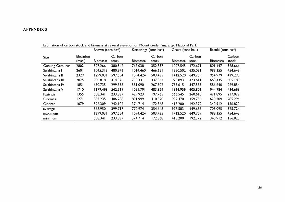
56

APPENDIX 5

Estimation of carbon stock and biomass at several elevation on Mount Gede Pangrango National Park

Site Elevation (masl)

Brown (tons ha-1)

Ketterings (tons ha-1)

Chave (tons ha-1)

Basuki (tons ha-1)

Biomassa Carbon stock Biomassa

Carbon stock Biomassa

Carbon stock Biomassa

Carbon stock

Gunung Gemuruh 2802 827.266 380.542 767.038 352.837 1027.545 472.671 801.447 368.666

Selabintana I 2601 1045.318 480.846 1014.460 466.651 1380.502 635.031 988.355 454.643

Selabintana II 2329 1299.031 597.554 1094.424 503.435 1412.520 649.759 954.979 439.290

Selabintana III 2075 900.818 414.376 733.331 337.332 920.893 423.611 663.435 305.180

Selabintana IV 1851 650.735 299.338 581.090 267.302 755.615 347.583 586.640 269.854

Selabintana V 1710 1179.498 542.569 1051.791 483.824 1316.959 605.801 944.984 434.693

PasirIpis 1355 508.341 233.837 429.923 197.765 566.545 260.610 471.895 217.072

Ciremes 1271 883.235 406.288 891.999 410.320 999.470 459.756 620.209 285.296

Ciberet 1079 526.309 242.102 374.714 172.368 418.200 192.372 340.912 156.820

average 868.950 399.717 770.974 354.648 977.583 449.688 708.095 325.724

maximum 1299.031 597.554 1094.424 503.435 1412.520 649.759 988.355 454.643

minimum 508.341 233.837 374.714 172.368 418.200 192.372 340.912 156.820

57

APPENDIX 6

Aboveground and soil carbon stock on study site

Aboveground biomass

Contribution

Soil carbon Contribution Total carbon stock

Site Elevation (tons ha-1) (%) (tons C ha-1) (%) (tons C ha-1)

(masl) Brown Ketterings Chave Basuki Brown Ketterings Chave Basuki Brown Ketterings Chave Basuki

Gunung Gemuruh 2802 380.542 352.837 472.671 368.666 99.998 99.998 99.999 99.998 0.007 0.002 380.549 352.844 472.677 368.672

Selabintana I 2601 480.846 466.651 635.031 454.643 99.998 99.998 99.999 99.998 0.007 0.001 480.854 466.659 635.038 454.651

Selabintana II 2329 597.554 503.435 649.759 439.29 99.999 99.999 99.999 99.999 0.006 0.001 597.56 503.441 649.765 439.296

Selabintana III 2075 414.376 337.332 423.611 305.18 99.998 99.998 99.998 99.998 0.007 0.002 414.383 337.339 423.618 305.187

Selabintana IV 1851 299.338 267.302 347.583 269.854 99.998 99.997 99.998 99.997 0.007 0.002 299.345 267.309 347.59 269.861

Selabintana V 1710 542.569 483.824 605.801 434.693 99.999 99.999 99.999 99.999 0.006 0.001 542.575 483.83 605.807 434.699

PasirIpis 1355 233.837 197.765 260.61 217.072 99.998 99.997 99.998 99.997 0.006 0.003 233.843 197.77 260.616 217.077

Ciremes 1271 406.288 410.32 459.756 285.296 99.999 99.999 100.000 99.999 0.002 0.001 406.29 410.322 459.758 285.298

Ciberet 1079 242.102 172.368 192.372 156.82 99.996 99.994 99.994 99.993 0.011 0.006 242.113 172.379 192.383 156.83

average 399.717 354.648 449.688 325.724 350.7095 338.0156 325.3217 312.6278 0.007 0.002 399.724 354.655 449.695 325.73

maximum 597.554 503.435 649.759 454.643 480.7455 452.5046 424.2637 396.0228 0.007 0.003 597.56 503.441 649.765 454.651

minimum 233.837 197.765 260.61 217.072 230.4585 231.7135 232.9685 234.2235 0.002 0.001 233.843 197.77 260.616 217.077

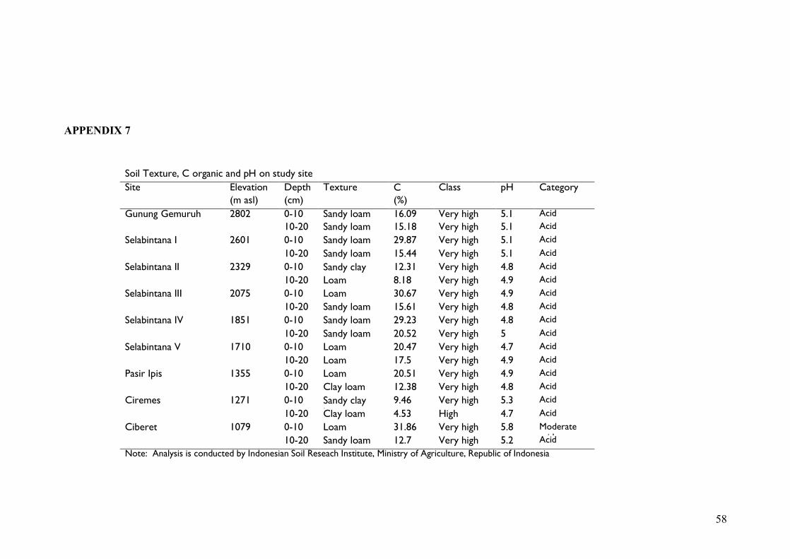
58

APPENDIX 7

Soil Texture, C organic and pH on study site

Site Elevation Depth Texture C organic

Class pH Category (m asl) (cm) (%)

Gunung Gemuruh 2802 0-10 Sandy loam 16.09 Very high 5.1 Acid

10-20 Sandy loam 15.18 Very high 5.1 Acid

Selabintana I 2601 0-10 Sandy loam 29.87 Very high 5.1 Acid


Selabintana II 2329 0-10 Sandy clay loam

12.31 Very high 4.8 Acid

10-20 Loam 8.18 Very high 4.9 Acid

Selabintana III 2075 0-10 Loam 30.67 Very high 4.9 Acid


Selabintana IV 1851 0-10 Sandy loam 29.23 Very high 4.8 Acid

10-20 Sandy loam 20.52 Very high 5 Acid

Selabintana V 1710 0-10 Loam 20.47 Very high 4.7 Acid

10-20 Loam 17.5 Very high 4.9 Acid

Pasir Ipis 1355 0-10 Loam 20.51 Very high 4.9 Acid

10-20 Clay loam 12.38 Very high 4.8 Acid

Ciremes 1271 0-10 Sandy clay loam

9.46 Very high 5.3 Acid

10-20 Clay loam 4.53 High 4.7 Acid

Ciberet 1079 0-10 Loam 31.86 Very high 5.8 Moderate acid 10-20 Sandy loam 12.7 Very high 5.2 Acid

Note: Analysis is conducted by Indonesian Soil Reseach Institute, Ministry of Agriculture, Republic of Indonesia

59

APPENDIX 8

Microclimate on study site

Elevation Slope Temperature (C) Relative humidity (%)

Soil moisture

Site (masl) (%) Max Min Max Min (%)

Gunung Gemuruh 2802 67.5 23.8 15.6 53 36 47.3

Selabintana I 2601 65 23.8 8.4 64 36 54.5

Selabintana II 2329 52 23.8 8.4 69.3 36 67.3

Selabintana III 2075 44 23.8 10.9 76.5 45.8 55.3

Selabintana IV 1851 26 24.8 17.8 78 60 54

Selabintana V 1710 35 24.8 17.7 89 60 50

Pasir Ipis 1355 35 24.8 17.7 89.8 60 58

Ciremes 1271 33 22* 18* 90* 80* 47.13

Ciberet 1079 13 22* 18* 90* 80* 67.6 *: Mount Gede Pangrango National Park (2011)