achim j. lilienthal130.243.105.49/research/learning/courses/dip/2011/lectures/dip_2011_l05.pdf ·...
TRANSCRIPT

Achim J. LilienthalAASS Learning Systems Lab, Örebro University

2 2D Illustration
qp
output input
� � � ���
���S
IIIGGW
IBFq
qqpp
p qp ||||||1][rs ��
p
reproduced from [Durand 02]

2 1D Illustration
� Space and Range Parameters
� space �s : spatial extent of the kernel, size of the considered neighborhood
� range �r : "minimum" amplitude of an edge
� � � ���
���S
IIIGGW
IBFq
qqpp
p qp ||||||1][rs ��

2 Bilateral Filtering
� Space and Range Parameters
p
space
range
consider only pixels close in space and similar in range!

2 Bilateral Filtering
� Space and Range Parameters� ...
�s = 2
�s = 6
�r = 0.1 �r = 0.25�r =
(Gaussian blur)
input

2 Bilateral Filtering
� Space and Range Parameters� ...
�r = 0.1 �r = 0.25�r =
(Gaussian blur)
input
�s = 18
�s = 6

2 Bilateral Filtering
� Varying the Range Parameter� ...
�s = 2
�s = 6
�r = 0.1 �r = 0.25�r =
(Gaussian blur)
input
1 Spatial Filtering5 input
from "A Gentle Introduction to Bilateral Filtering and its Applications", S. Paris, P. Kornprobst, J. Tumblin, and F. Durand, SIGGRAPH 2008

1 Spatial Filtering5 input�r = 0.1
from "A Gentle Introduction to Bilateral Filtering and its Applications", S. Paris, P. Kornprobst, J. Tumblin, and F. Durand, SIGGRAPH 2008

1 Spatial Filtering5 �r = 0.25
from "A Gentle Introduction to Bilateral Filtering and its Applications", S. Paris, P. Kornprobst, J. Tumblin, and F. Durand, SIGGRAPH 2008

1 Spatial Filtering5 �r = (Gaussian blur)
from "A Gentle Introduction to Bilateral Filtering and its Applications", S. Paris, P. Kornprobst, J. Tumblin, and F. Durand, SIGGRAPH 2008

2 Bilateral Filtering
� Varying the Space Parameter� ...
�s = 6
�r = 0.1 �r = 0.25�r =
(Gaussian blur)
input
�s = 18ssssssssssssss 18
�s = 2

1 Spatial Filtering5 input
from "A Gentle Introduction to Bilateral Filtering and its Applications", S. Paris, P. Kornprobst, J. Tumblin, and F. Durand, SIGGRAPH 2008

1 Spatial Filtering5 �s = 2
from "A Gentle Introduction to Bilateral Filtering and its Applications", S. Paris, P. Kornprobst, J. Tumblin, and F. Durand, SIGGRAPH 2008

1 Spatial Filtering5 �s = 6
from "A Gentle Introduction to Bilateral Filtering and its Applications", S. Paris, P. Kornprobst, J. Tumblin, and F. Durand, SIGGRAPH 2008

1 Spatial Filtering5 �s = 18
from "A Gentle Introduction to Bilateral Filtering and its Applications", S. Paris, P. Kornprobst, J. Tumblin, and F. Durand, SIGGRAPH 2008

2 Bilateral Filtering
� How to Set the Parameters?� depends on the application, for instance …
� space parameter: proportional to image size� e.g.: 2% of image diagonal
� range parameter: proportional to edge amplitude� e.g.: mean or median of image gradients (MAD)
� independent of resolution and exposure

2 Bilateral Filtering
� A 3rd Parameter – Iterating Bilateral Filtering
� generates more piecewise-flat images
][ )()1( nn IBFI �

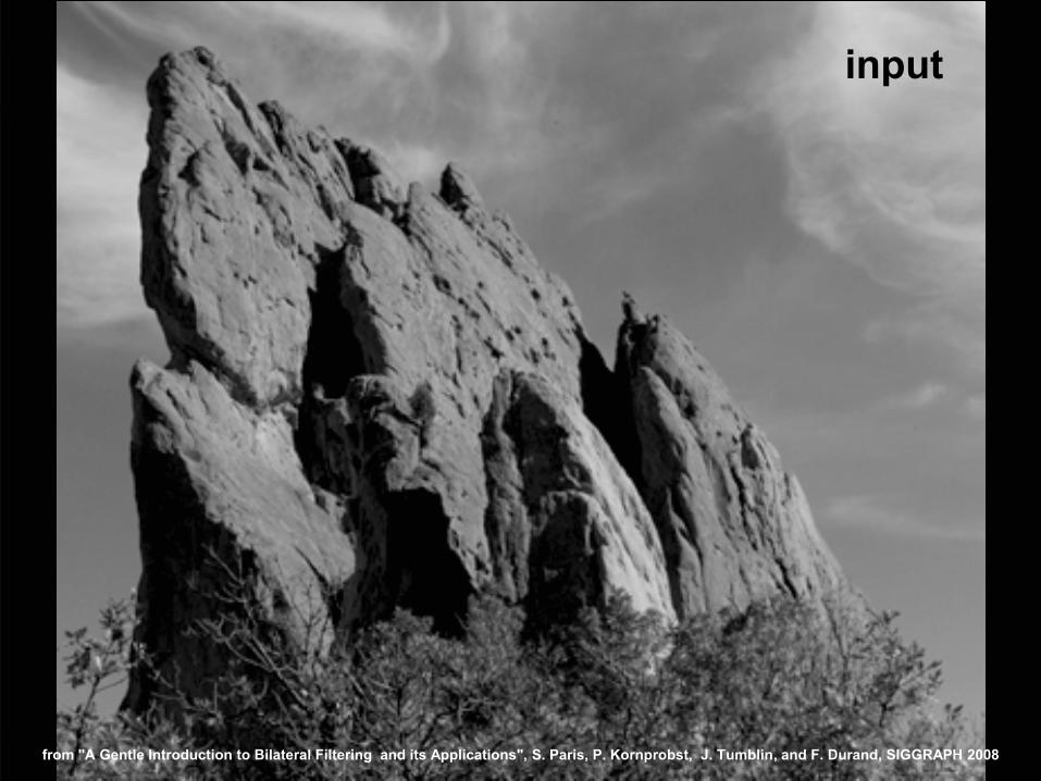
1 Spatial Filtering5 input
from "A Gentle Introduction to Bilateral Filtering and its Applications", S. Paris, P. Kornprobst, J. Tumblin, and F. Durand, SIGGRAPH 2008

1 Spatial Filtering5 iteration 1
from "A Gentle Introduction to Bilateral Filtering and its Applications", S. Paris, P. Kornprobst, J. Tumblin, and F. Durand, SIGGRAPH 2008
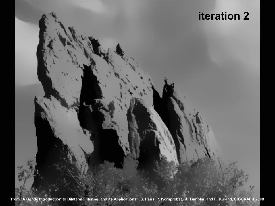
1 Spatial Filtering5 iteration 2
from "A Gentle Introduction to Bilateral Filtering and its Applications", S. Paris, P. Kornprobst, J. Tumblin, and F. Durand, SIGGRAPH 2008

1 Spatial Filtering5 iteration 4
from "A Gentle Introduction to Bilateral Filtering and its Applications", S. Paris, P. Kornprobst, J. Tumblin, and F. Durand, SIGGRAPH 2008

2 Bilateral Filtering
� Remarks� bilateral filter is nonlinear
� complex, spatially varying kernels� cannot be pre-computed, no FFT…
� � � ���
���S
IIIGGW
IBFq
qqpp
p qp ||||||1][rs ��

2 Bilateral Filtering
� Bilateral Filtering Color Images
� � � ���
���S
IIIGGW
IBFq
qqpp
p qp ||||||1][rs ��
For gray-level images intensity difference
scalar
input
output

2 Bilateral Filtering
� Bilateral Filtering Color Images
� best done in a "perceptual color space" (CIE-Lab, HSI)� where Euclidean distance corresponds to human color discrimination
� � � ���
���S
IIIGGW
IBFq
qqpp
p qp ||||||1][rs ��
� � � ���
���S
GGW
IBFq
qqpp
p CCCqp ||||||||1][rs ��
For gray-level images
For color images
intensity difference
color difference
scalar
3D vector (RGB, L*a*b*, …)
input
output

Agenda
Applications of Bilateral Filtering
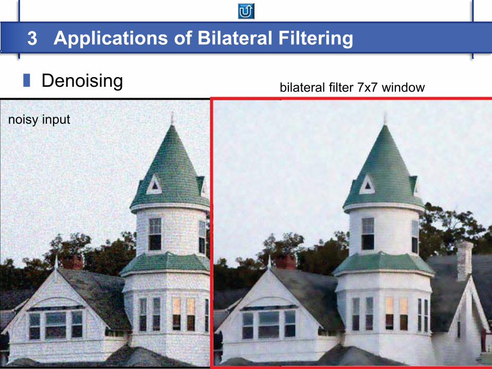
3 Applications of Bilateral Filtering
� Denoising� ...
noisy input
bilateral filter 7x7 window

3 Applications of Bilateral Filtering
� Denoising� ...
noisy input
median 3x3
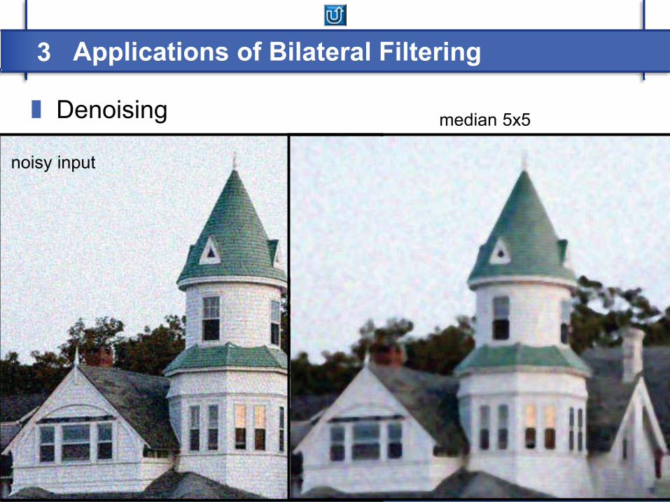
3 Applications of Bilateral Filtering
� Denoising� ...
noisy input
median 5x5

3 Applications of Bilateral Filtering
� Denoising� ...
noisy input
bilateral filter 7x7 window, lower �

3 Applications of Bilateral Filtering
� Denoising� ...
noisy input
bilateral filter 7x7 window, higher �

3 Applications of Bilateral Filtering
� Denoising� small spatial sigma (e.g. 7x7 window)
� adapt range sigma to noise level
� maybe not best denoising method, but best simplicity/quality trade-off
� no need for acceleration (small kernel)

3 Applications of Bilateral Filtering
� Large-Scale/Small-Scale Decomposition
input smoothed(structure, large scale)
residual(texture, small scale)
3 Applications of Bilateral Filtering
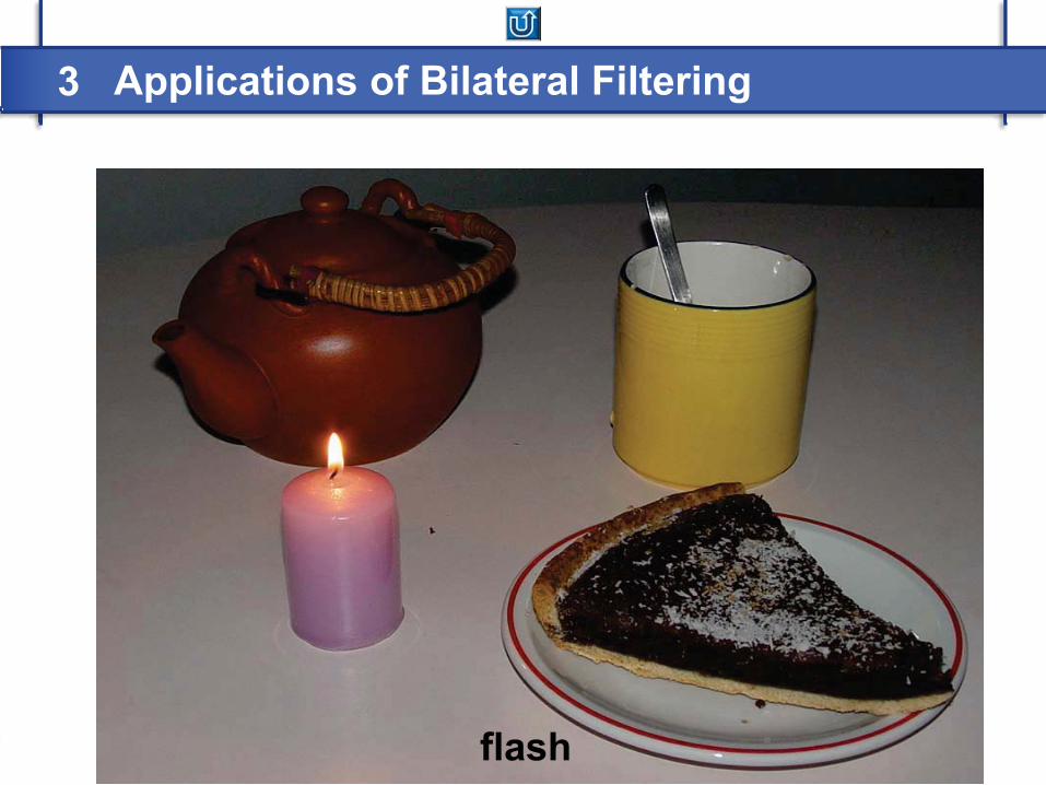
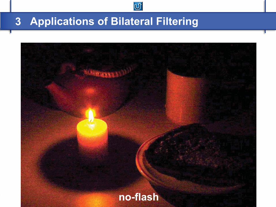
� Flash/No-Flash Photo Improvement� intensities from no-flash image
� noisy
� dim
� compute range kernel on flash image� clean
� cross bilateral filter (also "joint bilateral filter")

3 Applications of Bilateral Filtering
no-flash
3 Applications of Bilateral Filtering
flash

3 Applications of Bilateral Filtering
cross bilateral filtered
3 Applications of Bilateral Filtering
no-flash

3 Applications of Bilateral Filtering
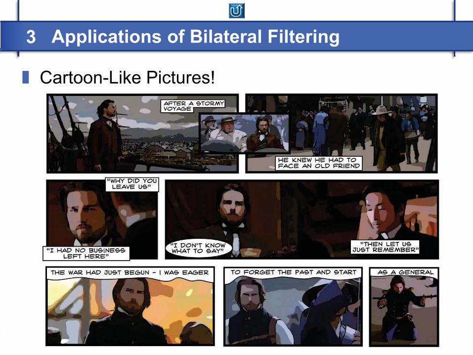
� Cartoon-Like Pictures� [Winnemöller, Olsen, Gooch, 2006]
input output
3 Applications of Bilateral Filtering
� Cartoon-Like Pictures!

3 Applications of Bilateral Filtering
� Cartoon-Like Pictures – Not Straightforward!� [Winnemöller, Olsen, Gooch, 2006]

3 Applications of Bilateral Filtering
� Cartoon-Like Pictures – Implementation Available!

3 Applications of Bilateral Filtering
� Video Enhancement� extend bilateral filter to time domain

3 Applications of Bilateral Filtering
� Video Enhancement [AVI]
see http://ericpbennett.com/VideoEnhancement/index.htm

3 Applications of Bilateral Filtering
� Further Applications� image simplification
� bilateral up-sampling
� mesh smoothing (3D extension)
� and ... many more
� Modifications and Extensions� use metrics different from "Gaussian of Euclidean"
� use oriented filters (oriented along image structures)
� ...

Agenda
Efficient Implementation
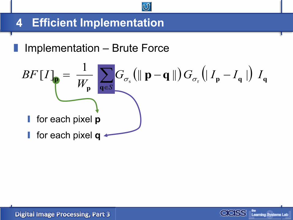
4 Efficient Implementation
� Implementation – Brute Force
� for each pixel p� for each pixel q
� � � ���
���S
IIIGGW
IBFq
qqpp
p qp ||||||1][rs ��

4 Efficient Implementation
� Implementation – Brute Force
� for each pixel p� for each pixel q� compute
� � � ���
���S
IIIGGW
IBFq
qqpp
p qp ||||||1][rs ��
� � � � qqpqp IIIGG ||||||rs
�� ��

4 Efficient Implementation
� Implementation – Brute Force
� for each pixel p� for each pixel q� compute
� � brute-force implementation is slow (O[(#pixels)2])� 8 megapixel photo � 64'000'000'000'000 iterations!
� � � ���
���S
IIIGGW
IBFq
qqpp
p qp ||||||1][rs ��
� � � � qqpqp IIIGG ||||||rs
�� ��

4 Efficient Implementation
� Implementation – Neglect Regions Far Away� for each pixel p evaluate pixels q in local neighbourhood
� � complexity (O[(#pixels � �S) ])� fast for small kernels
looking at all pixels looking at neighbors only

4 Efficient Implementation
� Implementation – More� pre-compute range kernel values
� separable kernel (approximation)
2011-04-14
DDigital Image Processing
Achim J. Lilienthal
AASS Learning Systems Lab, Dep. Teknik
Room T1209 (Fr, 11-12 o'clock)
Digital Image ProcessingPart 3: Fourier Transform and
Filtering in the Frequency Domain
Course Book Chapter 4

Achim J. Lilienthal
Discrete Fourier Transform
� Contents� Contents

Achim J. Lilienthal
Fourier Transform1
� Key idea (Fourier, 1807)� represent periodic functions as a weighted sum of sines

Achim J. Lilienthal
� Fourier Transform F� periodic functions f
� f � F = weighted sum of sines
� non-periodic functions f (with a finite integral)� f � F = integral of sines multiplied with a weighing function
� f can be reconstructed from F without loss of information
� Standard "Filtering in the Frequency Domain" Procedure� calculate the Fourier Transform F
� process the representation F "in the Fourier domain"
� return to the original domain
Fourier Transform1

Achim J. Lilienthal
� Discrete Fourier Transform DFT� consider a repeated part of a periodic function
Discrete Fourier Transform1

Achim J. Lilienthal
� Fourier Transform� consider a repeated part of a periodic function
Fourier Transform1

Achim J. Lilienthal
)0.2sin(2.11 xf �
Fourier Transform1

Achim J. Lilienthal
)10/0.4sin(45.02 � � xf
Fourier Transform1
Achim J. Lilienthal
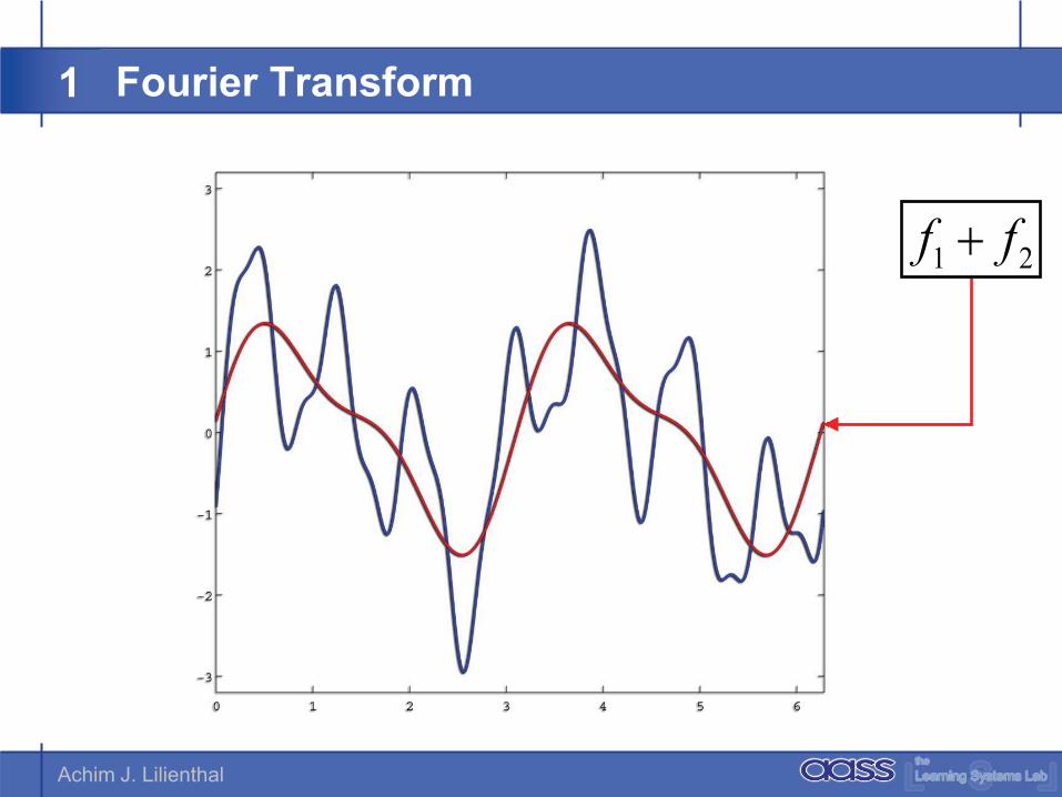
21 ff
Fourier Transform1

Achim J. Lilienthal
21 ff
)4/70.7sin(16.13 � � xf
Fourier Transform1

Achim J. Lilienthal
321 fff
Fourier Transform1

Achim J. Lilienthal
)7/120.17sin(3.04 � � xf
321 fff
Fourier Transform1

Achim J. Lilienthal
4321 ffff
Discrete Fourier Transform1

Achim J. Lilienthal
� 1D Discrete Fourier Transform� spatial domain
� signal as a weighted sum of box functions at the pixel locations
� box functions provide a convenient base of a vector space
� image as an element of a high-dimensional vector space
� intensity values are coefficients with respect to this base
� frequency domain� base is now a set of sinusoids
� coefficients indicate spatial frequency components
� Fourier transform� formalism to change the base
Discrete Fourier Transform1
Achim J. Lilienthal
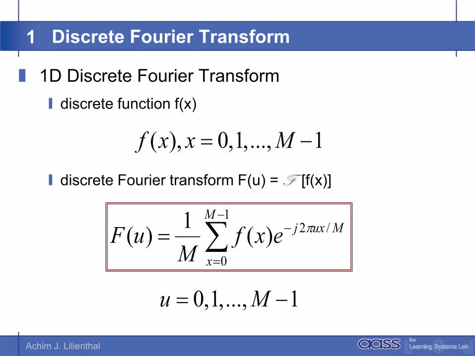
� 1D Discrete Fourier Transform� discrete function f(x)
� discrete Fourier transform F(u) = F [f(x)]
��
�
��1
0
/2)(1)(M
x
MuxjexfM
uF �
1...,,1,0),( �� Mxxf
1...,,1,0 �� Mu
Discrete Fourier Transform1

Achim J. Lilienthal
� 1D Discrete Fourier Transform� discrete function f(x)
� discrete Fourier transform F(u) = F [f(x)]
� think of the Fourier sum (for fixed u) as a dot product between a sinusoid and the original function and remember that dot products measure the projection of one vector in the direction of the other
1...,,1,0),( �� Mxxf
1...,,1,0 �� Mu
Discrete Fourier Transform1
��
�
��1
0
/2)(1)(M
x
MuxjexfM
uF �

Achim J. Lilienthal
Complex Numbers
Euler’s formula)sin()cos( ��� �� je j
22 )))((Im()))((Re()( uFuFuF �
))(sin()())(cos()()( uuFjuuFuF �� �
))(Re( uF ))(Im( uF
]))(Re())(Im([tan)( 1
uFuFu ���
�
with spectrum
phase angle
1

Achim J. Lilienthal
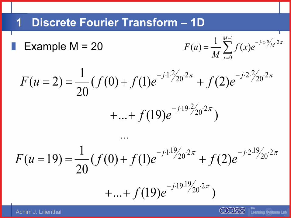
Discrete Fourier Transform – 1D
� Example M = 20 ��
�
��
1
0
2)(1)(M
x
Muxjexf
MuF �
))19(...)1()0((201)0( fffuF ��
))19(...
)2()1()0((201)1(
220119
22012220
11
�
��
�
� �
��
j
jj
ef
efeffuF
1
Achim J. Lilienthal
Discrete Fourier Transform – 1D
� Example M = 20
…
))19(...
)2()1()0((201)2(
220219
22022220
21
�
��
�
� �
��
j
jj
ef
efeffuF
��
�
��
1
0
2)(1)(M
x
Muxjexf
MuF �
))19(...
)2()1()0((201)19(
2201919
220192220
191
�
��
�
� �
��
j
jj
ef
efeffuF
1

Achim J. Lilienthal
Discrete Fourier Transform – 1D
� Notation
)()( uuFuF � �
)()( 0 xxxfxf � �
1

Achim J. Lilienthal
Discrete Fourier Transform – 1D
� Notation
� Units
� for example � [�x] = s � [�u] = s-1 (= Hz) or
� [�x] = m � [�u] = m-1 (= wave number)
)()( uuFuF � �
)()( 0 xxxfxf � �
xMu
���
1
1

Achim J. Lilienthal
Discrete Fourier Transform – 1D
� 1D-DFT Properties� core frequencies (�u/M):
��
�
��
1
0
2)(1)(M
x
Muxjexf
MuF �
u = 0 u = 1 u = 19
…
� F(u=0) � F(u=1) � F(u=19)
1

Achim J. Lilienthal
Discrete Fourier Transform – 1D
� 1D-DFT Properties� core frequencies (�u/M):
� 0
� �u
� …
� (M-1) �u
� F(u) = "frequency component" of f(x)
� each value of F(u) depends on all values of f(x)
��
�
��
1
0
2)(1)(M
x
Muxjexf
MuF �
1
Achim J. Lilienthal
� Standard "Filtering in the Frequency Domain" Procedure� calculate the Fourier Transform F
� process the representation F "in the Fourier domain"
� return to the original domain
Fourier Transform1
Achim J. Lilienthal
Discrete Fourier Transform – 1D
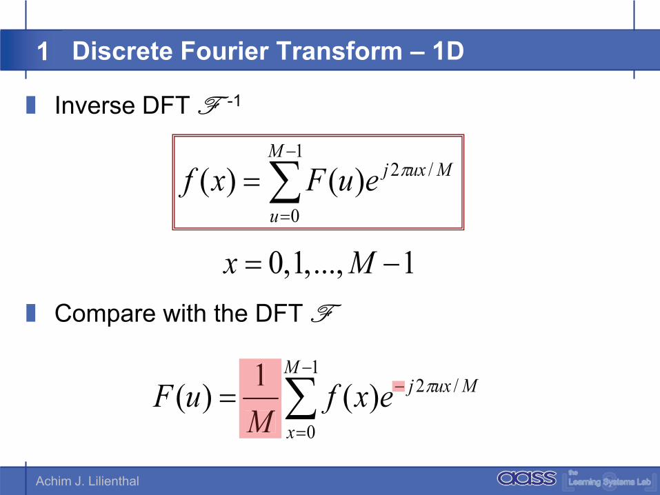
� Inverse DFT FF -1
� Compare with the DFT FF
��
�
�1
0
/2)()(M
u
MuxjeuFxf �
��
�
��1
0
/2)(1)(M
x
MuxjexfM
uF �
1...,,1,0 �� Mx
1M
�
1

Achim J. Lilienthal
Discrete Fourier Transform – 1D1
� Example

Achim J. Lilienthal
Discrete Fourier Transform – 1D
� DFT FF
sampled (0, 1, …, 128-1)
1

Achim J. Lilienthal
Discrete Fourier Transform – 1D
� DFT FF
�
sampled (0, 1, …, 128-1) spectrum = |F(u)|�
1� � 21.20
2127
1282128
12711max �����
���
���
������xM
MuMu

Achim J. Lilienthal
Discrete Fourier Transform – 1D
� DFT FF
�
sampled (0, 1, …, 128-1) spectrum = |F(u)|�
1