Accurate Single Stage Detector Using Recurrent Rolling Convolution

Jimmy Ren Xiaohao Chen Jianbo Liu Wenxiu Sun Jiahao Pang Qiong Yan Yu-Wing Tai Li Xu

SenseTime Group Limited

{rensijie, chenxiaohao, liujianbo, sunwenxiu, pangjiahao, yanqiong, yuwing, xuli}@sensetime.com

Abstract

Most of the recent successful methods in accurate ob-

ject detection and localization used some variants of R-

CNN style two stage Convolutional Neural Networks (CNN)

where plausible regions were proposed in the first stage then

followed by a second stage for decision refinement. Despite

the simplicity of training and the efficiency in deployment,

the single stage detection methods have not been as com-

petitive when evaluated in benchmarks consider mAP for

high IoU thresholds. In this paper, we proposed a novel

single stage end-to-end trainable object detection network

to overcome this limitation. We achieved this by intro-

ducing Recurrent Rolling Convolution (RRC) architecture

over multi-scale feature maps to construct object classifiers

and bounding box regressors which are “deep in context”.

We evaluated our method in the challenging KITTI dataset

which measures methods under IoU threshold of 0.7. We

showed that with RRC, a single reduced VGG-16 based

model already significantly outperformed all the previously

published results. At the time this paper was written our

models ranked the first in KITTI car detection (the hard

level), the first in cyclist detection and the second in pedes-

trian detection. These results were not reached by the pre-

vious single stage methods. The code is publicly available.1

1. Introduction

In many real-world applications, robustly detecting ob-

jects with high localization accuracy, namely to predict the

bounding box location with high Intersection over Union

(IoU) to the groundtruth, is crucial to the quality of ser-

vice. For instance, in vision based robotic arm applications,

the process of generating robust and accurate operations in

picking up an object are highly dependent on the object lo-

calization accuracy. In advanced driver assistance systems

(ADAS), accurately localizing cars and pedestrians is also

1https://github.com/xiaohaoChen/rrc_detection

Figure 1. Left column: Previous single stage detector failed to gen-

erate bounding boxes of high IoU to the groundtruth bounding box

(green) for small and occluded objects; Right column: With the

proposed RRC, we can get high quality bounding boxes.

closely related to the safety of the autonomous actions.

Recent progress in object detection was heavily driven

by the successful application of feed-forward deep Convo-

lutional Neural Networks (CNN). Among many variants of

the CNN based approaches, they can be roughly divded into

two streams. The first is the R-CNN style [9] two stage

methods. In these methods, plausible regions were pro-

posed in the first stage then followed by a second stage for

decision refinement. The other type of methods aimed to

eliminate the region proposal stage and directly train a sin-

gle stage end-to-end detector. The single stage detectors

are usually easier to train and more computationally effi-

cient in production [12]. However, such advantage is largely

overwritten when the models are evaluated in benchmarks

consider mAP for high IoU thresholds (e.g. KITTI car [6])

since the two stage methods are usually advantageous in

performance. We will later show that this weakness of the

single stage methods is not attribute to the inability in rec-

ognizing objects in complex scenes but the failure in gener-

ating high quality bounding boxes. Two examples are illus-

trated in the left column of figure 1.

5420

It can be experimentally shown that most of the low qual-

ity bounding boxes come from the failure localization of

either small objects or overlapping objects. In either case,

conventional bounding box regression becomes highly un-

reliable because the exact locations of the correct bounding

boxes must be determined with the context (e.g. multi-scale

information or feature around the occluded region). That is

why it is effective to resort to some form of context aware

refinement procedure to remove such errors. The RoI pool-

ing and classification stage of Faster R-CNN can be thought

of a simple method to take advantage of such context by re-

sampling feature maps.

In this paper, we show that it is possible to seamlessly

integrate the context aware refinement procedure in a single

stage network. The insight is such procedure can be “deep

in context” by using a novel Recurrent Rolling Convolution

(RRC) architecture. In other words, contextual information

can be gradually and selectively introduced to the bound-

ing box regressor when needed. The whole process is fully

data driven and can be trained end-to-end. We evaluated

our method in the challenging KITTI dataset which consid-

ers mAP for high IoU thresholds. In our experiments, we

used the reduced VGG-16 network instead of the full VGG

network or the more recent ResNet as our pre-trained base

network so that we are able to fully illustrate the effective-

ness of the newly added RRC. This guarantees that such im-

provement is not simply introduced by the more powerful

backbone network. The results showed that our approach

significantly outperformed all the previously published re-

sults by a single model. An ensemble of our models ranks

top among all the methods submitted to the benchmark.

The contributions of our work can be summarized as fol-

lows.

• First, we showed that it is possible to train a single

stage detector in the end-to-end fashion to produce

very accurate detection results for tasks requiring high

localization quality.

• Second, we discovered that the key for improving sin-

gle stage detector is to recurrently introduce context to

the bounding box regression. This procedure can be

efficiently implemented with the proposed Recurrent

Rolling Convolution architecture.

2. Related Work

Convolutional neural network approaches with a region

proposal stage have recently been very successful in the

area of object detection. In the R-CNN paper [9], selec-

tive search [20] was used to generate object proposals, CNN

was used to extract and feed features to the classifier. Two

acceleration approaches to R-CNN were later proposed. In

[8], RoI pooling was used to efficiently generate features

for object proposals. In [16], the authors used CNN instead

of selective search to perform region proposal. Many au-

thors adopted the framework in [16] and proposed a num-

ber of variants which performs well in benchmarks con-

sider mAP for high IoU threshold. For instance, in [23]

the authors proposed to use scale-dependent pooling and

layerwise cascaded rejection classifiers to increase the ac-

curacy and obtained good results. Subcategory information

was used in [21] to enhance the region propose stage and

achieved promising results in KITTI.

One problem with the R-CNN style methods is that in

order to process a large number of proposals the compu-

tation in the second stage is usually heavy. Various single

stage methods which do not rely on region proposals were

proposed to accelerate the detection pipeline. SSD [12] is

a single stage model in which the feature maps with dif-

ferent resolutions in the feed-forward process were directly

used to detect objects with sizes of a specified range. This

clever design saved considerable amount of computation

and performed much faster than [16]. It achieved good re-

sults in datasets for IoU threshold of 0.5. However, we will

show in our experiments that the performance drops signif-

icantly when we increase the bar for bounding box qual-

ity. YOLO [14] is another fast single stage method which

generated promising results, however, it’s not as accurate

as SSD though the customized version is faster. We noticed

that fully convolutional two stage methods [5] has been pro-

posed to reduce the computational complexity of the second

stage. However, it heavily relies on the bigger and deeper

backbone network. The motivation of [7] is similar to ours,

but it does not consider contextual information by using re-

current architecture.

Though Recurrent Neural Networks (RNN) has been

widely adopted in many areas such as image captioning

[11, 22], machine translation [19, 1] and multimedia [15],

the idea of using sequence modelling to improve object de-

tection accuracy has been explored by only a few authors.

An inspiring work is [18] where the authors formalized the

detection problem as a bounding box generation procedure

and used Long Short-Term Memory (LSTM) [10] to learn

this procedure over deep CNN features by using the Hun-

garian loss. It was shown that this method is able to detect

overlapping objects more robustly. However, in this formu-

lation, the first bounding box in the sequence is essentially

determined by a network “shallow in context” because the

first output is only conditioned on the feature extracted by

the last layer of the base network. This may be problem-

atic if the first object in the pipeline is already challenging

(e.g. small object, occluded, out of focus, motion blur, etc.)

to detect which is not uncommon in many real-life applica-

tions. In addition, the method was only evaluated using IoU

threshold of 0.5. Unlike [18], our proposed RRC architec-

ture efficiently detects every object by a network which is

“deep in context” and achieved state-of-the-art performance

5421

under a higher IoU threshold.

3. Analysis and Our Approach

3.1. The Missing Piece of The Current Methods

A robust object detection system must be able to simulta-

neously detect objects with drastically different scales and

aspect ratios. In Faster R-CNN [16], it relies on the large

receptive field of each overlapping 3x3 area of the last con-

volutional layer to detect both small and large objects. Be-

cause multiple pooling layers are used, the resulting reso-

lution of the last layer feature map is much smaller than

the input image. This could be problematic for detecting

small objects because in the low resolution feature map the

features representing the fine details of the small objects is

likely to be weak. Running the network over multi-scale in-

put images as in [17] is one way to mitigate this issue but it

is less computationally efficient.

An insightful alternative was proposed in the SSD paper

[12]. This model exploits the fact that in most of the CNN

models for detection, the internal feature maps in different

layers are already of different scales due to pooling. There-

fore, it is reasonable to utilize the higher resolution feature

maps to detect relatively small objects and the lower res-

olution feature maps to detect relatively big objects. The

advantage of this approach is that it not only provides an

opportunity to localize the small objects more accurately

by relocating the classification and bounding box regression

of these objects to the higher resolution layers, as a single

stage method it is also much faster than the previous two

stage methods because such treatment for multi-scale does

not add extra computation to the original backbone network.

However, SSD is not able to outperform state-of-the-art

two stage methods. Actually, the gap becomes more signif-

icant when high IoU thresholds are used in evaluation. We

now analyze and discuss why this is the limitation of SSD.

We will also show how we addressed such limitation in our

proposed single stage model and achieved state-of-the-art

results in later sections. The utilization of multi-scale fea-

ture maps in SSD can be mathematically defined as follows,

Φn = fn(Φn−1) = fn(fn−1(...f1(I))), (1)

Detection = D(τn(Φn), ..., τn−k(Φn−k)), n>k>0, (2)

where Φn is the feature maps in the layer n, fn(·) is the non-

linear block to transform the feature maps in the (n − 1)thlayer to the nth layer. fn(·) could be the combination

of convolutional layers, pooling layers, ReLU layers, etc.,

f1(I) is the first nonlinear block to transfer the input im-

age I to the first layer feature maps. τn(·) is the function

to transform the nth layer feature maps to the detection re-

sults for a certain scale range. D is the final operation to

aggregate all the intermediate results and generate the final

detection.

According to eq. (2), we can find that it heavily relies on

a strong assumption to perform well. Because the feature

maps in each layer is solely responsible for the output of its

scale, the assumption is that every Φ, by itself, has to be so-

phisticated enough to support the detection and the accurate

localization of the objects of interest. By sophistication it

means that 1) the feature map should have enough resolu-

tion to represent the fine details of the object; 2) the function

to transform the input image to the feature maps should be

deep enough so that the proper high level abstraction of the

object is built-in to the feature maps; 3) the feature maps

contain appropriate contextual information based on which

the exact location of the overlapping objects, occluded ob-

jects, small objects, blur or saturated objects can be inferred

robustly [16, 12, 18]. From eq. (1) and (2), we observed that

Φn is much deeper than Φn−k when k is large, so the afore-

mentioned second condition does not hold for Φn−k. The

consequence is that τn−k(·), the function to transform the

feature maps in the (n − k)th layer to its detection output,

is likely to be a lot weaker and significantly harder to train

than τn(·). Faster R-CNN does not have this depth prob-

lem because its region proposals are generated from the last

layer feature maps, namely

Region proposals = R(τn(Φn)), n > 0. (3)

However, eq. (3) also has its own problem because it does

break the first condition. Therefore, we argue that a more

reasonable function to learn in a single stage detector can

be defined as follows

Detection = D̂(τn(Φ̂n(H)), τn−1(Φ̂n−1(H)),

..., τn−k(Φ̂n−k(H))),

H = {Φn,Φn−1, ...,Φn−k}, n>k>0,

size(Φn−k) = size(Φ̂n−k(H)), ∀k

(4)

where H is a set which contains all the feature maps con-

tribute to the detection function D(·) in eq. (2). Unlike in

eq. (2), Φ̂n(·) is now a function in which all the contribut-

ing feature maps are considered and outputs a new feature

representation of the same dimensionality to Φn.

The function D̂(·) defined in eq. (4) does satisfy the

first two conditions of feature map sophistication because

the feature maps outputted by Φ̂n−k(H) not only share the

same resolution as Φn−k, but also incorporate the features

extracted in the deeper layers. It is worth noting that D̂(·)is still a single stage process though the modification to eq.

(2). In other word, if we can also make eq. (4) satisfy the

third aforementioned condition and devise an efficient ar-

chitecture to train it, we will be able to comprehensively

overcome the limitations of the previous single stage meth-

ods and have the opportunity to surpass the two stage meth-

ods even for high IoU thresholds.

5422

47

159

24

80

12

40

6

203

10

conv4_3 FC6

conv9_2

conv10_2

Conv: 1x1x19Max Pooling

Conv: 1x1x19Max Pooling

Conv: 1x1x19Max Pooling

Conv: 1x1x19Deconv

Conv: 1x1x19Deconv

Conv: 1x1x19Deconv

Conv: 1x1x19Deconv

Conv:2x2x19-p0

conv8_2

19256 19256191925619 1925619 25619

Det

ectio

ns

Conv: 1x1x19Max Pooling

47

159

conv4_3FC6

47

159

24

80

12

40

6

203

10

conv4_3 FC6

conv9_2_2

conv10_2_2

Conv: 1x1x19Max Pooling

Conv: 1x1x19Max Pooling

Conv: 1x1x19Max Pooling

Conv: 1x1x19Deconv

Conv: 1x1x19Deconv

Conv: 1x1x19Deconv

Conv: 1x1x19Deconv

Conv:2x2x19-p0

conv8_2_2

19256 19256191925619 1925619 25619

Det

ectio

ns

Conv: 1x1x19Max Pooling

Conv: 1x1x256 Conv: 1x1x256 Conv: 1x1x256 Conv: 1x1x256 Conv: 1x1x256

159

47conv4_3_2

FC6_2

Figure 2. The Recurrent Rolling Convolution architecture. The diagram illustrates RRC for two consecutive iterations. All the feature maps

(solid boxes) in the first stage including conv4 3, FC6, conv8 2, conv9 2 and conv10 2 were previously computed by the backbone

reduced VGG16 network. In each stage, the arrows illustrates the top-down/bottom-up feature aggregation. All the weights of such feature

aggregation are shared across stages. The selected features by the arrows are concatenated to the neighboring feature maps and illustrated

by the dotted boxes. Between the stages, there are additional 1x1 convolution operators to transform the aggregated feature maps to their

original sizes so that they are ready for the next RRC. These weights are also shared across iterations. Each RRC iteration has its own

outputs and also connects to its own loss functions during training.

3.2. Recurrent Rolling Convolution

RNN for Conditional Feature Aggregation We now de-

fine details in Φ̂(H) so that the feature maps generated by

this function contains useful contextual information for de-

tection. The contextual information in Φ̂(·) means differ-

ently for different objects of interest. For instance, when

detecting small objects it means Φ̂(·) should return fea-

ture maps contain higher resolution features of this object

to represent the missing details. When detecting occluded

objects, Φ̂(·) should return feature maps contain robust ab-

straction of such object so that the feature is relatively in-

variant to occlusion. When detecting overlapping objects,

Φ̂(·) should return feature maps contain both the details of

the boundary and the high level abstraction to distinguish

different objects. Nevertheless, for an intermediate level

feature map such as Φp where p is a positive integer, all

the aforementioned contextual information can be retrieved

either from its lower level counterparts Φp−q or its higher

level counterparts Φp+r, where q and r are also positive

integers. The difficulty is that it is very hard to manually

define a fixed rule for the function Φ̂p(H) to retrieve the ap-

propriate features from Φp−q and Φp+r in H, it is also very

hard to manually select q and r. Therefore, we must system-

atically learn this feature retrieval and aggregation process

from the data.

However, the learning of Φ̂(H) could be troublesome be-

cause H is a set containing multiple feature maps in differ-

ent layers and of different scales and we do not know which

one should be involved and what kind of operations should

be imposed to the feature map for the current object of inter-

est. Therefore, a direct mapping from H to a useful Φ̂(H)have to resort to a considerable size deep network with mul-

tiple layers of nonlinearity. This will not make a computa-

tionally efficient and easy to train single stage network. The

alternative is to design an iterative procedure in which each

step makes a small but meaningful and consistent progress.

This procedure can be mathematically described as follows,

Φ̂t+1p = F(Φ̂t

p, Φ̂tp−1, Φ̂

tp+1;W), t > 0,

Φ̂tn = Φn, ∀n when t = 1,

(5)

where F is a function maps only Φ̂tp and its direct higher

and lower level counterparts at step t to a new Φ̂p at step

t + 1. The function F is parametrized by some trainable

weights W .

The equation is pictorially illustrated in figure 3. We

can see from the figure that I is the input image which is

fed to the network and outputs the feature map Φ̂1. When

the function τ is applied to it for classification and bound-

ing box regression, the output is only conditioned on Φ̂1.

Then the function F shall perform the feature aggregation

5423

Figure 3. Illustration of recurrent feature aggregation.

to bring necessary contextual information and give a new

Φ̂2 at step 2. Then the function τ is able to output a refined

result which is conditioned on the updated feature map Φ̂2.

Note that we can impose a supervision signal to each step

during training so that the system finds useful contextual in-

formation in the feature aggregation to make real progress

in detection. An important insight is that if the weights in Fand τ are shared over steps respectively, this is a recurrent

network. Recurrence can not be overlooked here because it

ensures the consistent feature aggregation across the steps.

This makes the feature aggregation in each step smooth and

generalize well. Otherwise, it will be more prone to overfit-

ting and cause unexpected bias.

RRC Model Details If we simultaneously apply eq. (5)

to every Φ̂, this is our proposed Recurrent Rolling Con-

volution model. It is worth noting that even though Φ̂t+1p

is a function of Φ̂tp and its direct counterparts Φ̂t

p−1 and

Φ̂tp+1, if there are separate F for Φ̂t

p−1 and Φ̂tp+1 respec-

tively for their own direct counterparts, the values in Φ̂t+1p

will eventually be influenced by all the feature maps in Hafter enough iterations.

The proposed RRC model is illustrated in figure 2 in

detail. The figure shows how we applied RRC to the

KITTI dataset using the reduced VGG-16 backbone model

[12, 13]. The size of the input images is 1272x375 with 3

channels, thus the sizes of the original conv4 3 layer and

FC7 layer are 159x47x512 and 80x24x1024 respectively,

where 512 and 1024 are channel numbers. We used addi-

tional 3x3 convolutional layers to further reduce the chan-

nels of them to 256 before feature aggregation. Follow-

ing SSD, we also used the layer conv8 2, conv9 2 and

conv10 2 for multi-scale detection, the difference is that our

conv8 2 layer has 256 instead of 512 channels. We found

the unified channel number among multi-scale feature maps

promotes more consistent feature aggregation.

We used one convolution layer and one deconvolution

layer to aggregate features downwards. For instance, for

the layer conv8 2 a convolution layer with 1x1 kernel is

used to generate feature maps of size 40x12x19. They are

concatenated to FC7 after going through a ReLU and a de-

convolution layer. Likewise, all the left pointing arrows in

the figure indicate such downwards operations. We used

one convolution layer and one max pooling layer to perform

upwards feature aggregation. Also take the layer conv8 2as an example, a 1x1 convolution is followed by ReLU and

max pooling, the resulting 20x6x19 feature maps are con-

catenated to conv9 2. Similarly, all the right pointing ar-

rows in the figure indicate such upwards operations. We call

this feature aggregation procedure “rolling” because the left

pointing and the right pointing arrows resemble it.

Once the rolling is done for the first time, 1x1 convolu-

tion is performed for each layer respectively to reduce the

number of channels to the original setting. After this chan-

nel reduction, the whole feature aggregation is done for the

first iteration. This channel reduction is important because

it ensures a unified shape for every feature map between the

two consecutive feature aggregation. It also makes the re-

current rolling possible. During training, the convolution

kernels corresponding to each arrow as well as the chan-

nel reduction are all shared across iterations. We call this

iterative process recurrent rolling convolution.

RRC Discussion RRC is a recurrent process in which

each iteration gathers and aggregates relevant features for

detection. As we discussed before, these revevant feature

contains contextual information which is critical for detect-

ing challenging objects. For each RRC, there is a separate

loss function to guide the learning of it. This makes sure

that relavant features will be gradually imported and makes

the real progress we expect in every iteration. Because RRC

can be performed multiple times, the resulting feature maps

is therefore “deep in context”. Different from [18], because

RRC is not tailored for any particular bounding box there-

fore the depth in contextual information can be utilized to

detect every object in the scene.

Loss Functions Each iteration has its own loss functions

during training. Following SSD, the loss function for object

category classification was cross-entropy loss. Smooth L1

loss was used for bounding box regression.

Bounding Box Regression Space Discretization In our

setting, a group of feature maps in a layer (e.g. conv4 3) is

responsible for the regression for bounding boxes of a cer-

tain size range. Because the bounding box regression is es-

sentially a linear process, thus if this range is too large or the

feature is too complex, the robustness of the bounding box

regression shall be significantly affected. Because the RRC

process brings more contextual information to the feature

5424

Figure 4. Comparison between SSD and RRC. Left column: re-

sults of SSD, failed to generate bounding box with IoU bigger

than 0.7 to the groundtruth; Middle column: RRC, NMS over out-

put 2 through output 6; Right column: RRC, NMS over output 3

through output 5.

maps, it will inevitably make the feature maps richer based

on which the bounding box regression could be harder to

do for the original object range. To overcome this issue and

make the bounding box regression more robust, we further

discretize the bounding box regression space within a par-

ticular feature maps by assigning multiple regressors for it

so that each regressor is responsible for an easier task.

4. Experiments

The evaluation of our model was performed on the

KITTI benchmark [6] which not only contains many chal-

lenging objects such as small and severely occluded cars

and pedestrians, it also adopts an IoU threshold of 0.7 for

the evaluation in the car benchmark. The KITTI dataset

contains 7481 images for training and validation, and an-

other 7518 images for testing. We did not use any other

dataset in our experiments to enhance the results. The

groundtruth of the test set is not publicly available. One

needs to submit the results to a dedicated server for the per-

formance evaluation of the test set.

We conducted three experiments in this paper. The first

experiment examined the quality of the predictions after

each recurrent rolling convolution. The second one evalu-

ated the performance of our method in a smaller validation

set. The final one evaluated our method in the official test

set and compared with other state-of-the-art methods.

Implementation Details The following settings were

used throughout the experiments. For the network archi-

tecture, we did RRC for 5 times in training. We assigned

5 separate regressors for each corresponding feature map.

Because RRC is performed by 1x1 convolutions, the result-

ing model is efficient. For data augmentation, in addition

to the data augmentation methods adopted in the SSD paper

we also randomly adjusted the exposure and saturation of

the images by a factor of 1.3 in the HSV color space. In

addition, as the minimum scale of the objects in the KITTI

dataset is much smaller than the original configuration, we

adjusted the corresponding scale of conv4 3 from 0.1 to

0.066. We also removed the last global pooling layer of

the original SSD model and set the scale of conv10 2 to

0.85. For learning, stochastic gradient descent (SGD) with

momentum of 0.9 was used for optimization. Weight decay

was set to 0.0005. We set the initial learning rate to 0.0005.

The learning rate will be divided by 10 every 40,000 itera-

tions. We also adopted a simple image similarity metric for

training set and validation set separation. The goal was to

make the training set as different from the validation set as

possible. Our resulting validation set has 2741 images.

4.1. Examining The Outputs After Each RRC

Because RRC was used for 5 times in the training, in

principle our model has 6 outputs, namely the model makes

6 consecutive predictions. According to the design of RRC,

we should be able to observe improvements after each RRC.

The purpose of this experiment is to examine whether this

is indeed the case.

To see the results, we ran a RRC model on both the train-

ing set and the validation set to calculate the average loss for

both sets. The results are summarized in table 1.

The first output is the one before any RRC occurs. The

second prediction happens after the first RRC iteration and

so forth. We can see that the validation loss is generally big-

ger than the training loss. This indicates a certain degree of

overfitting. This is normal because we reserved a significant

portion of the images for the validation set. We observed a

consistent trend in the table. The loss of the second output

is significantly lower than the first one. The lowest loss is

from the third or the fourth output. However, the ensuing

loss values stop to decrease.

Table 1. Average Loss of Different Predictions

Output index Training set Validation set

1 0.662 1.461

2 0.622 1.374

3 0.609 1.357

4 0.607 1.361

5 0.609 1.366

6 0.617 1.375

5425

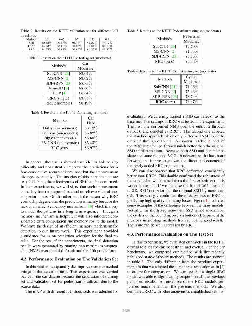
Table 2. Results on the KITTI validation set for different IoU

thresholdsMethods 0.6 0.65 0.7 0.75 0.8

SSD 90.43% 90.15% 89.16% 87.22% 76.12%

RRC* 94.33% 90.78% 90.32% 89.01% 82.19%

RRC 94.52% 90.81% 90.65% 89.27% 82.82%

Table 3. Results on the KITTI Car testing set (moderate)

MethodsCar

Moderate

SubCNN [21] 89.04%MS-CNN [2] 89.02%

SDP+RPN [23] 88.85%Mono3D [3] 88.66%

3DOP [4] 88.64%RRC(single) 89.85%

RRC(ensemble) 90.19%

Table 4. Results on the KITTI Car testing set (hard)

MethodsCar

Hard

DuEye (anonymous) 86.18%Genome (anonymous) 85.82%

eagle (anonymous) 85.66%RV-CNN (anonymous) 85.43%

RRC (ours) 86.97%

In general, the results showed that RRC is able to sig-

nificantly and consistently improve the predictions for a

few consecutive recurrent iterations, but the improvement

diverges eventually. The insights of this phenomenon are

two-fold. First, the effectiveness of RRC can be confirmed.

In later experiments, we will show that such improvement

is the key for our proposed method to achieve state-of-the-

art performance. On the other hand, the reason why RRC

eventually degenerates the prediction is mainly because the

lack of an effective memory mechanism [10] which is a way

to model the patterns in a long term sequence. Though a

memory mechanism is helpful, it will also introduce con-

siderable extra computation and memory cost to the model.

We leave the design of an efficient memory mechanism for

detection to our future work. This experiment provided

a guidance for us on prediction selection for the final re-

sults. For the rest of the experiments, the final detection

results were generated by running non-maximum suppres-

sion (NMS) over the third, fourth and the fifth predictions.

4.2. Performance Evaluation on The Validation Set

In this section, we quantify the improvement our method

brings to the detection task. This experiment was carried

out with the car dataset because the separation of training

set and validation set for pedestrian is difficult due to the

scarce data.

The mAP with different IoU thresholds was adopted for

Table 5. Results on the KITTI Pedestrian testing set (moderate)

MethodsPedestrian

Moderate

SubCNN [21] 73.70%MS-CNN [2] 71.33%

SDP+RPN [23] 70.16%RRC (ours) 75.33%

Table 6. Results on the KITTI Cyclist testing set (moderate)

MethodsCyclist

Moderate

SubCNN [21] 71.06%MS-CNN [2] 75.46%

SDP+RPN [23] 73.74%RRC (ours) 76.47%

evaluation. We carefully trained a SSD car detector as the

baseline. Two settings of RRC was tested in the experiment.

The first one performed NMS over the output 2 through

output 6 and denoted as RRC*. The second one adopted

the standard approach which only performed NMS over the

output 3 through output 5. As shown in table 2, both of

the RRC detectors performed much better than the original

SSD implementation. Because both SSD and our method

share the same reduced VGG-16 network as the backbone

network, the improvement was the direct consequence of

the newly added RRC architecture.

We can also observe that RRC performed consistently

better than RRC*. This double confirmed the robustness of

the conclusion we obtained from the first experiment. It is

worth noting that if we increase the bar of IoU threshold

to 0.8, RRC outperformed the original SSD by more than

6%. This strongly confirmed the effectiveness of RRC in

predicting high quality bounding boxes. Figure 4 illustrated

some examples of the difference between the three models.

Actually, the illustrated issue with SSD is not uncommon,

the quality of the bounding box is a bottleneck to prevent the

previous single stage methods from achieving good results.

The issue can be well addressed by RRC.

4.3. Performance Evaluation on The Test Set

In this experiment, we evaluated our model in the KITTI

official test set for car, pedestrian and cyclist. For the car

benchmark, we compared our method with five recently

published state-of-the-art methods. The results are showed

in table 3. The only difference from the previous experi-

ments is that we adopted the same input resolution as in [2]

to ensure fair comparison. We can see that a single RRC

model was able to significantly outperform all the previous

published results. An ensemble of the RRC models per-

formed much better than the previous methods. We also

compared RRC with other anonymous unpublished submis-

5426

Figure 5. Detection results of our method in KITTI testing set.

sion to KITTI in table 4. By the time this paper was written,

our results for the hardest category ranked the first among

all the submitted methods to the benchmark including all

the unpublished anonymous submissions. To our knowl-

edge, RRC is the first single stage detector to achieve such

result. This result not only confirms the effectiveness of

RRC but also paves a new way for accuracy improvement

for single stage detectors.

RRC also achieved state-of-the-art results on pedestrians

and cyclist benchmark which measures IoU of 0.5. See ta-

ble table 5 and table table 6. Comparing to the previous

published methods, we observed obvious improvements.

When including all the anonymous unpublished submis-

sions, RRC ranks the first for cyclist detection and the sec-

ond for pedestrian detection. This fully justifies the effec-

tiveness and robustness of the proposed RRC model. More

qualitative results are shown in figure 5.

5. Concluding Remarks

In this paper, we proposed a novel recurrent rolling con-

volution architecture to improve single stage detectors. We

found RRC is able to gradually and consistently aggregate

relevant contextual information among the feature maps and

generate very accurate detection results. RRC achieved

state-of-the-art results in all the three benchmarks in KITTI

detection. To our knowledge, this is the first single stage

detector to obtain such convincing results. The code is pub-

licly available.

In the future work, we planned to investigate the mem-

ory enabled recurrent architecture in the context of object

detection and quantify its impact to the detection perfor-

mance. We are also interested in generalizing RRC to the

task of 3D object detection and related applications.

5427

References

[1] D. Bahdanau, K. Cho, and Y. Bengio. Neural machine trans-

lation by jointly learning to align and translate. In ICLR,

2015. 2

[2] Z. Cai, Q. Fan, R. S. Feris, and N. Vasconcelos. A unified

multi-scale deep convolutional neural network for fast object

detection. In ECCV, 2016. 7

[3] X. Chen, K. Kundu, Z. Zhang, H. Ma, S. Fidler, and R. Urta-

sun. Monocular 3d object detection for autonomous driving.

In CVPR, 2016. 7

[4] X. Chen, K. Kundu, Y. Zhu, A. Berneshawi, H. Ma, S. Fidler,

and R. Urtasun. 3d object proposals for accurate object class

detection. In NIPS, 2015. 7

[5] J. Dai, Y. Li, K. He, and J. Sun. R-fcn: Object detection via

region-based fully convolutional networks. In NIPS, 2016. 2

[6] A. Geiger, P. Lenz, and R. Urtasun. Are we ready for au-

tonomous driving? the kitti vision benchmark suite. In

CVPR, 2012. 1, 6

[7] S. Gidaris and N. Komodakis. Locnet: Improving localiza-

tion accuracy for object detection. In CVPR, 2016. 2

[8] R. Girshick. Fast r-cnn. In ICCV, 2015. 2

[9] R. Girshick, J. Donahue, T. Darrell, and J. Malik. Rich fea-

ture hierarchies for accurate object detection and semantic

segmentation. In CVPR, 2014. 1, 2

[10] S. Hochreiter and J. Schmidhuber. Long short-term memory.

Neural Computation, 9(8):1735–1780, 1997. 2, 7

[11] A. Karpathy and F.-F. Li. Deep visual-semantic alignments

for generating image descriptions. In CVPR, 2015. 2

[12] W. Liu, D. Anguelov, D. Erhan, C. Szegedy, S. Reed, C.-Y.

Fu, and A. C. Berg. SSD: Single shot multibox detector. In

ECCV, 2016. 1, 2, 3, 5

[13] W. Liu, A. Rabinovich, and A. C. Berg. Parsenet: Looking

wider to see better. In arxiv. 1506.04579, 2015. 5

[14] J. Redmon, S. Divvala, R. Girshick, and A. Farhadi. You

only look once: Unified, real-time object detection. In

CVPR, 2016. 2

[15] J. Ren, Y. Hu, Y.-W. Tai, C. Wang, L. Xu, W. Sun, and

Q. Yan. Look, listen and learn - a multimodal lstm for

speaker identification. In AAAI, 2016. 2

[16] S. Ren, K. He, R. Girshick, and J. Sun. Faster r-cnn: To-

wards real-time object detection with region proposal net-

works. TPAMI, 38(1):142–158, 2016. 2, 3

[17] P. Sermanet, D. Eigen, X. Zhang, M. Mathieu, R. Fergus,

and Y. LeCun. Overfeat: Integrated recognition, localization

and detection using convolutional networks. In ICLR, 2014.

3

[18] R. Stewart, M. Andriluka, and A. Y. Ng. End-to-end people

detection in crowded scenes. In CVPR, 2016. 2, 3, 5

[19] I. Sutskever, O. Vinyals, and Q. Le. Sequence to sequence

learning with neural networks. In NIPS, 2014. 2

[20] J. R. R. Uijlings, K. E. A. van de Sande, T. Gevers, and

A. W. M. Smeulders. Selective search for object recognition.

IJCV, 104(2):154–171, 2013. 2

[21] Y. Xiang, W. Choi, Y. Lin, and S. Savarese. Subcategory-

aware convolutional neural networks for object proposals

and detection. In ECCV, 2016. 2, 7

[22] K. Xu, J. Ba, R. Kiros, K. Cho, A. Courville, R. Salakhutdi-

nov, R. Zemel, and Y. Bengio. Show, attend and tell: Neural

image caption generation with visual attention. In ICML,

2015. 2

[23] F. Yang, W. Choi, and Y. Lin. Exploit all the layers: Fast and

accurate cnn object detector with scale dependent pooling

and cascaded rejection classifiers. In CVPR, 2016. 2, 7

5428