accurate camera calibration and feature based 3-d ... · accurate camera calibration and feature...
TRANSCRIPT

Accurate camera calibration and featurebased 3-D reconstruction from monocular
image sequences
by
Janne Heikkilä


Heikkilä, Janne: Accurate camera calibration and feature based 3-D reconstructionfrom monocular image sequencesInfotech Oulu and Department of Electrical Engineering, University of Oulu, FIN-90570Oulu, FinlandActa Univ. Oul. C 108, 1997Oulu, Finland(Received 10 October, 1997)
Abstract
In this thesis, computational methods are developed for measuring three-dimensional structure fromimage sequences. The measurement process contains several stages, in which the intensityinformation obtained from a moving video camera is transformed into three-dimensional spatialcoordinates. The proposed approach utilizes either line or circular features, which are automaticallyobserved from each camera position. The two-dimensional data gathered from a sequence of digitalimages is then integrated into a three-dimensional model. This process is divided into three majorcomputational issues: data acquisition, geometric camera calibration, and 3-D structure estimation.
The purpose of data acquisition is to accurately locate the features from individual images. Thistask is performed by first determining the intensity boundary of each feature with subpixel precision,and then fitting a geometric model of the expected feature type into the boundary curve. The resultingparameters fully describe the two-dimensional location of the feature with respect to the imagecoordinate system. The feature coordinates obtained can be used as input data both in cameracalibration and 3-D structure estimation.
Geometric camera calibration is required for correcting the spatial errors in the images. Due tovarious error sources video cameras do not typically produce a perfect perspective projection. Thefeature coordinates determined are therefore systematically distorted. In order to correct thedistortion, both a comprehensive camera model and a procedure for computing the model parametersare required. The calibration procedure proposed in this thesis utilizes circular features in thecomputation of the camera parameters. A new method for correcting the image coordinates is alsopresented.
Estimation of the 3-D scene structure from image sequences requires the camera position andorientation to be known for each image. Thus, camera motion estimation is closely related to the 3-D structure estimation, and generally, these two tasks must be performed in parallel causing theestimation problem to be nonlinear. However, if the motion is purely translational, or the rotationcomponent is known in advance, the motion estimation process can be separated from 3-D structureestimation. As a consequence, linear techniques for accurately computing both camera motion and 3-D coordinates of the features can be used.
A major advantage of using an image sequence based measurement technique is that thecorrespondence problem of traditional stereo vision is mainly avoided. The image sequence can becaptured with short inter-frame steps causing the disparity between successive images to be so smallthat the correspondences can be easily determined with a simple tracking technique. Furthermore, ifthe motion is translational, the shapes of the features are only slightly deformed during the sequence.
Keywords: subpixel accuracy, image distortion, motion estimation, 3-D measurement


Acknowledgements
This study was carried out in the Machine Vision and Media Processing Group at theDepartment of Electrical Engineering of the University of Oulu, Finland and the TechnicalUniversity of Denmark, Copenhagen during the years 1993-1997.
I would like to express my gratitude to Professor Matti Pietikäinen for allowing me towork in his laboratory and providing me with excellent facilities for completing this thesis.I am also grateful to my supervisor Professor Olli Silvén for his guidance and support. Itwas very kind from him to release me from the routine paper work and give me enough timeto carry out the research. Without his enthusiastic and encouraging attitude this thesiswould not have ever seen the light of day. Furthermore, I would like to thank ProfessorBjarne Ersboell from the Technical University of Denmark for the collaboration during myresearch visit.
I am grateful to Dr. Visa Koivunen for fruitful discussions and advice on estimationproblems. I also appreciate his comments on this work. Professor Henrik Haggrén and Dr.Ilkka Moring are acknowledged for reviewing the thesis. Their critical but pertinentcomments clearly improved the quality of the manuscript.
I wish to thank my colleagues in the laboratory including Lasse Jyrkinen, HannuKauniskangas, Hannu Kauppinen, Jukka Kontinen, Timo Ojala, Hannu Rautio, TapioRepo, Jukka Riekki, Dr. Juha Röning and Dr. Jaakko Sauvola for creating a pleasantatmosphere.
This work was financially supported by the Graduate School in Electronics,Telecommunications and Automation, Technology Development Centre of Finland, TaunoTönning Foundation, and Nordic Research Network in Computer Vision. Their support isgratefully acknowledged.
I am deeply grateful to my mother Margit and father Alpo for their love and care overthe years. My sister Pirkko and brothers Esko, Kari and Jukka deserve also warm thanksfor their unconditional support. Most of all, I want to thank my dear wife Anne for herpatience and understanding.
Oulu, September 4, 1997 Janne Heikkilä


List of symbols and abbreviations
Mathematical notations
H+ pseudoinverse of HHT transpose of H
estimate of p(p)N normalization of px average of xE[x] expectation of x
Latin letters
a1,..., a8 inverse distortion model coefficientsDu, Dv conversion factors from metric units to pixelseu, ev root mean square error in image coordinatesf focal lengthh height of the image sensorI(u, v) image intensity value in (u, v)k1, k2 radial distortion coefficientsM number of images in the sequenceN number of points or featurespi = [xi, yi, zi]
T location vector of the point Pip1, p2 tangential distortion coefficientsQ(u, v) algebraic distancesu image scale factor in the horizontal directiontk = [tx, k, ty, k, tz, k]
T translation vector at time instant ku, v horizontal and vertical image coordinatesu0, v0 coordinates of the principal point
principal point centered image coordinatesprincipal point centered distorted image coordinates
p
u v,u'˜ v'˜,

δu(r), δv(r) radial distortion componentsδu(t), δv(t) tangential distortion componentsU, V measured image coordinates
coordinates of the focus of expansion at time instant kx, y, z, X, Y, Z Cartesian coordinates
Greek letters
αk motion scale factor at time instant kθk = [ ]T 2-D location vector of the FOE at time instant kσ standard deviation of the measurement noiseω, ϕ, κ Euler angles
Abbreviations
2-D two-dimensional3-D three-dimensionalCCD charge-coupled deviceCCIR monochrome video format specified by International
Radio Consultive Committee (Comite ConsultatifInternational des Radiocommunications)
CoG center of gravityCRLB Cramer-Rao lower boundDLT direct linear transformationEKF extended Kalman filterFOE focus of expansionFOV field of viewIEKF iterated extended Kalman filterIRLS iterative reweighted least squaresLS least squaresPLL phase locked loopRAC radial alignment constraintRMS root mean squareRMSE root mean square errorRS-170 Electronic Industries Association (EIA) standard for
monochrome videoSMPT sample-moment-preserving transformSVD singular value decompositionTLS total least squares
Uk V k,
Uk V k,

Contents
AbstractAcknowledgementsList of symbols and abbreviationsContents1. Introduction ......................................................................................................... 11
1.1. Background...............................................................................................111.2. The scope of the thesis..............................................................................131.3. The contributions of the thesis..................................................................151.4. The outline of the thesis............................................................................16
2. Data acquisition for accurate 3-D computer vision............................................. 182.1. Introduction...............................................................................................182.2. Image labeling...........................................................................................20
2.2.1. Template matching ........................................................................202.2.2. Hough transform............................................................................22
2.3. Refining data.............................................................................................232.3.1. Coarse precision edge detection ....................................................232.3.2. Fitting in the image domain...........................................................252.3.3. Moment based fitting.....................................................................262.3.4. Moment preserving ellipse detection.............................................28
2.4. Extracting feature parameters ...................................................................312.4.1. Line fitting .....................................................................................322.4.2. Direct quadratic curve fitting.........................................................332.4.3. Minimizing the geometric distance ...............................................362.4.4. Approximations of the geometric distance....................................372.4.5. Renormalization ............................................................................382.4.6. Direct intensity based parameter estimation..................................392.4.7. Robust parameter estimation .........................................................40
2.5. Discussion.................................................................................................423. Geometric camera calibration ............................................................................. 44
3.1. Introduction...............................................................................................443.2. Camera model ...........................................................................................45

3.3. Calibration methods..................................................................................483.3.1. Nonlinear minimization.................................................................483.3.2. Self-calibration ..............................................................................493.3.3. Direct linear transformation ..........................................................503.3.4. Multi-step methods........................................................................523.3.5. Implicit methods............................................................................553.3.6. Other methods ...............................................................................56
3.4. Inverse model and image correction .........................................................573.5. Measurement error sources .......................................................................59
3.5.1. Hardware .......................................................................................603.5.2. Calibration target ...........................................................................613.5.3. Projection asymmetry with circles ................................................613.5.4. Illumination ...................................................................................643.5.5. Focus and iris.................................................................................67
3.6. A calibration procedure for circular control points ..................................683.7. Discussion.................................................................................................69
4. Motion estimation and 3-D reconstruction ......................................................... 704.1. Introduction...............................................................................................704.2. 3-D shape from a single view ...................................................................714.3. Kalman filtering........................................................................................72
4.3.1. Motion estimation..........................................................................724.3.2. Structure estimation.......................................................................75
4.4. Batch technique.........................................................................................764.5. Linear motion estimation ..........................................................................76
4.5.1. Epipolar constraint.........................................................................774.5.2. Motion from the focus of expansion .............................................804.5.3. Accuracy of the motion estimate ...................................................844.5.4. Scale factor ....................................................................................874.5.5. Elimination of rotations .................................................................88
4.6. Linear reconstruction ................................................................................904.6.1. CRLB for reconstruction accuracy................................................914.6.2. Accuracy of the measurement system ...........................................92
4.7. Visual tracking..........................................................................................954.8. Discussion.................................................................................................97
5. Experiments......................................................................................................... 995.1. Hardware and test setup............................................................................995.2. Subpixel edge detection and feature extraction ......................................1005.3. Camera calibration..................................................................................1025.4. Motion estimation ...................................................................................1055.5. Structure estimation ................................................................................108
6. Conclusions ....................................................................................................... 113References .................................................................................................................. 115Appendix AAppendix B

1. Introduction
1.1. Background
Extracting three-dimensional information from two-dimensional image coordinates is anessential problem in computer vision. Applications of this measurement technique can befound, for example in the areas of autonomous vehicle guidance, surveying, industrialmanufacturing, quality control and video surveillance. The nature of the application setsthe requirements for the measurement process. In robot navigation, the real-time perform-ance is often more important than the measurement accuracy. On the other hand, manufac-turing or assembling sophisticated mechanical parts may require high precision 3-Dmeasurements even at the cost of the production speed.
The 3-D information extracted is typically either a range map or a set of 3-D coordi-nates. In addition, it may also contain the estimated position and orientation of the sensor.The 3-D information is calculated based on the disparities between multiple views, or, insome cases, known constraints of a monocular view. There are basically two different ap-proaches: a feature based approach and an optical flow technique. Due to accuracy andspeed requirements, it is often preferable to direct the image processing resources intosmall regions of interest with high information contents than to operate with the whole im-age. Only a relatively small number of carefully selected relevant features should be ex-tracted, depending on the situation and on the requirements of the task; knowledge shouldbe applied to maximize the efficiency in processing the selected features (Dickmanns &Graefe 1988). The optical flow approach is based on the relationship between the changein intensity at a given pixel location between frames and the spatial intensity gradient of asmall neighborhood of that pixel (Horn & Schunck 1981). However, the optical flow tech-nique typically suffers from high computational intensity.
The features can be natural or artificial. The natural features are, for example, edges,corners, curves, or surface patches characteristic of the objects in view, whereas the artifi-cial features are, for example, special markers or light stripes produces by a laser beam.The measurement technique is passive, if recognition of the features is based on the ambi-ent lighting present in the scene, and active, if the features are produced by an external lightsource. Passive optical techniques may be grouped into triangulation based methods, in-

12
cluding traditional theodolite measurements, image based photogrammetry and stereo vi-sion, and other methods providing shape information from monocular images (Moring1995). Active 3-D imaging is typically based on a triangulation principle, where a light pat-tern is projected onto the scene, and by using the known geometry between the sensor andlight source, the 3-D structure of the target object can be reconstructed. Other active meth-ods are, for example, imaging radars, Moiré technique, and holographic interferometry(Besl 1988). The image sequence based approach is active or passive depending on themethod of producing the features.
The features are either 3-D or 2-D depending on the sensor used in measurements. Basedon the feature types Huang and Netravali (1994) defined the following three categories ofproblems and applications:
• 3-D to 3-D feature correspondences. Applications are: a) motion estimation usingstereo or other range finding devices, and b) positioning a known 3-D object usingstereo or other range finding devices.
• 2-D to 3-D feature correspondences. Applications are: a) single camera calibration,i.e., determination of position and orientation of a camera knowing some features of3-D objects as imaged on the camera, and b) passive navigation of a vehicle using asingle camera and based on the knowledge of 3-D landmarks.
• 2-D to 2-D feature correspondences. Applications are: a) finding relative attitudes oftwo cameras which are both observing the same 3-D features, b) estimating motionand structure of objects moving relative to a camera, c) passive navigation, i.e., find-ing the relative attitude of a vehicle at two different time instants, and d) efficient cod-ing and noise reduction of image sequences by estimating motion of objects.
The approaches for solving these problems are disparate. This thesis concentrates on thesecond and the third problems with the following applications: monocular camera calibra-tion and estimating motion and structure from image sequences.
Intensity images captured using a video camera and a frame grabber can be consideredas 2-D signals which are contaminated by measurement noise composed of systematic andrandom parts. In accurate 3-D reconstruction of the scene structure, the problem of estimat-ing the original 2-D signal becomes evident. A good camera calibration technique is there-fore needed to compensate for the systematic noise component. The random part of themeasurement noise causes uncertainty in the observed image coordinates of the features.The main source of the random variation is signal quantization. There are also other minornoise types that originate from the detector, CCD array, and electronics. The effect of therandom measurement noise cannot be fully removed, but by using appropriate estimationtechniques the effect can be minimized.
Not only the quality of the observations, but the 3-D estimation technique selected hasa great influence on the accuracy of the results. Two types of methods have been used for3-D motion and structure analysis (Weng et al. 1993). The first type is iteratively solvingnonlinear equations, and the second type is solving the problem using linear algorithms.The iterative methods are typically computationally intensive and the linear methods arehighly sensitive to noise. The estimation techniques presented in the literature are often

13
based on the extended Kalman filter (Faugeras et al. 1992, Dickmanns & Graefe 1988,Matthies et al. 1988), batch least squares (Spetsakis & Aloimonos 1992, Weng et al. 1993),or epipolar geometry (Thompson 1959, Longuet-Higgins 1981, Tsai & Huang 1984).
In camera calibration, as well as in motion and structure estimation, both iterative andlinear techniques have been developed. The iterative methods (Slama 1980, Weng et al.1992) utilize nonlinear camera models. They are rather slow if compared with linear tech-niques, but their accuracy has been shown to be much greater. On the other hand, lineartechniques (Abdel-Aziz & Karara 1971, Faugeras & Toscani 1986, Melen 1994) producea closed-form solution which is not very accurate, but it can be used as a starting point foran iterative search. In addition, a very famous calibration method was suggested by Tsai(1987), where a subset of the camera parameters were estimated using a linear techniqueand the rest of the parameters were derived iteratively.
Techniques for performing accurate camera calibration and recovering 3-D informationfrom 2-D images has been widely studied and applied in the field of photogrammetry forapproximately one hundred years. Much of the time, the focus has been on the productionof topographic mapping from aerial imagery. During the past few decades, the invention ofthe digital imagery has broadened the spectrum of the applications from traditional areas toindustrial and engineering measurements. Today, a typical photogrammetric station con-sists of several solid state video cameras that are steadily mounted around the measurementvolume. The proportional accuracy achieved with this kind of technique is often better than1/10000 (Haggrén 1992).
The science of photogrammetry, with its emphasis on exploitation of digital imagery,has common links with the field of computer vision. What separates the two fields, howev-er, is the focus of photogrammetry on matters related to accuracy aspects. In computer vi-sion, the emphasis has been more in development of human like vision systems. However,in order to fully utilize the digital image data in 3-D measurements, it is necessary to com-bine the knowledge from both of these fields.
1.2. The scope of the thesis
The purpose of this thesis is to develop techniques for producing accurate 3-D informationfrom 2-D image sequences. The accuracy requirements are not specified here explicitly,since the performance of the techniques depends on the measurement arrangements and theconfiguration of the features. Therefore, the results obtained are compared with theoreticallimits existing for those circumstances. The 3-D information, as it is considered here, in-cludes a set of coordinate triplets (xi, yi, zi), i = 1, 2,... that specifies the geometric formof one or several target objects. These triplets are expressed either in a local object centeredcoordinate system or in a global coordinate system, which can be also used to determinethe relationship between different objects or sensors. The 3-D information is produced fromcorresponding 2-D image coordinates (ui, vi). For each feature point, there can be severalobservations obtained from different camera positions and orientations.
The amount of data in an image sequence is tremendous. A typical sequence can havemore than a hundred images, and each image consists of several hundreds of thousands ofpixels. Most of the data is insignificant, and therefore, some image processing and estima-

14
tion stages are applied in order to get rid of the irrelevant parts of the data, and to filter theremaining information in such a way that an optimal 3-D interpretation of the image obser-vations is obtained. The solutions given in this thesis are mainly based on estimation theo-ry. We shall adopt the following viewpoint towards that theory: estimation theory is theextension of classical signal processing to the design of digital filters that process uncertaindata in an optimal manner (Mendel 1995).
The task of producing the 3-D information can be subdivided into three independentproblems: data acquisition, calibration, and 3-D reconstruction. In data acquisition, all thenecessary parameters of the features are extracted from 2-D images. The number and themeaning of these parameters or attributes depend on the feature geometry. In this thesis,only line and circular primitives are considered, because they are the most common shapesin man-made objects, and they can be fully characterized by only a few parameters. For linefeature, two parameters need to be solved, whereas five parameters are needed in order todescribe the elliptic projection of a circle completely. There are several different phases inthe process of determining the feature parameters. Subpixel boundary detection and modelbased fitting are examined more closely due to their importance in minimizing the meas-urement noise. The feature geometry is assumed to be known in advance.
The sensor calibration problem is evident for all measurement devices. In image se-quence based 3-D measurement, the sensor is a video camera which is a complex opto-elec-tric device, and obtaining a complete model of its operation is practically impossible. Onlyapproximate models can therefore be used. A geometric camera model typically performsthe mapping from 3-D world coordinates to 2-D image coordinates. The model contains aset of unknown parameters that are solved in camera calibration based on image observa-tions of either a known or unknown control point structure. The procedure described in thisthesis requires prior knowledge about the mutual 3-D locations of the control points. Theparameters are solved from an overdetermined set of equations by minimizing the sum ofsquared residuals. Circular control points are examined as a special case, because they re-quire an additional calibration step. The inverse mapping from 2-D image coordinates to 3-D lines-of-sight is then determined, based on the camera parameters obtained. There arealso several error sources that are not considered in the camera model, but still they can af-fect the accuracy of the calibration procedure and the 3-D reconstruction. Some of theseerror sources are also examined in this thesis.
Producing a 3-D model from 2-D coordinates of an image sequence is the third problemconsidered in this thesis. There are three tasks attached to the problem: camera motion es-timation, structure estimation, and resolving the feature correspondences. The first and thesecond tasks are closely related. The structure cannot be determined from an image se-quence without knowing the camera poses with respect to a fixed coordinate frame. How-ever, in the presence of noise, disregarding information that is related to the structure of thescene results in less reliable estimates of motion parameters since this information is alsorelated to motion (Weng et al. 1993). Thus, solving camera motion and thereby the cameraposes in general requires information about 3-D structure of the scene. As a consequence,both motion and structure must be determined at the same time. However, by reducing thespace of free motion parameters the procedures can be separated. The motion estimationmethod introduced in this thesis makes use of only translational components of the motionparameters, assuming that camera rotation is eliminated. The 3-D coordinates of the fea-tures are then solved, based on the motion estimate, and the known correspondences be-

15
tween the frames. The third task, resolving the feature correspondences is slightlyproblematic in a multi-camera stereo system. The scene may have quite a diverse appear-ance from different viewpoints causing great difficulty in automatic processing of corre-spondences. However, in the image sequence based approach the apparent motion of thefeatures between the successive frames is relative short if the images are captured frequent-ly. The correspondence problem can be now solved by using an automatic feature trackingtechnique.
The methods proposed in this thesis have been tested with both simulated and real imagedata using Matlab® software1. The accuracy of the methods is verified by comparing theresults with the Cramer-Rao lower bound that gives the smallest error covariance attainableunder certain conditions. Matters related to the implementational aspects of the measure-ment system are also briefly considered.
1.3. The contributions of the thesis
In this thesis, several techniques have been developed for obtaining accurate 3-D data fromimage sequences. The idea of determining motion and structure from feature correspond-ences is not new. Good descriptions of the existing methods are given by Huang andNetravali (1994) and Weng et al. (1993). However, less attention has been paid to accuracy.The main contribution of this thesis is the development of an accurate image sequencebased 3-D measurement technique. There are several novelties comprised in the differentparts of the 3-D measurement process:
• A moment based edge detection method for elliptic features. Especially in cameracalibration, it is necessary to determine the control points to the highest possibleaccuracy. The moment based edge detector introduced in this thesis locates the circu-lar and elliptic feature boundaries with subpixel precision. A geometric model is thenfitted to the boundary curve in order to estimate the unknown parameters of the fea-ture.
• An inverse camera model. Camera calibration typically produces mapping from 3-Dcoordinates to 2-D image coordinates. However, in most 3-D applications mappingfrom image coordinates to line-of-sight directions is needed. This problem can besolved by using a novel inverse camera model whose parameters are derived from thephysical camera parameters.
• Asymmetry correction for circular features. Circles are projected as ellipses in theimage plane. Perspective projection causes the centroids of the ellipses to be slightlydisplaced from the actual projection of the circle centers. The calibration procedureproposed in this thesis compensates for the asymmetry error, and enables a moreaccurate solution for the camera parameters.
1 Matlab is a registered trademark of The MathWorks Inc.

16
• Error source analysis in camera calibration. There are several disturbances in theimage formation process that are not considered in a typical camera model. Espe-cially the camera optics are afflicted by various physical phenomena that can degradethe measurement accuracy when the overall imaging conditions have changed.
• A linear method for camera motion estimation. Generally, camera motion estimationrequires knowledge about the scene structure. However, in most cases this informa-tion is not available. A linear epipolar constraint based method (Thompson 1959,Longuet-Higgins 1981, Tsai & Huang 1984) can be used, but it has been reported toprovide relative low accuracy in the presence of noise. A new focus of expansionbased technique is introduced in this thesis which provides accurate information onrotation free camera motion without knowing the 3-D structure of the scene inadvance.
• Accuracy analysis is performed for the camera translation based measurement tech-nique. A proportional accuracy of 1/10000 is consider to be a realistic objective forthe suggested technique.
The techniques developed in this thesis enable a reasonably inexpensive and fast solutionfor automatic 3-D measurement. Only a single video camera, a frame grabber and a lineartrack with a simple conveyer mechanism is required. In the absence of natural features, thefeature pattern may be produced by a separate laser projector equipped with a special latticethat spreads the ray into several beams. The numerical computation is performed by ameasurement software running in a standard PC system. An illustration of the systemframework is shown in Fig. 1.
1.4. The outline of the thesis
The remaining chapters of the thesis are organized as follows:
Chapter 2 concentrates on data acquisition, i.e., locating the feature from 2-D images. Itbriefly discusses about segmenting the images into features and background. After segmen-tation, several subpixel edge detection methods are represented, and a new moment basedtechnique is also suggested. The rest of the chapter deals with the feature extraction prob-lem. Some direct and iterative least squares techniques are reviewed for fitting the geomet-ric model of the feature projection to the edge data observed. A brief overview to the robustmethods is also given.
Chapter 3 describes the geometric camera calibration problem, and it represents some ofthe most important calibration approaches. A new method is proposed for image correctionand backprojection. At the end of the chapter, calibration errors due to external disturbanc-es are discussed.

17
Chapter 4 deals with the 3-D reconstruction problem. It represents the extended Kalmanfilter based solution, and the batch estimation technique. It then breaks the problem intoseparate motion and structure estimation tasks. The epipolar constraint is considered as ageneral solution, but, due to its poor accuracy, a translational motion based approach is de-veloped. An accuracy analysis is performed for the measurement technique, and as a resulta simple equation for approximate proportional accuracy is derived. At the end of the chap-ter, visual tracking techniques are also briefly discussed.
Chapter 5 presents the experiments made in different phases of the measurement process.The performances of the feature extraction and calibration methods are validated with realimage data. For 3-D reconstruction, simulations have also been used because of the lack ofaccurate reference objects.
Chapter 6 concludes the thesis and presents ideas for future work.
Appendix A presents the algorithm for determining the ellipse boundary in subpixel reso-lution by using the moment based approach.
Appendix B gives the algorithm for performing the renormalization conic fitting for theellipse edge data.
Object
Projected
Stepper motor
Motion
.. ..... ...... .....points
Light
DataAcquisition
CameraCalibration
3-DReconstruction
projector
Image
3-DModel
Fig. 1. Illustration of a single camera based measurement system.
.. . ... .. ... . ... .. ... . ... .. ... . ... .. .Calibrationtarget

2. Data acquisition for accurate 3-D computervision
2.1. Introduction
Data acquisition in 3-D computer vision is a process of extracting spatial information from2-D images. In a feature based approach, this information consists of geometrical proper-ties that are characteristic to each feature type. For line features, the data may include twoparameters: the distance and orientation, but for ellipses, a set of five parameters is neces-sary to describe their geometry entirely. In order to extract this information, several opera-tions must be performed. Haralick and Shapiro (1992) suggested the following six steps:image formation, conditioning, labeling, grouping, extracting, and matching. These stepsconstitute a canonical decomposition of the data acquisition problem, each step preparingand transforming the data in the right way for the next step. The amount of data transmittedis reduced during the process, but the information contents that we are interested in are notlost. This sequence of steps and the data transmitted is depicted in Fig. 2a.
The first step, image formation, is not addressed in this thesis. We assume that there isan intensity image available that represents the scene of visible features. The second step,conditioning, is based on a model which suggests that the observed image is composed ofan informative pattern modified by uninterested variations that typically add to or multiplythe observed image or change the geometric relations in the image. These variations are ei-ther systematic error or random noise. Some systematic error components originating in theimage formation process are discussed in the context of camera calibration in Chapter 3. Incase of random noise, the purpose of conditioning is to suppress it. However, from thestandpoint of accurate 3-D reconstruction, noise filtering often decreases the informationcontents of the image, and, therefore, should not be applied.
The third step, labeling, is based on a model which suggests that the informative patternhas structure as a spatial arrangement of events, each spatial event being a set of connectedpixels. Labeling determines what kind of spatial events each pixel participates in. For ex-ample, if the interesting spatial events of the informative pattern are events only of high-valued and low-valued pixels, then the thresholding operation can be considered a labelingoperation. Other kinds of labeling operations include edge detection, corner finding, and

19
identification of pixels that participate in various shape primitives. (Haralick & Shapiro1992.)
In grouping step, the labeled pixels are connected to larger regions based on their spatialrelations. For example, if the labels are symbolic, the grouping is actually a connected com-ponents operation. There are several standard techniques for performing this operation. Formore information the reader is referred to Haralick & Shapiro (1992).
The extracting step is also called feature extraction, for example by Nadler and Smith(1993). The objective of this step is to compute a list of properties or parameters for eachgroup of pixels. Example properties might be centroid, area, and orientation. Parameter es-timation is carried out by fitting a geometric model to the data obtained from the previousstep. The model fitted is expected to correspond to the shape of the feature. It can be, forexample, line, circle, ellipse, or parabola. The feature type is often assumed to be known inadvance.
The matching operation determines the interpretation of some related set of imageevents, associating these events with some given 3-D object or 3-D shape (Haralick &Shapiro 1992). In image sequence based 3-D measurement application, the matching prob-lem becomes the detection of the feature correspondences between the successive frames.This task is discussed in more detail in Chapter 4.
1. Image formation
5. Extracting
6. Matching
Fig. 2. The sequence of steps needed for data acquisition (a) generally in computer visionaccording to Haralick and Shapiro (1992), and (b) in accurate 3-D computer vision.
2. Conditioning
3. Labeling
4. Grouping
1. Image formation
5. Refining
6. Extracting
2. Conditioning
3. Labeling
4. Grouping
7. Matching(a)
(b)
intensity image
preprocessed image
spatial events
regions of interest
edge data
feature parameters
set of parameters
3-D structure estimationor camera calibration

20
When spatially accurate data acquisition is required, it is not practical to strictly followthe schema suggested by Haralick and Shapiro. It is proposed in this thesis that a new step,refining, is added between steps 4 and 5 (see Fig. 2b). The purpose of this step is to rectifythe positional accuracy of the features detected. This is performed by first locating the fea-ture boundary with coarse precision, and then determining it more accurately with somesubpixel edge detection technique.
In this chapter, we will concentrate on the labeling, refining, and extracting steps. Linesand ellipses are used as features due to their simple mathematical formulation and theircommonness in man-made scenes. Some robust methods for handling the outliers in datasets are also described. The data acquisition techniques proposed here can be utilized bothin the camera calibration and 3-D reconstruction discussed in the following chapters.
2.2. Image labeling
Various labeling operations can be found from the literature. The principles of these oper-ations depend on the spatial events they are designed to detect, and they typically requiresome prior knowledge about the feature type. In this section, we restrict ourselves to iden-tifying the pixels that participate either in lines or ellipses, and the type of the features aregiven in advance. For this purpose, the principles of template matching and Hough trans-form are briefly presented.
2.2.1. Template matching
Template matching is probably the most common method for determining various primi-tives from 2-D images. It is based on the principle that the features can be detected by com-paring the image data with a prototype. This comparison can be performed by using cross-correlation. Peaks in the output image show the locations of the possible matches. Howev-er, the requirement of a prototype restricts the usage of this approach. For example, in thecase of line features, the orientation should be known in advance, or several prototypes indifferent orientations should be applied. In the case of circular features, the orientation isnot a problem, but the size of the circle should be approximately known.
Another matching technique that was applied, for example by Heikkilä and Silvén(1995) is the morphological hit-and-miss transformation (Serra 1982). It is an operation toselect pixels that have certain geometric properties. The hit-and-miss transformation can beused for various purposes, but, for template matching, it was first applied by Crimmins andBrown (1985). Unlike the correlation method, the hit-and-miss transformation gives us apossibility to loosen the exact-matching idea to tolerance matching. This is a useful prop-erty, because the dimensions of the prototype rarely correspond exactly to the features inthe image. The following definition of the transformation is obtained from Haralick &Shapiro (1992).
Let J and K be two structuring elements that satisfy . The hit-and-missJ K∩ ∅=

21
transformation of set A by structuring elements J and K is denoted by A ⊗ (J, K) and is de-fined by
(2.1)
where is the binary erosion operation and Ac is the binary complement of A.If we want an exact match of a template T in a binary image I, we can use transformation
I ⊗ (T, W − T), where W is a window within which the template T is situated, i.e., .The exact matching idea is loosened by using K-tolerance matching
(2.2)
where K is a small disklike structuring element and ⊕ is the binary dilation operation.As we can notice, the hit-and-miss transformation is a binary technique, and therefore,
the image must be first thresholded. As a consequence, a lot of information is lost duringthis operation, causing the result to become inaccurate. However, the hit-and-miss transfor-mation can be used for approximately locating the feature points in the image and to usethat information for focusing the attention to smaller regions. An example of the hit-and-miss transformation is shown in Fig. 3. In the original image, there is a white object withseveral dark circular feature points on its surface. There are also some other objects in thebackground that make the data acquisition process more complicated. Applying the hit-and-miss transformation produces a binary image in which we can notice that almost allfeature points have been detected. After the connected component analysis (grouping), wehave a reasonably good guess about the locations of the features in the image.
A ⊗ J K,( ) A o- J( ) Ac o- K( )∩=
o-
W T⊇
H I ⊗ T o- K W T K⊕( )–,( )=
Fig. 3. The hit-and-miss transformation: (a) the original image, and (b) the result of thetransformation.
(a) (b)

22
2.2.2. Hough transform
The Hough transform (Hough 1962, Illingworth & Kittler 1988) is a method for detectingstraight lines and curves from grey level images (Haralick & Shapiro 1992). It is based onparametrization of the particular geometrical forms it is designed to detect. For instance, acommon line equation d = u cos α + v sin α consists of image coordinates (u, v) and param-eters (α, d). For each image coordinate pair (u, v), there exists an infinite number of param-eters (α, d) that can satisfy the equation. The basic idea in the Hough transform is toquantize the parameter space (α, d) to a set of discrete values αj and dj. Then, for eachline observation (ui, vi) there is only a finite number of matches in the parameter space thatcan satisfy the discretized equation dj = ui cos αj + vi sin αj. These matches are added to a2-D accumulator array whose entries represent the quantized values of the parameter space.A peak in the accumulator array reveals those parameter values that are most likely to rep-resent the line in the image.
Using the Hough transform for detecting more complex features is straightforward. Thedimension of the accumulator array must correspond to the number of unknown parame-ters. For example, detecting ellipses requires a five-dimensional array. The algorithm iswell-known, and therefore it is not considered here. For more information, the reader is re-ferred to Haralick & Shapiro (1992) and Illingworth & Kittler (1988). The Hough trans-form can be also generalized to detect arbitrary shapes for any orientation and scale. It isthen called the generalized Hough transform (Ballard 1981).
Using the Hough transform requires quantization of the parameters. This quantization isusually coarser than the natural quantization of the image plane. As a result, the accuracyof the parameter estimate can be rather poor. On the other hand, increasing the sample ratedecreases the robustness of detection. If quantization is dense, the peaks in the accumulatorarray are not sharp, and they may be spread over neighboring cells due to the measurementnoise. In addition, the size of the array grows rapidly as the number of the samples is in-creased. For example, doubling the sample rate requires eight times more cells in the caseof a three-dimensional parameter space. As a consequence, the Hough transform as it wassuggested by Hough (1962) is quite rarely applied to solve problems having more thanthree unknowns.
Detecting conics would require a five-dimensional parameter space that is computation-ally too costly. In order to solve this problem, many algorithms and modified methods havebeen proposed. For example, Illingworth and Kittler (1987) used a multiple resolution ap-proach to reduce the amount of computation, Yip et al. (1992) suggested an approach fordetecting circles and ellipses, where the use of parallel edge points reduces the parameterspace to two dimensions. Some hybrid techniques also exist that use the Hough transformas a part of the detection process, for example the fast ellipse and circle detector proposedby Ho and Chen (1995) that is based on the principle of the geometric symmetry of the fea-tures to be detected.
The Hough transform is used here as a labeling technique, but it can be also consideredas an extracting method, because it produces the estimates of the feature parameters. How-ever, the accuracy of the parameters obtained is not adequate for 3-D measurement purpos-es. Thus, the greatest advantage of the Hough transform is that it can be used to detectvarious geometric shapes from complex scenes, and to focus the attention of the subsequentimage processing steps.

23
2.3. Refining data
The purpose of the refining step is to determine the contrast boundaries, i.e. the edges ofthe features with subpixel precision. If we consider the human vision system, there are threetypes of object boundaries that can be perceived (Nadler & Smith 1993):1. Contrast boundaries, that is, loci of points where the gray-scale changes fairly
abruptly.2. Textural boundaries, that is, loci of points where two “textures” abut.3. Optical illusion boundaries created by a completion property of human vision. These
boundaries are sometimes called “gestalt boundaries”.The first case is the most common way to discriminate an object from the background incomputer vision, and it is also the simplest, because only the gray-scale discontinuities needto be detected. The other two types require more sophisticated statistical or structural meth-ods, and therefore, they are not considered here.
There are various methods for detecting gray-scale edges, but using convolution masksis probably the most popular approach. Implementation is then straightforward enablingfast real-time image processing. However, the major disadvantage is that the resolution islow. More sophisticated edge detection techniques must be applied for obtaining higher ac-curacy. These subpixel techniques are often based on some edge model which is fitted tothe gray-level data around the edge profile. There are different edge approximations, butalso different fitting criteria like least-squares minimization and moment preserving. Ap-proaches other than model based fitting exist, for example, statistical edge detection pro-posed by Åström and Heyden (1996), and a method proposed by Tabbone and Ziou (1992)that corrects the edge location by using the edge model and first or second order filter prop-erties. However, most of the subpixel precision edge detection methods are suitable foronly straight edges. Only few techniques are available for detecting curved features like el-lipses.
2.3.1. Coarse precision edge detection
Gradient operators are based on the presumption that the intensity profile is abruptlychanged across the edge. The gradient magnitude G = then has a peakin the location where the edge is steepest. One of the early gradient based edge operatorswas employed by Roberts (1965). He used the following two 2 by 2 masks to calculate thegradient across the edge in diagonal directions:
The masks are translated pixel by pixel over the image and in each position a weighted sumof four neighboring pixels is computed. Letting r1 be the value calculated using the firstmask and r2 the value calculated using the second mask, the gradient magnitude will be
.As an example of 3 by 3 gradient based neighborhood operators, the Prewitt operator
dI du⁄( )2 dI dv⁄( )2+
R11 0
0 1–= R2
0 1–
1 0=
r12 r2
2+

24
(Prewitt 1970) consists of the following two orthogonal masks:
Letting the output of these masks be p1 and p2 respectively, the gradient magnitude will be and the direction tan-1(p1/p2).
The square root and trigonometrical computation is avoided by using compass masks forquantized set of directions. For example, Kirsch (1971) proposed the following set ofmasks:
The gradient magnitude for the Kirsch masks is max kn, n = 0,...,7 and the gradient direction45˚argmax kn.
Another mathematical model that has been suggested for edge detection is the secondorder derivative of the intensity profile, also called the Laplacian operator
(2.3)
The place where the gradient has its maximum is the same place as the second derivativehas a zero-crossing. On the both sides of the edge the response is non-zero. These regionsare called dark or light edges, depending on the sign of the response. Like the gradient op-erator, the Laplacian is also a linear operator. As a result, it can be calculated by finite-dif-ference convolutions over digital images. For example, the Laplacian masks for 3 by 3 and5 by 5 neighborhoods are (Nadler & Smith 1993)
It can be noticed that for linearly varying intensity surfaces, the response is always zero.This makes the Laplacian operator a high-pass filter. In order to avoid the high frequencynoise peaks being amplified, the image should be prefiltered before edge detection.
In practice, all convolution mask operators are applied at every pixel of the entire imageor smaller window, and the points of local maxima (minima) or the points above (below) a
P1
1– 0 1
1– 0 1
1– 0 1
= P2
1 1 1
0 0 0
1– 1– 1–
=
p12 p2
2+
K0
3– 3– 5
3– 0 5
3– 3– 5
= K1
3– 5 5
3– 0 5
3– 3– 3–
= K2
5 5 5
3– 0 3–
3– 3– 3–
= K3
5 5 3–
5 0 3–
3– 3– 3–
=
K4
5 3– 3–
5 0 3–
5 3– 3–
= K5
3– 3– 3–
5 0 3–
5 5 3–
= K6
3– 3– 3–
3– 0 3–
5 5 5
= K7
3– 3– 3–
3– 0 5
3– 5 5
=
LI
2u v,( )∂u2∂
--------------------- I2
u v,( )∂v2∂
---------------------+=
L3
1– 1– 1–
1– 8 1–
1– 1– 1–
= L5
0 1– 1– 1– 0
1– 1 0 1 1–
1– 0 8 0 1–
1– 1 0 1 1–
0 1– 1– 1– 0
=

25
given threshold value are selected. This limits the resolution of the detected edge locationto one pixel. However, the coarse information obtained by using convolution masks can beused as initial guess for more accurate methods.
2.3.2. Fitting in the image domain
It was shown by Haralick and Shapiro (1992) that a least squares fit of a linear surface mod-el over 2 by 2 neighborhood produces exactly times the Roberts gradient discussedin the previous section. The linear model produces the gradient magnitude for each neigh-borhood, but it does not give any information about the gradient peaks where the edge isactually located. The gradient peaks can be determined from the zero crossings of the sec-ond order derivatives. For a linear model, the second order derivative is always zero. Thus,a more comprehensive surface model is needed.
Haralick (1984) assumed that the intensity profile in any image neighborhood can bemodelled with a third order polynomial (facet model). He used this model to locate the edgefrom the zero crossing of the second directional derivative taken in the direction of the gra-dient. To compute the coefficients of the model, a set of orthogonal filters based on discreteChebyshev polynomials is applied to a two-dimensional image neighborhood. This ap-proach works well for blurred edges where the gradient is rather smooth. For sharp edgesthe cubic approximation can introduce large deviations.
Nalwa and Binford (1986) showed that the zero-crossing can result in extremely bad lo-calization when a step-edge is located near the boundary of the image window. They alsoclaimed that zero-crossing operators do not adequately exploit the local intensity profile ofstep edges. To correct the problem, they proposed a 1-D tanh (hyperbolic tangent) fit alongthe gradient direction. This approach gives a good fit for step edges, but it requires a non-linear search that can be rather exhaustive due to the highly nonlinear nature of the tanh-function.
It was already noted in the previous section that Laplacian filters amplify the high fre-quency noise, and therefore, the image should be first prefiltered. This was also the basicidea in the subpixel edge detector proposed by Huertas and Medioni (1986). They con-volved the image with Laplacian-of-Gaussian (LoG) masks and applied a second order fac-et model to the filtered image. Using this model, they first increased the resolution of theimage by interpolation and then detected the zero-crossings with subpixel precision. It wasshown by Verbeek and van Vliet (1994) that the Laplacian operator produces a bias in edgelocation that is away from the center of the curvature, while the second derivative in thegradient direction (SDGD) produces a shift that is in the opposite direction. They, there-fore, proposed an edge detector called PLUS that is a sum of the Laplacian operator andSDGD. In both of these approaches, the image is prefiltered in order to reduce the high fre-quency noise. However, this filtering also smooths the details and decreases the edge de-tection precision.
Kisworo et al. (1994) emphasized that there are also other types of edges than step edg-es, such as roofs, ramps, etc. As a result, they presented a subpixel edge detection techniquethat utilizes a general edge model. Their technique was able to detect and classify the edgeinto some predefined categories. To perform this, a specific edge model is fitted to the local
1 2⁄

26
energy of the image region in a least squares sense. The model is selected based on the re-sponse of local energy filters. Kisworo et al. claimed that this technique does not sufferfrom the problem of amplification of high-frequency noise, and it does not detect false pos-itives arising from points of inflection, or points of maximum gradient.
2.3.3. Moment based fitting
The most common edge type in man-made objects is a step edge, and therefore we are alsomost interested in locating them with subpixel precision. However, fitting a step edge to theintensity data by minimizing the squared error in the image domain may produce unsatis-factory results due to its highly non-linear nature. This problem is illustrated in Fig. 4,where a 1-D step edge is fitted to the set of spatially quantized observations. The sum ofthe squared errors ε2 as a function of the edge position x is plotted below. The error attainsits minimum in xd where it has a constant value. The width of xd is one pixel which impliesthat subpixel resolution cannot be achieved without interpolation.
In order to detect step edges Hueckel (1971) used the fitting idea with low-frequencypolar-form Fourier basis functions on a circular disk. The fitting was done by expandingboth the ideal step edge and the image region being examined in terms of a set of orthogonalbasis functions and minimizing the sum of the squared differences between correspondingcoefficients. To simplify the computation, the expansion was truncated to nine terms. Somemodification of this approach can be found from the literature, for example O’Gorman(1978) used Walsh functions instead of Fourier basis functions in a square window, andHummel (1979) applied a set of optimal basis functions derived from the Karhunen-Loèveexpansion of the local image values.
A slightly different approach for fitting the step edge to the image data was introducedby Tabatabai and Mitchell (1984). Instead of minimizing the squared error, they fitted apredefined model to the measured intensity data I(u, v) with the first three sample momentsbeing preserved. The edge detector uses as the input data a set of 69 pixels, chosen so thatthe detection area will best approximate a circle with a radius r of 4.5 pixels. The weight-ings wj, j = 1,..., 69 associated with those pixels depend on their area inside the circle. Thus,
Fig. 4. Least squares fitting of a 1-D step edge to the observed intensity values.
x
x
I(x)
true edge
observedintensity values
ε2(x)
xd

27
the pixels in the perimeter that are partly outside are less weighted than the pixels complete-ly inside the circle. This is illustrated in Fig. 5a.
The edge model proposed by Tabatabai and Mitchell (1984) is a step edge that dividesthe detection circle into two adjacent regions A1 and A2 with areas a1 and a2 respectively(see Fig. 5b). The edge between the regions is assumed to be nearly straight locally. Forboth regions there are constant intensities H1 and H2 with their relative frequency of occur-rence P1 and P2, where P1 + P2 = 1. The image areas a1 and a2 are proportional to P1 andP2, i.e., a1 = P1πr2 and a2 =P2πr2. The following relations can be now written for the firstthree sample moments Mi:
(2.4)
A direct solution for parameters H1, H2, P1 and P2 is obtained based on Eq. (2.4). The di-rection of the edge normal α can be estimated from the image gradient. The distance l isderived based on the geometry of Fig. 5b.
Before using this type of detector, the edge location must be approximately known tosuch accuracy that the error is less than the radius of the detection area. This step is per-formed, for example, by applying one of the convolution masks discussed in Section 2.3.1.to the region of interest found in the labeling and grouping stages. The circular detectionarea is then centered over the detected edge pixels and their position is finally correctedbased on the estimated parameters α and l.
Tsai (1985) used this technique for image thresholding and he called it the sample-mo-ment-preserving transform (SMPT). Later, the same principle has been utilized in severalapplications, e.g., accurate line detection (Chen & Tsai 1988a), corner detection (Liu &Tsai 1990), pattern matching (Chou & Chen 1990), and clustering (Liu & Tsai 1989). Aslightly different approach formed the basis of the edge detector suggested by Lyvers et al.
w1 w2 w3 w4 w5
w12 w11 w10 w9 w8 w7 w6
w14w15 w16 w17w18 w19 w20w13 w21
w29w28 w27 w26 w24 w24 w23w30 w22
w32w33 w34 w35 w36 w37 w38w31 w39
w47w46 w45 w44 w43 w42 w41w48 w40
w50w51 w52 w53 w54 w55 w56w49 w57
w64w63 w62 w61 w60 w59 w58
w65 w66 w67 w68 w69
Region A1
Region A2
α
(a2, H2, P2)
(a1, H1, P1)
x
y
(a) (b)
Linear edgeapproximation
l
Fig. 5. (a) Circular edge detection area, and (b) the moment based linear edge model.
P 1H 1i 1 P– 1( )H 2
i+ M i w jIi u j v j,( ) i
j 1=
69
∑ 1 2 3, ,= = =

28
(1989). Instead of using the gray-scale moments, they preserved the first three spatial mo-ments in a circular image region. Otherwise, the approach was quite similar to the SMPT.
2.3.4. Moment preserving ellipse detection
For curved features, like ellipses, the linear edge approximation will produce inexact esti-mates of the edge location. For obtaining greater accuracy, a different edge model shouldbe used. However, a direct solution to the problem becomes very difficult with the momentpreserving technique, and there are only few suggestions to solve this problem in the liter-ature.
Lee et al. (1990) presented a direct method for estimating ellipse parameters based onthe moment preserving principle. The ellipse position was detected with a center of gravitymethod, which is not a very accurate method in case of noisy images. In addition, only bi-level (binary) images were used. Very similar analysis based on the second order ellipsemoments was also given by Haralick and Shapiro (1992).
Safaee-Rad et al. (1991) used Tabatabai and Mitchell’s (1984) principle for detectingcurve pixels. Their idea was to detect the intersection of the linear edge approximation anda circular arc that was used to model the curved edge segment. These intersection points(x3, y3) and (x4, y4) are depicted in Fig. 6a. It was claimed that the radius R of the circulararc has only a small effect on the relative position of these points along the edge line, andtherefore, a correction term can be generated based on its mean value. The correction termsfor different line distances l are recorded in a look-up-table (LUT). The intersection pointsare then recovered from the line equation obtained using Tabatabai and Mitchell’s edge de-tector. However, Safaee-Rad et al. (1991) did not consider the error in the line normal di-rection α. It is quite obvious that even a small deviation in this angle can cause a large errorin the location of the intersections (x3, y3) and (x4, y4). It would be preferable to estimatethe intersection of the line normal and the circular arc, but then there should be some wayof estimating the radius R.
Chen and Tsai (1988b) proposed a moment-preserving curve detection method in whichthey used parabolic equations to estimate the curve shape within the detection circle. Theellipse parameters were estimated based on first and second order spatial moments from aset of nonlinear equations. An iterative numeric technique was applied to solve these equa-tions because no direct methods exist. The problem is that the computational intensity fordetecting a single ellipse becomes high, since several edge points, sometimes even morethan hundred, may be needed.
The approach presented here is based on the assumption that the local curvature of theellipse is know in advance. This is feasible, because the edge pixels are located with lowprecision already before applying the subpixel detector, which only refines the edge loca-tion for those pixels. Coarse estimates for ellipse parameters can be calculated using theedge pixel locations. A reasonably accurate estimate for curvature is then obtained analyt-ically for each edge pixel. The remaining problem is nonlinearity. Using a circular detec-tion area results always in a set of nonlinear equations for the edge parameters. Thisproblem can be avoided by introducing a square n by n detection window illustrated in Fig.6b, where coefficients wi are set to be equal. For example, in the case of n = 7 each cell in

29
the window is weighted by 1/49.Let us consider the composed area Ai = Ri + Si + Ti shown in Fig. 7a. By using the same
gray level moment preserving principle as Tabatabai and Mitchell (1984), we can solve thecomposed area from Eq. (2.4). On the other hand, if we decide to approximate the edge seg-ment inside the square with a second order curve , we can write the fol-lowing expression for the composed area Ai:
(2.5)
where gi = [gu, i, gv, i]T is the normal vector of the local edge profile so that ||gi|| = 1. This
vector can be estimated based on the spatial moments inside the detection window. A sim-ilar solution for determining the edge direction was also proposed by Tabatabai andMitchell (1984).
The parameter ai is obtained from the local curvature κi, so that ai = κi / 2. In the caseof Fig. 7a, the parabola is limited to the opposite margins of the detectionwindow. Thus, the expression for x0, i becomes
(2.6)
The width di of the rectangle Ti can be solved from Eq. (2.5) when we know the composedarea Ai. Finally, the correction for the edge pixel (Ui, Vi) is calculated based on the knowngeometry of Fig. 7a.
Region A1
Region A2
α
(a2, H2, P2)
(a1, H1, P1)
(x1, y1)
(x2, y2)
(x3, y3)
(x4, y4)
x
y(x0, y0)
R
G
Fig. 6. (a) Edge model suggested by Safaee-Rad et al., and (b) a square edge detection area forelliptic features.
(a)
Linear edgeapproximation
l
w1 w2 w3 w4 w5 w6 w7
w8 w9 w10 w11w12 w13 w14
w15 w16 w17 w18 w19 w20 w21
w22 w23 w24 w25 w26 w27 w28
w29 w30 w31 w32 w33 w34 w35
w36 w37 w38 w39 w40 w41 w42
w43 w44 w45 w46 w47 w48 w49
(b)
y ai x2 x0 i,2–( )=
Ai43---aix0 i,
3 2 gu i, gv i, x0 i,2 ndi+ +=
y ai x2 x0 i,2–( )=
x0 i,n 2 gv i,( )⁄ gu i, gv i,≤,n 2 gu i,( )⁄ otherwise,
=

30
In the other configuration, shown in Fig. 7b width di is zero and the area Ai consists oftwo segments Ri and Si, i.e., Ai = Ri + Si. Again, the estimate for the area Ai is obtained basedon the moment preserving principle, but the parameter x0, i must be determined from thefollowing equation:
(2.7)
There are three possible roots of the equation, but only one real solution exists:
(2.8)
where
(2.9)
and
(2.10)
The refined position of the edge pixel (Ui, Vi) is calculated based on the known geometryof Fig. 7b. A more comprehensive description of this algorithm is given in Appendix A.
Implementation of the procedure is straightforward, and the computational cost is lowerthan in the method proposed by Chen and Tsai (1988a) because no iterations are required.The performance of this method is compared with the method proposed by Safaee-Rad etal. (1991). The results are presented in Chapter 5.
ig. 7. Edge model for elliptic features with two spatial configurations.
Ri
Si
x
y
y = ai(x2 - x0,
2i)
Ti
x0, i
-x0, i
di
(a)
Ri
Si
x
y
y = ai(x2 - x0,
2i)
x0, i
-x0, i
.(0,-aix0,2
i)
.(0,aix0,2
i)
(b)
.(Ui,Vi) .(Ui,Vi)
gi
gi
Ai43---aix0 i,
3 2 gu i, gv i, x0 i,2+=
x0 i,ai
2ti2 3⁄
ρiaiti1 3⁄ ρi
2+–
4ai2ti
1 3⁄---------------------------------------------------=
ti
24Aiai2 ρi
3– 4ai 3Ai 12Aiai2 ρi
3–( )+
ai3
------------------------------------------------------------------------------------------=
ρi 2 gu i, gv i,=

31
2.4. Extracting feature parameters
After edge detection, the feature parameters are extracted. This operation is performed byfitting a geometric model of the expected feature projection to the edge data. Depending onthe feature shape, a certain number of parameters are estimated. There are several parame-ter estimation techniques that can be applied, for example, least squares (LS), maximumlikelihood (ML), mean squared (MS), and maximum a posteriori (MAP) estimation. Typi-cally, estimation of the model parameters requires solving a set of nonlinear equations.However, in some cases a direct method is also available.
Least squares (LS) fitting is probably the most common method for solving estimationproblems. It uses the principle that the sum squared error between the observations and themodel is minimized. There may be various error criteria, but typically only one is optimalin the sense of finding the minimum variance unbiased estimate (MVUE). The error termminimized depends on the noise characteristics. Here, we first restrict ourselves to imageobservations, where both coordinates are contaminated by independent and identically dis-tributed additive Gaussian noise, and then broadened to distributions where a few samplesdeviate greatly from others.
In order to minimize the error term a certain distance measure must be used to weightindividual observations. Three distance measures are considered here: algebraic, geomet-ric, and statistical distance. The algebraic distance leads to a direct linear solution that is,with only few exceptions, not as accurate as can be achieved by minimizing the geometricdistance. On the other hand, the geometric distance does not completely agree with the sta-tistical distance in the case of nonlinear models.
Let us define the general equation of a conic to be
(2.11)
This equation represents all quadratic curves (circles, ellipses, parabolas, and hyperbolas)and also lines when A = B = C = 0. If we denote N observed edge points by , where
, the algebraic distance between the observation and the curve is Q(Ui, Vi).The function to be minimized becomes
(2.12)
The other two distance measures are examined later.We may notice that there is a trivial solution for the minimization problem of Eq. (2.12):
A = B = C = D = E = F = 0. In order to avoid this, Q(u, v) should be normalized. There areseveral normalization methods for both line and quadratic curve fitting proposed in the lit-erature. Two normalizations for line fitting (E = -1, D2 + E2 = 1), and three normalizationsfor quadratic curve fitting (F = 1, A + C = 1, A2 + B2 + C2 + D2 + E2 + F2 = 1) are consideredhere. In the case of line fitting, the nonlinear parts of Eq. (2.11) are omitted and only thelast three parameters (D, E, F) are estimated.
Q u v,( ) Au2 Buv Cv2 Du Ev F+ + + + + 0= =
Ui V i,( )i 1 … N, ,=
J1 Q Ui V i,( )2
i 1=
N
∑=
32
2.4.1. Line fitting
Using the normalization E = -1, Eq. (2.11) is reduced to a form of v = Du + F that is prob-ably the most commonly used line presentation in the literature. Let us denote p1 = [D, F]T,ai = [Ui, 1]T, H = [a1, a2,..., aN]T, and v = [V1, V2,..., VN]T. Now, the dependence betweenthe observations and the line parameters can be expressed by using the linear model
(2.13)
where η is a N by 1 noise vector. Our objective is to determine the parameter estimatethat minimizes the sum of the squared terms of vector η. The LS solution is found by usingthe pseudoinverse technique
(2.14)
The notation H+ symbolizes the Moore-Penrose inverse (or pseudoinverse) of the matrix H(Strang 1988). However, there are a couple of problems that restrict the usage of this ap-proach. The first problem is that the linear model in Eq. (2.13) has a singularity when theline is vertically oriented. This may cause the estimator to fail in certain constellations ofthe observed edge points. The other problem is that the least squares estimator of Eq. (2.14)assumes that the explaining variables in the matrix H are noise free, and only the verticalcomponent of the measurement error is minimized. The actual noise characteristics do nottypically fulfil this condition.
Haralick and Shapiro (1992) employed the principle of minimizing the sum of thesquared residuals under the constraint that D2 + E2 = 1. Using the Lagrange multiplier form,the error function can be expressed as
(2.15)
The function J2 is minimized by forcing its partial derivatives with respect to D, E, and Fto zero. After some algebra, the following estimate of the parameter vector p2 = [D, E]T
is obtained:
(2.16)
where is the sample variance in u-direction and is the sample covariance. The term is the smallest eigenvalue of the sample covariance matrix
(2.17)
By denoting bi = [Ui, Vi]T the estimate of parameter F becomes
(2.18)
v Hp1 η+=
p1
p1 H+v=
J2 DUi EV i F+ +( )2 λ D2 E2 1–+( )N–i 1=
N
∑=
p2
p21
S uv2 S u
2 λ–( )2
+----------------------------------------
S uv–
S u2 λ–
=
S u2 S uv
λ
SS u
2 S uv
S uv S v2
=
F1N---- bi
T p2
i 1=
N
∑–=

33
It can be shown that the estimate in Eq. (2.16) is the eigenvector corresponding to the small-est eigenvalue. Thus, the estimate is also obtained by using the eigenvalue-eigenvectorfactorization of the matrix
(2.19)
where ΛS is a 2 by 2 diagonal matrix containing the eigenvalues λS1 and λS2, and QS is a2 by 2 orthonormal matrix containing the eigenvectors qS1 and qS2 in its columns. The es-timate becomes
(2.20)
Let us consider the following expression for the orthogonal geometric distance di be-tween the line Du + Ev + F = 0 and the point i located in position (Ui, Vi):
(2.21)
We notice that minimizing the error function J2 under the constraint D2 + E2 = 1 is equiv-alent to minimizing the sum of the squared orthogonal distances between the line and ob-servations. Due to this property, the estimate is also called the total least squares (TLS)estimate (Golub & Van Loan 1989). Using the TLS technique for motion estimation is dis-cussed in Chapter 4.
The performance of the estimators in Eqs (2.14) and (2.20) is illustrated in Fig. 8 withtwo examples. The observations in Fig. 8a are from a vertical line causing the pseudoin-verse based estimator (solid line) to fail because of singularity, while the TLS based esti-mator (dashed line) works correctly. In Fig. 8b there is one measurement point deviatingstrongly from the pattern. The estimator of Eq. (2.14) minimizes the squared error alongthe vertical axis causing the outlier point to have a much larger impact on the result thanother observations. The estimator of Eq. (2.20) minimizes the sum of squared distances inan orthogonal direction that is less influential to outliers than the vertical direction.
2.4.2. Direct quadratic curve fitting
There are many different possible normalizations for quadratic curve fitting. However, thefollowing three normalizations are very often used in the literature (e.g. Rosin 1993, Zhang1995, Porrill 1990). Let us first consider the normalization with F = 1. If we denote
, L = [d1, d2,..., dN]T, r = [1, 1,...,1]T, and the parameter vec-tor p3 = [A, B, C, D, E]T, the problem becomes to solve the linear equation
(2.22)
where η is a N by 1 noise vector. The solution can be found by applying the pseudoinversetechnique
p2
S QSΛSQST=
p2
p2 qSi where i min λSj( )arg= =j 1 2,=
di
DUi EV i F+ +
D2 E2+----------------------------------------=
p2
di Ui2 UiV i V i
2 Ui V i, , ,,[ ]T
=
r L– p3 η+=

34
(2.23)
Normalizing the conic equation with F = 1 implies that the position of the origin pointshould be selected in such a manner that the curve does not go through it. Otherwise, sin-gularity is encountered.
A slightly different estimator is obtained by applying the normalization A + C = 1. Letus denote , M = [e1, e2,..., eN]T, s = [ , ,..., ]T, andthe parameter vector p4 = [A, B, D, E, F]T. Again, the estimator is obtained by using thepseudoinverse technique
(2.24)Unlike in the case of F = 1 the normalization A + C = 1 is translation and rotation invariantfor elliptical features.
The third normalization considered here is A2 + B2 + C2 + D2 + E2 + F2 = 1. The ap-proach is basically the same as when normalizing the line equation with D2 + E2 = 1. Usingthe notation , and N = [f1, f2,..., fN]T, the estimate of theparameter vector p5 = [A, B, C, D, E, F]T can be obtained from the eigenvalue-eigenvectorfactorization of the square matrix R = NTN:
(2.25)
where ΛN is a 6 by 6 diagonal matrix containing the eigenvalues λN1,..., λN6, and QN is a6 by 6 orthogonal matrix containing the eigenvectors qN1,..., qN6 in its columns. The esti-mate becomes
(2.26)
Fig. 8. Line fitting with normalization E = -1 (solid line) and D2 + E2 = 1 (dashed line): (a)in the case of a vertical line, and (b) in the case of one outlier in observations.
(a) (b)
p3 L– +r=
ei Ui2 V i
2– UiV i Ui V i 1, , ,,[ ]T
= V 12 V 2
2 V N2
p4 M– +s=
f i Ui2 UiV i V i
2 U, i V i 1, , ,,[ ]T
= p5
R QNΛNQNT=
p5
p5 qNi where i min λNj( )arg= =j 1 … 6, ,=

35
This solution minimizes the orthogonal distances between the vectors fi and their projec-tions on data subspace spanned by eigenvectors corresponding to the five largest eigenval-ues. The estimate is a TLS solution to the quadratic curve fitting problem. However, thedistance minimized here is not the same as the orthogonal geometric distance between theobservations and the curve, and, unlike in line fitting, this estimate is not optimal in thesense of minimizing the geometric distance.
Rosin (1993) compared the first two normalizations in the case of ellipse fitting andfound out that setting F = 1 is more appropriate since it is less heavily curvature biased.Setting A + C = 1 produces more eccentric conics, resulting in over-elongated ellipses. Thiseffect can be also noticed from the examples in Fig. 9. Although the F = 1 normalization isless well suited than the A + C = 1 normalization with respect to singularities and transfor-mational invariance (see Fig. 9a) these problems are solved by first normalizing and shift-ing the data (Fig. 9b). Rosin also noticed that in those cases where the data is incomplete,the F = 1 normalization gives better fitting results than A + C = 1 normalization. This canbe observed from Fig. 9c and Fig. 9d.
Rosin did not consider the third normalization A2 + B2 + C2 + D2 + E2 + F2 = 1 in hiswork. However, from the results of Fig. 9 we can notice that it gives almost the same el-lipses as normalization F = 1 excluding the singularity in Fig. 9a where only the normali-zation A2 + B2 + C2 + D2 + E2 + F2 = 1 gives an appropriate result.
p5
(a) (b)
(c) (d)
Fig. 9. Four examples of ellipse fitting with normalizations F = 1 (dashed), A + C = 1 (solid),and A2 + B2 + C2 + D2 + E2 + F2 = 1 (dotted): (a) one observation in the origin, (b) shifted data,(c) and (d) incomplete data.

36
2.4.3. Minimizing the geometric distance
In Section 2.4.1. it was observed that for line fitting there exists a direct method for mini-mizing the geometric distance between the measurements and the model. In the case ofquadratic features, the situation is different. The direct least squares fitting discussed inSection 2.4.2. may not be sufficient if a high degree accuracy is required. However, it isapplicable, for example, for determining the coarse ellipse parameters for the subpixel edgedetector discussed in Section 2.3.4.
The algebraic distance in Eq. (2.12) used in the direct least squares fitting causes the datapoints to be unevenly treated. Bookstein (1979) proved that
(2.27)
where pi is the distance from the point (Ui, Vi) to the center of the conic, and ci is the dis-tance from the conic to its center along the same ray. Therefore, if two data points are equi-distant from the ellipse, with one lying along the major axis and the other along the minoraxis, the contribution of the data point lying along the minor axis will be greater. This isalso illustrated in Fig. 10a, where the thick curve represents the ellipse and the other curvesshow the algebraic distance from it, so that each point belonging to a closed curve is equi-distant from the ellipse. It can be noticed that the algebraic distance increases more rapidlyalong the minor axis than the major axis. This problem is usually called high curvature bias.
To overcome high curvature bias, an apparent solution is to replace the algebraic dis-tances with geometric distance di that is illustrated in Fig. 10b. Now, each data point is onlyweighted based on their true orthogonal distances from the ellipse curve. In order to solvethe ellipse parameters in the least squares fashion, the following function must be mini-mized:
(2.28)
Q Ui V i,( )pi
2
ci2
----- 1–∝
Fig. 10. Ellipse fitting with (a) algebraic distance, and (b) geometric distance.
(a) (b)
J3 di2
i 1=
N
∑=

37
To evaluate di requires solving a fourth order equation. A detailed description of the pro-cedure is given by Safaee-Rad et al. (1990) for example. As can be assumed, J3 is highlynonlinear and minimizing it requires iterative optimization. For example, Steepest Descentand Levenberg-Marquardt procedures can be used (Press et al. 1992). However, due to thecomplexity of di, the optimization process is computationally very intensive. In order to re-duce the cost of computation and improve the numerical stability of the algorithm the pa-rameter space may be decomposed in such a way that only the ellipse parameters need tobe estimated iteratively. This scheme was suggested by Cui et al. (1996). Unfortunately,the procedure is still time consuming.
2.4.4. Approximations of the geometric distance
Another solution for overcoming the high curvature bias is to approximate the geometricdistance based on the algebraic distance. Sampson (1982) normalized the algebraic dis-tance with the inverse of the gradient. The function to be minimized becomes
(2.29)
where
(2.30)
In Fig. 11a this distance approximation is depicted in the same manner as in Fig. 10. Itcan be noticed that the approximation behaves well around the low curvature section of theellipse, but near the major axis the curves are distorted. Rosin (1993) observed that this dis-tortion increases as the ellipse becomes more eccentric. It can be also seen that the distanceincreases more rapidly inside the ellipse, causing the observations outside the ellipse to beless weighted.
J4
Q Ui V i,( )Q Ui V i,( )∇
-------------------------------2
i 1=
N
∑=
Q Ui V i,( )∇ 2AUi BV i D+ +( )2 BUi 2CV i E+ +( )2+=
Fig. 11. Approximations of the geometric distance: (a) inverse gradient weighted algebraicdistance, and (b) algebraic distance normalized with center to ellipse distance.
(a) (b)

38
Zhang (1995) presented a simple iterative algorithm for minimizing J4. He used the fol-lowing weighted least squares estimator:
(2.31)
where A is the observation matrix, b is the measurement vector, and is the parameterestimate. The contents of these elements depend on the normalization used. For example,when normalizing with F = 1 we can denote . Then, obser-vation matrix A = [d1, d2,..., dN]T, vectors b = [1, 1,...,1]T, and pw = [A, B, C, D, E]T. Weightmatrix W contains the squared gradients for each observation in its diagonal, i.e. W =diag( , ,..., ). The iterative reweighted least squares (IRLS) procedurefor estimating pw is the following:
step 1: k = 0. Compute by using a direct methodstep 2: Compute the weight matrix W(k)
step 3: Compute by using Eq. (2.31)step 4: If is very close to then stop; otherwise go to step 2.
The advantage of this algorithm compared to minimization of the sum of geometric dis-tances in Eq. (2.28) is that no Jacobian matrix needs to be evaluated. The obvious disad-vantage is that the true geometric distance is not achieved.
A slightly different approach was proposed by Safaee-Rad et al. (1991). They used theprinciple of minimizing the error generated due to the difference in areas of ellipses. As aresult, the following normalized error function was obtained:
(2.32)
where ci is the distance from the conic center to the conic along the ray to the point (Ui, Vi).Fig. 11b depicts this distance measure with an example. It can be observed that also in thiscase, the curves around the ellipse are distorted. According to Rosin (1993), the curvaturebias is now over-corrected, causing the eccentricity of the fitted ellipse to be under-estimat-ed. Likewise, in the case of J4, the ellipse parameters are computed using the IRLS methodgiven above.
2.4.5. Renormalization
Kanatani (1994) showed that the geometric distance does not completely agree with the sta-tistical distance if the curve is nonlinear. As a consequence, he claimed that the geometricdistance is not the best measure of fit. To justify this, let us consider the ellipse E in Fig.12a. The grey levels in the figure show the probability of the observations. The lighter thetone is, the more likely it is to have an occurrence of an edge point, assuming Gaussianmeasurement noise. Thus, point P2 is more likely to be an observation of the ellipse E thanpoint P1, although both points are geometrically equidistant from the ellipse curve. In orderto compensate for this statistical bias, point P2 should have more weight than point P1. A
pw AT W 1– A( )1–AT W 1– b=
pw
di Ui2 UiV i V i
2 Ui V i, , ,,[ ]T
=
Q1∇ 2 Q2∇ 2 QN∇ 2
pw0( )
pwk( )
pwk( ) pw
k 1–( )
J5 ciQ Ui V i,( )[ ]2
i 1=
N
∑=

39
corresponding statistical distance map is shown in Fig. 12b, where it can be noticed that thestatistical bias is strongest in the high curvature sections of the ellipse.
Kanatani (1994) proposed a fitting scheme called renormalization for computing unbi-ased estimates of the conic parameters. His method is automatically adjusting to noise,which is necessary, because the noise characteristic is typically unknown. The procedurefor computing the optimal weights and the noise characteristics is presented in AppendixB. It is directly adopted from Zhang (1995), which is a slightly more advanced version ofthe method than the original algorithm suggested by Kanatani. However, in both of theseapproached only the unbiasness of the estimator is guaranteed. Another criterion of opti-mality, namely the minimum variance of estimation is not addressed.
2.4.6. Direct intensity based parameter estimation
Neither edge detection, nor model fitting are error-free processes. Thus, it can be assumedthat combining these two stages will provide more accurate results than performing themseparately. The parameters of the feature geometry can be estimated directly either by uti-lizing some shape dependent property or by template matching. For solving the parametersof the straight edges, a Radon transform based method was proposed by Petkovic et al.(1988). This method uses the property that projecting the gradient of the straight edge to aperpendicular line gives the narrowest projection with the maximum peak value.
With circular or elliptical shapes, a common technique for locating the feature in sub-pixel precision is to calculate an intensity weighted center of gravity (CoG), i.e. the firstorder moments for the data. Chiorboli and Vecchi (1993) stated that subpixel registrationaccuracy improves by one order of magnitude if images are not binarized, but gray scaleinformation is fully exploited in calculating the centroid position. Kabuka and Arenas(1987) used the second order gray level moments to calculate ellipse parameters. Although
Fig. 12. Statistical bias in ellipse fitting: (a) the probability density function of theobservations, and (b) corresponding statistical distance.
P2P1
E
(a) (b)

40
the grayscale moments are computationally cheap, they are sensitive to noise. The intensitydistribution inside the feature projection is not typically flat and the shape is not symmet-rical, as can be seen from Fig. 13. This effect is partially caused by non-uniform illumina-tion and camera electronics.
2.4.7. Robust parameter estimation
Least squares methods for fitting a line or a quadratic curve to a number of data points workproperly when the noise is normally distributed or the number of the observations aroundthe edge falls off rapidly with distance. However, in many cases this presumption is not sat-isfied. The data set can be contaminated by false measurements originating, for example,from a neighboring line segment. Points which are far away from the actual curve are calledoutliers and they can contribute significantly to the sum squared errors (see Fig. 8b).
Solutions to this problem are considered in robust estimation. Various definitions for theterm robust exist, but when referring to a statistical estimator, it means “insensitive to smalldepartures from the idealized assumptions for which the estimator is optimized” (Huber1981). Robust methods can be considered to be approximately parametric, i.e., a paramet-ric model is used but some deviations from the strict model are allowed (Hampel et al.
Fig. 13. An example of the intensity distribution around a feature projection: (a) the grayscaleimage, (b) 3-D surface of the distribution, and (c) a side view of the surface.
(a)
(b)
(c)

41
1986). Most robust statistical estimators can be classified into three categories: M-estima-tors, L-estimators and R-estimators (Huber 1981, Koivunen 1993).
M-estimators are a generalized form of maximum likelihood estimators and they areusually the most relevant class for model fitting and parameter estimation. The standardleast squares method tries to minimize the sum of squared residuals that is unstableif there are outliers present. In M-estimation, greatly deviating observations are down-weighted by using a special weighting function. The contribution of each observation to thefit is determined from residuals. The function to be minimized will be , where ρmust be symmetric, positive-definite function with a unique minimum at zero. The deriva-tive ψ(r) = dρ(r)/dr is called the influence function, and the proportion w(r) = ψ(r)/r iscalled the weighting function. A number of different weighting functions can be foundfrom literature. For example, the Huber weighting function has the following definition(Huber 1981):
(2.33)
where k is a tuning constant. The estimates cannot be solved directly, because w(r) is de-pendent on the residual. However, the iterative reweighted least squares (IRLS) approachdiscussed earlier in this chapter can be applied. The solution is then typically obtained aftera few iterations.
Weiss (1989) suggests a robust method for line fitting based on maximum likelihood es-timation. He uses a least weighted squared distances principle, with the weights being de-pendent on the noise level. The noise level itself is also found by the maximum likelihoodmethod. A probability density function for the point distances from the line is obtained,based on the presumption that the image contains both “genuine” data points correlated tothe line, and the noise distributed uniformly in the image area with some unknown averagedensity. Using this statistical model, a likelihood function can be maximized, and as a re-sult, expressions for the weight factors and average noise level are obtained. This fittingapproach can be considered to belong to the class of M-estimators. Instead of having con-stant weighting for the observations, the weight factors are now adapted based on the noiselevel.
The Hough transform technique discussed in Section 2.2.2. actually follows the princi-ple of maximum likelihood estimation. Each cell in the accumulator array corresponds tosome geometrical configuration of the curve. The cell with the highest peak is most likelyto represent the correct configuration. The parameter estimate obtained is not distorted,even if the measurements are contaminated by a relatively high fraction of outliers. Thus,the Hough transform can be considered to be a robust technique.
L-estimators are linear combinations of order statistics. These are most applicable to theestimation of central value and central tendency (e.g. median), though they can be occa-sionally applied to some problems in the estimation of parameters. For example, Kamgar-Parsi et al. (1989) introduced a nonparametric method for fitting a straight line to a noisyimage. It is based on the median of the intercepts (MI) and the principle is the following.We assume that the line equation is now u / a + v / b = 1, and draw a line through each pairof data points, i and j, and then find the corresponding intercepts aij and bij:
ri2
i∑
ρ ri( )i∑
wH r( ) 1 r k≤k r r k>⁄
=

42
(2.34)
For N points, there are L = N(N - 1)/2 lines altogether, which provide (at most) L pairs ofestimates for the intercepts. According to Kamgar-Parsi et al. (1989) the estimates are notall independent, but there is no bias, since all the points are treated equally. Consequently,the median estimate of the intercept a (or b) is the median of the entire set (or ),i.e.
(2.35)
R-estimators are based on rank tests. For example, the equality or inequality of two dis-tributions can be estimated by the Wilcoxon test of computing the mean rank of one distri-bution in a combined sample of both distributions (Press et al. 1992). The usefulness of R-estimators in model fitting and feature extraction is minute.
2.5. Discussion
Recognizing features and measuring their properties in a digital image requires severalsteps that successively transform the intensity data to measurements that can be utilized incamera calibration and the 3-D reconstruction process. According to Haralick and Shapiro(1992) computer recognition methodology must pay substantial attention to each of the fol-lowing six steps: image formation, conditioning, labeling, grouping, extracting, and match-ing. In this chapter, labeling and extracting steps were considered more profoundly, andalso a new step, refining, was introduced for accurate edge detection.
If there is no a prior knowledge about feature locations, the regions of interest must befirst determined from the entire image. In the labeling step, the features are approximatelydistinguished from the background. For this purpose, template matching or the Houghtransform techniques can be used, for example. However, both methods produce rather in-accurate estimates of the feature parameters, so it is necessary to refine the data in order touse image based observations in 3-D measurement applications.
In the refining step, the feature boundaries are first determined in coarse precision. Themethods discussed are based on standard edge detection operators. Next, the edge data isrefined by using subpixel edge detection. Several methods can be found from the literature,but most of them are suitable for line features and only few of them can be applied to ellip-tical features. Based on this observation, a new grayscale moment preserving techniquewas suggested in this chapter.
In the extracting step, certain geometric properties of the feature projections are estimat-ed. The number of properties depends on the shape of the feature. For line features only twoparameters are needed, but elliptic features require five parameters to describe their geom-etry completely. Both direct and iterative estimators are available. For line features directmethods are adequate, but in case of quadratic curves, like ellipses, the direct methods donot provide optimal results. As a consequence, an iterative approach must be used in orderto get unbiased and minimum variance estimates. In time critical applications, a trade-off
aij u jvi uiv j–( ) vi v j–( )⁄ , vi v j≠=
bij uiv j u jvi–( ) ui u j–( )⁄ , ui u j≠=1 i j N≤ ≤ ≤
aij bij
a median aij =
b median bij =

43
between the accuracy and computational cost has to be made. For example, in camera cal-ibration performed off-line an iterative approach is acceptable, but in a feature tracking ap-plication a direct method is preferable. Direct intensity based techniques, like computingcenter of gravity, can also be used, but these techniques are typically very sensitive to ex-ternal distortions.
The estimators discussed in this chapter assume Gaussian noise contamination in imagecoordinates. In reality, the observations may have outliers that deviate strongly from thepattern. It may therefore be necessary to apply some robust parameter estimation technique,which eliminates the effect of the outliers. For example, in M-estimation greatly deviatingobservations are downweighted by using a special weighting function.

3. Geometric camera calibration
3.1. Introduction
Camera calibration, in the context of three-dimensional machine vision, is the process ofdetermining the internal camera geometric and optical characteristics (intrinsic parame-ters), and/or the 3-D position and orientation of the camera frame relative to a certain worldcoordinate system (extrinsic parameters) (Tsai 1987). For applications that need to infer 3-D information from 2-D image coordinates, e.g. automatic assembling, three dimensionalmetrology, robot calibration, and vehicle guidance, it is essential to calibrate the camera ei-ther on-line or off-line. In many cases, the overall system performance strongly depends onthe accuracy of the camera calibration.
Camera calibration has been widely studied in photogrammetry and computer vision. Asa result, several calibration techniques have been proposed. According to Weng et al.(1992) these techniques can be classified into three categories: nonlinear minimization,closed-form solutions, and two-step methods. Most of the classical calibration techniquesin photogrammetry belong to the first category. These techniques typically produce veryaccurate calibration results, but they are computationally intensive. On the other hand,closed-form solutions are obtained simply by solving a set of linear equations, but the resultis not as accurate as can be achieved with nonlinear methods. A trade-off between the ac-curacy and the computational cost is up to the requirements of the application. The thirdcategory, two-step methods, involve a direct solution for most of the camera parametersand an iterative solution for the other parameters. A well-known calibration technique pro-posed by Tsai (1987) and Lenz and Tsai (1988) belong to this category, as well as, thosemethods where the initial parameter guesses for nonlinear minimization are obtained usinga closed-form solution.
Based on the parametrization of the camera model, the calibration techniques can besubdivided into explicit and implicit methods (Wei & Ma 1994). Explicit camera calibra-tion means the process of computing the physical camera parameters, like the image center,focal length, position and orientation, etc. Most of the calibration procedures proposed inthe literature belong to this category. However, in some specific cases, the physical expla-nation for the camera parameters is not required. An implicit calibration procedure can then

45
be used where the parameters do not have any physical meaning. For example, Faugerasand Toscani (1987) assumed that the image distortion is homogeneous in small regions, andtherefore, they decomposed the image into a number of square buckets where the parame-ters of a simple distortion model were computed.
Usually, the problem of camera calibration is to compute the camera parameters basedon a number of control points whose mutual positions are know, and whose image positionsare measured. The control point structure may be three-dimensional or coplanar. In the caseof a 3-D structure, the camera parameters can be solved based on a single image. However,an accurate 3-D target that covers the entire object space is quite difficult to manufactureand maintain. Coplanar targets are more convenient, but not all camera parameters can besolved based on a single view (Tsai 1987, Melen 1994). Thus, some constraints for the pa-rameters must be applied. Another possibility is to capture several images from differentviewpoints and solve all intrinsic and extrinsic parameters simultaneously. However, prob-lems may exist with highly correlated parameters. An approach that differs considerablyfrom the traditional calibration methods is self-calibration, where the camera parametersare estimated based on an unknown scene structure, and only a reference distance is neededto scale the parameters into correct units.
Several calibration procedures can be found from the literature, but typically the errorscharacteristic of these procedures are not much considered. Usually, a least squares fittingtechnique is applied to estimate the camera parameters. However, it is quite sensitive tosystematic noise components. It works properly if the noise is unbiased, independent andidentically distributed. These conditions are only seldom fulfilled. There are various errorsources that contribute to the calibration procedure. Typically, these errors are inherent inthe image formation process. Some of them are observable as a systematic component ofthe fitting residual, but there also are certain errors that cannot be determined from the re-sidual.
3.2. Camera model
Physical camera parameters are commonly divided into extrinsic and intrinsic parameters.The terms outer and inner orientation, or external and internal parameters are also oftenused. Extrinsic parameters are needed to transform the object coordinates to a camera cen-tered coordinate frame. In multi-camera systems the extrinsic parameters also describe therelation between the cameras. The object and camera coordinates are typically given in aright-handed Cartesian coordinate system. This is illustrated in Fig. 14, where the cameraprojection is approximated with a pinhole model. The pinhole model is based on the prin-ciple of collinearity, where each point in the object space is projected by a straight linethrough the projection center into the image plane. The origin of the camera coordinate sys-tem is in the projection center at the location (X0, Y0, Z0) with respect to the object coordi-nate system, and the z-axis of the camera frame is perpendicular to the image plane. Therotation is represented using Euler angles ω, ϕ, and κ that define a sequence of three ele-mentary rotations around the x-, y-, z-axis, respectively. The rotations are performed clock-wise, first around the x-axis, then the y-axis that is already once rotated, and finally aroundthe z-axis that is twice rotated during the previous stages.

46
In order to express any object point Pi at location (Xi, Yi, Zi) in image coordinates, wefirst need to transform it to camera coordinates (xi, yi, zi). This transformation consists oftranslation and rotation, and it can be performed using the following matrix equation:
(3.1)
where
The intrinsic camera parameters usually include the effective focal length f, scale factor su,which adjusts the image aspect ratio, and the image center (u0, v0) also called the principalpoint. Here, as usual in computer vision literature, the origin of the image coordinate sys-tem is in the upper left corner of the image array. The unit of the image coordinates is pix-els, and therefore conversion factors Du and Dv are needed to change metric units to pixels.These factors can be typically obtained from the data sheets of the camera and the frame
Pi
uv
XY
Z
x
zy
f
P’(u0, v0)
projection center at (X0, Y0, Z0)
ωκ
ϕ
X0
Y0
y0
x0
z0
image plane
object point (Xi, Yi, Zi)
image point (ui, vi)
Fig. 14. Object and camera coordinate systems.
xi
yi
zi
m11 m12 m13
m21 m22 m23
m31 m32 m33
Xi
Y i
Zi
x0
y0
z0
+=
m11= ϕ κcoscos
m21= ϕ κsincos
m31= ϕsin–
m12= ω ϕ κ ω κsincos–cossinsin
m22= ω ϕ κ ω κcoscos+sinsinsin
m32= ω ϕcossin
m13= ωcos ϕ κ ωsin κsin+cossin
m23= ωcos ϕ κ ωsin κcos–sinsin
m33= ω ϕcoscos
x0 m– 11X0 m12Y 0– m13Y 0–=
y0 m– 21X0 m22Y 0– m23Y 0–=
z0 m– 31X0 m32Y 0– m33Y 0–=

47
grabber. In fact, the precise values of Du and Dv are not necessarily needed, because theyare linearly dependent on the focal length f and the scale factor su. By using the pinholemodel, the projection of the point (xi, yi, zi) to the image plane is expressed as
(3.2)
The corresponding image coordinates in pixels are obtained from the projection by applying the following transformation:
(3.3)
The pinhole model depicted in Fig. 14 is only a coarse approximation of the real cameraoperation. It is a useful model that enables simple mathematical formulation for the relationbetween object and image coordinates. However, it is not valid when high accuracy is re-quired, and therefore, a more comprehensive camera model must be used. Usually, the pin-hole model is a basis that is extended, with some corrections, for systematic distortions. Themost commonly used correction is for the radial lens distortion that causes the actual imagepoint to be displaced radially in the image plane (Slama 1980). The radial distortion can beapproximated using the expression
(3.4)
where k1, k2,... are coefficients for radial distortion, and . Typically, one ortwo coefficients are enough to compensate for the error. The effect of radial distortion isillustrated in Fig. 15a where both positive and negative coefficients have been used.
Centers of curvature of lens surfaces in a lens system are not always strictly collinear. Thisintroduces another common distortion type, decentering distortion which has both a radial
ui
vi
fzi---
xi
yi
=
ui' vi',( )ui vi,( )
ui'
vi'
Dusuui
Dvvi
u0
v0
+=
uir( )δ
vir( )δ
ui k1ri2 k2ri
4 …+ +( )
vi k1ri2 k2ri
4 …+ +( )=
ri ui2 vi
2+=
Fig. 15. Effects of (a) radial and (b) tangential distortion. Solid line: no distortion, dashedline: positive distortion, and dotted line: negative (radial) distortion.
(a) (b)

48
and tangential component (Slama 1980). The expression for tangential distortion is oftenwritten in the following form:
(3.5)
where p1 and p2 are coefficients for tangential distortion. The effect of tangential distortionis illustrated in Fig. 15b with positive coefficient values.
Some other distortion types have also been proposed in the literature. For example,Melen (1994) used the correction term for linear distortion. This term is relevant if the im-age axes are not orthogonal. In most cases, the error is small and the distortion componentis insignificant. Another common distortion component is thin prism distortion. It arisesfrom imperfect lens design and manufacturing as well as camera assembly. This type of dis-tortion can be adequately modeled by the adjunction of a thin prism to the optical system,causing additional amounts of radial and tangential distortions (Brown 1966, Faig 1975,Weng et al. 1992).
A commonly used camera model is derived by combining the pinhole model with thecorrection for the radial and tangential distortion components:
(3.6)
In this model, the set of intrinsic parameters f, su, u0, and v0 is augmented with the distortioncoefficients k1,..., kn, p1 and p2.
3.3. Calibration methods
The objective of the geometric camera calibration procedure is to determine the intrinsicand extrinsic parameters of the camera model. There are calibration methods that can beused to estimate all the parameters mentioned above, and there are also methods that pro-duce only a subset of the parameter estimates. The main difference is in the computationalcomplexity. A closed form solution can be typically found based on the reduced cameramodel, but their accuracy is far from the methods that utilize iterative search for determin-ing the parameters of Eq. (3.6).
3.3.1. Nonlinear minimization
Due to the nonlinear nature of Eq. (3.6), simultaneous estimation of the parameters in-volves using an iterative algorithm to minimize the residual between the model and N ob-servations (Ui, Vi), where i = 1,..., N. Typically, this procedure is performed with leastsquares fitting, where the sum of squared residuals is minimized. The objective function is
uit( )δ
vit( )δ
2 p1uivi p2 ri2 2ui
2+( )+
p1 ri2 2vi
2+( ) 2 p2uivi+=
ui
vi
Dusu ui uir( ) ui
t( )δ+δ+( )
Dv vi vir( ) vi
t( )δ+δ+( )
u0
v0
+=

49
then expressed as
(3.7)
Two coefficients for both radial and tangential distortion are often enough (Heikkilä &Silvén 1996b). Then, a total of eight intrinsic parameters are estimated. The number of ex-trinsic parameters depends on the configuration of the calibration target. A known 3-D con-trol point structure requires only a single perspective view to completely solve all thecamera parameters. Most of the classical calibration techniques in photogrammetry belongto this category (e.g. Slama 1980, Karara 1989). Using a coplanar target structure at leasttwo images from different positions and orientations are required (Hartley 1992). Thenumber of extrinsic parameters is then added by six for each different perspective view. Itis claimed in Slama (1980) that the strong coupling that exists between intrinsic and extrin-sic parameters can be expected to result in unacceptably large variances for the parameterestimates when recovered on a frame-by-frame basis. However, the experiments performedby Heikkilä and Silvén (1995) show that the monoplane calibration with multiple views canresult in reasonably good results when a large set of coplanar control points is used.
Minimizing the objective function F in Eq. (3.7) is computationally expensive, becausean iterative algorithm must be applied. There are various techniques for accomplishing theminimization. One of the fastest nonlinear regression techniques is the Levenberg-Marquardt optimization method (Press et al. 1992). The number of iterations greatly de-pends on how close the starting guess is to the optimal set of parameters. Poorly selectedinitial values can cause the optimization procedure to diverge. It is therefore important toselect the initial parameter values carefully, either by using some prior knowledge of theimaging arrangements, or by first applying a direct method, like DLT, to the observations,and use the estimates obtained as an initial guess. This technique was also used by Heikkiläand Silvén (1996b).
3.3.2. Self-calibration
In contrast with other methods, self-calibration does not require a calibration object with aknown 3-D shape (Faugeras et al. 1992). If the 3-D locations of the control points are un-known, their coordinates may be added to the set of estimated parameters. Thus, only pointmatches from an image sequence are needed.
If we have k rigid 3-D points in the scene and n image frames, we can write 2nk distinctequations from Eq. (3.6), assuming that all points are visible in each image. The number ofunknown parameters is then 8 + 6n + 3k. In order to obtain an over-determined set of equa-tions, the number of control points and images must fulfil the condition
(3.8)
In practice, the number of equations should be much larger than the number of unknownparameters. Moreover, not all control points have to be visible in each image frame. This
F Ui ui–( )2 V i vi–( )2
i 1=
N
∑+i 1=
N
∑=
2nk 8 6n 3k+ +>

50
allows more flexible positioning of the camera between frames. More information aboutself-calibration in computer vision can be found from Faugeras et al. (1992), Luong &Faugeras (1994), and Horaud et al. (1994) for example.
The self-calibration approach has been successfully applied in calibration of close-rangephotogrammetric stations (Haggrén & Heikkilä 1989). The method, called the free networkbundle adjustment, requires a single movable base bar with two target points at both ends.Only the distance between the points must be known in order to scale the camera parame-ters properly. During the calibration, the base bar is shown to the cameras from differentlocations and orientations in the entire object space. However, this approach is not applica-ble when calibrating a single camera based system, because only one perspective view isavailable at a time.
3.3.3. Direct linear transformation
The Direct linear transformation (DLT) was originally developed by Abdel-Aziz andKarara (1971). Later, it was improved by several authors (e.g. Bopp & Krauss 1978, Hådem1981, Ganapathy 1984, Strat 1984, Shih & Faig 1987, Faugeras & Toscani 1986, Grosky& Tamburino 1990, Melen 1994).
The DLT method is based on the pinhole camera model (cf. Eq. (3.3)), and it ignores thenonlinear radial and tangential distortion components. The calibration procedure consistsof two steps. In the first step, the linear transformation matrix A from the object coordinates(Xi, Yi, Zi) to image coordinates (ui, vi) is solved. Using a homogeneous 3 by 4 matrix rep-resentation for A the following equation can be written:
(3.9)
We can solve the parameters a11,..., a34 of the DLT matrix by eliminating wi from Eq. (3.9).The following matrix equation is obtained for N control points (Melen 1994):
(3.10)
where
and
uiwi
viwi
wi
a11 a12 a13 a14
a21 a22 a23 a24
a31 a32 a33 a34
Xi
Y i
Zi
1
=
La 0=
a a11 a12 a13 a14 a21 a22 a23 a24 a31 a32 a33 a34, , , , , , , , , , ,[ ]T=
0 is 2N x 1 zero vector
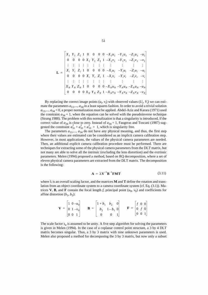
51
By replacing the correct image points (ui, vi) with observed values (Ui, Vi) we can esti-mate the parameters a11,..., a34 in a least squares fashion. In order to avoid a trivial solutiona11,..., a34 = 0, a proper normalization must be applied. Abdel-Aziz and Karara (1971) usedthe constraint a34 = 1, when the equation can be solved with the pseudoinverse technique(Strang 1988). The problem with this normalization is that a singularity is introduced, if thecorrect value of a34 is close to zero. Instead of a34 = 1, Faugeras and Toscani (1987) sug-gested the constraint , which is singularity free.
The parameters a11,..., a34 do not have any physical meaning, and thus, the first stepwhere their values are estimated can be considered as an implicit camera calibration step.However, in most applications, the values of the physical camera parameters are needed.Then, an additional explicit camera calibration procedure must be performed. There aretechniques for extracting some of the physical camera parameters from the DLT matrix, butnot many are able to solve all the intrinsic (excluding the lens distortion) and the extrinsicparameters. Melen (1994) proposed a method, based on RQ decomposition, where a set ofeleven physical camera parameters are extracted from the DLT matrix. The decompositionis the following:
(3.11)
where λ is an overall scaling factor, and the matrices M and T define the rotation and trans-lation from an object coordinate system to a camera coordinate system (cf. Eq. (3.1)). Ma-trices V, B, and F contain the focal length f, principal point (u0, v0) and coefficients foraffine distortion (b1, b2):
The scale factor su is assumed to be unity. A five step algorithm for solving the parametersis given in Melen (1994). In the case of a coplanar control point structure, a 3 by 4 DLTmatrix becomes singular. Thus, a 3 by 3 matrix with nine unknown parameters is used.Melen also proposed a method for decomposing the 3 by 3 matrix, but now only a subset
L
X1 Y 1 Z1 1 0 0 0 0 X1u1– Y 1u1– Z1u1– u1–
0 0 0 0 X1 Y 1 Z1 1 X1v1– Y 1v1– Z1v1– v1–
..
....
..
....
..
....
..
....
..
....
..
....
Xi Y i Zi 1 0 0 0 0 Xiui– Y iui– Ziui– ui–
0 0 0 0 Xi Y i Zi 1 Xivi– Y ivi– Zivi– vi–
..
....
..
....
..
....
..
....
..
....
..
....
XN Y N ZN 1 0 0 0 0 XNuN– Y NuN– ZNuN– uN–
0 0 0 0 XN Y N ZN 1 XNvN– Y NvN– ZNvN– vN–
=
a312 a32
2 a332+ + 1=
A λV 1– B 1– FMT=
V1 0 u0–
0 1 v0–
0 0 1
= B1 b1+ b2 0
b2 1 b1– 0
0 0 1
= Ff 0 0
0 f 0
0 0 1
=

52
of physical camera parameters can be estimated.Since no iteration is required, direct methods are computationally fast. However, such
methods have at least the following disadvantages. First, camera lens distortion cannot bedirectly incorporated, and therefore, the effects of distortion cannot be corrected. Still,some linear solutions to compensate for the radial and tangential lens distortion are present-ed in the literature. For example, Shih et al. (1993) used a method where the estimation ofthe radial lens distortion coefficient is transformed into an eigenvalue problem. Wei andMa (1994) first corrected the lens distortion and then applied a linear calibration methodfor corrected image coordinates.
The second disadvantage cannot be fixed. Due to the objective of composing a noniter-ative algorithm, the actual constraints in the intermediate parameters are not considered.Consequently, in the presence of noise, the intermediate solution does not satisfy the con-straints, and the accuracy of the final solution is relatively poor (Weng et al. 1992).
3.3.4. Multi-step methods
In this section, we concentrate on calibration methods that consist of several successive di-rect and iterative steps. A well-known calibration technique belonging to this category wasdeveloped by Tsai (1987). It is based on the radial alignment constraint (RAC), whichstates that the direction of the vector OP’ extending from the image center O to the imagepoint P’(ui, vi) remains unchanged, and is radially aligned (or parallel) with the vectorextending from the point Po(0, 0, zi) in the optical axis to the point P(xi, yi, zi). This is illus-trated in Fig. 16.
PoP
u
v
x
y
z
P’(ui, vi)
P(xi, yi, zi)
Po(0, 0, zi)
OP’O
X
Y
Z
Fig. 16. Illustration of the radial alignment constraint.
f
PoP

53
There are three important properties of the RAC:
• radial lens distortion does not influence the direction of the vector OP’
• effective focal length f does not influence the direction of the vector OP’
• translation in the direction of the optical axis (z-axis) does not influence the directionof the vector OP’
These properties make it possible to determine a subset of extrinsic parameters (x and ycomponents of translation, 3-D orientation) and the scale factor su by using a linear tech-nique. The rest of the parameters: z component of translation, effective focal length f, anddistortion coefficients k1 (Tsai used only one coefficient) are determined iteratively withnonlinear search. The position of the image center (u0, v0) is assumed to be known in ad-vance or being solved with some separate technique, and the component of tangential dis-tortion in Eq. (3.5) is neglected.
Let us denote the distorted image coordinates in a principal point centered coordinatesystem and . Based on the properties of the RAC listedabove, the following cross product between the vectors OP’ and is written:
(3.12)
Using the transformation in Eq. (3.1) the camera coordinates xi and yi can be expressed interms of object coordinates. We obtain
(3.13)
By treating sum11/y0, sum12/y0, sum13/y0, sux0/y0, m21/y0, m22/y0, and m23/y0, as unknownintermediate variables the following linear model is obtained for N control points:
(3.14)
The coordinates are replaced with corresponding observations and. The set of intermediate variables is then solved in a least squares fashion.
There are nine camera parameters m11, m12, m13, m21, m22, m23, x0, y0, and su in the equa-tion, and seven constraints can be written based on the least squares solution. In addition,based on the orthonormality of the rotation matrix, we know that m11
2 + m122 + m13
2 = 1
uit( ) vi
t( )δ,δ( )
ui' su ui uir( )δ+( )= vi' vi vi
r( )δ+=PoP
ui' su⁄vi'
xi
yi
× 0 or ui'yi suvi'xi– 0= =
ui' m21Xi m22Y i m23Zi y0+ + +( ) suvi' m11Xi m12Y i m13Zi x0+ + +( )=
v1'X1 v1'Y 1 v1'Z1 v1' u1'X1– u1'Y 1– u1'Z1–
..
....
..
....
..
....
..
.
vi'Xi vi'Y i vi'Zi vi' ui'Xi– ui'Y i– ui'Zi–
..
....
..
....
..
....
..
.
vN'XN vN'Y N vN'ZN vN' uN'XN– uN'Y N– uN'ZN–
sum11 y0⁄sum12 y0⁄sum13 y0⁄sux0 y0⁄m21 y0⁄m22 y0⁄m23 y0⁄
u1'
..
.
ui'
..
.
uN'
=
ui' vi',( ) Ui u0–( ) D⁄ uV i v0–( ) D⁄ v

54
and m212 + m22
2 + m232 = 1. Thus, all the parameters involved in Eq. (3.14) can be solved
explicitly.In the second step of the Tsai’s method, the rest of the camera parameters are solved by
using an iterative least squares technique. Now, the search space is reduced to four param-eters. This makes the procedure much lighter than in full-scale optimization. In the case ofa coplanar set of control points, the procedure is slightly different and not all the cameraparameters can be solved, as well as in the DLT technique.
There are some disadvantages in this approach. Firstly, due to the properties of the RAConly radial distortion is handled, and hence, this calibration method cannot be extended totangential distortion. Secondly, the assumption that the principal point is known in ad-vance, is often unfeasible, although there are various techniques that can be applied for lo-cating it separately. A good survey about these techniques was given by Willson and Shafer(1993). However, the methods represented are typically quite inaccurate and they require aspecial hardware setup. Another way to locate the principal point is to minimize the resid-ual of the least squares fit in the first step by adjusting the position of (u0, v0). This proce-dure requires an iterative search, but because there are only two free parameters, a fewiterations are needed to obtain the minimum. This approach was suggested by Lenz andTsai (1988).
The third disadvantage is that the solution is not optimal because the information pro-vided by the image observations has not been fully utilized. The radial component of theimage points are discarded completely, and only the perpendicular components are used forthe solution. As a consequence, the RAC method is very sensitive to noise, especially whenthe angle between the optical axis and the calibration plane is small. According to Batistaet al. (1993) the angle of incidence between the optical axis of the camera and the calibra-tion plane must be at least 30 degrees when a coplanar set of control points is used. Hungand Shih (1990) have shown that the Tsai’s method can be worse than a simple linear meth-od if lens distortion is relatively small.
Batista et al. (1993) suggested a multi-step calibration procedure for coplanar calibra-tion points. The contribution of that work is the computation of the camera look angles (ro-tation matrix). Three look angles expressed in spherical coordinates are obtained by usingonly the 2-D perspective projection of a rectangle of unknown size. With the knowledge ofthe rotation matrix, the translation vector and all the intrinsic parameters can be obtainedbased on an iterative multi-step calculation.
Another multi-step procedure is to first utilize a direct method for obtaining rough esti-mates of the camera parameters, and use them in the second step as initial guesses in full-scale nonlinear minimization. For example, Heikkilä and Silvén (1996b), Weng et al.(1992), and Melen (1994) have applied this schema in their calibration experiments. In gen-eral, a nonlinear optimization algorithm may converge to a local extremum that is not op-timal. However, if a good approximate solution is given as an initial guess, the number ofiterations can be reduced significantly, and the global minimum is reached more reliably.Such a two-step algorithm is more stable than directly starting iteration from an arbitrarilychosen initial guess (Weng et al. 1992). The aspect of the computational load is also not ascritical as it was some years ago, because the current workstations can accomplish the min-imization procedure in a few seconds.

55
3.3.5. Implicit methods
In many cases the explicit values of the physical camera parameters are not necessarily re-quired. For example, in tracking applications only the corrected image coordinates aremeaningful. Therefore, the calibration can be performed without giving any physical inter-pretation for the camera parameters. This kind of approach is called implicit camera cali-bration (Wei & Ma 1994). It should be also noticed that the camera model described inSection 3.2. is only an approximation of the true physical model.
An implicit calibration procedure called the two-plane method was first proposed byMartins et al. (1981). The correct image point was determined by interpolating the calibra-tion points on two calibration planes. This approach has been later developed by Isaguirreet al. (1985) and Wei and Ma (1993, 1994) for example, who generalized the method forany type of lens distortions. The basic idea in the two-plane method is to use a direct trans-formation from image coordinates to world coordinates and vice versa. The world coordi-nates are the intersections of lines of sight on two planes π1 and π2. For example, thetransformation or back-projection from image coordinates (ui, vi) to the coordinates
in the plane π1 can be written as
(3.15)
The set of coefficients are solved in a least squares fashion. The number of the co-efficients depends on the order of the polynomials N. Wei and Ma used third order polyno-mials in their experiments when the number of coefficients become 10 for each polynomial.
The same procedure is repeated for the plane π2, and for the inverse transformation i.e.,projecting the world coordinates to image coordinates. Thus, a total of four sets of coeffi-cients must be solved in order to produce mappings in both directions. The lines of sight inworld coordinates are solved by first projecting the image coordinates to both planes usingthe direct transformations and then calculating the corresponding lines of sights from theintersection points and the known relation between the two planes. The mapping in the op-posite direction is performed by first calculating the projection of the 3-D points on eitherof the planes and then transforming these coordinates to image coordinates.
The advantage of this approach is that a closed form solution exists for both the projec-tion and the back-projection problems. The disadvantage is that more parameters must besolved than in explicit methods. In order to compensate for the increase in the number ofunknowns additional measurements are required.
In the implicit calibration procedure suggested by Faugeras and Toscani (1987) the per-spective transformation matrix is first estimated by neglecting the image distortions. Thereare five intrinsic parameters to be calibrated at this stage that are closely related to the phys-ical parameters, and they can be directly solved by using the perspective transformation. Inorder to compensate for the geometric distortions Faugeras and Toscani composed the im-ages into a number of square buckets in which they assumed that the distortion was homo-geneous and could be modeled by the transformation
Xi Y i,( )
Xi
a jk1( )ui
jvik
0 j k N≤+≤∑
a jk3( )ui
jvik
0 j k N≤+≤∑
-----------------------------------------= Y i
a jk2( )ui
jvik
0 j k N≤+≤∑
a jk3( )ui
jvik
0 j k N≤+≤∑
-----------------------------------------=
a jkn( )

56
(3.16)
where (ui, vi) are the measured pixel coordinates for given control points, and arethe corrected coordinates. The coefficients a, b, c, d, e, f, g and h are found by minimizingthe squared distances between the corrected pixels and the pixels obtained by applying thetransformation matrix to the control point coordinates. The main difficulty in this approachis that the intrinsic parameters calculated in the first stage are not independent of the lensdistortions, and if they are not considered when estimating the perspective transformationmatrix, the camera parameters become inaccurate.
3.3.6. Other methods
In a perspective image, a bundle of 3-D parallel lines are converging into a single point thatis called a vanishing point. During the past few years, camera calibration methods based onthis observation have been proposed, for example, by Caprile and Torre (1990), Echigo(1990), Wang and Tsai (1990), and Beardsley et al. (1992). The basic idea is to use threeorthogonal groups of parallel lines in 3-D space in order to recover some of the intrinsicparameters and the rotation matrix (Li 1994). Beardsley et al. (1992) used a planar set ofparallel lines that were rotated around an axis not perpendicular to the image plane. Basedon the motion of the vanishing points during the rotation, the principal point of the cameracan be located. The advantage of using vanishing points for calibration is that a closed-formsolution for the camera parameters is derived. The disadvantage is that the full set of intrin-sic and extrinsic parameters cannot be obtained, and the accuracy of the method is relative-ly low.
There are also other geometrical methods for detecting the intrinsic camera parameters.For instance, the plumb line method suggested by Brown (1971) uses the images of straightlines for calibrating the lens distortions. Penna (1991a) used an image of a sphere for scalefactor calibration. Lenz and Tsai (1988) proposed a method for scale factor calibrationbased on the observation that the camera signal is formed by superimposition of the idealoutput value representing the image intensity, noise and small signal spikes of the same fre-quency as the camera clock. These spikes are typically suppressed by a low-pass filter, butby removing the filter, the clock frequency can be determined using FFT analysis. Thescale factor is then retrieved from the proportion between the frequencies of the cameraclock and the A/D-converter. There are several methods for calibrating the principal point(image center) that are based on various geometrical and physical properties. A good re-view of these methods can be found from Willson & Shafer (1993).
Also, various methods for calibrating only the extrinsic camera parameters have beenproposed in the literature. Haralick (1989) noticed that there is sufficient information on the2-D perspective projection of a rectangle of unknown size in 3-D space to determine thecamera view angle parameters. Penna (1991b) generalized this approach to the perspectiveprojection of any quadrilateral. Liu et al. (1988) used line and point correspondences to de-termine the camera location. Safaee-Rad et al. (1992) solved the 3-D position and orienta-
u'i a bui cvi duivi+ + +=
v'i e f ui gvi huivi+ + +=
u'i v'i,( )

57
tion problem by using circular features as control points. All of these methods assume thatthe intrinsic camera parameters have already been calibrated. If this is not true, the accuracyof the resulting camera position and orientation can be quite low.
The main problem with most of the methods presented above is that they only considera subset of the intrinsic parameters. In practice, the parameters are coupled in some way,and therefore recovering a single parameter requires that the rest of the parameters are al-ready known. By neglecting their influence, the accuracy of the method can decrease sig-nificantly.
3.4. Inverse model and image correction
The camera model given in Eq. (3.6) expresses the projection of any 3-D point on the imageplane. However, it does not give a direct solution to the back-projection problem, where wewant to recover the 3-D lines of sight from image coordinates. If both radial and tangentialdistortion components are considered, we can notice that there is no analytic solution to theinverse mapping. For example, two coefficients for radial distortion causes the cameramodel in Eq. (3.6) to become fifth order polynomials
(3.17)
We can see from Eq. (3.17) that a nonlinear search is required to recover from. Another alternative is to approximate the inverse model. Weng et al. (1992)
claimed that the distortion model is also an approximation of its inverse. This may be ap-plicable for minor distortion, but in the case of severe errors, a more accurate methodshould be used. Melen (1994) had a similar approach, but instead of using the distortionmodel directly as an inverse transformation, he estimated the undistorted image coordinatesiteratively. He proposed the following two-iteration process:
(3.18)where vectors and contain the distorted and the corrected image coordinates respec-tively. The function represents the distortion in image location q. In our tests (see Fig.32), Melen’s method gave a maximum residual of about 0.12 pixels for typical lens distor-tion parameters. This may be enough for some applications, but if greater accuracy is need-ed then more iterations should be accomplished.
Some implicit methods, e.g. the two-plane method proposed by Wei and Ma (1993,1994), solve the back-projection problem by determining a set of non-physical parametersto compensate for the distortion. Due to a large number of unknown parameters, this tech-nique requires a dense grid of observations from the whole image plane in order to becomeaccurate. However, if we know the physical camera parameters based on explicit calibra-
ui = Dusu k2ui5 2k2ui
3vi2 k+ 2uivi
4 k1ui3 k+ 1uivi
2+ +(
+ 3 p2ui2 2 p1uivi p+ 2vi
2+ui ) u0+ +
vi = Dv k2ui4vi 2k2ui
2vi3 k+ 2vi
5 k+ 1ui2vi k+ 1vi
3+(
+ p1ui2 2 p2uivi 3 p1vi
2 vi )+ + + v0+
ui vi,( )ui vi,( )
qi' qi'' δ qi'' δ qi''( )–( )–=
qi'' qi'δ q( )

58
tion, it is possible to solve the unknown parameters of Eq. (3.15) by generating a dense gridof points and calculating the corresponding distorted image coordinates us-ing the camera model in Eq. (3.6). Now, we can express the mapping from to
by treating the image plane as a calibration plane π1:
(3.19)
Wei and Ma used the third order polynomials in their experiments. However, it is quiteclear that a ratio of two third order polynomials does not provide adequate approximationfor the inverse of the fifth order polynomial in Eq. (3.17). Thus, at least fifth order approx-imations should be applied. This leads to equations where each set of unknown parameters
includes at least 21 terms. It can be expected that there are also redundant parame-ters that can be eliminated. Using backward elimination (Draper & Smith 1981) the numberof parameters was reduced step by step, and it was observed that the following eight param-eter model compensated for the lens distortions so that the maximum residual error was al-ways less than 0.01 pixels even with severe distortion:
(3.20)
where , , and . If we comparethis result to the camera model in Eq. (3.6), we notice that also the inverse model has radialand tangential components. The counterparts for the distortion parameters k1, k2, p1, and p2are the coefficients a1,..., a4. The inverse distortion model contains only eight unknown pa-rameters instead of 63 parameters that were in the original model in Eq. (3.19). Clearly,evaluating this model will require less computation than the iterative approach suggestedby Melen.
In order to solve the unknown parameters a1,..., a8 N tie-points andcovering the whole image area must be generated. The distorted image coordinates
are derived by adding the lens distortion to true coordinates . The lens dis-tortion is computed from the camera model in Eq. (3.6). In practice, a grid of about 1000 -2000 points, e.g. 40 by 40, is enough. The parameters a1,..., a8 are then solved by using di-rect least squares fitting. Let us define the following matrix T and vectors p and e:
ui vi,( ) ui vi,( )ui vi,( )
ui vi,( )
ui
a jk1( )ui
jvik
0 j k N≤+≤∑
a jk3( )ui
jvik
0 j k N≤+≤∑
-----------------------------------------= vi
a jk2( )ui
jvik
0 j k N≤+≤∑
a jk3( )ui
jvik
0 j k N≤+≤∑
-----------------------------------------=
a jkn( )
ui
ui' ui' a1ri2 a2ri
4+( ) 2a3ui'vi' a4 ri2 2ui'
2+( )+ + +
a5ri2 a6ui' a7vi' a8+ + +( )ri
2 1+-------------------------------------------------------------------------------------------------------------------=
vi
vi' vi' a1ri2 a2ri
4+( ) a3 ri2 2vi'
2+( ) 2a4ui'vi'+ + +
a5ri2 a6ui' a7vi' a8+ + +( )ri
2 1+------------------------------------------------------------------------------------------------------------------=
ui' ui u0–( ) Dusu( )⁄= vi' vi v0–( ) Dv⁄= ri ui'2 vi'
2+=
ui vi,( ) ui' vi',( )
ui' vi',( ) ui vi,( )

59
Using T, p and e Eq. (3.20) can be written in the matrix form
(3.21)
The vector p is now estimated in a least squares sense by applying a pseudoinverse tech-nique
(3.22)where T+ denotes the pseudoinverse (Strang 1988) of the matrix T.
The parameters computed with Eq. (3.22) are then used in Eq. (3.20) to correct arbitraryimage coordinates (ui, vi). It should be noticed that the inverse distortion model is only anapproximation and the parameters do not have any physical meaning. Therefore, it can bealso considered as an implicit calibration step. What is actually done in the image correc-tion is interpolation between the tie-points.
3.5. Measurement error sources
The importance of data acquisition and its accuracy has often been ignored in the literaturealthough it has a key role when evaluating the results. Systematic errors in the optimizationresidual indicate either shortcomings in the camera model or problems in data acquisitionfor camera calibration.
The main error source that is often considered is the quantization noise. This is causedby the finite spatial resolution of the CCD array, sampling of the video signal, and signalquantization to some predefined levels. Small features may vanish or their location can bebiased due to quantization, but points much larger than a single pixel can be detected quiteaccurately. Based on the central limit theorem, it can be assumed that the measurementnoise distribution is asymptotically normal. Moreover, the accuracy can be improved by
T
u1'r12– u1'r1
4– 2u1'v1'– r12 2u1'
2+( )– u1r14 u1u1'r1
2 u1v1'r12 u1r1
2
v1'r12– v1'r1
4– r12 2v1'
2+( )– 2u1'v1'– v1r14 v1u1'r1
2 v1v1'r12 v1r1
2
..
....
..
....
..
....
..
....
ui'ri2– ui'ri
4– 2ui'vi'– ri2 2ui'
2+( )– uiri4 uiui'ri
2 uivi'ri2 uiri
2
vi'ri2– vi'ri
4– ri2 2vi'
2+( )– 2ui'vi'– viri4 viui'ri
2 vivi'ri2 viri
2
..
....
..
....
..
....
..
....
uN'rN2– uN'rN
4– 2uN'vN'– rN2 2uN'2+( )– uNrN
4 uN uN'rN2 uN vN'rN
2 uNrN2
vN'rN2– vN'rN
4– rN2 2vN'2+( )– 2uN'vN'– vNrN
4 vN uN'rN2 vN vN'rN
2 vNrN2
=
p a1 a2 a3 a4 a5 a6 a7 a8, , , , , ,,[ ]T=
e u1' u1 v1' v1 … ui' ui vi' vi … uN' uN vN' vN–,–, ,–,–, ,–,–[ ]T=
e Tp=
p T+e=

60
averaging the detected feature position from several images. This is an ideal assumptionthat fits well to the noise requirements of the least squares estimators. However, it is typi-cally valid only up to a certain limit, and below that limit other error sources become dom-inant.
As we noticed in Chapter 2., the feature extraction process can introduce additional er-rors that are usually systematic. For instance, direct ellipse fitting by minimizing the alge-braic distance is slightly biased. There can be a small number of outliers present in themeasurement data due to various reasons. These outliers may cause significant errors in theleast squares estimation process. They should therefore be eliminated or some robust esti-mation techniques (Huber 1981, Hampel et al. 1986) should be used. There are also othertypes of errors that are discussed in the following sections.
3.5.1. Hardware
The adjacent pixels on the image sensor are separated by narrow isolation regions that re-duce the measurement accuracy. The size of the gap depends on the image plane architec-ture, e.g. the interline transfer cameras have a reasonably large gap between adjacenthorizontal lines. Especially for line shaped features, this may cause problems, because verynarrow objects vanish or their location is distorted.
The charges accumulated under the photosensitive cells are typically converted to an an-alog video signal, where the picture information is transmitted serially. The conversion ofthe two-dimensional image into a one-dimensional electrical signal is accomplished byraster scanning. In order to reconstruct the image, additional information is needed to syn-chronise the frame grabber. This information called horizontal and vertical sync pulses isincluded within the video signal. Using the phase locked loop (PLL) the frame grabber triesto reconstruct the camera’s pixel clock by generating a stable reference clock which is syn-chronized to the horizontal sync pulses of the video signal. However, this process producesa certain amount of deviation with respect to the correct pixel clock. This deviation is calledline jitter and it causes timing errors of a few nanoseconds, typically 5 - 20 ns peak to peak,that correspond to around 1/16 - 1/4 pixels noise in horizontal line direction. The noise isoften random, but sometimes it may cause systematic shifting in different parts of the imagedue to instability in PLL operation. Methods for detecting and compensating for the linejitter are discussed in Beyer (1990). Compensating for the systematic jitter requires addi-tional calibration steps. The image can either be resampled or the coordinates of the fea-tures of interest corrected.
The CCD arrays are manufactured with high precision. The deviations in coplanarityand collinearity have been shown to remain below 1/100 pixels (Haggrén 1989). Theorthogonality error of the array is sometimes included in the camera model (e.g. Melen1994), but typically it is neglected due to its insignificance.

61
3.5.2. Calibration target
There are many ways of implementing the calibration target. It can be coplanar, three-di-mensional, solid, transparent, etc. The size of the target depends on the dimensions of theobject space to be measured. In the ideal case, it should cover the entire object space. Thiscan be arranged by placing a set of reference points in the object space. These points arethen measured with an external coordinate meter, and used in the calibration procedure ascontrol points. However, in many cases it is not possible to use external devices that areaccurate enough. Self-calibration is one solution, another is a movable target. For practicalreasons, the target cannot be very large. It must therefore be used in shorter distances thanthe actual measurement setup would demand in order to cover the entire image.
The 3-D accuracy of the calibration target should be checked before starting calibration.The errors in the control point coordinates can cause the results to be unsatisfactory, be-cause the calibration accuracy cannot be better than the precision of the target. For exam-ple, if the desired proportional accuracy is 1/10000, the standard error in control pointcoordinates cannot be larger than 0.05 mm for the entire target volume whose principal di-mension is 500 mm. This requirement is very difficult to be achieved without high preci-sion tools. Using a laser printer to create a dot pattern is simply not adequate for suchaccuracies. In addition, the flatness of the target should be ensured in the case of planar tar-gets.
3.5.3. Projection asymmetry with circles
Perspective projection is generally not a shape preserving transformation. Only lines aremapped as lines on the image plane. Two- and three-dimensional shapes with non-zero pro-jection area are transformed if they are not coplanar with the image plane. This is true forarbitrary features, but in this context we are only interested in circles, because of their sim-ple mathematic formulation. They are also very common in many man-made objects.
Circles have been often used in camera calibration (e.g. Shih et al. 1995, Lenz & Tsai1988, Han & Rhee 1992, Wei & Ma 1993, Melen 1994) and in 3-D location estimation (e.g.Kabuka & Arenas 1987, Gårding & Lindeberg 1994, Buurman 1992, Magee & Aggarwal1984). The center points of the circles are often located from the images with subpixel pre-cision, but the distortion caused by the perspective projection is not typically considered.
Perspective projection distorts the shape of the circular features in the image planedepending on the angle and displacement between the object surface and the image plane.Only when the surface and the image plane are parallel, projections remain circular. Thesefacts are well-known, but the mathematical formulation of the problem has been often dis-regarded. We shall therefore next review the necessary equations.
Let the coordinate system Ω1 (X, Y, Z) ∈ ℜ3 be centered in the camera focus O, and letits Z axis be perpendicular to the object surface Π1 (see Fig. 17). The rays coming from thecircle Γ1 that is placed on the surface Π1 form a skewed cone, whose boundary curve C isexpressed as follows:
(3.23)X αZ–( )2 Y βZ–( )2+ γ 2Z2=

62
Parameters α and β specify the skewness of the cone in X and Y directions and the param-eter γ specifies the sharpness of the cone. Thus, if the distance from the camera focus to theobject surface is denoted by d, the circle equation becomes (X - αd)2 + (Y - βd)2 = (γd)2.
The camera coordinate system Ω2 (x, y, z) ∈ ℜ3 is also centered in the camera focus, butits z-axis is orthogonal to the image plane Π2, and the x- and y-axes are parallel to the imagecoordinates. Thus, the transformation from Ω2 to Ω1 can be expressed by using rotation
(3.24)
where the vectors , , and form an orthonor-mal basis.
Now we can express Eq. (3.23) in camera coordinates:
(3.25)
Let us denote the focal length, i.e. the orthogonal distance between O and Π2, by f. Then,the intersection Γ2 of C and Π2 is given by the equation
(3.26)
O
Z
X Y
Π1
Γ1
Γ2
C
p
Π2
Fig. 17. Perspective projection of a circle.
X
Y
Z
a11 a12 a13
a21 a22 a23
a31 a32 a33
x
y
z
=
a11 a21 a31, ,[ ]T a12 a22 a32, ,[ ]T a13 a23 a33, ,[ ]T
a11 αa31–( )x a12 αa32–( )y a13 αa33–( )z+ +[ ]2
+ a21 βa31–( )x a22 βa32–( )y a23 βa33–( )z+ +[ ]2
γ 2 a31x a32y a33z+ +( )2=
n2 k2 r2–+( )x2 2 kl np rs–+( )xy l2 p2 s2–+( )y2+ +
2 km nq rt–+( )x 2 lm pq st–+( )y m2 q2 t2–+ + + + 0=

63
where
We notice from Eq. (3.26) that projection is a quadratic curve and its geometrical interpre-tation can be a circle, hyperbola, parabola, or ellipse. In practice, due to the limited field ofview, the projection will be a circle or an ellipse.
Based on Eq. (3.26) the center of the ellipse becomes
(3.27)
In order to find out what is the projection of the circle center, let us consider a situationwhere the radius of the circle is zero, i.e. γ = 0. Consequently, r, s, and t become zero, andwe obtain the position of the projected point that is, due to the symmetry of the circle, alsothe projection of the true circle center :
(3.28)
For non-zero radius (γ > 0) there are only some special cases when Eqs (3.27) and (3.28)are equal, e.g. the rotation is performed around the Z-axis (a31 = a32 = 0). Generally, wecan state that the ellipse center and projected circle center are not the same for circular fea-tures with non-zero radius.
Ellipse fitting and the center of gravity method produce estimates of the ellipse center.However, what we usually want to know is the projection of the circle center. As a conse-quence of the previous discussion, we notice that the estimate is biased and it should be cor-rected using Eqs (3.27) and (3.28). Especially in camera calibration, this is very importantbecause the circular dot patterns are usually determined in skewed angles, and without cor-rection the parameters become erroneous.
There are at least two possibilities for correcting the problem. The first solution is to in-clude the correction in the camera model. An unbiased and minimumvariance estimate in a least squares sense is then obtained. However, this solution decreasesthe convergence rate and thus, increases the amount of computation. Another possibility isto compute the camera parameters in multiple steps. In the calibration procedure proposedby Heikkilä & Silvén (1996b), the initial camera parameters are computed with the DLTtechnique by neglecting the nonlinear distortion components. In the second stage, the reg-ular nonlinear minimization is performed by using the camera model of Eq. (3.6). In the
k a11 αa31–=
l a12 αa32–=
m a13 αa33–( ) f=
n a21 βa31–=
p a22 βa32–=
q a23 βa33–( ) f=
r γ a31=
s γ a32=
t γ a33 f=
uc vc,( )
uckp nl–( ) lq pm–( ) ks lr–( ) tl ms–( )– ns pr–( ) wp qs–( )–
kp nl–( )2 ks lr–( )2– ns pr–( )2–----------------------------------------------------------------------------------------------------------------------------------------------------=
vckp nl–( ) mn kq–( ) ks lr–( ) mr kt–( )– ns pr–( ) qr nt–( )–
kp nl–( )2 ks lr–( )2– ns pr–( )2–---------------------------------------------------------------------------------------------------------------------------------------------------=
uo vo,( )
uolq pm–kp nl–-------------------=
vomn kq–kp nl–-------------------=
uc uo vc vo–,–( )

64
last stage, Eqs (3.27) and (3.28) are evaluated based on the existing camera parameters andthe observations (Ui,Vi) are corrected with the following formula:
(3.29)
After this correction, the camera parameters are recomputed. The parameters are not opti-mal in a least squares sense, but the remaining error is typically so small that further itera-tions are not necessary.
In Fig. 18a, there is an image of a cubic 3-D object. Since the two surfaces are perpen-dicular to each other, there is no way of selecting the viewing angle so that the error causedby the projection asymmetry vanishes. Fig. 18b and Fig. 18c show this error in the imagecoordinates both in horizontal and vertical directions. The error in this case is quite small(about 0.12 pixels peak to peak), but it is systematic causing bias to the camera parameters.
3.5.4. Illumination
In a lens system, the illumination of the image plane will be found to decrease away fromthe optical axis at least with the 4th power of the cosine of the angle of obliquity with theoptical axis (Willson & Shafer 1993). This fall-off may cause the intensity profile of thefeature to be distorted as can be noticed from Fig. 13c. The error in the observed locationof the feature depends considerably on the feature extraction technique used. For the inten-sity weighted center of gravity (CoG) method (Section 2.4.6.) the effect of the radiometricfall-off may be more significant than for edge fitting based methods.
However, our tests have shown that changing the lighting conditions has a more exten-sive effect on the point locations than the cos4th law of the radiometric fall-off could ex-plain. In Fig. 19a there are two images captured from exactly the same position and angleusing the same camera settings, and only the overall lighting has changed from fluorescentto halogen light. The nominal focal length of the optics is 8.5 mm. Fig. 19b shows the dif-ference between the detected control point locations in the image plane. The difference issmallest near the image center and increases radially when approaching the image borders.From Fig. 19c we notice that the difference is almost linear as a function of the horizontaland vertical coordinates. This type of variation is therefore compensated for by a smallchange in the focal length of the pinhole camera model. As a consequence, the error cannotbe detected from the residue of the optimization process.
In the case of Fig. 19, the focal length seemed to change by about 20 µm (0.2%). Thesame phenomenon was observed with several CCD cameras and lenses. However, it wasnoticed that the magnitude of the variation mainly depends on the focal length. Typically,short optics (f < 10 mm) gave larger disparity than long optics (f > 20 mm). An obviousreason for this effect is the chromatic aberration. According to Smith and Thomson (1988)chromatic aberration is a measurement of the spread of an image point over a range ofcolors. It may be represented either as a longitudinal movement of an image plane, or as achange in magnification, but basically it is a result of the dependence of the power of a re-fracting surface on wavelength.
Ui' Ui Dusu uc i, uo i,–( )–=
V i' V i Dv vc i, vo i,–( )–=

65
The spectral power of the fluorescent lamp is centered close to the blue end of the visiblelight spectrum, whereas the halogen lamp spectrum is close to the infra-red region. Due tothe slightly different refraction properties of the camera optics for those wavelengths, thefocal length is also changed. The refraction in short optics is more drastic than in long op-tics, which explains the changes with different focal lengths. This variation is mainly avoid-ed by using high quality achromatic optics or a mono-chromatic filter in front of the camerawhich passes only a narrow band of the light spectrum to the camera optics. Due to the re-duced intensity of the light transmitted through the filter to the image sensor, the integrationtime should be increased.
Another type of measurement error can also be distinguished from Fig. 19c: the horizon-tal shift of the observed feature locations. This shift is caused by a change in the overall
Fig. 18. (a) A view of the calibration object, and the corresponding error in observed (b) hori-zontal and (c) vertical image coordinates caused by the projection asymmetry. The error isrepresented with respect to the feature locations in the image.
(a)
(b) (c)
0.08
0.06
0.04
0.02
0
-0.02
-0.04
-0.06
-0.080 100 200 300 400 500 600 700
u-axis [pixels]
Err
or [p
ixel
s]
0.08
0.06
0.04
0.02
0
-0.02
-0.04
-0.06
-0.080 100 200 300 400 500 600 700
v-axis [pixels]
Err
or [p
ixel
s]

66
intensity of lighting. In Fig. 19a the left image is less exposed than the right image. FromFig. 19c it can be noticed that a shift of about -0.15 pixels has occurred as the intensity hasincreased. In this case, the shift is compensated for by a small change in the principal pointlocation. However, the same phenomenon occurs also if the surfaces of the object are notuniformly illuminated, causing variation in the amount of shifting in different parts of theimage. This variation is not entirely compensated for by the camera model, and therefore itcan be detected from the increased residual error of the calibration procedure. As a result,uniform lighting of the target should be provided in order to guarantee successful cameracalibration. In practice, uniform lighting is very difficult to produce on perpendicular sur-faces as in Fig. 19. The same problem also exists with planar 2-D objects when the camera
(a)
(b) (c)
Fig. 19. (a) Calibration object under two different light sources: a fluorescent lamp on the leftand a halogen lamp on the right. (b) and (c) Difference (phalogen - pfluorescent) between detectedfeature locations.
0 50 100 150 200 250 300 350 400 450 500
0 50 100 150 200 250 300 350 400 450 500
0.4
0.2
0
-0.2
-0.4
-0.6
0.4
0.2
0
-0.2
-0.4
-0.6
u-axis [pixels]
v-axis [pixels]
Diff
eren
ce [p
ixel
s]D
iffer
ence
[pix
els]
50
100
150
200
250
300
350
400
450
500100 200 300 400 500

67
position is changed between the images, causing variation in the amount of light perceivedin different angles. In this case, the error is not necessarily observable in the residue, be-cause it is mainly compensated for by the basic camera model. The reason for this phenom-enon is not exactly known, but one possible source is line jitter (see Section 3.5.1.), becausea change in the intensity of light may affect the PLL operation, producing systematic vari-ation in the sampling rate. According to Beyer (1990) detection of sync pulses is level sen-sitive and influenced by any changes in the signal level. This problem can be reduced byusing a frame grabber with a low jitter characteristic and external sync pulses obtained di-rectly from the camera.
These illumination based problems limit the accuracy and operational environment of acamera based 3-D measurement system. First-class results can be obtained only in the samelighting conditions as those used in calibration. Additionally, when using a moving camera,the light perceived will always change slightly during the sequence. Therefore, the cameramotion should be as short as possible. The 3-D reconstruction procedure suggested inChapter 4. operates with short translational camera motion, and therefore, it meets this con-dition.
3.5.5. Focus and iris
The camera model in Eq. (3.6) is based on a pinhole projection, and it does not consider theeffect of focus and the iris adjustments. It is therefore necessary to determine, how thesesettings can affect the calibration results. In the case of camera focusing, the distance be-tween the image plane and the principal plane of the optics is adjusted in order to sharpenthe image. Clearly, this operation affects the effective focal length of the camera, but it mayalso change other parameters. In Fig. 20a, there is an example of how the adjustment frominfinity to 0.5 m distance can affect the feature locations. The white arrows show the direc-tion and the proportional magnitude of the change. The maximum change in the image co-ordinates of the circles is about five pixels. The image is expanded, which means that thefocal length has become longer. However, the center of the expansion is not in the middleof the image. This is a sign of a small shift in principal point coordinates. More profoundexamination showed that only the focal length and the principal point location was notablychanged, and the radial and tangential components of lens distortion remained almost un-changed. Quite similar results were obtained by Li (1994), who tested the effect of focus-ing, zooming and iris adjustment on principal point location and focal length using theKTH-head-eye system.
In the case of iris opening and closing, Li reported that no significant change in the focallength occurs. However, if we look at Fig. 20b, where two images with different iris set-tings have been captured, we notice from the arrows a systematic change in feature loca-tions. The effect is very similar to focusing, although the magnitude of the disparity is muchsmaller. In this case, the maximum change is about 0.5 pixels. The shift in principal pointlocations is also not as significant as in focusing. However, these results cannot be gener-alized, because they depend very much on the lens and the aperture configuration of theoptics. The calibration should therefore be performed for those settings that correspond tothe conditions in the actual measurement stage.

68
3.6. A calibration procedure for circular control points
Based on the previous discussion, a four-step calibration procedure (Heikkilä & Silvén1997) is suggested. It consists of three steps for estimating the physical camera parameters.The fourth step is needed for solving the back-projection problem. In the first stage, the di-rect linear transform (DLT) is applied to estimate the camera parameters (Section 3.3.3.).These values are then used in the second step as a starting point for the nonlinear search(Section 3.3.1.). The third step is needed if the control points are circular and their projec-tions in the image plane cover regions of several pixels (Section 3.5.3.). In this step, the cor-rections for the observations are first calculated based on Eq. (3.29), and then theparameters are recomputed using the corrected observations. If the projection areas of thecontrol points are small, the third step can be skipped.
The fourth step of the procedure solves the image correction and the back-projectionproblem (Section 3.4.). Image correction is performed by using the inverse distortion modelin Eq. (3.20). Using this model makes the distortion correction process very fast withoutreducing the accuracy. The parameters of the inverse model are computed based on thephysical camera parameters obtained during the first three steps. After distortion correc-tion, the lines-of-sight in 3-D space can be easily reconstructed.
Fig. 20. The effect of (a) focus, and (b) iris adjustments on feature locations.
(a) (b)

69
3.7. Discussion
Geometric camera calibration is necessary when high accuracy in the 3-D reconstructionprocess is desired. A lot of research has been done in this field for a long time. As an indi-cation of that, several camera calibration techniques have been suggested especially incomputer vision literature. Most of these techniques have concentrated on reducing thecomputational intensity of the classical method, at the cost of decreased accuracy, however.Thus the most significant contribution of these methods is that they produce a good startingpoint for nonlinear search. The computational intensity of the classical method no longerplays such an important role, because modern computers can solve the camera parametersin a few seconds, assuming that a good initial guess is available.
The camera calibration literature does not pay much attention to the errors originatingin the calibration process. There are several error sources that may affect the accuracy ofthe estimated camera parameters. Some of the errors are caused by the insufficient cameramodel and others are due to some external factors. The commonly used camera model com-pensates for only radial and tangential lens distortions. It does not consider the effect of thelight intensity, wavelength, focus, iris, electrical distortions, etc. These sources shouldtherefore be identified through other means and some actions for preventing their influenceshould be made. For example, by using a mono-chromatic filter in front of the camera wecan reduce the influence of the chromatic aberration. Also some external factors, like out-liers in measurements, inaccurate calibration target, and asymmetric feature projection, cancause bias in camera parameter estimates.
A four-step procedure for camera calibration was presented in this chapter. This proce-dure can be utilized in various machine vision applications, but it is most beneficial in cam-era based 3-D measurements and in robot vision, where high geometrical accuracy isneeded. This procedure uses explicit calibration methods for computing physical cameraparameters. The mapping from image coordinates to lines-of-sight is performed by usingan inverse distortion model, whose parameters are solved in the fourth step of the calibra-tion procedure.

4. Motion estimation and 3-D reconstruction
4.1. Introduction
In this context, camera motion is understood as a camera displacement between consecu-tive image frames in an image sequence, and 3-D reconstruction is the process of estimatingthe mutual location of the features in a static 3-D environment. Estimation of the cameramotion and the 3-D structure are closely related to each other, because the structure cannotbe determined without first knowing the relative camera locations. For a fixed, two camerastereo system, only one displacement vector consisting of translation and rotation compo-nents must be determined in system calibration. In the case of a moving camera, motionestimation must be performed based on image correspondences. Thus, increasing thenumber of features will improve the accuracy of the motion estimates, and consequently,the accuracy of the estimated 3-D structure.
One of the most difficult problems in multi-camera based vision is the feature corre-spondence problem. In order to achieve proper accuracy with a minimal number of camer-as, it is desirable to have long base-lines, which means that cameras should be placed as farfrom each other as possible. As a consequence, the large disparity between the images oftencauses difficulties in feature matching. Using epipolar lines the search space can be limitedto a narrow band, but, due to the large disparity, the shape of the features may be quite dif-ferent. Partial or total occlusion of the features is also often troublesome.
The feature correspondence problem can be mainly solved by tracking the feature tra-jectories in an image sequence. If the disparity between images is small it is often possibleto detect corresponding features from successive frames simply by selecting spatially theclosest features as pairs. The tracking process may also be improved by introducing a pre-dictive tracker that utilizes information from previous frames to predict the position of fea-tures in the following frame. Kalman filtering is a typical solution for the trackingproblems.
There are basically two approaches for computing motion and 3-D structure from imagesequences if the 2-D feature correspondences are already known. In the sequential ap-proach, computation is performed frame-by-frame consecutively so that the estimates forboth motion and structure are improved by integrating data with an optimal filter. In the

71
batch approach, the measurements are processed simultaneously with some numerical op-timization technique. Clearly, the former approach is computationally lighter, but it hasbeen shown by Weng et al. (1993) that the batch technique produces more accurate motionand 3-D estimates. Generally, in both cases a nonlinear estimation technique is required.However, there are also some closed-form solutions to the problem, but these techniquesare either sub-optimal or constrained.
The problem for obtaining structure from motion has received a lot of attention duringthe past few decades, and a variety of estimation techniques have been proposed in the lit-erature. In this chapter, some of the most important methods are first reviewed, and then, aclosed-form solution to the motion estimation problem in the case of pure translationalcamera movement is presented. Finally, a framework and an accuracy analysis for a camerabased 3-D measurement system is introduced that utilizes translational camera motion andlinear estimation techniques.
4.2. 3-D shape from a single view
Before going to multi-frame methods, we will briefly discuss about inferring 3-D informa-tion from a single view. Due to projective mapping, it is generally impossible to determine3-D coordinates of a feature from a single 2-D image. However, by introducing some con-straints to the imaging arrangements, partial or full reconstruction becomes possible. Thebasic idea of monocular vision is to understand in which situations and under which condi-tions a single 2-D image can provide enough information for a 3-D interpretation of thescene. A set of paradigms, known as “shape from X” has been developed within this refer-ence, such as shape from shading, shape from texture, and shape from contours (Ferri et al.1993). Also, a single camera based active triangulation, or structured lighting technique,belongs to this category. The shape is then reconstructed from light stripes or grid patternsusing the known geometry between the light source and the camera.
Shape from contours is closely related to the topic of this thesis. As we know lines areprojected as lines, and circles are projected as ellipses in the image plane, and their explain-ing parameters can be recovered very accurately by using subpixel edge detection and theadvanced fitting techniques discussed in Chapter 2. Several methods have been proposedfor estimating 3-D information from these parameters. For example, Ferri et al. (1993) han-dled the perspective inversion of the following configurations: four coplanar line segments,three orthogonal line segments, a circle arc, and a quadratic of revolution. Haralick et al.(1984) estimated the position and orientation of a wire frame object based on camera pro-jections. Safaee-Rad et al. (1992) proposed a closed-form solution for estimating 3-D po-sition and orientation of a circular feature from a single image.
If the mutual 3-D relationships between the features are known in advance, camera po-sition and orientation with respect to the object coordinates can be determined from a singleview. Depending on the number of point features, these techniques are subdivided into a 3-point problem, also called the triangle-pose problem (e.g. Linnainmaa et al. 1988), a 4-point problem (e.g. Horaud et al. 1989), and an n-point problem (e.g. Haralick & Joo 1988).Analytic solutions exist for the first two problems. In the n-point problem, the set of pro-jection equations is over-determined, and therefore, some statistical method, like the least

72
squares fitting, must be applied. Analytic solutions are computationally fast, but due tomeasurement errors in the observed image coordinates they do not provide very accurateresults. Besides, closed-form solutions to the n-point problem exist (e.g. Ganapathy 1984).
Single view based methods are often considered as separate techniques with respect tomulti-view approaches, because the multi-view techniques typically utilize only the paral-lax between different views. Using the extra information provided by contours, textures,etc. would improve the accuracy of the 3-D estimates also in the multi-view approaches.However, this possibility is not considered in the next sections due to the increased com-plexity of the solutions.
4.3. Kalman filtering
Kalman filtering (Kalman 1960) is a well-known technique for solving state estimationproblems in control systems theory. It has been also widely used in computer vision fortracking and vision based control of dynamic systems (visual servoing). For example,Dickmanns and Graefe (1988) listed the following four different application areas for ex-tended Kalman filter based monocular machine vision: balancing of an inverted pendulum,vehicle docking, road vehicle guidance, and aircraft landing approach. For 3-D location andmotion estimation of a known rigid object it has been applied e.g. by Wu et al. (1988). Inaddition to the camera position and motion parameters Silvén & Repo (1993) and Röninget al. (1994) estimated also the structure of the unknown scene from image sequence. Theyused a two-step filtering approach, where motion and structure were estimated separatelywith different state models. The same approach was the basis in the study performed byHeikkilä and Silvén (1995, 1996a), where the feasibility of this technique for accurate 3-Dmeasurements was tested.
4.3.1. Motion estimation
As we noticed in Section 4.2., the 3-D position of the camera with respect to some fixedcoordinate frame can be recovered from a single image, if the scene structure is known inadvance. As a consequence, the motion between distinct frames can be also estimated basedon feature correspondences. The problem is how much confidence we can have in thesemeasurements and can we somehow utilize the information from previous frames. It can beoften assumed that the camera motion is smooth and sudden changes in its direction andvelocity are not expected. Based on this assumption, a dynamic state-space model of thecamera motion between discrete time instants k and k + 1 is expressed as
(4.1)
The state vector contains camera posi-tion (xk, yk, zk) and orientation (ωk, ϕk, κk) parameters and corresponding velocities at theinstant k. The meaning of these parameters is illustrated in Fig. 14. The matrix Φk, k + 1 is
xk 1+ Φk k 1+, xk εk+=
xk xk xk yk yk zk zk ωk ωk ϕk ϕk κk κk, , , , , , , , , , ,[ ]T=

73
a state transition matrix that describes the mapping between consecutive states. It is definedas follows:
where T is the time interval between successive states. Vector εk is a 12 by 1 noise vectorthat models the random variation in the state variables. It is assumed in Eq. (4.1) that thevariation is white Gaussian noise with covariance matrix .
Here, we only use the 2-D image coordinates of the feature locations as measurements,although some other properties, like ellipse geometry, can be also utilized to give extra in-formation. We noticed in Section 3.2. that the transformation from the object coordinatespi = [Xi, Yi, Zi]
T to the image coordinates qi = [ui, vi]T is a nonlinear function. Let us denote
this transformation at the instant k by qi,k = F(pi, xk). Now, we can write the followingequation for the image observation zi,k of the point pi:
(4.2)
The vector ηi,k represents the measurement error. As well as state variable noise, the meas-urement error is also assumed to be white Gaussian noise with covariance matrix
.From Eqs (4.1) and (4.2) we need to construct a procedure for determining the camera
position and velocity at different time instants by weighting the current measurements andprevious states in an optimal manner. The Kalman filter (Kalman 1960) is an optimal re-cursive state estimator that uses information from both the state equation and the measure-ment equation. It minimizes the mean squared error between the observations and a linearmodel. However, in this case the measurement model is nonlinear, and therefore, we mustuse the extended Kalman filter (EKF) that linearizes the measurement model around thecurrent state estimate.
The extended Kalman filter time update equations for the state vector and the estimationcovariance matrix Qk representing the uncertainty of the state estimate are
(4.3)
Φk k 1+,
1 T 0 0 0 0 0 0 0 0 0 0
0 1 0 0 0 0 0 0 0 0 0 0
0 0 1 T 0 0 0 0 0 0 0 0
0 0 0 1 0 0 0 0 0 0 0 0
0 0 0 0 1 T 0 0 0 0 0 0
0 0 0 0 0 1 0 0 0 0 0 0
0 0 0 0 0 0 1 T 0 0 0 0
0 0 0 0 0 0 0 1 0 0 0 0
0 0 0 0 0 0 0 0 1 T 0 0
0 0 0 0 0 0 0 0 0 1 0 0
0 0 0 0 0 0 0 0 0 0 1 T
0 0 0 0 0 0 0 0 0 0 0 1
=
W E εkεkT( )=
zi k, F pi xk,( ) ηi k,+=
V E ηi k, ηi k,T( )=
xk 1 k+ Φk k 1+, xk k=

74
(4.4)
The nonlinearity of the measurement model requires more attention. First, we need to lin-earize the transformation function F by applying the first order Taylor expansion. As a re-sult we obtain the following Jacobian matrix:
(4.5)
The Jacobian matrix is obtained by differentiating the measurement function with respectto the state variables. Either an analytic solution or a numeric approximation must be used.Analytic expressions of the derivatives for a pure pinhole camera model are given bySchwidefsky and Ackermann (1976) for example.
The measurement update equations for the EKF in covariance form are
(4.6)
(4.7)
(4.8)
where , , I is an identity matrix, and Nis the number of the features. The matrix Kk is called Kalman gain.
Unlike the linear Kalman filter, the extended Kalman filter is not guaranteed to be opti-mal, and therefore, it does not always give the minimum mean square solution. In order toachieve better estimation accuracy, we may need to iterate Eqs (4.5)-(4.8) as discussed byGelb (1974) and Broida & Chellappa (1986). The following iterated extended Kalman filter(IEKF) measurement update equations are obtained from Broida & Chellappa (1986):
(4.9)
(4.10)
(4.11)
(4.12)
The iteration is started with , and it is carried out until there is no further im-provement. Broida and Chellappa reported that in their experiments only three or four iter-ations were required for convergence.
In practice, the number of features is often large (>100), causing the 2N by 2N matrixinversion in Eq. (4.10) to become computationally very laborious. This problem can be eas-ily avoided by using the matrix inversion lemma (Mendel 1995). As a result Eq. (4.10) isrewritten in the following form:
Qk 1 k+ Φk k 1+, Qk kΦk k 1+,T
W+=
Jk xk∂∂F
xk xk k 1–=
=
Kk Qk k 1– JkT V JkQk k 1– Jk
T+( )1–
=
xk k xk k 1– Kk zk F p xk k 1–,( )–( )+=
Qk k I KkJk–( )Qk k 1–=
p p1T p2
T … pNT, , ,[ ]
T= zk z1 k,
T z2 k,T … zN k,
T, , ,[ ]T
=
Jkn( )
xk∂∂F
xk xk kn( )
=
=
Kkn 1+( ) Qk k 1– Jk
n( )( )T
V Jkn( )Qk k 1– Jk
n( )( )T
+( )1–
=
xk kn 1+( ) xk k 1– Kk
n 1+( ) zk F p xk kn( ),( )– Jk
n( ) xk k 1– xk kn( )– –( )+=
Qk kn 1+( ) I Kk
n 1+( )Jkn 1+( )–( )Qk k 1–=
xk k0( ) xk k 1–=

75
(4.13)
We can notice from Eq. (4.13) that instead of inverting a 2N by 2N matrix only a 12 by 12matrix inversion is needed, and therefore, considerable computational savings are achievedif N is large.
4.3.2. Structure estimation
Applying the EKF approach for 3-D structure estimation is quite similar to the approachfor motion estimation presented in the previous section. The measurement model in Eq.(4.2) remains the same, and only the state equation will be different. The target object isassumed to be rigid during the image sequence. Thus, we can write the following relationfor 3-D feature location pi between time instants k and k + 1:
(4.14)
As a result, the time update procedure is not needed. For the measurement update the func-tion F is linearized at each time instant k with respect to the previously estimated state vec-tor :
(4.15)
The EKF equations for the measurement update are derived from Eqs (4.6)-(4.8) and IEKFequations from (4.10)-(4.12). In this case, the matrix inversion is straightforward, since thematrix to be inverted is sparse, containing non-zero elements only in a narrow band aroundthe diagonal.
The structure estimation can be performed in pairs with motion estimation using sepa-rate filters, as suggested by Silvén & Repo (1993) and Heikkilä & Silvén (1996a), when themeasurement function F is evaluated based on current motion and structure estimates.There are, however, a couple of problems that should be considered when using this ap-proach for accurate motion and structure estimation.
The first problem is that the state vectors pk and xk are strongly coupled. Using separatefilters causes the dependence between these parameters to be neglected during each filter-ing step. This problem can be simply avoided by combining these two filters so that bothmotion and structure are estimated in a common state vector, or in the case of the IEKF byincluding both filtering stages in a single iteration loop. The former method is computation-ally very intensive, since the matrix to be inverted for Kalman gain is a full 2N by 2N ma-trix, and the matrix inversion lemma (Mendel 1995) is not applicable here due to the largenumber of estimated parameters. Thus, the latter method is preferable for solving this prob-lem.
The second problem is that the 3-D structure is unknown in the beginning of the se-quence, and the structure converges close to the optimal only when several frames have
Kkn 1+( ) Qk k 1– Jk
n( )( )T
V( 1– V 1– Jkn( ) Jk
n( )( )(T
V 1– Jkn( )–=
Qk k 1–1– )
1–Jk
n( )( )T
V 1– )+
pi k, 1+ pi k,=
pi k, 1 k– 1–
Hi k, pi k,∂∂F
pi k, pi k, 1– k 1–=
=

76
been already processed. Before that, the motion estimates will become erroneous. Due tothis property the EKF or IEKF based sequential motion and structure estimation does notutilize all the information the image sequence contains. Inferior performance of the EKFwith respect to the batch processing approach has been reported by Weng et al. (1993).
4.4. Batch technique
In batch estimation, information from all frames is processed simultaneously. Unlike thesequential technique, the batch processing can produce optimal results in a least squaressense. The main difficulty is that an iterative optimization technique must be applied dueto the nonlinear measurement function, and the nonlinear dependency between motion andstructure. As a consequence the batch processing will be extremely laborious even for shortimage sequences. Moreover, in order to avoid erroneous local minimas, a good initial guessis needed for starting the optimization.
Some simplifications to the batch processing problem have been suggested in the liter-ature. Broida and Chellappa (1989) assumed that translational and rotational motions areconstant during the image sequence, reducing the dimensionality of the estimated parame-ter vector. However, the condition of precisely smooth motion may be quite difficult to sat-isfy in most cases. Weng et al. (1993) introduced an optimal two-step approach for motionand structure estimation. In the first step they applied the linear technique that will be dis-cussed in the next section for solving the initial parameters, and in the second step they usednonlinear minimization. They also observed that the structure parameters can be excludedfrom the set of iteratively estimated parameters. The remaining parameter space only in-cludes the motion parameters, which drastically reduces the amount of computation. Thisparameter space decomposition is based on the idea that given the motion parameters, thestructure can be recovered directly. Cui et al. (1994) claimed that the total batch processingis impractical due to its enormous memory requirement and computational cost. As a rem-edy they suggested a method where the motion between two consecutive frames were proc-essed in batch mode, and the information from other image pairs was propagated using asequential method. This technique is obviously suboptimal, but it gives slightly better re-sults than the pure sequential approach with only a small increase in computational cost.
4.5. Linear motion estimation
In linear motion estimation, the objective is to convert the nonlinear problem of determin-ing camera motion parameters to a linear problem. This may be performed by utilizing theepipolar geometry between two camera locations. However, the closed-form solutions ob-tained have poor accuracy when the measurements are contaminated by noise. Another so-lution is to use prior knowledge about camera motion or the 3-D structure. The lineartechnique introduced in this chapter assumes that camera motion is translational. There-

77
fore, a procedure to compensate for known rotational disturbances from the image se-quence is also described.
4.5.1. Epipolar constraint
The EKF based motion estimation algorithm represented in Section 4.3.1. assumes that themutual 3-D positions of the features are given. In most cases, this is an unreasonable as-sumption. However, it is also possible to determine camera motion without knowing thescene structure in advance. This technique is based on the epipolar constraint, and it wasfirst developed by Thompson (1959, 1968). Later it has been revised e.g. by Longuet-Higgins (1981), Tsai & Huang (1984), and Faugeras et al. (1992).
The epipolar constraint is illustrated in Fig. 21, where the feature P is projected to theimages I1 and I2 captured from camera locations O and O’. The focal length f is the samefor both images. The corresponding camera coordinate systems are spanned by orthonor-mal basis vectors (x, y, z) and (x’, y’, z’) so that the position of the feature P can be ex-pressed in local coordinates with vectors a and a’. Matrix R specifies the rotation andvector t = [tx, ty, tz]
T the translation between the coordinate systems. Now, we can expressthe vector a’ as a sum of two component vectors Ra and t:
(4.16)
It can be seen from Fig. 21 that these three vectors are always coplanar and they form a tri-angle with vertex points P, O and O’. The triangle is located in an epipolar plane, whoseintersection with the image plane is called the epipolar line of the point. Based on the co-planarity, the following equation can be written:
(4.17)
where denotes vector cross product and vector dot product. The same constraint canbe written in the following matrix form (Tsai & Huang 1984):
(4.18)
where E is a 3 by 3 essential matrix defined as
(4.19)
and G is a skew-symmetric matrix:
(4.20)
a' Ra t+=
a' t Ra×( )⋅ 0=
× ⋅
a'( )T Ea 0=
E
e1 e2 e3
e4 e5 e6
e7 e8 e9
∆= GR=
G
0 tz– ty
tz 0 tx–
ty– tx 0
=

78
Eq. (4.18) is a linear equation with respect to the terms of E, which are also called essentialparameters. Feature vectors a and a’ can be retrieved up to the scale factor fromand , respectively. Given N point correspondences, we can express Eq. (4.18) as
(4.21)
or more compactly
In order to avoid the trivial solution, normalization must be applied to Eq. (4.21). For ex-ample, Tsai and Huang (1984) used the constraint e9 = 1, while Chaudhuri and Chatterjee(1991) estimated the essential parameters using the total least squares (TLS) technique,when normalization becomes . However, these techniques work only if the rank ofB is eight. If the rank is 5, 6 or 7 Eq. (4.21) can be solved along with the polynomial con-straints on the components of matrix E. These special cases are discussed in more detail byHuang & Faugeras (1989) and Huang & Netravali (1994).
The essential matrix E is decomposed into a skew-symmetric matrix G and an orthon-ormal rotation matrix R. Due to the special structure of matrix G, two singular values of Eare equal to σe and the third eigenvalue is zero. Let the singular value decomposition (SVD)of E be given by
. .. .
.
yx
z P
y’
x’z’
I1
I2a’Ra
t(u, v)
(u’, v’)
OO’
ig. 21. Epipolar constraint.
ff
Epipolar plane
u v f, ,[ ]T
u'˜ v'˜ f, ,[ ]T
u1u1' u1v1' u1 f v1u1' v1v1' v1 f u1' f v1' f f 2
..
....
..
....
..
....
..
....
..
.
uN uN' uN vN' uN f vN uN' vN vN' vN f uN' f vN' f f 2
e1
e2
e3
e4
e5
e6
e7
e8
e9
0
..
.
0
=
Be 0=
e 1=

79
(4.22)
It was shown by Tsai and Huang (1984) that there are two possible solutions for the rotationmatrix
(4.23)
where . The translation can be recovered only up to a scale factor:
(4.24)
where is the ith row of the matrix E and α is a scale factor. Only one of the two solutionsof R, together with the appropriate sign of α, will yield positive z and z’. Since the objectmust be in front of the camera, the solution is unique.
There are also some drawbacks in the linear motion estimation technique representedabove. Spetsakis and Aloimonos (1992) stated that least squares minimization requires theparameters to be independent. Here, this is true, since the solution that the least squaresfinds, without taking into consideration the dependency, does not represent a matrix E thatis decomposable into G and R. We can notice that the same problem existed also with theDLT matrix estimation in Section 3.3.3. The other problem is that the quantity which isminimized is not the measurement error in the image coordinates that we usually assumeto be zero mean Gaussian noise, but it is the error component perpendicular to the epipolarline. The error component along the epipolar line does not affect the quantity to be mini-mized. This property of epipolar constraint makes it very difficult to discriminate transla-tional motion from rotational motion. Furthermore, Kanatani (1993) has proved that thesolution based on the epipolar constraint is statistically biased.
Fig. 22 shows an example of the displacement fields caused by translational cameramovement along the x-axis and rotational movement around the y-axis. It can be noticedthat the fields are very similar if we only consider the direction of the displacement. Thelinear motion estimation algorithm minimizes the error perpendicular to these vectors. Ifthe image coordinates measured are contaminated by noise, it would be almost impossibleto discriminate between these two cases reliably on the basis of the directional information.On the other hand, the difference in vector lengths is apparent between translational androtational motion. Unfortunately, utilizing this information requires prior knowledge of the3-D scene structure.
E UΣVT Uσe 0 0
0 σe 0
0 0 0
VT= =
R U0 1– 0
1 0 0
0 0 s
VT= or R U0 1 0
1– 0 0
0 0 s
VT=
s U V=
t αφ1
T φ2 φ2T φ3⁄
φ1T φ2 φ1
T φ3⁄1
=
φiT

80
4.5.2. Motion from the focus of expansion
As we noticed in the previous section, discrimination between translational and rotationalmotion is unreliable without knowing the scene structure in advance. However, when con-sidering an image sequence based accurate 3-D measurement system this is not a seriousproblem, since we can use pure translational camera motion in order to recover the featuredepth information. We will therefore next concentrate on recovering only translational mo-tion from image sequences where the feature correspondences have been already solvedand the 3-D structure is unknown.
Camera motion between two consecutive images can be determined from feature dispar-ities. Purely lateral motion causes the disparity vectors to be parallel. This is illustrated inFig. 23a and Fig. 23b. Hence, the directions of these vectors do not depend on the 3-D dis-tance to the actual features, and the depth information is only embedded in the length of thevectors. The longer the vector is the closer it is to the observer. This phenomenon is alsoknown as parallax. Motion perpendicular to the image plane causes the disparity vectors toconverge into a single point that is called the focus of expansion (FOE). If the cameramoves along the optical axis, the FOE is located in the principle point (see Fig. 23c). Nor-mally, motion is composed of lateral and perpendicular components causing the FOE to belocated somewhere inside or outside the image area (see Fig. 23d).
The FOE and the displacement fields consisting of disparity vectors carry valuable in-formation about 3-D relations between features and the relative motion between the observ-er and objects. There are various techniques for detecting this information. Thesetechniques are typically based on determining local changes in the image brightness pat-terns also called optical flow. The displacement is then computed for each image point. Inthe case of feature based machine vision, the disparity vectors can be also considered as an
(a) (b)
Fig. 22. Image displacement fields from (a) translational motion along horizontal cameraaxis, and (b) rotational motion around vertical camera axis.

81
optical flow computed from a sparse set of points. Assuming pure translation and a rigidscene the motion between two images may be estimated based on the displacement field upto a scale factor.
Several optical flow methods have been presented in computer vision literature. For ex-ample, Prazdny (1981) proposed a least squares method for determining camera motionwhere a nonlinear minimization technique was required. A closed-form solution to the leastsquares minimization problem was presented by Bruss and Horn (1983). Ballard andKimball (1983) used the Hough transform technique for determining the location of the fo-cus of expansion. Heeger and Jepson (1992) estimated the location of the FOE by minimiz-ing a discretized residual function in a least squares sense based on a set of candidatemotion directions. Sundareswaran (1992) proposed an algorithm called the Norm of the cir-cular component (NCC) for directly locating the FOE from optical flow. Another directmethod for computation of the FOE was suggested by Jain (1983). A special feature inJain’s approach was that the point correspondences were not needed. However, it is quitecharacteristic of these methods that their robustness is emphasized, and the estimation ac-curacy has not been much considered.
Fig. 23. Image displacement fields from translational motion along (a) horizontal cameraaxis, (b) vertical camera axis, (c) depth direction, and (d) composed direction.
(a) (b)
(c) (d)

82
In this thesis, the motivation for developing the FOE based motion estimation techniquehas been to determine the camera motion and 3-D structure in an accurate manner with arelatively small amount of computation. The technique applied is therefore quite differentfrom the existing optical flow solutions. It is assumed here that the measurements are notcontaminated by outliers and the error in image coordinates is additive white Gaussiannoise. These are reasonable assumptions, because the features used in measurement appli-cations can often be made easily observable. Due to the central limit theorem, the measure-ment noise approaches normal distribution as the sizes of the feature projections becomelarger. The consistency of the displacement fields can also be used as a clue to determinethe outliers.
The camera model used here is illustrated in Fig. 24. It is a simple perspective projection(pinhole) model that does not consider lens distortions. In order to use this model the cam-era must be first calibrated. A procedure for performing geometric camera calibration is de-scribed in the previous chapter. The calibration procedure consists of determining theintrinsic camera parameters: principal point location (u0, v0), focal length f, scale factor su,and various lens distortion parameters. After calibration, the image coordinates determinedcan be corrected to be consistent with the pinhole camera model.
Let us assume that the camera coordinate frame C and a fixed world coordinate frame Ware merged at time instant k - 1. Using the camera model, any 3-D point (xi, yi, zi) expressedin W can be transformed to the principal point centered image coordinates in the followingmanner:
(4.25)
..
.pi = [xi, yi, zi]
T
x
y
zu
v
f
(u~i, k , v~i, k)
image plane
tk
Fig. 24. Camera model used in motion and structure estimation.
camera coordinate
(u0, v0)
frame C
world coordinateframe W
O.y’
x’z’
Pi
ui k 1–, fxi
zi---- and= vi k 1–, f
yi
zi----=

83
At the instant k, the camera is translated from the original position. The translation is spec-ified by the vector tk = [tx, k, ty, k, tz, k]
T. The corresponding image coordinates are now
(4.26)
It is well-known that the camera translation vector tk is proportional to the FOE and f:
(4.27)
where is the location of the FOE computed from the feature correspondences be-tween time instants k - 1 and k, αk is a scale factor, and notation (.)N implies vector normal-ization to unit length.
Let us denote the 2-D flow vector by .The line in -coordinate system going through the image point in orienta-tion specified by the vector can be expressed as
(4.28)
where corresponds to the distance from the line to the princi-pal point. This is also illustrated in Fig. 25.
Now, we may estimate the location of the FOE by solving the intersection point of N lines.For error-free measurements the following equation is true:
ui k, fxi tx k,+
zi tz k,+------------------ and= ui k, f
yi ty k,+
zi tz k,+------------------=
tk αk tk( )N αk
Uk
V k
f
N
αk
Uk2
V k2
f 2+ +-------------------------------------
Uk
V k
f
= = =
Uk V k,( )
ri k, si k,,[ ]T ui k, ui k 1–, vi k, vi k 1–,–,–[ ]T( )N=u v,( ) ui k, vi k,,( )
ri k, si k,,[ ]T
si k, u ri k, v– di k,=
di k, si k, ui k 1–, rivi k 1–,–=
..
u
v
.di, k
Fig. 25. Estimation of the focus of expansion from feature displacements.
u~
v~
(U~ k, V~
k)
(u~i, k - 1, v~i, k - 1)
(u~i, k, v~i, k)

84
(4.29)
In reality, the measurements are contaminated by noise, and the intersection point is estimated from noisy observations. In the case of Eq. (4.29) also the explaining
variables in the left hand side of the equation are corrupted. Thus the ordinary least squaresis not applicable here, because it assumes the observation matrix to be deterministic(Mendel 1995). The solution to this problem is the total least squares (TLS) estimationtechnique (Golub & Van Loan 1989) that treats both sides of the equation symmetrically.The closed-form TLS solution may be derived by performing the singular value decompo-sition (SVD) to the augmented observation matrix:
(4.30)
where . The first two columns of the matrix V span the data subspace and thelast column spans the noise subspace. These basis vectors have the property that the sumof the squared error terms orthogonal to the data subspace are minimized. The TLS estimateof the FOE location θk is then obtained by
(4.31)
The estimate of the camera translation between two images up to the scale factor αk is nowderived from Eq. (4.27).
4.5.3. Accuracy of the motion estimate
In order to determine the accuracy of the motion estimation process, the Cramer-Rao lowerbound (CRLB) is derived. It gives the smallest error covariance that can ever be attainedby any unbiased estimator (Mendel 1995). The accuracy of the TLS based estimator is thenevaluated by comparing its root mean square (RMS) error with the CRLB. This evaluationis performed in the experimental part in Chapter 5.
Deriving the CRLB requires that the noise characteristics are known. Due to the centrallimit theorem it can be assumed without loss of generality that the measurement noise isadditive, independent and its distribution along both image axes is asymptotically normalwith zero mean and variance σ2. The relationship between the true and measured image co-
s1 k, r– 1 k,
..
....
sN k, r– N k,
Uk
V k
d1 k,
..
.
dN k,
=
Uk V k,( )
s1 k, r– 1 k,
..
....
sN k, r– N k,
d1 k,
..
.
dN k,
u11 … u1N
..
. ... ...
uN 1 … uNN
σ1 0 0
0 σ2 0
0 0 σ3
0 0 0
..
....
..
.
v11 v12 v13
v21 v22 v23
v31 v32 v33
T
=∆ UΣVT=
σ1 σ2 σ3≥ ≥
θkUk
V k TLS
1v33-------
v13
v23
–= =

85
ordinates may be expressed as
(4.32)
where are independent noise terms. From Eq. (4.29) we canderive the following expression for each feature correspondence i:
(4.33)
where i = 1,..., N. It is observed that the last two terms in Eq. (4.33) are very small whencompared to other noise terms, and therefore, they can be omitted. The rest of the noiseterms are normally distributed causing also their sum to be normally distributed with zeromean and variance
(4.34)
Let us denote
(4.35)and
(4.36)
where Fk ~ N(0, σ2Gk) and fk = 0. The probability density function of Fk can be written as
(4.37)
Using the Cramer-Rao inequality we may write the following lower bound for estimationerror covariance of the unknown parameters :
(4.38)
where Lk is the Fisher information matrix
(4.39)
The noise is normally distributed, and therefore the elements of Lk can be expressed as
(4.40)
Ui k 1–, ui k 1–, εi k 1–,+=
V i k 1–, vi k 1–, ηi k 1–,+=
Ui k, ui k, εi k,+=
V i k, vi k, ηi k,+=
εi k 1–, εi k, ηi k 1–, and ηi k,, , ,
V i k, V i k 1–,–( )Uk U i k 1–, Ui k,–( )V k U i k 1–, V i k,– V i k 1–, Ui k,+ + =
Uk U i k 1–,–( )ηi k, Ui k, Uk–( )ηi k 1–, V k V i k,–( )εi k 1–, V i k 1–, V k–( )εi k,+ + +
εi k 1–,+ ηi k, εi k, ηi k 1–,–
σ2Gk =∆ σ2
Uk ui k 1–,–( )2ui k, Uk–( )2
V k vi k,–( )2
vi k 1–, V k–( )2
+ + +[ ]
f k =∆ vi k, vi k 1–,–( )Uk ui k 1–, ui k,–( )V k ui k 1–, vi k,– vi k 1–, ui k,+ +
Fk =∆ V i k, V i k 1–,–( )Uk U i k 1–, Ui k,–( )V k U i k 1–, V i k,– V i k 1–, Ui k,+ +
p Fk Gk σ2,[ ] 1
2πσ2----------------- 1
2σ2---------
Fk2
Gk------–
exp=
θk Uk V k˜,[ ]
T=
E θk θk–( ) θk θk–( )T
[ ] Lk1–≥
Lk Eθk∂∂
p Fk Gk σ2,[ ]ln
θk∂∂
p Fk Gk σ2,[ ]ln T
=
Lk n m,( ) 1
σ2-----
θk n( )∂∂ f k
Gk
---------- T
θk m( )∂∂ f k
Gk
----------
=

86
where n, m = 1 or 2 (Kay 1993). Because fk = 0, the partial derivatives in Eq. (4.40) aresimplified as follows:
(4.41)
After differentiation, the components of Lk become
(4.42)
From Eq. (4.38) it is now possible to compute the minimum error covariance for the loca-tion of the FOE that can be attained. However, what we are interested in is the accuracy ofthe motion estimate. Therefore, the minimum covariance is transformed into 3-D co-ordinates:
(4.43)
where
(4.44)
The diagonal elements of the covariance matrix are used as references for evaluatingthe efficiency of the TLS-estimator in Eq. (4.31). The average estimation error cannot besmaller than the CRLB, but due to the random nature of the measurement noise, individualerror terms may fall below the limit. With an image sequence, the covariance matrix is cal-culated as an average of each Ck, where k = 1,...,M.
The evaluation of the method is performed by simulating a large number of image se-quences, and comparing the average estimation error with the CRLB. The results are re-ported in Chapter 5. Another criteria of the accuracy is the unbiasness of the estimator. Inthis case, unbiasness cannot be determined analytically and therefore, it is also tested insimulations.
θk n( )∂∂ f k
Gk
----------θk n( )∂
∂ f k Gk f k
Gk∂θk n( )-------------–
Gk-----------------------------------------------------
1
Gk
----------θk n( )∂
∂ f k= =
Lk 1 1,( ) 1
σ2-----
vi k, vi k 1–,–( )2
Uk ui k 1–,–( )2ui k, Uk–( )2
V k vi k,–( )2
vi k 1–, V k–( )2
+ + +-------------------------------------------------------------------------------------------------------------------------------------------------
i 1=
N
∑=
Lk 1 2,( ) 1
σ2-----
vi k, vi k 1–,–( ) ui k 1–, ui k,–( )
Uk ui k 1–,–( )2ui k, Uk–( )2
V k vi k,–( )2
vi k 1–, V k–( )2
+ + +-------------------------------------------------------------------------------------------------------------------------------------------------
i 1=
N
∑=
Lk 2 2,( ) 1
σ2-----
ui k 1–, ui k,–( )2
Uk ui k 1–,–( )2ui k, Uk–( )2
V k vi k,–( )2
vi k 1–, V k–( )2
+ + +-------------------------------------------------------------------------------------------------------------------------------------------------
i 1=
N
∑=
Lk 2 1,( )=
Lk1–
Ck SkLk1– Sk
T=
SkUk∂
∂tk
V k∂
∂tkαk
Uk2
V k2
f 2+ +( )3 2⁄--------------------------------------------
V k2
f 2+ UkV k–
UkV k– Uk2
f 2+
Uk f– V k f–
= =
Ck

87
4.5.4. Scale factor
There are typically more than two images in the sequence, and this will lead to several scalefactors. Thus, the relationship between these scale factors needs to be solved before the mo-tion data can be used to estimate the scene structure. It was shown by Weng et al. (1989)that a proportional relationship exists between the scale factor introduced in processing anypair of consecutive images and the scale factor corresponding to the first image pair in thesequence.
Weng et al. handled a general case where the rotation components were also present, butin the following discussion the rotation is omitted. Let us denote the 3-D vector from thecamera focus O to the feature Pi at time instant k by ai, k. Knowing the camera translation
, the following relationship may be obtained between two corresponding feature vectorsai, k - 1 and ai, k at time instants k - 1 and k:
(4.45)
Dividing Eq. (4.45) by αk yields
(4.46)
Eq. (4.46) may be also written in the following form:
(4.47)
where µi, k and λi, k - 1 are intermediate scaling factors that are estimated in a least squaresfashion by using the expressions
(4.48)
where .The factors µi, k and λi, k - 1 are computed for each feature correspondence i. Similarly,
the scaling factors µi, k + 1 and λi, k are computed for the next pair of images captured at timeinstants k and k + 1, and so on. From Eqs (4.46) and (4.47) we obtain
(4.49)
The average relationship between these two expressions gives us the ratio between the scalefactors:
(4.50)
As a result, given only one scale factor, the others can be retrieved by using Eqs (4.48) and(4.50). To compute the remaining scale factor some additional information is needed. This
tk
ai k, ai k 1–, tk+ ai k 1–, αk tk( )N+= =
ai k,
αk--------
ai k 1–,
αk-------------- tk( )N+=
µi k, ai k,( )N λi k 1–, ai k 1–,( )N tk( )N+=
µi k,ai k 1–,( )N
T M tk( )N
ai k 1–,( )NT M ai k,( )N
--------------------------------------------- and= λi k 1–,ai k,( )N
T M tk( )N
ai k 1–,( )NT M ai k,( )N
---------------------------------------------=
M ai k,( )N ai k 1–,( )NT ai k 1–,( )N ai k,( )N
T–=
ai k,
αk-------- µi k, ai k,( )N and=
ai k,
αk 1+------------ λi k, ai k,( )N=
αk 1+
αk------------
1N----
µi k,
λi k,--------
i 1=
N
∑=

88
information can be, for instance, a known distance between two or more features or camerapositions.
In practice, there are different possibilities for computing the scale factors. Although inthe previous discussion, the scale factors were recovered based on two successive frames,this procedure is not recommended, since it causes the estimation error to be cumulatedframe by frame. Clearly, the most accurate result is achieved by comparing each image inpairs. However, the number of combinations would be too high for long sequences. A moreconvenient solution is to estimate motion with respect to one or a few reference frames. Inthe experiments performed in this thesis, the frames are indexed from 0 to M. The frame 0has been used as a reference frame, and all the other frames are compared with it.
4.5.5. Elimination of rotations
The FOE based motion estimation technique described above assumes pure translationalcamera motion. Constructing such a straight linear track requires high mechanical accura-cy. There are commercial products, like optical rails, available where the flatness is betterthan 0.05 mm per meter, which is accurate enough. However, insufficient straightness ofthe track does not limit the usage of the motion estimation technique, since the errorscaused by unwanted rotations can be eliminated with calibration.
The angular deviation of the track can be determined in advance by using the cameraand a known target. The relative rotations of the camera are then calculated along the track,for example, with one millimeter displacements. Now, the systematic rotations can be de-termined for each position in the track with interpolation. The relative position of the cam-era in the track is found by comparing the magnitudes of the feature displacement vectors.Major random rotations are eliminated by using a steady base in the camera mounting.Small random rotations do not cause the performance of the motion estimator to deterioratesignificantly, as it can be observed from the experiments performed in Chapter 5.
The elimination of known rotations is straightforward. Let us consider the camera rota-tion between frames 0 and k. The rotation angles around x-, y-, and z-axis are denoted byωk, ϕk, and κk, respectively, and the principal point centered and rotated image coordinatesof the feature projections in the frame k are denoted by . First, the rotationaround z-axis is compensated for by using the following equations:
(4.51)
where are the new unrotated coordinates. In the second stage, the rotationaround the y-axis is eliminated:
(4.52)
ui k,*** and vi k,
***
ui k,** ui k,
*** κkcos vi k,*** κksin+=
vi k,** ui k,
*** κksin– vi k,*** κkcos+=
ui k,** and vi k,
**
ui k,* f tan 1– ui k,
** f⁄( ) ϕk–( )tan=
vi k,* vi k,
** f 2 ui k,* 2
+
f 2 ui k,** 2
+----------------------=
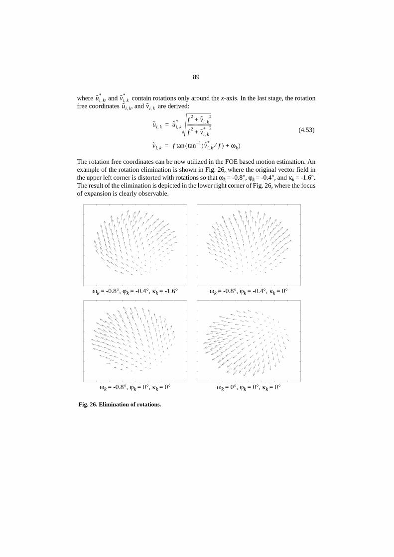
89
where contain rotations only around the x-axis. In the last stage, the rotationfree coordinates are derived:
(4.53)
The rotation free coordinates can be now utilized in the FOE based motion estimation. Anexample of the rotation elimination is shown in Fig. 26, where the original vector field inthe upper left corner is distorted with rotations so that ωk = -0.8°, ϕk = -0.4°, and κk = -1.6°.The result of the elimination is depicted in the lower right corner of Fig. 26, where the focusof expansion is clearly observable.
ui k,* and vi k,
*,ui k, and vi k,,
vi k, f tan 1– vi k,* f⁄( ) ωk+( )tan=
ui k, ui k,* f 2 vi k,
2+
f 2 vi k,* 2
+----------------------=
Fig. 26. Elimination of rotations.
ωk = -0.8°, ϕk = -0.4°, κk = -1.6° ωk = -0.8°, ϕk = -0.4°, κk = 0°
ωk = -0.8°, ϕk = 0°, κk = 0° ωk = 0°, ϕk = 0°, κk = 0°

90
4.6. Linear reconstruction
As the relative position of the camera in the sequence has been determined, the lines of thesight from camera focus to the features can be expressed in a fixed 3-D coordinate system.In principle, the 3-D coordinates of the features are obtained from the intersection of theselines. However, due to the measurement noise, the lines may not cross or there may be sev-eral crossings for a single feature. Hence, we need to estimate the feature location based onseveral observations.
Let us assume that the measurement noise is independent, normally distributed with var-iance σ, and the perturbation in image coordinates caused by motion estimation errors isnegligible with respect to σ. These assumptions demand that the pixels are square and thecamera motion is estimated from several features.
A relationship between the 3-D feature location and corresponding measure-ments at time instants k = 0,..., M can be derived from the camera model of Eq.(4.26) and the measurement model of Eq. (4.32):
(4.54)
As we can see, the problem of computing from noisy observations is nonlinear.However, it can be linearized by multiplying both sides of the equation by and re-arranging the terms so that
(4.55)
or more compactly
The right-hand side of Eq. (4.55) can be minimized in a least squares sense by applying theweighted least squares estimator
(4.56)
where is a 2(M + 1) by 2(M + 1) weighting matrix that has the following structure:
xi yi zi, ,( )Ui k, V i k,,( )
Ui k,
V i k,
fzi tz k,+-----------------
xi tx k,+
yi ty k,+
εi k,
ηi k,
+=
xi yi zi, ,( )zi tz k,+
f 0 Ui 0,–
0 f V i 0,–
..
....
..
.
f 0 Ui M,–
0 f V i M,–
xi
yi
zi
U i 0, tz 0, ftx 0,–
V i 0, tz 0, fty 0,–
..
.
Ui M, tz M, ftx M,–
V i M, tz M, fty M,–
–
ε– i 0, zi tz 0,+( )η– i 0, zi tz 0,+( )
..
.
ε– i M, zi tz M,+( )η– i M, zi tz M,+( )
=
Aipi ci– ei=
pi AiT WiAi( )
1–Ai
T Wici=
Wi

91
(4.57)
In general, computing the estimate is an iterative process. For example, the IRLS pro-cedure given in Section 2.4.4. can be applied. The solution converges typically after a fewiterations, and therefore, it is computationally much lighter than the iterative fitting of Eq.(4.54). However, if the camera motion is almost lateral, i.e. tz, k is approximately constant,the weighting matrix can be replaced with an identity matrix. As a consequence, no itera-tions are required.
4.6.1. CRLB for reconstruction accuracy
In order to test the 3-D reconstruction accuracy of the algorithm the Cramer-Rao lowerbound (CRLB) is derived. Therefore, the probability density function of the measurementvector is required. Under the assumption of Gaussiannoise we obtain
(4.58)
where
The Fisher information matrix can be now expressed as
(4.59)
Wi
zi tz 0,+( ) 2– 0 … 0 0
0 zi tz 0,+( ) 2– … 0 0
..
.... ... ..
....
0 0 … zi tz M,+( ) 2– 0
0 0 … 0 zi tz M,+( ) 2–
=
pi
mi U i 0, V i 0, … Ui M, V i M,,, ,,[ ]T=
p mi ni[ ] 1
2πσ2-----------------
M
1
2σ2--------- mi ni–( )T mi ni–( )–
exp=
ni
f xi tx 0,+( )zi tz 0,+
---------------------------f yi ty 0,+( )
zi tz 0,+--------------------------- …
f xi tx M,+( )zi tz M,+
-----------------------------f yi ty M,+( )
zi tz M,+-----------------------------, , , ,
T
=
Ii1
σ2-----
xi∂∂ni
T
xi∂∂ni
xi∂∂ni
T
yi∂∂ni
xi∂∂ni
T
zi∂∂ni
yi∂∂ni
T
xi∂∂ni
yi∂∂ni
T
yi∂∂ni
yi∂∂ni
T
zi∂∂ni
zi∂∂ni
T
xi∂∂ni
zi∂∂ni
T
yi∂∂ni
zi∂∂ni
T
zi∂∂ni
=

92
Solving the partial derivatives yields
(4.60)
The CRLB is obtained by inverting the matrix Ii:
(4.61)
This bound can be used for evaluating the performance of the 3-D measurement algorithm.As well as in motion estimation, the performance of the least squares estimator of Eq.(4.56) is evaluated by using simulations. The RMS error is acquired by estimating the fea-ture positions from a large number of simulated image sequences. The RMS error is thencompared with the CRLB derived here. Unbiasness of the estimator cannot be assured, be-cause matrices Ai and ci in Eq. (4.56) are statistically depended. The bias is therefore alsodetermined in simulations. The results of the tests are reported in Chapter 5.
4.6.2. Accuracy of the measurement system
In a practical 3-D measurement system, the camera translation is perpendicular to the tar-get. Due to the larger field of view, it is more advantageous to move the camera along thehorizontal image axis than vertical axis. Therefore, we may assume that the y- and z-com-ponents of the camera motion vector are approximately zero and the camera is shifted alongx-axis with equidistant steps ξ. For convenience, let us select the origin of the measurementframe to be located at the halfway of the total camera motion. The translation vector at timeinstant k is then tk = [(k − M/2)ξ, 0, 0]T. This is also illustrated in Fig. 27.
The matrix Ii in Eq. (4.60) can be now simplified to
(4.62)
Iif 2
σ2-----
1
zi tz k,+( )2-------------------------
k 0=
M
∑ 0xi tx k,+
zi tz k,+( )3-------------------------
k 0=
M
∑–
0 1
zi tz k,+( )2-------------------------
k 0=
M
∑ yi ty k,+
zi tz k,+( )3-------------------------
k 0=
M
∑–
xi tx k,+
zi tz k,+( )3-------------------------
k 0=
M
∑–yi ty k,+
zi tz k,+( )3-------------------------
k 0=
M
∑–xi tx k,+( )2 yi ty k,+( )+
2
zi tz k,+( )4----------------------------------------------------------
k 0=
M
∑
=
E pi pi–( ) pi pi–( )T[ ] Ii1–≥
IiM 1+( ) f 2
σ2-------------------------
1
zi2
---- 0xi
zi3
----–
01
zi2
----yi
zi3
----–
xi
zi3
----–yi
zi3
----–12 xi
2 yi2+( ) ξ2M M 2+( )+
12zi4
-----------------------------------------------------------------
=

93
and the inverse of Ii becomes
(4.63)
Due to the aspect ratio 4 : 3 of the most popular video standards (CCIR, RS-170), the fieldof view (FOV) is wider in the horizontal image direction. Thus, by moving the cameraalong the horizontal image axis, we can most efficiently utilize the entire image area. Letus denote the height of the image plane in metric units of length by h. Assuming a squareh by h projection area of the object volume, the apparent motion of the features in the imageplane is limited to h/3, and thus, the total camera motion is limited to
(4.64)
Solving ξ from Eq. (4.64) and replacing it in Eq. (4.63) gives
(4.65)
. .. .. .... .. .... .
..
.
.
tk = [(k − M/2)ξ, 0, 0]T
zx
(xi, yi, zi)
Fig. 27. Camera motion in a practical image sequence based 3-D measurement system.
r
Ii1– 12σ2zi
2
ξ2 f 2M M 1+( ) M 2+( )---------------------------------------------------------
xi2 ξ2M M 2+( )
12------------------------------+ xiyi xizi
xiyi yi2 ξ2M M 2+( )
12------------------------------+ yizi
xizi yizi zi2
=
tx M, tx 0,– Mξhzi
3 f-------= =
Ii1– 108Mσ2
h2 M 1+( ) M 2+( )---------------------------------------------
xi2 h2zi
2 M 2+( )
108Mf 2------------------------------+ xiyi xizi
xiyi yi2 h2zi
2 M 2+( )
108M f 2------------------------------+ yizi
xizi yizi zi2
=

94
It can be noticed that the error in the depth direction does not depend on either the x- or y-coordinates of the feature location. On the other hand, the smallest error in the lateral di-rections is obtained if both xi and yi are zero.
It is quite reasonable to assume that the features are uniformly distributed inside an ob-ject volume whose dimensions are Dx, Dy, and Dz. We may also assume that the expecta-tions E(xi) = 0, E(yi) = 0, and E(zi) = r, where r is the mean distance to the object (see Fig.27). In lateral directions, the dimensions of the object volume are limited by the FOV andthe horizontal camera motion (cf. Eq. (4.64)) so that
(4.66)
The expected values of , , and are then
(4.67)
Assuming that the performance of the estimator in Eq. (4.56) is close to the CRLB, the fol-lowing theoretical values for the average reconstruction error variances in x-, y-, and z-di-rections can be obtained from Eq (4.65):
(4.68)
(4.69)
Absolute accuracy, in terms of metric units, is not always the most relevant way to eval-uate the performance of the measurement system. For example, in laser radar based rangemeasurements it is more meaningful to replace the absolute accuracy with the ratio betweenthe absolute error and the measurement distance, because the absolute accuracy is oftenproportional to the distance between the radar and the target. On the other hand, the mainidea for using camera based 3-D measurement system is to make several observations froma single image. Therefore, the proportion between the 3-D reconstruction error and the prin-cipal dimensions of the object space has been widely used in photogrammetry as a figureof merit. The following notation for the proportional accuracy has been used by Haggrén(1992):
(4.70)
where is the principal dimension of the object volume in metric units of lengthand is the mean standard error of all points in the object volume. Due to the limitedFOV, it is the most appropriate to select . The mean standard error
can be expressed in terms of , , and :
(4.71)
Dx Dyhrf
-----≈=
xi2 yi
2 zi2
E xi2( )
Dx2
12------ h2r2
12 f 2------------ E yi
2( )≈ ≈ and E zi2( )
Dz2
12------ r2+≈=
σx2 σy
2= 9Mσ2r2
M 1+( ) M 2+( ) f 2---------------------------------------------
σ2 Dz2 12r2+( )
12 M 1+( ) f 2-----------------------------------+≈
σz2 9Mσ2 Dz
2 12r2+( )
h2 M 1+( ) M 2+( )---------------------------------------------≈
SσC
σC
D object( )-------------------=
D object( )σC
D object( ) Dx Dy= =σC σx
2 σy2 σz
2
σC
σx2 σy
2 σz2+ +
3------------------------------=

95
The expressions for the average error terms are given in Eqs (4.68) and (4.69). If M is large,these equations can be simplified by using the fact that . The meanstandard error of Eq. (4.71) is approximately
(4.72)
because 1/18 and are very small with respect to and 12. Thus, the expres-sion for the proportional accuracy becomes
(4.73)
where is the principal dimension of the image plane expressed in the same unitsas the standard deviation σ. The square-root term in Eq. (4.73) is denoted by q and is alsocalled the network factor in the photogrammetric literature (e.g. Haggrén 1992). In multi-camera stereo, it primarily depends on the number of the cameras and on the base-to-dis-tance ratio. In a monocular system, it depends on the number of images in the sequence andthe ratio between the vertical image size and the focal length, i.e. the field of view (FOV).The effect of these parameters is visualized in Fig. 28, where the inverse of the proportionalaccuracy 1/ is plotted with three different sequence lengths M = 50, 100, and 150 as afunction of the f/h ratio. The standard deviation of the measurement error has been 0.07 pix-els, and the principal dimension of the image plane 576 pixels.
It can be seen from Fig. 28 that the proportional accuracy of 1/10000 is quite easily at-tained with short focal length optics. For example, a sequence of one hundred images isneeded if the video camera is equipped with a 6.3 mm by 4.7 mm CCD chip and 6 mm op-tics. Naturally, achieving this theoretical accuracy requires that the camera is well calibrat-ed. Especially wide angle optics typically suffer from severe lens distortions. Anotherfactor that may cause the accuracy of the system to deteriorate is the error originating fromthe camera motion estimation process. The influence of that error component is examinedin the experiments in Chapter 5. It should be also noticed that the 3-D accuracy is directlyproportional to the accuracy of the image observations. For example, the standard deviationof 0.07 pixels used in Fig. 28 can be achieved simply by thresholding the image and com-puting the centers of gravity for each feature (Heikkilä & Silvén 1996b). By using morespecialized gray-scale techniques, as discussed in Chapter 2., significant improvement canbe gained in 3-D accuracy.
4.7. Visual tracking
In the previous discussion, the problem of finding the feature correspondences was not han-dled. Automatic matching is generally very problematic, since feature shape may vary sub-stantially between images captured far from each other or from different viewing angles.In addition, if no clues about the mutual camera positions are given, the search for the cor-respondences may be exhaustive. This problem is not so difficult when using image se-quences captured from a moving camera, because the changes in feature locations between
M M 1 M 2+≈+≈
σCσr
f M------------- 6 1
18------ 3 f 2
h2---------+
12Dz
2
r2------+
+σrf
------ 6M----- 1 6 f 2
h2---------+
≈ ≈
Dz2 r2⁄ 3 f 2 h2⁄
SσC
σC
D object( )------------------- σ
h--- 6
M----- 1 6
fh---
2+
=∆σ
D image( )------------------q≈=
D image( )
SσC

96
successive images can be kept small, and if the camera motion is smooth, the feature loca-tions in the forthcoming image can be predicted quite reliably from the former image data.
In the extended Kalman filter (EKF) based motion and the structure estimation used forexample by Silvén and Repo (1993) the correspondence problem is solved by tracking thefeatures image by image. The tracking scheme can be easily augmented to the fusion proc-ess so that the feature locations in the following frame are predicted by projecting the stateestimates and their estimation covariance matrices on the image plane. These projectionsindicate the position and the bounds of the regions where the features are expected to ap-pear. Thus, only a small portion of the image area must be processed in order to find outthe correspondences.
In a 3-D measurement application, the camera motion is more constrained. The cameratransfer mechanism may be designed so that the motion is purely, or at least almost, trans-lational when the effects of small rotations are eliminated with calibration. In addition, thecamera can be shifted with small steps and the distance between successive frames can bekept so short that the disparities in images remain small. A method that properly takes ad-vantage of the known constraints and uses “the closest match” principle may therefore bealready adequate. For obtaining more reliable tracking results, the α-β tracker (Mendel1995, Jezouin & Ayache 1990) can be utilized. The α-β tracker is a linear Kalman filterbased 2-D tracker. Unlike the extended Kalman filter based approach, it does not need any
0.8 1 1.2 1.4 1.6 1.8 2 2.2 2.4 2.62000
4000
6000
8000
10000
12000
14000
16000
18000
Pro
port
iona
l acc
urac
y 1/
S
f/h−ratio
Fig. 28. Approximation of the proportional accuracy based on Eq. (4.73).
M = 50
M = 100
M = 150

97
prior 3-D information of the scene. The basic idea is that the measured image coordinatesare assumed to be independent variables. This assumption makes it possible to separate theimage coordinate space into two independent state variables and with veloc-ities and . The corresponding state equations become
(4.74)
and similarly
(4.75)
where T is the interval between time instants k and k + 1, and are random noisesequences that represent the model perturbation caused by the differences between the lin-ear model and the actual movement of the feature projections. The perturbation is assumedto be white Gaussian noise, although in reality this assumption is not quite correct. How-ever, the performance of the tracker does not typically suffer much from this anomaly.
The corresponding measurement equations are as follows:
(4.76)
and
(4.77)
where and are the measurement noise terms. In this case, composing theKalman filter equations is straightforward. For more information, the reader is referred toMendel (1995) for example. There are also some attractive properties in the filter equationof the α-β tracker: the Kalman gain is scalar that converges rapidly and it can be computedin advance based on the variances of the noise components. These properties make thetracking process computationally less intensive.
4.8. Discussion
There are several ways of extracting 3-D information from image sequences. Batchprocessing is an obvious solution. However, simultaneous estimation of even several hun-dred parameters from a vast amount of data is not practical, especially because the meas-urement model is nonlinear. It is therefore necessary to partition the problem somehow. Ina sequential approach, the observations from a single frame are processed at a time. Theestimates of the current camera motion and 3-D configuration of the features are then up-dated recursively by using an optimal state estimator. The problem in this approach is thecomposition of the optimal filter. The extended Kalman filter (EKF) and the iterated ex-tended Kalman filter (IEKF) techniques are used in the literature, but these techniques havealso some shortcomings. The problem of the initial model is especially evident.
A closed-form solution to the camera motion estimation problem, originally suggested
ui vi,( ) ui viui vi
ui k 1+,
ui k 1+,
1 T
0 1
ui k,
ui k,
T 2 2⁄1
υi k,+=
vi k 1+,
vi k 1+,
1 T
0 1
vi k,
vi k,
T 2 2⁄1
νi k,+=
υi k, νi k,
Ui k 1+, 1 0ui k 1+,
ui k 1+,
εi k 1+,+=
V i k 1+, 1 0vi k 1+,
vi k 1+,
ηi k 1+,+=
εi k 1+, ηi k 1+,

98
by Thompson (1959), has some nice properties, but the accuracy of the estimates obtainedfrom noisy observations is typically quite poor. However, the idea of decomposing motionand structure estimation in separate steps is appealing. If additional constraints on cameramotion are established, the separation can be achieved without reduction in the accuracy.
In this chapter, a technique for determining translational camera motion from image se-quences was presented. A closed-form solution is based on the total least squares estima-tion. Using this motion estimate, a direct technique for determining the 3-D structure canbe applied. Also, methods for evaluating the accuracy of both the motion estimation andthe 3-D reconstruction techniques were given. It was noticed that the accuracy of the meas-urement system is increased mainly by reducing the focal length of the optics, by increasingthe number of the frames in the sequence and by getting more accurate observations fromindividual features. At the end of the chapter, an α-β tracker based approach for determin-ing the correspondences between successive images was presented. However, if the dispar-ity between the images is small and the points are sparsely located, the correspondences canbe determined even with “the closest match” principle.

5. Experiments
5.1. Hardware and test setup
The experimental part of this thesis is subdivided into four sections in which the perform-ance of the data acquisition, camera calibration, motion estimation and structure estimationtechniques are evaluated. This evaluation is based on both simulated and real images. Thevideo camera used in the experiments is an off-the-shelf monochrome CCD camera (SonySSC-M370CE) equipped with a 6.3 mm by 4.7 mm image sensor and a 8.5 mm CosmicarTV lens. The analog CCIR type video signal was digitized with a Sunvideo frame grabber,except in the 3-D measurement tests where Datacube system was used. The correspondingimage sizes were 768 by 576 pixels (Sunvideo), and 512 by 512 pixels (Datacube) with 256gray levels in both cases.
In calibration experiments, as well as in the edge detection and feature extraction tests,a special calibration object was used (see Fig. 18a). The calibration object has three perpen-dicular planar surfaces made of steatite, each face having 256 white circular dots on a blackbackground. The dots (Ø10 mm) form a 16 by 16 square grid (225 mm by 225 mm) with15 mm distance between centers. The object has a matte surface in order to minimize thedisturbing reflections. The overall accuracy of the known dot coordinates is better than 0.1mm and the local accuracy between the dots is about 5 µm. In order to minimize the errorsoriginating from the target, only one surface was used in the edge detection and feature ex-traction experiments. In the camera calibration experiments, two surfaces out of three wereutilized in order to acquire the third dimension, but still cover almost the entire image plane.
In the structure estimation tests, both simulated and real image sequences were used. Inthe case of the real sequences, the test target is a parabolic antenna that has 158 circularpoints on its surface. The diameter of each point is 2.5 cm. The camera was mounted on thewrist of an industrial robot and it was moved almost perpendicularly to the object at a dis-tance of 3 meters with 10 mm steps. The camera motion was stopped each time the imagewas captured in order to avoid motion blur. The total length of the sequence was 57 images,and the features were extracted by using a simple thresholding technique that gives thestandard deviation of the measurement noise about 0.07 pixels (Heikkilä & Silvén 1996b).A sample image from a sequence and the configuration of the system is shown in Fig. 29.

100
The same setup was also used in the simulations. However, due to the non-square pixel sizeof 512 by 512 images, simulated images of 768 by 576 pixels were used. In addition, theeffective focal length of 8 mm was applied instead of 8.5 mm due to its larger field of view.
5.2. Subpixel edge detection and feature extraction
In this section, we compare the performance of different subpixel edge detection and ellipsefitting methods. In edge detection, the moment preserving based technique proposed inSection 2.3.4. is compared with the method suggested by Safaee-Rad et al. (1991). Thecomparison is made by using two real images of the calibration object from two differentangles. In the first view, the angle between the surface normal and the camera principal axiswas small, causing the projections to be nearly circular. In the second view, the angle waslarger and the features were projected as elongated ellipses. The test images are shown inFig. 30.
Fig. 29. Camera view and the configuration of the experimental test system.
x
y
3.0 m
Motion
Camera
Robot
1.8 m z
0.3 m
Fig. 30. Feature pattern from two visual angles.
(a) (b)

101
After subpixel edge detection, the feature positions were located by fitting the quadraticcurve in Eq. (2.11) to the edge data of each feature. Both linear and iterative approacheswith different variations were used. Assuming that the parameter F is normalized to unity,the center point (uc, vc) of the ellipse can be calculated from
(5.1)
Finally, the camera model in Eq. (3.6) was fitted to the observed projection centers in theleast squares fashion by using Levenberg-Marquardt nonlinear regression (Press et al.1992). Since the mutual 3-D locations of the features were known in advance, only the in-ternal and the external camera parameters were needed to be determined. Due to the copla-nar structure of the feature grid, the focal length could not be solved accurately. However,at this stage the only interesting information was the performance of the different edge de-tection and feature extraction methods, and from this point of view, the focal length wasmeaningless. As a figure of merit, the root mean square (RMS) fitting error in image coor-dinates is used.
The results for the images in Fig. 30a and Fig. 30b are represented in Tables 1 and 2,respectively. The RMS fitting error in horizontal (eu) and vertical image (ev) directions aregiven. There are two SMPT based edge detection methods, I and II, applied for both imag-es. Method I proposed by Safaee-Rad et al. (1991) utilizes a circular search region with theradius r = 4.5 pixels. Method II proposed in Section 2.3.4. uses a square 7 by 7 search re-gion, and it assumes the edge curve to be a parabola locally. The features were also locatedwith the grayscale based center of gravity method (CoG). A more profound description ofthe method can be found from Heikkilä & Silvén (1996b).
Four ellipse fitting schemes were applied to the edge data produced by methods I and II.The RMS errors of the direct least squares fitting represented in Section 2.4. with normal-ization F = 1 are given in the second and the third data columns. Also, the other normali-zations (A + C = 1 and A2 + B2 + C2 + D2 + E2 + F2 = 1) were tested, but they did notproduce better results. The next method applied (ILS) uses the nonlinear minimization of
Table 1. The RMS fitting errors for the image shown in Fig. 30a. Edge detection method Iis proposed by Safaee-Rad et al. (1991) and method II is given in Section 2.3.4. Fitting isperformed with direct, iterative (ILS), and iterative reweighted (IRLS) least squaresmethods and with renormalization. As a reference, also results given by the grayscalebased center of gravity method (CoG) are given.
CoGDirect ILS IRLS Renormalization
I II I II I II I II
eu 0.0281 0.0254 0.0237 0.0254 0.0237 0.0254 0.0237 0.0254 0.0237
ev 0.0202 0.0180 0.0179 0.0180 0.0179 0.0180 0.0179 0.0180 0.0179
uc2CD BE–
B2 4AC–------------------------- and vc
2AE BD–
B2 4AC–-------------------------==

102
the perpendicular geometric distances between the model and the edge points observed.The results are given in data columns 4 and 5. The third fitting scheme (IRLS) is the itera-tive reweighted least squares procedure given in Section 2.4.4. and the error function J4 inEq. (2.29) that weights the algebraic distance with the inverse of the gradient. The RMSerrors produced by this method are given in data columns 6 and 7. The last method is renor-malization (Kanatani 1994, Zhang 1995), discussed in Section 2.4.5. The corresponding re-sults are given in the last two data columns.
From Table 1, we can directly see that each ellipse fitting technique tested producedsimilar errors, and only the center of gravity method gave clearly worse results. Based onthis observation, we may state that with circular projections, using iterative fitting methodsinstead of direct methods does not provide any improvement in accuracy. The reason forthis is that the curvature does not alter significantly in different parts of the edge curve. Thisis also the reason for the result that both edge detection methods operated almost uniformly.
The results in Table 2, obtained from the image shown in Fig. 30b, are quite different.As in the previous case, the center of gravity method has the poorest performance. Amongthe fitting techniques, the direct method produced the largest error. By weighting each ob-servation with the inverse of the gradient we reduced the error slightly. However, the bestfitting result was obtained by using renormalization that overcame the iterative leastsquares method by a small margin. It can be also noticed that in this experiment, the newedge detection algorithm which utilizes the moment based parabola fitting gave more ac-curate results than the method proposed by Safaee-Rad et al.
5.3. Camera calibration
In the calibration experiments, two perpendicular planes of the calibration object were vis-ible at the same time. The centers of the circular features were located by using the momentbased edge detection technique described in Section 2.3.4. (method II in Tables 1 and 2)and renormalization fitting (Kanatani 1994, Zhang 1995). The test image is shown in Fig.31.
The calibration object used is not extremely accurate, and the relative 3-D locations of
Table 2. The RMS fitting errors for the image shown in Fig. 30b. The abbreviations usedare explained in the caption of Table 1.
CoGDirect ILS IRLS Renormalization
I II I II I II I II
eu 0.0307 0.0365 0.0318 0.0321 0.0288 0.0341 0.0301 0.0320 0.0287
ev 0.0347 0.0286 0.0280 0.0263 0.0219 0.0268 0.0239 0.0262 0.0217

103
the feature centers are known only to a certain accuracy. Errors in these coordinates set alimit to the calibration accuracy that can be achieved. In the case of Fig. 31, the principaldimension of the object in the horizontal image direction is about 340 mm, and the maxi-mum error in the 3-D coordinates about 0.1 mm. Assuming that the error is normally dis-tributed with standard deviation σo and maximum error of 3σo, we may consider theproportional accuracy of as a rough estimate for the calibration accuracy achiev-able. The average distance to the object is about 550 mm causing the expected standard er-ror in the projected image coordinates to be about 0.06 pixels based on the aboveuncertainties.
Camera calibration was performed with five different methods. The first method is thedirect linear transformation (DLT) based technique proposed by Melen (1994). In the DLTmethod, the lens distortion is neglected and only five intrinsic parameters are estimated: fo-cal length f, principal point (u0, v0), and linear distortion coefficients b1 and b2. The scalefactor su is assumed to be 1. The second method tested is Tsai’s two step procedure (Tsai1987), where a single radial distortion coefficient k1 is included in the model. The locationof the principal point was assumed to be in the center of the image, i.e, in (384, 288) pixels.Estimation of the camera parameters in Tsai’s method is based on the Radial AlignmentConstraint (RAC). In the third calibration method, the same reduced camera model as inTsai’s method was used. However, the parameter estimation was performed using theLevenberg-Marquardt nonlinear regression (Press et al. 1992) for minimizing the error be-tween the model and the observations. The fourth method tested utilizes the Levenberg-Marquardt technique and the full camera model given in Eq. (3.6). The last method includesan additional step that corrects the asymmetric projection error of the ellipse centers (seeSection 3.5.3.). The resulting intrinsic and extrinsic camera parameters with correspondingroot mean square (RMS) errors eu, ev, and averages (bias) bu, bv of the error terms in thehorizontal and vertical image directions are given in Table 3.
If we consider the RMS error of the residual as a figure of merit, we can notice that the
Fig. 31. Calibration image.
1 10000⁄

104
DLT method produced the worst result, and on the other hand the nonlinear optimizationmethods gave clearly the best estimates. This is quite obvious, since the camera models inthe nonlinear optimization cases are more elaborate than in the DLT method. On the otherhand, Tsai’s method seems to suffer from the problem that the principal point location can-not be solved simultaneously, which causes the error to be biased. In this experiment, boththe DLT and Tsai’s method produced unacceptable calibration results. However, the pa-rameter values computed based on these techniques can be used for initializing the nonlin-ear optimization step.
Table 3. Calibration results with two linear (DLT, Tsai’s method), and three nonlinearminimization techniques (reduced and full model, asymmetry corrected observations).
DLTTsai’s
methodReducedmodel
Full modelAsymmetry
corrected
su 1 1.0044 1.0042 1.0036 1.0040
f [mm] 7.7819 8.1290 8.2290 8.2832 8.2763
u0 [pixels] 372.6803 384 367.9790 368.2345 367.9736
v0 [pixels] 274.4949 288 304.0804 306.9297 306.2265
k1 [mm-2] - -1.9646e-03 -2.3553e-03 -3.0637e-03 -3.1082e-03
k2 [mm-4] - - - 4.7747e-05 5.0673e-05
p1 [mm-1] - - - 4.2827e-05 3.0726e-05
p2 [mm-1] - - - -1.6807e-05 -2.0618e-05
x0 [mm] -2.1359 -5.7484 -0.7401 -0.8307 -0.7485
y0 [mm] -90.0466 -94.1305 -99.0382 -99.9459 -99.7174
z0 [mm] 299.9403 313.3135 316.0287 317.5454 317.2201
ω [deg] 18.4827 19.8200 20.7479 20.9595 20.9027
ϕ [deg] -42.6994 -43.1218 -41.9399 -41.8985 -41.8961
κ [deg] -14.5181 -15.4513 -16.0739 -16.2171 -16.1784
bu [pixels] 0 -0.6812 0 0 0
bv [pixels] 0 0.0836 0 0 0
eu [pixels] 0.9676 0.4461 0.1051 0.0516 0.0460
ev [pixels] 0.7061 0.3806 0.0886 0.0443 0.0380

105
Comparing the estimates produced by both linear methods with the estimates given bynonlinear optimization, we may notice that Tsai’s technique succeeds slightly better thanthe DLT method, although there is no big difference in the extrinsic parameters that arevery significant from the standpoint of reaching the global minimum in nonlinear optimi-zation. In addition, Tsai’s technique has been reported to give very poor results with certainconfigurations (e.g. Shih et al. 1995). The DLT method is therefore preferred here for pro-viding the initial parameters.
It can be noticed from the relatively large residual that the reduced camera model usedin Tsai’s method is not adequate, even if nonlinear optimization is applied. Only the fullcamera model with two radial and two tangential distortion coefficients provides the ex-pected accuracy. After asymmetry correction of the ellipse locations, the residual getsslightly smaller. The remaining error indicates even better 3-D accuracy that was expected.
Next, we concentrate on the image correction described in Section 3.4. using the physi-cal camera parameters in the last column of Table 3. First, an equally spaced grid (40 by40) of tie-points was generated that cover the entire image and a small proportion(10%) outside of the effective area so that acceptable results also near the image boundariescould be guaranteed. The corresponding distorted coordinates were calculated us-ing Eqs (3.4) and (3.5) and the parameters of the inverse model a1,..., a8 were estimatedusing Eq. (3.22). The resulting parameters are given in Table 4.
The performance of the inverse model was tested by generating another set of points thatwas first distorted with Eqs (3.4) and (3.5). Correction was then performed with the inversemodel of Eq. (3.20) by using the parameters a1,..., a8 in Table 4. The magnitude of the re-maining error in distortion correction is presented as an error surface with respect to the im-age coordinates u and v in Fig. 32a. The maximum error in this case is clearly less than0.001 pixels. For comparison, also the error surface of Melen’s iterative method (see Eq.(3.18)) is given in Fig. 32b, where the maximum error is over 0.1 pixels.
5.4. Motion estimation
The performance of the focus of expansion (FOE) based motion estimation technique dis-cussed in Section 4.5.2. was compared with the Cramer-Rao lower bound (CRLB) by usingsimulated image sequences. Two motion vectors t1 = [10, 0, 1]T mm and t2 = [10, 0.5,0.01]T mm were used between frames. For both directions, several sequences of M = 56frames were generated in which the number of features N was increased from 10 to 158,and the points were randomly selected. The observations produced were contaminated by
Table 4. Parameters of the inverse model.
a1 (x 10-3) a2 (x 10-4) a3 (x 10-5) a4 (x 10-5) a5 (x 10-4) a6 (x 10-7) a7 (x 10-7) a8 (x 10-2)
-7.6526 1.8996 -3.0780 2.0731 2.4439 -2.0692 3.3337 -1.0759
ui vi,( )
ui' vi',( )

106
white Gaussian noise with the standard deviation of 0.07 pixels. The simulations were per-formed 1000 times and the final results were obtained by averaging individual outcomes inorder to eliminate random variation included in a single realization.
The standard deviation of the minimum error (CRLB), the root mean square (RMS) er-ror of the simulated results, and the average of the error (bias) are plotted in Fig. 33 for eachelementary direction x, y, and z, where the x- and y-axes are collinear with the u- and v-axesof the image plane, respectively, and the z-axis lies along the optical axis. The remainingscale factor was derived by using the true distances M . ||t1|| and M . ||t2|| between the firstand the last camera positions as a reference.
It can be noticed that the error in the z-direction has the largest magnitude. The RMSerror is about 0.5 mm for a small set of features (N = 10), but it is reduced to 0.15 mm whenthe number of features is increased to around 100 points. There are no significant differenc-es in the performance of the estimator between the two translation directions, although inthe second case, the motion is almost lateral causing the FOE to be located very far fromthe principal point. Further examinations have shown that the estimator succeeds equallywell if the motion is completely lateral. It is also observed from Fig. 33 that the estimationerror is close to the CRLB in the y- and z-direction which indicates almost optimal efficien-cy of the TLS based estimation technique. The error in the x-direction is larger than wouldhave been expected based on the CRLB. This difference is explained by an additional errororiginating from scale factor estimation with Eq. (4.50), which treats both x- and y- direc-tions equally causing the remaining error to have the same distribution.
Another criterion of optimality is the unbiasness of the estimator. From Fig. 33 it can beobserved that for each elementary direction x, y, and z, the estimator produces almost zero-bias results in both cases. Small variation in the bias is due to the finite number of simulatedresults that have been used to produce the curve.
In the next experiment, the robustness of the motion estimation technique was tested bymodifying the measurement noise characteristics. The standard deviation of the measure-ment noise was increased from 0.05 to 0.45 pixels, and the resulting error was compared
Fig. 32. The error surface in image correction for (a) the inverse model based method, and (b)the Melen’s method.
(a) (b)
0.002
0.0015
0.001
0.0005
0600
500400
300200
1000 0
200400
600800
u-axis [pixels]v-axis [pixels]
Error [pixels]
Implicit method
0.14
0.12
0.1
0.08
0600
500400
300200
1000 0
200400
600800
u-axis [pixels]v-axis [pixels]
Error [pixels]
Melen’s method
0.06
0.04
0.02

107
Fig. 33. Motion estimation errors (bias, RMSE) and the CRLB for two motion vectors t1 = [10,0, 1]T mm (on the left) and t2 = [10, 0.5, 0.01]T mm (on the right). Errors are given for eachelementary direction x, y, and z (M = 56, f = 8 mm, σ = 0.07 pixels).
0.09 ___= bias_ _ = RMSE..... = CRLB0.08
0.07
0.06
0.05
0.04
0.03
0.02
0.01
0
-0.010 20 40 60 80 100 120 140 160
Error in x-direction (motion/step: [10, 0, 1] mm)Error[mm]
Number of features
0.09 ___= bias_ _ = RMSE..... = CRLB0.08
0.07
0.06
0.05
0.04
0.03
0.02
0.01
0
-0.010 20 40 60 80 100 120 140 160
Error in x-direction (motion/step: [10, 0.5, 0.01] mm)Error[mm]
Number of features
0.09 ___= bias_ _ = RMSE..... = CRLB0.08
0.07
0.06
0.05
0.04
0.03
0.02
0.01
0
-0.010 20 40 60 80 100 120 140 160
Error in y-direction (motion/step: [10, 0, 1] mm)Error[mm]
Number of features
0.09 ___= bias_ _ = RMSE..... = CRLB0.08
0.07
0.06
0.05
0.04
0.03
0.02
0.01
0
-0.010 20 40 60 80 100 120 140 160
Error in y-direction (motion/step: [10, 0.5, 0.01] mm)Error[mm]
Number of features
0.5 ___= bias_ _ = RMSE..... = CRLB
0.4
0.3
0.2
0.1
0
0 20 40 60 80 100 120 140 160
Error in z-direction (motion/step: [10, 0, 1] mm)Error[mm]
Number of features
0.5 ___= bias_ _ = RMSE..... = CRLB
0.4
0.3
0.2
0.1
0
0 20 40 60 80 100 120 140 160
Error in z-direction (motion/step: [10, 0.5, 0.01] mm)Error[mm]
Number of features

108
with the corresponding CRLB. If the error was higher than three times the CRLB, the esti-mator was judged to have failed. The proportion of failures for different numbers of fea-tures (N = 10, 20, 50, and 158) is plotted in Fig. 34a with respect to the standard deviationof the measurement noise. The corresponding CRLB of the z-coordinate is given in Fig.34b. In this case, the results show that the FOE based motion estimation technique workswell when the standard deviation of the measurement noise in observed image coordinatesis less than 0.2 pixels, and even with 0.3 pixels noise, the error rate is less than 12% fordifferent N values. For more extensive noise, the failure rate is rapidly increased. This isquite obvious because the interframe translation was only about 10 mm which caused ap-proximately 3 pixels disparity between images. As the standard deviation of the measure-ment noise becomes large enough, the original information cannot be properlydistinguished from noisy observations. As a result, a breakdown point is achieved. For dif-ferent system configurations and motion lengths, the breakdown point can be elsewhere.
5.5. Structure estimation
The combined motion estimation and 3-D reconstruction algorithm is first compared withthe CRLB. Using the camera motion vector [10, 0, 1]T mm, the performance was measuredwith different sized feature sets (10 - 158). The root mean square error and the correspond-ing CRLB for x-, y- and z-directions are plotted in Fig. 35a. From these results, it can beobserved that the number of features does not significantly affect the total 3-D accuracy.As the number of features decreases to under 40, the RMS error starts to grow slightly, butthis effect is still quite small. In Fig. 35b the corresponding bias of the estimates is plotted.It can be noticed that the systematic error in all coordinate directions is minute. The maxi-
ig. 34. (a) The robustness of the FOE based motion estimation technique. The diagram showshe proportion of failures for the different number of features used (N = 10, 20, 50, and 158)ith respect to the standard deviation of the measurement noise. (b) The correspondingramer-Rao lower bound for the estimate of the z-coordinate (M = 56, f = 8 mm, t = [10, 0, 1]T
m).
N = 158
N = 50
N = 20
N = 10
(a) (b)
N = 158
N = 50
N = 20
N = 10
Proportion of faulty estimates100
90
80
70
60
50
40
30
20
10
00.05 0.1 0.15 0.2 0.25 0.3 0.35 0.4 0.45
Err
or r
ate
[%]
Standard deviation of the measurement noise [pixels]
Cramer-Rao lower bound for z-coordinates4
3.5
3
2.5
2
1.5
1
0.5
00.05 0.1 0.15 0.2 0.25 0.3 0.35 0.4 0.45
Sta
ndar
d de
viat
ion
of th
e es
timat
ion
erro
r [m
m]
Standard deviation of the measurement noise [pixels]

109
mum bias is in the z-direction, which is about 0.03 mm, corresponding a relative error of with respect to the measurement distance.
The image sequences generated are based on pure translational camera motion. Howev-er, in reality the assumption of pure translation may be difficult to achieve. Therefore it isinteresting to know the amount of rotation the motion and structure estimators can tolerate.In Fig. 36a, the camera motion between frames includes also small rotations so that all threeEuler rotation angles (ω, ϕ, κ) are increased gradually. The 3-D reconstruction error in dif-ferent elementary coordinate directions is plotted as a function of the total rotation, i.e., therotation between the first and the last camera positions. The number of the frames in thesequence is 57, and thus the inter-frame rotation is the total rotation divided by 56. It canbe observed that the total rotation of 0.1° in all angles approximately duplicates the recon-struction error. The increase in the error is so significant that it should be eliminated by uti-lizing the procedure described in Section 4.5.5. In Fig. 36b, the rotation parameters arezero-mean equally distributed Gaussian random variables. The reconstruction error is plot-ted with respect to the standard deviation of the inter-frame rotation angles. It can be no-ticed that even when the standard deviation in the angles between the frames is 0.05°, theerror is only slightly increased. As a consequence, small random rotations are not consid-ered to be as harmful as the systematic rotations.
In the next experiment, the performance of other motion and structure estimation meth-ods are compared with the combination of the FOE based technique and the direct 3-D re-construction. The methods tested are the epipolar constraint based linear technique, theextended Kalman filter (EKF), the iterated extended Kalman filter (IEKF) with three iter-ations, and the batch technique with Levenberg-Marquardt optimization.
The recursive and batch methods require initial guesses for the 3-D model structure andthe camera motion. In the cases of EKF and IEKF, the features were assumed to be locatedat intersections of the lines of sight and a plane orthogonal to the principal axis of the cam-era in three meters distance. Gaussian noise components with 1 mm standard deviation
1 100000⁄
Fig. 35. The effect of the feature set size on the 3-D reconstruction accuracy: (a) the CRLB andRMS error, and (b) the average bias in the estimated coordinates (M = 56, f = 8 mm, σ = 0.07pixels, t = [10, 0, 1]T mm).
CRLB for z-coordinate
RMSE for z-coordinate
RMSE for x-coordinateRMSE for y-coordinate
CRLB for x-coordinateCRLB for y-coordinate
Bias for x-coordinate
Bias for y-coordinate
Bias for z-coordinate
(a) (b)
0.6
0.5
0.4
0.3
0.2
0.1
020 40 60 80 100 120 140
Number of features
Err
or [m
m]
The RMSE and CRLB for 3-D reconstruction
20 40 60 80 100 120 140Number of features
Err
or [m
m]
The bias for 3-D reconstruction0.04
0.03
0.02
0.01
0
-0.01
-0.02
-0.03
-0.04

110
were added to the true camera motion vector t = [30, 0, 3]T mm and the result was used asa starting value for sequential motion estimation. Only translational components of the mo-tion were estimated and the rotations were omitted. For the batch technique, the true motionvectors were first contaminated by Gaussian noise with 1 mm standard deviation and thenused as initial values for the iterative least squares estimation. In this experiment, thenumber of frames in a sequence was limited to 20, because the batch technique could nothandle more measurements in reasonable time. The number of the features per frame was158 for all sequences.
The average errors based on 200 simulated sequences are shown in Table 5. The firstthree rows of the table represent the RMS errors in x-, y-, and z-directions, and the last rowshows the corresponding proportional accuracy with respect to the principal dimension ofthe target (1.8 m). As a reference, theoretical error limits based on the CRLB are given inthe last column of the table. It can be immediately noticed that the epipolar constraint basedtechnique produced much worse results than the other techniques. The obvious reason isthat translation cannot be reliably discriminated from rotation without knowing the struc-ture in advance. The FOE based technique and the batch technique gave an accuracy thatis almost optimal, but in practice, also the EKF and IEKF techniques succeeded almostcomparably. Thus, the greatest advantage of the FOE based method is the computationalspeed. Its Matlab implementation was about 40 times faster than the corresponding IEKFimplementation. The batch method was approximately as slow as the IEKF, but for longersequences its computational cost would be higher. The corresponding approximation of thetheoretical accuracy obtained from Eq. (4.73) gives the proportion of 1/3500, which is veryclose to the actual results.
Fig. 36. The effect of small camera rotations on the 3-D reconstruction accuracy: (a) system-atic rotations in all angles, and (b) random rotations in all angles (N = 158, M = 56, f = 8 mm,σ = 0.07 pixels, t = [10, 0, 1]T mm).
(a) (b)
1.2
1
0.8
0.6
0.4
0.2
00.01 0.02 0.03 0.04 0.05 0.06 0.07 0.08 0.09 0.1
The effect of systematic rotations on the 3-D estimation error
_ _ = x-, y-coord.___ = z-coord.
Rotation [degrees]
Err
or [m
m]
1.2
1
0.8
0.6
0.4
0.2
00.01 0.02 0.03 0.04 0.05 0.06 0.07 0.08 0.09 0.1
The effect of random rotations on the 3-D estimation error
_ _ = x-, y-coord.___ = z-coord.
Rotation [degrees]
Err
or [m
m]

111
In the last simulation, the 3-D reconstruction accuracy of the EKF, IEKF, and FOEbased methods were compared by increasing the number of the images in the sequence. Thetotal camera travel remained the same in all the sequences, but the distance between theframes was decreased. Within the sequences, equidistant intervals were used. The shortestsequence was 20 frames and the longest 150 frames, and all the sequences included 158features. The proportional accuracies of the methods are plotted in Fig. 37, where we canimmediately notice that the FOE based technique gave the best accuracy, but both the EKFand IEKF techniques succeeded almost as well. At least in this case, iterating does not pro-vide much increase in the accuracy of the Extended Kalman filter. The theoretical accuracyplotted in Fig. 37 is based on Eq. (4.73), and therefore, it is an approximation. This explainsthe difference between the theoretical and the actual curves. With long sequences, Eq.(4.73) gave a slightly too optimistic estimate of the attainable proportional accuracy.
Table 5. 3-D reconstruction error and the proportional accuracy for five differentestimators with the corresponding theoretical limits (N = 158, M = 20, f = 8, σ = 0.07pixels, t = [30, 0, 3]T mm).
Epipolar EKF IEKF Batch FOE Theoretical
RMSEx [mm] 1.0466 0.2077 0.1564 0.1408 0.1407 0.1384
RMSEy [mm] 1.0417 0.1977 0.1460 0.1310 0.1310 0.1308
RMSEz [mm] 0.9146 0.8909 0.8903 0.8481 0.8481 0.8474
Prop. accuracy 1/1795 1/3331 1/3405 1/3585 1/3585 1/3589
20 40 60 80 100 120 140 1600
1000
2000
3000
4000
5000
6000
7000
8000
9000
10000
...... = theoretical_ _ = FOE._._ = EKF___ = IEKF
Number of images
Pro
port
iona
l acc
urac
y 1/
S
Fig. 37. The proportional 3-D reconstruction accuracy for various sequence lengths with dif-ferent estimation techniques (N = 158, f = 8, σ = 0.07 pixels).

112
The 3-D measurement technique was also tested with real image sequences. However,determining the absolute accuracy was found to be an extremely difficult task, becauseeven more accurate reference measurements were required. The reference coordinates pro-vided by a laser coordinate meter were not accurate enough to enable a reliable comparison,cf. Heikkilä & Silvén (1996a). Repeatability was therefore considered to be a better meas-ure of accuracy. In repeatability tests, the measurement procedure was repeated twice andthe 3-D reconstruction results were then compared. This comparison does not completelyreveal the systematic errors caused by, for example, faulty camera calibration, but it is morea feasibility test which shows the performance of the image sequence based measurementtechnique in practice.
The setup of the experimental system is described in Section 5.1. Due to the 8.5 mm op-tics and shorter imaging distance, not all of the 158 features fitted in the image at the sametime (see Fig. 29). A subset of only 102 features was therefore used, and the correspondingprincipal dimension of the object space was about 1.6 m. Due to the non-squarepixel size (6.3 mm by 4.7 mm image area was digitized to 512 by 512 pixels), the meanstandard error of the measurement noise in the image plane becomes approximately
µm. Thus, the theoretical proportional accuracy fromEq. (4.73) for a sequence of 57 frames (M = 56) becomes about 1/4200.
Two sequences a and b were captured, and the motion estimation process for both se-quences was performed with the FOE based method (Section 4.5.2.), and the 3-D coordi-nates (xa, ya, za) and (xb, yb, zb) were estimated by using the direct reconstruction technique(Section 4.6.). These results were evaluated by first calculating the differences
, , and that are random vectors with zero meanand variances , , and . Now, the mean standard error can be estimatedbased on Eq. (4.71):
(5.2)
The proportional accuracy is calculated from Eq. (4.70). The results are given in thefirst row of Table 6. For comparison, the results produced by the EKF method are also giv-en, so that in the second row, only the translational components of the motion were estimat-ed, and in the third row, camera rotation estimation was also utilized. As it can be seen,estimation of rotations did not improve the results. On the contrary, the accuracy wasslightly reduced. Again, the FOE based method produced the highest accuracy, which isalso quite close to the theoretical value 1/4200.
Table 6. The results of the repeatability test for real image sequences.
[mm2] [mm2] [mm2] [mm]
FOE 2.8618 1.9960 101.5034 0.4169 1/3838
EKF (3 dof) 3.1417 1.8726 103.8177 0.4217 1/3794
EKF (6 dof) 3.0877 2.1647 104.8581 0.4242 1/3772
D object( )
σ 0.07= 512⁄ 6.3 4.7+( ) 2⁄⋅ 0.75≈
dx xb xa–= dy yb ya–= dz zb za–=2σx
2 2σy2 2σz
2 σC
σC
σx2 σy
2 σz2+ +
3------------------------------
dxT dx dy
T dy dzT dz+ +
6N------------------------------------------------≈=
SσC
dxT dx dy
T dy dzT dz
σC SσC

6. Conclusions
Multi-camera stereo vision has been traditionally utilized for obtaining 3-D informationfrom optical data. Recently, monocular vision with a moving camera has also turn out to bea technique worth of consideration for 3-D modeling problems. The procedure for obtain-ing accurate 3-D information from intensity image sequences requires several imageprocessing and parameter estimation steps. In this study, the objective was to develop thosetechniques that make the single camera approach a realistic choice for measurement appli-cations.
The first problem considered was accurate data acquisition from intensity images. It wasassumed that the objects to be measured consist of some visible features. These features areeither natural or artificial patterns. In this thesis, only lines and circles were considered dueto their simple geometrical models and their commonness in man-made scenes. The fea-tures observed are parametrized in a sequence of different steps. First, it is necessary to de-termine the feature locations with coarse precision in order to focus the subsequent imageprocessing stages into small regions of interest. This stage is called labelling. The refiningstage is needed for locating the boundary curves of the feature projections, initially in a lessaccurate manner, and after that with subpixel precision. A novel technique based on a sam-ple-moment-preserving principle and parabolic curve fitting was introduced for subpixeldetection of curved feature boundaries.
In the extracting stage, the parameters characteristic to the feature type are estimatedfrom the edge data. For this purpose, several estimation methods were discussed. For linefeatures, there is a closed-form solution available that minimizes the perpendicular errorbetween the observations and the line. In the case of curved features, the parameter estima-tion step is not as straightforward. There are both direct and iterative methods available.The estimates obtained by using direct methods are high curvature biased. They are com-putationally several times faster than iterative methods, but they tend to produce worse es-timates. The difference in performance is clear, especially, when the circular features areobserved from inclined angles. Therefore, it depends on the application and the resourcesavailable which approach should be used. The experiments performed showed that a com-bination of the new subpixel edge detector and the fitting technique called renormalizationproduced the best measurement accuracy among other tested methods.
Geometric camera calibration is needed for correcting the spatial errors in the images.

114
Without proper calibration the 3-D estimates would become inaccurate. A great deal of at-tention has been paid to calibration issues for a long time. Especially in computer visionliterature many camera calibration procedures have been suggested. However, most ofthem are based on simplified camera models, and they are not suitable as such for accuratemeasurements. It was noticed that the classical calibration method mainly used in the fieldof photogrammetry is the only method that can achieve adequate precision. The numericalstability and the convergence speed of the classical method can be improved by selectingthe starting point of the iteration carefully. For example, direct linear transformation (DLT)can be applied for obtaining the initial guess.
There are several error sources that may affect the accuracy of the estimated camera pa-rameters. Some of the errors are caused by an insufficient camera model and others are dueto some external factors. These error sources were discussed in the context of camera cali-bration. In this thesis, an additional step for the conventional calibration procedure is sug-gested that compensates for the error caused by the asymmetric projection of the circularfeatures. A new approach for correcting the image coordinates was also introduced. Thecorrection is based on a simple inverse distortion model, whose parameters can be easilycomputed from the physical camera parameters.
Integrating 2-D coordinate data from individual images to a non-redundant 3-D modelwas handled in the third part of this thesis. The problem in the integration process is theamount of data, and on the other hand, the large number of estimated parameters. For eachcamera position and angle there are generally six parameters that must be estimated in orderto determine the relative positions of the features. A batch technique is therefore not prac-tical for solving the problem. The Kalman filter based sequential approaches (EKF, IEKF)are competent solutions, especially for long sequences. In the case of short sequences, thelack of an adequate initial model can cause inaccuracy.
Making accurate 3-D measurements does not necessarily require rotating the camera. Ifthe camera motion is purely translational, or the rotations are known in advance, a closed-form solution can be found for estimating the three remaining motion parameters. The so-lution presented in this thesis utilizes the focus of expansion (FOE), which is located byapplying the total least squares estimation technique. Using the motion parameters obtainedalso a direct solution to the 3-D structure estimation problem is possible. This approach wasfound to be much faster than the nonlinear techniques.
The accuracy considerations and the experiments performed showed that the image se-quence based approach is a potential technique for performing accurate coordinate andshape measurements. It can achieve a proportional accuracy of even by properlyselecting the focal length and the number of the images in the sequence. Using the directsolution in the motion estimation problem enables a reasonably fast approach for demand-ing measurement applications. However, implementing the complete measurement systemis left as subject of future work.
1 10000⁄

References
Abdel-Aziz YI & Karara HM (1971) Direct linear transformation into object space coordinates inclose-range photogrammetry. Proc. Symposium on Close-Range Photogrammetry, Urbana,Illinois, 1-18.
Ballard DH (1981) Generalizing the Hough transform to detect arbitrary shapes. Pattern Recognition13: 111-122.
Ballard DH & Kimball OA (1983) Rigid body motion from depth and optical flow. Computer Vision,Graphics, and Image Processing 22(1): 95-115.
Batista J, Dias J, Araujo H & de Almeida A (1993) Monoplane Camera Calibration - Iterative Multi-Step Approach. Proc. 4th British Machine Vision Conference, Guildford, England, 479-488.
Beardsley P, Murray D & Zisserman A (1992) Camera calibration using multiple images. Proc. 2ndEuropean Conference on Computer Vision, Santa Margherita Ligure, Italy, 312-320.
Besl PJ (1988) Active, optical range imaging sensors. Machine Vision and Applications 1(2): 127-152.
Beyer HA (1990) Linejitter and geometric calibration of CCD cameras. ISPRS Journal ofPhotogrammetry and Remote Sensing 45: 17-32.
Bookstein FL (1979) Fitting conic sections to scattered data. Computer Graphics and ImageProcessing 9: 56-71.
Bopp H & Krauss H (1978) An orientation and calibration method for non-topographic applications.Photogrammetric Engineering and Remote Sensing 44(9): 1191-1196.
Broida T & Chellappa R (1986) Estimation of object motion parameters from noisy images. IEEETransactions on Pattern Analysis and Machine Intelligence 8(1): 90-99.
Broida T & Chellappa R (1989) Performance bounds for estimating three-dimensional motionparameters from a sequence of noisy images. Journal of Optical Society of America A6: 879-889.
Brown DC (1966) Decentering distortion of lenses. Photogrammetric Engineering 32: 444-462.Brown DC (1971) Close-range camera calibration. Photogrammetric Engineering 37: 855-866.Bruss AR & Horn BKP (1983) Passive navigation. Computer Vision, Graphics, and Image
Processing 21(1): 3-20.Buurman J (1992) Ellipse based stereo vision. Proc. 2nd European Conference on Computer Vision,
Santa Margherita Ligure, Italy, 363-372.Caprile B & Torre V (1990) Using vanishing points for camera calibration. International Journal of
Computer Vision 4: 127-140.Chaudhuri S & Chatterjee S (1991) Performance analysis of total least squares methods in three-
dimensional motion estimation. IEEE Transactions on Robotics and Automation 7(5): 707-714.Chen LH & Tsai WH (1988a) Moment-preserving line detection. Pattern Recognition 21(1): 45-53.

116
Chen LH & Tsai WH (1988b) Moment-preserving curve detection. IEEE Transactions on Systems,Man, and Cybernetics 18(1): 148-158.
Chiorboli G & Vecchi GP (1993) Comments on “Design of fiducials for accurate registration usingmachine vision”. IEEE Transactions on Pattern Analysis and Machine Intelligence 15(12): 1330-1332.
Chou CH & Chen YC (1990) Moment-preserving pattern matching. Pattern Recognition 23(5): 461-474.
Crimmins TR & Brown WR (1985) Image algebra and automatic shape recognition. IEEETransactions on Aerospace and Electronic Systems AES-21: 60-69.
Cui N, Weng J & Cohen P (1994) Recursive-batch estimation of motion and structure frommonocular image sequences. CVGIP: Image Understanding 59(2): 154-170.
Cui Y, Weng J & Reynolds H (1996) Estimation of ellipse parameters using optimal minimumvariance estimator. Pattern Recognition Letters 17: 309-316.
Dickmanns ED & Graefe V (1988) Dynamic Monocular Machine Vision. Machine Vision andApplications 1: 223-240.
Draper N & Smith H (1981) Applied Regression Analysis. 2nd ed., Wiley, New York.Echigo T (1990) A camera calibration technique using three sets of parallel lines. Machine Vision
and Applications 3: 159-167.Faig W (1975) Calibration of close-range photogrammetric systems: Mathematical formulation.
Photogrammetric Engineering and Remote Sensing 41(12): 1479-1486.Faugeras OD, Luong QT & Maybank SJ (1992) Camera self-calibration: theory and experiments.
Proc. 2nd European Conference on Computer Vision, Santa Margherita Ligure, Italy, 321-334.Faugeras OD, Lustman F & Toscani G (1987) Motion and structure from motion from point and line
matches. Proc. 1st International Conference on Computer Vision, London, England, 25-34.Faugeras OD & Toscani G (1986) The calibration problem for stereo. Proc. IEEE Conference on
Computer Vision and Pattern Recognition, Miami Beach, FL, 15-20.Faugeras OD & Toscani G (1987) Camera calibration for 3D computer vision. Proc. International
Workshop on Industrial Applications of Machine Vision and Machine Intelligence, Silken, Japan,240-247.
Ferri M, Mangili F & Viano G (1993) Projective pose estimation of linear and quadratic primitivesin monocular computer vision. CVGIP: Image Understanding 58(1): 66-84.
Ganapathy S (1984) Decomposition of transformation matrices for robot vision. Pattern RecognitionLetters 2: 401-412.
Gelb A (1974) Applied Optimal Estimation. MIT Press, Cambridge, Massachusetts.Golub GH & Van Loan CF (1989) Matrix computations. Johns Hopkins University Press, Baltimore.Grosky WI & Tamburino LA (1990) A unified approach to the linear camera calibration problem.
IEEE Transactions on Pattern Analysis and Machine Intelligence 12(7): 663-671.Gårding J & Lindeberg T (1994) Direct estimation of local surface shape in a fixating binocular vision
system. Proc. 3rd European Conference on Computer Vision, Stockholm, Sweden, 1: 365-376.Haggrén H (1989) Photogrammetric machine vision. Optics and Lasers in Engineering 10: 256-286.Haggrén H (1992) On System Development of Photogrammetric Stations for On-Line Manufacturing
Control. Helsinki University of Technology, Civil Engineering and Building Construction Series97: 9-15.
Haggrén H & Heikkilä J (1989) Calibration of close-range photogrammetric stations using a freenetwork bundle adjustment. The Photogrammetric Journal of Finland 11(2): 21-31.
Hampel F, Ronchetti E, Rousseeuw P & Stahel W (1986) Robust statistics: the approach based oninfluence functions. Wiley, New York.
Han MH & Rhee S (1992) Camera calibration for three-dimensional measurement. PatternRecognition 25(2): 155-164.

117
Haralick RM (1984) Digital step edges from zero crossing of second directional derivatives. IEEETransactions on Pattern Analysis and Machine Intelligence 6: 58-68.
Haralick RM (1989) Determining camera parameters from the perspective projection of a rectangle.Pattern Recognition 22: 223-230.
Haralick RM, Chu YH, Watson LT & Shapiro LG (1984) Matching wire frame objects from their twodimensional perspective projections. Pattern Recognition 17(6): 607-619.
Haralick RM & Joo H (1988) 2D-3D pose estimation. Proc. 9th International Conference on PatternRecognition, Rome, Italy, 385-391.
Haralick RM & Shapiro LG (1992) Computer and robot vision. Addison-Wesley, Reading,Massachusetts.
Hartley RI (1992) Estimation of relative camera positions for uncalibrated cameras. Proc. 2ndEuropean Conference on Computer Vision, Santa Margherita Ligure, Italy, 579-587.
Heeger DJ & Jepson AD (1992) Subspace methods for recovering rigid motion I: algorithm andimplementation. International Journal of Computer Vision 7(2): 95-117.
Heikkilä J & Silvén O (1995) System considerations for feature tracker based 3-D measurements.Proc. 9th Scandinavian Conference on Image Analysis, Uppsala, Sweden, 255-262.
Heikkilä J & Silvén O (1996a) Accurate 3-D measurement using a single video camera. InternationalJournal of Pattern Recognition and Artificial Intelligence 10(2): 139-149.
Heikkilä J & Silvén O (1996b) Calibration procedure for short focal length off-the-shelf CCDcameras. Proc. 13th International Conference on Pattern Recognition, Vienna, Austria, 1: 166-170.
Heikkilä J & Silvén O (1997) A four-step camera calibration procedure with implicit imagecorrection. Proc. IEEE Conference on Computer Vision and Pattern Recognition, San Juan, PuertoRico, 1106-1112.
Ho CT & Chen LH (1995) A fast ellipse/circle detector using geometric symmetry. PatternRecognition 28(1): 117-124.
Horaud R, ConioB, Leboulleux O & Lacolle B (1989) An analytic solution for the perspective 4-pointproblem. Computer Vision, Graphics, and Image Processing 47(1): 33-44.
Horaud R, Dornaika F, Boufama B & Mohr R (1994) Self calibration of a stereo head mounted ontoa robot arm. Proc. 3rd European Conference on Computer Vision, Stockholm, Sweden, 1: 455-462.
Horn BKP & Schunck BG (1981) Determining optical flow. Artificial Intelligence 17: 185-203.Hough PVC (1962) A method and means for recognizing complex patterns. US patent 3.069.654.Huang TS & Faugeras OD (1989) Some properties of the e-matrix in two-view motion estimation.
IEEE Transactions on Pattern Analysis and Machine Intelligence 11: 1310-1312.Huang TS & Netravali AN (1994) Motion and structure from feature correspond-ences: A review.
Proceedings of the IEEE 82(2): 252-268.Huber PJ (1981) Robust statistics. Wiley, New York.Hueckel MF (1971) An operator which locates edges in digitized pictures. Journal of the Association
for Computing Machinery 18: 113-125.Huertas A & Medioni G (1986) Detection of intensity changes with subpixel accuracy using
Laplacian-Gaussian masks. IEEE Transactions on Pattern Analysis and Machine Intelligence8(5): 651-664.
Hummel RA (1979) Feature detection using basis functions. Computer Graphics and ImageProcessing 9: 40-55.
Hung YP & Shih SW (1990) When should we consider lens distortion in camera calibration. Proc.IAPR Workshop on Machine Vision Applications, Tokyo, 367-370.
Hådem I (1981) Bundle adjustment in industrial photogrammetry. Photogrammetria 37(2): 45-60.Illingworth J & Kittler J (1987) The adaptive Hough transform. IEEE Transactions on Pattern
Analysis and Machine Intelligence 9(5): 690-698.

118
Illingworth J & Kittler J (1988) A survey of the Hough transform. Computer Vision, Graphics, andImage Processing 44: 87-116.
Isaguirre A, Pu P & Summers J (1985) A new developement in camera calibration: calibrating a pairof mobile cameras. Proc. International Comference on Robotics and Automation, St. Louis,Missouri, 74-79.
Jain R (1983) Direct computation of the focus of expansion. IEEE Transactions on Pattern Analysisand Machine Intelligence 5(1): 58-64.
Jezouin JL & Ayache N (1990) 3D structure from a monocular sequence of images. Proc. 3rdInternational Conference on Computer Vision, Osaka, Japan, 441-445.
Kabuka MR & Arenas AE (1987) Position verification of a mobile robot using standard pattern. IEEEJournal of Robotics and Automation RA-3(6): 505-516.
Kalman RE (1960) A new approach to linear filtering and prediction problems. Trans. ASME J. BasicEng. Series D 82: 35-46.
Kamgar-Parsi B, Kamgar-Parsi B & Netanyahu NS (1989) A nonparametric method for fitting astraight line to a noisy image. IEEE Transactions on Pattern Analysis and Machine Intelligence11(9): 998-1001.
Kanatani K (1993) Unbiased estimation and statistical analysis of 3-D rigid motion from two views.IEEE Transactions on Pattern Analysis and Machine Intelligence 15(1): 37-50.
Kanatani K (1994) Statistical bias of conic fitting and renormalization. IEEE Transactions on PatternAnalysis and Machine Intelligence 16(3): 320-326.
Karara HM (1989) Handbook of Non-Topographic Photogrammetry. 2nd ed., American Society ofPhotogrammetry, Falls Church, Virginia.
Kay SM (1993) Fundamentals of statistical signal processing. Prentice Hall, Englewood Cliffs, NewJersey.
Kirsch R (1971) Computer determination of the constitutient structure of biologic image. ComputerBiomedical Research 4: 315-328.
Kisworo M, Venkatesh S & West G (1994) Modeling edges at subpixel accuracy using the localenergy approach. IEEE Transactions on Pattern Analysis and Machine Intelligence 16(4): 405-410.
Koivunen V (1993) Processing and Interpretation of 3-D Sensory Data with an Application inGeometric Modeling. Acta Univ Oul C 74: 29-43.
Lee R, Lu PC & Tsai WH (1990) Moment preserving detection of elliptical shapes in gray-scaleimages. Pattern Recognition Letters 11: 405-414.
Lenz RK & Tsai RY (1988) Techniques for calibration of the scale factor and image center for highaccuracy 3-D machine vision metrology. IEEE Transactions on Pattern Analysis and MachineIntelligence 10(5): 713-720.
Li M (1994) Camera calibration of a head-eye system for active vision. Proc. 3rd EuropeanConference on Computer Vision, Stockholm, Sweden, 1: 543-554.
Linnainmaa S, Harwood D & Davis LS (1988) Pose determination of a 3-D object using trianglepairs. IEEE Transactions on Pattern Analysis and Machine Intelligence 10(5): 634-647.
Liu ST & Tsai WH (1989) Moment-preserving clustering. Pattern Recognition 22(4): 433-447.Liu ST & Tsai WH (1990) Moment-preserving corner detection. Pattern Recognition 23(5): 441-460.Liu Y, Huang TS & Faugeras OD (1988) Determination of camera location from 2D to 3D line and
point correspondences. Proc. IEEE Conference on Computer Vision and Pattern Recognition, AnnArbor, MI, 82-88.
Longuet-Higgins HC (1981) A computer algorithm for reconstructing a scene from two projections.Nature 293: 133-135.
Luong QT & Faugeras OD (1994) An optimization framework for efficient self-calibration andmotion determination. Proc. 12th International Conference on Pattern Recognition, Jerusalem,Israel, 248-252.

119
Lyvers EP, Mitchell OR, Akey ML & Reeves AP (1989) Subpixel measurement using a moment-based edge operator. IEEE Transactions on Pattern Analysis and Machine Intelligence 11(12):1293-1309.
Magee MJ & Aggarwal JK (1984) Determining the position of a robot using a single calibrationobject. Proc. IEEE International Conference on Robotics and Automation, Atlanta, GA, 140-149.
Martins HA, Birk JR & Kelley RB (1981) Camera models based on data from two calibration planes.Computer Graphics and Image Processing 17:173-180.
Matthies L, Szeliski R & Kanade T (1988) Kalman filter based algorithm for estimating depth fromimage sequences. Proc. IEEE Conference on Computer Vision and Pattern Recognition, AnnArbor, MI, 199-213.
Melen T (1994) Geometrical modelling and calibration of video cameras for underwater navigation.Dr. ing thesis, Norges tekniske høgskole, Institutt for teknisk kybernetikk.
Mendel JM (1995) Lessons in Estimation Theory for Signal Processing, Communications andControl. Prentice Hall, Englewood Cliffs, New Jersey.
Moring I (1995) Laser radar-based range imaging with applications in shape measurement andmachine control. VTT publications 220: 17-39.
Nadler M & Smith EP (1993) Pattern recognition engineering. Wiley, New York.Nalwa VS & Binford TO (1986) On detecting edges. IEEE Transactions on Pattern Analysis and
Machine Intelligence 8(6): 699-714.O’Gorman F (1978) Edge detection using Walsh functions. Artificial Intelligence 10: 215-223.Penna MA (1991a) Camera calibration: a quick and easy way to determine the scale factor. IEEE
Transactions on Pattern Analysis and Machine Intelligence 13: 1240-1245.Penna MA (1991b) Determining camera parameters from the perspective projection of a
quadrilateral. Pattern Recognition 24: 533-541.Petkovic D, Niblack W & Flickner M (1988) Projection-based high accuracy measurement of straight
line edges. Machine Vision and Applications 1: 183-199.Porrill J (1990) Fitting ellipses and predicting confidence envelopes using a bias corrected Kalman
filter. Image and Vision Computing 8(1): 37-41.Prazdny K (1981) Determining the instantaneous direction of motion from optical flow generated by
a curvilinear moving observer. Computer Vision, Graphics, and Image Processing 17: 238-248.Press WH, Teukolsky SA, Vetterling WT & Flannery BP (1992) Numerical Recipes in C - The Art
of Scientific Computing. 2nd ed., Cambridge University Press.Prewitt J (1970) Object enhancement and extraction. In: Lipkin, B. & Rosenfeld, A. (eds) Picture
Processing and Psychopictorics. Academic Press, New York, p 75-149.Roberts LG (1965) Machine perception of three-dimensional solids. In: Tippet, et al. (eds) Optical
and Electro-optical Information Processing. MIT Press, Cambridge, Massachusetts, p 159-197.Rosin PL (1993) A note on the least squares fitting of ellipses. Pattern Recognition Letters 14(10):
799-808.Röning J, Heikkilä J, Silvén O & Repo T (1994) Laboratory pilot for vision guided palletizing. Proc.
International Conference on Machine Automation: Mechatronics Spells Profitability, Tampere,Finland, 203-213.
Safaee-Rad R, Smith KC & Benhabib B (1990) Accurate estimation of elliptical shape parametersfrom a grey-level image. Proc. 10th International Conference on Pattern Recognition, AtlanticCity, NJ, 20-26.
Safaee-Rad R, Tchoukanov I, Benhabib B & Smith KC (1991) Accurate parameter estimation ofquadratic curves from grey-level images. CVGIP: Image Understanding 54(2): 259-274.
Safaee-Rad R, Tchoukanov I, Smith KC & Benhabib B (1992) Three-dimensional locationestimation of circular features for machine vision. IEEE Transactions on Robotics andAutomation RA-8(5): 624-640.

120
Sampson PD (1982) Fitting conic sections to ‘very scattered’ data: an iterative refinement of thebookstein algorithm. Computer Vision, Graphics, and Image Processing 18: 97-108.
Schwidefsky K & Ackermann F (1976) Photogrammetrie: Grundlagen, Verfahren, Anwendungen.Teubner, Stuttgart.
Serra J (1982) Image Analysis and Mathematical Morphology, Academic Press, New York.Shih TY & Faig W (1987) Physical interpretation of the extended DLT-model. Proc. ASPRS Fall
Convention, American Society for Photogrammetry and Remote Sensing, Reno, Nevada, 385-394.
Shih SW, Hung YP & Lin WS (1993) Accurate linear technique for camera calibration consideringlens distortion by solving an eigenvalue problem. Optical Engineering 32(1): 138-149.
Shih SW, Hung YP & Lin WS (1995) When should we consider lens distortion in camera calibration.Pattern Recognition 28(3): 447-461.
Silvén O & Repo T (1993) Experiments with monocular visual tracking and environment modeling.Proc. 4th International Conference on Computer Vision, Berlin, Germany, 84-92.
Slama CC (ed.) (1980) Manual of Photogrammetry. 4th ed., American Society of Photogrammetry,Falls Church, Virginia.
Smith FG & Thomson JH (1988) Optics. 2nd ed., Wiley, Chichester.Spetsakis ME & Aloimonos Y (1992) Optimal visual motion estimation: A note. IEEE Transactions
on Pattern Analysis and Machine Intelligence 14(9): 959-964.Strang G (1988) Linear algebra and its applications. 3rd ed., Harcourt Brace Jovanovich, San Diego,
California.Strat TM (1984) Recovering the camera parameters from a transformation matrix. Proc. Image
Understanding Workshop, New Orleans, Louisiana, 264-271.Sundareswaran V (1992) A fast method to estimate sensor translation. Proc. 2nd European
Conference on Computer Vision, Santa Margherita Ligure, Italy, 253-257.Tabatabai AJ & Mitchell OR (1984) Edge location to subpixel values in digital imagery. IEEE
Transactions on Pattern Analysis and Machine Intelligence 6(2): 188-201.Tabbone S & Ziou D (1992) Subpixel positioning of edges for first and second order operators. Proc.
11th International Conference on Pattern Recognition, The Hague, Netherlands, 655-658.Thompson EH (1959) A rational algebraic formulation of the problem of relative orientation.
Photogrammetric Record 3(14): 152-159.Thompson EH (1968) The projective theory of relative orientation. Photogrammetria 23(1): 67-75.Tsai RY (1987) A versatile camera calibration technique for high-accuracy 3D machine vision
metrology using off-the-shelf TV cameras and lenses. IEEE Journal of Robotics and AutomationRA-3(4): 323-344.
Tsai RY & Huang TS (1984) Uniqueness and estimation of three-dimensional motion parameters ofrigid objects with curved surfaces. IEEE Transactions on Pattern Analysis and MachineIntelligence 6(1): 13-27.
Tsai WH (1985) Moment-preserving thresholding: A new approach. Computer Vision, Graphics, andImage Processing 29: 377-393.
Verbeek PW & van Vliet LJ (1994) On the location error of curved edges in low-pass filtered 2-Dand 3-D images. IEEE Transactions on Pattern Analysis and Machine Intelligence 16(7): 726-733.
Wang LL & Tsai WH (1990) Computing camera parameters using vanishing-line information froma rectangular parallelepiped. Machine Vision and Applications 3: 129-141.
Wei GQ & Ma SD (1993) A complete two-plane camera calibration method and experimentalcomparisons. Proc. 4th International Conference on Computer Vision, Berlin, Germany, 439-446.
Wei GQ & Ma SD (1994) Implicit and explicit camera calibration: Theory and experiments. IEEETransactions on Pattern Analysis and Machine Intelligence 16(5): 469-480.
Weiss I (1989) Line fitting in a noisy image. IEEE Transactions on Pattern Analysis and MachineIntelligence 11(3): 325-329.

121
Weng J, Ahuja N & Huang TS (1993) Optimal motion and structure estimation. IEEE Transactionson Pattern Analysis and Machine Intelligence 15(9): 864-884.
Weng J, Cohen P & Herniou M (1992) Camera calibration with distortion models and accuracyevaluation. IEEE Transactions on Pattern Analysis and Machine Intelligence 14(10): 965-980.
Weng J, Huang TS & Ahuja N (1989) Motion and structure from two perspective views: algorithms,error analysis, and error estimation. IEEE Transactions on Pattern Analysis and MachineIntelligence 11(5): 451-476.
Willson RG & Shafer SA (1993) What is the center of the image? Proc. IEEE Conference onComputer Vision and Pattern Recognition, New York, 670-671.
Wu JJ, Rink RE, Caelli TM & Gourishankar VG (1988) Recovery of the 3-D location and motion ofa rigid object through camera image (an extended Kalman filter approach). International Journalof Computer Vision 3: 373-394.
Yip RKK, Tam PKS & Leung DNK (1992) Modification of Hough transform for circles and ellipsesdetection using a 2-dimensional array. Pattern Recognition 25(9): 1007-1022.
Zhang Z (1995) Parameter estimation techniques: a tutorial with application to conic fitting,Technical Raport no. 2676, INRIA, Sophia-Antipolis.
Åström K & Heyden A (1996) Stochastic modelling and analysis of sub-pixel edge detection. Proc.13th International Conference on Pattern Recognition, Vienna, Austria, 86-90.


APPENDIX A/1
Appendix A: Subpixel edge detection forelliptic features
A subpixel edge detection method for elliptic features was briefly discussed in Section2.3.4. The purpose of Appendix A is to describe this procedure more profoundly. The op-eration of the subpixel edge detector is illustrated in Fig. A1 with an example.
The edge pixels are obtained by applying a convolution mask based detector, e.g. thePrewitt operator (Prewitt 1970), to the grayscale image of Fig. A1a. The resulting set ofedge pixels are shown in Fig. A1b. These N edge pixels (Ui, Vi) are used as initial pointsfor subpixel detection. The actual edge is assumed to be located inside an n by n square win-dow centered at each edge pixel (e.g., in Fig. 6b n = 7). The first three grayscale momentsM1, i, M2, i, and M3, i are computed inside the window and each pixel is weighted equally:
(A.1)
Fig. A1. Subpixel edge detection: (a) an elliptic feature, (b) corresponding edge pixels, and (c)the result of the moment preserving edge detector.
(a) (b) (c)
P 1 i, H 1 i,k P 2 i, H 2 i,
k+ M k i,1
n2----- Ik ui j, vi j,,( ) k
j 1=
n2
∑ 1 2 3, ,= = =

APPENDIX A/2
where ui, j and vi, j are the image coordinates around (Ui, Vi) forming n by n square area.Knowing that the relative frequency of occurrence P2, i = 1 - P1, i we obtain three equa-
tions with three unknown parameters P1, i, and the constant intensities H1, i, and H2, i. Thefollowing solutions are derived from Chen & Tsai (1988b):
(A.2)
(A.3)
(A.4)
where
The area of the ellipse inside the window is Ai = n2P2, i.Next, we need to determine the direction of the edge inside the window, which can be
performed by calculating the first order spatial moments
(A.5)
The vector is first normalized so that ,and then used as an estimate of the local direction of the edge normal at the point .The local edge shape is approximated with a second order curve (parabola)
(A.6)
where the parameter ai is proportional to the curvature of the edge, and 2x0, i defines thebase length where the parabola is attached. These parameters are also illustrated in Fig. 7.The value of ai is estimated by fitting the conic equation of Eq. (2.11) to all N edge pixels
obtained in the coarse edge detection stage. Using the least squares technique de-scribed in Section 2.4.2., we may directly estimate the ellipse parameters A, B, C, D, E, andF. For example, normalization F = 1 gives
(A.7)
where [ ]+ is a notation of the matrix pseudoinverse (Strang 1988).
H 1 i, 1 2⁄( ) c– 1 c12 4c0––[ ]=
H 2 i, 1 2⁄( ) c– 1 c12 4c0–+[ ]=
P 1 i, H 2 i, M 1 i,–( ) H 2 i, H 1 i,–( )⁄=
c0 M 2 i,2 M 1 i, M 3 i,–( ) M 1 i,
2 M 2 i,–( )⁄=
c1 M 3 i, M 1 i, M 2 i,–( ) M 1 i,2 M 2 i,–( )⁄=
gu i, '
ui j, I ui j, vi j,,( )j 1=
n2
∑
I ui j, vi j,,( )j 1=
n2
∑--------------------------------------------= gv i, '
vi j, I ui j, vi j,,( )j 1=
n2
∑
I ui j, vi j,,( )j 1=
n2
∑--------------------------------------------=
gi' gu i, ' gv i, ',[ ]T= gi gi' gi'⁄ gu i, gv i,,[ ]T= =Ui V i,( )
y ai x2 x0 i,2–( )=
Ui V i,( )
A
B
C
D
E
U12 U1V 1 V 1
2 U1 V 1
U22 U2V 2 V 2
2 U2 V 2
: : : : :
UN2 UNV N V N
2 UN V N
+1–
1–
:
1–
=
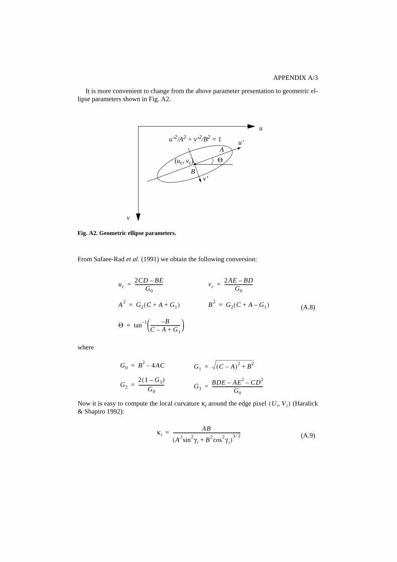
APPENDIX A/3
It is more convenient to change from the above parameter presentation to geometric el-lipse parameters shown in Fig. A2.
From Safaee-Rad et al. (1991) we obtain the following conversion:
(A.8)
where
Now it is easy to compute the local curvature κi around the edge pixel (Haralick& Shapiro 1992):
(A.9)
u
v
A
B
Θ.(uc, vc)
Fig. A2. Geometric ellipse parameters.
u’2/A2 + v’2/B2 = 1 u’
v’
uc2CD BE–
G0-------------------------= vc
2AE BD–G0
-------------------------=
Θ tan 1– B–C A– G1+---------------------------
=
A 2 G2 C A G1+ +( )= B 2 G2 C A G1–+( )=
G0 B2 4AC–= G1 C A–( )2 B2+=
G2
2 1 G3–( )G0
-----------------------= G3BDE AE2– CD2–
G0----------------------------------------------=
Ui V i,( )
κiAB
A 2sin2γ i B 2cos2γ i+( )3 2⁄-------------------------------------------------------------=

APPENDIX A/4
where
The coefficient ai is estimated from the local curvature κi. It can be easily shown that thecurvature of a parabola at the extreme point is 2ai. We may use this relation so that
(A.10)
The next problem is to determine the parameters di and x0, i based on Ai, gu, i, gv, i, andai. Two cases, also illustrated in Fig. 7a and Fig. 7b, are considered. In the first case, theparabola is limited to the opposite margins of the detection window, and in the second casethe parabola covers only one corner of the window. Therefore, we first need to discriminatebetween these two cases, and then calculate the correction for the edge pixels. The follow-ing procedure is performed for each edge pixel :
Step 1 compute , A0, i, and di
Step 2 discriminate between cases a and b
if di ≥ 0 select Step 3a, otherwise select Step 3b
cos2γ i
Ui uc–( ) Θcos V i vc–( ) Θsin+( )2
Ui uc–( )2 V i vc–( )2+-----------------------------------------------------------------------------------=
sin2γ i
V i vc–( ) Θ Ui uc–( ) Θsin–cos( )2
Ui uc–( )2 V i vc–( )2+----------------------------------------------------------------------------------=
ai
κi
2----=
Ui V i,( )
x0 i,
x0 i,
n2 gv i,-------------- gu i, gv i,≤,
n2 gu i,-------------- otherwise,
=
A0 i,
43---aix0 i,
3 n2gu i,
2gv i,--------------+ gu i, gv i,≤,
43---aix0 i,
3 n2gv i,
2gu i,--------------+ otherwise,
=
di
Ai A0 i,–( )n
-------------------------=

APPENDIX A/5
Step 3a compute the refined edge position .
Step 3b compute ρi and ti, recompute
compute the refined edge position .
Notice that the parameter ti in Step 3b may have a complex value due to a negative resultinside the square-root term. However, is always a real number. An example of the re-fined edge point locations is shown in Fig. A1c.
ui vi,( )
ui
Ui aigu i, x0 i,2 gu i, gv i,≤,–
Uin2--- 1 gv i,
gu i,--------–
di– sign gu i,( ) aigu i, x0 i,2 otherwise,–+
=
vi
V in2--- 1 gu i,
gv i,--------–
di– sign gv i,( ) aigv i, x0 i,2– gu i, gv i,≤,+
V i aigv i, x0 i,2 otherwise,–
=
x0 i,
ρi 2 gu i, gv i,=
ti
24Aiai2 ρi
3– 4ai 3Ai 12Aiai2 ρi
3–( )+
ai3
------------------------------------------------------------------------------------------=
x0 i,ai
2ti2 3⁄
ρiaiti1 3⁄ ρi
2+–
4ai2ti
1 3⁄---------------------------------------------------=
ui vi,( )
ui Uin2--- x0 i, gv i,–
sign gu i,( ) aigu i, x0 i,2–+=
vi V in2--- x0 i, gu i,–
sign gu i,( ) aigv i, x0 i,2–+=
x0 i,

APPENDIX B/1
Appendix B: Renormalization
The purpose of Appendix B is to describe the algorithm for performing the renormalizationconic fitting. The theoretical background is not represented here. For more information, seeKanatani (1994) and Zhang (1995). The bias-corrected procedure is adopted from Zhang(1995), where the ellipse has the following representation:
(B.1)
The unknown parameters constitute the vector p = [A, B, C, D, E, F]T. It is assumed thatthe elliptic feature consists of N edge points (ui, vi), where i = 1,..., N. The following stepsare performed:
Step 1 Let c = 0, wi = 1 for i = 1,..., N.
Step 2 Compose the matrix
where
and
Au2 2Buv Cv2 2Du 2Ev F+ + + + + 0=
N
N wi Ni cBi–[ ]i 1=
N
∑=
Ni
ui4 2ui
3vi ui2vi
2 2ui3 2ui
2vi ui2
2ui3vi 4ui
2vi2 2uivi
3 4ui2vi 4uivi
2 2uivi
ui2vi
2 2uivi3 vi
4 2uivi2 2vi
3 vi2
2ui3 4ui
2vi 2uivi2 4ui
2 4uivi 2ui
2ui2vi 4uivi
2 2vi3 4uivi 4vi
2 2vi
ui2 2uivi vi
2 2ui 2vi 1
=

APPENDIX B/2
Step 3 Compute the unit eigenvector of associated to the smallest eigenvalue, whichis denoted by λmin ( is the estimate of p).
Step 4 Update c as
Step 5 Recompute wi using the new
Step 6 Return if the update has converged, otherwise go back to Step 2.
The quadratic form in Eq. (2.11) is slightly different from Eq. (B.1) used by Zhang. There-fore it is necessary to perform the following conversion in order to obtain consistent resultswith other algorithms described in this thesis:
It should be noticed that the algorithm represented provides an unbiased estimate of the el-lipse parameters. However, it is not guaranteed that the estimator is the most efficient, i.e.,the minimum variance of the estimation error is not necessarily achieved.
Bi
6ui2 6uivi ui
2 vi2+ 6ui 2vi 1
6uivi 4 ui2 vi
2+( ) 6uivi 4vi 4ui 0
ui2 vi
2+ 6uivi 6vi2 2ui 6vi 1
6ui 4vi 2ui 4 0 0
2vi 4ui 6vi 0 4 0
1 0 1 0 0 0
=
p Np
c cλmin
pTwiBipi 1=
N∑-------------------------------------+←
p
wi 1 A2
B2
+( )ui2 B
2C
2+( )+[⁄ vi
2 2B A C+( )uivi+=
2 AD BE+( )ui 2 BD CE+( )vi D2
E2
+( ) ]+ ++
p
A A← B 2B←
C C← D 2D←
E 2E←F F←