accurate 3d image colour histogram transformation

Accurate 3D image colour histogram transformation

J�aan Morovic a,*, Pei-Li Sun a,b

a Colour and Imaging Institute, University of Derby, Kingsway House, Kingways, Derby DE22 3HL, UKb Department of Graphic Communications and Technology, Shih Hsin University, Taiwan, ROC

Abstract

Amethod for transforming an image�s 3D colour histogram to make it accurately match a predetermined target state

is described here. This method involves colour quantisation, clustering and the EMD histogram difference metric to

provide a transformation LUT between original and target histograms.

� 2002 Elsevier Science B.V. All rights reserved.

Keywords: Histogram specification; Histogram matching; Histogram transformation; 3D colour histogram

1. Introduction

Various imaging applications, such as colour

reproduction or image database retrieval algo-rithms, perform better for some images than for

others and can therefore be thought of as having

image-dependent performance. Being able to trans-

form image characteristics in a direct, arbitrary

and accurate way can then help with studying the

nature of this image-dependence of imaging ap-

plications.

To understand what impact a given imagecharacteristic (IC) has on the performance of someapplication it is useful to have two sets of images

with the following properties: first, a set of images

that differ in many characteristics (multi-IC) and

where the given application performs differently

for its different members. Second, a set that does

not differ in one characteristic (equi-IC) but does

differ in all other unrelated image characteristics

just like multi-IC. What is meant here by unrelated

image characteristics are those whose states arenot determined by the given image characteristic.

For example, changing an image�s colour gamut

also determines its lightness range but not its

content. Hence gamut and lightness range are re-

lated and gamut and content are unrelated image

characteristics. If the application then varies less

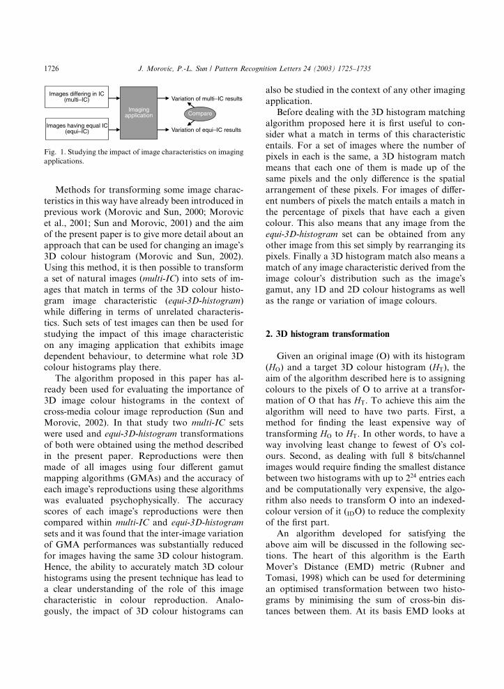
for equi-IC than for multi-IC (Fig. 1), then it is

dependent on image characteristic IC (Morovicand Sun, 1999).

The challenge in the above approach is that

equi-IC sets are difficult to populate with �natural�images, whereby what is meant here by �natural�images are those that directly result from image

capture or generation and look unperturbed or

�normal�. An alternative therefore is to generate

equi-IC sets computationally from multi-IC sets.However, to do this it is necessary to be able to

transform image characteristics in controlled ways.

*Corresponding author. Tel.: +44-1332593101; fax: +44-

1332622218.

E-mail address: [email protected] (J. Morovic).

0167-8655/03/$ - see front matter � 2002 Elsevier Science B.V. All rights reserved.

doi:10.1016/S0167-8655(02)00328-8

Pattern Recognition Letters 24 (2003) 1725–1735

www.elsevier.com/locate/patrec

mail to: [email protected]

Methods for transforming some image charac-

teristics in this way have already been introduced in

previous work (Morovic and Sun, 2000; Morovic

et al., 2001; Sun and Morovic, 2001) and the aimof the present paper is to give more detail about an

approach that can be used for changing an image�s3D colour histogram (Morovic and Sun, 2002).

Using this method, it is then possible to transform

a set of natural images (multi-IC) into sets of im-

ages that match in terms of the 3D colour histo-

gram image characteristic (equi-3D-histogram)

while differing in terms of unrelated characteris-tics. Such sets of test images can then be used for

studying the impact of this image characteristic

on any imaging application that exhibits image

dependent behaviour, to determine what role 3D

colour histograms play there.

The algorithm proposed in this paper has al-

ready been used for evaluating the importance of

3D image colour histograms in the context ofcross-media colour image reproduction (Sun and

Morovic, 2002). In that study two multi-IC sets

were used and equi-3D-histogram transformations

of both were obtained using the method described

in the present paper. Reproductions were then

made of all images using four different gamut

mapping algorithms (GMAs) and the accuracy of

each image�s reproductions using these algorithmswas evaluated psychophysically. The accuracy

scores of each image�s reproductions were then

compared within multi-IC and equi-3D-histogram

sets and it was found that the inter-image variation

of GMA performances was substantially reduced

for images having the same 3D colour histogram.

Hence, the ability to accurately match 3D colour

histograms using the present technique has lead toa clear understanding of the role of this image

characteristic in colour reproduction. Analo-

gously, the impact of 3D colour histograms can

also be studied in the context of any other imaging

application.

Before dealing with the 3D histogram matching

algorithm proposed here it is first useful to con-

sider what a match in terms of this characteristic

entails. For a set of images where the number ofpixels in each is the same, a 3D histogram match

means that each one of them is made up of the

same pixels and the only difference is the spatial

arrangement of these pixels. For images of differ-

ent numbers of pixels the match entails a match in

the percentage of pixels that have each a given

colour. This also means that any image from the

equi-3D-histogram set can be obtained from anyother image from this set simply by rearranging its

pixels. Finally a 3D histogram match also means a

match of any image characteristic derived from the

image colour�s distribution such as the image�sgamut, any 1D and 2D colour histograms as well

as the range or variation of image colours.

2. 3D histogram transformation

Given an original image (O) with its histogram

(HO) and a target 3D colour histogram (HT), the

aim of the algorithm described here is to assigning

colours to the pixels of O to arrive at a transfor-

mation of O that has HT. To achieve this aim the

algorithm will need to have two parts. First, amethod for finding the least expensive way of

transforming HO to HT. In other words, to have a

way involving least change to fewest of O�s col-

ours. Second, as dealing with full 8 bits/channel

images would require finding the smallest distance

between two histograms with up to 224 entries each

and be computationally very expensive, the algo-

rithm also needs to transform O into an indexed-colour version of it (IDO) to reduce the complexity

of the first part.

An algorithm developed for satisfying the

above aim will be discussed in the following sec-

tions. The heart of this algorithm is the Earth

Mover�s Distance (EMD) metric (Rubner and

Tomasi, 1998) which can be used for determining

an optimised transformation between two histo-grams by minimising the sum of cross-bin dis-

tances between them. At its basis EMD looks at

Images differing in IC(multi–IC)

Imagingapplication

Variation of multi–IC results

Compare

Variation of equi–IC resultsImages having equal IC

(equi–IC)

Fig. 1. Studying the impact of image characteristics on imaging

applications.

1726 J. Morovic, P.-L. Sun / Pattern Recognition Letters 24 (2003) 1725–1735

histogram differences as cases of the transporta-

tion problem (Hitchcock, 1941). The transporta-

tion problem deals with cases where there are

several suppliers, each with a certain amount of

some goods, who are to supply several customers,

each with a given capacity and location. The taskis then to find the least expensive flow of goods

taking into account both the amount transported

and the distance across which it is moved.

Applying this to histograms, an original histo-

gram�s values can be seen as amounts of suppliers�goods and the target histogram�s values as the

customers� demands whereby the task is to fill the

customers� demands with the suppliers� goods inthe most economical way. Histogram difference

can then be expressed in terms of how ‘‘expensive’’

it is to transform one histogram into another. The

calculation of such a histogram metric can then be

formalised as a linear programming problem with

constraints on the kind of movements allowed.

The linear programming problem can be for-

malised as follows:

workðHO;HT; F Þ ¼Xmi¼1

Xn

j¼1ðdijfijÞ ð1Þ

Here, HO and HT represent original and target

histograms with a total number of m and n bins,

respectively. dij represents the distance (i.e., DEcolour difference) between the ith colour repre-

sentative in HO and the jth colour representative inHT, and fij is the flow between the two colour

representatives. The task is to find a flow F ¼ ½fij�to minimise the overall cost work ðHO;HT; F Þsubject to the following constrains (where wOi and

wTj represent the colour frequencies in the ith and

the jth bins of histogram HO and HT, respectively):

(1) fij P 0 16 i6m; 16 j6 n

(2)Pn

j¼1 fij 6wOi 16 i6m

(3)Pm

i¼1 fij 6wTj 16 j6 n

(4)Pm

i¼1Pn

j¼1 fij ¼ minPm

i¼1 wOi;Pn

j¼1 wTj

� �

Constraint (1) allows moving ‘‘supplies’’ from

HO to HT and not vice versa. Constraint (2) limits

the amount of supplies that can be sent by the

colours in HO to their colour frequencies (wOi).Constraint (3) limits the colours in HT to receive

no more supplies than their colour frequencies

(wTj); and constraint (4) forces to move the maxi-

mum amount of supplies possible between each

pair of original and target bins. Furthermore,

using a DE colour difference formula for evaluat-

ing cross-bin distances for colour pairs from a pairof 3D image colour histograms allows for the

transformation to take into account models of

colour and colour difference perception.

The reason for using the EMD histogram dif-

ference metric in the present method is that it gives

great control over how cross-bin differences are

determined. Unlike other methods, such as exact

histogram matching––EHM (Morovic et al., 2001)or the sort-matching algorithm (Rolland et al.,

2000), it is not necessary for the bins to be in a

specific order or even for it to be possible to order

them. It means that EMD can be used for trans-

forming 3D histograms by representing them as

1D histograms and by not having to use the 1D

histogram�s bin indices for computing cross-bin

differences. Instead EMD allows for these differ-ences to be computed based on the 3D colour

coordinates corresponding to each 1D bin index.

The following are then the steps of this algo-

rithm for transforming an image to have a pre-

determined 3D colour histogram in terms of a

perceptually uniform colour space. Note also that

throughout the remainder of the paper a set of

four original images and their transformations willbe used for illustrating the algorithm. This set of

images is shown in the top-left to bottom-right

diagonal of Fig. 7 and consists of CG––a com-

puter graphic, MUS––an indoor photographic

image showing a group of musicians, SKI––an

indoor photographic image showing ski wear and

STR––an outdoor photographic image showing a

street scene.Step 1. Computing colour appearance. Given an

original 24-bit image with RGB values for its

pixels and displayed on a computer display, the

first step is to compute the colour appearance at-

tributes for each of its pixels. This will allow for

the following steps to be performed in a space that

is perceptually more uniform than the RGB space

of the display and therefore allow for all parts ofcolour space to be given similar weights. CAM97s2

(Li et al., 2000) was used here for predicting the

J. Morovic, P.-L. Sun / Pattern Recognition Letters 24 (2003) 1725–1735 1727

colour appearances of image pixels in terms of the

Jab colour space having J as a lightness predictor

and a and b as redness–greenness and yellowness–

blueness predictors, respectively. Note that a and bare orthogonal coordinates corresponding to the

polar coordinates of chroma (C) and hue angle (h)predicted by CAM97s2. As this model predicts

appearance given tristimulus values of image pix-

els, these are computed for image RGB values

using a forward characterisation model (CM) of

the display. Since the display on which images

were shown in this study is a CRT a model like the

gain-offset-gamma (GOG) one can be used (Berns,

1996).Step 2. Reducing bit-depth. Transform the Jab

image obtained form Step 1 from 24-bits (8-bits

per channel) to 18-bits (6-bits per channel) by

performing Floyd–Steinberg error diffusion (Ulich-

ney, 1993). The reason for using this algorithm is

to reduce the sample size for the next step while

preserving most of the colour information from

the original. The ðJ ; a; bÞ intervals of the result-ing 18-bit image were ð1:57; 4; 4Þ CAM97s2 units,

which corresponds to a maximum pixel-by-pixel

Euclidean colour difference (DE97s2) between the

original and reduced bit-depth images of approx-

imately 6 units. This magnitude of difference in

turn has been previously shown to be around the

perceptibility threshold of differences between

complex images (Uroz et al., 2002) and as suchresulting differences should be at most only just

perceptible.

Step 3. Indexing colours. The 18-bit image from

Step 2 is next transformed to N indexed colours (N

values of 256, 512, 1024 and 3072 were investi-

gated in this study) using a modified Foray clus-

tering algorithm (Gose et al., 1996) whereby the

resulting N colours are chosen differently for each

image. In the clustering process, colours are added

to the cluster having the smallest Euclidean dis-tance in Jab colour space. Image histograms

(IDHs) of the N indexed colour images are then

computed whereby their data structure consists of

index number, corresponding Jab values and col-

our frequency as a percentage of total number of

pixels.

Step 4. Calculating transformation between his-

tograms. EMD is used for calculating optimalcross-bin distances between the histogram of the

original image (IDHO) and the target histogram

(IDHT). The output of EMD is then an LUT in-

dicating the net-like relationship of all bins be-

tween the two histograms (Fig. 2). For example, in

Fig. 2, original pixels having the colour repre-

sented by the first bin of the original histogram

would be transformed so that one would have thefirst, three the second and two the third bin�s col-our from the target histogram. The transformation

LUT then is an m� n matrix whereby each row

represents a given index number (IOi) from the

original histogram and the colour corresponding

to it ðJOi; aOi; bOiÞ, where i 2 f1;mg and m is the

number of bins in the original histogram. The

columns represent the target histogram and eachcolumn corresponds to a given index number (ITj)from the target histogram and the colour corres-

ponding to it (JTj; aTj; bTj), where j 2 f1; ng and nis the number of bins in the target histogram. Here

binindex freq.

6

4

1

1

2

3

binindexfreq.

2

7

2

1

2

3

IDHO DHT

24

1

13

1 0 0

0 4 0

1 3 2

IDHT

IT1JT1aT1bT1

IT2JT2aT2bT2

IT3JT3aT3bT3

IO1,JO1,aO1,bO1IO2,JO2,aO2,bO2IO3,JO3,aO3,bO3

IDHO

2 7 2

1

4

6

(a) (b)

Fig. 2. (a) Relationship between original and target histogram bins computed using EMD and DE. (Shades of each bin represent its

colour and numbers above lines connecting original and target histogram bins show how many pixels of an original index are

transformed to a given target index). (b) Transformation LUT corresponding to relationship from Fig. 2a.


both m and n were equal to N . The value at (i; j) ofthe transformation LUT then shows how many

original pixels of the ith index need to be trans-

formed to the target histogram�s jth colour. To

show that the transformation represented by the

LUT will exactly result in the transformed imagehaving the target histogram, the sum of values in

the rows shows that all original colours will be

transformed and the sum of the columns shows

that the transformed colours will have the target

histogram. As such the present method guarantees

an accurate match to the target histogram. Note

that the implementation of the EMD algorithm

used in this study was based on the source codeprovided by Rubner (2000).

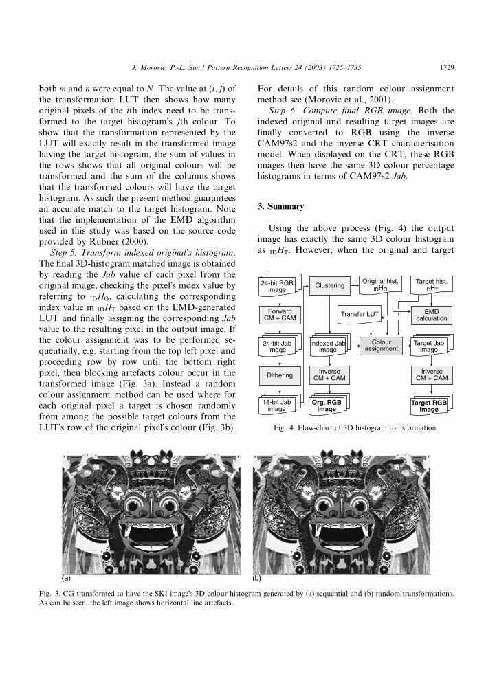
Step 5. Transform indexed original’s histogram.

The final 3D-histogram matched image is obtained

by reading the Jab value of each pixel from the

original image, checking the pixel�s index value byreferring to IDHO, calculating the corresponding

index value in IDHT based on the EMD-generated

LUT and finally assigning the corresponding Jabvalue to the resulting pixel in the output image. If

the colour assignment was to be performed se-

quentially, e.g. starting from the top left pixel and

proceeding row by row until the bottom right

pixel, then blocking artefacts colour occur in the

transformed image (Fig. 3a). Instead a random

colour assignment method can be used where for

each original pixel a target is chosen randomlyfrom among the possible target colours from the

LUT�s row of the original pixel�s colour (Fig. 3b).

For details of this random colour assignment

method see (Morovic et al., 2001).

Step 6. Compute final RGB image. Both the

indexed original and resulting target images are

finally converted to RGB using the inverse

CAM97s2 and the inverse CRT characterisationmodel. When displayed on the CRT, these RGB

images then have the same 3D colour percentage

histograms in terms of CAM97s2 Jab.

3. Summary

Using the above process (Fig. 4) the outputimage has exactly the same 3D colour histogram

as IDHT. However, when the original and target

Org. RGBimage

Target RGBimage

24-bit RGBimage

ForwardCM + CAM

Dithering

18-bit Jabimage

Original hist.IDHO

Target hist.IDHT

EMDcalculation

Transfer LUT

Colourassignment

Target Jabimage

InverseCM + CAM

Indexed Jabimage

24-bit Jabimage

Clustering

InverseCM + CAM

Fig. 4. Flow-chart of 3D histogram transformation.

Fig. 3. CG transformed to have the SKI image�s 3D colour histogram generated by (a) sequential and (b) random transformations.

As can be seen, the left image shows horizontal line artefacts.


histograms are very different, the output image can

show strong artefacts and have a more ample

power spectrum in the high spatial frequency

range. In order to reduce such artefacts and to

reduce the power of high spatial frequencies, an

attempt can be made to adjust the steps of theabove procedure. The success of the attempts to

adjust some parts of the process was assessed in

terms of a local colour spatial frequency metric

and this will be introduced next.

4. Local colour spatial frequency

After performing 3D-histogram matching, the

high spatial frequencies in the power spectrum of

the histogram-perturbed image normally have

higher amplitudes than corresponding ones in the

original. It would be ideal if the histogram-

perturbed image could maintain not only the

image content of the original image but also the

power spectrum distribution of local colour spatialfrequencies (LCSFs) in it. As the original image

changes its colours totally after histogram match-

ing, no colour difference metric can estimate the

variation of its power spectrum and a separate

metric for measuring these errors has therefore

been developed.

To evaluate the variation of the power spec-

trum, both the original and histogram-perturbedJab images are first subdivided into blocks of

16� 16 pixels and 50 units are subtracted from all

the J values. Each block is then transformed to a

16� 16 spatial frequency matrix F ðu; vÞ using a

2D fast Fourier transform (FFT) for J , a and

b, respectively. The logarithmic power spectrum

log P ðu; vÞ of F ðu; vÞ is computed and averaged

across all orientations (/) and neighbouring spa-

tial frequencies (x 1) to yield a discrete 1-D

function log P ðxÞ of radial spatial frequency x.The differences between each log PðxÞ pair of

original and perturbed images are then averaged

for the whole image and the resulting difference

function D log P ðxÞ can further be reduced to a

single value D log PJab by averaging the discrete

values of D log P ðxÞ (where x ¼ 1; 2; . . . ; 11) andfinally averaging the results of the three colour

channels (J , a, and b). As the DC component (i.e.,direct current––representing the mean value of the

16� 16 pixels) of the Fourier spectrum is insensi-

tive to the change of spatial variation, the corre-

sponding error values (D log Pð0Þ) are not used for

evaluating LCSF.

D log PJab can be regarded as a metric for eval-

uating the difference between images in terms of

LCSF. The reason for using a logarithmic scale isbecause it gives the values for each spatial fre-

quency a similar weight and is therefore more

suitable for calculating overall errors. This way of

calculating LCSF is partly based on Thomson and

Foster�s (1997) application of higher-order image

statistics. Note that zero D log PJab means that bothimages have the same distribution of spatial fre-

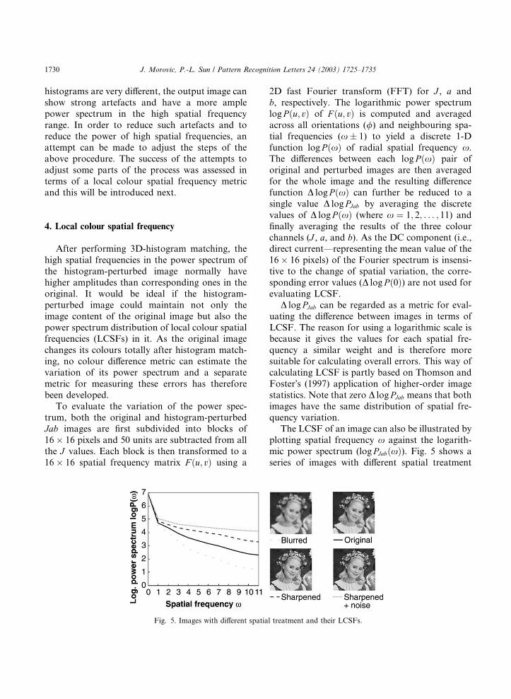
quency variation.The LCSF of an image can also be illustrated by

plotting spatial frequency x against the logarith-

mic power spectrum (log PJabðxÞ). Fig. 5 shows a

series of images with different spatial treatment

Fig. 5. Images with different spatial treatment and their LCSFs.


(blurring, sharpening and adding noise to the

original) and their corresponding LCSFs.

5. Adjusting 3D histogram matching

5.1. Choice of original and target histograms

The first factors to consider are the original and

target histograms themselves as some images

cannot be used in 3D-histogram matching without

resulting in very strong artefacts. Clearly this

would be the case when attempting a match be-

tween an image of a uniform grey wall and animage showing a colourful garden. No matter

which of these would be regarded as the original, it

would be very difficult to preserve image detail and

naturalness. Fig. 6 shows the result of matching

3D colour histograms between a business graphic

and a portrait. As can be seen, an image contain-

ing large uniform areas or non-continuous colour

distributions is not well suited as an original for3D-histogram matching. The principal problem

with transforming 3D histograms is that colour

spatial frequency tends to increase as a result of

the process. This is because neighbouring pixels of

similar colour in the original can be assigned

output colours far away from one another in Jabspace. This is particularly significant when the

colour differences between clusters in IDHT arelarger than the differences in IDHO.

5.2. Clustering and the number of indices used

As was mentioned above, a clustering technique

is used in this algorithm for generating improving

indexed-colour images. To see the effect of thisclustering, Table 1 shows the overall image colour

differences between 24-bit originals and the re-

sulting indexed-colour images. The numbers of

indices in this test were 256, 512, 1024 and 3072

and, as expected, the results showed that increas-

ing the number of indices used reduced the overall

mean-error.

5.3. Parameters affecting EMD

In the process of transforming the 3D histo-

gram of an image there are a number of para-

meters that can be adjusted and it is therefore

important to try and set them so as to reduce ar-

tefacts in the resulting histogram-transformed

images. The most important of these parametersare: (a) the maximum number of iterations; (b) the

power to which DE values are raised in EMD (i.e.

whether EMD minimises DE or DEn); (c) the

weights of DJ , DC and DH in the DE formula and

(d) the number of indices used for colour quanti-

sation.

5.3.1. Maximum number of iterations

In the EMD algorithm, the total of indexed

colour distances is minimised using an iterative

process and the maximum number of iterations

therefore plays an important role in this optimi-

sation. The artefacts of histogram-transformed

images can be reduced by increasing the maximum

number of iterations. However, the processing

becomes extremely time-consuming when thenumber of indices is large for an image. The

Fig. 6. 3D-histogram matching between a business graphic and

a portrait. (Left) Originals; (Right) histogram-matched images.

Table 1

Effect of number of indices on difference from 24-bit original

Number

of indices

Pixel-by-pixel DE97s2

Mean S.D. 95th Max.

256 3.99 2.34 11.76 27.30

512 3.64 1.96 10.02 24.36

1024 3.32 1.68 8.48 21.35

3072 2.94 1.29 6.28 18.79


maximum numbers of iterations were therefore set

to 2000, 3000, 6000 and 12,000 for the four index

numbers (256, 512, 1024 and 3072), respectively.

5.3.2. DE minimised by EMD

To evaluate the effect of varying the power ofDE in the EMD calculation, DE, DE2 and DE3 were

used for generating all the histogram matching

images by using images with 512 indexed colours

and overall results in terms of D log PJab were 0.69,0.64 and 0.68, respectively. This means that in

general the LCSF difference between original and

histogram-perturbed image pairs was somewhat

reduced by using the DE2 function. As somestudies suggest that weighted DE formulae are

preferred for gamut clipping (Katoh and Ito, 1996)

a DE2wt (1:2:1) function was also evaluated with

EMD where the weights dividing ½DJ ;DC;DH �were ½1; 2; 1�. The testing process was the same as

used above and the resulting D log PJab for DE2wt

(1:2:1) was 0.65, however, as this metric was lower

for the unweighted DE2 the latter should be used.

5.3.3. Number of indices

Different numbers of indices were also tested

(256, 512, 1024 and 3072) and this showed that

using 1024 bins gives the best result (Table 2). As

can be seen, using 3072 indexed colours did not

improve the quality of resulting images and even

though there was not much difference between 256and 1024 indices in terms of this metric, using 1024

indices improved pixel-by-pixel difference signifi-

cantly as compared with 256 indices (Table 1). A

possible reason for this is that colours of uniform

areas in the original were transformed to have a

larger number of target colours when increasing

the index numbers. Hence, the uniformity of some

areas in the original can be reduced more dra-

matically if there is a greater number of target

indexed colours assigned to them and if these in-

dexed colours are from different parts of colour

space.

6. Applying 3D histogram matching

One way of using the 3D histogram matching

technique described above is to take a set of nat-

ural images and transform each of them so as to

give it the histogram of the other images in the set.

This will result in a matrix of images as shown inFig. 7, where all the images in a given column have

the same image content (i.e. they show the same

scene) and all the images in the same row have the

same 3D colour histogram. In other words, all

images in the same row are made up of the same

pixels––the only difference between them is the

spatial arrangement of the pixels. A set like this

could, for example, be used for understandingwhat the relative importance of the 3D colour

histogram is compared to image content and this

could be seen by looking at the variation of some

imaging application�s performance for the imagesin the rows versus the columns of the matrix.

Furthermore this matrix also yields two sets of

images that each has the same image contents as

well as same 3D histograms in them. The first seton the diagonal from top left to bottom right has a

match between content and original histogram.

The second set on the other diagonal has a dif-

ferent, artificial link between content and histo-

gram. In other words, in this set each image

content is represented using the histogram of an-

other original image. Comparing these two sets

Table 2

Effect of changing number of indexed colour used in terms of D log PJab. Refer to Fig. 7, CG-to-MUS here, for instance, means the

LCSF difference between CG(org.) and CG-to-MUS images

No. of indices To-MUS To-SKI Overall

CG SKI STR CG MUS STR

256 0.40 0.12 0.64 0.63 0.95 1.05 0.633

512 0.43 0.11 0.62 0.67 0.95 1.09 0.645

1024 0.41 0.12 0.66 0.66 0.95 0.99 0.632

3072 0.40 0.33 0.85 0.75 1.12 1.16 0.766


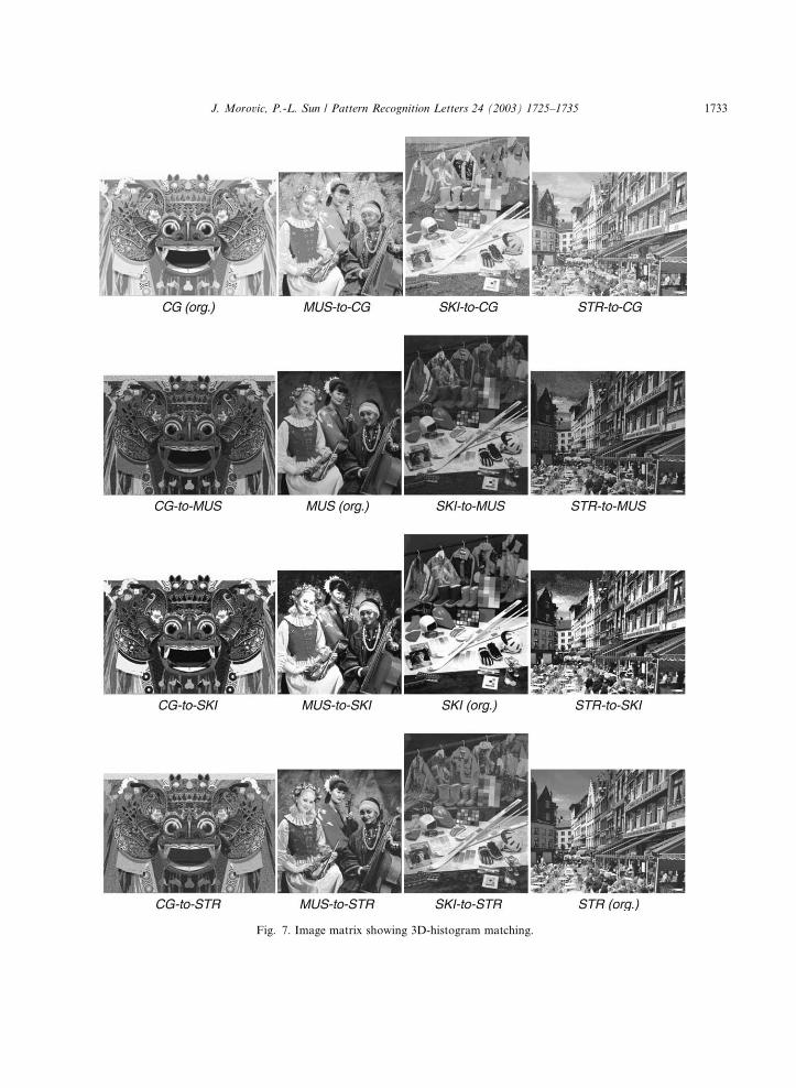
Fig. 7. Image matrix showing 3D-histogram matching.


can show whether there is any connection betweencontent and 3D histogram from the point of view

of some imaging application. In other words, if the

performance of an imaging application is the same

for corresponding members of these two sets, then

it is the 3D histogram that plays the most impor-

tant role, whereas if there are significant differences

then image content as such has more impact.

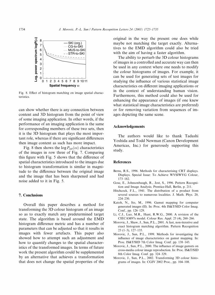
Fig. 8 then shows the log PJabðxÞ characteristicsof the images in row three of Fig. 7. Comparing

this figure with Fig. 5 shows that the difference of

spatial characteristics introduced to the images due

to histogram transformation is similar in magni-

tude to the difference between the original image

and the image that has been sharpened and had

noise added to it in Fig. 5.

7. Conclusions

Overall this paper describes a method for

transforming the 3D colour histogram of an image

so as to exactly match any predetermined target

state. The algorithm is based around the EMD

histogram difference metric and has a number ofparameters that can be adjusted so that it results in

images with fewer artefacts. This paper also

showed how to attempt such an adjustment and

how to quantify changes to the spatial character-

istics of the transformed images. In terms of future

work the present algorithm could be supplemented

by an alternative that achieves a transformation

that does not change the spatial properties of the

original in the way the present one does while

maybe not matching the target exactly. Alterna-

tives to the EMD algorithm could also be tried

with the aim of having a faster algorithm.

The ability to perturb the 3D colour histograms

of images in a controlled and accurate way can thenbe used in any context where one needs to modify

the colour histograms of images. For example, it

can be used for generating sets of test images for

studying the influence of various statistical image

characteristics on different imaging applications or

in the context of understanding human vision.

Furthermore, this method could also be used for

enhancing the appearance of images (if one knewwhat statistical image characteristics are preferred)

or for removing variation from sequences of im-

ages depicting the same scene.

Acknowledgements

The authors would like to thank TadashiYoshida and Todd Newman (Canon Development

Americas, Inc.) for generously supporting this

study.

References

Berns, R.S., 1996. Methods for characterising CRT displays.

Displays. Special Issue: To Achieve WYSIWYG Colour,

173–182.

Gose, E., Johnsonbaugh, R., Jost, S., 1996. Pattern Recogni-

tion and Image Analysis. Prentice-Hall, Berlin, p. 211.

Hitchcock, F.L., 1941. The distribution of a product from

several sources to numerous localities. J. Math. Phys. 20,

224–230.

Katoh, N., Ito, M., 1996. Gamut mapping for computer

generated images (II). In: Proc. 4th IS&T/SID Color Imag.

Conf., pp. 126–129.

Li, C.J., Luo, M.R., Hunt, R.W.G., 2000. A revision of the

CIECAM97s model. Colour Res. Appl. 25 (4), 260–266.

Morovic, J., Shaw, J., Sun, P.L., 2001. A fast, non-iterative and

exact histogram matching algorithm. Pattern Recognition

23 (1–3), 127–135.

Morovic, J., Sun, P.L., 1999. Methods for investigating the

influence of image characteristics on gamut mapping. In:

Proc. IS&T/SID 7th Color Imag. Conf. pp. 138–143.

Morovic, J., Sun, P.L., 2000. The influence of image gamuts on

cross-media colour image reproduction. In: Proc. IS&T/SID

8th Color Imag. Conf. pp. 324–329.

Morovic, J., Sun, P.L., 2002. Transforming 3D colour histo-

grams of images. In: CGIV 2002 Proc., pp. 104–108.

Fig. 8. Effect of histogram matching on image spatial charac-

teristics.


Rolland, J.P., Vo, V., Bloss, B., Abbey, C.K., 2000. Fast

algorithm for histogram matching: application to texture

synthesis. J. Electron. Imag. 9 (1), 39–45.

Rubner, Y., 2000. EMD source-code. Available from http://

robotics.stanford.edu/�rubner/emd/default.htm.Rubner, Y., Tomasi, C., 1998. Comparing the EMD with

other dissimilarity measures for color images. In: Proc.

DARPA Image Understanding Workshop, pp. 331–

339.

Sun, P.L., Morovic, J., 2001. The Influence of image histograms

on cross-media colour image reproduction. In: PICS 2001

Montr�eeal, Canada, pp. 363–367.

Sun, P.L., Morovic, J., 2002. 3D Histograms in Colour Image

Reproduction. Proc. SPIE 4663, pp. 51–62.

Thomson, M.G.A., Foster, D.H., 1997. Role of second- and

third-order statistics in discriminability of natural images.

J. Opt. Soc. Amer. A 14 (9), 2081–2090.

Ulichney, R., 1993. In: Digital Halftoning. MIT Press,

Cambridge, MA, p. 241.

Uroz, J., Morovic, J., Luo, M.R., 2002. Perceptibility thresh-

olds of colour differences in large printed images. In:

MacDonald, L.W., Luo, M.R. (Eds.), Colour Image Science

Exploiting Digital Media. John Wiley & Sons, New York,

pp. 49–73.


http://robotics.stanford.edu/~rubner/emd/default.htm



accurate 3d image colour histogram transformation

Documents