accuracy of acoustic velocity metering systems for measurement of

ACCURACY OF ACOUSTIC VELOCITY METERING SYSTEMS FOR MEASUREMENT OF LOW VELOCITY IN OPEN CHANNELS

By Antonius Laenen and R.E. Curtis, Jr.

U.S. GEOLOGICAL SURVEY Water-Resources Investigations Report 89-4090

Prepared in cooperation with theSOUTH FLORIDA WATER MANAGEMENT DISTRICT

Tallahassee, Florida 1989

DEPARTMENT OF THE INTERIOR

MANUEL LUJAN, JR., Secretary

U.S. GEOLOGICAL SURVEY

Dallas L. Peck, Director

For additional information Copies of this report can bewrite to: purchased from:

District Chief Books and Open-File ReportsU.S. Geological Survey U.S. Geological SurveySuite 3015 Federal Center, Building 810227 North Bronough Street Box 25425Tallahassee, Florida 32301 Denver, Colorado 80225

CONTENTS

PageAbstract ------------------------------------------------------------------ 1Introduction --------------------------------------------------------------- 1Theory of signal processing ---------------------------------------------------- 2Error sources -------------------------------------------------------------- 2

Equipment error ------------------------------------------------------- 3Signal detection ----------------------------------------------------- 4Timing oscillator ---------------------------------------------------- 4

Environmental error ----------------------------------------------------- 5Angle error -------------------------------------------------------- 5Path-length error ---------------------------------------------------- 5Ray-bending error --------------------------------------------------- 6Changes to vertical-velocity profile --------------------------------------- 6

Laboratory and field tests of acoustic velocity metering systems -------------------------- 7Tow-tank test ---------------------------------------------------------- 7Field test ------------------------------------------------------------- 12

Summary and conclusions ----------------------------------------------------- 14References cited ------------------------------------------------------------ 15

ILLUSTRATIONS

Page

Figures 1-2. Diagrams showing:1. Velocity components used in traveltime equation ------------------------ 32. Voltage representation of upstream and downstream transmit and

receive pulses ----------------------------------------------- 3

3-6. Photographs of:3. Tow tank at U.S. Geological Survey hydraulic laboratory ------------------- 84. Acoustic velocity meter transducers mounted on tow-tank cart -------------- 85. Tow-tank cart holding acoustic velocity meter equipment ------------------ 96. Acoustic velocity meter transducer mounts installed on a concrete structure

after a field test of the equipment --------------------------------- 12

TABLESPage

Table 1. Timing and velocity error for different path lengths and transducer frequencies forone interrogation per measurement, based on an assumed signal-detection error of one-quarter cycle of the transducer frequency --------------------------- 4

2. Velocity error for various path lengths related to the frequency of the timing oscillator(80 megahertz) for one interrogation per measurement --------------------- 5

3. Velocity error in percent for error in path angle for various path angles ----------- 64. Percent error in distance caused by various errors in temperature measurement for

various temperatures --------------------------------------------- 6

5. Velocity error in percent caused by various temperature and specific conductancegradients for various acoustic velocity meter path lengths ------------------- 7

6. Acoustic velocity meter (AVM) and tow-tank cart velocities for 1-minute intervalsusing mismatched 200-kilohertz transducers ----------------------------- 10

7. Acoustic velocity meter (AVM) and tow-tank cart velocities for 1-minute intervalsusing matched 200-kilohertz transducers ------------------------------- 11

8. Acoustic velocity meter (AVM) and current-meter measurement (CMM) velocitiesin a field test of an acoustic velocity meter system placed in a concrete structure - - - 13

111

ACCURACY OF ACOUSTIC VELOCITY METERING SYSTEMS FOR MEASUREMENT OF LOW VELOCITY IN OPEN CHANNELS

By Antonius Laenen and R.E. Curtis, Jr.

ABSTRACT

The accuracy of acoustic velocity meters depends on equipment limitations, the accuracy of acoustic-path length and angle determination, and the stability of the mean velocity to acoustic-path velocity relation.

Equipment limitations depend on the path length and angle, the transducer frequency, the timing oscillator frequency, and the signal-detection scheme, 'typically, an acoustic velocity meter using a multiple-voltage threshold signal-detection scheme, 200-kilohertz transducers, an 80-megahertz timing oscillator, and averaging 100 interrogations per minute can have a velocity error of about ± 10 millimeters per second for a 20-meter path length and a velocity error of about ±1 millimeter per second for a 200-meter path length.

Error in the measurement of acoustic-path angle or length can result in a proportional measurement bias. Typically, an angle error of 1 degfee can result in a velocity error of 2 percent, and a path-length error of 1 meter in 100 meters can result in an error of 1 percent. In many situations, these measurement errors can be adjusted with check current-meter measurements. For very low velocity flow where check measurements are impractical, special care must be taken to make the best possible path angle and length determinations.

Ray bending (signal refraction) depends on path length and density gradients present in the stream. Any deviation from a straight acoustic path between transducers can change the unique relation between path velocity and mean velocity. These deviations can then introduce error in the mean velocity computation. In many short-path situations (less than 200 meters), this error can be avoided or is of minimal importance. Typically, for a 200-meter path length, the resultant error is less than 1 percent, but for a 1,000-meter path length, the error can be greater than 10 percent.

Recent laboratory and field tests at the U.S. Geological Survey hydraulic laboratory facility at the Stennis Space Center in Mississippi have sub stantiated assumptions of equipment limitations.

An acoustic velocity meter was tested in both tow-tank and field installations. Tow-tank tests, based on the use of an acoustic velocity meter with a 4.69-meter path, had a maximum velocity error of 27 millimeters per second and an average standard deviation of 9 millimeters per second; and the field tests, also based on the use of an acoustic velocity meter with a 20.5-meter path, had a maximum velocity error of 8 millimeters per second and an average standard deviation of 4 millimeters per second.

INTRODUCTION

An acoustic velocity meter (AVM, sometimes referred to as an ultrasonic velocity meter UVM) measures the velocity of flowing water by means of a sonic or ultrasonic signal that moves faster downstream than upstream. Meters of this type are useful in determining discharge at streamflow sites where the relation between discharge and stage varies with time. The AVM is an electronic device that is capable of measur ing lower velocities than can be measured with a conventional, mechanical current meter. It can provide continuous and accurate readings of water velocity along a horizontal plane across a stream. Measurements made with these systems have been recognized as being both reliable and accurate (International Organization for Standardization 1985a, b).

Theoretically, sound can be used to measure water velocity accurately, given minimal signal refraction (that is, minimal ray bending caused by density gradients in the water). The accuracy of the measurement is then entirely dependent on: (1) acoustic-signal recognition (ability to interpret the same reference point on signals that are propagated in opposite directions), (2) the velocity error of the system timing oscillator, and (3) the path length and angle. Signal shape and frequency, timing frequency, path length and angle, and refraction are all factors that need to be identified and related to accuracy.

This report was prepared in cooperation with the South Florida Water Management District to document the accuracy of velocity measurement for AVM systems. Testing of the AVM was done in tow-tank and field installations. Error sources were identified and determination of error is shown by equations.

THEORY OF SIGNAL PROCESSING

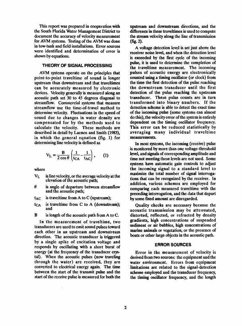
AVM systems operate on the principles that point-to-point traveltime of sound is longer upstream than downstream and that traveltimes can be accurately measured by electronic devices. Velocity generally is measured along an acoustic path set 30 to 45 degrees diagonal to streamflow. Commercial systems that measure streamflow use the time-of-travel method to determine velocity. Fluctuations in the speed of sound due to changes in water density are compensated for by the methods used to calculate the velocity. These methods are described in detail by Laenen and Smith (1983), in which the general equation (fig. 1) for determining line velocity is defined as

B2COS0 ItcA

where VL is line velocity, or the average velocity at the

elevation of the acoustic path;6 is angle of departure between streamflow

and the acoustic path;IAC is traveltime from A to C (upstream);tcA is traveltime from C to A (downstream);

andB is length of the acoustic path from A to C.

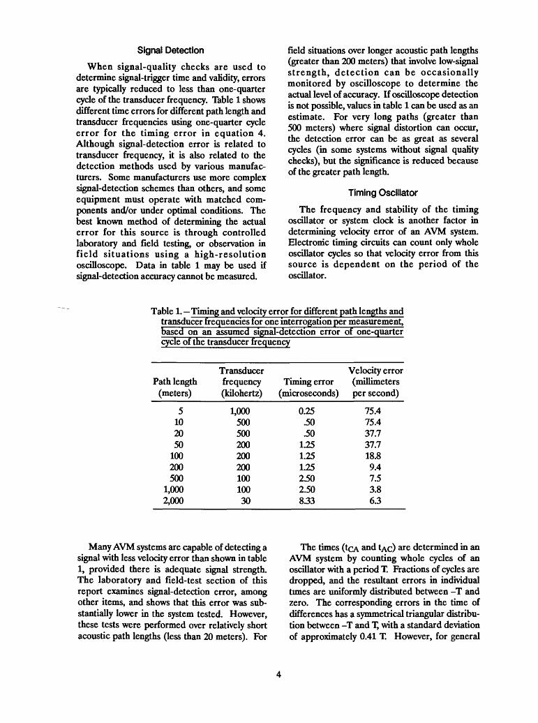
In the measurement of traveltime, two transducers are used to emit sound pulses toward each other in an upstream and downstream direction. The acoustic transducer is triggered by a single spike of excitation voltage and responds by oscillating with a short burst of energy (at the frequency of the transducer crys tal). When the acoustic pulses (now traveling through the water) are received, they are converted to electrical energy again. The time between the start of the transmit pulse and the start of the receive pulse is measured for both the

upstream and downstream directions, and the difference in these traveltimes is used to compute the stream velocity along the line of transmission (fig. 2).

A voltage detection level is set just above the receiver noise level, and when the detection level is exceeded by the first cycle of the incoming pulse, it is used to determine the completion of the traveltime measurement. The incoming pulses of acoustic energy are electronically counted using a timing oscillator (or clock) from the time the first detection of the pulse reaching the downstream transducer until the first detection of the pulse reaching the upstream transducer. These pulse counts are in turn transformed into binary numbers. If the detection scheme is able to detect the exact time of the incoming pulse (some systems can almost do this), the velocity error of the system is entirely dependent on the timing oscillator frequency. This error can be reduced statistically by averaging many individual traveltime measurements.

In most systems, the incoming (receive) pulse is monitored by more than one voltage-threshold level, and signals of corresponding amplitude and time not meeting these levels are not used. Some systems have automatic gain controls to adjust the incoming signal to a standard level to maximize the total number of signal interroga tions that can be recognized by the receiver. In addition, various schemes are employed for comparing each measured traveltime with the preceding interrogation, and the data that depart by some fixed amount are disregarded.

Quality checks are necessary because the acoustic transmission may be attenuated, distorted, reflected, or refracted by density gradients, high concentrations of suspended sediment or air bubbles, high concentrations of marine animals or vegetation, or the presence of boats or other large objects in the acoustic path.

ERROR SOURCES

Error in the measurement of velocity is derived from two sources: the equipment and the water environment. Errors from equipment limitations are related to the signal-detection scheme employed and the transducer frequency, the timing oscillator frequency, and the length

Streamflow _

-Traveltime (tAC )

(Upstream)

Transmit pulse Receive pulse

-Traveltime

(Downstream)

VTransmit pulse Receive pulse

Figure l.-Velocity components used in tiaveltime equation.Figure 2.-Voltage representation of upstream and

downstream transmit and receive pulses.

and angle of the acoustic path. Errors from environmental causes are related to the accuracy to which the distance of the acoustic path and the angle to the direction of flow can be determined, the stability of the acoustic path in the horizontal plane, and the stability of the relation between path velocity and mean velocity.

Equipment Error

In all instances, the governing equation for the determination of path velocity and error in path velocity is equation 1. For purposes of error analysis, equation 1 can be written as

VL = B2cos0 'AC'CA (2)

The equation then becomes

The velocity error resulting from errors in riming is

(4)Vcrr 2Bcos0'

whereVerr is the line velocity error (along the

horizontal plane), andten- is the error in time difference (IAC -

andB2

'AC'CAC2 ,

where C is the speed of sound with sufficient accuracy for error analysis in the ambient water.

As evidenced from equation 4, velocity errors are path-length dependent and the longer the path with the same timing error, the smaller the velocity error. In the next two sections, error will be assessed with respect to path length (path angle is assumed at 45 degrees), and the speed of sound is assumed to be 1,460 m/s.

Signal Detection

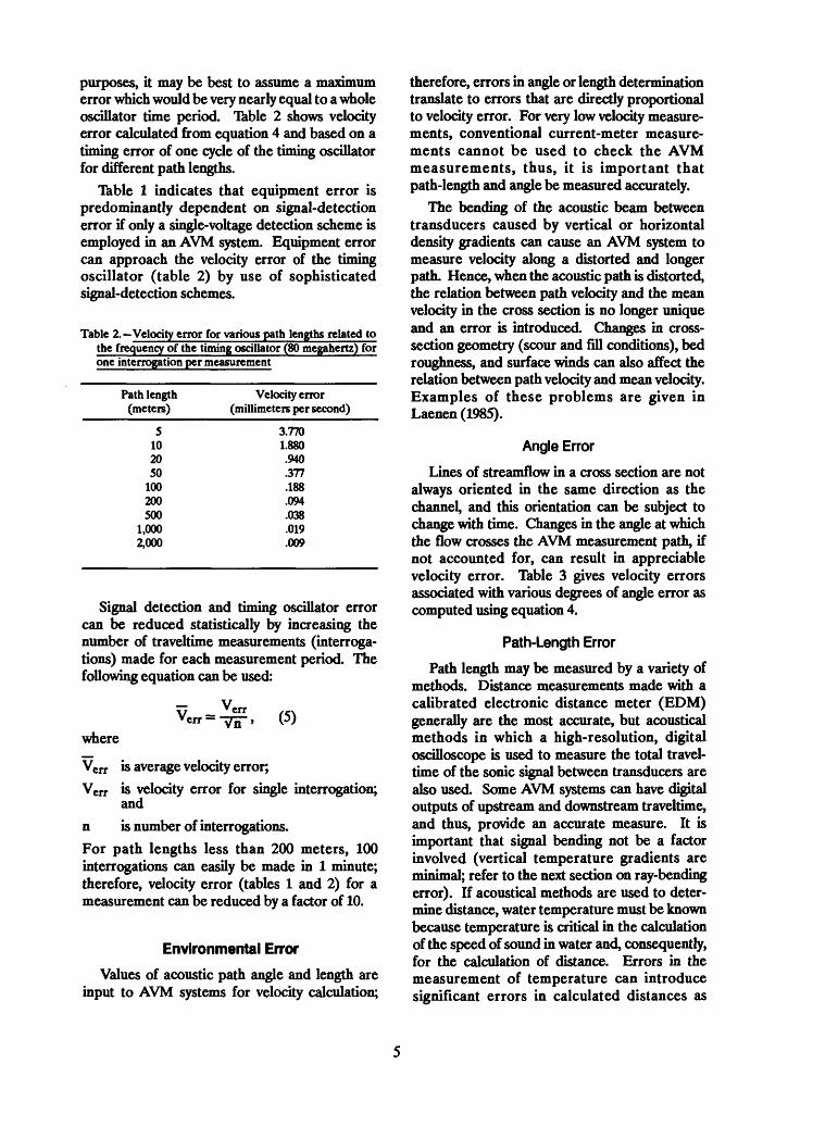
When signal-quality checks are used to determine signal-trigger time and validity, errors are typically reduced to less than one-quarter cycle of the transducer frequency. Table 1 shows different time errors for different path length and transducer frequencies using one-quarter cycle error for the timing error in equation 4. Although signal-detection error is related to transducer frequency, it is also related to the detection methods used by various manufac turers. Some manufacturers use more complex signal-detection schemes than others, and some equipment must operate with matched com ponents and/or under optimal conditions. The best known method of determining the actual error for this source is through controlled laboratory and Held testing, or observation in field situations using a high-resolution oscilloscope. Data in table 1 may be used if signal-detection accuracy cannot be measured.

field situations over longer acoustic path lengths (greater than 200 meters) that involve low-signal strength, detection can be occasionally monitored by oscilloscope to determine the actual level of accuracy. If oscilloscope detection is not possible, values in table 1 can be used as an estimate. For very long paths (greater than 500 meters) where signal distortion can occur, the detection error can be as great as several cycles (in some systems without signal quality checks), but the significance is reduced because of the greater path length.

Timing Oscillator

The frequency and stability of the timing oscillator or system clock is another factor in determining velocity error of an AVM system. Electronic timing circuits can count only whole oscillator cycles so that velocity error from this source is dependent on the period of the oscillator.

Table 1. Timing and velocity error for different path lengths and transducer frequencies for one interrogation per measurement, based on an assumed signal-detection error of one-quarter cycle of the transducer frequency

Path length (meters)

5 102050

100200500

1,000 2,000

Transducer frequency (kilohertz)

1,000 500500200200200100100 30

Timing error (microseconds)

0.25 .50.50

1.251.251.252.502.50 8.33

Velocity error (millimeters per second)

75.4 75.437.737.718.89.47.53.8 6.3

Many AVM systems are capable of detecting a signal with less velocity error than shown in table 1, provided there is adequate signal strength. The laboratory and field-test section of this report examines signal-detection error, among other items, and shows that this error was sub stantially lower in the system tested. However, these tests were performed over relatively short acoustic path lengths (less than 20 meters). For

The times (ICA *&& IAC) are determined in an AVM system by counting whole cycles of an oscillator with a period T. Fractions of cycles are dropped, and the resultant errors in individual times are uniformly distributed between -T and zero. The corresponding errors in the time of differences has a symmetrical triangular distribu tion between -T and T, with a standard deviation of approximately 0.41 T. However, for general

purposes, it may be best to assume a maximum error which would be very nearly equal to a whole oscillator time period. Table 2 shows velocity error calculated from equation 4 and based on a timing error of one cycle of the timing oscillator for different path lengths.

Table 1 indicates that equipment error is predominantly dependent on signal-detection error if only a single-voltage detection scheme is employed in an AVM system. Equipment error can approach the velocity error of the timing oscillator (table 2) by use of sophisticated signal-detection schemes.

Table 2. Velocity error for various path lengths related tothe frequency of the timing oscillator (80 megahertz) forone interrogation per measurement

Path length (meters)

5 10 20 50

100 200 500

1,000 2,000

Velocity error (millimeters per second)

3.770 1.880 .940 .377 .188 .094 .038 .019 .009

Signal detection and timing oscillator error can be reduced statistically by increasing the number of traveltime measurements (interroga tions) made for each measurement period. The following equation can be used:

r err(5)

where

'errVe

Verr

is average velocity error;is velocity error for single interrogation; and

n is number of interrogations.For path lengths less than 200 meters, 100 interrogations can easily be made in 1 minute; therefore, velocity error (tables 1 and 2) for a measurement can be reduced by a factor of 10.

Environmental Error

Values of acoustic path angle and length are input to AVM systems for velocity calculation;

therefore, errors in angle or length determination translate to errors that are directly proportional to velocity error. For very low velocity measure ments, conventional current-meter measure ments cannot be used to check the AVM measurements, thus, it is important that path-length and angle be measured accurately.

The bending of the acoustic beam between transducers caused by vertical or horizontal density gradients can cause an AVM system to measure velocity along a distorted and longer path. Hence, when the acoustic path is distorted, the relation between path velocity and the mean velocity in the cross section is no longer unique and an error is introduced. Changes in cross- section geometry (scour and fill conditions), bed roughness, and surface winds can also affect the relation between path velocity and mean velocity. Examples of these problems are given in Laenen (1985).

Angle Error

Lines of streamflow in a cross section are not always oriented in the same direction as the channel, and this orientation can be subject to change with time. Changes in the angle at which the flow crosses the AVM measurement path, if not accounted for, can result in appreciable velocity error. Table 3 gives velocity errors associated with various degrees of angle error as computed using equation 4.

Path-Length Error

Path length may be measured by a variety of methods. Distance measurements made with a calibrated electronic distance meter (EDM) generally are the most accurate, but acoustical methods in which a high-resolution, digital oscilloscope is used to measure the total traveltime of the sonic signal between transducers are also used. Some AVM systems can have digital outputs of upstream and downstream traveltime, and thus, provide an accurate measure. It is important that signal bending not be a factor involved (vertical temperature gradients are minimal; refer to the next section on ray-bending error). If acoustical methods are used to deter mine distance, water temperature must be known because temperature is critical in the calculation of the speed of sound in water and, consequently, for the calculation of distance. Errors in the measurement of temperature can introduce significant errors in calculated distances as

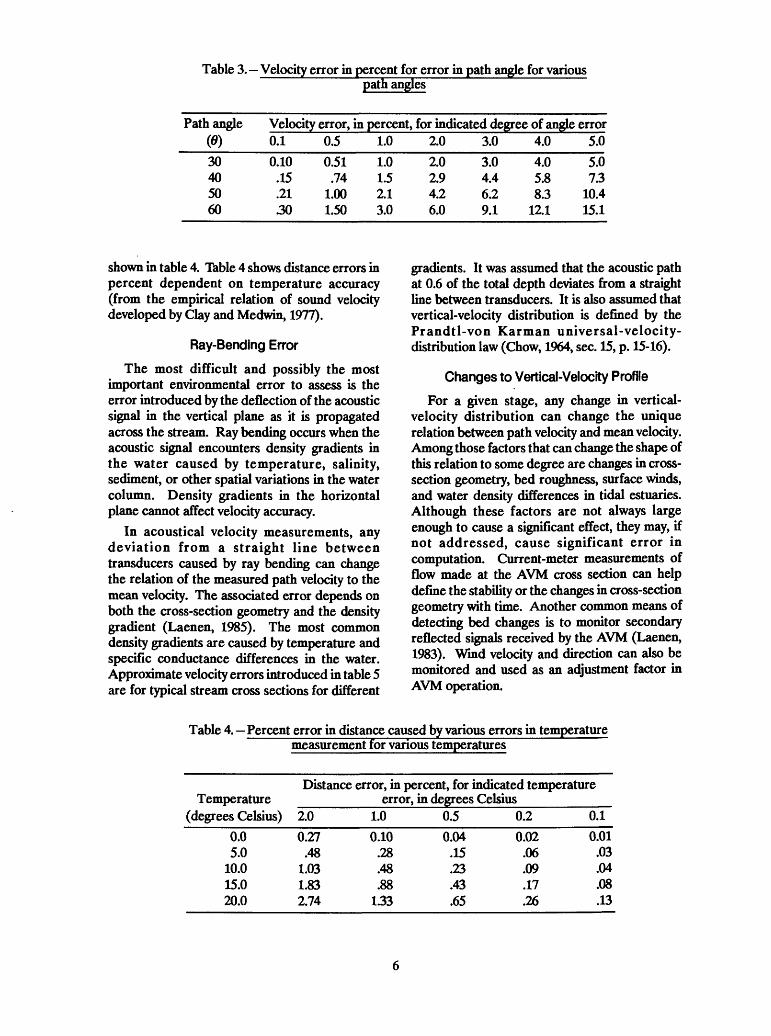
Table 3. Velocity error in percent for error in path angle for variouspath angles

Path angle Velocity error, in percent, for indicated degree of angle error(0)30405060

0.1

0.10.15.21.30

0.5

0.51.74

1.001.50

1.0

1.01.52.13.0

2.0

2.02.94.26.0

3.0

3.04.46.29.1

4.0

4.05.88.3

12.1

5.0

5.07.3

10.415.1

shown in table 4. Table 4 shows distance errors in percent dependent on temperature accuracy (from the empirical relation of sound velocity developed by Clay and Medwin, 1977).

Ray-Bending Error

The most difficult and possibly the most important environmental error to assess is the error introduced by the deflection of the acoustic signal in the vertical plane as it is propagated across the stream. Ray bending occurs when the acoustic signal encounters density gradients in the water caused by temperature, salinity, sediment, or other spatial variations in the water column. Density gradients in the horizontal plane cannot affect velocity accuracy.

In acoustical velocity measurements, any deviation from a straight line between transducers caused by ray bending can change the relation of the measured path velocity to the mean velocity. The associated error depends on both the cross-section geometry and the density gradient (Laenen, 1985). The most common density gradients are caused by temperature and specific conductance differences in the water. Approximate velocity errors introduced in table 5 are for typical stream cross sections for different

gradients. It was assumed that the acoustic path at 0.6 of the total depth deviates from a straight line between transducers. It is also assumed that vertical-velocity distribution is defined by the Prandtl-von Karman universal-velocity- distribution law (Chow, 1964, sec. 15, p. 15-16).

Changes to Vertical-Velocity Profile

For a given stage, any change in vertical- velocity distribution can change the unique relation between path velocity and mean velocity. Among those factors that can change the shape of this relation to some degree are changes in cross- section geometry, bed roughness, surface winds, and water density differences in tidal estuaries. Although these factors are not always large enough to cause a significant effect, they may, if not addressed, cause significant error in computation. Current-meter measurements of flow made at the AVM cross section can help define the stability or the changes in cross-section geometry with time. Another common means of detecting bed changes is to monitor secondary reflected signals received by the AVM (Laenen, 1983). Wind velocity and direction can also be monitored and used as an adjustment factor in AVM operation.

Table 4. Percent error in distance caused by various errors in temperature measurement for various temperatures

Distance error, in percent, for indicated temperature Temperature ________error, in degrees Celsius

(degrees Celsius)

0.0 5.0

10.0 15.0 20.0

2.0

0.27 .48

1.03 1.83 2.74

1.0

0.10 .28 .48 .88

1.33

0.50.04

.15

.23

.43

.65

0.2

0.02 .06 .09 .17 .26

0.1

0.01 .03 .04 .08 .13

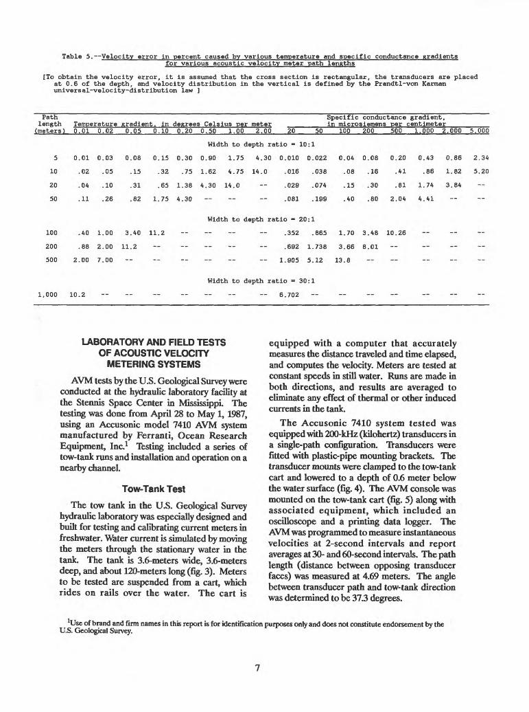
Table 5. Velocity error in percent caused by various temperature and specific conductance gradientsfor various acoustic velocity meter path lengths

[To obtain the velocity error, it is assumed that the cross section is rectangular, the transducers are placed at 0.6 of the depth, and velocity distribution in the vertical is defined by the Frandtl-von Karman universal-velocity-distribution law ]

Pathlength Temperature gradient, in degrees Celsius per meter (meters) 0.01 0.02 0.05 0.10 0.20 0.50 1.00 2.00

Specific conductance gradient, in microsiemens per centimeter

20 50 100 200 500 1.000 2.000 5.000

5 0.01 0.03 0.08

10 .02 .05 .15

20 .04 .10 .31

50 .11 .26 .82

Width to depth ratio =10:1

0.15 0.30 0.90 1.75 4.30 0.010 0.022

.32 .75 1.62 4.75 14.0 .016 .038

.65 1.38 4.30 14.0 ~ .029 .074

1.75 4.30 ~ .081 .199

0.04

.08

.15

.40

0.08

.16

.30

.80

0.20

.41

.81

2.04

0.43

.86

1.74

4.41

0.86

1.82

3.84

2.34

5.20

--

100 .40 1.00 3.40 11.2

200 .88 2.00 11.2

500 2.00 7.00


.352 .865 1.70 3.48 10.26

.692 1.738 3.66 8.01

1.905 5.12 13.8

1,000 10.2


6.702

LABORATORY AND FIELD TESTSOF ACOUSTIC VELOCITY

METERING SYSTEMS

AVM tests by the U.S. Geological Survey were conducted at the hydraulic laboratory facility at the Stennis Space Center in Mississippi. The testing was done from April 28 to May 1, 1987, using an Accusonic model 7410 AVM system manufactured by Ferranti, Ocean Research Equipment, Inc.1 Testing included a series of tow-tank runs and installation and operation on a nearby channel.

Tow-Tank Test

The tow tank in the U.S. Geological Survey hydraulic laboratory was especially designed and built for testing and calibrating current meters in freshwater. Water current is simulated by moving the meters through the stationary water in the tank. The tank is 3.6-meters wide, 3.6-meters deep, and about 120-meters long (fig. 3). Meters to be tested are suspended from a cart, which rides on rails over the water. The cart is

equipped with a computer that accurately measures the distance traveled and time elapsed, and computes the velocity. Meters are tested at constant speeds in still water. Runs are made in both directions, and results are averaged to eliminate any effect of thermal or other induced currents hi the tank.

The Accusonic 7410 system tested was equipped with 200-kHz (kilohertz) transducers in a single-path configuration. Transducers were fitted with plastic-pipe mounting brackets. The transducer mounts were clamped to the tow-tank cart and lowered to a depth of 0.6 meter below the water surface (fig. 4). The AVM console was mounted on the tow-tank cart (fig. 5) along with associated equipment, which included an oscilloscope and a printing data logger. The AVM was programmed to measure instantaneous velocities at 2-second intervals and report averages at 30- and 60-second intervals. The path length (distance between opposing transducer faces) was measured at 4.69 meters. The angle between transducer path and tow-tank direction was determined to be 37.3 degrees.

Hjse of brand and firm names in this report is for identification purposes only and does not constitute endorsement by the U.S. Geological Survey.

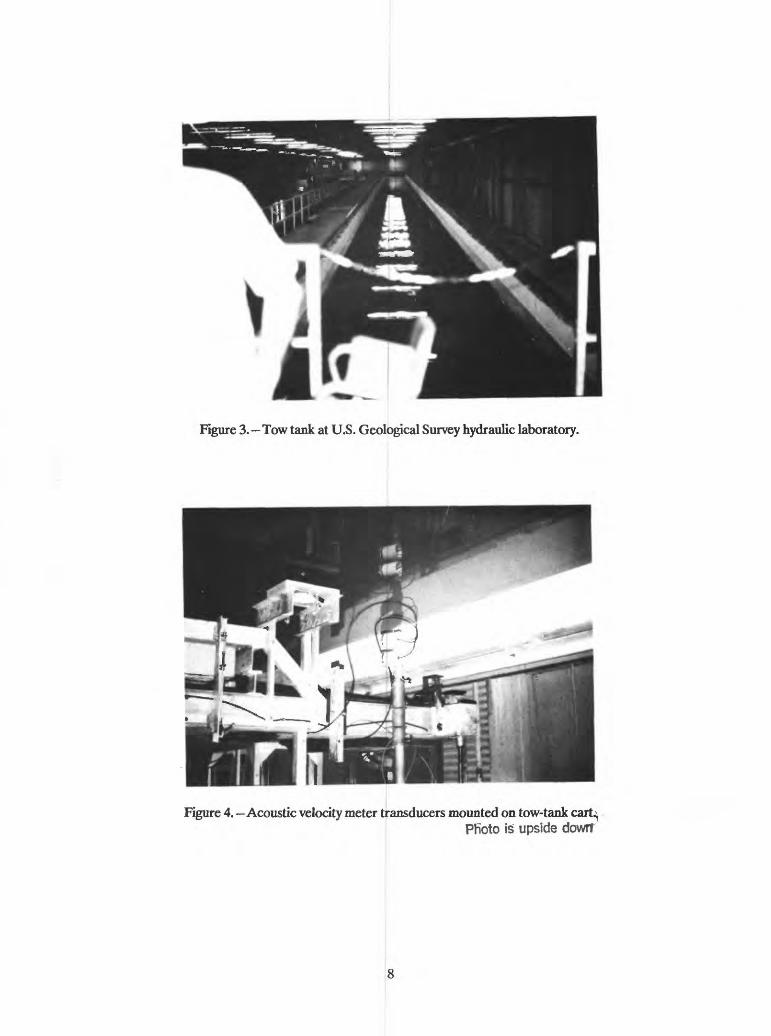
Figure 3. Tow tank at U.S. Geological Survey hydraulic laboratory.

Figure 4. Acoustic velocity meter transducers mounted on tow-tank cart^Pfioto is upside down

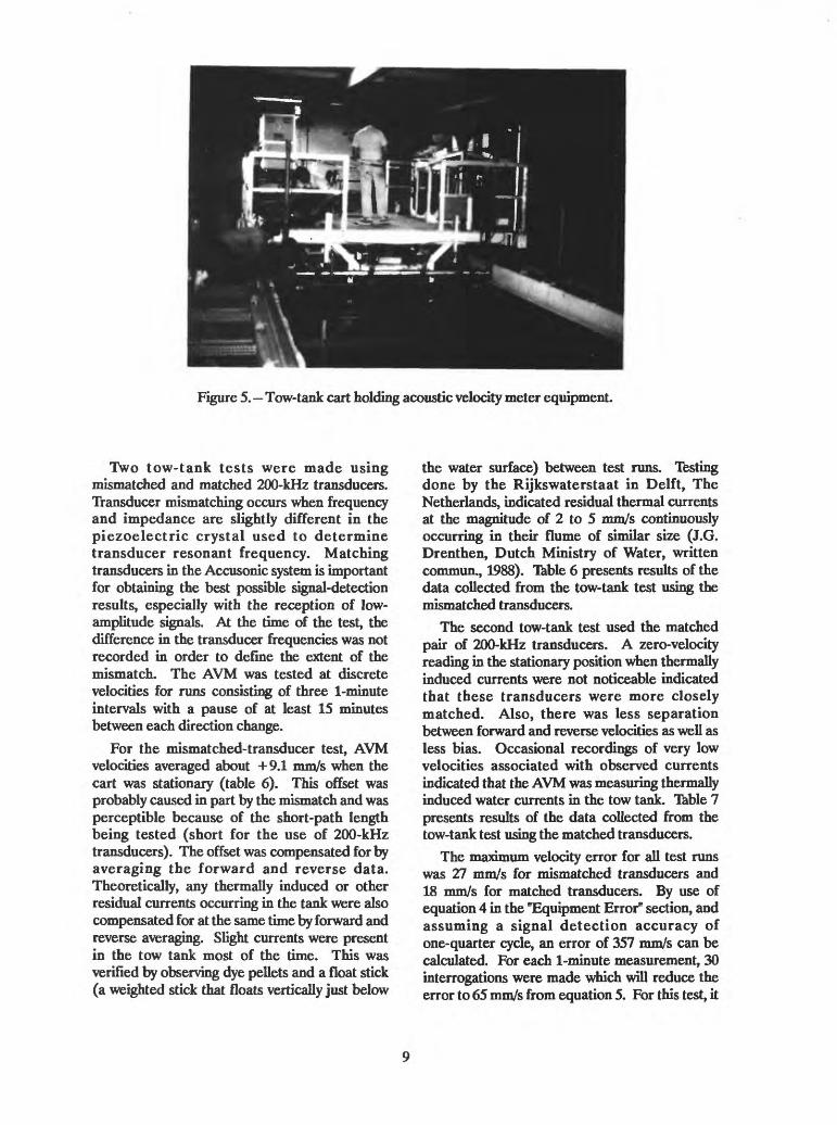
Figure 5. Tow-tank cart holding acoustic velocity meter equipment.

Two tow-tank tests were made using mismatched and matched 200-kHz transducers. Transducer mismatching occurs when frequency and impedance are slightly different in the piezoelectric crystal used to determine transducer resonant frequency. Matching transducers in the Accusonic system is important for obtaining the best possible signal-detection results, especially with the reception of low- amplitude signals. At the time of the test, the difference in the transducer frequencies was not recorded in order to define the extent of the mismatch. The AVM was tested at discrete velocities for runs consisting of three 1-minute intervals with a pause of at least 15 minutes between each direction change.

For the mismatched-transducer test, AVM velocities averaged about +9.1 mm/s when the cart was stationary (table 6). This offset was probably caused in part by the mismatch and was perceptible because of the short-path length being tested (short for the use of 200-kHz transducers). The offset was compensated for by averaging the forward and reverse data. Theoretically, any thermally induced or other residual currents occurring in the tank were also compensated for at the same time by forward and reverse averaging. Slight currents were present in the tow tank most of the time. This was verified by observing dye pellets and a float stick (a weighted stick that floats vertically just below

the water surface) between test runs. Testing done by the Rijkswaterstaat in Delft, The Netherlands, indicated residual thermal currents at the magnitude of 2 to 5 mm/s continuously occurring in their flume of similar size (J.G. Drenthen, Dutch Ministry of Water, written commun., 1988). Table 6 presents results of the data collected from the tow-tank test using the mismatched transducers.

The second tow-tank test used the matched pair of 200-kHz transducers. A zero-velocity reading in the stationary position when thermally induced currents were not noticeable indicated that these transducers were more closely matched. Also, there was less separation between forward and reverse velocities as well as less bias. Occasional recordings of very low velocities associated with observed currents indicated that the AVM was measuring thermally induced water currents in the tow tank. Table 7 presents results of the data collected from the tow-tank test using the matched transducers.

The maximum velocity error for all test runs was 27 mm/s for mismatched transducers and 18 mm/s for matched transducers. By use of equation 4 in the "Equipment Error" section, and assuming a signal detection accuracy of one-quarter cycle, an error of 357 mm/s can be calculated. For each 1-minute measurement, 30 interrogations were made which will reduce the error to 65 mm/s from equation 5. For this test, it

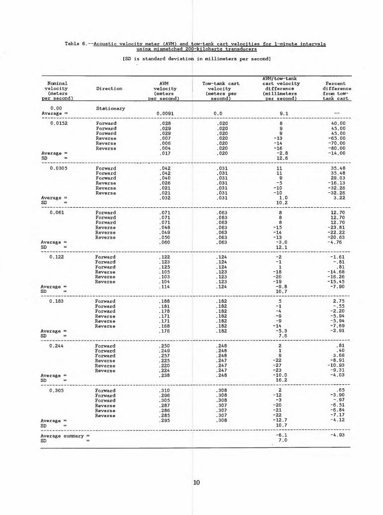
Table 6. Acoustic velocity meter (AVM) and tow-tank cart velocities for 1-minute intervalsusing mismatched 200-kilohertz transducers

[SD is standard deviation in millimeters per second]

Nominalvelocity(meters

per second)

0.00Average =

0.0152

Average =SD

0.0305

Average =SD

0.061

Average =SD

0.122

Average =SD

0.183

Average =SD

0.244

Average =SD

0.305

Average =SD

Average summary =SD

Direction

Stationary

ForwardForwardForwardReverseReverseReverse




ForwardForwardForwardReverseRevers eRevers e



AVMvelocity(meters

per second)

0.0091

.028

.029

.029

.007

.006

.004

.017

.042

.042

.040

.026

.021

.021

.032

.071

.071

.071

.048

.049

.050

.060

.122

.123

.125

.105

.103

.104

.114

.188

.181

.178

.171

.171

.168

.176

.250

.249

.257

.225

.220

.224

.238

.310

.296

.305

.287

.286

.285

.295

Tow-tank cartvelocity(meters persecond)

0.0

.020

.020

.020

.020

.020

.020

.020

.031

.031

.031

.031

.031

.031

.031

.063

.063

.063

.063

.063

.063

.063

.124

.124

.124

.123

.123

.123

.124

.182

.182

.182

.182

.182

.182

.182

.248

.248

.248

.247

.247

.247

.248

.308

.308

.308

.307

.307

.307

.308

AVM/tow-tankcart velocitydifference(millimetersper second)

9.1

899

-13-14-16-2.812.6

11119

-5-10-10

1.010.2

888

-15-14-13-3.012.1

-2-11

-18-20-19-9.810.7

5-1-4-9-9

-14-5.37.6

219

-22-27-23-10.016.2

2-12-3

-20-21-22-12.710.7

-6.17.0

Percentdifferencefrom tow-tank cart

40.0045.0045.00

-65.00-70.00-80.00-14.00

35.4835.4829.03

-16.13-32.26-32.26

3.22

12.7012.7012.70

-23.81-22.22-20.63-4.76

-1.61-.81.81

-14.68-16.26-15.45-7.90

2.75-.55

-2.20-5.94-5.94-7.69-2.91

.81

.403.68

-8.91-10.93-9.31-4.03

.65-3.90-.97

-6.51-6.84-7.17-4.12

-4.93

10

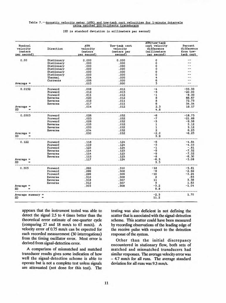
Table 7. Acoustic velocity meter (AVM) and tow-tank cart velocities for 1-minute intervalsusing matched 200-kilohertz transducers

[SD is standard deviation in millimeters per second]

Nominalvelocity(meters

per second)

0.00

Average -

0.0152

Average -SD

0.0305

Average =SD

0.122

Average -SD

0.305

Average =SD

Average summary =SD

Direction

StationaryStationaryStationaryStationaryStationaryStationaryThermalCurrents





AVMvelocity(meters

per second)

0.000.000.000.000.000.000.004.006.005

.008

.012

.011

.020

.019

.017

.014

.026

.025

.029

.033

.033

.034

.030

.118

.119

.123

.114

.114

.115

.117

.292

.299

.299

.310

.318

.312

.305

Tow-tank cartvelocity(meters persecond)

0.000.000.000.000.000.000.000.000.000

.012

.015

.012

.012

.011

.011

.012

.032

.032

.032

.032

.032

.032

.032

.124

.124

.124

.123

.123,123.124

.310

.308

.309

.308

.307

.307

.308

AVM/tow-tankcart velocitydifference(millimetersper second)

000000465

-4-3-18862.34.8

-6-7-3112

-2.03.9

-6-5-1-9-9-8-6.33.5

-18-9

-102

115

-3.29.8

-2.311.2

Percentdifferencefrom tow-tank cart

-33.33-20.00-8.3366.6772.7354.5419.17

-18.75-21.88-9.383.123.126.25-6.25

-4.84-4.03-.81

-7.32-7.32-6.50-5.08

-5.81-2.92-3.24

.653.581.63

-1.04

1.70

appears that the instrument tested was able to detect the signal 2.5 to 4 times better than the theoretical error estimate of one-quarter cycle (comparing 27 and 18 mm/s to 65 mm/s). A velocity error of 0.75 mm/s can be expected for each recorded measurement (30 interrogations) from the timing oscillator error. Most error is derived from signal-detection error.

A comparison of mismatched and matched transducer results gives some indication of how well the signal-detection scheme is able to operate but is not a complete test unless signals are attenuated (not done for this test). The

testing was also deficient in not defining the scatter that is associated with the signal-detection scheme. This scatter could have been measured by recording observations of the leading edge of the receive pulse with respect to the detection response of the system.

Other than the initial discrepancy encountered in stationary flow, both sets of matched and mismatched transducers had similar responses. The average velocity error was - 4.7 mm/s for all runs. The average standard deviation for all runs was 9.3 mm/s.

11

Field Test

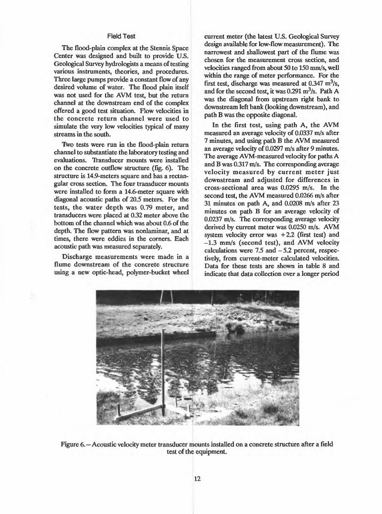
The flood-plain complex at the Stennis Space Center was designed and built to provide U.S. Geological Survey hydrologists a means of testing various instruments, theories, and procedures. Three large pumps provide a constant flow of any desired volume of water. The flood plain itself was not used for the AVM test, but the return channel at the downstream end of the complex offered a good test situation. Flow velocities in the concrete return channel were used to simulate the very low velocities typical of many streams in the south.

Two tests were run in the flood-plain return channel to substantiate the laboratory testing and evaluations. Transducer mounts were installed on the concrete outflow structure (fig. 6). The structure is 14.9-meters square and has a rectan gular cross section. The four transducer mounts were installed to form a 14.6-meter square with diagonal acoustic paths of 20.5 meters. For the tests, the water depth was 0.79 meter, and transducers were placed at 0.32 meter above the bottom of the channel which was about 0.6 of the depth. The flow pattern was nonlaminar, and at times, there were eddies in the corners. Each acoustic path was measured separately.

Discharge measurements were made in a flume downstream of the concrete structure using a new optic-head, polymer-bucket wheel

current meter (the latest U.S. Geological Survey design available for low-flow measurement). The narrowest and shallowest part of the flume was chosen for the measurement cross section, and velocities ranged from about 50 to 150 mm/s, well within the range of meter performance. For the first test, discharge was measured at 0.347 m3/s, and for the second test, it was 0.291 m3/s. Path A was the diagonal from upstream right bank to downstream left bank (looking downstream), and path B was the opposite diagonal.

In the first test, using path A, the AVM measured an average velocity of 0.0337 m/s after 7 minutes, and using path B the AVM measured an average velocity of 0.0297 m/s after 9 minutes. The average AVM-measured velocity for paths A and B was 0.317 m/s. The corresponding average velocity measured by current meter just downstream and adjusted for differences in cross-sectional area was 0.0295 m/s. In the second test, the AVM measured 0.0266 m/s after 31 minutes on path A, and 0.0208 m/s after 23 minutes on path B for an average velocity of 0.0237 m/s. The corresponding average velocity derived by current meter was 0.0250 m/s. AVM system velocity error was +2.2 (first test) and -1.3 mm/s (second test), and AVM velocity calculations were 7.5 and - 5.2 percent, respec tively, from current-meter calculated velocities. Data for these tests are shown in table 8 and indicate that data collection over a longer period

Figure 6. Acoustic velocity meter transducer mounts installed on a concrete structure after a fieldtest of the equipment.

12

Table 8. Acoustic velocity meter (AVM) and current-meter measurement (CMM) velocities in a field testof an acoustic velocity meter system placed in a

[SD is standard deviation in millimeters per second.

AVM velocity CMM velocity Minute (meters per (meters per

1234567

Average

12 3 456789

AverageAS, testSD, test

123456789

1011121314 151617

second) second)

First test, path A

0.037.037.030.033.035.037.027

.0337 0.0295

First test, path B

.029ftOC. UOD.034 m^. Uiji?

.026

.027

.028

.027

.027

.0297 .02951 .0314 .02951

Second test, path A

.025

.027

.026

.027

.028

.030

.024

.027

.030

.026

.024

.022

.027ny*i . \jffj.024.029.030

AVM-CMM velocity difference(millimetersper second)

770357

-3

4.2

-1

4

-4-3-2-3-3

.21.94.0

021235

-1251

-1-320

-145

concrete structure

AS is average summary ]

AVM velocity Minute (meters per

181920212223242Sft <j2677£* t

28293031

Average

12

4567 89

1011121314151617181920212223

AverageAS, testSD, test

second)

Second test,

0.032.026.027.028.028.025.029.023 .026.027 .026.025.027.026

.0266

Second

.026

.027029 . \jfftj.027.024.020.020 .018.018.015.016.017.018.015.018.019.020.023.026.024.024.018.023

.02082 .02422

AVM-CMM CMM velocity velocity (meters per differencesecond) (millimeters

per second)

path A Continued

7123304

-2121021

0.0250 1.6

test, path B

124 2

-1-5-5 -7-7

-10-9-8-7

-10-7-6-5-21

-1-1-7-2

.0250 -3.9

.0250 -.84.2

than tested may reduce differences even more. Data from table 8 also indicate the utility of a second acoustic path crossing at a complemen tary angle to compensate for unknown flow direction. The AVM system indicated many low-amplitude velocity perturbations probably caused by eddies in the very slow moving water.

By increasing the path length of the 200-kHz AVM system from the tow-tank to the field-test configuration, velocity error was substantially decreased. The field tests measured a path length of 20.5 meters, whereas the tow-tank tests

used a path of 4.69 meters. The maximum velocity error for the 20-meter path should be about 16.8 mm/s (based on signal-detection error from table 1 and eq. 5) plus 0.94 mm/s (based on timing oscillator error from table 2 and eq. 5). The test indicated a maximum velocity error of 4.2 mm/s and an overall velocity error, averaged for all the tests, of 1.3 mm/s. The maximum velocity for the 4.69-meter path was 27 mm/s with an average of 4.3 mm/s and can be compared to the longer acoustic path to substantiate the increased accuracy by using a longer acoustic path.

13

SUMMARY AND CONCLUSIONS

Theory has indicated, and tests have shown, that AVM systems can measure very low velocities along the acoustic path with much accuracy, usually within a few millimeters per second. The accuracy of AVM's depends on equipment limitations, the accuracy of acoustic path distance and angle determination, and the stability of the mean velocity to acoustic-path velocity relation.

Equipment limitations depend on the path length and angle, the transducer frequency, the timing oscillator frequency, and the signal-detection scheme. Typically, an acoustic velocity meter using a multiple-voltage threshold signal-detection scheme, 200-kilohertz transducers, and an 80-megahertz timing oscillator and averaging 100 interrogations per minute can have a velocity error of about ±10 mm/s for a 20-meter path length and a velocity error of about ±1 mm/s for a 200-meter path length. Tables used in this report can be used to assess errors from various known equip ment sources; however, for AVM systems that operate with low-signal reception caused by attenuation of the signal in the water or transmis sion lines, signal-detection error can be defined by observations with an oscilloscope.

Error in the measurement of acoustic-path angle or length can result in a proportional measurement bias. Typically, an angle error of1 degree can result in a velocity error of2 percent, and a path-length error of 1 meter in 100 meters will result in an error of 1 percent. In many instances, these measurement errors can be adjusted with check current-meter measure ments. For very low velocity flow where check measurements are impractical, special care must be taken to make the best possible path angle and length determinations.

The accuracy of mean velocity determination, which is related to the water environment, can be more difficult to assess because it relies on the stability of the vertical velocity distribution and the existence of density gradients in the stream. Tables included in this report can help to assess error caused by the various known or predicted environmental sources. Ray bending (signal refraction) depends on path length and density gradients present in the stream. Any deviations from a straight acoustic path between transducers can change the unique relation between path velocity and mean velocity. These deviations can then introduce error hi the mean velocity computation. In many short-path situations (less than 200 meters), this error can be avoided, or is of minimal importance. Typically, for a 200-meter path, the resultant error is less than 1 percent, but for a 1,000-meter path the error can be greater than 10 percent.

Recent laboratory and field tests at the U.S. Geological Survey hydraulic laboratory facility at the Stennis Space Center hi Mississippi have substantiated assumptions of equipment limitations. Tests yielded velocity errors less than values predicted from the error sources covered in this report. However, the tests were not as extensive as they might have been. The signal-detection scheme was not tested under conditions of signal attenuation, and mean- velocity to path-velocity relations were not tested under conditions of changed vertical density gradients. An Accusonic model 7410 AVM manufactured by Ferranti, Ocean Research Equipment, Inc., was tested in both tow-tank and field installations. Tow-tank tests, based on the use of an AVM with a 4.69-meter path, had a maximum velocity error of 27 mm/s, and an average standard deviation of 9 mm/s; and the field tests, based on the use of an AVM with a 203-meter path, had a maximum velocity error of 8 mm/s and an average standard deviation of4 mm/s

14

REFERENCES CITED

Chow, V.T., editor-in-chief, 1964, Handbook of applied hydrology: New York, McGraw-Hill Book Company, sec. 1-29, p. 1-1 to 29-30.

Clay, C.S., and Medwin, Herman, 1977, Acousti cal oceanography, principles and applica tions: New York, John WUey, 544 p.

International Organization for Standardization, 1985a, International Standard 6416, Liquid flow measurement in open channels- measurement of discharge by the ultrasonic (acoustic) method: Switzerland, Interna tional Organization for Standardization, 20 p.

- - - 1985b, International Standard 6418, Liquid flow measurement in open channels -

ultrasonic (acoustic) velocity meters: Switzerland, International Organization for Standardization, 13 p.

Laenen, Antonius, 1983, Measuring water surface and stream bed elevation changes with the acoustic velocity metering system: Water Resources Research, v. 19, no. 5, October 1983, p. 1317-1322.

1985, Acoustic velocity meter systems: U.S. Geological Survey Techniques of Water Resources Investigations, book 3, chap. A17, 38 p.

Laenen, Antonius, and Smith, Winchell, 1983, Acoustic systems for the measurement of streamflow: U.S. Geological Survey Water- Supply Paper 2213,26 p.

*U.S.GOVERNMENTPRINnNGOFFICE: 198 9 -$31 "169/ 00002

15

accuracy of acoustic velocity metering systems for measurement of

Documents