Power Systems Engineering Research Center

ACCURACY IMPROVEMENT STRATEGIES FOR

PROBLEMATIC POWER SYSTEM

MEASUREMENTS AND THEIR EFFECT ON STATE

ESTIMATION

A Supplementary Project Report for Project S-22

Brian C. Mann G. T. Heydt

Arizona State University

PSERC Publication 06-XX

July 2006

Information about this project For information about this project contact: Gerald T. Heydt, Ph.D. Arizona State University Department of Electrical Engineering Tempe, AZ 85287 Tel: 480-965-8307 Fax: 480-965-0745 Email: heydt@asu.edu

Power Systems Engineering Research Center

This is a project report from the Power Systems Engineer-ing Research Center (PSERC). PSERC is a multi-university Center conducting research on challenges facing a restruc-turing electric power industry and educating the next gen-eration of power engineers. More information about PSERC can be found at the Center’s website: http://www.pserc.org.

For additional information, contact:

Power Systems Engineering Research Center

Arizona State University

P. O. Box 875706

Tempe, AZ 85287-5706

Notice Concerning Copyright Material

PSERC members are given permission to copy without fee all or part of this publication for internal use if appropriate attribution is given to this document as the source material. This report is available for downloading from the PSERC website.

©2005 Arizona State University. All rights reserved.

iii

Executive Summary

This research discuses several power system measurement pre-processing tech-

niques, which may improve calculations like state estimation (SE). SE is a proven tech-

nology, but operates under assumptions which may be inappropriate. The concept of

non-collocated power measurement error is introduced, where reactance between current

and voltage instruments creates power calculation error. A calculation-based method for

correcting these measurements is presented and shown to slightly improve state esti-

mates. SE may assume balanced operation. However, unbalance is common in power

systems. Under certain assumptions, single-phase power measurements and complex

current unbalance factor (CCUF) can calculate three-phase power. This yields better

measurements, but is shown to have little effect improving traditional SE. Methods for

estimating or calculating CCUF are also presented. SE often assumes all measurements

are simultaneous. A simple linear prediction method used to identify late measurements

is studied and shown to work in systems with low measurement noise and low system

dynamics.

The main elements of this research are:

• It is possible to correct the measurement error associated with reactance in-

between the CT and PT component of a power measurement from knowing the

non-collocated power measurement, a local voltage magnitude, and the reactance.

This is a software solution that avoids hardware reinstallation and may have a

positive effect of state estimation results by lowering estimate error and, more

iv

dramatically, lowering state estimate variance. The practical significance of this

is that a software patch can be used to correct for non-collocated power measure-

ments, thereby avoiding a hardware fix.

• State estimators that incorporate three-phase power flow may operate under a bal-

anced system assumption when unbalanced conditions. A more accurate three-

phase power calculation may be calculated from single-phase measurements and

the complex current unbalance factor, resulting in improved state estimation out-

put. Methods for estimating or directly calculating the complex current unbalance

factor are also presented. The practical significance of this is that through a soft-

ware correction procedure, at least under some circumstances, it may be possible

to correct for unbalanced measurements.

• A linear signal prediction algorithm is presented which may have a positive effect

on power system state estimation in the presence of measurement latency. The

presented algorithm has the advantage of being less complex than existing de-

layed measurement correcting algorithms presented in the literature. The value of

this technical topic is that latency can be compensated through a software patch,

and at least three methods are described in this report.

v

ACKNOWLEDGEMENTS

The authors thank the generous support of the Power Systems Engineering Re-

search Center, and the support of the Salt River Project (SRP) for this project. In particu-

lar, the following investigators at SRP are acknowledged for their support and expertise:

G. Strickler, N. Logic, S. Sturgill, J. Singh.

The authors also thank Dr. Daniel J. Tylavsky and Dr. Vijay Vittal for their tech-

nical input. The authors acknowledge the technical contributions of Ms. Lida Jauregui –

Rivera. Thanks is also due for Professor Richard G. Farmer, whose valuable experience

and helpfulness played a role in the first part of this research. Useful comments of L. Jer-

riel were used in the project and we acknowledge Mr. Jerriel’s input.

vi

TABLE OF CONTENTS

Page

TABLE OF FIGURES..................................................................................................... viii

TABLE OF TABLES ........................................................................................................ ix

NOMENCLATURE .......................................................................................................... xi

CHAPTER 1 STATE ESTIMATION........................................................................... 1

1.1 State estimation: an introduction ................................................................ 1 1.2 The theory of state estimation..................................................................... 2 1.3 Objectives ................................................................................................... 5 1.4 Literature review......................................................................................... 5 1.5 Organization of this thesis ........................................................................ 13

CHAPTER 2 NON-COLLOCATED POWER MEASUREMENT CORRECTION..................................................................................................... 15

2.1 Non-collocated measurements .................................................................. 15 2.2 Illustrative examples ................................................................................. 24 2.3 Observations drawn from the example ..................................................... 31

CHAPTER 3 UNBALANCE FACTOR USE FOR SINGLE PHASE STATE ESTIMATION IMPROVEMENT........................................................................ 34

3.1 Complex voltage and current unbalance factor ........................................ 34 3.2 Test cases for observing the effect of the Equation (3.5) adjustment on

state estimation.......................................................................................... 39 3.3 Observations drawn from test cases.......................................................... 47 3.4 Notes on calculating complex unbalance factor without phasor

measurements............................................................................................ 49 3.5 Summary of results ................................................................................... 58

CHAPTER 4 LINEAR PREDICTION METHODS FOR NON-SIMULTANEOUS MEASUREMENT CORRECTION TO IMPROVE STATE ESTIMATION ..... 60

4.1 Non-simultaneous measurements ............................................................. 60 4.2 Linear measurement prediction................................................................. 61 4.3 Test case to find optimal linear prediction method................................... 66

CHAPTER 5 CONCLUSIONS AND RECOMMENDATIONS ............................... 72

5.1 Conclusions............................................................................................... 72 5.2 Recommendations..................................................................................... 73

vii

Page

REFERENCES ................................................................................................................. 74

APPENDIX A DESCRIPTION OF THE TEST CASES................................................ 79

APPENDIX B SAMPLE MATLAB CODE.................................................................... 81

viii

TABLE OF FIGURES Page

Figure 1.1 Pictorial of a recursive method for nonlinear state estimation ..........................4

Figure 1.2 Pictorial of a state estimator ...............................................................................7

Figure 1.3 A flowchart illustrating the discrete Kalman filter loop...................................13

Figure 2.1 An example of a complex power measurement setup ......................................16

Figure 2.2 A model for the reactance between CT and PT in a non-collocated

measurement ..........................................................................................................17

Figure 2.3 An example of a non-collocated power measurement instrument placing.......17

Figure 2.4 A circuit diagram showing how the V2, S21 case is similar to Case A..............21

Figure 2.5 A new notation for the non-collocated impedance model for use in Case B ...21

Figure 2.6 An 11 bus test bed inspired by the 500 kV lines of the US southwest.............27

Figure 3.1 The three-bus test bed topology used in Cases 5-8 ..........................................40

Figure 3.2 Three-phase current phasors that sum to zero ..................................................54

Figure 3.3 Right triangle from angle α and law of cosines relationship............................55

Figure 4.1 The linear measurement prediction model algorithm.......................................62

Figure 4.2 An example of a randomly delayed measurement signal .................................65

Figure 4.3 An example of the randomly delayed measurements effect on the linear

prediction algorithm, from Test Case 9a................................................................66

Figure 4.4 The five bus test bed for Cases 9-14 ................................................................68

ix

TABLE OF TABLES Page

Table 2.1 A parameter replacement guide to use Case A with S21 and V2 known or Case B

with S12 and V2 .......................................................................................................21

Table 2.2 Line reactance for the Case 0-4, 11-bus test bed, on a 100 MVA, 500 kV base25

Table 2.3 Test bed reactive values for testing non-collocated measurements in Cases 1-4,

relative to circuit in Figure 2.1, on a 100 MVA and 500 kV base.........................29

Table 2.4 State estimation Cases 0-4 testing criteria used with the 11 bus test bed..........30

Table 2.5 Test bed average δ after 1000 runs compared to actual δ, for Cases 0-4...........30

Table 2.6 Test bed average |V| after 1000 runs compared to actual |V|, for Cases 0-4 ......30

Table 2.7 Test bed average P measurement after 1000 runs compared to actual P, for

Cases 0-4................................................................................................................31

Table 2.8 Test bed average Q measurement after 1000 runs compared to actual Q, for

Cases 0-4................................................................................................................31

Table 3.1 Assigned line-to-neutral base case voltage values for Cases 5-8 ......................41

Table 3.2 Line reactance values for three-phase test bed used in Cases 5-8 .....................42

Table 3.3 Resulting base case current values for the three-bus test bed used in Cases 5-842

Table 3.4 Three-phase test bed exact power measurements in Cases 5-8 .........................42

Table 3.5 Key to identify test case names..........................................................................47

Table 3.6 The 2-norm residuals of the difference between test states from case 5-8 and

the base case states from Table 3.4 values.............................................................47

x

Page

Table 3.7 The 2-norm of the residuals between raw state estimates from Cases 5-8 and

base case estimates from Table 3.4 values.............................................................47

Table 3.8 Normalized state estimate residuals from the three-phase test bed utilizing the

two-magnitude, estimated UI method, using Cases 5-8 system data .....................52

Table 3.9 Normalized state estimate residuals from the three-phase test bed utilizing the

three-magnitude, estimated UI method, using Cases 5-8 system data ...................53

Table 4.1 Identities of test Case 9-14.................................................................................69

Table 4.2 Results for test Cases 9-14.................................................................................70

Table A.1 Guide to the test case denomination and meaning............................................80

xi

NOMENCLATURE a A complex phasor °−∠ 1201 and a real number which is a magnitude

of a bus voltage V1 A Matrix that linearly relates past measurements to future measurements AC Alternating current A/D Analog/digital ARMA Mixed auto-regressive moving average b A variable which is the real component of the current through line

reactance X1 c A variable which is the imaginary component of a current through

line reactance X1 CT Current transformer CUF Current unbalance factor d A variable which is the real component of a mid-line voltage Vx δa Voltage phase angle of bus a e A variable which is the imaginary component of a mid-line voltage Vx EMS Energy management systems f A variable which is the real component of a current through line reac-

tance X2 g A variable which is the imaginary component of a current through

line reactance X2 GPS Global positioning system h A variable which is the real voltage of a bus voltage V2 H State estimation coefficient matrix i Counter index I+ Positive sequence current I- Negative sequence current I0 Zero sequence current Iab Current between buses a and b Ia, b, c Current for phase a, b, or c IEEE Institute of Electrical and Electronics Engineers j Complex number 1− J(x) Jacobian matrix k A variable which is the imaginary component of bun voltage V2 or a

time step variable in the discrete Kalman filter algorithm K The Kalman gain, in the discrete Kalman filter M Measurement-to-branch matrix and symmetrical component transfor-

mation index Nm Number of measurements Ns Number of states P Active power and the error covariance matrix in the discrete Kalman

filter PMU Phasor measurement unit PT Potential transformer p.u. Per-unit

xii

Q Reactive power and the expected value of noise w2 in the discrete Kalman filter

R Covariance matrix of measurement errors, weighting matrix S Complex power S3φ Three-phase complex power Sab Complex power calculated from Va and Ib SE State estimation t Time in seconds UI Current unbalance factor UV Voltage unbalance factor UTC Coordinated Universal Time v Measurement error in discrete Kalman filter algorithm V Voltage (rms phasor) V1+, 2+ Positive sequence voltage for bus 1 or 2 V+ Positive sequence voltage V- Negative sequence voltage V0 Zero sequence voltage Va, b, c Voltage for phase a, b, or c |V|a Voltage magnitude of bus a or point a VUF Voltage unbalance factor w White noise associated with a measurement W Residual sensitivity matrix WLS Weighted least squares x Vector of state values X Reactance z Vector of measurements η Measurement error φ Matrix which relates xk to xk+1 in the discrete Kalman Filter

1

CHAPTER 1 STATE ESTIMATION

1.1 State estimation: an introduction

State estimation (SE) is a mathematical process in which physical measurements

and physical models are combined in an optimal way. That is, measurements taken in the

field are used with models and the states of the system (in the power engineering applica-

tion, the states are typically the bus voltage phase angles and magnitudes) are selected or

calculated such that the states match the measurements in some best way. The usual SE

technique utilizes what is known as the least squareserror algorithm. In this algorithm,

the system model is linearized as

z = Hx,

where z is a vector of measurements, x is the system states (a vector), and H is the rela-

tionship between the measurements and the states. The matrix H is also known as the

process matrix. If z is an m-vector, and x is an n-vector, then H is an m by n rectangular

matrix. Typically,

m >> n.

The SE process is the minimization of |Hx – z|. In the least squares algorithm, the norm

indicated is a Euclidean norm. In essence, the SE algorithm causes x to be selected such

that |Hx – z| is minimized. The notation x (read ‘x – hat’) is the estimate of the state vec-

tor x at this minimum. The vector

H x – z = R

2

is called the residual vector, and the Euclidean norm,

|H x – z|2 = r

is the residual magnitude.

The SE solution involves taking the pseudoinverse of the process matrix H de-

noted as H+. The optimal x, that is the best estimate of x, is

.ˆ zHx +=

In this proposed work, the residual vector R and the residual magnitude r shall be

examined with respect to errors in measurements z and errors in the process model H.

The concept is to not only identify where the errors arise, but also identify ways to cor-

rect the errors.

References [6, 17, 36-38] document state estimation as applied to power engineer-

ing, and errors in the state estimation process.

1.2 The theory of state estimation

State estimation is an increasingly common part of power utility energy management

systems (EMSs). State estimation is a mathematical tool that is used to calculate voltage

magnitude, phase angles, and other AC system variables from system measurements,

such as complex power. State estimation is a software tool that relies on:

• Input data (measurements)

• Fundamental AC circuit laws

• The system model.

State estimation modules in EMSs are a proven technology that relies on redundancy of

measurements, self-identification of problematic conditions, and bad data rejecting.

3

However, some state estimation accuracy affecting conditions have been known to exist,

including: system blind spots, miscalibrated instruments, measurement error or bias,

power system model errors, communication delay, communication channel bandwidth

limits, and analog/digital (A/D) conversion resolution. If conditions exist that may affect

state estimation accuracy, then it is important to characterize them for possible mitiga-

tion.

The most common state estimation method implemented by power utilities today

is the weighted least squares (WLS) method, which is detailed in [17]. In essence, the

WLS method is based on physical models for active and reactive power (P and Q).

Measurements of P and Q are “forced” equal to calculated values from the physical

model. The difference between the measurements and the model is called the residual.

The residual is minimized in the least squares sense. The WLS has the ability to “flag”

large measurement errors and, as an iterative process, may take more time to converge

when error is present. However, some sources of error are small enough to escape notice

and can lead to a persistent source of estimate accuracy degradation. Perhaps the greatest

danger of error in state estimator input data relates to convergence. Figure 1.1 shows the

generalized concept of nonlinear state estimation as applied in power engineering. The

figure shows an iterative method for solving the nonlinear state estimation problem

through recursive linearization. If the number of linearizations becomes large, it is as-

sumed that the process is nonconvergent. If the input data has excessive error, the pros-

pect of nonconvergence becomes a concern.

4

Figure 1.1 Pictorial of a recursive method for nonlinear state estimation Another difficulty associated with state estimation is that SE, along with some

other EMS calculations, traditionally utilizes a single-phase model to represent a multi-

phase power system [29]. The single-phase power system model works well under sym-

metrical and balanced conditions. In the balanced instance, the negative and zero se-

quence currents and voltages are zero. This single-phase system can even produce ac-

ceptable answers when unbalance exists between the phases, providing zero and negative

sequences are sufficiently small [12, 13]. However, unbalance between the three phases

of a power system is the norm rather than the exception, for instance due to non-

transposed transmission lines, single phase loads, or unbalanced loads [29]. These phe-

nomena can lead to long convergence times, non-convergence, or inaccurate results in

state estimation, if the unbalance is sufficiently severe.

State estimation can play a crucial part in the day-to-day operation of a power sys-

tem utility. The system measurements are used for real-time operations like optimal

power flow calculations. Proper system operation with regard to avoidance of insecure

5

conditions includes situational awareness; therefore the state estimator plays an impor-

tant role in power system security. The importance of state estimators with regard to

blackout avoidance is documented in [14]. A further motivation: in the increasingly de-

regulated power environment in the United States and abroad, more economic operation

means savings for customers and power providers alike. Economic benefits might be re-

alized if operators have a more accurate situational awareness of the system through im-

proved state estimation.

1.3 Objectives The main objective of this research is to identify some potential problems associ-

ated with common state estimation methods and to design “software fixes” or other solu-

tions to these problems. The methods to improve state estimation and power system

monitoring include:

• Accounting for measurements due to voltage and current instruments that are not col-

located.

• Using unbalance factor values to improve model accuracy for power systems with

three-phase measurements.

• Estimating measurement values in a system with non-simultaneous measurements.

1.4 Literature review

Power system state estimation is a documented subject that occupies a very large vol-

ume of technical literature. Classic papers on the subject include Schweppe’s original

paper on the subject and the paper that introduced Kalman filters [2], [3]. The method of

6

weighted least squares state estimation (WLS) is important because it is the method most

implemented by power utilities today. Many state estimation textbooks go over the algo-

rithm in detail, including reference [17]. The process will be outlined briefly later in

this section.

There are many papers that concern measurement error and topology error identifica-

tion in state estimation, particularly the weighted least square case. The error flagging

and state identification properties of WLS SE make topology identification possible. One

paper discusses comparing line measurements to well-observed adjacent measurements

for spotting and correcting model parameter errors [4]. Another discusses using artificial

neural networks to analyze unfiltered state estimation data for identifying and correcting

topological and analytical errors [5]. Another paper that deals with finding topology er-

rors is [6], where a residual sensitivity matrix W is compared to a measurement-to-branch

matrix M. The idea behind this method is that single topology errors will have state esti-

mation residuals that stand out from the rest of the system. The limitations of this system

are discussed, as well as its application to real systems with possibly more than one to-

pology error. The paper [7] is less general and discusses finding topology errors in power

system state estimation by correlating measurements from suspected trouble-spots to

those of known system anomalies, but only for single and multiple bus-split topology er-

rors. The paper [8] presents an effective method for estimating a power networks topol-

ogy in the presence of bad data and topology errors. This method tests measured real and

reactive power flows with the WLS, but utilizing the Huber M-estimator method. In [9],

the use of state-estimation for identifying topology errors is discussed in the instance of

line or transformer outage, bus split and shunt capacitor/reactor switching.

7

The WLS method is a common type of state estimation and has been realized mathe-

matically for single-phase and multi-phase power systems. The general WLS method

contains a measurement vector z, a state vector x, a matrix H containing the coefficients

that relate z and x, as well as the covariance matrix of measurement errors R. Figure 1.2

is a simple pictorial of the concept. The residual between the measured and estimated

states is minimized iteratively by the following relationship,

]][][[]][min[)(min 1 xHzRxHzxJ T −−= − .

In typical single-phase power system usage, the measurements will be real and reactive

power and the states will be bus voltages magnitudes and phase angles.

Figure 1.2 Pictorial of a state estimator

Examples of detailed three-phase least squares state estimation algorithms exist in the

literature. There is a paper goes into detail on the modeling of many three-phase power

system components and discusses a three-phase state estimation method similar to WLS

[11]. Also discussed are the technologies available which make three-phase state estima-

tion possible. A test bed is presented in reference [12] that shows the effect of measure-

8

ment noise on state estimation accuracy, with the conclusion that noise two times larger

the meter accuracy has a profound effect against satisfactory measurement readings.

Unbalanced systems conditions occurring in three-phase state estimation have also

been studied in the literature. A number of power systems are traditionally modeled in

single-phase by utilizing the positive sequence components from three-phase measure-

ments, even if a degree of unbalance is present. The paper [13] studies the error that oc-

curs when a three-phase power system uses a single-phase model under unbalance condi-

tions. The study uses an IEEE 30 bus system for a test model, where non-transposed

lines or unbalanced loads are introduced with differing severity. Also present is random

error in the systems power measurements. The result in each non-transposed lines case

was bias in the final state estimation results and that modeling errors were not flagged by

the state estimator. In the case of unbalanced loads with transposed lines, the error in the

state estimation results were more severe. A 10% unbalance in one phase current re-

sulted in skewed data similar to the worst non-transposed line case studied in this paper

and the more unbalanced cased errors to increase significantly. While all of the non-

transposed and unbalanced conditions resulted in a mismatch compared to “perfect”

measurements, only the most extreme tested case of load unbalance was flagged as bad

data by the state estimator.

This thesis presents the use of the unbalance factor to improve state estimation. Un-

balance factor is calculated from the negative and positive components of voltage or cur-

rent resulting from symmetrical transformation, where UI is the current unbalance factor

(CUF) and UV is the voltage unbalance factor (VUF). The unbalance factor was first

proposed as a ratio between the amplitudes of the negative and positive sequence voltage

9

or current [32], but has seen much more use lately as a complex ratio. The exact unbal-

ance factor calculations are,

+

−=IIU I and

+

−=VVUV .

There is very little in the literature about using unbalance factor values in state estima-

tion. Unbalance factor is mainly used to quantify unbalance in a power system. Voltage

unbalance factor is more often studied than current unbalance factor. The line-to-line

voltage phasors always form a closed triangle and use of geometry and phasor mathemat-

ics can easily yield voltage complex unbalance factor, whereas current complex unbal-

ance factor. Methods for calculating complex voltage unbalance factor from line-to-line

voltage magnitudes are shown in [18], while line-to-neutral voltage magnitudes are

shown to have calculable voltage angles in the absence of a zero-sequence component in

reference [32]. Another paper details traditional methods used by utilities to measure un-

balance factor and how this can be improved and used to represent line loss during unbal-

anced system conditions [19]. The reference [19] also mentions that the greatest cause of

phase unbalance in a power system is single phase loads, such as AC railways or fur-

naces. Use of unbalance factor to describe the effects of these single-phase loads is

documented in the literature, for instance a paper that discusses using unbalance factor to

characterize the unbalance that can affect a single-phase load induction motor [20]. De-

spite all of these uses for complex unbalance factor, it is not a commonly metered quan-

tity and requires special equipment or techniques.

Another potential problem facing state estimation is measurement timing. The

state estimation algorithm depends on measurement inputs from throughout the system.

If the states at time t=0 are to be calculated, for example, then the measurements must

10

also be from time t=0, because old measurements may not accurately reflect the dynamic

power system. Potential problems occur with this since power systems are often large

entities, especially if you take into account separate, but interconnected, power systems.

The communication system in this power system can sometimes report measurements

from outlying instruments later than others [22]. The late measurement may be signifi-

cantly late such that calculations like SE use a mix of new measurements and delayed

measurements. Most SE algorithms assume no measurements are delayed, therefore er-

ror from the delayed measurements will be perceived as measurement error. Very com-

plete state estimation models also take into account other interconnected power systems.

Relying on the interconnected utility or a central power pool for measurements or state

information may also add a time skew [23]. When collecting measurements for a state

estimation calculation some of the measurements may be anywhere from 10 seconds to

60 minutes late (especially if waiting for state estimation results from a separate but in-

terconnected power system) [23]. Suspected late measurements can be discarded from

the SE, but this may result in poor performance [23]. It may be better to filter the sus-

pected late measurements and some filtering methods will be discussed later in this sec-

tion.

Measurement timing has seen much improvement in the past two decades. The

Department of Defense’s Global Positioning System (GPS) system is series of 24 satel-

lites which can provide a time signal to an earthbound antenna that is accurate within 200

ns of Coordinated Universal Time (UTC) [10, 24]. Many power utilities are also having

their proprietary measurement communication systems synchronized with GPS [25]. The

GPS system is also an integral part of the PMU device and the GPS signal is the only re-

11

gional time source accurate enough to meet IEEE standards for real-time phasor meas-

urements [24]. PMU devices measure voltage and current in three phases and return

positive sequence phasor values, as well as time stamps for each measurement. This

seems to offer a solution to time skew problems, since measurements could have their

time stamps compared to see if any of them are “late”, but that would require a signifi-

cant amount of PMU coverage in a power system. However, most power systems have

few PMUs, if any at all. Many studies have been done concerning the optimal placement

of PMUs, such that total power system coverage is accomplished with a minimum of

PMU units [26] and [27]. Were this implemented, time stamp solutions would be viable

to the delayed measurement problem. PMU usage may see an increase in the future,

since at least one protective relaying manufacturer (SEL, Pullman WA) now offers a

PMU signal in most of its new relays. There is, nonetheless, a cost of communicating the

PMU signal and integrating that signal into the software tools. Besides unit cost and time

stamping, PMUs also seem to offer an advantage of additional measurements for the state

estimation equation: phasor angles. However, the addition of phase angles to the meas-

urement vector of WLS SE only increases SE confidence when the phase angle meas-

urements are very accurate (δError ≤ 0.1˚) [28].

PMUs use may not offer a practical solution to measurement time skew, but sev-

eral computational algorithms exist to improve measurement data with time skew. Many

studies have been done using Kalman filter algorithms to improve time skewed meas-

urement data [23], [29]. The Kalman filter is a time-tested algorithm that can be used to

account for noisy measurements when calculating states (and adopted to account for

12

measurement delay). Discrete Kalman filtering assumes the measurement signal can be

estimated and the state calculated by the following equations,

kkkk

kkxx

vxHzwxx

+=+=+ φ1 .

In the previous equations, k is the time, x is the measurement vector, φ relates xk to xk+1

(often the state transition matrix), and w is an assumed white noise component with

known covariance structure. The state transition equations, with measurement vector z

and coefficient matrix H, is familiar from WLS SE methods and this time includes a vec-

tor of measurement error v (white noise with known covariance structure and not coupled

with w). The discrete Kalman filter loop is shown in Figure 1.3, where K is the Kalman

gain, P is the error covariance matrix, Q is the expected value of noise w when squared,

and R is the expected value of noise v when squared. A more detailed explanation of the

Kalman filtering method can be found in [34]. The Kalman filter algorithm is often used

to sort out measurement noise, and therefore has to be changed somewhat to handle de-

layed measurements. The literature presents a method for Kalman filtering against delays

of a single sampling period that occur randomly with known probability [23] and times

when the exact delay of each measurement is known [35].

Also present in the literature are algorithms less common than the Kalman filter

used to account for delayed measurements. Presented in [22] are Winter’s Multiplicative

Seasonal Model and The Mixed Autoregressive-moving Average (ARMA). The Win-

ter’s Multiplicative Seasonal Model has three smoothing components, controlling the pre-

dicted mean, predicted slope, and a seasonal factor.

13

Figure 1.3 A flowchart illustrating the discrete Kalman filter loop

1.5 Organization of this thesis

This thesis is organized into five chapters:

1. State estimation introduction and literature review

2. Description and solution of the problem of non-collocated measurements for

SEs.

3. Effects of voltage and current unbalance conditions on SE.

4. State estimation utilizing unsynchronized signals.

5. Conclusions and recommendations.

Compute Kalman gain: ( ) 1−−− += k

Tkkk

Tkk RHPHHPK

Update estimate with measurement zk:

⎟⎠⎞

⎜⎝⎛ −+= −−

kkkkkk xHzKxx^^^

Compute error covariance for updated estimate:

( ) −−= kkkk PHKIP

Project ahead:

kkk xx^

1

^φ=−

+

kT

kkkk QPP +=− φφ

Enter prior estimate −kx

^ and

Its error covariance −kP

14

In addition, two appendices document the thesis. This is:

A: Guide to test case denomination and meaning.

B: Samples of MATLAB code used in this research.

15

CHAPTER 2 NON-COLLOCATED POWER MEASUREMENT CORRECTION

2.1 Non-collocated measurements

Complex power is a function of the complex voltage and current, where S=VI*.

Power measurement devices operate by sampling the voltage, v(t), and the current, i(t),

which are converted to a digital signal by an A/D converter. The digital current and volt-

age signals are processed to obtain a product utilizing a power transducer. In the vast

number of SE applications, the digital output of the power transducers is passed to a cen-

tral computer via the Supervisory Control and Data Acquisition (SCADA) system. The

power transducers send signals every ∆t seconds where ∆t is typically in the 1 to 5 second

range. The SCADA system has been designed to accommodate the power transducer

signals in addition to the many other signals passed through this data acquisition hard-

ware. Also, voltage magnitude and current magnitude signals may be obtained from A/D

transducers, and, again, passed to the central computer via the SCADA system. In recent

years, a new device has been augmented into the traditional system described: this is the

phasor measurement unit. A PMU is capable of calculating the phase of voltage and cur-

rent measurements, and these signals are available at relatively high sample rates (e.g., 1

second). At the time of writing, few electric utility companies have installed PMUs.

However, there is a clear trend and thrust to radically increase the number of PMUs in

power systems. Because PMUs are GPS based devices, they are capable of time stamp-

ing measurements. Because phase angles of V and I are available in PMUs, complex

power P+jQ may be readily calculated. An example of a power measurement instrument

setup is shown in Figure 2.1. In this figure, a PMU is shown. In the large majority of

16

power systems, PMUs are not used: in these cases, P and Q measurements are simply

passed to the SCADA system. When measuring or calculating complex power, the volt-

age and current must be taken from the same place in the system. In the case of a non-

collocated power measurement, this is not the case. The impedance between the CT and

PT can be represented as the circuit shown in Figure 2.2. In the case of a non-collocated

measurement it is assumed that the instruments are not far apart and well within the range

of typical short line modeling limits. Because the CT and PT are often not separated by

even a kilometer, resistance in the impedance model has been assumed to be negligible.

An example of a non-collocated instrument placement is shown in Figure 2.3.

Figure 2.1 An example of a complex power measurement setup taken from [1]

When discussing power values in this paper, the notation Sab will be used. The

subscript a will be the same subscript as the voltage used to calculate Sab and the sub-

script b will be the subscript of the current used to calculate Sab. For instance, meaningful

power values from the system in Figure 2.2 would be S11 and S22, which are calculated as

follows,

17

*1111 IVS =

*2222 IVS = .

Figure 2.2 A model for the reactance between CT and PT in a non-collocated measure-ment

Figure 2.3 An example of a non-collocated power measurement instrument placing

Note that in the S11 and S22 expressions, the notation V, I, and S are complex num-

bers (i.e., sinusoidal steady state, phasor, analysis). The notation | · | shall be used to de-

note amplitude. Examples of non-collocated power measurements from the system in

Figure 2.2 would be S12 (shown with instrument placing in Figure 2.3) or S21. Each of

these is calculated as follows,

*2112 IVS =

*1221 IVS = .

18

Complex power calculations can be put into a general matrix form, where V is a

vector of complex voltage values at a bus (sinusoidal steady state, phasor notation) and

similarly, let I be a vector of line currents. The dimensions of these vectors are NV and

NI, respectively. Further, there is a complex power matrix of dimension NV by NI defined

as

HVIS = .

where (·)H denotes the hermitian operation (complex conjugate followed by a transpose).

Then elements of matrix S in positions like Saa represent the familiar conventional com-

plex power. However, elements like Sab, a ≠ b, represent non-collocated signals that are

dimensionally like P + jQ, but do not represent conventional active and reactive power.

The issue is the ‘correction’ of non-collocated terms like Sab to obtain conventional active

and reactive power like Saa. Consider the case that NV = NI = 2, and the current vector I is

written with polarity such that both currents are input to the two-port network. Then it is

a simple matter to show that

S = VIH = ZIIH = VVHYH

where Z and Y are the bus impedance and admittance matrices of the two-port. The use

of Z and Y imply that the bus current injection vector is [I1 –I2]t in the notation of Figure

2.2. Note that S is a complex, non-symmetric matrix which can easily be shown to be of

deficient rank and hence S11S22 = S12S21. There is a similar quantity s defined as s = IHV

which is a scalar complex quantity that has the property Re{s} ≥ 0 for a passive two-port.

This property can be used to demonstrate that the bus impedance and admittance matrices

are positive real matrices [39]. The following correction method has been submitted for

19

IEEE publication as a letter [40] and this chapter was presented at the 2005 North Ameri-

can Power Symposium[41].

It is possible to calculate all of the power, voltage, and current values of the cir-

cuit in Figure 2.2 (including S11 and S22) given only the systems reactance, X1, X2, and X3,

a voltage magnitude, |V1| or |V2|, and a non-collocated complex power measurement, S12

or S21, which are values relative to the circuit shown in Figure 2.2. This can be done us-

ing one of two methods: Case A and Case B, which will be detailed in this section. Case

A is for instances when the voltage magnitude component of the non-collocated power is

known and Case B is used when a voltage magnitude is know that is not part of the non-

collocated power value.

One method for correcting non-collocated measurements will be called the “Case

A” method. For Case A, a voltage magnitude is known and is a component of the non-

collocated power measurement. First a method will be shown where S12 is known, as

well as |V1|, X1, X2, and X3. S11 and S22 will be shown to be calculable from these values.

This method can also be changed to work with S21 and |V2| being known values, which

will be explained later. The voltage magnitude V1 can be made the reference voltage,

therefore,

°∠= 011V .

Since S12 = V1 I2* and S12 and V1 is known, I2 can be calculated immediately.

*1

*12

2 VS

I =

To calculate S11 and S22, V2 and I1 are needed. The following matrix equation can be

formed to solve for the remaining unknowns,

20

⎥⎦

⎤⎢⎣

⎡−⎥

⎦

⎤⎢⎣

⎡+

+=⎥

⎦

⎤⎢⎣

⎡

2

1

322

221

2

1

II

XXXXXX

jVV . (2.1)

Equation 2.1 are a simple consequence of the bus impedance analysis of a linear AC cir-

cuit, namely Vbus = Zbus Ibus, where Zbus is the bus impedance matrix referred to ground [8].

The impedance has been simplified into reactance for use with the non-resistive model.

Equation 2.1 can be multiplied out to give two equations that can be solved for the

two unknowns, V2 and I1. Solving for V2 and I1 yields the following equations,

⎥⎦

⎤⎢⎣

⎡=⎥

⎦

⎤⎢⎣

⎡⎥⎦

⎤⎢⎣

⎡ +++ 1

2

2

1

3

3231213

31 1)(1

IV

IV

jXXXXXXXjX

XXj.

The matrix relationship simplifies into the following

)()(

31

3231212132 XXj

XXXXXXIVjXV

++++

=

)( 31

2311 XXj

IjXVI

++

=

This Case A method can be changed to apply to when S21 and |V2| are known.

The diagram in Figure 2.4 shows how the polarities of these values are changed using

Case A with these numbers. The preceding method can be used, but V2 is used in place

of V1, V1 is used in place as V2, I2 is replaced by –I1, I1 is replaced by –I2, X2 is used for X1

and X1 is used for X2. For instance, in the first step of Case A, it is |V2| that becomes the

reference voltage instead of |V1|. V2 and S21 next solve for -I1, as another example. A de-

tailed guide for parameter replacement is shown in Table 2.1.

21

Figure 2.4 A circuit diagram showing how the V2, S21 case is similar to Case A

Table 2.1 A parameter replacement guide to use Case A with S21 and V2 known or Case B with S12 and V2

Parameter Replace

With V1 V2 V2 V1 I1 –I2 I2 –I1 X1 X2 X2 X1 S21 S12 S12 S21

Figure 2.5 A new notation for the non-collocated impedance model for use in Case B

The next method is called the “Case B” method. This method is uses when a

voltage magnitude is known, but that voltage is not part of the non-collocated power cal-

culation. The method shown is for when S21 and |V1| are known, along with the reactance

22

X1, X2, and X3. It will later be shown how Case B can solve for the instance where S12

and |V2| are known later in this section.

Since one of the current cannot be immediately calculated with the given voltage

and non-collocated power, Case B is discussed separately. To solve for S11 and S22, a

new circuit model is needed, shown in Figure 2.5.

The given voltage is again the reference voltage, therefore using the new notation

given in Figure 2.5,

aVV =°∠= 011 .

Using basic power relationships, where S=VI*, P=Real{S}, and Q=Imag{S}, the follow-

ing relationships can be made using the new notation

abP =11

acQ −=11

kghfP +=22

hgkfQ −=22

kchbP +=21

hcbkQ −=21 .

The parameters a, P21, and Q21 are known values. To help solve for the remaining un-

knowns, additional equations can be written using the relationships between V1 and VX,

VX and V2. These are written using the Kirchhoff laws,

))(())((

2

1

jXjgfjedjkhjXjcbajed+−+=+

+−=+

jgfjX

jedjcb +++

=+3

.

23

Here X1, X2, X3, and a are known values. Using these equations and the power relation-

ships, there are eight equations with eight unknown parameters. The eight equations can

be simplified even more to the following

1cXad +=

1bXe −=

2gXdh +=

2fXek −=

3Xefb +=

3Xdgc −=

kchbP +=21

hcbkQ +=21 .

Solving for the unknown parameters is a simple but time consuming process and left as

an exercise for the reader. Once all of the parameters in Figure 2.5 are solved for, the

real and unreal parts of S11 and S22 can be calculated with the following equations,

)()(

01

21321332

21

23

32111

1

23

32111

XXXXXXXX

Pk

XXX

PPb

VaXX

XPP

+++

−=

⎟⎟⎠

⎞⎜⎜⎝

⎛+

==

°∠==

⎟⎟⎠

⎞⎜⎜⎝

⎛+

=

⎟⎟⎟

⎠

⎞

⎜⎜⎜

⎝

⎛ +−−−=

kkbQbkPP

Q2

44 21222

212111

24

*1

212

*1

*11

1

111111

IS

V

VS

I

QPS

=

=

+=

3

11112 jX

IjXVII

−−= .

The Case B method equations shown directly above can also be used when S12

and V2 are known. The diagram in Figure 2.4 shows how the polarities of these values

are changed using Case B with these numbers. The Case B method can be used, but V2 is

used in place of V1, V1 is used in place as V2, I2 is replaced by –I1, I1 is replaced by –I2, X2

is used for X1 and X1 is used for X2. For instance, in the first step of Case A, it is |V2| that

becomes the reference voltage instead of |V1|. V2 and S21 next solve for -I1, as another

example. A detailed guide for parameter replacement is shown in Table 2.1, which

works for Case A and Case B.

Case A and Case B show that complex power can be calculated from a non-

collocated measurement. A local voltage measurement and a detailed model of the local

impedance are required along with the non-collocated power measurement.

2.2 Illustrative examples

To illustrate the effect of non-collocated power measurements, an 11 bus test bed

has been created. The test bed has been loosely based on the 500 kV transmission line

grid in the United States southwest. The reactance and network configurations have been

“invented” to obtain a convenient test bed and are shown in detail in Figure 2.6. The

black diamonds in Figure 2.6 represent wattmeters. Line parameters were calculated

25

from the actual line configurations and approximate line length. These parameters are

shown in Table 2.2 in per unit on a 100 MVA, 500 kV base. Each bus was assigned a per

unit voltage value. Knowing the bus voltage and line parameters allowed calculation of

the individual line currents and complex power flow.

The state estimation calculations using the 11 bus system data was performed us-

ing Matlab mathematical software, with sample code of these calculations provided in

Appendix B. The goal of the examples discussed below is to examine the error in state

estimation that may occur from a non-collocated power measurement and to show the

benefit that may be gained from correcting them. Different test cases will be examined

and these cases will be outlined later in this chapter, in Table 2.4, and in Appendix A.

Table 2.2 Line reactance for the Case 0-4, 11-bus test bed, on a 100 MVA, 500 kV base

Line Parameter Reactance

(p.u.) Xa 0.017 Xb 0.004 Xc 0.0335 Xd 0.0015 Xe 0.0062 Xf 0.0483 Xg 0.0064 Xh 0.0206 Xj 0.0039 Xk 0.0099 Xl 0.0156

The test bed uses 18 power instruments whose readings are used in state estima-

tion to calculate the voltage angle and voltage magnitude at each bus. The location of

these power instruments are depicted in Figure 2.6 using black diamonds. WLS state es-

timation is the most common form of state estimation used by power utilities and will be

used in this example. Least squares state estimation multiplies a vector of measurements

26

[z] to the pseudo-inverse of the process matrix [H], which gives a state estimate vector

[x]. The matrix [H] is a matrix of coefficients that is Nm (the number of measurements)

by Ns (the number of states). Least squares state estimation is improved by a large num-

ber of measurements and in power engineering the case is always overdetermined, where

Nm > Ns. The final unweighted, overdetermined case is shown here

[ ] [ ] [ ] [ ] [ ]zTHHTHx1−

⎥⎦⎤

⎢⎣⎡= .

For calculating the bus angles with real power measurements, the following power flow

equation is used,

)sin( 2121 δδ −=

XVV

P .

Since the voltages are all very close to 1.0 per unit during the steady state and the angles

very close to zero, the general power flow equation can be simplified. The sine of small

angles is approximately the angle itself. The following power equation is used,

)(121 δδ −=

XP .

In the context of least squares state estimation, the matrix [z] is made of real power

measurements and the matrix [H] is made from the inverses of the line reactance. The

state matrix [x] is composed of the bus reference angles to be estimated.

Now the state estimation equation for the reactive power is created. Again volt-

ages are assumed to be very close to 1.0 per unit value and the reference angles close to

zero. The equations can be simplified as follows,

11 1 VV Δ+=

22 1 VV Δ+=

27

[ ]2121

21 1)cos(|||||| VV

XXVVVQ Δ−Δ≈

Δ−=

δ.

Whether calculating voltage magnitude or angle, the [H] matrix can be made from the

inverse of each lines reactance. Here the measurement vector [z] is the reactive power

measurements and the state vector [x] is made of bus voltage magnitudes.

Figure 2.6 An 11 bus test bed inspired by the 500 kV lines of the US southwest

It should be mentioned that the WLS state estimation method is an iterative proc-

ess. The state vector x is guessed at and then compared to the x value calculated from

the H matrix and z measurement vector. The difference between x and x occurs from

measurement error, symbolized as η, where,

( )η+= + zHx .

28

The iterative process updates H and z until the difference between x and x from the

previous iteration is small. In these WLS state estimation calculations performed on the

11 bus test system and in the WLS calculations performed throughout this entire thesis,

only the first iteration results are considered. The H matrix, computed as states above,

will be used on the measurement vector z directly to calculate x . The measurement-

correction techniques derived here and throughout this thesis are designed to produce bet-

ter first iteration results. Only the first iteration results are considered for this thesis and

this is because:

• An iterating state estimator adds a significant level of variables to the given prob-

lems.

• It is assumed a first iteration state estimation result closer to the true state value

will produce better results and/or and answer in fewer iterations in an iterating

state estimator.

As for the non-collocated measurement element to this test, the test bed will have

an introduced non-collocated measurement at Bus 2 for the non-collocation case studies.

The impedance used in all instances is shown in Table 2.3, relative to the general non-

collocated impedance circuit shown in Figure 2.2. The X1 and X2 impedance values could

represent large series capacitors, where X3 is a shunt reactance. The non-collocated

power instrument will calculate power from the V2 and I1 positions, relative to the dia-

gram in Figure 2.2. The power at instrument M1 should read 5.14 per unit, but in this

non-collocated instance it reads 1.05 per unit.

29

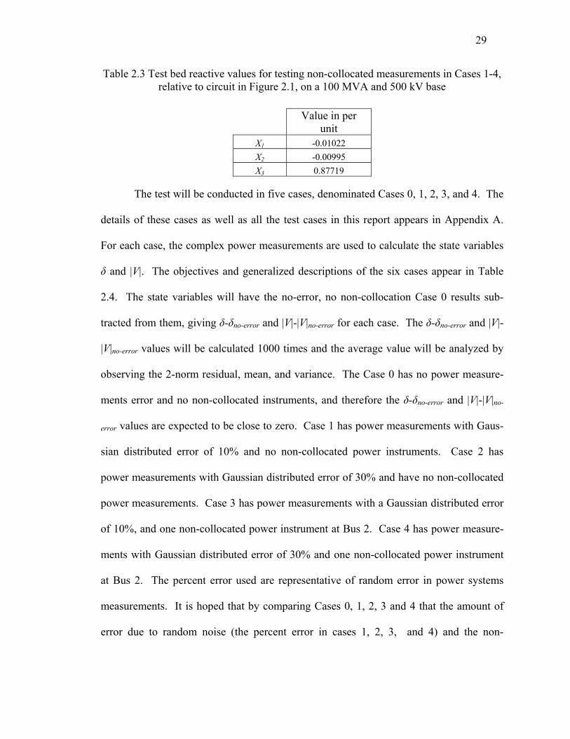
Table 2.3 Test bed reactive values for testing non-collocated measurements in Cases 1-4, relative to circuit in Figure 2.1, on a 100 MVA and 500 kV base

Value in per

unit X1 -0.01022 X2 -0.00995 X3 0.87719

The test will be conducted in five cases, denominated Cases 0, 1, 2, 3, and 4. The

details of these cases as well as all the test cases in this report appears in Appendix A.

For each case, the complex power measurements are used to calculate the state variables

δ and |V|. The objectives and generalized descriptions of the six cases appear in Table

2.4. The state variables will have the no-error, no non-collocation Case 0 results sub-

tracted from them, giving δ-δno-error and |V|-|V|no-error for each case. The δ-δno-error and |V|-

|V|no-error values will be calculated 1000 times and the average value will be analyzed by

observing the 2-norm residual, mean, and variance. The Case 0 has no power measure-

ments error and no non-collocated instruments, and therefore the δ-δno-error and |V|-|V|no-

error values are expected to be close to zero. Case 1 has power measurements with Gaus-

sian distributed error of 10% and no non-collocated power instruments. Case 2 has

power measurements with Gaussian distributed error of 30% and have no non-collocated

power measurements. Case 3 has power measurements with a Gaussian distributed error

of 10%, and one non-collocated power instrument at Bus 2. Case 4 has power measure-

ments with Gaussian distributed error of 30% and one non-collocated power instrument

at Bus 2. The percent error used are representative of random error in power systems

measurements. It is hoped that by comparing Cases 0, 1, 2, 3 and 4 that the amount of

error due to random noise (the percent error in cases 1, 2, 3, and 4) and the non-

30

collocated instrument (Cases 3 and 4 only) can be discerned. The results of test cases 0-4

are shown in Tables 2.5, 2.6, 2.7, and 2.8.

Table 2.4 State estimation Cases 0-4 testing criteria used with the 11 bus test bed

Case Objective Measurement

noise Non-collocated measurement

0 Base case None No 1 Low noise case 10% No 2 High noise case 30% No

3 Low noise, non-collocated measure-

ment 10% One, located at

bus 2

4 High noise, non-collocated measure-

ment 30% One, located at

bus 2

Table 2.5 Test bed average δ after 1000 runs compared to actual δ, for Cases 0-4 State δ-δno-error

Case Noise ||r||2 of δ (rad) Mean (rad) Variance (rad) 0 none 0.0945948 0.028521 1.62E-32 1 10% 0.0945958 0.028521 5.13E-09 2 30% 0.094598 0.028521 5.26E-08

3 10%, one non-

collocated meas-urement

0.095822 0.028521 2.39E-05

4 30%, one non-

collocated meas-urement

0.09586 0.028521 2.43E-05

Table 2.6 Test bed average |V| after 1000 runs compared to actual |V|, for Cases 0-4 State |V|-|V|no-error

Case Noise ||r||2 of |V| (p.u.

volts) Mean (p.u.

volts) Variance (p.u.

volts) 0 none 0.081075 -0.022879 8.18E-05 1 10% 0.081079 -0.022879 8.20E-05 2 30% 0.081119 -0.022879 8.11E-05

3 10%, one non-

collocated meas-urement

0.081558 -0.022879 8.88E-05

4 30%, one non-

collocated meas-urement

0.081511 -0.022879 8.92E-05

31

Table 2.7 Test bed average P measurement after 1000 runs compared to actual P, for Cases 0-4

P-Pno-error

Case Noise ||r||2 of P

(p.u.watts) Mean (p.u.

watts) Variance (p.u.

watts) 0 none 0.098162 -0.003115 5.57E-04 1 10% 0.107574 -0.006990 9.39E-04 2 30% 0.239030 -0.035610 0.002054

3 10%, one non-

collocated meas-urement

4.101085 -0.2225 0.929933

4 30%, one non-

collocated meas-urement

4.101085 -0.2225 0.934167

Table 2.8 Test bed average Q measurement after 1000 runs compared to actual Q, for Cases 0-4

Q-Qno-error

Case Noise ||r||2 of Q (p.u.

vars) Mean (p.u.

vars) Variance (p.u.

vars) 0 none 1.676460 0.008759 0.165243 1 10% 1.447761 0.086734 0.115952 2 30% 1.448581 0.084969 0.1149

3 10%, one non-

collocated meas-urement

2.16158 -0.006283 0.274566

4 30%, one non-

collocated meas-urement

2.155998 -0.003878 0.275201

2.3 Observations drawn from the example

The complex power in each test case is shown in Tables 2.7 and 2.8. In general,

the random measurement error in Cases 1 and 2 increases the 2–norm residual for P-Pno-

error and the mean of P-Pno-error for the active power deviates from zero (relative to the no-

error Case 0). For both the real and reactive power comparisons, the variance increases

due to measurement error. Subsequently, the measurement error alone increases overall

measurement error and variance. Cases 3 and 4 possess measurement error and a single

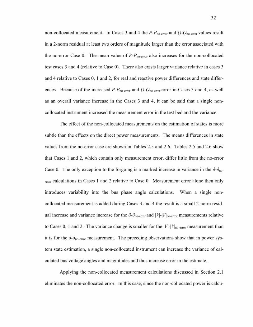
32

non-collocated measurement. In Cases 3 and 4 the P-Pno-error and Q-Qno-error values result

in a 2-norm residual at least two orders of magnitude larger than the error associated with

the no-error Case 0. The mean value of P-Pno-error also increases for the non-collocated

test cases 3 and 4 (relative to Case 0). There also exists larger variance relative in cases 3

and 4 relative to Cases 0, 1 and 2, for real and reactive power differences and state differ-

ences. Because of the increased P-Pno-error and Q-Qno-error error in Cases 3 and 4, as well

as an overall variance increase in the Cases 3 and 4, it can be said that a single non-

collocated instrument increased the measurement error in the test bed and the variance.

The effect of the non-collocated measurements on the estimation of states is more

subtle than the effects on the direct power measurements. The means differences in state

values from the no-error case are shown in Tables 2.5 and 2.6. Tables 2.5 and 2.6 show

that Cases 1 and 2, which contain only measurement error, differ little from the no-error

Case 0. The only exception to the forgoing is a marked increase in variance in the δ-δno-

error calculations in Cases 1 and 2 relative to Case 0. Measurement error alone then only

introduces variability into the bus phase angle calculations. When a single non-

collocated measurement is added during Cases 3 and 4 the result is a small 2-norm resid-

ual increase and variance increase for the δ-δno-error and |V|-|V|no-error measurements relative

to Cases 0, 1 and 2. The variance change is smaller for the |V|-|V|no-error measurement than

it is for the δ-δno-error measurement. The preceding observations show that in power sys-

tem state estimation, a single non-collocated instrument can increase the variance of cal-

culated bus voltage angles and magnitudes and thus increase error in the estimate.

Applying the non-collocated measurement calculations discussed in Section 2.1

eliminates the non-collocated error. In this case, since the non-collocated power is calcu-

33

lated from V2 and I1, then Case B from Section 2.1 would be the appropriate “fix.” The

“fix” (i.e., mathematical correction) is a software fix. After the power measurement ad-

justment, the Case 3 and 4 results would resemble the Cases 1 and 2 results. By compar-

ing Cases 1 and 2 to Cases 3 and 4, the benefits become apparent: there is a lower amount

of estimate variance and a lower 2-norm residual in Cases 1 and 2. Therefore, accounting

for non-collocated measurement increases state estimation confidence and creates more

accurate measurements system-wide.

34

CHAPTER 3 UNBALANCE FACTOR USE FOR SINGLE PHASE STATE ESTIMA-

TION IMPROVEMENT

3.1 Complex voltage and current unbalance factor

The voltage and current unbalance factors are a way of quantifying unbalance in a

three-phase power system. The three-phase current or voltage values can be decoupled

into the positive, negative, and zero-sequence components through the symmetrical com-

ponent transformation.

⎥⎥⎥

⎦

⎤

⎢⎢⎢

⎣

⎡=

⎥⎥⎥

⎦

⎤

⎢⎢⎢

⎣

⎡

−

+

0

][VVV

MVVV

c

b

a

, ⎥⎥⎥

⎦

⎤

⎢⎢⎢

⎣

⎡=

⎥⎥⎥

⎦

⎤

⎢⎢⎢

⎣

⎡

−

+

0

][III

MIII

c

b

a

,

23

211201 ja +−=°∠= ,

⎥⎥⎥

⎦

⎤

⎢⎢⎢

⎣

⎡=

11111

31

2

2

aaaaM and

⎥⎥⎥

⎦

⎤

⎢⎢⎢

⎣

⎡

=−

11111

31 2

2

1 aaaa

M .

The unbalance factor is a complex quantity used to quantify the amount of unbalance in a

power system, and is computed from the positive and negative sequence values,

+

−=IIU I and

+

−=VVUV .

Under balanced conditions, UI = UV = 0. Typically traditional power system instrumenta-

tion does not measure unbalance factor directly and software techniques are required.

However, many proposed methods exist for calculating the complex unbalance factor in a

system [16, 18], but this is often only for the voltage unbalance factor. It is also possible

35

to directly calculate the current or voltage complex unbalance factor if complete three-

phase phasor measurements are available, however this is rarely the case.

In many routine power engineering calculations, balanced conditions are assumed

[12, 13]. In a balanced three-phase power system, the negative and zero sequence values

are zero. This effectively simplifies a three-phase system into a single-phase system for

the purposes of various calculations. However, unbalanced conditions with negative and

zero sequence components are a reality in modern power systems [29]. There are many

causes of system unbalance, for instance single-phase loads and untransposed power lines

on crowded rights-of-way. Single-phase methods for state estimation can still prove ef-

fective even when unbalanced conditions are present in a small degree, but some power

systems may have enough unbalance to warrant a state estimation solution that takes into

account system unbalance. In communication with a major U. S. utility company, it is

found that only positive sequence voltages and currents are commonly reported and the

SCADA system, and therefore P+jQ is derived usually from (V+)(I+*). That is, negative

and zero sequence signals are ignored. Examples of the effect of unbalanced operation in

traditional state estimation calculations exist where the unbalance is taken from real data

and the effect on state estimation is noticeable [13]. This thesis seeks to use the unbal-

ance factor measurements in a power system to improve state estimation calculations,

utilizing their positive and negative sequence information.

Complex power measurements are often used in EMS state estimation programs

to find other values in a power system, like bus voltage magnitudes and bus angles. As it

has been stated earlier in this section, it is not uncommon for power utilities to operate

under a positive-sequence-only assumption for routine calculations. Some power utilities

36

may also only be monitoring a single phase at any point in the power system. If there are

only positive-sequence values in the system, then monitoring the voltage, current, and

complex power flow in a single phase is enough to calculate current, voltage, and com-

plex power in the two other phases through symmetrical component transformation.

When calculating the total, three-phase power flow at a point, the complete definition is

as follows,

.*00

**

***3

IVIVIVS

IVIVIVSS

Total

acnabnaanTotal

++=

++==

−−++

φ

This is true when the symmetrical component transformation matrix, M, is a hermitian

matrix, where M-1=MH, as follows,

⎥⎥⎥

⎦

⎤

⎢⎢⎢

⎣

⎡=

11111

31

2

2

aaaaM .

When there is a positive-sequence-only assumption, the negative and zero sequence com-

ponents are zero and the total complex power can be expressed more simply as,

.****3 acnabnaanTotal IVIVIVIVSS ++=== ++φ (3.1)

This three-phase power value in Equation (3.1) is correct in the balanced case. In the

proposed case of significant system unbalance, the value calculated in Equation (3.1) is

missing negative and zero sequence information.

If the power system has a significant negative sequence voltage and current, but

still a negligible zero-sequence component, then using the unbalance factor can lead to an

accurate, or at least improved (if a small amount of zero sequence current or voltage are

37

available), complex power value, S3 φ . It is said that zero-sequence components are small

regardless of the amount of unbalance present [16]. This is often the case since many

power transmission and distribution systems employ delta connected transformers which

block zero sequence components. A more accurate S3 φ value, which has negative se-

quence information, will then result in a more accurate set of results in state estimation.

This three-phase power calculation which features negative sequence information will be

as follows,

.*****3 acnabnaanTotal IVIVIVIVIVSS ++=+== −−++φ

Negative and positive sequence values can now be related to the unbalance factor, as fol-

lows,

⎥⎥⎥

⎦

⎤

⎢⎢⎢

⎣

⎡

⎥⎥⎥

⎦

⎤

⎢⎢⎢

⎣

⎡=

⎥⎥⎥

⎦

⎤

⎢⎢⎢

⎣

⎡

−

+

011111

31

2

2 VV

aaaa

VVV

cn

bn

an

)1(3

1)(3

1VVan UVUVVV +=+= +++

(3.2)

)(3

1)(3

1 22VVbn aUaVUaVVaV +=+= +++

(3.3)

)(3

1)(3

1 22VVcn UaaVUVaaVV +=+= +++

(3.4)

It will be assumed that only single-phase information is available from system measure-

ments (phase a). It will also be assumed that unbalance factor values are available.

Given these assumptions, there are three equations, Equations (3.2), (3.3), (3.4), with

38

three unknowns, V+, Vbn, and Vcn. Solving Equations (3.2), (3.3) and (3.4) for the un-

knowns yields,

V

an

UV

V+

=+ 13

)(1

2V

V

anbn Uaa

UV

V ++

=

)(1

2V

V

ancn aUa

UV

V ++

= .

Now all the voltages in the system are expressible with unbalance factor values and Va.

If all of the current values could be expressible with unbalance factor and the known sin-

gle-phase measurement Ia, then S3φ can be calculated exactly given the no zero-sequence

assumption. The symmetrical component transformation for current is the same as it is

for voltage and the unknown current values Ib, Ic and I+ can be derived the same way as

the unknown voltage-based values. This results in the following equations,

I

a

UI

I+

=+ 13

)(1

2I

I

ab Uaa

UI

I ++

=

)(1

2I

I

ac aUa

UI

I ++

= .

Using the above derived relationships, the complex power S3 φ is reevaluated in known

terms,

)(1

)(1

*2*

*2*

3 II

aV

V

anaan Uaa

UI

UaaU

VIVS +

++

++=φ

39

)(1

)(1

*2*

*2

II

aV

V

an aUaU

IaUa

UV

++

++

+

⎥⎥⎦

⎤

⎢⎢⎣

⎡+⎟

⎟⎠

⎞⎜⎜⎝

⎛

++

⎟⎟⎠

⎞⎜⎜⎝

⎛++

+⎟⎟⎠

⎞⎜⎜⎝

⎛

++

⎟⎟⎠

⎞⎜⎜⎝

⎛++

= 11111 *

*22

*

*22*

3I

I

V

V

I

I

V

Vaan U

aUaU

UaaU

UaaUaUa

IVS φ .

If a further assumption about the unbalance factor is made, that UV is negligible com-

pared to the generally much larger UI, then setting UV = 0 yields,

⎥⎦

⎤⎢⎣

⎡+

++

+++

= 11

11

1*

*2

*

**

3I

I

I

Iaan U

UaUaUIVS φ

[ ]**2**

*

3 121 III

I

aan UUaaUUIV

S +++++

=φ

*

*

3 13

I

aan

UIV

S+

=φ . (3.5)

It is reasonable to assume a small UV, since voltage bus magnitudes are generally

determined by low impedance (“stiff”) system. Given the assumptions that UV ≈ 0, UI is

known, and VanIa* are known, it is thought that the φ3S value calculated in Equation (3.5)

will yield more accurate state estimation results than S3 φ =V+I+* will alone, when unbal-

ance is present in the system. In the next section, this assumption will be tested in a small

test.

3.2 Test cases for observing the effect of the Equation (3.5) adjustment on state estima-tion

A small test bed has been prepared to study the effect Equation (3.5) can have on

state estimation. Equation (3.5) predicts the value of φ3S given the following assump-

tions,

40

• V0 = I0 = 0

• Van Ia* are known in phasor detail (i.e., magnitude and angle)

• UI is known in phasor detail at each measurement point

• UV is negligibly small.

A small three-phase test bed has been created with three buses. The test bed topog-

raphy is shown in Figure 3.1.

Figure 3.1 The three-bus test bed topology used in Cases 5-8 (lines and loads are three-phase)

The three-bus system shown in Figure 3.1 represents the system in picture detail.

The black diamonds show the location of complex power measurement instruments,

called M1, M2, M3 and M4. In this test bed, voltages and line reactance will be assigned

and the system parameters will be completely known. Each different test case will be

compared to this “perfect measurement” base case as a basis of judging quality.

Unbalance is introduced to the system for test purposes. The most common form

of unbalance in a system is unbalanced loads manifesting as unbalanced current [12]. For

41

the purposes of this test, line parameters have been kept equal on all three-phases phases

(representing fully transposed lines), but the voltage phase-neutral values are not bal-

anced. The unbalanced voltage magnitudes were kept within 5% of unity value and volt-

age angles differed by no more than 5º from their expected, balanced values (0°, -120°

and 120° for Van, Vbn, and Vcn, respectively). Small voltage unbalances will ensure that

the UV is small and therefore negligible, to fit the assumptions. As an example, if

⎟⎟⎟

⎠

⎞

⎜⎜⎜

⎝

⎛

°∠°−∠

°∠=

12500.112505.1000.1

,, cnbnanV ,

the voltage unbalance factor is 0.0463 .8.18 °∠

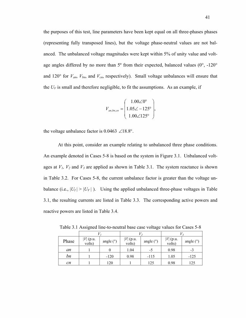
At this point, consider an example relating to unbalanced three phase conditions.

An example denoted in Cases 5-8 is based on the system in Figure 3.1. Unbalanced volt-

ages at V1, V2 and V3 are applied as shown in Table 3.1. The system reactance is shown

in Table 3.2. For Cases 5-8, the current unbalance factor is greater than the voltage un-

balance (i.e., |UI | > |UV | ). Using the applied unbalanced three-phase voltages in Table

3.1, the resulting currents are listed in Table 3.3. The corresponding active powers and

reactive powers are listed in Table 3.4.

Table 3.1 Assigned line-to-neutral base case voltage values for Cases 5-8 V1 V2 V3

Phase |V| (p.u. volts) angle (°) |V| (p.u.

volts) angle (°) |V| (p.u. volts) angle (°)

an 1 0 1.04 -5 0.98 -3 bn 1 -120 0.98 -115 1.05 -125 cn 1 120 1 125 0.98 125

42

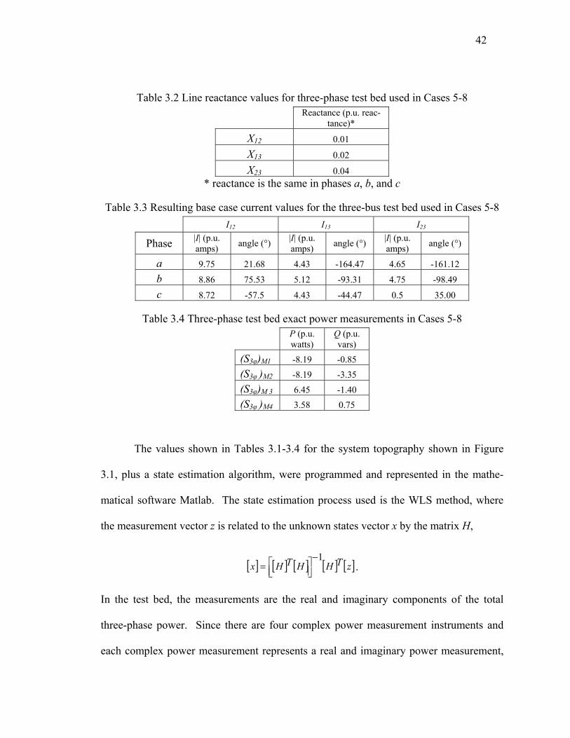
Table 3.2 Line reactance values for three-phase test bed used in Cases 5-8

Reactance (p.u. reac-

tance)*

X12 0.01

X13 0.02

X23 0.04 * reactance is the same in phases a, b, and c

Table 3.3 Resulting base case current values for the three-bus test bed used in Cases 5-8

I12 I13 I23

Phase |I| (p.u. amps) angle (°) |I| (p.u.

amps) angle (°) |I| (p.u. amps) angle (°)

a 9.75 21.68 4.43 -164.47 4.65 -161.12 b 8.86 75.53 5.12 -93.31 4.75 -98.49 c 8.72 -57.5 4.43 -44.47 0.5 35.00

Table 3.4 Three-phase test bed exact power measurements in Cases 5-8

P (p.u. watts)

Q (p.u. vars)

(S3φ)M1 -8.19 -0.85 (S3φ )M2 -8.19 -3.35 (S3φ)M 3 6.45 -1.40 (S3φ )M4 3.58 0.75

The values shown in Tables 3.1-3.4 for the system topography shown in Figure

3.1, plus a state estimation algorithm, were programmed and represented in the mathe-

matical software Matlab. The state estimation process used is the WLS method, where

the measurement vector z is related to the unknown states vector x by the matrix H,

[ ] [ ] [ ] [ ] [ ]zTHHTHx1−

⎥⎦⎤

⎢⎣⎡= .

In the test bed, the measurements are the real and imaginary components of the total

three-phase power. Since there are four complex power measurement instruments and

each complex power measurement represents a real and imaginary power measurement,

43

then the vector x has dimensions 8x1. The vector of states z will be made of the positive

sequence bus voltage magnitude and positive sequence bus voltage angle. Under the

positive-sequence only assumption, the total complex power can be related to purely

positive-sequence values. The vector z ignores Bus 1, since that bus has been chosen to

be the swing bus and will have a positive-sequence voltage magnitude of 3 p.u. at an-

gle 0° with zero negative and zero-sequence components (which is the result of the sym-

metrical component transformation for a balanced bus voltage where Va= °∠01 p.u.

Therefore, the vector z has dimensions 4x1, representing the voltage magnitudes and an-

gles at Buses 2 and 3.

Now the H matrix must be constructed to relate total power to the positive se-

quence voltage value. Since the assumption in the state estimator is only positive se-

quence values, the power flow calculation can be represented as a single-phase calcula-

tion in the positive-sequence system. The per unit value of the perfectly balanced power

system will give the following symmetrical components,

⎥⎥⎥

⎦

⎤

⎢⎢⎢

⎣

⎡

=⎥⎥⎥

⎦

⎤

⎢⎢⎢

⎣

⎡=

⎥⎥⎥

⎦

⎤

⎢⎢⎢

⎣

⎡

°∠°−∠

°∠=

⎥⎥⎥

⎦

⎤

⎢⎢⎢

⎣

⎡

−

+−

003

1201120101

0

1

VVV

MVVV

c

b

a

.

Because of this, the assumed positive sequence voltage magnitude is 3 p.u. under the

balanced system assumption. Real power flow in the positive-sequence system would

then appear as follows,

)sin( 2112

213 δδφ −= ++

XVV

P .

44

The positive-sequence voltage magnitude is assumed to be 3≈+V . The difference be-

tween positive sequence voltage angles is assumed to be small, therefore the value sin(δ1-

δ2) can be simplified to (δ1- δ2), resulting in the following relationship,

)(321

123 δδφ −≈

XP .

For the imaginary component of the complex power, the following relationship can be

used and simplified to construct the rest of the H matrix,

22

11

3

3

VV

VV

Δ+=

Δ+=

+

+

[ ]++++ Δ−Δ≈

Δ−= 21

212

13

3)cos(|||||| VVXX

VVVQ δφ .

This is reasonable simplification since the cosine of a small angle difference, such as

those between the voltage phases of adjacent buses in a somewhat balanced power sys-

tem, is very close to 1.0.

Each test case that will be carried out using the above outlined WLS method. The

difference between test cases will occur in the manner from which they gather their

power measurements. The first set of test cases, called Case 5, will calculate three-phase

power given only power measurements from a single-phase. The three-phase total com-

plex power is calculated from the single-phase measurement on the assumption that the

power system is completely balanced. The calculation method will appear as follows at

each measurement point to calculate the voltage at Buses 2 and 3,

abcCALCSECALC

a VVSS ⎯⎯ →⎯⎯→⎯⎯⎯ →⎯ +φ3

The resulting states from the state estimation will be compared to the base case for the

purposes of quantifying the error. The next test case, namely Case 6, also assumes sin-

45

gle-phase complex power awareness, but uses Equation (3.5) to calculate a different

three-phase power measurement. This test case will be called Case 6 and appear as fol-

lows,

abcCALCSECALC

Iaaa VVSUSIV ⎯⎯ →⎯⎯→⎯⎯⎯ →⎯ +φ3,,,

The results of this equation will also be compared to the base case states as well. Case 6

will be compared to Case 5 to see any improvement Equation (3.5) made in the state es-

timation. Table 3.5, shown later, summarizes these case conditions.

The next set of cases concern single-phase complex power awareness, but the sin-

gle-phase complex power is calculated from a three-phase power measurement. Al-

though the measurement loses no data through a balanced assumption, the state estima-

tion still assumes positive-sequence only conditions which may introduce error into the

results. The next test case will have a measurement vector of single-phase power, which

will called Case 7 and be carried by the following outline,

abcSE VS ⎯→⎯φ33

1

Since the solution to Case 7 will still have some error, Equation (3.5) will be used again

to see if there is any improvement. The new case is called Case 8 and will follow this

outline,

abcCALCSE

Ia VVUS ⎯⎯ →⎯⎯→⎯ +, .

These results can be compared to the base case states as well.

Each tests state estimation result will be compared to the perfect measurement

state and this result from each test case will be compared to find the most desirable out-

come from the test cases. The per-unit voltage magnitudes and the voltage angles for Bus

46

2 and 3 that result from each test cases state estimation will have the base case values

subtracted from them to for the residual, r. To compare the residuals from each test case,

the 2-norm residual value will be used. The norm calculation is used in mathematics to

quantify the size of a vector. If the estimated states were exactly correct, then the 2-norm

residual would equal zero. Larger 2-norm residuals will then indicate results that further

deviate from perfect values. The 2-norm residual calculation carried out to compare test

cases will look like as follows, where n is the number of states,

∑=

=−=n

kkPerfectTest rxxr

1

222 |||||||||| .

The state estimation calculation for each test case will be run once, without trying to

minimize the Jacobian value, as would occur in a more robust WLS state estimator.

Test Cases 5, 6, 7 and 8 will be carried out twice each, once with no error in the

measurements, again when a 10% error in the measurements has been introduced. The

10% error cases will be run 1000 times and the average 2-norm residual value from the

1000 runs will be used to compare to the other test results. The tests without error will

have the suffix “a,” whereas the tests with the 10% error introduced to the measurements

will have the suffix “b.” A key to the test names is shown in Table 3.5. Complete details

on all of the test cases within this thesis are available in Appendix A in Table A.1.

The Cases 5, 6, 7 and 8, with and without error, were calculated with MATLAB

software. The resulting state residuals are shown in Table 3.6.

47

Table 3.5 Key to identify test case names Test name ESS calculation method Measurement

error 5a Single phase power measurement none 5b Single phase power measurement 10% 6a Single phase power awareness with Equation (3.5) adjustment none 6b Single phase power awareness with Equation (3.5) adjustment 10% 7a Single phase power calculated from three-phase power measurement none 7b Single phase power calculated from three-phase power measurement 10%

8a Single phase power calculated from three-phase power measurement with Equa-tion (3.5) adjustment none

8b Single phase power calculated from three-phase power measurement with Equa-tion (3.5) adjustment 10%

Table 3.6 The 2-norm residuals of the difference between test states from case 5-8 and the base case states from Table 3.4 values

Test case names 5a 5b 6a 6b 7a 7b 8a 8b

|V2| (p.u. volts) 0.04486 0.04486 0.04366 0.04366 0.04322 0.04322 0.04373 0.04372 δ2 (rad) 0.17565 0.17569 0.14323 0.14324 0.14254 0.14255 0.14321 0.14322 |V3| (p.u. volts) 0.05945 0.05946 0.05844 0.05844 0.05761 0.05761 0.05770 0.05770 δ3 (rad) 0.13061 0.13061 0.13917 0.13918 0.13066 0.13069 0.14329 0.14328

Table 3.7 The 2-norm of the residuals between raw state estimates from Cases 5-8 and base case estimates from Table 3.4 values

|| exactxx−^

||2 || exactxx−^

||2

5a angle (rad) 0.05744 7a angles (rad) 0.11917

6a angle (rad) 0.03012 8a angles (rad) 0.03624

5a |V| (p.u. volts) 0.02137 7a |V| (p.u.

volts) 0.04279

6a |V| (p.u. volts) 0.01709 8a |V| (p.u.

volts) 0.00307

3.3 Observations drawn from test cases

By comparing the state estimated phasor voltage values for Bus 2 and 3 to the base

case state values, the impact of Equation (3.5) in state estimation for this test bed be-

comes apparent. One observation is that the introduced measurement error had little ef-

48

fect on the test results. The resulting residuals are the same to four decimal places. Be-

cause of this, what is said about the results from Case 5a is true for Case 5b. The results

in Table 3.6 show that the states calculated in Case 6 were an improvement over the cases

calculated in Case 5. To quantify the difference, the percent difference calculation is

used,

%100*

2

%21

21

⎟⎠⎞

⎜⎝⎛ +

−=

tmeasurementmeasurementmeasurementmeasuremen

difference .

The voltage angle residuals from Case 6 had a 2.71% and 1.71% percent difference from

the Case 5 voltage angles. The percent difference between the voltage magnitude states

between Case 5 and 6 is much more profound, equaling 20.33% and 6.35% (although the

Case 5 result for the voltage angle at Bus 3 was closer).

The difference between Cases 6, 7 and 8 are the same to two decimal places and all

are an overall improvement compared to the Case 5 results. Case 8, which uses the Case

7 method but with the Equation (3.5) adjustment factor, is very close to the Case 7 re-

sults, but offers no improvement for any of the states calculated.

However, the above residuals were calculated from the processed states. That is,

the raw states are the positive sequence voltages at Bus 2 and 3 (or the phase a voltage at

Bus 2 and 3 in the case of Case 7) are then used to calculate the phase-to-neutral voltages

at Bus 2 and 3, assuming balance. When the raw residuals are compared to the base case

answers and the 2-norm taken, the results seem more promising, as seen in Table 3.7. In

each case the state estimator using the Equation (3.5) adjusted power value produced su-

49

perior results. It is during those results transformation into phase-to-neutral voltages that

the results become less impressive.

Since the test bed is small relative to large power systems and the values arbitrary,

it is difficult to predict the impact of the Equation (3.5) adjustment factor on a large-scale

power system state estimation algorithm. If a larger test bed were used along with actual

measurement data, then perhaps a clearer picture of the adjustment factors effect can be

gained. A more robust and complete state estimation algorithm may also show an im-

proved picture of the adjustment factors effect. It is also unknown how feasible current

unbalance factor measurement throughout a power system is, which will be explored in

the next section. However, the adjustment factor may have a worthwhile effect on state

estimation results for an unbalanced system that makes SE calculations assuming bal-

anced conditions, with only single-phase awareness.

3.4 Notes on calculating complex unbalance factor without phasor measurements

It should be noted that the complex current unbalance factor, which is used exten-

sively in Chapter 3, is not a commonly metered value. CUF may be easily calculated

when three-phase phasor detailed measurements are available, which is increasingly fea-

sible due to the implementation of GPS technologies, however much more common in

power utilities are still the traditionally metered values: power flow, injected power, volt-

age magnitudes and current magnitudes [33]. Fortunately even in a power system where

only traditional metered values are reported there are ways to calculate the complex un-

balance factor, both VUF and CUF, without new or special equipment. Many of these

methods rely on phasor mathematics and only use the per-phase voltage or current mag-

50

nitudes. Even when the unbalance factor cannot be calculated exactly, it may be worth-

while to calculate an estimate, which will be discussed later in this section.

Represented in the literature there are phasor-detailed voltage unbalance factor cal-

culation methods utilizing the three-phase voltage magnitudes. Often line-to-line voltage

magnitude data are available [18], for which there are many methods for calculating the

complex VUF. The line to line voltage phasors can be drawn in a triangle configuration.

This triangle, with known side-lengths (phasor magnitudes) but unknown angles, contains

the angle information of the phasors discerned from trigonometric properties (e.g., the

law of cosines). This “voltage triangle” method, where the complex VUF is directly cal-

culated from the line-to-line voltage magnitudes, is presented in detail in [18]. Wagner

[32] also shows that the voltage phase angles can be calculated from the three line-to-

neutral voltage magnitudes, but only in the absence of a zero-sequence component. Once

the voltage phase angles are known along with the magnitudes, the symmetrical compo-

nents and the unbalance factor can be directly calculated.

Of primary concern for this thesis, however, is the complex current unbalance fac-

tor, which is used extensively here. Unlike line-to-line voltage phasors, the current

phasors do not always form a closed triangle at any point. However, in ungrounded wye

or delta connected systems, such as those in some loads and transformers, the current

phasors will sum to zero because without a neutral these currents are subject to

Kirchhoff’s current law. Presented later in this section is a method for direct calculation

of the CUF given the three per-phase current magnitudes, given the presence of an un-

grounded delta or wye connection at the point of measurement. For more general cases,

51

the effects of estimating the phase angles of the current in unbalance factor calculation

will now be explored.

Electrical current instrumentation traditionally reports a current magnitude and may

or may not report all three phases. Assumptions about phase angles may help estimate

CUF. This estimated CUF, when used to calculate the three-phase power at a point, as in

Equation 3.5, may improve state estimation in an unbalanced power system. To test the

value of estimated current unbalance factor, two sets of estimation criteria were devel-

oped.

The first CUF estimation method developed was presumes two current magni-

tudes are available, called |Ia| and |Ib|. This estimation method would be appropriate in a

system where single-phase current magnitude sensors are augmented with a single clamp-

on CT, or other instrumentation method. The phase a current was assigned an angle of

zero and the phase b current was assigned an angle of 120°, which are the expected val-

ues in a balanced system. The assumption being the unbalance is primarily in the current

magnitudes, not the angles. The final current phase, Ic, is calculated as follows, assuming

an ungrounded wye or delta connection,

abc III −−= .

These current values were used to calculate the current symmetrical components and then

the UI at each measurement point in the test bed developed in Section 3.2. When com-

pared to the actual complex CUF values from the test bed, the UI magnitude at any meas-

urement point differed from as little as 4.7% and as much as 99.8% from the actual UI

magnitude. The angle for the estimated UI differed as little 2.4% and as much as 37.9%

52

from the actual angle. There is clearly some error from the estimation, but the state esti-

mation results were developed to see if the error is sufficiently negligible. Table 3.8

shows the result from the estimated CUF in the test bed data, where a residual is calcu-

lated from the test state estimation results and the actual state values. Much like the re-

sult tables in Section 3.3, Cases 6 and 8 use the S3φ calculation from Equation 3.5 to im-

prove state estimation (only with the estimated UI used in the S3φ calculation this time).

Case 5 has the states calculated from single-phase data under a balanced operation as-

sumption and Case 8 is still state estimation calculated from three-phase data under a bal-

anced system assumption. Case 6 has a smaller residual compared to Case 5 and Case 8

has a smaller residual compared to Case 7, signifying an improvement when Equation 3.5

is employed, even with the estimated UI value. Comparing the 2-norm residuals from

Table 3.8 to that of the “exact” UI case in Table 3.7 reveals that while both methods offer

an improvement, that the “exact” UI case has superior results, which is to be expected.

However, the differences are small and despite the sometimes large difference between

the calculated UI and the true UI, the results are still superior compared to the states esti-

mated under the balanced operation assumption alone.

Table 3.8 Normalized state estimate residuals from the three-phase test bed utilizing the two-magnitude, estimated UI method, using Cases 5-8 system data

|| exactxx−^

||2 || exactxx−^

||2

5a angles (rad) 0.05744 7a angles (rad) 0.11917

6a angles (rad) 0.03098 8a angles (rad) 0.04860

5a |V| (p.u. volts) 0.02137 7a |V| (p.u.

volts) 0.04279

6a |V| (p.u. volts) 0.01263 8a |V| (p.u.

volts) 0.01184

53

The assumption-based CUF estimation will now be studied again, but this time

with all three current magnitudes presumed known, rather than only two as was used be-

fore. This could represent a situation where three-phase current magnitudes are metered

or single-phase current instruments have been augmented. In a similar fashion to the

previous test, the phase a current is assigned an angle of zero, the phase b current is as-

signed an angle of 120°, and the phase c current has known magnitude and satisfies the

following,

abc III −−= .

This method contains additional information over the last assumption-based method (the

phase c magnitude is known). These estimated CUF values were again calculated from

the Section 3.2 test bed and compared to the actual UI values. The UI angles differed by

as little as 0.3% to as much as 80.2% from the actual. The UI magnitudes differed by as

little as 23.72% to as much as a stunning 649.17%. Again the assumption-based UI are

used in the Equation 3.5 calculation, resulting in the 2-norm residuals of the states com-

pared to the base case values shown in Table 3.9.

Table 3.9 Normalized state estimate residuals from the three-phase test bed utilizing the three-magnitude, estimated UI method, using Cases 5-8 system data

|| realxx−^

||2 || realxx−^

||2

5a angles (rad) 0.05744 7a angles (rad) 0.11917

6a angles (rad) 0.04728 8a angles (rad) 0.04860

5a |V| (p.u. volts) 0.02137 7a |V| (p.u.

volts) 0.04279

6a |V| (p.u. volts) 0.01416 8a |V| (p.u.

volts) 0.00845

54

Despite the added information, the resulting states offer results better and worse

than those of the |Ia| and |Ib| method in Table 3.8. This may be due to the singularly large

estimated UI magnitude error in the test data. What is clear is that the assumption based

UI calculation method paired with the Equation 3.5 method may offer an advantage for

calculating states in an unbalanced three-phase system.

While the Table 3.8 and 3.9 results show the estimated UI method can give superior

results to the balanced operation assumption alone, the Equation 3.5 method for improv-

ing state estimation parameters is designed for the exact UI value. Under special circum-

stances, the CUF can be calculated from the three-phase current magnitudes in a similar

manner to the VUF calculation methods presented earlier in this section. When the three-

phase currents sum to zero (or are assumed to do so), the resulting phasors can be drawn

in a closed triangle (see Figure 3.2). This is the case at any ungrounded wye or delta con-

nection.

Figure 3.2 Three-phase current phasors that sum to zero

Through the law of cosines the angle between phase a and b can be described as

follows,

aI

bI cI

αΘ

55

||||2||||||

cos222

ba

bac

IIIII

−−−

=θ .

The angle complimenting θ in Figure 3.1 is called α and since cos α=-cos θ,

||||2||||||cos222

ba

bac

IIIII −−

=α . (3.6)

The numerator and denominator in Equation 3.6 can be said to describe a triangle, shown

in Figure 3.3.

Figure 3.3 Right triangle from angle α and law of cosines relationship

Using this information and knowledge of the three-phase current magnitudes, the

complex current unbalance factor can be derived. The first step is setting the phase a cur-

rent as the reference current with angle zero,

°∠= 0|| aa II .

The angle α derived earlier describes the relative angle between phase a and phase b,

whereas the phase b current can be described in rectangular notation as,

( )αα sincos|| jII bb += . (3.7)

ba II2

222abc III −−

( )22224 abcba IIIII −−− α

56

The cosα portion of Equation 3.7 is described in Equation 3.6. The sinα portion of Equa-

tion 3.7 may be derived from the right triangle presented in Figure 3.3, which is as fol-

lows,

||||2)|||||(|||||4

sin222222

ba

bacba

IIIIIII −−−

=α .

The final calculation for Ib is as follows, where the sign for the square root portion is arbi-

trarily chosen to be negative to reflect the tendency for positive sequence over negative

sequence in a power system,

.||||2

)|||||(|||||4||||2

|||||| 222222222

ba

bacba

ba

bacb II

IIIIIj

IIIII

I−−−

−−−

=

Since the current phasors form add up to zero, the c phase current is simply calculated as,

abc III −−= .

Using the three current phases described in phasor detail, the symmetrical compo-

nents are calculated, which is used to find the complex current unbalance factor. Multi-

plying by the symmetrical component transformation matrix, with the symmetrical trans-

formation matrix coefficient ignored since it will divide out in the unbalance factor equa-

tion, the following symmetrical components result,

||||2)|||||(|||||4 222222

ba

bacba

IIIIIII

M−−−

±=

23

211201 j+−=°∠=α

cba IIII 2αα ++=+

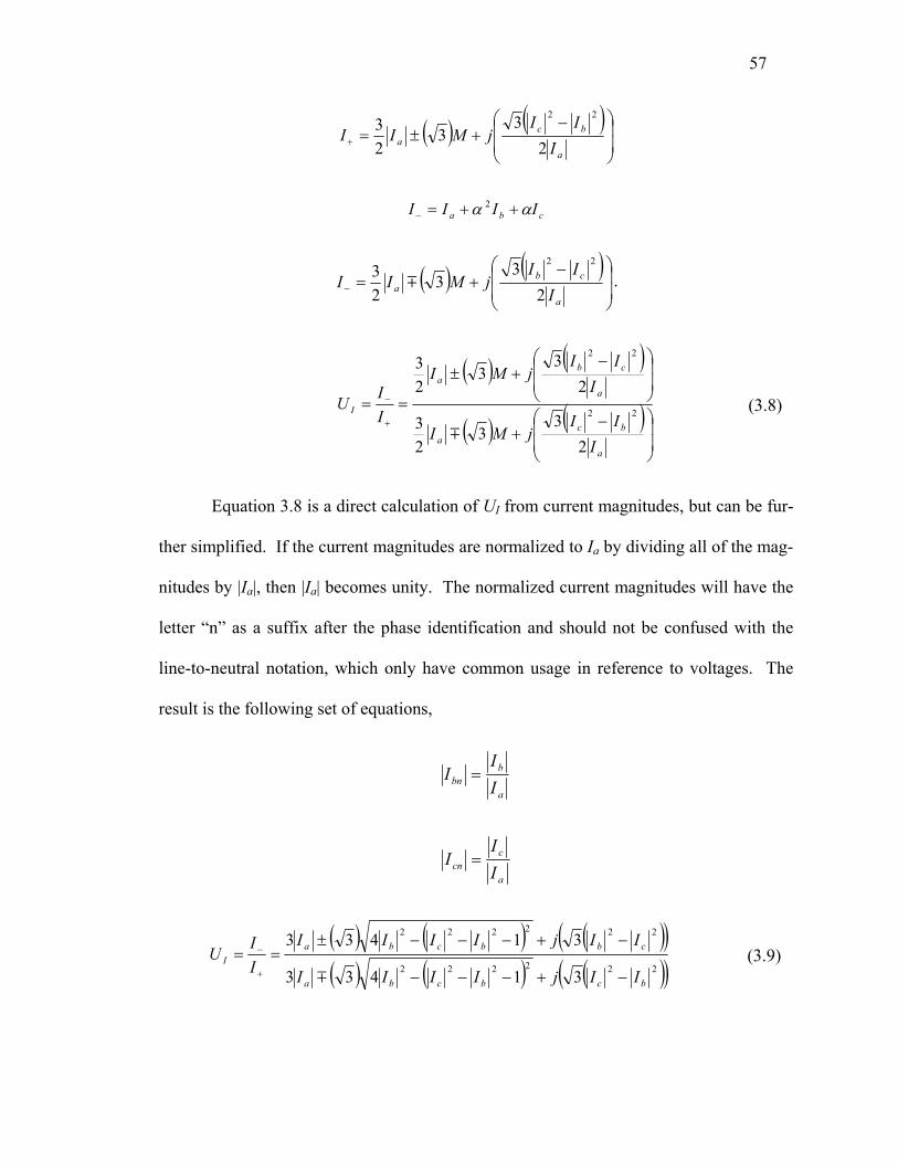
57

( ) ( )⎟⎟

⎠

⎞

⎜⎜

⎝

⎛ −+±=+

a

bca I

IIjMII

23

323

22

cba IIII αα ++=−2

( ) ( )⎟⎟

⎠

⎞

⎜⎜

⎝

⎛ −+=−

a

cba I

IIjMII

23

323

22

m .

( ) ( )

( ) ( )⎟⎟

⎠

⎞

⎜⎜

⎝

⎛ −+

⎟⎟

⎠

⎞

⎜⎜

⎝

⎛ −+±

==+

−

a

bca

a

cba

I

III

jMI

III

jMI

II

U

23

323

23

323

22

22

m

(3.8)

Equation 3.8 is a direct calculation of UI from current magnitudes, but can be fur-

ther simplified. If the current magnitudes are normalized to Ia by dividing all of the mag-

nitudes by |Ia|, then |Ia| becomes unity. The normalized current magnitudes will have the

letter “n” as a suffix after the phase identification and should not be confused with the

line-to-neutral notation, which only have common usage in reference to voltages. The

result is the following set of equations,

a

bbn I

II =

a

ccn I

II =

( ) ( ) ( )( )( ) ( ) ( )( )222222

222222

31433

31433

bcbcba

cbbcbaI

IIjIIII

IIjIIIIII

U−+−−−

−+−−−±==

+

−

m

(3.9)

58

Due to the square root calculation for the M value, there is an ambiguity of sign.

Through experimentation, it has been shown that for predominately positive sequence

systems, where the phase b current has a negative angle in reference to phase a, the M in

the numerator is negative and the M in the denominator is negative. When phase b has a

positive angle in reference to phase a, then the M in the numerator is positive and the M

in the denominator is negative. Since the positive sequence current is often larger than

the negative sequence current, even in unbalance, the positive sequence answer for the

unbalance factor calculation may be assumed. The following equation illustrates this

value,

( ) ( ) ( )( )( ) ( ) ( )( )222222

222222

31433

31433

bcbcba

cbbcbaI

IIjIIII

IIjIIIIIIU

−+−−−+

−+−−−−==

+

− . (3.10)

Equation 3.10 allows exact calculation of the complex CUF, if the current Ia is

taken as the reference value (angle is zero). In the absence of metering of the UI value or

three-phase current phasor measurements, this can make the Equation 3.5 three-phase

power calculation possible and improve state estimation in an unbalanced system.

3.5 Summary of results

The formula derived earlier in this section, called Equation 3.5, makes it possible

to calculate three-phase complex power from a single phase complex power measurement

and the complex current unbalance factor, if voltage unbalance and negative sequence

information are both negligible. This has many advantages in state estimation, including

making three-phase measurements possible from single-phase measurements, when the

59

complex CUF is known. Many situations where Equation 3.5 might improve measure-

ments were modeled and studied. The question of calculating the complex current unbal-

ance factor where direct measurements are not available was also tested, as well as the

viability of estimating the complex CUF.

Test Cases 5-8 were conducted to show how use of Equation 3.5 on system meas-

urements may improve state estimation results for a hypothetical 3 bus power system. In

general, Cases 5-8 operate on an assumption of balanced conditions and perform WLS

under that assumption. The details of Cases 5-8 can be found in Section 3.2 and the de-

tails of the Cases 5-8 are outlined in Table 3.5. The results of these Cases are shown in

tables 3.6 and 3.7, where the 2-norm of the first iteration state estimations residuals is

compared. In general, Equation 3.5 yielded improved first iteration state estimation re-

sults compared to similar cases that did not use Equation 3.5.

In Section 3.4, the viability of estimating the complex current unbalance factor was

examined and calculations similar to Cases 5-8 were performed, utilizing the three-bus

test bed. The complex current unbalance factor estimation criteria used created CUFs

that were sometimes close to the exact value and sometimes very much different. De-

spite the mixed results in estimating complex CUF, Cases 5-8 were run again and again

showed improved first iteration state estimation results under the testing criteria, however

the improvement less compared to when the exact complex current unbalance factor was

known.

Next a method for directly calculating the current unbalance factor from three-phase

current magnitude measurements was presented. The method requires three-phase cur-

rent magnitude measurements and must be at an ungrounded delta or wye connection.

60

CHAPTER 4 LINEAR PREDICTION METHODS FOR NON-SIMULTANEOUS

MEASUREMENT CORRECTION TO IMPROVE STATE ESTIMATION

4.1 Non-simultaneous measurements

State estimation relies on measurement inputs which may have no time stamp.

Because of this, measurements with time delay could be erroneously accepted as simulta-

neous (no delay) by state estimation algorithms. The measurement may be flagged as

being in error; however, the error may be identified as measurement error. Delayed

measurements in a power system are a real concern and can be caused by a variety of

sources. Communication systems can be a source of measurement delay, for instance if

there is not have enough bandwidth to accept all measurements in a timely fashion. In-

struments may also operate on delayed clocks, although with GPS technology to syn-

chronize time signals this to may be increasingly less common in modern systems. More

prevalent are time delays caused by the cooperation between separate but interconnected

power entities, where information is exchanged, possibly through a central power pool.

Power entities may be inclined to incorporate interconnected power system measurement

and state information, but differences in communication, timing, and other operational

issues can manifest themselves in a delay of a few seconds for real time measurements

and a delay of as much as 60 minutes for state estimation results [23], [29]. Furthermore,

these delays may be of unpredictable occurrence and length. Some instruments, most

notably phasor measurement units (PMUs), offer time stamping on their readings. A

PMU is a GPS based instrument which utilizes four or more signals from GPS satellites

to obtain an absolute time. Using absolute time as a time stamp, the PMU can fit a “best”

61

sine wave to a voltage or current measurement and thereby make a phasor measurement.

Until PMU use becomes more widespread, time stamping may be an unrealistic solution

to measurement delay problems. Even when time stamps are available, interpolation

software may be needed to correlate (match) measurements.

Many stochastic prediction techniques exist in the literature to improve delayed

measurements, including auto regressive-moving average techniques, Winter’s multipli-

cative seasonal model, and Kalman filtering techniques [22-23], [29], [35]. These algo-

rithms may rely on measurements with known latency delay lengths; measurements with

a known delay probability (i.e., a known or assumed statistical model for latency); meas-

urements with a known or assumed dynamic model such as forcing functions. The effort

here is to explore the use of a simpler linear process that operates with less required in-

formation to improve delayed measurements and the resulting state estimation.

4.2 Linear measurement prediction

A linear, autoregressive process is considered for signal prediction, which will

take the general form,

1

^

1 mxnxmxnzAz = . (4.1)

A measurement vector is defined as n consecutive sampling time periods in length (the

vector z in (4.1)). The vector z is multiplied by a relation matrix A to form a measure-

ment prediction z , at time t. This is accomplished using the algorithm presented in Fig-

ure 4.1.

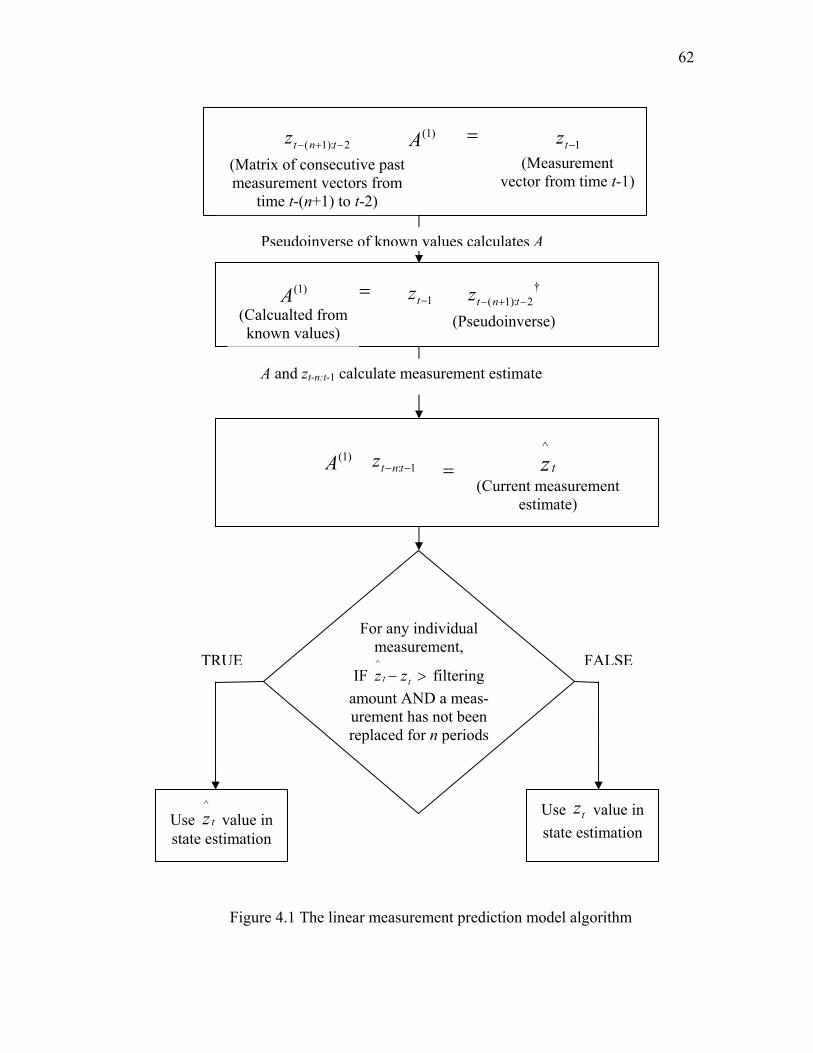
62

Figure 4.1 The linear measurement prediction model algorithm

2:)1( −+− tntz (Matrix of consecutive past measurement vectors from

time t-(n+1) to t-2)

)1(A 1−tz (Measurement

vector from time t-1)

=

=)1(A (Calcualted from known values)

1−tz †

2:)1( −+− tntz (Pseudoinverse)

)1(A 1: −− tntz = tz

^

(Current measurement

estimate)

Use tz^

value in state estimation

TRUE

Use tz value in state estimation

FALSE

For any individual measurement,

IF >− tt zz^

filtering amount AND a meas-urement has not been replaced for n periods

Pseudoinverse of known values calculates A

A and zt-n:t-1 calculate measurement estimate

63

As shown in Figure 4.1, a value of A is calculated from a set of recent, consecutive

measurements in memory, where A is calculated by multiplying the measurement vector

from time t-1 to the pseudo-inverse of the matrix of past measurement vectors from time

t-n+1 to t-2. This A is used as an estimate for the A which relates the measurements from

time t-n to t-1 to the measurement at time t. This method makes very accurate predictions

of a signal (assuming noiseless measurements) if:

• The sampling time period used to take measurements is frequent relative to the

rate of change of the signal being measured.

• The past number of measurements in memory (n+1) is sufficiently large (in

practice, at least 3 or more for good predictions, see the test cases for more de-

tail).

These are reasonable assumptions for a power system under normal conditions in

the absence of high speed dynamics (so-called “stable” conditions). Power system meter-

ing may sample several times a second, therefore during normal operation the rate of

change of typical measurements, like real and reactive power, will likely be small com-

pared to the possible measurement sampling rate. Note that the term “stable” does not

refer to system stability in this case; rather, the tern is used to describe system dynamics

that are not highly varying.

Intuitively, large amounts of measurements kept in memory may yield better es-

timation results compared to smaller numbers of measurements. Larger blocks of past

measurements will add more information to the linear prediction model and, when de-

layed measurements are present, allow for more non-delayed measurements to influence

the prediction model. This assumption will be tested later in this section.

64

However, a problem with delayed measurements in a power system is that they

are not perfect measurements. The appearance of a randomly delayed measurement in a

continuous set of data is presented in Figure 4.2. The delayed measurements used in the

linear prediction model as presented in Figure 4.1 may add error to the prediction result.

The challenge then is to find ways to optimize this prediction model, such that the predic-

tions are appreciably better than the delayed measurement signal alone. Making the lin-

ear prediction algorithm give superior results has the following challenges:

• Have enough past measurements in memory to allow for better predic-

tions.

• Not having as many past measurements in memory as to cause storage is-

sues or burdensome amounts of additional calculation.

• Having a large number of measurements compared to the rate of change in

the measurement signal.

• Creating a set of past measurements accurate enough to make usable pre-

dictions.

The logical next step would be to use the corrected measurement signal produced

by the linear algorithm and use this corrected value in the next step of the prediction

method, however this can be problematic. Use of corrected measurements in the linear

prediction method can result in large prediction errors relative to the uncorrected delayed

signal, which in turn introduces even greater error into the prediction algorithm. Exam-

ples of delayed measurement signals and the “spikes” this information can cause in the

prediction output are presented in Figure 4.3. When these errors, large relative to the de-

65

layed measurements, are used in the signal prediction estimator, the error compounds and

the prediction error can grow several orders of magnitude. Because of this, the delayed

measurement signal is selected to be used in the linear prediction algorithm since it is the

least problematic of the choice of signals. The challenge then becomes one of finding a

way to improve the linear algorithm given the delayed input.

Figure 4.2 An example of a randomly delayed measurement signal with sampling period 0.5 s and P measured in per unit, from Case 9a

The solution found to the “prediction spikes” was to avoid making a measurement

correction as long as a suspected delayed measurement is in memory. In short, if n per-

vious time periods are in memory, then only one delayed measurement replacement can

be performed during n time periods.

This prediction improvement strategy adds the following concerns to the linear

prediction method:

66

• The previous measurements in memory n cannot be too large; otherwise the

correction method is hardly used.

• The replacement algorithm will not correct every delayed measurement, but

should produce an improved set of measurements for state estimation.

• Since only one measurement replacement per n time periods is performed,

the probability of delayed measurements should be small over this time pe-

riod to avoid not correcting a large amount of delayed measurements.

Figure 4.3 An example of the randomly delayed measurements effect on the linear pre-

diction algorithm, from Test Case 9a

With this new improvement to the algorithm shown in Figure 4.1, the testing phase

was conducted.

4.3 Test case to find optimal linear prediction method

67

The general linear signal prediction method was used on test data to find what the

optimal linear prediction algorithm. A test bed power system was created in Matlab, with

sample code provided in Appendix B. The test power system is an invented five bus

power system, with seven instruments that measured real power flow. No |V| prediction

was attempted. The power flow equation used was as follows,

( )212121 1)sin( δδδδ −≈−=

XXVV

P .

The familiar weighted least squares state estimation equations was compiled where the

state vector x was composed of the bus voltage angles, the measurement vector z was

composed of real power measurements, and the relationship matrix H was composed of

1/X values relative to the above power flow equation, shown here,

Hxz = .

The five bus, seven instrument power system is shown in Figure 4.4. The topog-

raphy was invented, as were the line reactances. Power measurements are invented,

where each instrument was assigned a separate non-repeating sinusoid value for its power

reading, with similar bandwidth. Power and reactance values are in per unit. Bus angles

are in radians.

Several different test cases were conducted to study the linear measurement pre-

dictions benefit in different systems. All of the test cases had this in common: each

measurement had a 5% chance of being delayed by one time period. The proposed algo-

rithm shown in Figure 4.1 allows for several different variables, with each combination

representing a test case: the A matrix was either calculated once for the testing period

(Cases 9, 10, 12 and 13) or continuously updated (Cases 11 and 14), the A matrix was

68

calculated from randomly delayed measurements (Cases 9 and 11) or from “perfect”

measurements (Cases 10 and 12), from noiseless signals (Cases with suffix “a”) and sig-

nals with a random measurement error of up to 10% the real value (Cases with suffix

“b”), and finally cases with power signals of relatively high bandwidth (1.5 radians/time-

period, Cases 12-14) to cases with relatively low bandwidth (0.15 radians/time-period,

Cases 9-11). The differences between the different cases are outlined in Table 4.1 and in

Appendix A.

The different test cases were performed to study the performance of the linear test

method. One difficulty which immediately became apparent was the choice of signal for

calculating the A matrix: the corrected signal, or the uncorrected signal with random de-

lays. It was found that using the delayed measurements in the predication algorithm

would cause poor predictions. Measurements without delay kept in memory would pro-

duce good predictions, but as soon as a delayed measurement was introduced into mem-

ory it would cause an error in the prediction, often greater than the error of a delayed

measurement. This is illustrated in Figures 4.2 and Figure 4.3.

Figure 4.4 The five bus test bed for Cases 9-14

69

Table 4.1 Identities of test Case 9-14 Case A matrix Measurement error Signal bandwidth 9a calculated once (delayed) None 0.15 radians/time period 9b “ 10% " 10a calculated once (no delay) None " 10b “ 10% " 11a updated continuously None " 11b “ 10% " 12a calculated once (delayed) None 1.5 radians/time period 12b “ 10% " 13a calculated once (no delay) None " 13b “ 10% " 14a updated continuously None " 14b “ 10% "

Several sets of criteria were used to rank the different test case results. One was

the minimum length n of the past measurement matrix needed to produce measurement

predictions that are better than the delayed measurements most of the time. Another cal-

culation performed was the 2-norm residual of the delayed measurements subtracted from

the real measurements, and the 2-norm of the corrected delayed measurements subtracted

from the real measurements. The linear prediction method residuals were calculated at an

n value that produced more prediction values closer to the exact signal than delayed sig-

nal values closer to the actual signal. The results are shown in Table 4.2.

Analyzing the results in Table 4.2 shows the strengths and weaknesses of the lin-

ear prediction method.

• A 2-norm residual closer to zero is deemed the more desirable result, since the

test results were closer to the actual values. For instance, the test runs with the

“b” suffix, where random 10% noise is added, are always less desirable than the

noiseless solutions.

70

• Cases with a higher change in signal per sampling time period (Cases 12-14)

gives results less desirable than those in the low change cases (Case 9-11).

• Cases where the A relationship matrix is not continually calculated (Cases 9-10,

12-13) also give improved results compared to continually updated cases (Case

11, 14).

• When A is calculated once, it is advantageous to use measurements without delay,

such as in Cases 10 and 13. This may be done during a period of low latency to

“tune” the algorithm.

Table 4.2 Results for test Cases 9-14 2-norm of measurement

residual 2-norm of state residual

Case Min size

n

Size n

used in

test Delayed signal

Corrected signal

Delayed signal

Corrected signal

9a 5> 5 0.1829 0.1539 8.603e-4 6.178e-4 9b 10> 10 3.6675 3.4935 .06794 .06757 10a 10> 10 0.1453 0.0852 7.9785e-4 6.5072e-4 10b 10 10 3.7674 3.8874 .0667 .0664 11a 5-17 10 0.1120 0.1265 8.6173e-4 5.6278e-4 11b 15> 15 3.5170 13.4748 0.0650 0.2021 12a 3-13 3 0.8536 1.2795 0.0137 0.0130 12b 60> 60 2.9117 50.4776 0.0543 0.4923 13a 3-15 3 0.8572 0.5729 0.0123 0.0063 13b 50> 50 2.9394 45.0016 0.0562 0.3966 14a 6-8 7 0.9306 1.3935 0.0146 0.0156 14b 30> 30 3.2545 41.6380 0.0524 0.3548

Many things about the linear prediction method can be inferred from these gener-

alized results. For instance, A should not be continually updated, since it is computation-

ally more expensive and offers no discernable advantage. Also, low measurement noise

is preferable. The argument is made for the value of pre-estimation noise filtering.

71

When only 10% noise is added to the test bed, the linear algorithm cannot offer improved

results, probably due to larger “prediction spikes” like those shown in Figure 4.3.

Power systems with a low probability of delayed measurements per time period

during times of low system change may derive a benefit from this linear measurement

correction algorithm. However, noisy, chaotic systems may not. Power systems where

this prediction algorithm is not appropriate may instead benefit from the stochastic cor-

rection algorithms presented in the literature that require a more in-depth study of the

cause and model of delay.

72

CHAPTER 5 CONCLUSIONS AND RECOMMENDATIONS

5.1 Conclusions

The main conclusions of this work are:

• It is possible to correct the measurement error associated with reactance in-

between the CT and PT component of a power measurement from knowing the

non-collocated power measurement, a local voltage magnitude, and the reactance.

This is a software solution that avoids hardware reinstallation and may have a

positive effect of state estimation results by lowering estimate error and, more

dramatically, lowering state estimate variance.

• State estimators that incorporate three-phase power flow may operate under a bal-

anced system assumption when unbalanced conditions. A more accurate three-

phase power calculation may be calculated from single-phase measurements and

the complex current unbalance factor, resulting in improved state estimation out-

put. Methods for estimating or directly calculating the complex current unbalance

factor are also presented.

• A linear signal prediction algorithm is presented which may have a positive effect

on power system state estimation in the presence of measurement latency. The

presented algorithm has the advantage of being less complex than existing de-

layed measurement correcting algorithms presented in the literature.

73

5.2 Recommendations

Recommendations for future work include:

• Correcting non-collocated power measurements with different known values (this

paper assumes a local |V| is known as well as accurate reactance information).

• Considering the iterating WLS SE case for each test case.

• Calculating better three-phase power flow with the complex current unbalance

factor to improve states estimation in unbalanced conditions may be expanded to

include the following:

o Finding instrumentation needed to calculate the complex CUF exactly.

o Cases for when the complex voltage unbalance factor cannot be assumed

to be zero.

o Cases that include zero-sequence unbalance in the power system.

• For non-simultaneous measurement cases:

o Implement and test Kalman Filter solutions

o Compare findings to real data

o Consider cases with relatively long measurement delays

o Include Q and |V| in the state estimation results.

74

REFERENCES

[1] A. P. Sakis Meliopoulos, “State estimation for mega-RTOs,” 2002 IEEE Power Engi-

neering Society Summer Meeting, v. 3, July 21-25, 2002, pp. 1698–1703

[2] F. C. Schweppe, J. Wildes, and D. B. Rom, “Power system static state estimation,”

Part I, II, III, IEEE Transactions on Power Apparatus and Systems, v. PAS-89,

No. 1, Jan. 1970, pp. 120-35.

[3] R. E. Kalman, “A new approach to linear filtering and prediction problems,” Journal

of Basic Engineering (ASME), 82D, March 1960, pp. 35-45.

[4] A. H. Vuong, S. Lefebvre, X. D. Do, “Detection and identification of topological er-

rors from real-time measurements reconciliation,” 2002 IEEE Power Engineering

Society Winter Meeting, v. 1, Jan. 27-31, 2002, pp. 228-233.

[5] J. C. S. Souza, A. M. Leite da Silva, A. P. Alves da Silva, “Data debugging for real-

time power system monitoring based on pattern analysis,” IEEE Transactions on

Power Systems, v. 11, Aug. 1996, pp. 1592-1599.

[6] K. A. Clements, P. W. Davis, “Detection and identification of topology errors in elec-

tric power systems,” IEEE Transactions on Power Systems, v. 3, Nov. 1988, pp.

1748-1753.

[7] A. Simões Costa, J. A. Leão “Identification of topology errors in power system state

estimation,” IEEE Transactions on Power Systems, v. 8, Nov. 1993, pp. 1531-

1538

[8] L. Mili, G. Steeno, F. Dobraca, D. French “A robust estimation method for topology

error identification,” IEEE Transactions on Power Systems, v. 14, Nov. 1999, pp.

1469-1476.

75

[9] F. F. Wu, W-H E. Liu, “Detection of topology errors by state estimation,” IEEE

Transactions on Power Systems, v. 4, Feb. 1989, pp.176-183.

[10] W.-H. E. Liu, S.-L. Lim, “Parameter error identification in power system state esti-

mation,” IEEE Transactions on Power Systems, v. 4, Feb. 1989, pp. 176-183.

[11] A.P.S. Meliopoulos, F. Zhang, “Multiphase power flow and state estimation for

power distribution systems,” IEEE Transactions on Power Systems, v. 11, May

1996, pp. 939-946.

[12] C. W. Hansen, A. S. Debs, “Power system state estimation using three-phase mod-

els,” IEEE Transactions on Power Systems, v. 10, May 1995, pp. 818-824.

[13] S. Zhong, A. Abur, “Effects of non-transposed lines and unbalanced loads on state

estimation,” 2002 IEEE Power Engineering Society Winter Meeting, v. 2, Jan. 27-

31, 2002, pp. 975-979.

[14] J. Zhu, D. Hwang, et al., “Real time congestion monitoring and management of

power systems,” 2005 IEEE/PES Transmission and Distribution Conference and

Exhibition: Asia and Pacific, Aug. 15-18, 2005, pp. 1-5.

[15] S.-G. Jeong, “Representing line voltage unbalance,” Conference Record of the In-

dustry Applications Conference, 37th IAS Annual Meeting, v. 3, Oct. 13-18, 2002,

pp. 1724-1732.

[16] Y.-J. Wang, “Analysis of effects of three-phase voltage unbalance on induction mo-

tors with emphasis on the angle of the complex voltage unbalance factor,” IEEE

Power Engineering Society Winter Meeting 2002, v. 2, Jan. 27-31, 2002, pp.

1235.

76

[17] A. J. Wood and B.F. Wollenberg, Power Generation, Operation and Control, New

York: John Wiley & Sons, Inc., 1996.

[18] S.-G. Jeong, “Representing line voltage unbalance,” Conference Record of the In-

dustry Applications Conference, 2002. v. 3, Oct. 2002, pp. 1724-1732.

[19] T.-H. Chen, “Evaluation of line loss under load unbalance using the complex unbal-

ance factor,” IEE Proceedings: Generation, Transmission, and Distribution, v.

142, March 1995, pp.173-178.

[20] Y.-J. Wang, “Analysis of effects of three-phase unbalance on induction motors with

emphasis on the angle of the complex voltage unbalance factor,” IEEE Transac-

tions on Energy Conversion, v. 16, Sept. 2001, pp. 270-275.

[21] R. E. Wilson, “PMUs [phasor measurement units],” IEEE Potentials, v. 13, Apr.

1994, pp. 26-28.

[22] R. C. Leou, C. N. Lu, “Adjustment of the external network’s measurements and its

effect on the power mismatch analysis,” Conference record of the 1999 IEEE In-

dustry Applications Conference, v. 3, Oct. 3-7, 1999, pp. 2072-2076.

[23] C.-L. Su, C.-N. Lu, “Interconnected network state estimation using randomly de-

layed measurements,” IEEE Transactions on Power Systems, v. 16, Nov, 2001,

pp. 870-878.

[24] IEEE Standard for Synchophasors of Power Systems, IEEE 1344-1995.

[25] K. E. Martin, “Precise timing in electric power systems,” Proceedings for the 1993

IEEE International frequency Control Symposium, June 2-4, 1993, pp. 15-22.

77

[26] B. Xu, A. Abur, “Observability analysis and measurement placement for systems

with PMUs,” IEEE PES Power Systems Conference and Exposition, v. 2, 10-13

Oct, 2004, pp. 943-946.

[27] X. Dongjiw, H. Renmu, W. Peng, X. Tao, “Comparison of several PMU placement

algorithms for state estimation,” Eights IEEE International Conference on Devel-

opments in Power System Protection, v. 1, April 5-8, 2004, pp. 32-35.

[28] R. Živanović, C. Cairns, “Implementation of PMU technology in state estimation: an

overview,” IEEE 4th AFRICON, v. 2, Sept, 24-27, 1996, pp. 1006-1011.

[29] A. P. S. Meliopoulos, B. Fardanesh, S. Zelingher, “Power system state estimation:

modeling error effects and impact on system operation,” Proceedings of the 34th

Annual Hawaii International Conference on System Sciences, 2001, Jan. 3-6,

2001, pp. 682-690.

[30] N. P. Tobin, “Measuring line currents remotely,” IEEE Transmission and Distribu-

tion Conference and Exposition, 2001, v. 1, Oct. 2001, pp. 107-112.

[31] J. A. L. Ghijselen, A. P. M. van der Bossche, “Exact voltage unbalance assessment

without phase measurements,” IEEE Transactions on Power Systems, v. 20, Feb.

2005, pp. 519-520.

[32] C. F. Wagner, R. D. Evans, Symmetrical Components, Malabar, Florida: Robert E.

Krieger Publishing Company, 1986.

[33] L. Zhao, A. Abur, “Multiarea state estimation using synchronized phasor measure-

ments,” IEEE Transactions on Power, v.20, May 2005, pp. 611-617.

[34] R. G. Brown, Introduction to Random Signal Analysis and Kalman Filtering, New

York City, New York: John Wiley & Sons, Inc., 1983.

78

[35] J. M. Parr, C. L. Philips, “State estimation from retarded measurements,” IEEE

Southeastcon ‘89 proceedings, v.3, 9-12 April, 1989, pp. 1275-1280.

[36] F. C. Schweppe, Uncertain Dynamic Systems, Wiley, New York, 1965.

[37] A. Monticelli, State Estimation in Electric Power Systems: A Generalized Ap-

proach, Kluwer International Series in Engineering and Computer Science, 1999.

[38] G. Heydt, Computer Analysis Methods for Power Systems, Stars in a Circle Publica-

tions, Scottsdale AZ, 1995.

[39] L. Weinberg, P. Slepian, “Realizability conditions on n-port networks,” IRE Trans-

actions on Circuit Theory, v. 5, No. 3, Sept. 1958, pp. 217 – 221.

[40] B. Mann, G. Heydt, “Non-collocated voltage and current measurements used to ob-

tain power,” submitted for publication, Letters, IEEE Transactions on Power Sys-

tems, 2006.

[41] B.Mann, G. Heydt, “Non-collocated power measurements in a power system state

estimator,” North American Power Symposium, Oct. 23-25, 2005.

79

APPENDIX A

DESCRIPTION OF THE TEST CASES

80

Table A.1 Guide to the test case denomination and meaning

Case Description Test bed Random meas-urement error Results at

A Solution method for non-collocated measurements with the reference voltage available - - -

B Solution method for non-collocated measurements with non-reference voltage available - - -

0 Base case state estimation 11-bus None Tables 2.4-2.8 1 State estimation with noise 11-bus 10% Tables 2.4-2.8 2 State estimation with noise 11-bus 30% Tables 2.4-2.8 3 State estimation with noise and a non-collocated

measurement 11-bus 10% Tables 2.4-2.8

4 State estimation with noise and a non-collocated measurement 11-bus 30% Tables 2.4-2.8

5 Unbalanced state estimation with single-phase measurements 3-bus a – none, b – 10% Tables 3.6-3.7

6 Unbalanced state estimation with single-phase measurements and correction factor 3-bus a – none, b – 10% Tables 3.6-3.7

7 Unbalanced state estimation with three-phase measurements 3-bus a – none, b – 10% Tables 3.6-3.7

8 Unbalanced state estimation with three-phase measurements with correction factor 3-bus a – none, b – 10% Tables 3.6-3.7

9 Measurement prediction algorithm with A matrix calculated once with latency and low bandwidth 5-bus a – none, b – 10% Table 4.2

10 Measurement prediction algorithm with A matrix calculated once without latency and low bandwidth 5-bus a – none, b – 10% Table 4.2

11 Measurement prediction algorithm with A matrix updated continuously and low bandwidth 5-bus a – none, b – 10% Table 4.2

12 Measurement prediction algorithm with A matrix calculated once with latency and high bandwidth 5-bus a – none, b – 10% Table 4.2

13 Measurement prediction algorithm with A matrix calculated once without latency and high band-width

5-bus a – none, b – 10% Table 4.2

14 Measurement prediction algorithm with A matrix updated continuously and high bandwidth 5-bus a – none, b – 10% Table 4.2

81

APPENDIX B

SAMPLE MATLAB CODE

82

Presented here is the Matlab code used in generating the Test Case 0.4 results

used in Chapter 2.

% Non-collocated measurement state-estimation clear; format long %reactance calculation, from rough line length data and exact conductor %spacing data. %Line type 1, Bluebird, 2-bundled d=18inches, D=25ft, flat spacing smalld=(18/12)/3.28; bigd=25/3.28; gmr=.0588/3.28; dsl=sqrt(gmr*smalld); deq=(bigd*bigd*(2*bigd))^(1/3); % Units here are H/m la=(2e-7)*log(deq/dsl); la=la*1000; la=la/.6213712; %Here we have reactance per mile, divided by the X base into per unit base=((500e3)^2)/(100e6); xa=(2*pi*60*la)/base; a=150*xa; a=(a*a)/(a+a); b=17.65*xa; e=55.17*xa; e=(e*e)/(e+e); f=213.55*xa; %accounting for the capacitors at Bus 2 (Imperial valley) j=(62.5*xa)-.01022; k=87.5*xa-.00995; l=68.75*xa; %Line type 2, Cardinal, 3-bundled d=18inches, D=25ft, flat spacing gmr=.0403/3.28; dsl=(gmr*(smalld)^2)^(1/3); la=(2e-7)*log(deq/dsl); la=la*1000; la=la/.6213712; xa=(2*pi*60*la)/base; c=162.5*xa; d=7.5*xa; g=62.5*xa; g=(g*g)/(g+g); h=100*xa; %Correct angles - bus 11 is the ref bus and is exactly delta=0.0000 dl=[.05;.07;.08;.10;.08;0;-.01;-.03;-.02;-.01;0]; %Correct bus voltage magnitudes vbus=[1;1.01;1.02;1.00;1.02;1;.98;.97;1;1.03;1.03]; %Correct complex bus voltage

83

vm=vbus.*(cos(dl)+i*sin(dl)); %Get diff in bus voltages li=[vm(2)-vm(1);vm(3)-vm(2);vm(4)-vm(3);vm(4)-vm(5);vm(4)-vm(6);... vm(4)-vm(11);vm(6)-vm(7); vm(7)-vm(8);vm(9)-vm(8);vm(10)-vm(9);... vm(11)-vm(10)]; %Line currents li=li./(i*[j;k;l;h;g;f;d;c;b;a;e]); %Real part of line complex powers mm=real([vm(2)*li(1)';vm(3)*li(2)';vm(4)*li(3)';vm(4)*li(4)';... vm(4)*li(5)';vm(4)*li(6)';vm(6)*li(5)';vm(6)*li(7)';... vm(7)*li(7)';vm(8)*li(8)';vm(9)*li(9)';vm(10)*li(10)';... vm(10)*li(11)';vm(11)*li(6)';vm(11)*li(6)'-vm(11)*li(11)';... vm(4)*(li(4)'+li(5)'+li(6)'+li(3)'); vm(9)*(li(10)'-li(9)');... vm(6)*(li(5)'-li(7)')]); %Reactive part of line complex powers mmq=imag([vm(2)*li(1)';vm(3)*li(2)';vm(4)*li(3)';vm(4)*li(4)';... vm(4)*li(5)';vm(4)*li(6)';vm(6)*li(5)';vm(6)*li(7)';... vm(7)*li(7)';vm(8)*li(8)';vm(9)*li(9)';vm(10)*li(10)';... vm(10)*li(11)';vm(11)*li(6)';vm(11)*li(6)'-vm(11)*li(11)';... vm(4)*(li(4)'+li(5)'+li(6)'+li(3)'); vm(9)*(li(10)'-li(9)');... vm(6)*(li(5)'-li(7)')]); %Process matrix H from SE calculation z=Hx hh=zeros(18,11); hh(1,2)=1/j; hh(1,1)=-hh(1,2); hh(2,3)=1/k; hh(2,2)=-hh(2,3); hh(3,4)=1/l; hh(3,3)=-hh(3,4); hh(4,4)=1/h; hh(4,5)=-hh(4,4); hh(5,4)=1/g; hh(5,6)=-hh(5,4); hh(6,4)=1/f; hh(6,11)=-hh(6,4); hh(7,4)=1/g; hh(7,6)=-hh(7,4); hh(8,6)=1/d; hh(8,7)=-hh(8,6); hh(9,6)=1/d; hh(9,7)=-hh(9,6); hh(10,7)=1/c; hh(10,8)=-hh(10,7); hh(11,9)=1/b; hh(11,8)=-hh(11,9); hh(12,10)=1/a; hh(12,9)=-hh(12,10); hh(13,11)=1/e; hh(13,10)=-hh(13,11); hh(14,4)=1/f; hh(14,11)=-hh(14,4); hh(15,4)=1/f; hh(15,10)=1/e; hh(15,11)=-hh(15,4)-hh(15, 10); hh(16,5)=-1/h;

84

hh(16,3)=-1/l; hh(16,11)=-1/f; hh(16,6)=-1/g; hh(16,4)=-hh(16,5)-hh(16,11)-hh(16,3)-hh(16,6); hh(17,10)=1/a; hh(17,8)=1/b; hh(17,9)=-hh(17,10)-hh(17,8); hh(18,4)=1/g; hh(18,7)=1/d; hh(18,6)=-hh(18,4)-hh(18,7); % Here, mmnc are matricies of power measurements that contain a % a non-collocated measurement at M1 % mmnc2 is for V1I2* non-collocation, mmnc2 is for V2I1* % non-collocation vee1=vm(2)+(li(2)*i*-.00995); eye1=li(2); eye2=li(1); vee2=vm(2)-eye2*j*-.01022; mmnc1=mm; mmnc2=mm; mmnc1(1)=real(vee2*eye1'); mmnc2(1)=real(vee1*eye2'); mmnc1q=mmq; mmnc2q=mmq; mmnc1q(1)=imag(vee2*eye1'); mmnc2q(1)=imag(vee1*eye2'); %At this point, estimate deltas using correct power measurements deltahat=pinv(hh(1:18,1:10))*mm; deltahat(11)=0; veehat=pinv(hh(1:18,1:10))*mmq; %Fill veehat in position 11 with correct value to get proper norms veehat(11)=vbus(11)-1; %Here are a series of variable declarations peeps=0; tenpmm=mm; tenpmmq=mmq; tenpave=0; tenpexave=0; tenpexaveq=0; tenpresidualave=0; tenpresidualaveq=0; thirtypmm=mm; thirtypmmq=mmq; thirtypexave=0; thirtypexaveq=0; thirtypresidualave=0; thirtypresidualaveq=0; tenpmmnc=mmnc1; tenpmmncq=mmnc1q; tenpexavenc=0;

85

tenpexavencq=0; tenpresidualavenc=0; tenpresidualavencq=0; thirtypmmnc=mmnc1; thirtypmmncq=mmnc1q; thirtypexavenc=0; thirtypexavencq=0; thirtypresidualavenc=0; thirtypresidualavencq=0; %Peeps is simply a counter variable for peeps=1:1000 tenpmm=mm; tenpmmq=mmq; thirtypmm=mm; thirtypmmq=mmq; tenpmmnc=mmnc1; tenpmmncq=mmnc1q; thirtypmmnc=mmnc1; thirtypmmncq=mmnc1q; %In this next loop, percent error is introduced % There are 10% and 30% measurement error cases % the variables with 'mm' contain no non-collocation % whereas variables with mmnc contain non-collocation for pops=1:18 tenpmm(pops)=tenpmm(pops)+((tenpmm(pops)*2*rand(1)/10)-tenpmm(pops)/10); tenpmmq(pops)=tenpmmq(pops)+((tenpmmq(pops)*2*rand(1)/10)-tenpmmq(pops)/10); thirtypmm(pops)=thirtypmm(pops)+((thirtypmm(pops)*2*3*rand(1)/10)-3*thirtypmm(pops)/10); thirtypmmq(pops)=thirtypmmq(pops)+((thirtypmmq(pops)*2*3*rand(1)/10)-3*thirtypmmq(pops)/10); tenpmmnc(pops)=tenpmmnc(pops)+((tenpmmnc(pops)*2*rand(1)/10)-tenpmmnc(pops)/10); tenpmmncq(pops)=tenpmmncq(pops)+((tenpmmncq(pops)*2*rand(1)/10)-tenpmmncq(pops)/10); thirtypmmnc(pops)=thirtypmmnc(pops)+((thirtypmmnc(pops)*2*3*rand(1)/10)-3*thirtypmmnc(pops)/10); thirtypmmncq(pops)=thirtypmmncq(pops)+((thirtypmmncq(pops)*2*3*rand(1)/10)-3*thirtypmmncq(pops)/10); end % Here is the state estimation for bus angle and voltage magnitude tenpdeltahat=pinv(hh)*tenpmm; tenpveehat=pinv(hh)*tenpmmq; % Here the residual is taken between the SE results and the actual % results for all of the test cases tenpexave=tenpexave+(deltahat-tenpdeltahat); tenpexaveq=tenpexaveq+(veehat-tenpveehat);

86

tenpresidualave=tenpresidualave+(hh*tenpdeltahat-mm); tenpresidualaveq=tenpresidualaveq+(hh*tenpveehat-mmq); thirtypdeltahat=pinv(hh)*thirtypmm; thirtypveehat=pinv(hh)*thirtypmmq; thirtypexave=thirtypexave+(deltahat-thirtypdeltahat); thirtypexaveq=thirtypexaveq+(veehat-thirtypveehat); thirtypresidualave=thirtypresidualave+(hh*thirtypdeltahat-mm); thirtypresidualaveq=thirtypresidualaveq+(hh*thirtypveehat-mmq); tenpdeltahatnc=pinv(hh)*tenpmmnc; tenpveehatnc=pinv(hh)*tenpmmncq; tenpexavenc=tenpexavenc+(deltahat-tenpdeltahatnc); tenpexavencq=tenpexavencq+(veehat-tenpveehatnc); tenpresidualavenc=tenpresidualavenc+(hh*tenpdeltahatnc-mm); tenpresidualavencq=tenpresidualavencq+(hh*tenpveehatnc-mmq); thirtypdeltahatnc=pinv(hh)*thirtypmmnc; thirtypveehatnc=pinv(hh)*thirtypmmncq; thirtypexavenc=thirtypexavenc+(deltahat-thirtypdeltahatnc); thirtypexavencq=thirtypexavencq+(veehat-thirtypveehatnc); thirtypresidualavenc=thirtypresidualavenc+(hh*thirtypdeltahatnc-mm); thirtypresidualavencq=thirtypresidualavencq+(hh*thirtypveehatnc-mmq); end %Next, the average of the 1000 state estimation resuslts for each test Case % is calculated. Then, the norms of the residual (z_hat-z) % is taken. tenpexave=tenpexave/1000; tenpresidualave=tenpresidualave/1000; tenp_ex_norm=norm(tenpexave); tenp_residual_norm=norm(tenpresidualave); tenp_ex_mean=mean(tenpexave); tenpexaveq=tenpexaveq/1000; tenpresidualaveq=tenpresidualaveq/1000; tenp_ex_norm_q=norm(tenpexaveq); tenp_residual_norm_q=norm(tenpresidualaveq); tenp_ex_meanq=mean(tenpexaveq); thirtypexave=thirtypexave/1000; thirtypresidualave=thirtypresidualave/1000; thirtyp_ex_norm=norm(thirtypexave); thirtyp_residual_norm=norm(thirtypresidualave); thirtyp_en_mean=mean(thirtypexave); thirtypexaveq=thirtypexaveq/1000; thirtypresidualaveq=thirtypresidualaveq/1000; thirtyp_ex_norm_q=norm(thirtypexaveq); thirtyp_residual_norm_q=norm(thirtypresidualaveq);

87

tenpexavenc=tenpexavenc/1000; tenpresidualavenc=tenpresidualavenc/1000; tenp_ex_norm_nc=norm(tenpexavenc); tenp_residual_norm_nc=norm(tenpresidualavenc); tenpexavencq=tenpexavencq/1000; tenpresidualavencq=tenpresidualavencq/1000; tenp_ex_norm_nc_q=norm(tenpexavencq); tenp_residual_norm_nc_q=norm(tenpresidualavencq); thirtypexavenc=thirtypexavenc/1000; thirtypresidualavenc=thirtypresidualavenc/1000; thirtyp_ex_norm_nc=norm(thirtypexavenc); thirtyp_residual_norm_nc=norm(thirtypresidualavenc); thirtypexavencq=thirtypexavencq/1000; thirtypresidualavencq=thirtypresidualavencq/1000; thirtyp_ex_norm_nc_q=norm(thirtypexavencq); thirtyp_residual_norm_nc_q=norm(thirtypresidualavencq);

88

The next three Matlab programs represent the Test Case 12a conducted in Chapter 4. % Delayed measurerment state estimation program, delayse.m % This program creates data for a 5 bus, seven % measurement power system. The state estimation % will be for bus voltage angles with real power % measurements. % This program is for the high-bandwidth, noisless % case where A is claculated once. This is test % Case 12a, also explained in Appendix A and % Table 4.1. results are shown in Table 4.2. clear; format long; %mem is the number of previous measurements to be % kept in memory, known as n+1 in the thesis. mem=5; % The delayb program creates a set of non-periodic % arbitrarily chosen set of 7 measurements. % The real measurements are in the matrix "meas." % The program delay also randomly delays some % of these measurements by one time period % (there is a 5% chance of any measurement being % delayed). The delayed measurements are in matrix % "dmeas." The time period is from time 0 to 10 % in .05 second intervals. The code for delayb % is included. delayb % Here the real, non-delayed data is put into the % state estimator. This will be compared to the % delayed case and the fixed delayed case later. %Here the H matrix is defined, such that z=Hx % for the 5 bus, 7 measurement system H=zeros(7,5); H(1,1)=-inv(.05); H(1,3)=inv(.05); H(2,1)=-inv(.01); H(2,2)=inv(.01); H(3,2)=-inv(.01); H(3,3)=inv(.01); H(4,1)=-inv(.05); H(4,2)=-inv(.01); H(4,3)=inv(.05)+inv(.01)+inv(.02); H(4,4)=-inv(.02); H(5,3)=inv(.02); H(5,4)=-inv(.02); H(6,3)=inv(.02); H(6,4)=-inv(.02); H(7,4)=inv(.03); H(7,5)=-inv(.03);

89

% States are calculated from the real % and delayed measurements. for i=1:length(time)+1 % For the real measurements statereal(:,i)=pinv(H)*meas(:,i); % For the randomly relayed measurements statedelay(:,i)=pinv(H)*dmeas(:,i); end %And here is the correction algorithm. The Matrix A % is calculated once. Code for this is also included. corrections for i=1:length(time)+1 % For the corrected measurements from algorithm corrections statereal(:,i)=pinv(H)*peas(:,i); end % It was useful to place graph plotting commands here

90

% Delayed measurement test bed, delayb.m % the discrete time period for this study % original delta: .05 delta=.05; time=[0:delta:10]; time1=[0:delta:10+delta]; % Here none-repeating sinusoids are used to generate a measurement sig-nal meas=zeros(7,length(time)); for i=1:length(time)+1; meas(1,i)=sin(.1*i*delta)+2*sin(.1*sqrt(2)*i*delta)+3*sin(.1*sqrt(3)*i*delta); meas(2,i)=sin(.1*sqrt(3)*i*delta)+2*sin(.1*i*delta)+3*cos(.1*sqrt(3)*i*delta); meas(3,i)=cos(.1*i*delta)+sqrt(3)*sin(.1*sqrt(2)*i*delta); meas(5,i)=2*cos(.1*i*delta)+cos(.1*sqrt(3)*i*delta); meas(4,i)=meas(3,i)-meas(5,i)+meas(1,i); meas(6,i)=meas(5,i); meas(7,i)=2*sin(.1*sqrt(2)*i*delta)+sqrt(3)*cos(.1*i*delta); end % Here the noiseless measurements are randomly delayed dmeas(:,1)=meas(:,1); for i=2:length(time)+1 for j=1:7 if rand(1)<=.05 dmeas(j,i)=meas(j,i-1); else dmeas(j,i)=meas(j,i); end end end

91

% The measurement correction algorithm, corrections.m correction=0; delayedmeas=0; same=0; % pmeas will ultimately hold the corrected measurements pmeas(:,1:11)=dmeas(:,1:11); % These variables insure that measurement replacement % will not occur for mem sampling periods after % a successful measurement replacement countdown=zeros(7,1); subcountdown=zeros(7,1); % Here the matrix A from the algorithm is calculated prev(:,1:mem)=dmeas(:,1:mem); prev(:,mem+1)=dmeas(:,mem+1); A=pinv(prev(:,1:mem))*prev(:,(mem+1)); for t=(mem+2):length(time)+1 % Here the predicition is made (ppredict) and put into a matrix % of all proposed corrections: predict. prev(:,1:mem)=dmeas(:,t-(mem+1):t-2); prev(:,mem+1)=dmeas(:,t-1); ppredict=dmeas(:,t-mem:t-1)*A; predict(:,t)=ppredict; for m=1:7 % 0.001 is the sorting factor. If the predicition differs from % the measurement by more then this, it may be replaced if % there has been no replacement in the past mem sampling % periods. if abs(ppredict(m)-dmeas(m,t))<=.001 || countdown(m)>0 pmeas(m,t)=dmeas(m,t); else pmeas(m,t)=ppredict(m); subcountdown(m)=1; end % It was useful to keep track of how often the replaced % measurement was closer to the actual measurement than % the randomly delayed measurements. Here is the code % for that. if abs(pmeas(m,t)-meas(m,t))<abs(dmeas(m,t)-meas(m,t)) correction=correction+1; elseif abs(pmeas(m,t)-meas(m,t))==abs(dmeas(m,t)-meas(m,t)) same=same+1; else delayedmeas=delayedmeas+1; end

92

end % This next loop manages the countdown to insure measurements % will not be corrected more than once during mem sampling % periods for m=1:7 if subcountdown(m)==1 && countdown(m)==0 countdown(m)=mem+1; subcountdown(m)=0; elseif subcountdown(m)==1 && countdown(m)~=0 subcountdown(m)=0; end if countdown(m)>0 countdown(m)=countdown(m)-1; end end end % Now the number of better outcomes for the delayed and corrected sig-nal % shown, and also the 2-norm residuals of the measurement residuals. correction delayedmeas same corrected=norm(pmeas-meas) uncorrected=norm(dmeas-meas)