accuracy improvement of rfid based 2d tracking and ...eprints.staffs.ac.uk/1884/1/phd thesis...
TRANSCRIPT

I
Accuracy Improvement of RFID based 2D
Tracking and Localisation
Po Yang
Faculty of Computing, Engineering and Technology
Staffordshire University
A thesis submitted in partial fulfilment of the requirements
for the degree of Doctor of Philosophy
June 2011

II
© Copyright 2011
by
Po Yang
All Rights Reserved

III
To my dear parents, beloved wife and daughter

IV
ACKNOWLEDGMENT
To chase the PhD degree is to shape the mind scientifically and logically, but also
with endless pain. Fortunately, there are many people who helped me, so I could
enjoy a joyful and interesting PhD study life.
First, I would like to give heartfelt thanks to my supervisory team, Dr. Wenyan Wu,
Prof. Mansour Moniri, Dr.Claude Chibelushi, for giving me advice on how to do
research, how to present my work and how to publish my findings. Thank you very
much for all your support. Particularly, I appreciate the support given by my principal
supervisor, Dr. Wenyan Wu; I could not have finished my PhD work without you.
A great thank you to all my best friends and colleagues: Yang, Xin, Tomaz, Waleed,
for providing me with friendship, intelligent discussions, dinner and beer. Research
life is very challenging and tough. However, thanks to all my companions, I did not
feel alone and bored on this long journey. Also, I am very thankful to my close friends,
Kevin and Alvin. Although you both live in London, the long-distance phone calls
encouraged me a lot.
I am also sincerely thankful to my family, who unconditionally give their enduring
support to reach my dream. My father and mother always give their love, words, and
care to me. Also, thank you so much my wife, Dina, for listening to my complaints. I
am indebted to you all.

V
LIST OF PUBLICATION
Conference Paper (published)
1. P. Yang, W. Wu, M. Moniri and C. C. Chibelushi, "Analytical Study of Camera
Tracking in Augmented Reality," Proc. of the 12th International Conference on
Automation and Computing Society Conference, Loughborough, England, UK, 2006.
2. P. Yang, W. Wu, M. Moniri and C. C. Chibelushi, "A Hybrid Marker-based
Camera Tracking Approach in Augmented Reality," Proc. of the 2007 IEEE
International Conference on Networking, Sensing and Control, London, UK, 2007.
3. P. Yang, W. Wu, M. Moniri and C. C. Chibelushi, "Sensor-Based SLAM
Algorithm for Camera Tracking in Indoor Environment," Proc. of the 13th
International Conference on Automation and Computing Society, Stafford, England,
UK, 2007. (Best Student Paper)
4. P. Yang, W. Wu, M. Moniri and C. C. Chibelushi, "RFID Tag Infrastructures for
Camera Tracking in Indoor Environment," Proc. of the 4 th European Conference on
Visual Media Production, Savoy Place, London, UK, 2007.
5. P. Yang, W. Wu, M. Moniri and C. C. Chibelushi, "SLAM Algorithm for 2D
Object Trajectory Tracking based on RFID Passive Tags," .IEEE International
Conference on RFID 2008, Las Vegas, Nevada, USA on April 16-17, 2008
6. P. Yang, W. Wu, M. Moniri and C. C. Chibelushi, "RFID-based hybrid Camera
Tracking in Indoor," Proc. of the 14th International Conference on Automation and
Computing, London, England, UK, 2008. (Best Student Paper)

VI
Journal Paper
P. Yang, W. Wu, M. Moniri and C. C. Chibelushi, " A Sensor-Based SLAM
Algorithm for Camera Tracking in Indoor," International Journal of Automation and
Computing, 12, 2007. (Published)
P. Yang, W. Wu, M. Moniri and C. C. Chibelushi, " Efficient Object Localisation
Using Sparsely Distributed Passive RFID Tags," IEEE Transactions on Industry
Electronics , 7, 2011. (Submitted)

VII
ABSTRACT
The purpose of localization and tracking technology in indoor application is to extract
moving object parameters accurately and precisely. This thesis investigates the
problem of how to utilize RFID technique for the accurate and precise extraction of
indoor 2D moving object position parameters. Firstly, a framework named RFID-Loc
with three modules: RFID-Loc Infrastructure, RFID-Loc Data Filter and RFID-Loc
Localisation Algorithm, is established from a theoretical perspective. This framework
can guide the research and design of methods used in an RFID based object
localisation system with enhanced localisation accuracy and precision. Secondly, from
practical perspective, few methods are proposed in RFID-Loc framework to improve
the localisation accuracy and precision. A sparse RFID Tag Arrangement strategy is
proposed in this RFID-Loc framework, aiming at reducing the impacts of regular
false reading error from RFID infrastructure level on localisation precision. The
efficiency of this methods and the assumptions upon which it relies, are investigated
empirically. A rectangle-based feature selection method is justified as the major RFID
Data Filter algorithm, with the capability of maximally reducing regular false reading
errors. The possibility to resist unexpected false reading error in an RFID-Loc system
is investigated by discussing and comparing several RFID-based localisation
algorithms. A dynamic localisation algorithm for RFID-Loc system is proposed to
accurately and precisely extract moving object position parameters overtime in an
RFID-Loc system. This algorithm is shown to have a better capability of resisting
unexpected false reading error than conventional localisation algorithms used in
RFID-based localisation systems, while having a higher computational complexity.
By following the theoretical guidelines in RFID-Loc framework and implementing
the proposed methods, the experimental results demonstrate that the localisation
accuracy and precision can be significantly improved, up to 10 centimetres and 3
centimetres under current RFID devices.

VIII
TABLE OF CONTENTS
ACKNOWLEDGMENT.............................................................................................. IV LIST OF PUBLICATION ............................................................................................. V ABSTRACT ............................................................................................................... VII TABLE OF CONTENTS .......................................................................................... VIII
LIST OF TABLES ....................................................................................................... XI LIST OF FIGURES .................................................................................................. XIII NOMENCLATURE ................................................................................................ XVII Chapter 1: ....................................................................................................................... 1 Introduction .................................................................................................................... 1
1.1 Background .......................................................................................................... 2
1.2 Motivation ............................................................................................................ 4
1.3 Aim and Objectives of Research .......................................................................... 8
1.4 Contribution to Knowledge .................................................................................. 9
1.5 Organization of the thesis ................................................................................... 10
Chapter 2: ..................................................................................................................... 11
Literature Review......................................................................................................... 11
2.1 State of the Art in Indoor Localization and Tracking ......................................... 11
2.1.1 Mechanical Tracking Technique .................................................................. 12
2.1.2 Magnetic Tracking Technique ...................................................................... 13 2.1.3 Optical Tracking Technique ......................................................................... 14 2.1.4 Hybrid Tracking Technique ......................................................................... 16
2.1.5 Wireless Indoor Localization Technique ...................................................... 16
2.2 RFID Technology and Applications ................................................................... 18
2.2.1 Introduction of RFID Technology ................................................................ 19 2.2.2 Typical RFID Technology Applications ....................................................... 19
2.3 RFID for Indoor Localisation ............................................................................. 21
2.3.1 State of the Art in RFID Indoor Localisation ............................................... 21 2.3.2 RFID Infrastructure ...................................................................................... 23
2.3.3 RFID Data Processing.................................................................................. 26
2.4 Probabilistic Localisation Algorithm and SLAM ............................................... 28
2.4.1 Bayes Filtering ............................................................................................. 28 2.4.2 Kalman Filter Localisation .......................................................................... 31 2.4.3 Particle Filter Localisation ........................................................................... 32
2.5 Summary ............................................................................................................ 37
Chapter 3: ..................................................................................................................... 38 RFID-Loc Framework and Investigation Procedure .................................................... 38
3.1 Design Goals ...................................................................................................... 38
3.2 Fundamentals ...................................................................................................... 39
3.3 RFID-Loc Framework ........................................................................................ 41
3.3.1 RFID-Loc Infrastructure .............................................................................. 42

IX
3.3.2 RFID-Loc Data Filter ................................................................................... 43 3.3.3 RFID-Loc Localisation Algorithm ............................................................ 44
3.4 Localisation Accuracy and Precision in RFID-Loc framework ......................... 45
3.5 Investigation Procedures .................................................................................... 48
3.5.1 RFID-Loc Infrastructure Module ................................................................. 48 3.5.2 RFID-Loc Data Filter Module ..................................................................... 51 3.5.3 RFID-Loc Localisation Algorithm Module ................................................. 52
3.6 Summary ............................................................................................................ 54
Chapter 4: ..................................................................................................................... 55 Experimental Configuration and Procedure in RFID-Loc Infrastructure .................... 55
4.1 Introduction ........................................................................................................ 55
4.2 Characteristic Examination of RFID Device ...................................................... 55
4.2.1 Impacted Factors in RFID-Loc Infrastructure ............................................. 55
4.2.1 Characteristic of Single Tag Operating ........................................................ 58 4.2.2 Characteristic of Single Reader Operating .................................................. 60 4.2.3 Characteristics of Multiple Tags Operating ................................................. 61
4.3 Experimental Configuration ............................................................................... 62
4.4 Experimental Procedure ..................................................................................... 63
4.4.1 RFID-Loc Infrastructure Module ................................................................. 63 4.4.2 RFID-Loc Data Filter Module ..................................................................... 64
4.4.3 Experimental Verification of RFID-Loc Framework ................................... 65
4.5 Summary ............................................................................................................ 65
Chapter 5: ..................................................................................................................... 66 RFID Tag Arrangement ................................................................................................ 66
5.1 Introduction ........................................................................................................ 66
5.2 Fundamental Concept ......................................................................................... 66
5.3 Measure for Localisation Accuracy and Precision ............................................. 70
5.4 Investigation of RFID Tag Distribution ............................................................. 75
5.4.1 Global Tag Density and System Reading Efficiency ................................... 75
5.4.2 Directional Tag Density and System Reading Efficiency ............................ 80
5.4.3 RFID Reader Moving Direction and System Reading Efficiency ............... 85
5.4.4 Findings and Discussion .............................................................................. 89
5.5 Sparse RFID Tag Arrangement .......................................................................... 92
5.6 Summary ............................................................................................................ 97
Chapter 6: ..................................................................................................................... 98
Feature Selection and Localisation Algorithm ............................................................. 98
6.1 Introduction ........................................................................................................ 98
6.2 Feature Selection ................................................................................................ 99
6.2.1 Classification of False-Reading in RFID-Loc Data ..................................... 99
6.2.2 Experimental Analysis ............................................................................... 101
6.2.3 Feature Selection Method .......................................................................... 107 6.2.4 Comparison of Feature Selection methods ................................................ 122

X
6.3 Localisation Algorithm ..................................................................................... 124
6.3.1 Algorithms Comparison and Analysis ....................................................... 124
6.3.3 System State and Model Definitions .......................................................... 141 6.3.4 Dynamic Localisation Algorithm for RFID-Loc ....................................... 146 6.3.5 Algorithm Summary................................................................................... 150
6.4 Summary .......................................................................................................... 152
Chapter 7: ................................................................................................................... 153 Results Analysis and Discussion ................................................................................ 153
7.1 Introduction ...................................................................................................... 153
7.2 Validation of Sparse RFID Tag Arrangement Strategy..................................... 153
7.3 Validation of Dynamic Localisation Algorithm ............................................... 158
7.3.1 Regular False Reading Error ...................................................................... 159 7.3.2 Unexpected False Reading Error ............................................................... 165
7.3.3 Robustness of Algorithm............................................................................ 171
7.4 Validation RFID-Loc Solution ......................................................................... 174
7.4.1 Localisation Accuracy and Precision ......................................................... 174
7.4.2 Impact of time period T.............................................................................. 179
7.5 Discussion ........................................................................................................ 180
7.6 Summary .......................................................................................................... 182
Chapter 8: ................................................................................................................... 183
Conclusions and Future Works .................................................................................. 183
8.1 Conclusions ...................................................................................................... 183
8.2 Future Directions .............................................................................................. 185
References .................................................................................................................. 187 Appendix A : Bayes Theorem .................................................................................... 196
Appendix B : Kalman Filter ....................................................................................... 197 Appendix C : MatLab Code ....................................................................................... 198

XI
LIST OF TABLES
Table 2. 1 Comparison of wireless indoor localisation techniques (Lin et al, 2006). .. 18
Table 2. 2 Comparison of RFID indoor localisation solutions .................................... 23
Table 2. 3 Radio Frequency Ranges in RFID systems ................................................. 24
Table 3. 1 Benchmarks for measuring the impact of modules in a RFID-Loc
framework on accuracy and precision. ........................................................................ 47
Table 3. 2 Explicit investigating tasks in a RFID-Loc Infrastructure Module ............. 50
Table 3. 3 Explicit investigating tasks in a RFID-Loc Data Filter Module ................. 52
Table 3. 4 Explicit investigating tasks in a RFID-Loc Localisation Algorithm Module
...................................................................................................................................... 54
Table 4. 1 Impacted Factors in RFID-Loc Infrastructure Module ............................... 56
Table 4. 2 Uncontrollable Factors Guidance in a RFID-Loc Infrastructure ............. 58
Table 4. 3 Effect of RFID tag size on efficient sensing range ..................................... 59
Table 4. 4 Effect of RFID tag orientation .................................................................... 59
Table 4. 5 Effect of RFID Reader Operating Range .................................................... 60
Table 4. 6 Characteristics of Multiple Tags Operating ................................................ 61
Table 4. 7 Experimental procedure in an RFID-Loc Infrastructure module ................ 64
Table 5. 1 Mathematical Symbolization of parameters................................................ 70
Table 5. 2 Explicit Value of RFID Button Patterns in Figure 4.6 ................................ 76
Table 5. 3 Explicit Value of RFID Card Tag Patterns in Figure 5.7 ............................ 78
Table 5. 4 Explicit Value of RFID Pattern in merely reducing gR ............................ 81
Table 5. 5 Explicit Value of RFID Pattern in Merely reducing gC ............................ 82
Table 5. 6 Explicit Value of Card Tag Pattern on Testing impacts of RFID moving
directions A and B. ....................................................................................................... 86
Table 5. 7 Explicit Value of Button Tag Pattern on Testing impacts of RFID moving
directions A and B. ....................................................................................................... 88
Table 6. 1 Regular false reading error occurring results in an RFID-Loc infrastructure
.................................................................................................................................... 102
Table 6. 2 Evaluation of System Reading Efficiency .................................................. 103
Table 6. 3 Comparison of Feature Selection Methods by mean of precision ............ 123
Table 6. 4 Comparison of Feature Selection Methods by range of precision ............ 123
Table 6. 5 Comparison of RFID-based localisation algorithms (Sanpechuda, 2008) 124
Table 6. 6 Comparison of RFID-Loc Dynamic Localisation and SLAM ............... 140

XII
Table 7. 1 Comparison of Accuracy and Precision Range on two RFID tag patterns157
Table 7. 2 Comparison of Feature Selection Methods by mean of precision ............ 164
Table 7. 3 Comparison of Feature Selection Methods by range of precision ............ 164
Table 7. 4 Standard Error Mean of Different Number of particles on Continuous
Dead-Readings ........................................................................................................... 171
Table 7. 5 Standard Error Mean of Different Number of particles on Discrete
Dead-Readings ........................................................................................................... 172
Table 7. 7 Comparison by mean of localisation precision ......................................... 177
Table 7. 8 Comparison by range of localisation precision ......................................... 177

XIII
LIST OF FIGURES
Figure 1. 1 The conceptual illustration of a RFID based 2D moving object localisation
system in an indoor environment. .................................................................................. 7
Figure 2. 1 Algorithm of a standard particle filter ....................................................... 33
Figure 2. 2 The proposed distribution of particle filter (Fox et al. 1999) .................... 34
Figure 2. 3 A working process of particle filter (Delaert et al. 1998) .......................... 35
Figure 2. 4 Resampling process (Merwe et al. 2000) .................................................. 36
Figure 3. 1 The fundamentals of a passive RFID localisation system ......................... 41
Figure 3. 2 Work flow diagram of RFID-Loc Framework .......................................... 42
Figure 3. 3 Issues affecting Accuracy and Precision in RFID-Loc Framework .......... 47
Figure 3. 4 Investigation Procedure of RFID-Loc Infrastructure Module ................... 49
Figure 3. 5 Investigation Procedure of RFID-Loc Data Filter Module ....................... 51
Figure 3. 6 Investigation Procedure of RFID-Loc Localisation Algorithm Module ... 53
Figure 4. 1 Testing a effective detection area of RFID reader antenna ........................ 60
Figure 4. 2 Effective detection area of a RFID reader antenna for button and card tags.
...................................................................................................................................... 61
Figure 5. 1 Typical classification of Tag Arrangement patterns .................................. 67
Figure 5. 2 Complemented classification of Tag Arrangement patterns ...................... 68
Figure 5. 3 Typical Grid Pattern fully covered by passive RFID Tag Distribution ..... 69
Figure 5. 4 Practical Setup for measuring SRE by Equation 5.7 ................................. 73
Figure 5. 5 Experiment process of reducing Global Tag Density of RFID Button Tags
from Step 1 to Step 6 .................................................................................................... 76
Figure 5. 6 SRE evaluation on reducing M on RFID Button tag patterns ................... 77
Figure 5. 7 Experiment process of reducing Global Tag Density of Card Tags from
Step 1 to Step 7 ............................................................................................................ 78
Figure 5. 8 SRE evaluation on reducing M on RFID Card tag patterns. ...................... 79
Figure 5. 9 SRE evaluation on merely reducing gR on grid tag pattern ................... 81
Figure 5. 10 SRE evaluation on reducing Rows‟ number gC on grid tag pattern. ...... 83
Figure 5. 11 SRE on reducing both Row and Column‟s number of Card Tag Pattern . 84
Figure 5. 12 Two typical RFID reader‟s moving directions ........................................ 85
Figure 5. 13 SRE evaluation with different RFID reader moving directions on RFID
Card Tag Pattern. .......................................................................................................... 87

XIV
Figure 5. 14 SRE evaluation with different RFID reader moving directions on Button
Tag Pattern. .................................................................................................................. 88
Figure 5. 15 Comparison between Two Types RFID Tag Distribution ....................... 93
Figure 5. 16 Fully Covered RFID Button Tags Distribution ....................................... 94
Figure 5. 17 Comparison of different gC and
gR in RFID Tag Distribution ......... 95
Figure 5. 18 Sparse RFID Button Tags Distribution .................................................... 96
Figure 6. 1 Difference of false-negative readings, false-positive readings and repeated
readings. ..................................................................................................................... 100
Figure 6. 2 Experimental Platform for Data Collection ............................................. 101
Figure 6. 3 Distribution of regular false negative reading occurring probability
through experiments................................................................................................... 104
Figure 6. 4 Distribution of regular false negative reading occurring probability with
evaluation Function. ................................................................................................... 105
Figure 6. 5 Generic Estimated Distribution of regular false negative reading occurring
probability for particular RFID reader in this experiment platform. ......................... 107
Figure 6. 6 Localisation Results on X Trajectory by using Different Set of Points
based feature selection methods................................................................................. 109
Figure 6. 7 Accuracy Errors on X Trajectory by using Different Set of Points based
feature selection methods ........................................................................................... 109
Figure 6. 8 Localisation Results on Y Trajectory by using Different Set of Points
based feature selection methods................................................................................. 110
Figure 6. 9 Accuracy Errors on Y Trajectory by using Different Set of Points based
feature selection method ............................................................................................ 110
Figure 6. 10 Localisation Results on Random Trajectory by using Different Set of
Points based feature selection methods...................................................................... 111
Figure 6. 11 Accuracy Errors on Random Trajectory by using Different Set of Points
based feature selection methods................................................................................. 111
Figure 6. 12 Difference between points based feature and polygon area based feature
.................................................................................................................................... 113
Figure 6. 13 Localisation Results on X Trajectory by using Polygon Method .......... 114
Figure 6. 14 Accuracy Errors on X axis Trajectory by using Polygon Method ......... 114
Figure 6. 15 Localisation Results on Y Trajectory by using Polygon Method .......... 115
Figure 6. 16 Accuracy Errors on Y axis Trajectory by using Polygon Method ......... 115

XV
Figure 6. 17 Localisation Results on Random Trajectory by using Polygon Method116
Figure 6. 18 Accuracy Errors on Random Trajectory by using Polygon Method...... 116
Figure 6. 19 Comparison between three different features ........................................ 118
Figure 6. 20 Localisation Results on X Trajectory by using Rectangle based Method
.................................................................................................................................... 119
Figure 6. 21 Accuracy Error on X Trajectory by using Rectangle based Method ..... 119
Figure 6. 22 Localisation Results on Y Trajectory by using Rectangle based Method
.................................................................................................................................... 120
Figure 6. 23 Accuracy Errors on Y Trajectory by using Rectangle based Method .... 120
Figure 6. 24 Localisation Results on Random Trajectory by using Rectangle based
Method ....................................................................................................................... 121
Figure 6. 25 Accuracy Errors on Random Trajectory by using Rectangle based method
.................................................................................................................................... 121
Figure 6. 26 Unexpected false reading errors occurring on Random Trajectory ...... 128
Figure 6. 27 Continuous occurrence of unexpected false reading errors on Random
Trajectory ................................................................................................................... 130
Figure 6. 28 EKF Feature Based Localisation (Newman, 2006) ............................... 133
Figure 6. 29: EKF Feature Based Localisation with reduced number of features by
using Newman Code (Newman, 2006). ..................................................................... 134
Figure 6. 30: An simulation result by using FastSLAM with 150 particles: ............. 137
Figure 6. 31: The influence of the number of particles .............................................. 139
Figure 6. 32: The Observation Model ........................................................................ 144
Figure 6. 33: The Motion Model ................................................................................ 145
Figure 6. 34: Dynamic Localisation Algorithm Flow Chart ...................................... 151
Figure 7. 1 Comparison of two RFID Tag Arrangement patterns .............................. 154
Figure 7. 2 RFID sensing trajectory along X axis. .................................................... 155
Figure 7. 3 RFID sensing trajectory along Y axis. ..................................................... 156
Figure 7. 4 RFID sensing trajectory along both X axis and Y axis............................ 156
Figure 7. 5 Comparison of Average Precision on two RFID Tag Patterns ................ 158
Figure 7. 6 Comparison on X Trajectory ................................................................... 160
Figure 7. 7 Errors Comparison on X Trajectory ........................................................ 160
Figure 7. 8 Comparison on Y Trajectory ................................................................... 161
Figure 7. 9 Errors Comparison on Y Trajectory ........................................................ 161
Figure 7. 10 Comparison on Random Trajectory....................................................... 162

XVI
Figure 7. 11 Errors Comparison on Random Trajectory ............................................ 162
Figure 7. 12 Radius at 30 centimetres on Random Trajectory ................................... 163
Figure 7. 13 Comparison Errors on Random Trajectory (Radius 30 centimetres) .... 164
Figure 7. 14: Dynamic algorithm localisation performance on discrete dead-reading
.................................................................................................................................... 165
Figure 7. 15 Errors Comparison on discrete dead reading error ............................... 166
Figure 7. 16 Dynamic algorithm localisation performance on continuous dead reading
error ........................................................................................................................... 167
Figure 7. 17 Errors Comparison on continuous dead reading error in three time
intervals ...................................................................................................................... 167
Figure 7. 18 Errors Comparison on continuous dead reading error in five time
intervals ...................................................................................................................... 168
Figure 7. 19 Errors Comparison on continuous dead reading error in seven time
intervals ...................................................................................................................... 168
Figure 7. 20 Comparison Errors on discrete repeated readings error situation ........ 169
Figure 7. 21 Errors Comparison on continuous repeated reading errors in three time
intervals. ..................................................................................................................... 170
Figure 7. 22 Different number of Particles on continuous dead reading error situation
.................................................................................................................................... 172
Figure 7. 23 Different number of particles on discrete dead reading error situation 173
Figure 7. 24 Grid based passive RFID localisation solution ..................................... 175
Figure 7. 25 Triangle based passive RFID localisation solution ............................... 176
Figure 7. 26 Sparse RFID tag pattern delivered by an RFID-Loc framework .......... 176
Figure 7. 27 Comparison on Truck Movement .......................................................... 178
Figure 7. 28 Comparison on Dolly Movement .......................................................... 178
Figure 7. 29 Mean of localisation precision in the localisation solution based on
proposed RFID-Loc framework with different time period T. .................................. 180

XVII
NOMENCLATURE
Moving Object Localisation System: The system is to establish the spatial and
temporal relationships between moving objects and stationary objects.
RFID-Loc: RFID object Localisation Framework.
RFID-Loc System: the localisation system based on RFID-Loc framework.
Accuracy: the accuracy of an object localisation or tracking system is to measure how
correct the object localisation or tracking system is.
Precision: the precision of an object localisation or tracking system is to show how
consistently close the further measurements to the ideally accurate result over a period
of time.
RFID (Radio Frequency identification): is an automatic identification technology
that relies on remotely storing and retrieving data using tags and readers.
SLAM: Simultaneous Localisation and Mapping.
EKF : Extended Kalman Filter
False Reading: a phenomenon is that many RFID based systems have to generate
incorrect or uncompleted RFID tag detections due to the tags or readers collision
problem.
False Reading Error: errors made from false reading in an RFID based system.
Regular False Reading Error: refers to some error regularly occurring in a RFID
system, which is mainly from characteristic limitations of RFID devices.
Unexpected False Reading Error: refers to some causal error causing by accident
event, which is from changeable environment or erratic movement motion.
False Negative Readings: refers the case that RFID tags within an effective RFID
reader detection area may not be detected due to RF collision occurring or signal
interfering with each other RFID tags.
False Positive Readings: refers to the case that unexpected RFID tags detections are
generated.
Repeated Readings: refers to repeated detection of RFID tags by a RFID reader in a
short time.

XVIII
System Reading Efficiency: the ratio of the number of successful reads of RFID Tags
to the total number of read attempts of RFID Tags in a RFID system.
Global Tag Density: refers to the whole number of RFID tags placing in an efficient
detection area of RFID antenna.
Directional Tag Density: refers to the number of RFID tags placing on individual
row or column directions in an efficient detection area of RFID antenna.

1
Chapter 1:
Introduction
Localisation and tracking technology is one of the most important aspects in many
applications, from mobile computing to robotics, particularly on the application of
indoor mobile object localisation and tracking area. In indoor moving object
localisation and tracking applications, the purpose of localisation and tracking
technology is to accurately and precisely establish the spatial relationships between
the moving object and its corresponding sensors. In order to reach this goal, there are
various sensor based localisation and tracking technologies being delivered, such as
optical sensor, radar and laser range finders, electromechanical sensors. However, for
indoor moving object applications, they all suffer from various demerits resulting in
the loss on accuracy and robustness, such as high-dependence on feature visibility,
uncertain measurements, time-consuming calibration procedures or drift. Therefore, it
is worthwhile to explore new localisation and tracking technologies to substitute those
conventional ones for indoor moving object localisation applications. RFID (Radio
Frequency Identification) is recently a popular technique, which has been widely
deployed on a large-scale of industrial applications, particularly on object tracking
and localisation (Weinstein, 2005). This thesis aims to investigate the possibility of
optimally utilizing RFID technique to achieve accurate and precise moving object
localisation and tracking in an indoor environment. This chapter briefly gives an
introduction of the research work outline, including the background, motivation,
research issues, aim and objectives, and knowledge contributions.

2
1.1 Background
Indoor location awareness technology has become a popular research topic during the
last several decades. In the field of mobile computing, by providing the location
information of a user, it can be applied to build a context-aware application, e.g. a
wearable computer providing in-door localisation incorporating other reactive
technology. In such systems, localisation has been of central importance, as it
provides the information that the mobile robots or moving objects need for navigation
or location. In a typical indoor moving objects or mobile robots application,
localisation is the process of establishing the spatial relationships between the robot
and stationary objects, which aims to solve a static problem: “where am I ?”; the
tracking is the process of establishing the spatial and temporal relationships between
moving objects and the robot or between moving objects and stationary objects,
which involves the use of a model and history of measurement for mobility problem:
“what is my trajectory ?”. As for different applications, the location information can
be classified into different types, such as physical location, symbolic location,
absolute location, and relative location. For most of indoor moving object location
applications, the localisation information mainly considers the absolute location of
targeted moving objects. Liu et al has provided us with a description of the
performance benchmarking of localisation and tracking techniques in mobile robots or
moving objects applications, as below (Liu et al, 2007):
Accuracy: The accuracy of a localisation and tracking system is to measure how
correct the localisation and tracking system is. Usually, mean distance error is adopted
as the performance metric, which is the average Euclidean distance between the
estimated location and the true location. Accuracy is the fundamental requirement in
most localisation and tracking systems. The higher the accuracy is, the better the
localisation and tracking system is.
Precision: The precision of a localisation and tracking system is to show how
consistently close the further measurements to the ideally accurate result over a period
of time. Accuracy only considers the value of mean distance errors. However,
location precision considers how consistently the localisation and tracking system

3
works, i.e., it is a measure of the robustness of the positioning technique as it reveals
the variation in its performance over many trials.
Complexity: Complexity of a localisation and tracking system can be attributed to
hardware, software, and operation factors. If the computation of the localisation
algorithm is performed on a centralized server side, the localisation could be
calculated quickly due to the powerful processing capability and the sufficient power
supply. Usually, it is difficult to derive the analytic complexity formula of different
positioning techniques; thus, the computing time is considered.
Robustness: The robustness of a localisation and tracking system reflects the ability
of coping with errors during the tracking process and operating in an abnormal input
data. In an indoor sensing environment, there are some uncertainty issues; sometimes,
the signal from a transmitter unit is totally blocked; or sometimes, some measuring
units could be out of function or damaged in a harsh environment. The localisation
and tracking system should be resistant to these error sources.
Scalability: The scalability of a localisation and tracking system refers to whether the
localisation and tracking system can be easily deployed and configured in an indoor
environment. An indoor location and tracking system may need to scale on two axes:
geography and density. Geographic scale means that the area or volume is covered.
Density means the number of units located per unit geographic area/space per time
period.
Cost: The cost of a localisation and tracking system may depend on many factors.
Important factors include money, time, space, weight, and energy. The time factor is
related to installation and maintenance. Mobile units may have tight space and weight
constraints. Measuring unit density is considered to be a space cost.

4
1.2 Motivation
The existing indoor localisation and tracking techniques can be mainly classified into
two categories, which are the sensor-based tracking techniques and the wireless
indoor localisation techniques (Liu et al, 2007). The sensor-based tracking
techniques reply on one or more than one particular sensor to track the movement of
objects. The typical sensors include mechanical sensor (Sutherland et al, 1968),
inertial sensor (Song et al 2011), magnetic sensor (Chao et al, 2010) and optical
sensor (Rolland et al, 2001). Also, some hybrid tracking technologies which combine
two or more types of sensor tracking technologies, have been developed for indoor
moving object localisation. Nevertheless, these hybrid tracking or localisation
technologies are still expensive and require complicated calibration and setup
procedure (Auer et al, 1999). The advantage of sensor based tracking techniques is
that they normally can track either the position or the orientation of targeted moving
objects with a higher accuracy than the wireless indoor localisation techniques, but
with a lower flexibility and scalability. The wireless indoor localisation techniques
localize or position the indoor moving object by using some wireless technologies
(Liu et al, 2007), such as GPS-basd (Engee, 1994), Cellular-based (Caffery et al,
1998), UWB-based (Gezici et al, 2005), WLAN-based (Bahl, 2000) and
Bluetooth-based (Kotanen et al, 2003). The wireless indoor localisation techniques are
usually highly flexible and scalable, but have lower localisation accuracy than
sensor-based tracking techniques since the wireless transmission signal is easily
interfered. Moreover, the wireless indoor localisation technologies usually need more
intelligent algorithms to compensate for the low accuracy of the measured metrics,
which would increase the complexity of localisation systems.
While the above localisation and tracking technologies have been practically used into
indoor moving object localisation applications, each one of them has its specific
limitations. It is necessary to explore the new possible localisation and tracking
techniques to replace the conventional ones in indoor moving objects localisation
applications. The increasing widely application of RFID (Radio Frequency
Identification) technique (Foster et al, 2007) attracts many researcher‟s attentions.

5
Some of them (Lim et al, 2006) have attempted to utilize RFID technology for objects
tracking in supply chain applications. Compared with the existing identification
technologies such as barcode technology (Gao et al, 2007), RFID technique owns a
longer working distance and faster reading ability. Also, due to the cost effectiveness
and scalability of RFID technique, its applications are normally implemented with
highly flexibility and practicality. As for the localisation and tracking applications,
RFID based localisation and tracking technology has no problems of drift on inertial
sensors tracking technology and high-dependence on feature visibility of optical
sensor tracking technology. Considering the above potential benefits, it is valuable
to investigate the possibility of using RFID technique instead of the conventional
localisation and tracking technologies to achieve a feasible solution in indoor moving
object applications.
However, as reviewed the performance benchmarking of localisation and tracking
techniques in mobile robots or moving objects applications in the last section, the
utilization of RFID technology as a new localisation and tracking solution also faces
many challenges. Firstly, the fundamental requirements of indoor localisation or
tracking technologies require a high accuracy, for instance: the optical sensor tracking
technology and the inertial sensor tracking technology both have a very high accuracy,
up to 1 millimetre. But the currently available RFID based localisation technologies
cannot reach this accuracy. Most of RFID based localisation system with higher
accuracy would distribute RFID tags as landmarks in the tracking environment; so the
localisation accuracy is directly determined by the distance between adjacent RFID
tags. To improve the physical size and shape of RFID tags to millimetres level is a
challenging task in terms of the nowadays start-of-the-art of RFID devices
manufacturer. Secondly, the high precision is needed for indoor localisation and
tracking technologies, but is hardly achieved by current RFID based localisation
technology. The main reason is that the radio signal can be easily affected by various
factors such as absorption, attenuation, diffraction, space loss and interference;
therefore over a period of time, the RFID reader might miss the detection of desired
RFID tags or detect the unexpected RFID tags, so that the precision of RFID based
localisation system is influenced. Additionally, normally there is a trade-off between
accuracy and precision in RFID based localisation and tracking technologies, thus it is
hard to get a both highly accurate and precise localisation performance for RFID

6
based localisation systems. It is because the high accuracy of RFID based localisation
system needs a high density of RFID tags distribution, but this would seriously
increase the influence of RFID tag and reader collisions on localisation precision.
Thirdly, the conventional tracking techniques can accurately localise and track the
moving objects in 3 dimensions, but it is a hard task for RFID based localisation
technologies. Using RFID technologies to localise moving object, the moving object
is normally attached to a RFID reader so that the height of moving object is fixed in
order to keep the effective detection area of RFID reader‟s antenna unchanged. The
accuracy and precision of RFID based localisation technologies here actually refers to
a 2 dimensions localisation application. If it expects to extend RFID based
localisation technologies into a 3 dimensions localisation application, the number of
RFID readers and RFID tags both have to be increased, then the accuracy and
precision of 2 dimensions localisation can be influenced due to a increasing collision
problem. Finally, the requirement of low complexity and strong robustness in indoor
localisation or tracking technologies might be a difficulty for RFID based localisation
technology. In order to enhance the tracking accuracy and keep the scalability of
object movement, the number of RFID tags and RFID readers might increase; it
makes the deployment and configuration of a RFID based localisation system difficult.
Meanwhile, more RFID tags mean more raw data to process, more shading effect for
tag collision, and more time for communication, with potentially leading to either
longer latency of system response or high complexity of algorithms.
Consequently, the motivation of this research work is to investigate the possibility of
using RFID technique instead of the conventional localisation and tracking
technologies to achieve a feasible solution in indoor moving object applications.
Typically, the idea localisation and tracking techniques in mobile robots or moving
objects applications requires high accuracy and precision, low complexity,
cost-effective and good scalability. While RFID technology has been widely
recognized as cost-effective and good scalability, the current state-of-the-art of RFID
technology is difficult to achieve both highly accuracy and precision in indoor moving
object localisation applications with 3 dimensions. So this work would primly
consider the problem on how to use RFID technique to accurately and precisely
extract the 2 dimensional position parameters of moving object in an indoor
environment. Figure 1.1 illustrates the conceptual mode of RFID localisation.

7
Figure 1. 1 The conceptual illustration of a RFID based 2D moving object localisation
system in an indoor environment.
In Figure 1.1, many RFID tags spread on the floor under a predefined rectangular grid
pattern. The RFID reader attached with the moving object to observe RFID tags over
time. The moving object localisation system can calculate the position of moving
object by processing the captured RFID data on some prior knowledge such as where
the tags are located.

8
1.3 Aim and Objectives of Research
The aim in this thesis is to investigate the possibility of using RFID technique to
achieve a feasible solution in indoor moving object applications. In order to reach this
goal, the research will focus on the accurate and precise extraction of 2D position
parameters of moving object in an indoor environment by using RFID technique. This
involves research into RFID hardware infrastructure design and configuration, RFID
data filter and processing, tracking and localisation technology.
The objectives of this research are:
To review the literature of localisation and tracking techniques for indoor
moving object applications, and investigate RFID techniques and its
applications.
To study the theoretical framework of RFID based localisation system from
hardware to software level, and propose a work flow of the RFID based
localisation system.
To investigate the RFID hardware devices, and choose the suitable RFID
infrastructure and configuration to improve the localisation accuracy and
precision.
To analyse the captured RFID data, and propose some solution to filter the raw
data with more reliable features.
To examine the localisation algorithms and use them to process the RFID data
to estimate the position of moving object, analyse and compare the localisation
accuracy and precision.
To propose a localisation algorithm to improve the accuracy and precision of
an RFID localisation system.
To validate the RFID localisation system in an indoor moving object
application.

9
1.4 Contribution to Knowledge
To summarize, the main knowledge contributions are:
1. A formal framework is proposed for investigating the problem of use of RFID
technique to accurately and precisely localize the moving object in an indoor
environment. The framework provides a coherent and consistent solution with
three modules, which are RFID infrastructure module, RFID data filter module
and RFID localisation algorithm module; to study the factors impacting the
performance of an RFID based 2D localisation technology in a indoor moving
object application. Also, this framework can guide the research and design of the
optimization methods used in an RFID based 2D localisation technology with
enhanced accuracy and precision.
2. There is an investigation into the factors of an RFID infrastructure component
influencing the localisation accuracy and precision of moving object 2D position.
A sparse RFID Tag Distribution is proposed for the RFID infrastructure module,
with the capability of enhancing the system reading efficiency from RFID
infrastructure level, so as to improve the accuracy and precision of the 2D RFID
based moving object localisation.
3. A comparison is given of the date filter methods to remove the regular false
reading errors from RFID infrastructure level. A rectangle-based feature selection
method is selected and justified as the major algorithm in RFID data filter module,
with the capability of maximally reducing the regular false reading errors from
RFID infrastructure level.
4. A discussion and comparison of localisation algorithms is addressed to evaluate
their performance in precisely and accurately localising moving object position. A
dynamic localisation algorithm for an RFID localisation algorithm module is
proposed, which can accurately and precisely extract 2D position parameters of a
moving object over time, also with the resilience to unexpected false reading error
in indoor environments.

10
1.5 Organization of the thesis
This thesis is divided into eight major chapters. The first chapter is the introduction to
this research work, motivation and knowledge contribution. Chapter two begins with
an introduction to moving object tracking techniques in the indoor, and reviews
various types of sensor tracking techniques, as well as RFID-based localisation
techniques. Then it introduces the state-of-the-art nature of localisation algorithms,
which can potentially be used in this work. Chapter three proposes a formal
theoretical framework RFID-Loc for investigating the optimal use of RFID techniques
in moving object position localisation systems for indoor applications. Chapter four
represents the experimental configuration and procedure which are required by each
module in RFID-Loc framework. Chapter five investigates the relationship between
RFID tag arrangement and localisation accuracy or precision. An optimal RFID Tag
Distribution design strategy is suggested in this chapter under this framework with the
capability of enhancing the system reading efficiency, so as to improve the moving
object localisation precision. Chapter six investigates the research issues in feature
selection and localisation algorithms, which contains the selection of features from
RFID raw data and the comparison of localisation algorithms. Chapter seven
illustrates the experimental results and compare the performance of proposed
solutions on accuracy and precision with current RFID based localisation solutions.
The final chapter gives a conclusion to the research work. Possible future
development work and enhancements are also discussed in this chapter.

11
Chapter 2:
Literature Review
The purpose of this chapter is threefold: first, it tries to give an outline of the areas of
research influencing this thesis. These include the survey of various localisation and
tracking techniques for indoor moving object or mobile robots application, the review
of RFID technique and RFID-based localisation applications. It discusses what the
limitations of conventional localisation and tracking techniques in indoor applications
are, and why an RFID technique can potentially be of use for localising the moving
object position. The second part of this chapter gives a survey of current
start-of-the-art of RFID-based localisation techniques and their performance. Also, the
issues of hardware choices and configurations in an RFID-based localisation system
are analyzed. The final part of this chapter reviews the probabilistic localisation and
relevant techniques, which includes SLAM, particle filter and kalman filter.
2.1 State of the Art in Indoor Localization and
Tracking
The theory and techniques of localization in the early literature are mostly concerning
about robotics. In a typical indoor moving objects or mobile robots application,
localisation is the process of establishing the spatial relationships between the robot
and stationary objects, which aims to solve a static problem: “where am I ?”; the
tracking is the process of establishing the spatial and temporal relationships between
moving objects and the robot or between moving objects and stationary objects,
which involves the use of a model and history of measurement for mobility problem:
“what is my trajectory ?”. As for different applications, the location information can
be classified into different types, such as physical location, symbolic location,

12
absolute location, and relative location. For most of indoor moving object location
applications, the localisation information mainly considers the absolute location of
targeted moving objects. Localization and tracking have been under active
development during the past several decades, whose design paradigm has been
dramatically changed. The sensor-based tracking techniques and the wireless indoor
localisation techniques are two major categories of approaches used in indoor
localisation applications. Considering that the accuracy and precision is the essential
requirement of indoor localisation and tracking technique, the sensor based tracking
techniques would be mainly reviewed and discussed.
2.1.1 Mechanical Tracking Technique
The mechanical sensor based tracking technique relies on electromechanical sensors,
which are capable of detecting and recording 3D motion of a moving object.
Mechanical tracking technology is based on the physical connection between the
objects to be tracked and a reference point. The inertial sensor typically used in
mechanical based moving object tracking methods, makes this method suitable for
indoor camera tracking for augmented reality applications. Typically, it consists of
accelerometers recording lateral accelerations and gyroscopes recording rotational
accelerations; inertial tracking systems do not record the moving object position and
orientation directly, but record acceleration and deceleration in all six degrees of
freedom. EI-Sheimy (EI-Sheimy et al, 2008) has analysed the properties of inertial
sensor based navigation system, which can provide high-accuracy position, velocity
and attitude information. However, the accuracy of inertial sensor based navigation
system degrades rapidly with time, which named as drift error. Zainab (Zainab et al,
2008) also has proposed an inertial sensor based microelectromechanical tracking
system which consists of three gyros and three accelerometers. This system keeps a
high tracking accuracy as conventional inertial sensor based tracking system, but also
is capable of resisting the effect of misalignment errors by using the partial IMU with
nonholonomic constraint.
To sum up, the key advantage of mechanical sensor based tracking techniques is its

13
high accuracy, which can be up to 1,000,000 divisions per 360 degrees of movement.
Also, mechanical sensor based tracking technique can reasonably be used only in very
special circumstances, and are simple to build, provide high accuracy and update rates.
However, there are some disadvantages. Firstly, mechanical sensors suffer from drift
with time, and thus become imprecise and imprecise. Secondly mechanical sensors
need a relatively complicated calibration and set-up procedure, and also are very
expensive. This would restrict the moving object‟s movement massively.
2.1.2 Magnetic Tracking Technique
The magnetic tracking technique is actually based on an electromagnetic sensor. A
transmitter is mounted at a fixed location and is emitting a magnetic field. Mobile
receivers are moved within this magnetic field and measurements are used to
determine both position and orientations. Hashi (Hasi et al, 2007) has implemented a
wireless magnetic motion capture system using an LC resonant magnetic marker. This
system use a compensatory process in consideration of the mutual inductance has
been employed for positional calculation in order to improve the positional accuracy.
The absolute positional accuracy of this system is less than 2 mm within 140 mm of
the pickup coil array. Fang and Son (Fang & Song, 2011) also presents an optimized
method of measuring magnetic fields to estimate orientation and position of a moving
object including a magnet in 3D space. This method can effectively characterize the
magnetic fields and computer position or orientation, which offers a number of
advantages in real-time measurement and control applications. But it has some
difficulties in designing and optimizing sensor configurations. Additionally, Ma (Ma
et al, 2) has proposed a magnetic hand motion tracking system for human-machine
interaction. The advantage of this system is that it does not require wire connections
and can be used conveniently and unobstructively. However, it is hardly to track the
moving object in a large or wide area. To sum up, the magnetic tracking technique
can track the 6DOF position and orientation of a moving object in its magnetic field,
but it suffers from the magnetic field being distorted in the vicinity of metallic objects
(Chao et al, 2010). Also, the disadvantages of magnetic field sensing tracking system
are that calibration procedures are extensive and time-consuming, and it is expensive.

14
2.1.3 Optical Tracking Technique
The optical sensor based tracking technique is based on image information; to track
the 3D pose of a moving object actually is equivalent to track the 3D pose of a
moving camera by using the information contained in images sequences, such as
fiducial markers or feature points. Nonetheless, the process of tracking the 3D
position and orientation of a camera by using image sequence information is
challenging; the difficulty is that small errors in the calculation of 2D motion in image
sequences have a tremendous influence on the estimated camera position and
orientation parameters.
In the early stage, the optical sensor based tracking techniques (Cornelis et al, 2001)
(Prince et al, 2002) were mainly designed for off-line use on pre-recorded image
sequences. This kind of approaches can approximately estimate the camera pose in
terms of a large amount of image information, but it is computationally demanding, so
is not appropriate for use in real-time, time-critical applications. So, many researchers
have considered the possibility of tracking camera in a continuous mode, in which the
camera tracking system must run in parallel with the image acquisition. It is referred
to as the real-time optical tracking mode. The approaches in a real-time optical
tracking mode are to process the image sequences in a continuous way, estimating the
camera 3D motion on the current image frame by the past image frames. Beardsley &
Zisserman were among the first to attempt to extract camera 3D motion in a
continuous way (Beardsley et al, 1997), estimating the camera position and
orientation parameters from the recovered 3D structure. This kind of approach can
successfully calculate the matrix containing the camera position and orientation
parameters by recovering the 3D scene, however the computational efficiency is
challenging because the task of recovering 3D scene from continuous 2D image
sequences is highly time-consuming. In order to enhance the computational efficiency,
some researchers have thought of methods to avoid 3D scene recovery procedure or
limit the camera motion in simple way. For instance, Avidan and Shashua (Avidan &
Shashua, 2001) have proposed a method to calculate the consistent projective camera
matrices, but without the need to reconstruct the 3D scene. Prince (Prince, Ke, &
Cheok, 2002) also proposed a robust real time camera rotation tracking algorithm for

15
augmented reality applications. While those sets of approaches have enhanced the
efficiency of camera tracking algorithms in real-time mode, they just simplify the
process of estimating camera position and orientation parameters, without solving the
fundamental problems that influence the robustness and accuracy of optical based
camera tracking, such as the visibility of features.
The key problem of the optical tracking technique is how to observe enough persistent
and reliable features from 2D image sequences while the camera is moving.
Depending on the types of features, real-time optical tracking methods can be
generally classified into marker-based tracking approaches (Azuma, 1999) or
Marker-less tracking approaches (Comport et al, 2006). Marker-less tracking
approaches are generally used to perform tracking and recognition task of the real
environment without using any special placed markers. They do not require particular
fiducial markers or other special infrastructure in the environment, to estimate the
camera moving (Davison, 2007) (Davison & Murray, 2002). Their features of image
are casual and of unlimited viewpoint-invariance, so that the task of robust and
accurate optical tracking becomes challenging. Marker-based tracking approaches
(Madritsch & Gervautz, 1996) utilize the fiducial markers to track the camera 3D pose.
The various geometric markers can be considered as the image features, such as
points (Dementhon & Davis, 1995) segments (Dhome et al, 1990), and straight lines
(Kumar & Hanson, 1994). For instance, typical camera tracking software packages
such as ARToolkit (Fiala, 2005a) and ARTag (Fiala, 2005b) are both based on the
fiducial markers, which have been particularly developed for augmented reality
applications.
To sum up, the main advantage of optical tracking techniques for indoor moving
object applications is relatively high accuracy. Given an indoor environment with
well-visible marker or features, optical sensor tracking technology can deliver a
highly accurate and precise localisation performance for moving object. However,
optical sensor tracking technology fails when the referenced features of the image
sequences in some environments are out of focus, occluded or even out of view. Also,
the price of implementing an optical tracking system is high computational cost.

16
2.1.4 Hybrid Tracking Technique
Researchers have also looked into the hybrid tracking technique for achieving better
object pose estimation (Danette et al, 2001) (Schwann, 2001). Hybrid tracking
technique combines the strengths of at least two tracking technologies. Many
combinations (Lobo & Dias, 2003) (Lee et al, 2002) (Roetenberg et al, 2007) are
possible; examples are inertial and optical tracking, or magnetic and vision-based
tracking. Auer and Pinz (Auer & Pinz, 1999) present a hybrid tracking system that
combines a standard magnetic tracker and an optical tracking system; data from the
magnetic tracker is used to predict feature locations for the optical tracking system.
You et al. (You et al, 1999a) (You et al, 1999b) have developed a hybrid tracking
system which combines inertial and optical tracking technologies. In this system,
optical tracking technology is used solely for image stabilization and thus for
correcting the inertial tracking system. Roetenberg (Roetenberg et al, 2007) attempted
to design a porTable magnetic system combined with miniature inertial sensors, for
ambulatory 6 degrees of freedom human motion tracking. With a suitable sensor
fusion filter, the hybrid tracking system can solve some of the problems of the
individual tracker and get more accurate and robust results. Nevertheless, each
individual tracker has different characteristics; the hybrid tracking technique might
increase the complexity and redundancy of the tracking system and lead to the
problem of asynchrony. Additionally, the hybrid tracking systems for indoor moving
object tracking applications are normally expensive and involve a complicated
calibration and setup procedure.
2.1.5 Wireless Indoor Localization Technique
The wireless indoor localization technologies can be mainly classified into two basis
approaches. The first one is based on the location positioning algorithm, which makes
use of various types of measurement of the signal, such as Time of Flight, signal
strength or angle. The second one is based on the physical layer of sensor networking
infrastructure, which localize the moving objects by communicating information with
stationary server. Lin (Lin et al, 2006) has reviewed the current available wireless
indoor localisation techniques in terms of the type of wireless signal, which can be

17
classified into GPS-Based, Radio Frequency-based, Cellular-Based, UWB based,
WLAN and Bluetooth. GPS-based localisation system is mostly famous as the
successful positing systems in outdoor systems. The poor coverage of satellite signal
for indoor environment makes a difficulty on maintaining accuracy in an indoor
application. However, some companies such as SnapTrack (SnapTrack, 2010), Atmel
(Atmel, 2010), U-Blox (U-Blox, 2010), have already considered to overcome this
limitations by using some wireless assisted technology to support the indoor GPS
localisation. The achieved accuracy of these systems is up to 5-50m. Radio Frequency
based localisation system is actually the pioneer of RFID based localisation
technology, so it would be reviewed in next section. Celluar-Based localisation
system uses global system of mobile/code/division multiple access mobile cellular
network to estimate the location of outdoor mobile clients. This localisation technique
is also originally designed for outdoor tracking usage, but extended by some
researchers to indoor localisation system. Otsaen et al. (Otsaen, 2005) presented a
GSM based indoor localisation system, which can achieve accuracy as low as 2.5
meter. UWB based localisation system is based on sending ultrashort pulses
(typically < 1ns) with a low duty cycle. So far, several UWB based localisation
systems (Fontana et al, 2003) have been developed, such as Ubisense system. This
system is a unidirectional UWB location platform with a conventional bidirectional
time division multiple access control channel. The achieved accuracy of UWB
localisation system can be up to 20 cm. The WLAN (wireless local area network)
based localisation system is to use an existing WLAN infrastructure for indoor
location. The well-known WLAN based indoor localisation system is RADAR,
which proposed by Bahl (Bahl, 2000) for in-building user location and tracking
system. This system adopts the nearest neighbours in signal space technique, with
accuracy up to 2-3m. The blue tooth based localisation system has a similar basis of
WLAN localisation system, just with a lower gross bit rate (1Mbps) and the shorter
range (10-15m). Tadlys (Tadlys, 2010) has developed a local position solution based
on Tadly‟s Bluetooth infrastructure and accessory products. The system can provide
localisation accuracy up to 2 meters with 95% reliability. However, it usually has a
positing delay about 15-30s. Apart from these, ultrasonic sensors also can be used for
indoor localisation application. The famous time of flight localisation technique for
indoor localisation and tracking application is ultrasonic sensor based localisation
system (Lin et al, 2008) (Bank, 2002). Ultrasonic sensor based localisation system is

18
flexible and cost-effective, but the localisation accuracy is easily to be influenced by
ambient noise, multipath reflections and variations in the speed of sound. In terms of
Lin‟s review (Lin et al, 2006), Table 2.1 summarized the performance of current
wireless indoor position system and solution.
Table 2. 1 Comparison of wireless indoor localisation techniques (Lin et al, 2006).
Accuracy Precision Scalability Robustness Complexity
GPS-based 5-50m 50% Good/2D,3D Poor High
Cellular-based 7-7.5m 50% Good/2D Good Medium
UWB-based 0.3m 50% Good/2D,3D Poor Real-Time
WLAN-based 3-5m 50% - 90% Good/2D, 3D Good Moderate
Bluetooth-based 2 m 95% Nodes placed
every 2-15m
Poor Delay 15-30s
Ultrasonic 2-15cm 50% Good/2D,3D Good Medium
RFID 10cm – 2m 50% - 70% Good/2D,3D Poor Medium
2.2 RFID Technology and Applications
None of the above-mentioned conventional localisation and tracking techniques is a
completed solution with high standard performance for indoor moving object
applications. The sensor based tracking techniques can track either the position or the
orientation of targeted moving objects with a higher accuracy than the wireless indoor
localisation techniques, but with a lower flexibility and scalability. The wireless
indoor localisation techniques are usually highly flexible and scalable, but have lower
localisation accuracy than sensor-based tracking techniques since the wireless
transmission signal is easily interfered. Recently, within the various wireless indoor
localisation techniques, due to the low-cost, RFID technology (Glover & Bhatt, 2006)
is a hot topic in industry, stimulating the desire for RFID-supported applications such
as product tracking, supply chain optimization, asset and tool management. This
section will review the history of RFID technology development and its typical
applications, especially RFID technology for localisation.

19
2.2.1 Introduction of RFID Technology
RFID (Radio Frequency identification) is an automatic identification technology that
relies on remotely storing and retrieving data using tags and readers. The first
application of RFID (radio frequency identification) technology can be traced back to
World War II. The foundation of this technology is that radio waves with a spectrum
of frequencies are used to transfer the identification information between two
communication devices. In 1973, Cardullo received the first patent for a passive,
read-write RFID tag, and Walton received a patent for a passive transponder used to
unlock a door without a key. After that, a group of scientists began to investigate its
application in facilities security (Ding, Li, & Feng, 2008) (Tadayoshi, 2008) (Juels,
2006). Today, RFID techniques are used to replace existing identification technologies
such as the barcode (Gao, Prakash, & Jagatesan, 2007). Compared with barcode
technology, the advantages of RFID technology are that there is no need for a direct
line of sight, it has much greater working distances, a much faster reading ability, and
a read and write capability. Meanwhile, due to the rapid development of integrated
circuit design, the gradually enhanced functionality of RFID readers and tags could
make RFID technology support a wide spectrum of applications, from tracking cattle
to tracking trillions of consumer products worldwide.
2.2.2 Typical RFID Technology Applications
The typical applications of RFID technology are listed as:
Asset tracking: This includes tracking of assets everywhere, such as in offices, labs,
warehouses, and libraries. For instance, Bhanage et al. (Bhanage et al, 2007) proposed
an RFID-based inventory tracking system to support low-cost, long-lived and
continual tracking of assets.
Automated toll collection system: The RFID reader on the highway toll booth and a
tag attached to the vehicle‟s windshield facilitate automatic charging to the car
owner‟s account and eliminate the need for the driver to stop and manually pay the
toll. Ren & Gao (Ren & Gao, 2009) have developed an electronic toll collection

20
system with a new RFID authentication and authorization protocol model, which has
the advantages of lower cost, small size and high reliability.
Supply chain tracking: This includes tracking items through the supply chain and
managing inventory. The supply chain filed is the key early adopter of RFID
technology. Many researchers have studied how to utilize RFID technologies
efficiently in supply chain areas. Lin and Bin (Lin & Bin, 2009) developed a
methodology for exploring and mapping supply chain networks by the methods of
RFID-enabled capturing and sharing of the information throughout supply networks.
Health care applications: This includes positively identifying and tracking patients in
a health care facility or a hospital, linking a patient with the right medicine and doctor.
Many industrial companies provide RFID healthcare solutions, such as PDC‟s RFID
Wristband System (PDC, 2007).
Tracking in warehouse: This includes real-time inventory tracking and management in
a warehouse or storeroom by tracking items inside, coming in and going out. For
instance, Zhen et al. (Zhen et al, 2009) developed an RFID-based logistics resources
management system for formulating and suggesting the appropriate material handling
solutions in a warehouse environment.
These typical RFID-based applications show that RFID technology can localize or
track any object or people in a particular area. Moreover, owing to the gradually
reduced cost of RFID tags and readers, it becomes possible to employ a large number
of RFID devices in a dense environment. As a result, RFID technology has recently
become more widely used in object identification, mobile robots tracking and
navigation, and wearable computing. These successful applications illustrate that
RFID has been recognized as a new popular tracking technology by researchers and
engineers.

21
2.3 RFID for Indoor Localisation
2.3.1 State of the Art in RFID Indoor Localisation
Aimed at different goals, the design and implementation of an RFID system are
dissimilar. RFID techniques are suitable for localisation because of their cost-effective
and scalability. In this section, it might be useful to review the RFID technology for
localisation tasks, for instance, using RFID for localisation of indoor mobile objects.
The first task of the RFID-based object localisation approach was to analyze the
radio-frequency signal strength to estimate the distance so that moving objects could
be localized. A radio-frequency system based on RADAR (Bahl & Padmanabhan,
2000) was firstly proposed to locate and track users in an indoor environment. Radar
operates by reading and processing radio frequency signal strength information at
multiple based stations to estimate user location with accuracy of up to 2 meters.
Later on, Hightower et al. (Hightower et al, 2000) proposed a 3D location-sensing
technology based on RF signal strength analysis, called SpotON. The SpotOn system
can operate standalone SpotOn tags with location-sensing technology, achieving a
localisation accuracy of up to 1 metre. Similarly, there are other methods (Priyantha et
al, 2001) (Harder et al, 2005) (Fukujiet et al, 2003) developed on the same basis.
Although the above RF signal based systems may achieve the task of localisation by
analyzing the strength of the radio frequency signals to estimate the distance, they do
not strictly use the concept of RFID techniques. Moreover, due to scattering and
reflection of the transition signal, radio-frequency signals are easily interfered with, so
accuracy of these systems is imprecise, usually limited to meter level.
In order to enhance the accuracy of the RFID-based localisation system, some
methods attempt to study the localisation of a mobile robot using RFID tags with
unique ID as landmarks in the environment (Hahnel et al, 2004) (Tuttle, 1997) (Roy et
al, 1999). Due to the long effective sensing distance, active RFID tags are firstly used
as landmarks for localisation. A typical example is the LANDMARC system (Ni et al,
2003), which is a location-sensing prototype system that uses RFID technology for
locating objects inside buildings. The researchers installed a number of RFID readers

22
in the building. Each reader has a pre-determined power level, thus defining a certain
range in which it can detect RFID tags. By properly placing the readers in known
locations, the whole region can be divided into a number of sub-regions, where each
sub-region can be uniquely identified by the subset of RFID readers that cover that
sub-region. Given an RFID tag, based on the subset of readers that can detect it, it
should be able to associate that tag with a known sub-region. The major advantage of
LANDMARC is that it improves the overall accuracy of object location by utilizing
the concept of reference tags. Additionally, Yamano (Yamano et al, 2004) proposed a
new method of self-localising mobile robots with an RFID system by using a Support
Vector Machine (SVM) algorithm. Chae and Han (Chae & Han, 2005) presented an
algorithm for mobile robots, which is to divide the space into separate and individual
regions, and weight active tags by their distance. Although methods using RFID
active tags could achieve better accuracy than the earlier methods using signal
analysis, the key drawback is that RFID active tags would continuously send radio
signals so that the RFID reader might detect some unexpected RFID tags. On the
other hand, the long latency and variation of the behavior of tags limits the increased
accuracy and localisation range. Consequently, passive RFID technology has been
utilized to recognize and localize the position of the moving object (Tsukiyama, 2002)
(Tsukiyama, 2005). Zhang et al. (Zhang et al, 2007) firstly examined the applicability
of direction-of-arrival estimation methods to the localisation and localising problems
of passive RFID tags. Later on, Park & Hashimoto (Park & Hashimoto, 2009)
presented an efficient localisation algorithm for mobile robots based on RFID; the
system reads the RFID tags and computes the absolute position of tags on the floor to
localize the mobile robot. Similarly, by distributing RFID passive tags on the floor, an
absolute location scheme (Lim et al, 2006) was designed to localize the mobile robot‟s
position and orientation. Beyond that, Han et al (Han et al, 2007) proposed a new
RFID passive tag arrangement pattern for a driving mobile robot, with precision up to
6 centimetres. The utilization of high density RFID passive tags distribution could
possibly enhance the localising accuracy, but it would also increase the tag collisions
due to the long latency and variation of the behaviour of tags. Higher tag collisions
would lead to the failure of some passive tags being detected. Compared to active tags,
passive RFID tag-based localising technology would result in increased accuracy of
the RFID-based object localisation system, but also reduced precision.

23
While the RFID technique is widely applied in object localisation, the achievable
accuracy and precision in indoor moving object localisation are still very low and
instable. In order to improve the accuracy and precision, it is necessary to review
some literature on the different layers of a typical RFID localisation system, which
includes RFID infrastructure, data processing and some localisation algorithms. Table
2.2 summarized the performance of current state of art in RFID indoor localisation
solutions.
Table 2. 2 Comparison of RFID indoor localisation solutions
Accuracy Precision Robustness Complexity
RF Signal Analysis 1-2m 50%-100% Poor High
Active RFID based 0.5-1m 50% Good Medium
Passive RFID based 0.1-0.3m 50% Poor Simple
2.3.2 RFID Infrastructure
This section briefly presents some issues in RFID infrastructure that need to be
considered. Due to the rapid development of RFID manufacture, review does not
emphasis current physical limitation of RFID hardware devices, but focus on the
analysis of a theoretical basis.
RFID systems can generate and radiate electromagnetic waves that fall along the radio
frequency spectrum. The requirements of an RFID system‟s application significantly
restrict the suitable operating frequency ranges for RFID systems, because
interference and noise vary between different application environments. It is
important to ensure that these environments are not disrupted or impaired by RFID
systems. According to the common RFID ISO standards (Sanghera, 2007), the
operating frequency of an RFID system can be classified into four ranges: low
frequency (30-300KHZ), high frequency (3-30 MHz), ultra-high frequency (300MHz
– 3GHz), and microwave frequency (1-300 GHz). The effective reading distance of
the RFID system varies according to the frequency range, as shown in Table 2.2
(Sanghera, 2007).

24
Table 2. 3 Radio Frequency Ranges in RFID systems
Name Frequency Range Effective Read Range for Passive
Tags
Low Frequency 30-300KHZ <50cm
High Frequency 3-30MHZ <3m
Ultrahigh Frequency
300MHZ-3GHZ <9m
Microwave Frequency
3GHZ- 300GHZ >10m
Table 2.3 shows the effective reading range of passive tags corresponding to each
frequency range. Active tags can have a read range of up to 100 meters. For example,
active tags used on large assets such as cargo containers, rail cars, and large reusable
containers, which usually operate at 455 MHz, 2.45GHz, or 5.8GHz, typically have a
read range of 20 meters to 100 meters.
Designing an RFID-based moving object localisation system with highly accuracy
and precision, it is mandatory to consider at which frequencies RFID devices will
operate in an indoor environment. The LF (low frequency) range is more robust to
external influences, and is generally used in access control, animal and personnel
tracking. Benelli et al. (Benelli et al, 2009) developed an LF RFID-based system for
the underwater tracking of pebbles on artificial coarse beaches. Due to the low level
of interference from the surrounding environment, the LF RFID-based system could
work in abominable environmental conditions. The HF range provides greater options
for data transfer speed, compared to LF, and is usually used in building access control,
item-level tracking, including baggage handling. Jain et al. (Jain et al, 2009) presented
a custom low-cost HF RFID system for hand washing compliance monitoring. The
UHF range has a higher reading speed and longer read distance, which makes it
suitable for automated toll collection and warehouse management. For instance, Lehto
et al. (Lehto et al, 2009) discuss the application of passive UHF RFID systems in the
paper industry. The microwave range offers a high data transfer rate, and is suitable
for use in long-range vehicle identification (Kaleja et al, 1999) and supply chain.
The selection of feasible RFID tags and RFID reader in a RFID based localization
system is also an important issue. There are two major types of RFID tag, which are

25
passive tag and active tag (Sanghera, 2007). The passive tag does not have its own
battery, so cannot initiate communication. The active tag has its own battery and can
initiate communication by sending its own signal. In terms of this characteristic,
passive tags are usually physically small in size and have a longer lifespan, but lower
read range and smaller memory. Regarding the RFID reader (Sanghera, 2007), it is an
interrogator which collects the information from tags and sends it to a host system.
Types of RFID reader are generally categorized into read-only and read-write, which
is the operation ability to deal with RFID data. Meanwhile, some RFID readers have
the ability to read multiple tags at the same time, which is named as anti-collision
ability. Having mentioned anti-collision ability, it is necessary now to explain the
collision problem (Engels & Sarma, 2002) in RFID systems. In an RFID system, there
are two main communication techniques that the RFID readers and tags use to
communicate with one other, which are coupling and backscattering. The coupling
process is to transfer energy from one circuit to another through a shared magnetic
field. The backscattering process is to collect the RF signal, change the signal with
carried data, and reflect it back to readers. Both of these two communication
techniques in an RFID system use a physical medium to transfer signals, so there is a
high likelihood of a collision problem. RFID reader collision (Kin et al, 2005) means
that when the interrogation zone of one reader overlaps with the interrogation zone of
another reader, the problem of multiple reads and signal interference occurs. RFID tag
collision (Sanghera, 2007) means that when two or more tags try to respond to one
RFID reader at the same time, the RFID reader misses or ignores some tags. The
collision problem is a challenging issue in any RFID system, particularly in a highly
dense environment. Many researchers (Myung et al, 2006) (Choi et al, 2007) (Shin &
Kim, 2009) have studied the possibility of reducing the collision problem from both
RFID infrastructure level and RFID software level. Due to the collision problem,
many RFID based systems have to generate incorrect or uncompleted RFID tag
detections; this phenomenon is usually called false reading in an RFID based system.
The errors made from false reading in an RFID based system is called false reading
error.
Once RFID readers and tags have been selected, the next task is to work out how to
deploy them as a feasible RFID infrastructure to satisfy the requirements of an indoor
moving object application. In a dense environment, tag collision would easily lead to

26
false reading errors of RFID readers, further impacting on the precision of the
RFID-based localisation system. While it is impossible to eliminate completely the
impacts of false reading from the RFID infrastructure, it is possible to utilize the
optimal design and configuration of RFID hardware devices to reduce the impact of
false reading on the precision of the RFID-based localisation system. For instance,
Mo et al. (Mo et al, 2009) use the EPCglobal Network to design and implement a
large-scale RFID infrastructure for two Australian national RFID projects with
improved performance.
2.3.3 RFID Data Processing
RFID data processing technology is discussed in this section, which is related to the
methods of processing the RFID data for generating the moving object position. The
first goal of RFID data processing in an RFID-based localisation system is to remove
noise and false reading errors from a continuous high volume set of RFID raw data
captured by RFID readers, called RFID Data Filter. Secondly, it aims to use some
localisation algorithms to process the RFID data for extracting the targeted parameters,
such as moving object position. The first goal has been achieved by some RFID data
filtering techniques. For instance, in a number of RFID middleware systems (Hoag &
Thompson, 2006), RFID data filtering is supported to process a large volume of
real-time RFID data streams, in order to provide accurate data used for RFID-based
applications. Additionally, conventional data stream processing and continuous query
optimization (Chawathe et al, 2004) (Jeffery et al, 2006) are adopted to filter the
RFID raw data for achieving accurate stream sources. In this research work, the first
goal is to select the reliable features from RFID raw data, and to reduce the impacts of
noise and false reading interference.
The second goal mainly refers to the tracking and localisation algorithms, which deal
with the selected features to extract the moving object position. Localisation deals
with the problem of trying to locate the moving object, given a map and some sensor
reading data. The theory and techniques of localisation have been under active
development during the past several decades, and their design paradigm has been
dramatically changed. In the 1970s, it was focused on path planning and control

27
problems (Thrun, 2002). Normally this paradigm is called model-based. Seeing the
drawbacks of the model-based paradigm, researchers sought to find some other way;
one in particular that became popular in the 1980s was Brooks‟ behaviour-based
architecture (Brooks, 1989). In addition to the above two paradigms, another
paradigm which has emerged since the mid 1990s, and is still developing, is usually
termed probabilistic based localisation (Thrun, Fox, Burgard, & Dellaert, 2001)
(Degroot & Schervish, 2002) (Doucet, Freitas, Murphy, & Russell, 2000). Since the
world model is not perfect, the sensor measurement can be unreliable, control input
can be full of noise, and even the environment can be highly dynamic. The
probabilistic method describes all the information in a probabilistic way, unlike the
above methods which are deterministic.
Since then, the localisation algorithms most commonly used in RFID-based location
systems are the ones which use the RFID data collected at some time interval to
calculate the output position parameters. For instance, an absolute localisation scheme
(Lim et al, 2006) is proposed by using RFID passive tags arranged on the floor to
obtain robustly the position of a moving object. Han (Han et al, 2007) proposed an
efficient localisation scheme by using a triangular tag pattern, which is based on the
average mean method, for enhancing the tracking accuracy and precision. However,
these methods are all using a static process to deal with the RFID data, which means
the data is only processed from the current time interval. It may be unable to avoid
occasional sudden unexpected false reading errors. Therefore, rather than trying to use
„static‟ solutions, by integrating some probabilistic processes, the dynamic algorithm
attempts to „estimate‟ the moving object position by using data from previous time
intervals in a dynamic process. Consequently this has a potentially stronger ability
to resist sudden errors.
The probabilistic localisation method aims to estimate the state of the mobile object
and its environment from some sensor measurements. Since all the states are
uncertain, Bayes filtering (Degroot & Schervish, 2002) is a classical mathematical
representation which can help to represent and calculate the estimations. Currently,
the most popular form of probabilistic localisation is SLAM (Simultaneous
Localisation and Mapping).

28
2.4 Probabilistic Localisation Algorithm and
SLAM
The theory and techniques of localisation and SLAM are both original from the field
of robotics. Localisation deals with the problem of trying to find the location of the
robot, given a map and some sensor reading data. A robust localisation system is
arguably the most fundamental component for autonomous systems (Williams 2001),
and is the basis for navigation and mission planning. Mapping is the process of
building and maintaining a model of the surrounded environments. Although in some
circumstances, the creation of an accurate map of the environment may be a goal in
itself, most of the time it is served as an input to the localisation component.
2.4.1 Bayes Filtering
Most of the localisation and mapping techniques have gone probabilistic since then,
almost all the state-of-the-art robotic system are based on probabilistic techniques, not
only on the level of motion modelling and observation modelling, but also on decision
making (Thrun 2002). A probabilistic tracking or localisation system can cope with
both “Position tracking” problem and “Global localisation” (where the initial states is
not given) problem, or even “Robot kidnapping”. In a probabilistic tracking system,
the aim of localisation is to estimate the state of the mobile object and its environment,
from some sensor measurement. Since all the states are uncertain, Bayes filtering
(Degroot & Schervish, 2002) is a mathematical representation which can help to
represent and calculate the estimations. The key idea of Bayes filtering is to estimate a
probability density (by a posterior density function, or pdf ) over the state space
conditioned on the given sensor data. It is often called the belief. In our research work,
let us denote the state of the moving object at time t by ts , and the RFID observed data
from time 0 to t by 0:td . The belief of state S at time t can be written as:
0:( ) Pr( | )t t tBel s s d (2.1)

29
The state ts typically consists of the location information of the moving object,
which are the coordinates in a two dimensional Cartesian space. While d is the
measurement, it depends on the RFID sensors equip on the moving object. Here, the
RFID sensors have some difference from the other typical sensors. Usually in typical
mobile robots application, the sensors are some relative range and bearing measurer,
e.g., laser range finder, ultrasonic transmitter or even moving objects, etc. However,
the RFID sensors would only recognize the RFID tag ID, but possibly matching with
position or range information.
Before go into the details of Bayes Filtering, it first needs to revise the Bayes
Theorem, as shown in Appendix A, which is the fundamental theory for
probabilistic estimation problem. Bayes Theorem can calculate the probability of
event iB , when A is observed. In probabilistic localisation area, it helps to determine
when given the measured data, what is the current state of the mobile object and its
environment. Additionally, there is another important assumption, called Markov
Assumption. It refers that in a stochastic process, the Markov assumption means that
the future states of the process, given the present state, depends on only upon the
current state. Backing to Bayesian filtering, it assumes that the initial belief of the
state ( )tBel s is given as the prior distribution. In the case of global localisation, the
initial belief is unknown and is normally initialized as a uniform distribution over all
allowable positions (Dellaert et al, 1998). Then the estimation of ( )tBel s can be
obtained in two steps: the prediction step and the update step. Firstly, it applies Bayes
Theorem onto Equation 2.1:
: 1
0: 1 0: 1
0: 1
0: 1 0: 1
( ) Pr( | , )
Pr( | , ) Pr( | )
Pr( | )
Pr( | , ) Pr( | )
t t t o t
t t t t t
t t
t t t t t
Bel s s d d
d s d s d
d d
d s d s d
(2.2)
Where 1
0: 1Pr( | )t td d is a normalizing constant relative to tS , which is
determined by the observation model and system noise.

30
Here it assumes the evolution process of the states is a Markov process. In practice,
this assumption implies that the current state of the mobile object is the only element
in the environment that will affect sensor reading, or in other words we do not need to
take into account the past data but only the most current data. After applying Markov
assumption, i.e. 0: 1Pr( | , ) Pr( | )t t t t td s d d s , Equation 2.2 becomes :
0: 1
1 0: 1 1 0: 1 1
1 1 0: 1 1
1 1 1
( ) Pr( | ) Pr( | )
Pr( | ) Pr( | , ) Pr( | )
Pr( | ) Pr( | ) Pr( | )
Pr( | ) Pr( | ) ( )
t t t t t
t t t t t t t t
t t t t t t t
t t t t t t
Bel s d s s d
d s s s d s d ds
d s s s s d ds
d s s s Bel s ds
(2.3)
In order to calculate the Equation 2.3, it needs to specify 1Pr( | )t ts s and Pr( | )t td s .
The former is the system‟s motion model, which represents how likely a state of the
moving object will be, given the previous state. The later one is the observation model,
which tells the possibility of obtaining a particular sensor reading given a particular
state. Also the Equation 2.3 reveals the recursive nature of Bayes Filters, belief
( )tBel s at time t is calculated based on the belief 1( )tBel s at the time t-1. At each
time interval, the calculation of Equation 2.4 involves two stages: first by
incorporating the motion model and previous belief, it
obtains1 1 1Pr( | ) ( )t t t ts s Bel s ds . This stage is often referred to as the prediction step,
where the current state is predicted. When the most recent sensor reading becomes
available, Pr( | )t td s is calculated and multiplied by the product
of1 1 1Pr( | ) ( )t t t ts s Bel s ds . And this is called the update step, where the current belief
is updated according to the sensor reading to refine the prediction. Using the recursive
approach, and together with the initial belief, Bayes Filter iteratively estimates every
state of the mobile object along its trajectory.
Bayes filter is the basic Equation for most probabilistic localisation system. It is,
however, only a theoretical framework to this estimation problem. The integration in
Equation 2.3 is a vital problem. If the state space is continuous, the implementation of
Equation 2.3 requires memory storage for the representation of the whole posterior

31
distribution, which is an infinite dimensional vector. In cases where the state space is
discrete and high dimensional, the integration is still extremely complicated and not
practical to implement. Only in some cases where strong assumptions and constraints
are applied can this implantation be computationally feasible. There are two major
solutions to the Bayesian filtering, which are Kalman Filter and Particle Filter.
2.4.2 Kalman Filter Localisation
Kalman filter is the most common and well-known approach for implementing the
Bayesian filters in continuous state space, which assumes that the initial state is given
as a Gaussian distribution, and both the motion and the observation model are also
linear with Gaussian noise. By exploiting the linear relationship, system models in the
Bayesian Filter can then be written as a Kalman Filter‟s way as shown in Appendix B.
Kalman filter recursively computes the covariance and mean which fully describes the
posterior Gaussian distribution ( )tBel s , whose mode yields the current state of the
mobile object, and the state covariance represents the object's uncertainty. If, in
addition, the noise variables are drawn from normal distributions, then the Kalman
Filter produces the optimal minimum-variance Bayesian estimate, which is equal to
the mean of the a posterior conditional density function of state ts , given the prior
statistics of 1ts and the statistics of the measurement tz . No non-linear estimator can
produce estimates with smaller mean-square errors. If the noise does not have a
normal distribution, then the Kalman Filter is not optimal, but produces the optimal
linear estimate (Smith et al. 1990). However, localisation approaches using Kalman
filters require that the initial position of the mobile object is given or within certain
error range, and that features in the environment can be uniquely identified (the
observation model is unimodal). Therefore they are not able to solve the “Global
localisation” and “Robot kidnapping” problems where the pdf might be bimodal or
multimodal.

32
2.4.3 Particle Filter Localisation
Another important family that implements Bayesian filters is based on sampling
techniques. It approximates the posterior distribution by a (random) set of samples.
Besides, the observation and motion model can also be represented by a set of random
samples. This method is particularly suitable for nonlinear estimation problems. More
specifically the sample technique is often called Particle Filter. But in different field
Particle filter have some other names, e.g. SIR (Sampling Importance Resampling) in
statistics, Sequential Monte Carlo (SMC), Bootstrap Filtering (Gordon et al. 1993),
Monte Carlo Localisation (MCL) in robotics, and Condensation Algorithm in
computer graphics (Isard & Blake 1998). Doucet (1998) presents a comprehensive
review of Particle Filter and includes them into a unified framework. In fact, they are
all based on the theory of SIS (Sequential Importance Sampling) which was first
introduced by statisticians dating back to 1950s. Most likely the reason that it was not
being actively researched in the field of robotics and mobile computing is the limited
computational speed at that time. To solve the integration in Equation 2.3, the basis of
Particle filters is to perform a Monte Carlo simulation, i.e. the desired posterior
distributions is represented by a set of randomly chosen samples (particles) with
importance sampling (weighting), and then compute the required estimation based on
these samples with regard to associated weights. As the number of the particles
becomes large enough, these particles will become an equivalent representation of the
posterior distribution.
After applying the sampling, the belief of the moving object at time interval t
becomes:
( ) , 1 , . . . . . . ,i i
t t t tBel s S s w i m (2.4)
Here m is the number of the particles, i
tw is the importance factor and i
ts is the state
of the moving objects. In terms of the “global localisation” problem, the initial belief
can be represented by a uniformly distributed particle set of size m (the particles are
“spread” uniformly in the whole state space) and each particle has a weights of 1/m. If
the initial state of the robot is given, the initial belief can then be initialized by

33
samples drawn from a narrow Gaussian centered on the correct pose (Thrun et al.
2001b). In both cases, each particle i
ts stands for a possible state of the moving
object (i.e. a possible location in a room), while the associated importance factor i
tw
indicates the probability that the robot is in this state. The importance factor i
tw
should be non-negative and sum up to 1.
The principal algorithm of Particle Filter can be described as Figure 2.1
1 0tS and tS is a set of particles of previous belief
For i = 1 to m
Generate a random particle i
ts from particle set tS according to 1,..., m
t tw w
Generate a particle 1
i
ts form i
ts based on 1Pr( | )t ts s
Generate a weight 1 1 1Pr( | )i
t t tw d s
Add 1 1{ , }i i
t ts w to 1tS
Normalize all importance factors 1tw in 1tS
Return 1tS as the new belief
Figure 2. 1 Algorithm of a standard particle filter
There are two steps in this algorithm, the first one is the sampling step, given the
previous belief tS , particles are generated randomly from particle set tS , based on
their weights (Hence a particle with high weight may be picked multiple times whilst
those with low weight might never be picked). Then for each picked particles, new
particles are generated based on the motion model 1Pr( | )t ts s , which gives a
proposal distribution (from Thrun et al. 2001b) denoted as 1 1Pr( | ) ( )t t t tq s s Bel S ,
we can see that this step implements the prediction step of basic Bayesian filter.
Figure 2.2 illustrates an example of this propagation process: the solid line indicates
the motion of the robot, the particle “cloud” is the proposal distribution. We can see
that as the mobile object keeps moving, the particles become “spreading out”, which
is a sign of the uncertainties of the motion model due to imperfect motion control. The
proposal distribution is not the desired posterior distribution since it does not take into

34
account the sensor measurement. This can be done by assigning the importance factor
1 1 1Pr( | )i
t t tw d s to the i particle 1
i
ts , using the observation model. This step is
called the weighting step, which implements the update step in basic Bayesian filters.
Figure 2. 2 The proposed distribution of particle filter (Fox et al. 1999)
Moreover, Figure 2.3 (Delaert et al. 1998) shows the basic working process of particle
filters. Here we assume the initial position is roughly known (represented by the
picture in row 1, column A, denoted A1), and the state space is two dimensional. A2
is the initia particle set. Firstly the mobile object (moving object or human carrying a
mobile computer) moves, for example, one meter away from the initial position.
Therefore B1 is the motion model which gives the proposal distribution in B2. When
the sensor reading becomes available (assume we are using range finder, e.g.
ultrasonic transmitter), C1 is the observation model, say the likelihood of observing
the sensor at a certain position. After incorporating the sensor reading we then update
the weights of the particles. And this gives the new particle set, shown by C2, where
the particles with darker grey level indicated a highly possible state.

35
Figure 2. 3 A working process of particle filter (Delaert et al. 1998)
The above algorithm is identical to the SIS algorithm, which, however, has a common
problem that significantly affects its accuracy on approximating the true posterior:
usually after some recursive steps, some weights will become very large and
concentrate on only a few particles, while the other particles‟ weight decrease or even
become negligible. This is called the degeneracy problem. Kong et al. (1994) present
a way to measure the degeneracy, as follows:
1
1t m
i
t
i
Deg
w
( t is the time interval, m is number of particles ) (2.5)
The feature of Equation 2.5 is that if all weights concentrate, say, to one particle, then
Deg = 1. If the weights are distributed uniformly, then tDeg m . Therefore this
Equation can be used to measure how serious the degeneracy is. There have been
several approaches in the literature dedicated to solve this problem, based on the idea
of resampling, which according to Bolic (Bolic, 2004), was first introduced by Rubin
et al (Rubin, 1988). Its basic idea is to eliminate those particles with low weights and
multiply those with high heights, while at the same time maintain the sum of all
weights unchanged), see the following Figure 2.4 (Merwe et al. 2000).

36
Figure 2. 4 Resampling process (Merwe et al. 2000)
After applying resampling, the recursive step of particle filter becomes:
1, sampling step (same as above)
2, weighting step (same as above)
3, resampling step
In fact most state-of-the-art implementations of particle filter algorithm involve the
resampling step. They differ mainly on how to implement the motion model and the
resampling algorithm. In the context of localisation, there is another problem of
particle filters. Although in theory the Particle Filter can handle the “robot
kidnapping” problem, in practice when the robot is moved to a random position, it
might happen that there are no particles near that position, hence it will take a long
time for the robot to re-localize itself (if the number of particles is too small this
process can be very long). Possible solution to this problem includes sensor resetting
(Lenser & Veloso 2000), Mixture Monte Carlo localisation (Thrun et al. 2001b), and
another simple approach by Fox (Fox, 1999) where they add a small number of
uniformly distributed, random samples after each iteration.

37
The last issue about particle filter, concerns about its computational load. As the
number of particles increased, in general the performance will decrease dramatically.
Also, the particle number cannot be too small since it also influences the accuracy
(depends on true problem). To avoid such a trade-off, there is solution called adaptive
sampling scheme (Koller & Fratkina 1998), which determines the number of particles
during the localisation process: when the robot is sure where it is, it reduce the
particle numbers to save computational load; while uncertainties arises, it increase the
particle numbers.
2.5 Summary
To summarize, this section has reviewed various conventional moving object tracking
techniques in indoor productions and discussed their limitations in section 2.1. The
review in section 2.2 shows that the RFID technique has recently been a hot topic for
various industrial applications, particularly in the areas of object tracking and
localisation. However, so far there are no research works successfully delivering an
accurate and precise RFID based localisation solution for indoor use. The first
difficulty is that wireless indoor localisation technique (RFID is one of wireless
indoor localisation technique) is not widely recognized by most researchers as a
sufficiently accurate and precise tracking technology in section 2.2. Secondly, the
high precision of moving object position localisation in an indoor production is not
really achievable by using RFID technology in section 2.4. Many factors can easily
make the RFID reader incorrectly detect or fail to detect RFID tags, so that it is
difficult to remove or manage false reading error in an indoor environment. In order
to investigate the possibility of using RFID techniques for accurate and precise
moving object localisation in indoor applications, the next chapter will give a detailed
analysis of the optimal usage of RFID techniques for moving object localisation by
designing a formal framework.

38
Chapter 3:
RFID-Loc Framework and Investigation
Procedure
In order to find how to accurately and precisely localize moving object in an indoor
environment by using RFID technique, the prime task is to design a theoretical
framework for clearly understanding the process of RFID based localisation system.
In a concise manner, this framework is named as RFID-Loc. In this chapter, it firstly
presents the components and work flow of RFID-Loc framework. The framework
consists of three components, which are RFID-Loc infrastructure module, RFID-Loc
data filter module, RFID-Loc localisation algorithm module. Secondly, the issues and
investigation procedure of each module in RFID-Loc framework are defined and
classified in this chapter. Following the investigation procedures, each module in
RFID-Loc framework can potentially deliver a solution to improve accuracy and
precision of a RFID based indoor moving object localisation application.
3.1 Design Goals
Considering the performance benchmarking of indoor moving object localisation
listed in Chapter one, a discussion of the goals that lead the design of RFID-Loc
framework is presented in this section.

39
Ability of delivering a practicable solution: The primary goal of this framework is
to be capable of delivering a practicable RFID based moving object localisation
solution for indoor use.
Ability of enhancing localisation accuracy and precision: The accuracy and
precision are two critical issues to evaluate the performance of a localisation solution
or system. The practicable solution proposed from an RFID-Loc framework has to
provide a higher accuracy and precision than traditional RFID based localisation
solutions.
Analyticity and Guidance: The analyticity and guidance of RFID-Loc framework
refers that the framework can not only offer a practically optimal use of RFID
technique solution with enhanced localisation accuracy and precision, but also
provide the investigation procedure to guide how to achieve this solution. Through
investigation procedures, users can flexibly conduct their required RFID-Loc based
system.
Feasibility and Generic: The feasibility and generic of RFID-Loc framework
means that the framework cannot be limited on a particular type of RFID device or
RFID infrastructure. It would avoid particular constraints of RFID hardware devices
under current state-of-the-art of manufacture. The dissimilar requirements of
applications would utilize it wholly.
3.2 Fundamentals
As reviewed in section 2.3.1, passive RFID localisation solutions can reach the
highest accuracy within the current start-of-the-art in RFID localisation techniques.
So the fundamental of RFID based 2D moving object localisation in an indoor
environment in this thesis is from typical passive RFID object localisation solutions.
In a typical passive RFID object localisation solution, RFID tag is used to mark a
preliminary defined position point; RFID reader is usually attached to a mobile object,
such as vehicles, humans and animals. Localisation technique is expected to enable

40
the RFID reader to efficiently gather information and understand the context of the
environment by using RFID tag‟s location as well as stored information. As RFID
reader moving, its position value can be calculated by using a number of stored RFID
passive tags‟ information with a localisation algorithm.
In an indoor environment, the targeted moving object position is denoted as ( , , )C x y z ,
which is equal to the position ( , , )R x y z of a mobile RFID reader. A set of passive
RFID tags with predefined position X and Y are defined as 1 2( , ) { , ,...... }N nT x y T T T . Z
represents the height of RFID reader, which is equal to the distance HR from
antenna plane of a RFID reader to RFID tags plane. A set of number N of passive
RFID tags with predefined position X and Y is defined as 1 2{ , ,... }N nT T T T . M
represents the number of passive RFID tags 1 2{ , ,... }M mT T T T having been detected
by RFID reader at each time interval t. 1 1 2 2{ , },{ , },...{ , }m mx y x y x y represents the
coordinates of passive RFID tags being detected. At each time interval t , there is a
spatial relationship between them as shown in Equation 3.1, where xf and
yf
respectively represent localisation algorithms to calculate the position of the targeted
object ( , , )C x y z from captured RFID data.
( , , ) ( ( , , . . . , ) , ( , , . . . , ) , )
1 2 1 2m mC x y z C f x x x f y y y Rx y H (3.1)
Figure 3.1 illustrates that the indoor object moves in a passive RFID localization
system. RFID reader in Figure 3.1 is assumed to read one passive tag at each moving
step, in terms of Equation 3.1, the moving object trajectory in Figure 3.1 could be
from t1 to t5.

41
Figure 3. 1 The fundamentals of a passive RFID localisation system
3.3 RFID-Loc Framework
RFID-Loc framework is built to describe the whole work flow of passive RFID
localisation system in Figure 3.1. The framework consists of three modules, which are
RFID-Loc Infrastructure, RFID-Loc Data Filter, and RFID-Loc Localisation
Algorithm. As shown in Figure 3.2, as the indoor object moving, a sequence of raw
RFID tag IDs is firstly observed from a RFID-Loc Infrastructure module; and then
RFID-Loc Data Filter module would match the sequence of raw RFID tag IDs with
corresponding position information; also select the reliable features from these raw
data; finally RFID-Loc Localisation Algorithm module would process selected
features to generate a sequence of moving object position.

42
Figure 3. 2 Work flow diagram of RFID-Loc Framework
3.3.1 RFID-Loc Infrastructure
RFID-Loc Infrastructure module contains the selection of RFID hardware devices and
the configuration of RFID hardware devices, such as specification of RFID readers
and tags, number and type of RFID readers and tags, RFID tags distribution pattern.
This information can be represented as some fundamental parameters in an RFID-Loc
Infrastructure module. The choice of these parameters would influence the whole
performance of an RFID-Loc system. A benchmark naming system reading efficiency
(SRE) is defined in an RFID-Loc framework to measure the performance of an
RFID-Loc infrastructure module, which is the ratio of the number of successful reads
to the total number of read attempts, as follows:

43
Practical number of success reading tags
Ideal number of expected reading tagsSystem Reading Efficiency (SRE) (3.2)
Where: 0 < SRE < 1
Theoretically, the value of system reading efficiency in an RFID-Loc Infrastructure
module is expected to be one, which explores that practical number of success reading
RFID tags is equal to ideal number of reading RFID tags. However, practically, due to
unavoidable environment noise and interference, it is impossible to achieve such a
perfect value of system reading efficiency. The practical value of system reading
efficiency is usually below 1. High value of system reading efficiency in an RFID-Loc
system explores its strong ability on successfully detecting RFID passive tags. Thus,
System Reading Efficiency is a very important bench marker to evaluate the efficiency
of selecting and configuring RFID hardware components in an RFID-Loc
Infrastructure module. RFID-Loc Infrastructure module aims to study how
fundamental parameters in an RFID-Loc infrastructure module impacting on the value
of system reading efficiency, and propose some approaches to enhance the value of
system reading efficiency.
3.3.2 RFID-Loc Data Filter
RFID-Loc data filter module is to choose useful and reliable features from a set of
practically captured RFID raw data. While optimal design of RFID-Loc infrastructure
can possibly enhance the reliability of practical RFID output data by improving the
value of system reading efficiency, the practically captured RFID raw data is still
vague since the value of system reading efficiency is impossible to be perfect.
Therefore, we call those regular noises and interferences leading to imperfect system
reading efficiency of an RFID-Loc system as regular false reading errors. Due to
these regular false reading errors, the practically captured RFID data is usually
inaccurate and uncertain. Most of current passive RFID based localisation systems
directly process RFID raw data to generate a target position, instead of using the
filtered RFID data or the selected features. It is because they believe the completeness

44
and large-volume of RFID data can contain more useful and reliable information.
However, there is an ignored issue that the completeness and large-volume of RFID
raw data would also contain more false reading information, which can enlarge its
impacts on the accuracy and precision of localisation results. The goal of RFID Data
Filter module is to explore the problem on how to select useful and reliable features
from the set of RFID raw data.
3.3.3 RFID-Loc Localisation Algorithm
RFID-Loc Localisation Algorithm module would process the selected features from
RFID-Loc Data Filter module, for generating moving object position over time.
Typical RFID-based localisation algorithm is to process RFID data from current time
interval, for calculating the position value of moving object. This type of algorithms
can be named as static localisation algorithm. Average mean method and weight
average mean method are simply adapted into static localisation algorithms. While
static localisation algorithm can successfully generate the moving object position
most of time, it has a weak ability to resist some unexpected false readings errors. For
instance at some time interval, if the value of selected features from RFID data filter
module is zero, or equal with the value of selected features at the latest previous time
interval; since the outcome of static algorithm merely relies on the data of the current
time interval; static localisation algorithm would output the incorrect moving object
position. In order to solve this problem, the possibility of other possible localisation
algorithms has to be examined in this work. Dynamic localisation algorithm based on
the probabilistic localisation, is possibly a potential candidate. The original idea of
dynamic localisation algorithm in this research work takes its source at SLAM
(Simultaneous localisation and mapping) techniques. The chapter 2 reviewed that
there are two major dynamic localisation algorithms to solve the SLAM problem,
which are Extended Kalman Filter and Particle Filter. The RFID-Loc localisation
algorithm module would evaluate and justify the performance of those two techniques
in RFID-Loc framework and attempt to propose a new dynamic localisation algorithm
for improving the accuracy and precision of indoor moving object localisation.

45
3.4 Localisation Accuracy and Precision in
RFID-Loc framework
Typically as defined in section 1.1, accuracy refers to the ability of a measurement to
match the actual value of the quantity being measured; precision refers to the ability
of a measurement to be consistently reproduced. In a RFID-Loc framework, accuracy
and precision are clearly defined in the following:
Accuracy: The accuracy is the ability of the solution or system being able to measure
the minimum moving distance of an object. In a RFID-Loc framework, accuracy is
normally limited to the minimum distance between two adjacent tags of a passive
RFID tag distribution pattern. For instance, if the distance between each two adjacent
tags is 5 centimetre, the maximum achievable accuracy of this passive RFID
localisation solution can be 5 centimetres.
Precision: The precision is the ability of the solution or system being able to reach
how closely and consistently the further measurements can be performed to obtain the
ideal accurate result. Accuracy only considers the value of mean distance errors.
However, location precision considers how consistently the localisation solution or
system works, i.e., it is a measure of the robustness of the positioning technique as it
reveals the variation in its performance over many trials. In a RFID-Loc framework,
precision would be influenced by many factors in RFID infrastructure, such as
environment noise, signal strength, tag collision etc.
Thus, the measurements of a RFID-Loc based system can include the value, an error
term and the units in Equation 3.3, for example 10 centimeters + /- 2.56 centimeters.
Here, accuracy is up to 10 centimeters, precision is within 2.56 centimeters.
Measurement = Value × Units + Error (3.3)
Where: Units refer to Accuracy, Error refers to Precision.

46
In order to analyse the issues affecting accuracy and precision in a RFID-Loc
framework, Figure 3.3 illustrates a diagram to explore the major potential issues
affecting localisation accuracy and precision in three defined modules of a RFID-Loc
framework. The evaluation of localisation accuracy and precision in a RFID-Loc
system is based on a comparison between real object moving trajectory and estimated
moving object position sequence. The difference between real object trajectory and
estimated moving object position sequence reflects how accurate RFID-Loc system
can be. However, there are some issues potentially leading to a difference between
real object moving trajectory and estimated moving object position sequence. The
first issue is false reading comes from RFID-Loc infrastructure module. The concept
of false reading has been reviewed and defined in section 2.3. Due to the limitations
of radio frequency signal, false reading is a typical reason leading to some errors in
most of RFID based system, especially on multiple passive RFID tags detection
situations. In a RFID-Loc framework, false reading error directly comes from
RFID-Loc infrastructure module, which has been classified into two categories:
regular and unexpected. Regular false reading error refers to some error regularly
occurring at every time interval of indoor object moving in a RFID-Loc based
localisation system, which is mainly from characteristic limitations of RFID-Loc
infrastructure. Unexpected false reading error refers to some causal error causing by
accident event, which is usually from changeable environment or erratic motion of
moving object. Regular false reading error and unexpected false reading error are
fundamental issues affecting accuracy and precision in an RFID-Loc based system,
because they are directly from system hardware level and environment, which are
unavoidable and unpredicTable. The second and third issues are Feature Selection
Method and Localisation Algorithm. These two issues are separately delivered from
RFID-Loc Data Filter module and RFID-Loc Localisation Algorithm module.
Actually, for many RFID-based localisation systems, these two issues are considered
together as a localisation algorithm in a calculation process. The impractical choice of
them might affect some accuracy and precision of an RFID-Loc system, but they are
not the fundamental issues causing error to localisation accuracy and precision.

47
Figure 3. 3 Issues affecting Accuracy and Precision in RFID-Loc Framework
Figure 3.3 show that all three modules of a RFID-Loc framework have some impacts
on localisation accuracy and precision. Some benchmarks in each individual module
has to be conducted to measure their impacts on accuracy and precision of an
RFID-Loc system. In a RFID-Loc Infrastructure module, Tag Distance and System
Reading efficiency can used to be benchmarks, as discussed in last section. System
reading efficiency can reflect the ability of RFID-Loc infrastructure module on
reducing regular false reading error. In RFID-Loc Data Filter and RFID-Loc
Localisation Algorithm modules, methods they delivered are mainly used in
calculation process, which probably cannot reduce regular false reading error directly;
but the suitable use of them probably can indirectly reduce the impact of regular false
reading error on localisation accuracy and precision in a RFID-Loc based localisation
system, also potentially resist unexpected false reading error. While it is hard to give
a benchmark to measure their performance, moving object position sequences can be
directly used to measure how well the performance of RFID-Loc Data Filter module
and RFID-Loc Localisation Algorithm are. Table 3.1 illustrates the benchmarks on
how to measure the impacts of each module in a RFID-Loc framework on localisation
accuracy and precision.
Table 3.1 Benchmarks for measuring the impact of modules in a RFID-Loc

48
framework on accuracy and precision.
Hardware Level
Software Level
RFID-Loc
Infrastructure
RFID-Loc Data Filter RFID-Loc Localisation
Algorithm
Accuracy Tag Distance
Moving object position
sequence
Moving object position sequence
Precision System Reading
Efficiency
Moving object position
sequence
Moving object position sequence
The noticeable thing here is that while the performance of RFID-Loc infrastructure on
accuracy and precision can be measured directly by Tag Distance and System reading
efficiency, it is better to also evaluate accuracy and precision on an given localisation
algorithm. Regarding as measuring the performance of RFID-Loc Data Filter and
Localisation Algorithm modules, a known RFID-Loc infrastructure must be known.
3.5 Investigation Procedures
In this section, various impacted issues of each module under RFID-Loc framework
have to be discussed and classified. It defines and analyses the issues and
investigation procedure of each module in terms of Table 3.1. Considering that
RFID-Loc Data Filter and Localisation Algorithm both have to be measured by
moving object position sequence, this thesis would put them together in one chapter to
discuss.
3.5.1 RFID-Loc Infrastructure Module
The key point of this module is to study how to get a high system reading efficiency,
with some strategies on selecting and configuring RFID hardware. RFID hardware
device selection is to select the suitable specification of RFID tags or readers, such as
operating frequency, tag size and types. RFID hardware configuration is to determine

49
how to setup those devices, such as RFID tags distribution, RFID reader sensing
range. The investigation work in this module is summarized into several stages in
Figure 3.4.
Figure 3. 4 Investigation Procedure of RFID-Loc Infrastructure Module
The issues impacting on system reading efficiency, is related to many basic RFID
parameters in the selection of RFID devices and the configuration of RFID devices.
The selection of RFID hardware devices includes Operating Frequency, Tag type, Tag
read rang, Tag form and size, Tag quantity, Reader type, Reader sensing range, Reader
quantity. The type of tag is generally classified into passive and active. The utility of

50
placing passive RFID tags can potentially reach a higher accuracy than active RFID
tags. RFID reader is to collect data from tags and send it to an RFID system
application. Theoretically, it is possible to install multiple RFID readers in an indoor
environment to collect the moving object moving data. However, as considering the
reader mobility and the collision of multiple readers, single RFID reader with
anti-collision ability is selected to attach with the moving object, ideally using
wireless technology to communication the captured Data. RFID hardware devices
configuration is particularly on the arrangement of RFID passive tags. The
fundamental of RFID-Loc system illustrates that the density of a RFID Tag
Arrangement would determine the accuracy of RFID-Loc system, which is directly
related to the distance between two adjacent tags. So an assumption of RFID Tag
Arrangement as a well-proportioned grid pattern was setup, in the later chapter; other
possible RFID Tag Arrangements would be discussed. As for the variable parameters,
the first one is RFID tag distance of a well-proportioned grid pattern; the second one
is the number of RFID tags placing in a well-proportioned grid pattern. Both of those
two variable parameters can be evaluated by some experimental methods. Relying on
the experimental findings and results analysis, a strategy can be proposed as a
guideline on how to select and conFigure the RFID hardware devices under an
unknown specification, with a high system reading efficiency. The explicit
investigating tasks in this module are shown in Table 3.2.
Table 3. 2 Explicit investigating tasks in a RFID-Loc Infrastructure Module
Tasks Contents
1 Analyse and identify the considerable issues in RFID-Loc infrastructure module
2 Determine the controllable items and uncontrollable items in those issues
3 Design the experimental approach to explore the relationship between those uncontrollable
items and system reading efficiency
4 Evaluation of RFID devices characteristics and Tag arrangement in terms of experimental
approach
5 Analyse and discuss the experimental findings and results
6 Propose a strategy to design the RFID infrastructure.

51
3.5.2 RFID-Loc Data Filter Module
Many RFID localisation solutions consider RFID data filter process as a feature
selection stage in a particular localisation algorithm. However, RFID-Loc framework
would consider RFID data filter as an individual module for deep investigation; the
investigation work in this module can be summarized in Figure 3.5.
Figure 3. 5 Investigation Procedure of RFID-Loc Data Filter Module
The practically captured RFID data contains some incorrect and incomplete
information due to regular false reading error from an RFID-Loc infrastructure.

52
However, if the fundamental infrastructure of an RFID-Loc based system is
determined, the influence of noise and interference from external indoor environment
would be regular and stable in a period time. While regular false reading error is
possibly variable in single time frame, it would follow some principles to occur in a
continuous time period. Thus, the trail-and-error experiment approach can be used to
build a false reading error estimation function. Based on false reading error estimation
function, the different feature subsets can be evaluated and compared. In terms of the
evaluation results, the justified feature selection method can be used to generate the
reliable features in an RFID-Loc data filter module. The explicit investigating tasks in
this module are shown in Table 3.3.
Table 3. 3 Explicit investigating tasks in a RFID-Loc Data Filter Module
Tasks Contents
1 Analyze and identify the considerable issues in RFID-Loc Data Filter module
2 Design the experimental approach to explore the false reading error distribution
3 Capture the experimental dataset
4 Evaluate several feature selection methods on the above dataset
5 Analyze and discuss the experimental findings and results
6 Propose a feature selection method
3.5.3 RFID-Loc Localisation Algorithm Module
RFID-Loc Localisation module is to generate moving object position by using a
localisation algorithm to process features from an RFID-Loc data filter module. The
goal of this module is to look for a feasible localisation approach achieving high
accuracy and precision of an RFID-Loc system. In most RFID based localisation
approaches, static algorithms are widely used. This research work would investigate
dynamic localisation algorithm on processing the reliable features, and compare its
performance to static algorithms. The investigation work in this module is
summarized in Figure 3.6.

53
Figure 3. 6 Investigation Procedure of RFID-Loc Localisation Algorithm Module
Static localisation algorithm has been proved by many researchers that it is capable of
locating object in a RFID based localisation system, but it has a weak ability on
resisting unexpected false reading error. The crucial point in RFID-Loc Localisation
Algorithm module would be the examination of dynamic localisation algorithm,
whether being capable of delivering a better accurate and precise localisation
algorithm in an RFID-Loc based system. Literature review in Chapter 2 appears that
particle filter technique is highly recommended as a solution to deal with dynamic
localisation problem. Hence, the investigation of dynamic localisation approaches
would focus on particle filters based localisation approaches. The explicit
investigating tasks in this module are shown in Table 3.4.

54
Table 3. 4 Explicit investigating tasks in a RFID-Loc Localisation Algorithm Module
Tasks Contents
1 Analyse and identify the considerable issues in RFID-Loc localisation algorithm module
2 Analyse and compare the static tracking algorithm and dynamic tracking algorithm
3 Simulate those algorithms and discuss the findings
4 Propose a novel localisation algorithm for RFID-Loc use
5 Analyse and discuss the experimental findings and results
6 Address the limitations
3.6 Summary
In this chapter, a formal RFID-Loc framework has been built to describe the
procedure of extracting moving object position in an indoor environment by using
RFID technique. The design goal of this framework is to identify and analyse the
factors impacting on the accuracy and precision of passive RFID based moving object
position localisation system in indoor applications, further to offer some solutions to
improve localisation accuracy and precision. The framework is addressed in details
from three modules, which are RFID-Loc infrastructure, RFID-Loc Data Filtering,
and RFID-Loc Localisation Algorithm. The investigation procedure and purpose of
each module with diagram and Table has been illustrated and discussed in section 3.4
and 3.5. Due to the requirement of experimental platform in the investigation
procedures, chapter 4 would address the setup and configuration of experimental
platform. Then, chapter 5 would follow the investigation procedure of RFID-Loc
Infrastructure module, aiming to provide a design strategy of RFID Tag Distribution
to enhance localisation accuracy and precision from RFID hardware level; chapter 6
would follow the investigation procedure of RFID-Loc Data Filter module and
RFID-Loc Localisation Algorithm module, aiming to propose a localisation algorithm
to enhance localisation accuracy and precision from RFID software level.

55
Chapter 4:
Experimental Configuration and Procedure
In RFID-Loc Infrastructure
4.1 Introduction
This chapter represents the experimental configuration and procedure which are
required by each module in RFID-Loc framework. Section 4.2 firstly examines the
characteristics of RFID devices widely being used in passive RFID localisation
systems. Section 4.3 would conduct the experimental platform used in this research
work, which is based on the examination results from section 4.2. Section 4.4 outlines
the experimental procedures which include the design of experimental approaches in
both RFID-Loc infrastructure module and RFID-Loc data filtering module, and the
experimental verification of proposed solutions.
4.2 Characteristic Examination of RFID Device
4.2.1 Impacted Factors in RFID-Loc Infrastructure
The characteristic examination of RFID devices is actually one investigation
procedure of RFID-Loc infrastructure module. The performance of an RFID-Loc
based system is relevant to many influencing issues, i.e. the type, position, and
direction of tags; the moving speed of moving object; the type, position and angle of
antenna; the power, type, gain, frequency range, and number of antenna; the work
environment. Of those issues, some are controllable factors which can be adjusted or

56
selected in the process of RFID hardware configuration; while some are
uncontrollable factors which are already determined by RFID hardware manufactures.
The impacted factors in RFID-Loc infrastructure module have been summarized in
Table.3.2 and Fig.3.4. Here, a completely considerate version of Table 3.2 is extended
in Table.4.1. The issues in Table 4.1 are classified as controllable factors and
uncontrollable factors.
Table 4. 1 Impacted Factors in RFID-Loc Infrastructure Module
Factors Items Available Choices
Operating Frequency (UC) Frequency Band and Typical RFID
Applications
LF, HF, UHF, Microwave
Tag Selection (UC) Kinds of Tag (Type and Class), Form
and Size of Tag,
Passive and Active; RO and
WORM, Card and Button Tag;
Reader Selection (UC) Type of Reader, Detection Ability,
Effective Detection Area.
Single or Multiple Detection;
Fixed or Mobile.
Tags Arrangement (C) Number of Tags, Tag Distance, Tag
Pattern.
Grid Pattern, Triangle Pattern,
Hybrid Pattern.
Reader Arrangement (C) Number of Readers, Position of
Reader, Angle of Antenna
Single or Multiple; Parallel to
Ground.
Environment Condition
(C)
Object Moving Speed, Compatibility
and Interoperability.
Slow Speed, Compatible with
other Components in VR
Notice: C is Controllable; UC is Uncontrollable.
Operating Frequency: There are four major available used radio frequency ranges:
Low Frequency (30-300KHz), High Frequency (3-30MHz), Ultra-high Frequency
(300Mhz-3GHz), and Microwave Frequencies (1-300GHz) (Foster, Jaeger, 2007).
Low Frequency RFID systems have a short read range (less than half a meter) and
lower reading speed. Due to the less absorption, LF systems are more robust to
external influences; but the bandwidth available at low frequency is limited, which
leads to very slow data transfer rate (5kbits/second in the case ISO18000). So the Low
Frequency RFID system is not suitable for indoor applications because it would
impact on the RFID data transfer speed of a RFID-Loc system. Oppositely, Ultra High
Frequency RFID systems possess a smaller wavelength, and have a higher reading
speed and longer read distance (up to 8 meters). The high reading speed would

57
increase the probability of error detection; as a result that RFID reader would detect
some unexpected RFID tags placed in the indoor environment from any directions. In
this case, the object position is hardly to be identified by a unique set of RFID Ids. So
the Ultra High Frequency RFID system is not suitable for indoor applications.
Similarly, Microwave range RFID system is also not suitable for indoor applications
due to its even much higher operating frequency. Consequently, High Frequency
range can only be selected as an operating frequency for indoor applications, since it
has a reasonable accuracy and read speed, feasible reading distance, and data transfer
speed comparing to others frequency range.
RFID Tag: Regarding the selection of RFID Tags, as reviewed in Chapter 2, due to
the smaller sensing range, the utility of placing a high density of passive tags would
potentially reach higher localisation accuracy than the utility of placing active tags in
RFID-based localisation system. So RFID passive tags can be chosen as a major
hardware component in RFID-Loc infrastructure. As for the class of RFID tag class,
RFID-Loc system merely needs RFID tags to store a unique identifier of position; so
RO (read only) or WORM (write once and read many) tags can be used (Sanghera,
2007). The form and size of RFID tag must be compatible with the indoor
environment. The card and button shape passive tags are most commonly available in
industry application. Considering the availability of space in a indoor environment,
the size of a RFID tag is expected as small as possible; so that RFID tag distribution
can be as dense as possible.
RFID Reader: The selection of RFID reader concerns some characteristics of RFID
reader. RFID reader could typically support one, four or eight antenna ports (Sanghera,
2007). In an indoor moving object localisation application, moving object is the only
target aiming to be localized; so the position of moving object, the position of RFID
reader and its antenna must be consistent. RFID reader in this case should be chosen
as a single RFID reader containing one plane antenna, attached to a moving object.
RFID reader must be anti-collision and mobile so that it can observe a large volume
of RFID data over time as object is moving.

58
The uncontrollable factors in a RFID-Loc infrastructure module can follow guidance
in Table 4.2:
Table 4. 2 Uncontrollable Factors Guidance in a RFID-Loc Infrastructure
Factors Suggested Choices
Operating Frequency (UC) High Frequency
Tag Selection (UC) Passive, Read only, Button or Card Tag
Reader Selection (UC) One Plane Antenna, Multiple Detection, Mobile.
Thus, in terms of Table 4.2, the current widely used RFID devices are examined,
which are normal passive Button and Card tags, and an anti-collision RFID reader
with one plane antenna.
4.2.1 Characteristic of Single Tag Operating
In this experiment, the characteristic of single tag operating is examined. An RFID
reader was provided for each RFID tag. Tags were attached to the front or sides of a
moving object. The antenna of RFID reader sent the power and signal to an RFID tag,
and the tag returned a response signal to the RFID reader. The assumption is that
Ratio of the number of RFID reader to the number of RFID tag: 1:1; Effect of tag‟s
orientation is ignored; Effects from metallic substances are eliminated.
a) Effect of tag size on operating range
A tag was attached to a wheel, and the effective operating range was measured while a
researcher pushed the wheel in front of the RFID reader at a natural speed. The testing
results are shown in Table 4.3:

59
Table 4. 3 Effect of RFID tag size on efficient sensing range
Button Tags Card Tags Tag dimensions 3 cm (R)
5.5 (w) × 8.5 (d) cm
Tag surface area
7.065 cm2 46.75 cm
2
Operating range
1-3 cm 0 – 18 cm
b) Effect of tag orientation
The orientation of RFID tag would also affect the efficient operating range. The
operating range varied as the angle of the RFID reader antenna coil relative to the tag
antenna coil changed. This effect is referred to as the tag‟s orientation characteristic.
When the angle of inclination from the Y-axis (parallel to the plane of the RFID
reader antenna coil) is ,
= 0 (parallel) : Maximum operating range
= 90 (parallel) : Minimum operating range
RFID tags were attached to the front (0) and sides (90) of a cube, and the operating
range was tested. The operating characteristic was also checked with values of 0, 30,
60 and 90 degrees. The test was conducted with the cube at various angles, and the
effect of the tag angle on the operating range was measured in Table 4.4. It can be
seem that when the card tag angle was 90, the operating range decreased by 30%.
Table 4. 4 Effect of RFID tag orientation
Button Tags Card Tags Tag angle 0 30 60 90
0 30 60 90
Operating range
1cm 1cm 1cm 1cm 18cm 14cm 14cm 12cm

60
4.2.2 Characteristic of Single Reader Operating
The antenna of RFID reader is a plane with 31 × 62 cm2, which can be calibrated
approximately as a number of gird (3cm × 4cm). RFID tags were located into
different positions in Figure 4.1.
Figure 4. 1 Testing a effective detection area of RFID reader antenna
The test was conducted with attached tags of various sizes, and the effect of the tag
size on the range was measured. The results are shown in Figure 4.2 and Table 4.5.
Table 4. 5 Effect of RFID Reader Operating Range
Button Tags Card Tags Antenna dimensions 31 × 62 cm
2
31 × 62 cm2
Antenna effective area
470 cm2
1800 cm2
Operating range
1cm 14cm
Operating range
RFID
Tag
Effective
Area of a
RFID
Reader
Antenna

61
Figure 4. 2 Effective detection area of a RFID reader antenna for button and card tags.
4.2.3 Characteristics of Multiple Tags Operating
The multiple passive tags are distributed on the floor in different numbers, and then
testing the success detection rates for different numbers of tags. For this test, the
movement velocity of RFID reader was relative low, and communication data volume
was also low. The results are shown in Table 4.6, when the number of RFID tags was
10 or more, operating failures occurred. If the movement velocity or data volume
were increased, the operating success rate would decrease further. Meanwhile, the
card tags perform a higher success detection rate than the button tags in multiple tags
operating condition.
Table 4. 6 Characteristics of Multiple Tags Operating
Button Tags Card Tags Number of Tags 5 10 15 20
5 8 10 15
Operating successful rate
60% 50% 40% 30% 100% 100% 100% 93%
RFID antenna
effective detection
area for card tag
RFID antenna
effective detection
area for button tag
8 cm
3 cm

62
4.3 Experimental Configuration
By examining the characteristics of RFID devices, passive RFID card tags have a
longer effective sensing distance than passive RFID button tag; it may because RFID
card tag has a larger area to reflect the radio frequency signal. However, due to a
smaller size of button tags, the density of passive RFID button tags distributing in an
assumed grid pattern can be higher than the card tags, which potentially lead to
smaller tag distance and higher object localisation accuracy. Considering this issue,
passive RFID button tags are more feasible to be used in RFID-Loc infrastructure
with providing potential higher localisation accuracy. Also, the results show that the
orientation of RFID tags has a slight influence on the successful detection of RFID
reader within an effective sensing range. The reason is that passive RFID tags cannot
send signals continuously and RFID reader communicates with passive RFID tags by
coupling techniques; so if passive RFID tags within an effective sensing zone of
RFID reader, the distance between RFID tags and RFID readers has stronger impacts
on the successful detection than the angle of RFID tags. As for the characteristics of
multiple tags operating, RF wave travels from the transmitter to the receiver, it can be
affected by various factors, i.e. absorption, attenuation, dielectric effect, diffraction,
free space loss, interference, reflection, refraction, scattering. Both passive RFID card
tags and button tags cannot be detected completely in practical, which means that the
collision of passive RFID tags occurs and cannot be removed. The experiment of
multiple tags operating is based on a dense RFID tags environment; the collision
between passive RFID tags is sensitive and uncertain. False reading error in an
RFID-Loc infrastructure is an indefensible issue.
Therefore, the parameters of RFID devices configuration in the experiment platform
of this thesis are as follow:

63
Operating frequency: 13.56 MHz
Antenna: directional rectangle panel of size 66 × 30 cm2
Number of RFID reader: One
Type of RFID tag: Passive
RFID reader: mobile and anti-collision
RFID Tag Arrangement pattern: A non-overlap grid pattern
RFID Tag form and size: Card Tag, 8.5×5.5cm2
Button Tag, 3cm
Height of RFID reader : Card Tag Pattern, 10cm
Button Tag Pattern, 1cm
Effective reading area of an RFID reader’s antenna : Card Tag, 35 × 65 cm2
Button Tag, 31 × 58 cm2
4.4 Experimental Procedure
4.4.1 RFID-Loc Infrastructure Module
As mentioned in Chapter 3, system reading efficiency can be used as a benchmark to
evaluate the design of an RFID-Loc infrastructure. The successful design of an
RFID-Loc infrastructure can deliver a stably high system reading efficiency over time,
resulting in a precise indoor object localisation. An experimental approach is designed
in this section to explore the influence of the controllable factors on system reading
efficiency in an RFID-Loc infrastructure. The proposed experimental approach would
focus on a comprehensive study of RFID Tag Arrangement. A qualitative study on the
relationship between Global Tag Density and System Reading Efficiency is firstly
carried out in this part. Secondly, a qualitative study on the relationship between
Directional Tag Density and System Reading Efficiency is done. The specific content
of this experimental approach is listed in the Table 4.7

64
Table 4. 7 Experimental procedure in an RFID-Loc Infrastructure module
Parts Contents Items
Study on
RFID Tag
Distribution
Global Tag Density and System
Reading Efficiency
Reduced Tag number
Directional Tag Density and
System Reading Efficiency
Reduced Columns of Tag Pattern
Reduced Rows of Tag Pattern
Reduced Both Rows and Columns of Tag
Pattern
4.4.2 RFID-Loc Data Filter Module
In this module, the experimental approach is designed to explore how regular false
reading errors influencing on RFID raw data under a given RFID-Loc infrastructure.
The experimental approach is designed into two parts. The first part is to collect the
required RFID data; the second part is the analysis of RFID data and discussion. Data
collection aims to observe RFID raw data from varied situations in order to analyse a
distribution of regular false reading error. Most of RFID devices in the RFID-Loc
infrastructure are fixed and unchangeable; so the moving trajectory of indoor object is
an issue to be considered in this experiment. Indoor object moving trajectory in this
experiment is assumed to be three types: moving along X axis; moving along Y axis;
randomly moving in the area. Another concerned issue is time period of each time
interval. RFID reader requires a time period to collect a sufficient RFID raw data; if
time period is too short, RFID reader cannot observe a fulfilled data; if time period is
too long, time gap between two steps of localising a moving object is not satisfied
with indoor requirements. By testing some time intervals (2 minutes, 1 minute, 40
seconds, 20 seconds and 10 seconds), 40 seconds at each time interval is an
acceptable time period to observe a sufficient RFID data. The number of time interval
sequence is given as 25. As for the RFID data analysis, the first step is to investigate
the occurring possibility of the type‟s regular false-error reading in terms of collected
RFID data. The second step is to conduct an evaluation function by distribution of
these occurring possibilities of regular false-error reading. The conducted evaluation
function can be used to justify feature selection methods.

65
4.4.3 Experimental Verification of RFID-Loc Framework
The experimental verification of RFID-Loc mainly includes three parts, which are:
a): verification of new strategies of RFID Tag Arrangement delivered from RFID-Loc
infrastructure module on improving accuracy and precision.
b): verification of new localisation algorithms from RFID-Loc localisation algorithm
module on improving accuracy and precision.
c): verification of the whole solution from RFID-Loc framework on improving
accuracy and precision
The experimental data would be from three moving object trajectories, which are X
(vertical direction) axis moving, Y (horizontal direction) axis moving and both X axis
and Y axis moving.
4.5 Summary
This chapter represents the experimental configuration and procedure which are
required by the investigation procedure of each module in RFID-Loc framework. The
characteristics of RFID devices widely used in passive RFID localisation systems are
examined in section 4.2, passive RFID card and button tag, HF based anti-collision
RFID reader are selected as the major experimental devices in this thesis. Section 4.3
conducts the experimental platform used in this research work. The relevant
experimental procedures which are used in RFID-Loc framework are explained and
outlined in section 4.4 including the design of experimental approaches in both
RFID-Loc infrastructure module and RFID-Loc data filtering module, and the
experimental verification of potentially proposed solutions. The next chapter focuses
on how to design an RFID Tag Arrangement strategy to improve the localisation
accuracy and precision.

66
Chapter 5:
RFID Tag Arrangement
5.1 Introduction
Section 4.2 has addressed that RFID-Loc infrastructure module includes the
uncontrollable factors of selecting RFID hardware devices and the controllable factors
of their deployment. Under a given experimental configuration with known
uncontrollable factors in Chapter 4, this chapter would focus on how to arrange RFID
tags distribution for improving localisation accuracy and precision in a RFID-Loc
framework. Section 5.3 defines a model of measuring accuracy and precision from
RFID-Loc infrastructure level for indoor object localisation system. Then, by carrying
on the experimental procedures defined in last chapter, section 5.4 conducts a function
to reflect the relationship between RFID Tag Distribution and localisation precision. A
sparse RFID Tag Distribution is proposed for an RFID-Loc solution in section 5.5,
with the capability of enhancing system reading efficiency from RFID infrastructure
level, so as to improve precision of RFID-Loc solution.
5.2 Fundamental Concept
RFID tags arrangement is to study how to distribute RFID passive tags as a pattern.
Typically, RFID Tag Arrangements can be classified into four types by two criterions
in Figure 5.1, i.e. Random Distribution and Regular Distribution, Overlap distribution
and Non-overlap Distribution.

67
Random Distribution Regular Distribution
Non-Overlap Distribution Overlap Distribution
Figure 5. 1 Typical classification of Tag Arrangement patterns
RFID tag pattern can be also consisted of multiple types‟ tags, which are named as
Uniform Distribution and Hybrid Distribution in Figure 5.2. The pattern of Uniform
Tag Distribution refers that the distributed passive tags are uniformly made from the
same type. The pattern of Hybrid Tag Distribution means that the distributed passive
tags are mixed by various types.

68
Uniform Distribution Hybrid Distribution
Figure 5. 2 Complemented classification of Tag Arrangement patterns
As mentioned in Chapter 1, 2D localisation system for an indoor moving object
application demands a precise and homogeneous accuracy. Random tag distribution
cannot ensure a homogeneous accuracy in a 2D space, because tags in this pattern are
placed in a random and inhomogeneous manner. Overlap tag distribution would
enhance the tag collision due to the shadowing affect between adjacent tags. So the
RFID passive tag pattern in an RFID-Loc infrastructure can be initially assumed as a
regular, non-overlap and well-proportioned grid pattern. As illustrated in Figure.5.3, a
well-proportioned Grid Pattern can be presented by denoting four parameters C p ,
Rp , Dx and Dy in an effective detection area of RFID reader antenna, where C p
is the number of grid point placing on each column of the Grid pattern; Rp is the
number of grid point placing on each row of the Grid pattern; Dx is the distance
between each two neighbouring grid points along the row direction of the Grid pattern;
Dy is the distance between each two neighbouring gird points along the column
direction of the Grid pattern. Regarding to this Grid pattern, most of passive RFID
based object localisation system would make RFID Tag Distribution fully cover each
grid point of the Grid pattern, where Cg and Rg represent the number of passive
RFID tag placing on column and row direction of the Grid pattern respectively.

69
Figure 5. 3 Typical Grid Pattern fully covered by passive RFID Tag Distribution
And then the relationship between C p , Rp and Cg , Rg can be written as:
C Cp g
R Rp g 5.1
Given the above assumption, the firstly controllable factors in an RFID-Loc
infrastructure include that tags distance and size, tags density, the column and row of
the pattern. The secondly controllable factors in an RFID infrastructure involve the
effective reading area of RFID reader, the size of Antenna, the height of RFID reader
and the angle of antenna. These controllable factors are highly sensitive and relevant
to the state-of-the-art of current RFID manufactures. Table 5.1 shows a list of
parameters relevant to the controllable factors in an RFID-Loc Infrastructure and
mathematical symbolization in this thesis.

70
Table 5. 1 Mathematical Symbolization of parameters
Factors Mathematical Symbolization of Parameters
Tag Arrangement (C)
N: Number of grid points placing in an effective detection area of RFID reader
Antenna,
C p : Number of grid point placing on each column of the Grid pattern.
Rp : Number of grid point placing on each row of the Grid pattern.
xD : Distance of tags on X axis in the RFID reader detection area.
yD : Distance of tags on Y axis in the RFID reader detection area.
M: Number of passive RFID tags distributing in an effective detection area of
RFID reader antenna
Cg : Number of RFID Tags placing on each column of the Grid pattern.
Rg : Number of RFID Tags placing on each row of the Grid pattern.
Reader Arrangement (C)
H : Height of RFID reader effective detection
W_R : Width of the RFID reader effective detected elliptical area.
L_R : Length of the RFID reader effective detected elliptical area.
: Angle of Antenna to the tag pattern.
5.3 Measure for Localisation Accuracy and
Precision
This section defines a model of measuring accuracy and precision from RFID-Loc
infrastructure level for indoor object localisation system. This model contains two
Equations, which are used to separately measure the accuracy and precision in a
RFID-Loc based system. With a given RFID tag distribution based on Grid pattern
shown in Figure. 5.3, the number of grid points placing in an effective detection area
of RFID reader antenna has been denoted as N , the number of passive RFID tags
distributing in an effective detection area of RFID reader antenna has been denoted
as M , where N and M satisfy Equation 5.2.

71
N C Rp p
M C Rg g 5.2
Typically, the accuracy and precision are relevant to many influencing issues, i.e. the
type, position, and direction of tags; the moving speed of object; the type, position
and angle of antenna; the power, type, gain, frequency range, and number of antenna;
the work environment; localisation algorithm. This chapter merely focuses on the
impacted factors of RFID Tag Arrangement on localisation accuracy and precision in
a passive RFID object localisation system. But, the localisation algorithm used in our
verification is initially assumed as an effective and simple localisation method
proposed by Han (Han, 2007), as follows:
( , ,... ) ( , ,... )1 2 1 22
( , ,... ) ( , ,... )1 2 1 22
Min x x x Max x x xm mfx
Min y y y Max y y ym mf y
5.3
Here, 1 1 2 2{ , },{ , },...{ , }m mx y x y x y represents the coordinates of passive RFID tags
being detected at each time interval t ; xf and
yf respectively represent localisation
algorithms to calculate the position of the targeted position of object from captured
RFID data. Regarding to the description of Grid pattern in Figure.5.3 and Table 5.1,
the parameters C p and Rp has determined a density of Grid pattern, so the
localisation accuracy would be decided by the parameters xD and yD . Then the first
Equation of this model to measure the localisation accuracy can be written as:
A c c u r r a c y :A Dx x
A Dy y 5.4
In order to quantitively evaluate the impacts of RFID Tag Distribution on localisation
precision, a benchmark named as system reading efficiency (defined in Chapter 3) is
used to reflect the successful detection ability from RFID-Loc infrastructure level in a
RFID-Loc based system.

72
If RFID reader can successfully detect any passive tags within its effective detection
area, the value of SRE would be “1”, which means all readings have been successfully
attempted. Practically, it is impossible to consistently get all attempted RFID tag
detections, the practical value of SRE can be a value between “0” and “1”. As for
RFID Tag Distribution, the value of SRE would be relevant to the number of passive
RFID tags distributing in an effective detection area of RFID reader antenna M . Then
the impacts of RFID Tag Distribution on system reading efficiency can be initially
conducted into a function, which is relevant to the parameters M ; this function can be
written as:
( ) ( , )F f M f C Rg gSRE 5.5
Expect system reading efficiency, considering the localisation algorithm in Equation
5.3, localisation precision is also determined by two factors of RFID Tag Distribution,
which are Cg and Rg . Practically, the value of system reading efficiency in a dense
RFID tag environment is not high due to tag collision. Considering that passive RFID
tags producing from one manufacturer, here the detection ability of individual passive
RFID tag within an effective reading area of RFID reader can be approximately
assumed as equivalent, so the value of SRE can be recognized as the probability of an
individual passive RFID tag being detected within an effective reading area of RFID
reader. The successful process of localisation algorithm in Equation 5.3 has to
guarantee a condition that at each time interval, RFID reader is capable of detecting at
least one RFID tag along each border of the effective reading area of RFID reader,
with respectively representing the feature value of ( , , ... )1 2
Min x x xm
, ( , , ... )1 2
Max x x xm
and ( , , ... )1 2
Min y y ym
, ( , , ... )1 2
Max y y ym
. Consequently, localisation precision here can
be recognized as the possible number of RFID tag being detected along each border of
effective reading area of RFID reader. If the value of possible number is higher, it
means that localisation precision is smaller. Then the second Equation of this model
to measure localisation precision can be written as:
( )Precision :
( )
P R F R f Mx g gSRE
P C F C f My g gSRE
5.6

73
In order to measure the practical value of system reading efficiency, an evaluation
function is defined to measure it in the experiments. Theoretically, if an indoor
environment was not interfered, the value of system reading efficiency in an
RFID-Loc infrastructure can be approximately stable as object is moving. Practically,
there are some uncertain issues potentially influencing the value of system reading
efficiency at individual measurement, i.e. the changeable moving speed, variable
environment interference. Therefore, an average mean method is used to calculate the
value of system reading efficiency over a number of time intervals as the practical
value of system reading efficiency. An evaluation function for system reading
efficiency in this experiment is defined to measure the practical value of system
reading efficiency.
Figure 5. 4 Practical Setup for measuring SRE by Equation 5.7
Figure 5.4 illustrate s a diagram of a RFID-Loc infrastructure setup with a given experiment
platform. From Figure 5.4, it can be seen that a grid pattern of RFID tags is placed on the floor
with tag distance of x
D on X axis and y
D on Y axis. The number of RFID tags placing in an
effective detection area is 10; the number of Column and Row in an effective detection area of
RFID antenna is separately 5 and 2. RFID reader can only move along the X direction in a time
intervals of T. At each individual time interval, e.g. Tm, RFID reader is assumed to practically
detect a certain number of passive RFID tags t
M . Practical value of System Reading Efficiency
(SRE) can be calculated by using Equation 5.7.

74
1 1
T T
t t
g g
m m
SREM T C R T
5.7
Where :
SRE : Value of System Reading Efficiency
T : Number of time steps
M : Number of passive RFID tags distributing in an effective detection area of RFID
reader antenna
tm : Number of RFID tags being practically detected at time step t.
Cg : Number of passive RFID tag placing on column direction of the Grid pattern
Rg : Number of passive RFID tag placing on row direction of the Grid pattern
Additionally, considering the parameters of experiments configuration in Chapter 4.3,
RFID reader has to wait a sufficient time period until as many as RFID tags within a
effective detection area of RFID antenna are scanned and their data being processed.
Regarding as the experimental testing, the feasible period is tested by 20 seconds, 40
seconds, 60 seconds and 120 seconds. The testing results show that the period of 40
seconds can approximately get a system reading efficiency up to 50%, and the period
of 60 seconds and 120 seconds cannot obviously improve a value of system reading
efficiency, which is about 52% and 55%. So in this experiment, the period of every
time interval is given as 40 seconds.

75
5.4 Investigation of RFID Tag Distribution
This section would mainly consider Global tags density and RFID tags arrangement in
a RFID infrastructure as the key influencing factors. RFID tags density is normally a
value relating to the size of an effective detection area of RFID reader and the number
of passive RFID tags in this area. Considering that the size of an effective detection
area of RFID reader is already fixed once the uncontrollable factors in Section 4.2
have been determined, global tag density directly depends on the number of tags in
the effective RFID reading area: M . If RFID tags are placing on the floor, the
effective operating range of RFID tag would be the height of RFID antenna, and the
effective reading area of RFID antenna is normally affected by the height of RFID
antenna. So the investigation in this section would use the number of RFID tags in an
effective RFID reading area to instead of the representation of tag density. The angle
of RFID reader antenna is parallel to the plane placing passive RFID tags. Ideally,
RFID reader would be expected to detect sufficient RFID tags within an effective
sensing area at each time interval, which is 40 seconds.
5.4.1 Global Tag Density and System Reading Efficiency
Global Tag Density refers to the whole number of RFID tags placing M in an
efficient detection area of RFID antenna. Under the given experimental platform, if
RFID tags are chosen as button tag or card tag, height of RFID reader would be
determined by an effective sensing range of RFID tags, so that an effective detection
area of RFID antenna would be known as a constant value. The investigation of
relationship between Global Tag Density and System Reading Efficiency is actually to
study the impact of total number of RFID tags in an efficient detection area M on
system reading efficiency. Therefore, in this experiment, it carries out a procedure of
regularly reducing M in a given constant effective reading area, and analyzes its
impacts on system reading efficiency. The procedure of reducing M in this section
is to regularly make a reduction in both columns and rows of different RFID tags
pattern.

76
The first tested pattern is based on RFID button tags. RFID Button tags are placed in a
highly dense grid pattern, with 11×4 number of RFID tags. Then gC and gR in
this grid pattern would be reduced regularly in 5 steps, with the number of RFID card
tags as: 6×4, 6×2, 4×2, 3×2, 3×1, as shown in Figure 5.5. The explicit information of
RFID button tag patterns in Figure 5.5 is shown in Table 5.2.
Figure 5. 5 Experiment process of reducing Global Tag Density of RFID Button Tags
from Step 1 to Step 6
Table 5. 2 Explicit Value of RFID Button Patterns in Figure 4.6
Step 1
Step2 Step 3 Step 4 Step 5 Step 6
M
44 24 12 8 6 3
gR
11 6 6 4 3 3
gC 4 4 2 2 2 1
xD (cm)
5
10
10
15
30
30
yD (cm)
8 8 16 16 16 32

77
From Table 5.2, it appears that M has reduced from 44 to 3. And the value of system
reading efficiency at different value of M is measured and drawn in Figure 5.6.
Figure 5. 6 SRE evaluation on reducing M on RFID Button tag patterns
Figure 5.6 illustrates that as the reduction of M, the value of system reading efficiency
would gradually increase. However, the increasing speed of this line in Figure 4.8 is
not consistently constant. On the condition that RFID Button tag pattern is under a
low-level tag density, the value of system reading efficiency would sharply increase;
oppositely, on the condition that RFID Button tag pattern is under a high-level tag
density, the value of system reading efficiency would not dramatically increase.
The second tested pattern is based on RFID Card tags. RFID Card tags are placed in a
seamless non-overlap grid pattern, with 12×5 number of RFID tags. Then gC and
gR in this seamless non-overlap grid pattern would be reduced regularly in 7 steps,
with the number of RFID card tags as: 9×3, 6×3, 3×3, 3×2, 2×2, 2×1, as shown in
Figure 5.7. The explicit information of RFID card tag patterns in Figure 5.7 is shown
in Table 5.3.

78
Figure 5. 7 Experiment process of reducing Global Tag Density of Card Tags from
Step 1 to Step 7
Table 5. 3 Explicit Value of RFID Card Tag Patterns in Figure 5.7
Step 1
Step 2 Step 3 Step 4 Step 5 Step 6 Step 7
M
60 36 18 9 6 4 2
gR
12 12 6 3 3 2 2
gC 5 3 3 3 2 2 1
xD (cm)
5.5
5.5
11
22
22
32
32
yD (cm)
8 16 16 16 32 32 64
From Table 5.3, it appears that M has reduced from 60 to 2. And the value of system
reading efficiency at each M is measured and drawn in Figure 5.8.

79
Figure 5. 8 SRE evaluation on reducing M on RFID Card tag patterns.
Figure 5.8 indicates that as the reduction of M, the value of system reading efficiency
would also gradually increase. The increasing speed of this line in Figure 5.8 is not
consistently constant, as similar as the phenomenon in RFID button tags pattern in
Figure 5.6.
The experimental results in Figure 5.6 and 5.8 explore that on both passive RFID
button and card tag pattern conditions, System Reading Efficiency can be reduced as
M increasing. The results also reflect that the value of SRE can be continuously
enhanced by global tag density in a grid RFID tag pattern, which means that the
precision of RFID object localisation system can be improved. However, as the
reduction of global tag density in a grid RFID tag pattern, Tag distance x
D and y
D
would be increased, which leads to the loss of accuracy in an RFID object localisation
system. Oppositely, in order to achieve a high accuracy of RFID based object
localisation system, RFID tag pattern has to be highly dense with a small Tag distance,
but this action would reduce the value of system reading efficiency and lead to a lower
localisation precision. Additionally, Figure 5.6 and 5.8 also shows that given a similar
tag distance, RFID button tags can offer a higher system reading efficiency than RFID

80
card tags. Consequently, the recommended RFID tag pattern in a passive RFID object
localisation system has to be based on a balance of global tag density, system reading
efficiency and tag distance.
5.4.2 Directional Tag Density and System Reading Efficiency
Experiments in last section are under an assumption that the reduction of global tag
density is regular. While passive RFID tags are manufactured from the uniform
industrial standard, behaviour of each individual RFID tag in this grid pattern is
usually not equivalent. This section gives a qualitative research on exploring the
relationship between directional tag density and system reading efficiency (SRE).
Directional tag density refers to the number of RFID tags placing on individual row or
column directions in an efficient detection area. The effect of system reading
efficiency can be examined by merely reducing gC in a RFID tag pattern, or merely
reducing gR in a RFID tag pattern.
Impact of merely reducing Column’s number on SRE
In this experiment, it evaluates the impact of merely reducing gR in a given grid tag
pattern on system reading efficiency. As for RFID card tags, it starts from a seamless
grid tag pattern of Step 1 in Figure 5.5. Then it gradually reduces gR in this pattern
from 12 to 6, 3,2, , with a unchangeable gC = 5 and y
D = 8cm. As for RFID button
tags, Figure 5.9 reflects that under a pattern with highly-dense global tag density,
system reading efficiency of RFID button tags does not change dramatically, it begins
from a grid based button tag pattern with gR = 4 and x
D = 5cm, gC = 4 and y
D =
8cm. Then it gradually reduces gR in this pattern from 4 to 3, 2,1, with a
unchangeable gC = 4 and y
D = 8cm. The explicit value of experiments Pattern is
shown in Table 5.4. The experiment results are illustrated in Figure 5.9.

81
Table 5. 4 Explicit Value of RFID Pattern in merely reducing gR
Pattern Information
Step 1
Step2 Step3 Step4
Card Tag
M 60 30 20 10
gR 12 6 4 2
gC 5 5 5 5
xD (cm) 5.5 11 16 32
yD (cm) 8 8 8 8
Button Tag
M 16 12 8 4
gR 4 3 2 1
gC 4 4 4 4
xD (cm) 5 10 10 15
yD (cm) 8 8 8 8
Figure 5. 9 SRE evaluation on merely reducing gR on grid tag pattern
From Figure 5.9, it appears that as the reduction of gR , the general trend of SRE is
increasing. The reason is that the total number of RFID tags in an effective detection
area M is reduced so that the impact of RFID passive tag collision is less. On card

82
tags situations, with the reduction of column‟s number, the value of SRE initially
increases to a maximum peak, and then reduces bit. On button tag situations, with the
reduction of column‟s number, the value of SRE firstly decreases to a peak, and then
increases rapidly.
Impact of merely reducing Row’s number on SRE
In this experiment, it evaluates the impact of merely reducing gC in a given grid tag
pattern on system reading efficiency. As for RFID card tags, it starts from a seamless
tag pattern of Step 1 in Figure 5.7. Then it gradually reduces gC in this pattern from
5 to 4, 3,2,1, with a unchangeable gR = 12 and x
D = 5.5 cm. As for RFID button
tags, it has a smaller size with 3 centimeters radius so this time it begins from a grid
tag pattern with smaller tag distance y
D = 5cm, then it gives a higher value of gC = 7,
also with gR = 6 and x
D = 10cm.In the following steps, it gradually reduces gC in
this pattern from 7 to 4, 3, 2,1, with a unchangeable gR = 6 and x
D = 10cm. The
explicit value of experiments Pattern is shown in Table 5.5. The experiment results are
illustrated in Figure 5.10.
Table 5. 5 Explicit Value of RFID Pattern in Merely reducing gC
Pattern Information
Step 1 Step 2 Step 3 Step 4 Step 5
Card Tag
M 60 48 36 24 12
gR 12 12 12 12 12
gC 5 4 3 2 1
xD (cm) 5.5 5.5 5.5 5.5 5.5
yD (cm) 8 15 20 30 50
Button Tag
M 42 24 18 12 6
gR 6 6 6 6 6
gC 7 4 3 2 1
xD (cm) 10 10 10 10 10
yD (cm) 5 8 10 15 20

83
Figure 5. 10 SRE evaluation on reducing Rows‟ number gC on grid tag pattern.
Figure 5.10 illustrates the impact of reducing gC in a grid tag pattern on SRE is
similar as the reduction of gR in last section. As the reduction of row‟s number, the
trend of SRE is also increasing. However, the growth of SRE in Figure 5.10 is not
monotone, even with some points out of the expectation.
Actually, the value of SRE is a ratio related to both the practical number of success
reading tags and desired number of reading tags. As the reduction of column‟s number
or the reduction of row‟s number in a grid tag pattern, both the desired number of
reading tags and practical number of success reading tags are actually reduced. The
value of SRE is merely to reflect their ratio of change, so the ratio of change is not
always monotone. Additionally, comparing to button tag, the circuit area of card tag is
larger, so the SRE of card tags pattern are less impacted by the reduction of rows or
columns than the SRE of button tags pattern.

84
Comparison of Directional and Global tag density’s Impact on SRE
The impact of directional and global tag density on SRE are compared by respectively
reduce both the columns‟ number and rows‟ number on card tags pattern in this
section. Card tag curve of reducing rows‟ number in Figure 5.10 is selected as a case,
if on this case, the value of given gC is reducing from 12 to 6 and 4, the Card tag
curve of reducing rows‟ number in Figure 5.11 is drawn by the same experimental
procedure in Table 5.5, Figure 5.11 shows their performance on gC = 12, 6 and 3.
Figure 5. 11 SRE on reducing both Row and Column‟s number of Card Tag Pattern
Figure 5.11 indicates that as the reduction of columns „number in a RFID card tag
grid pattern, the curve describing SRE with the reduction of row’s number would
clearly move upward, without any collisions. It implies that the major issue impacting
on SRE is the total number of tags placing in RFID reader effective detection area, not
directional tag density of a RFID grid pattern. The number of rows and columns on
grid tag pattern also are some issues influencing on SRE, but they are not the key
issues. Regarding to the assumption in part A, the influence of global tag density in

85
this experiment can be equal to the influence of the number of tags M in an effective
RFID antenna reading area. In other words, global tag density on a grid tag pattern is
the key issue influencing the value of SRE. The directional tag density on tag pattern
is the secondary issue influencing the value of SRE.
5.4.3 RFID Reader Moving Direction and System Reading
Efficiency
The impact of moving direction of RFID reader on System Reading Efficiency (SRE)
is investigated in this section. Typically, a RFID reader can move along either its
antenna‟s width or length directions, as shown in Figure 5.12.
Figure 5. 12 Two typical RFID reader‟s moving directions
The antenna of RFID reader used in the experiment is rectangle. Theoretically, RFID
reader can move forward from any degree, but for the sake of simplicity, it initially
considers RFID reader moves along the direction of its length axis A or its width axis
B. From Figure 5.12, it illustrates two directions of RFID reader‟s moving, one is
moving along the length direction of antenna of RFID reader, the other is moving
along the width direction of antenna of RFID reader.

86
Firstly, RFID card tag pattern is used to test the impact of RFID reader‟s moving
directions on system reading efficiency. Under given experimental platform, if five
card tag patterns are initially used with x
D = y
D = 8cm, 10cm, 20cm, 30cm, 40cm;
the corresponding number of row and columns on RFID reader moving direction A
and B can be shown in Table 5.6.
Table 5. 6 Explicit Value of Card Tag Pattern on Testing impacts of RFID moving
directions A and B.
Pattern Information
Step 1 Step 2 Step 3 Step 4 Step 5
Directions
Num 40 24 12 6 1
xD (cm) 8 10 20 30 40
yD (cm) 8 10 20 30 40
A gR 8 6 4 3 1
gC 5 4 3 2 1
B gR 5 4 3 2 1
gC 8 6 4 3 1
The previous sections have conducted that global tag density is the major issue
affecting the value of system reading efficiency, so while two directions give different
value of gR and gC on the same RFID grid pattern, M has not changed yet. So M
is used as the index of X axis for evaluation. The evaluation results of system
reading efficiency on above five RFID card tag rectangle patterns are shown in Figure
5.13.

87
Figure 5. 13 SRE evaluation with different RFID reader moving directions on RFID
Card Tag Pattern.
Figure 5.13 firstly has proved the argument in previous section that global tag density
on a grid tag pattern is the key issue influencing the value of SRE. Also, under an
identical RFID card tag grid pattern, RFID reader moving directions A and B can give
an approximately identical value of system reading efficiency on a middle-level or
high-level global tag density conditions. However, on a low-level global tag density
conditions, RFID reader moving direction B get a much higher value of system
reading efficiency than RFID reader moving direction A.
Secondly, RFID Button tag pattern is used to test the impact of RFID reader‟s moving
directions on system reading efficiency. Under given experimental platform, if four
button tag patterns are initially used with x
D = y
D = 5cm, 10cm, 20cm, 30cm; the
corresponding number of row and columns on RFID reader moving direction A and
B can be shown in Table 5.7.

88
Table 5. 7 Explicit Value of Button Tag Pattern on Testing impacts of RFID moving
directions A and B.
Pattern Information
Step 1
Step 2 Step 3 Step 4
Directions Num 84 24 6 2
xD (cm) 5 10 20 30
yD (cm) 5 10 20 30
A gR 12 6 3 2
gC 7 4 2 1
B gR 7 4 2 1
gC 12 6 3 2
The evaluation results of system reading efficiency on above four RFID button tag
rectangle patterns are shown in Figure 5.14.
Figure 5. 14 SRE evaluation with different RFID reader moving directions on Button
Tag Pattern.

89
Figure 5.14 illustrates a similar affect as Figure 5.12. On an identical RFID Button tag
grid pattern, RFID reader moving directions A and B can give an approximately
identical value of system reading efficiency on a middle-level or high-level global tag
density conditions. However, on a low-level global tag density conditions, RFID
reader moving direction B get a much higher value of system reading efficiency than
RFID reader moving direction A.
The results in Figure 5.14 and 5.12 explore that the moving direction of RFID reader
is definitely influencing on the value of SRE on both RFID card tag and button tag
grid pattern. Regarding as most of RFID reader‟s antenna, power gains are not equal
along the four edges of antenna, so that the measured value of SRE would be different
when RFID reader moves along different directions. However, on the condition that
global tag density of a grid RFID pattern is in a middle or high level, this influence is
slight to affect the value of system reading efficiency of a passive RFID localisation
system. It is probably because on a middle or high global tag density, the topology of
RFID distribution in a pattern does not change the effect of tag collision too much. On
the other hand, Figure 5.14 and 5.12 also prove the argument of previous sections that
global tag density on a grid tag pattern is the key issue influencing the value of SRE.
Additionally, Figure 5.14 and 5.12 shows that given a similar tag distance, RFID
button tags can offer a higher system reading efficiency than RFID card tags.
5.4.4 Findings and Discussion
The experimental findings of above sections can be concluded as follow:
(1) Global tag density is a major factor impacting on system reading efficiency in a
passive RFID objective localisation system. Directional tag density is the secondary
issue influencing system reading efficiency. The effect of directional tag density is
merely obvious on the condition with a low global tag density.
(2) The impact of an increasing number of RFID tags in an effective reading area M
on the value of system reading efficiency approximately follows a decreasing trend. It
means that with the reduction of global tag density in a RFID grid pattern, system
reading efficiency of a passive RFID localisation system would be enhanced.

90
(3) The direction of RFID reader moving has some impacts on system reading
efficiency in a passive RFID objective localisation system. But this impact only
obviously appears in a RFID tag pattern with low-level global tag density. On a
middle or high level global tag density, the effect of RFID moving directions on
system reading efficiency can be ignored.
(4) On a similar experimental platform and given a similar tag distance, RFID button
tag has a higher system reading efficiency than RFID card tag.
Based on above experimental findings, it implies that there is a difficulty to get both
high accuracy and precision of a passive RFID object localisation system. High
accuracy in a passive RFID object localisation system requires a high global density
of tag pattern, which would increase the number of tags in an effective reading area so
that the value of system reading efficiency would be reduced. The low value of system
reading efficiency would lead to a loss of localisation precision in a RFID based
localisation system. The possible solution to get both feasible accuracy and precision
in a passive RFID localisation system is to achieve a balance choice on global tag
density of a RFID tag pattern and system reading efficiency in a RFID localisation
system.
In order to explore solution, we would primarily attempt to construct a mathematical
function to describe the impacts of M on system reading efficiency. The experimental
finding 2 summarizes that the relationship between system reading efficiency and M
can approximately follow a decreasing trend. Curving fitting techniques can be used
to find the best fit to their data. Regarding to the results shown in Figure.5.6 and 5.8, a
mathematical function can be conducted to describe the impacts of M on SRE by
Curve Fitting techniques. Power function fitting and polynomial fitting and
exponential function fitting can be all used to fit a non-linear monotonic decreasing
function. However, considering the less utilization of estimated parameters and the
fact that the value of SRE is within a range from 0 to 1, the exponential function with
one estimated parameter is conducted to describe Equation 5.8, as below:
( ) g ga C Ra M
SREF f M e e 5.8

91
In this experimental platform, the times of measurement is not sufficiently large so the
less number of parameters of Equation can give a better fitting. Additionally, the value
of System Reading Efficiency is a ratio, which has to be below the value “1”. If M is
assumed as unlimited massive, the value of System Reading Efficiency should be
nearly equal to the value “0”. Oppositely, if M is as small as one, the value of System
Reading Efficiency has to be nearly equal to the value “1”. Thus Equation 5.8 can be
formally represented as in Equation 5.9.
( ) g ga C Ra M
SREF f M e e 5.9
Where:
SRE : Value of System Reading Efficiency
M : Number of passive RFID tags distributing in an effective detection area of
RFID reader antenna
gC : Number of passive RFID tag placing on column direction of the Grid pattern
gR : Number of passive RFID tag placing on row direction of the Grid pattern
a: Estimated parameter.
Considering the experimental findings 3, RFID button tag is more feasible to be
applied into our case than RFID card tag. Thus we would focus on conducting an
explicit function for RFID button tag to describe a qualitative relationship between
localisation precision and its relevant parameters gC and gR . In order to reach this
aim, it has to estimate the value of parameter a in Equation 5.9 by using Least Squares
Fitting of observed data. The sample data are measured by 25 pairs of the value of
SRE and its corresponding parameters gC and gR of RFID Tag Distribution,
which includes the data in Figure.5.6, 5.8 and 5.10, and also some data being
observed randomly. Therefore, SRE Curve of RFID button tag distribution can be
estimated in Equation 5.10.
Button Tag Case :
-0.0543 -0.0543 ( ) g gC RM
SREF f M e e 5.10
The Equation 5.4 and 5.6 of proposed model to measure localisation accuracy and
precision in an passive RFID button tag based localisation system can be written as

92
below :
Accurracy :A Dx x
A Dy y 5.11
0.0543
0.0543Precision :
g g
g g
C R
C R
P R ex g
P C ey g
5.12
5.5 Sparse RFID Tag Arrangement
Experiment finding in last section indicates that with a passive RFID grid tag pattern,
it is hard to achieve both high accuracy and precision in a passive RFID based object
localisation system. Yet, experimental finding also implies that the reduction of M can
enhance system reading efficiency of an RFID localisation system. Consequently, the
basic idea of sparse RFID Tag Arrangement strategy is to study the possibility of
using an sparse RFID tag distribution pattern to reach a higher system reading
efficiency, but not leading to loss of localisation accuracy in an RFID localisation
system.
For a passive RFID based localisation system, if RFID Tag Distribution fully fills
Grid Pattern in Figure 5.2, as the number of RFID tags M increases, localisation
accuracy can be improved as the distance xD and yD are reduced; but localisation
precision would loss as the system reading efficiency are reduced in terms of
Equation 5.6. It implies that there is a difficulty to get both high accuracy and
precision of a passive RFID object localisation system with a full RFID Tag
Distribution. Actually, the distance xD and yD merely depends on the parameters pC
and pR of Grid pattern, not determined by the parameters
gC and gR of RFID
Tag Distribution. Thus, if RFID Tags Distribution covers Grid Pattern with a sparse
covering way not fully covering way, the distance xD and yD is not changed so that
localisation accuracy can be kept as unchangeable, but localisation precision has a
potent to increase due to a higher system reading efficiency. Figure 5.15 illustrates a

93
comparison of localisation accuracy and precision with M between full RFID Tag
Distribution and Sparse RFID Tag Distribution.
,C C R Rp g p g ,C C R Rp g p g
Figure 5. 15 Comparison between Two Types RFID Tag Distribution
There is another noticeable issue in sparse RFID Tag Distribution, which is to
consider Equation 5.6 of proposed model to measure localisation precision. In terms
of Equation 5.6, the best choice of sparse RFID tag distribution can make the
precision in Equation 4.6 get the maximum value. This section would use our given
experimental platform to seek out one sparse RFID Tag Distribution with improved
localisation precision. Regarding as the experimental findings, RFID button tags have
a better performance than RFID card button, so if we give localisation accuracy as 10
centimeters, then 10x y
D D cm, 4g pC C and 6g pR R , a full RFID Button
Tag Distribution over grid pattern is shown in Figure 5.16.

94
Figure 5. 16 Fully Covered RFID Button Tags Distribution
Here, the accuracy Equation 5.11 can be written as:
10cmAccurracy :
10cm
Ax
Ay 5.11
With a given unchangeable parameters xD and yD of a Grid Pattern, the localisation
accuracy can be not influenced by the changeable parameters gC and gR in RFID
Tag Distribution. As for the localisation precision, it has to evaluate the value of
parameters gC and gR with the largest value of precision by Equation 5.11.
Considering that the parameters gC and gR cannot be changed independently, it
would use M , which is the practical number of passive RFID tags distributing in an
effective detection area of RFID reader antenna, to take replace of some parts in the
Equation 5.12, as below:

95
0.0543 0.0543
0.0543 0.0543Precision :
g g
g g
C R M
C R M
P R e R ex g g
P C e C ey g g
5.13
Then, we separately measure the precision X with the value of gR given 6,5,4,3,2,
the value of M would be respectively 24, 20, 16, 12, 8; the precision Y with the
value of gC given 4,3,2,1, the value of M would be respectively 24, 18, 12, 6.
Figure 5.17 illustrates the Precision Value of Equation 5.13 with different value of
parameters gC and
gR in RFID Tag Distribution
Figure 5. 17 Comparison of different gC and gR in RFID Tag Distribution
Figure 5.17 illustrates that when 3gC , the Precision X curve marked by solid line
can reach a largest value; when 4 or 5gR , the Precision Y curve marked by dash line
can reach the largest value. Therefore, it means that in Figure 5.17, we can reduce one
RFID button tag on each column of grid pattern, so that the parameter 3gC and the
parameter 18M . Additionally, in order to ensure the accuracy, it has to guarantee that
there are no rows of Grid pattern with non RFID Tag being placed. Therefore, the
sparse RFID Tag Arrangement strategy can be summarized below:

96
(1) To check the possibility of sparse RFID Tag Arrangement: If the extracted value
of gC and
gR can satisfy the condition ,g p g pC C R R , the possibility exists.
(2) To determine the direction of reducing tags: if ( ) ( )p g p gC C R R , reducing tags
from column direction of tag pattern, the reduced number of tags on each column
is ( )p gC C ; otherwise, reducing tags from row direction, the reduced number of
tags on each row is ( )p gR R
(3) To produce the sparse RFID Tag Arrangement: start from original grid pattern, if
( ) ( )p g p gC C R R , from the first column, reduce ( )p gC C tags; however, the
reduction of each column has to avoid the same row position of tag with its
neighbour
(4) To recheck the sparse RFID Tag Pattern to ensure there is at least one tag on each
row or column direction.
We would use a simple V-shape reduction method to produce a kind of improved
RFID button Tag Distribution, shown in Figure 5.18.
Figure 5. 18 Sparse RFID Button Tags Distribution

97
5.6 Summary
In this chapter, the major impacted issues in RFID Tag Arrangement of RFID-Loc
with high accuracy and precision have been investigated. A model to evaluate the
localisation accuracy and precision of a RFID-Loc solution, particularly on the use of
RFID tag distribution pattern is proposed in section 5.3. By identifying the
influencing factors of RFID Tag Distribution, an experimental solution is designed to
explore the relationship between global tag density, tag distance and system reading
efficiency. The experimental results in section 5.4 show that it is challenging task to
get both high accuracy and precision in a passive RFID localisation solution; and
there is a balance between distributing a suitable density of RFID tags so that the
localisation solution can achieve a reasonable object localization accuracy and
precision. The impact of RFID tag distribution and pattern design on accuracy and
precision in a passive RFID localisation solution is defined and verified as an
exponential based function. A spare RFID tag distribution pattern is proposed in
section 5.5 for RFID-Loc infrastructure, which can enhance system reading efficiency
with better localisation precision, but not reduce localisation accuracy of an
RFID-Loc solution.

98
Chapter 6:
Feature Selection and Localisation
Algorithm
6.1 Introduction
Chapter 5 mainly concerns the problem of how to design an effective RFID Tag
Arrangement for an RFID-Loc system to enhance system reading efficiency for
reducing regular false reading error from RFID hardware level. However,
experimental results in Chapter 5 proves that system reading efficiency of an RFID
infrastructure is impossible to be one in practical environment, which means that
regular false reading error of an RFID-Loc system can be merely reduced but not
completely removed by an optimal designed RFID Tag Arrangement. In this chapter,
it focuses on exploring the possibility of reducing the impacts of false reading error
on localisation accuracy and precision by using some approaches from RFID software
level. Section 6.2 addresses the possibility of selecting features from RFID-Loc Data
Filter module to remove the regular false reading error, so that improve the
localisation accuracy and precision. Section 6.3 studies the possibility of improving
localisation algorithm from RFID-Loc localisation algorithm module to improve the
localisation accuracy and precision.

99
6.2 Feature Selection
6.2.1 Classification of False-Reading in RFID-Loc Data
Investigation in Chapter 5 illustrates that under current experimental platform, the
practical value of system reading efficiency in an optimized RFID-Loc infrastructure
is usually in a range from 40% to 60%. For the reason that system reading efficiency is
impossible to be 100%, RFID data being observed at each time frame are raw and
unornamented. These data are a set of RFID tag identifiers over time, and do not carry
much information. While these identifiers can be corresponding to some position,
they are still inaccurate and uncertain. Additionally, the observation process of RFID
data is spatial and temporal, which can be dynamically variable over time. On this
condition, RFID data at each time interval cannot be completely equivalent. The
usage of RFID-Loc data filter module is to filter some useless information from RFID
raw data, and select reliable features to feed localisation algorithm.
Inaccuracy and uncertainty of RFID raw data are two major challenging
characteristics in a RFID-Loc system. Regular false readings in RFID raw data can be
classified into three types: false negative readings, false positive readings, and
repeated readings.
False negative readings: It mainly refers the case that RFID tags within an effective
RFID reader detection area may not be detected due to RF collision occurring or
signal interfering with each other RFID tags. These problems are common in most
RFID applications and usually happen in a situation of low-cost and low-power
hardware, which result in frequently dropped reading.
False positive readings: It mainly refers to the case that unexpected RFID tags
detections are generated. The reasons leading to this problem are that RFID tags
outside a normal reading scope of a RFID reader are captured by the RFID reader. For
instance, while reading items from a case, a RFID reader may read items from an
adjacent case.

100
Repeated readings: It mainly refers to repeated detection of RFID tags by a RFID
reader in a short time. This problem is typically recognized as redundant reading issue
in some RFID and sensor networks. Redundancy can happen at two different levels,
redundancy at reader level and redundancy at data level. Repeated reading is a
phenomenon that redundancy at data level occurred as data streams.
Of the above three type‟s regular false reading, effect of repeated reading can be
ignored in a RFID-Loc system. It is because RFID raw data does not have any
meaningful information before RFID raw data being stored in a database. Repeated
data can be automatically eliminated in a corresponding process of position
information. The definition of an effective RFID reading area here refers to a robustly
stable detection area, which is a limited zone surround RFID antenna. It is not similar
to some impression that once RFID tags can be detected in a certain area; this area
would be considered as an effective RFID reading area. Figure 6.1 illustrates some
difference of false-negative readings, false-positive readings and repeated readings.
RFID Tags
RFID Effective
Reading Area
a) False-negative reading Sample ID : {1,5,6,7,8} {2,3,5,6,7,8}….
b) False-positive reading Sample ID : {5,6,7} {6,7,8} {5,7}…..
c) Repeated readings Sample ID : {5,5,5,5,6} {6,6,6,7,7,7,8}…
Figure 6. 1 Difference of false-negative readings, false-positive readings and repeated
readings.
2 1
6 5 8 7
4 3

101
6.2.2 Experimental Analysis
Given the classifications, experimental approach is designed to explore how regular
false reading errors influencing on RFID raw data under an optimal RFID-Loc
infrastructure. The experimental approach is designed into two parts. The first part is
to collect the required RFID data; the second part is the analysis of RFID data and
discussion.
6.2.2.1 Data Collection
RFID data is observed on a recommended optimal RFID-Loc infrastructure from
chapter 4, which consists by a single RFID reader: anti-collision, antenna dimensions
65×31 cm2; multiple RFID passive button tags: radius 3 cm; effective sensing height
of RFID reader: 1-2cm; operating frequency: 13.56 MHz. The distance between tags
is 10 centimetres; and the total number of tag in an effective RFID detection area is 18;
RFID passive tag pattern is shown in Figure 6.2, which reflects that the practically
desired number of RFID tags in an effective RFID detection area is 18.
Figure 6. 2 Experimental Platform for Data Collection

102
Data collection aims to observe RFID raw data from varied situations in order to
analyse a distribution of regular false reading error. Most of RFID devices in the
RFID-Loc infrastructure are fixed and unchangeable; so object moving trajectory is
an issue to be considered in this experiment. Object moving trajectory in this
experiment is assumed to be three types: moving along X axis; moving along Y axis;
randomly moving in the area. Another concerned issue is time period of each time
interval. RFID reader requires a time period to collect a sufficient RFID raw data; if
time period is too short, RFID reader cannot observe a fulfilled data; if time period is
too long, time gap between two steps of localising a object is not satisfied with indoor
requirements. By testing some time intervals (2 minutes, 1 minute, 40 seconds, 20
seconds and 10 seconds), 40 seconds at each time interval is an acceptable time period
to observe a sufficient RFID data. The number of time interval sequence is given as
25.
6.2.2.2 Experimental Results
The first step is to investigate the occurring possibility of three type‟s regular
false-error reading. The occurring times of each kind of false-error reading are
recorded, so a qualitative result on which type of false reading error occurs mostly
can be displayed in Table 6.1.
Table 6. 1 Regular false reading error occurring results in an RFID-Loc infrastructure
Times X axis Y axis Randomly
False Positive Reading 1 1 0
False Negative Reading 25 25 25
Repeated Reading 22 23 23
Overall Times 25 25 25
In Table 6.1, false-negative reading and repeated reading both have a high occurring
probability; oppositely, false-positive reading has a very low occurring probability.

103
The results obey the discussion of choosing operating frequency on Chapter 4, which
reflects that High Frequency radio signal has a short sensing range so false-negative
reading more probably occurs than false-positive reading in this case. A frequent
occurrence of repeated reading may be because that slow speed of object moving
makes some RFID tags being frequently detected. Consequently, the key challenging
of regular false reading error in an RFID-Loc system is false-negative reading.
Regarding Equation 5.8 in Chapter 5, if the total number of RFID tags in an efficient
RFID reader detection area is 18, the estimated system reading efficiency would be
approximately 38%. Considering environment noise and experimental operational
errors, system reading efficiency can be within a reasonable range from 30% to 40%.
Table 6.2 shows that practical measurements of system reading efficiency from those
three trajectories roughly fall into the range.
Table 6. 2 Evaluation of System Reading Efficiency
System Reading Efficiency X axis Y axis Randomly
Estimated Range 30%-40% 30%-40% 30%-40%
Practical Measurement 28.2% 33.76% 28.6%
In the above three trajectories, system reading efficiency can reflect a general
continuous detectable ability of RFID-Loc system. However, it does not illustrate the
sensing ability of different position in effective RFID reader detection area.
Theoretically, the sensing ability in effective RFID reader detection area is related to
the design of RFID antenna and signal strength over distance. In this case, the sensing
range between RFID tags and RFID antenna is very short to 1 centimetre. Within this
range, the signal strength of RFID reader could be considered as a well distribution
over antenna area so that it is not the primary issue leading to the false-negative
reading. The more possible reason is the collision between tags, due to the high dense
tag distribution. While for each individual time interval, the regular false reading error
occurs on the varied position of an effective RFID detection area. Nevertheless, for a
sequence of time intervals, the regular false reading error should obey some rules
since the physical environment and RFID infrastructure are fixed and unchanged.
Consequently, if the effective RFID reading area is divided into some small parts by

104
the tag pattern in Figure 6.2, and accumulate the times of tags successfully detected in
each small part, a rough distribution of false reading occurring probability could be
concluded, as shown in Figure 6.3.
(a) X axis (b) Y axis (c) Random
Where: 4/24 at some position means that RFID Tag at this position can be
successfully detected 4 times in a total 24 times of Tag detection.
Figure 6. 3 Distribution of regular false negative reading occurring probability
through experiments.
6.2.2.3 Analysis and Findings
Figure 6.3 shows that the probability of each RFID passive tag being detected on the
pattern varied as its location. Additionally, the trajectory of object moving could have
some impacts on the distribution of regular false reading occurring. While there are so
many variations here, the distribution of regular false reading occurring probability
indeed obeys some disciplines. For instance, each bottom-line of the pattern has not
detected any tags over time; the middle part of top-line of the pattern has a higher
detection probability. In terms of the varied range of those probabilities, we can define
a simple Equation to classify the tag detection ability over different regions of an

105
effective RFID detection area, as shown in Equation 6.1. The occurring probability of
regular false reading is averagely divided into zero, low, middle and high. With this
Equation, the effective RFID reading area could be divided into different zone with
zero, low, mid, high probability detecting tags. Meanwhile, if we separately use
Yellow, Green, Blue, Red colour to identify them, the Figure 6.3 could be replaced by
Figure 6.4.
( 0)
( (0,4 / 24))( )
( (5 / 24,12 / 24))
( (13 / 24,1))
Zero if P
Low if Pf p
Mid if P
High if P
(6.1)
Where:
P : the probability of RFID tags being detected at some position
(a) X axis (b) Y axis (c) Random
Figure 6. 4 Distribution of regular false negative reading occurring probability with
evaluation Function.
Figure 6.4 clearly shows that the majority of effective RFID reader area is within the
low and middle range of detection probability, with blue and green colour. The bottom

106
line of RFID effective reader area has very weak detection abilities so that it could be
avoided consideration as selected features. There are few high range detection
probability points on each trajectory, whose position is nearly similar. Meanwhile, by
using this Equation 6.1, it explores that the regular false reading error distribution is
not closely influenced by the object moving trajectory. While the regular false reading
error distribution is varied from individual RFID tag samples‟ behaviour, it
continuously follows some disciplines about low, middle, high range of detection
probability. Thus, a simple distribution of regular false reading occurring probability
diagram is concluded in Figure 6.5. This diagram is based on the Equation 6.1, but
has some slight adjustment on some points with some rules as follow:
(a) If the points on the same position of these three distributions have the same
colours, the generic distribution would make the same position point as this
colour.
(b) If the points on the same position of these three distributions have different
colours; but two of them have the same colours, the generic distribution would
make the same position point as the colour of those two.
(c) If the points on the same position of these three distributions have different
colours; and none of them have the same colours, the generic distribution
would make the same position point as the colour of the middle range one.

107
Figure 6. 5 Generic Estimated Distribution of regular false negative reading occurring
probability for particular RFID reader in this experiment platform.
In Figure 6.5, the generic distribution of regular false negative reading occurring
probability is nearly symmetrical along the length side of RFID antenna. In terms of
this diagram, it should roughly estimate that the regular false reading occurring
probability of different positions on RFID effective detection area.
6.2.3 Feature Selection Method
Feature selection method is to choose reliable features from RFID raw data for a
localisation algorithm. The reliable features are some data, which can reduce the
impact of regular false reading error on accuracy and precision of an RFID-Loc
localisation algorithm. Experimental findings in section 6.2.2 show that some regions
in an effective RFID detection area have a high range of detection probability. The
straightforward feature selection method can directly select RFID data in these
regions as points based features. However, the features selected by this method may
be not the most reliable ones for an RFID-Loc system. The primary reason is that
points based features are not fixed over time and symmetric distributed, so direct
utilization of these features would probably generate some errors on localisation
accuracy. Secondly, the concept of features in RFID-Loc data filter does not merely

108
refer to points. Lines, edges or graphs in a passive RFID tag pattern can also be
recognized as features in RFID-Loc data filter. This section attempts to evaluate
methods of selecting different types of features, and justify them. Localisation
algorithm of generating object position would use a simple centroid method here;
other possible localisation algorithms would be discussed in section 6.3.
6.2.3.1 Set of Points Method
The set of point‟s based feature selection method relies on choosing points as the
features. The centroid of a finite set of points 1 2, ,..., kx x x in nR is :
1 2 ... kx x xC
k
(6.2)
The challenge of this method is which kinds of points can be chosen for use.
Conventionally, on a hypothesis that each point owning the equivalent probability of
being detected, whole set of points at each time interval can be averaged to get the
centroid as target position. In this case, points are located into regions of different
levels of false reading occurring probability. Regarding to Equation 6.1, points based
features can be selected from RFID data by using four types of way, which are Set A
(Zero, Low, Mid, High), Set B (Low, Mid, High), Set C (Mid, High), Set D (High). At
each time interval, features can be abstracted regardless of the colour zone in Figure
6.5. Nevertheless, there is an important issue in a points based feature selection
method, which is that the number of chosen features has to guarantee sufficiency for
localisation algorithm to process at each time interval. For instance, given that points
in Set D being chosen as features; but on some time intervals, there are no RFID data
in Red zone of Figure 6.5; then localisation algorithm would calculate a incorrect
value of position. Considering the sufficiency of number of features, it would mainly
evaluate Set A, Set B and Set C in X axis, Y axis and Random trajectories.
Localisation results of using these three set of points based feature selection methods
are shown in Figure 6.6, 6.8 and 6.10. The localisation errors on X and Y axis in each
trajectory are shown in Figure 6.7, 6.9 and 6.11.

109
Figure 6. 6 Localisation Results on X Trajectory by using Different Set of Points
based feature selection methods
(a) Error on X axis (b) Error on Y axis
Figure 6. 7 Accuracy Errors on X Trajectory by using Different Set of Points based
feature selection methods

110
Figure 6. 8 Localisation Results on Y Trajectory by using Different Set of Points
based feature selection methods
(a) Error on X axis (b) Error on Y axis
Figure 6. 9 Accuracy Errors on Y Trajectory by using Different Set of Points based
feature selection method

111
Figure 6. 10 Localisation Results on Random Trajectory by using Different Set of
Points based feature selection methods
(a) Error on X axis (b) Error on Y axis
Figure 6. 11 Accuracy Errors on Random Trajectory by using Different Set of Points
based feature selection methods

112
The results illustrate that feature selection method by choosing Set A points can
achieve a smaller absolute accuracy error than feature selection method by choosing
Set C points. While Set C owns more number of stable points being detected than Set
A, Set A has more number of available points being used than Set C. Object position
is a average mean of the position data of those features. Thus, localisation accuracy of
object position does not merely rely on the selected features from RFID data with a
high detection probability, but also depends on the number of selected features being
used over time. Figures also reflects that features in a zero level region actually are
none, so feature selection method by choosing Set A is absolutely identical to feature
selection method by choosing Set B. Feature selection method by choosing Set A
points can reach an approximately equal accuracy as feature selection method by
choosing Set B. Consequently, among those three points based feature selection
methods, feature selection method by choosing Set A is a method with the best
localisation accuracy.
6.2.3.2 Polygon Method
Polygon method relies on choosing some certain area or region in a RFID tag pattern
as features. The advantage of this method is that it can include a finite set of points.
The centroid of a non-overlapping closed polygon defined by n vertices ( , )i ix y can
be calculated as follows. The area of the polygon is :
1
1 1
0
1( )
2
n
i i i i
i
A x y x y (6.3)
And its centroid is C = ( , )x yC C where:
1
1 1 1
0
1( ) ( )
6
n
x i i i i i i
i
C x x x y x yA
1
1 1 1
0
1( ) ( )
6
n
y i i i i i i
i
C y y x y x yA
(6.4)

113
In our case, feature in a polygon based feature selection method can be a special graph;
edge of this special graph is important to the calculation of centroid of this polygon.
Figure 5.12 shows that difference between points based feature and polygon area
based feature.
(a) Points Set Feature (b) Polygon Area Feature
Figure 6. 12 Difference between points based feature and polygon area based feature
In order to evaluate the performance of polygon based feature selection method,
points based feature selection method by choosing Set A method is choose as a
comparable solution. Localisation results of using these two methods in X axis, Y axis
and Random trajectory are shown in Figure 6.13, 6.15 and 6.17. The localisation
errors on X and Y axis in each trajectory are shown in Figure 6.14, 6.16 and 6.18.

114
Figure 6. 13 Localisation Results on X Trajectory by using Polygon Method
(a) Error on X axis (b) Error on Y axis
Figure 6. 14 Accuracy Errors on X axis Trajectory by using Polygon Method

115
Figure 6. 15 Localisation Results on Y Trajectory by using Polygon Method
(a) Error on X axis (b) Error on Y axis
Figure 6. 16 Accuracy Errors on Y axis Trajectory by using Polygon Method

116
Figure 6. 17 Localisation Results on Random Trajectory by using Polygon Method
(a) Error on X axis (b) Error on Y axis
Figure 6. 18 Accuracy Errors on Random Trajectory by using Polygon Method

117
The comparison shows that either polygon based feature selection method or pointed
based feature selection method by using Set A can be effective on some trajectory. On
X axis trajectory, polygon based feature selection method has a better localisation
performance than feature selection method by choosing Set A method, with a smaller
accuracy error on object position. On Y axis trajectory, polygon based feature
selection method has an equivalent localisation performance as feature selection
method by choosing Set A method, causally on some point with larger accuracy error.
On Random trajectory, polygon based feature selection method has an essentially
equivalent localisation performance as feature selection method by choosing Set A
method on each time interval. The reason causing to differences may be an
unsymmetrical distribution of false reading error due to the RFID antenna design on
width and length. The set of points in a polygon feature is straightforward determined
by Equation 6.1. In some cases, it may overuse or underuse edge points of a polygon.
These unsymmetrical issues would affect calculating the centriod of a polygon.
However, generally speaking, polygon based feature selection method has a similar
localisation results as feature selection method by choosing Set A points based
method.
6.2.3.3 Rectangle Method
The discussion in previous section reflects that polygon area is not a symmetric graph
so localisation algorithm of calculating its centroid usually can generate some errors.
This section would use a rectangle area substitutes a polygon area for balancing the
problem of asymmetry of features. To choosing a rectangle area can enhance the
symmetry of features, since its shape is only decided by some maximum or minimum
value of point‟s position. Figure 6.19 shows difference of choosing features by using
Polygon and Rectangle method.

118
(a) Points Set Feature (b) Polygon Area Feature (c) Rectangle Area Feature
Figure 6. 19 Comparison between three different features
By using rectangle area, four edge features ynypxnxp
FFFF ,,, are used, which are the
minimum and maximum values on X and Y axis among the position value of all
detected RFID tag at a time interval t, as shown in Equation 6.1. Assuming at current
time interval t, object position ),( c
t
c
t YX can be obtained through a set of position
information from RFID data ( , )N N
T TX Y , where N represents Number of RFID tags
being detected by RFID reader, and ( , )N N
T TX Y represents position information of
those RFID data; edge features can be represented in Equation 6.5.
),,......,( 21 N
TTTxpxxxMaxF ),,......,( 21 N
TTTxnxxxMinF
),,......,( 21 N
TTTypyyyMaxF ),,......,( 21 N
TTTypyyyMinF (6.5)
Localisation results of using rectangle and polygon based feature selection methods
are compared in Figure 6.20, 6.22 and 6.24. The localisation errors on X and Y axis in
each trajectory are shown in Figure 6.21, 6.22 and 6.23.

119
Figure 6. 20 Localisation Results on X Trajectory by using Rectangle based Method
(a) Error on X axis (b) Error on Y axis
Figure 6. 21 Accuracy Error on X Trajectory by using Rectangle based Method

120
Figure 6. 22 Localisation Results on Y Trajectory by using Rectangle based Method
(a) Error on X axis (b) Error on Y axis
Figure 6. 23 Accuracy Errors on Y Trajectory by using Rectangle based Method

121
Figure 6. 24 Localisation Results on Random Trajectory by using Rectangle based
Method
(b) Error on X axis (b) Error on Y axis
Figure 6. 25 Accuracy Errors on Random Trajectory by using Rectangle based method

122
Based on the experiments, the comparison between Rectangle based feature selection
method and Polygon based feature selection method reflects that Rectangle feature
selection method apparently has a lower localisation accuracy error than Polygon
based feature selection method. On X axis trajectory, Rectangle based feature
selection method has a better localisation performance than Polygon based feature
selection method, with nearly no error on Y value of object position. On Y axis
trajectory, Rectangle based feature selection method has a smaller localisation
accuracy error on both X value and Y value of object position than Polygon based
feature selection method. On Random trajectory, while it is not obvious as the
previous X and Y trajectory, the sequence of object position producing by Rectangle
based feature selection method is more close to the original real trajectory than the
sequence of object position producing by polygon based feature selection method.
Consequently, Rectangle method is more suitable as a feature selection method than
polygon method in a RFID-Loc Data Filter module.
6.2.4 Comparison of Feature Selection methods
In order to compare the performance of above feature selection methods in a
RFID-Loc Data Filter module, section 3.4 has pointed out that it has to directly
evaluate localisation accuracy and precision with a given RFID-Loc infrastructure.
Section 5.3 has proved that experiments in this section are based on an spares RFID
Tag Arrangement in RFID-Loc infrastructure from last chapter. Moreover, localisation
accuracy of these above three feature selection has been given as 10 centimetres, since
Tag distance is already given as :
10x y
D D cm
Localisation precision can be compared by mean of precision in Table 6.3 and range
of precision in Table 6.4. The mean of precision can be calculated by Standard
Deviation in Equation 6.6.

123
Standard Deviation Equation:
2
1
1( )
N
i
i
xN
(6.6)
Table 6. 3 Comparison of Feature Selection Methods by mean of precision
Methods X Trajectory
X value Y value
Y Trajectory
X value Y value Random Trajectory
X value Y value
A set
Method
6.686 cm 5.353 cm 3. 356 cm 7. 854 cm 0. 289 cm 7. 220 cm
C set
Method
5.427 cm 6. 075 cm 0. 905 cm 8. 891 cm 0. 481 cm 9. 936 cm
Polygon
Method
1.066 cm 5. 441 cm 4. 052 cm 6. 594 cm 0. 611 cm 5. 566 cm
Rectangle
Method
0.833 cm 5. 000 cm 2. 083 cm 2. 500 cm 0.0000 cm 4. 615 cm
Table 6. 4 Comparison of Feature Selection Methods by range of precision
Methods X Trajectory
X value Y value
Y Trajectory
X value Y value Random Trajectory
X value Y value
A set
Method
(-2.8, 9) cm (-13, 1) cm (-3, 8.3) cm (-10, 16.7)
cm
(-6.7, 5) cm (0, 13) cm
C set
Method
(-5, 4.5) cm (-5, 1.5) cm (-5, 5) cm (-5, 25) cm (-5, 5) cm (3, 25) cm
Polygon
Method
(-5.5, 9.1)
cm
(1, 9) cm (-0.5, 9.1) cm (1.6, 13.3)
cm
(-10, 5) cm (-1, 10) cm
Rectangle
Method
(-5, 10) cm (5, 5) cm (-5, 10) cm (-10, 5) cm (-5, 5) cm (0, 10) cm
From Table 6.3 and 6.4, it appears that rectangle based feature selection method can
give a better precision than other feature selection methods, particularly on X axis
value of moving object position. On X trajectory situation, average precision of
rectangle based feature selection method can reduce to 0.8 centimetres on X axis
value of moving object position, 5 centimetres on Y value of moving object position.
While there are no apparent enhancements on Y axis value of moving object position
by choosing rectangle based feature selection method.

124
6.3 Localisation Algorithm
6.3.1 Algorithms Comparison and Analysis
Chapter 2 has reviewed many RFID-based localisation algorithms. Some of them are
designed for RFID reader localisation, some of them are proposed for RFID tag
localisation. Table 6.5 lists some major algorithms‟ performance. (Sanpechuda, 2008).
Table 6. 5 Comparison of RFID-based localisation algorithms (Sanpechuda, 2008)
Solution Accuracy
&Precision
RFID
infrastruct
ure
Merits Demerits Algorithms
Lee&
Lee
0.026m Reader
Localisatio
n
Both Position and
Orientation,
Reduce the error by
the boundary tag of
read range
Requires a large
number of tags
Weighted
Average&
Hough
Transform
Han&Li
m
0.016m Reader
Localisatio
n
Both Position and
Orientation,
Reduce the number
of tags with the same
accuracy as Lee&Lee
More computation
at the server
Triangular tag
arrangement
instead of
grid tag
pattern
Yamano
&Tanaka
80% Reader
Localisatio
n
Self-localisation, no
tag pattern need.
Propagation
environment
independent, optimal
number of tags
Requires the reader
with signal
intensity output
No orientation
Support
Vector
Machine
Xu&
Gang
1.5m Reader
Localisatio
n
Fewer sample
number
Insensitive to NLOS
Depend on
movement
probabilistic model
Bayesian
Technique
SpotON Depend on
Cluster Size
Tag
Localisatio
n
3D localisation
No fixed
infrastructure
Low cost
Attenuation less
accurate than time
of Flight
Need special tag
Ad hoc
lateration
LANDM
ARC
1-18m Tag
Localisatio
n
Use off the self active
tag
Accuracy with less
Reader and low cost
Dense
configuration of
references tags
Require the reader
with signal
intensity output
K nearest
neighboring +
weighting

125
RFID-Loc system is similar to RFID reader localisation by using passive RFID tags,
since they both target on localising position of a single mobile RFID reader. The
available localisation algorithms can be classified into two types. The first type can be
named as static localisation algorithms, which produce position of a RFID reader by
using RFID data merely from current time interval. During the process of static
localisation algorithm, computation of target‟s position at each time interval is
independent to other time frames, so that there is no drift error on target‟s position.
However, static localisation algorithm has weak resilience ability to error motion of
target. The second type can be named as dynamic localisation algorithms, which
produce the target position by not merely using RFID data from current time frame,
but also employing RFID data from previous time frames as a supplement. In a
dynamic localisation process, algorithm usually includes prediction and update
processes, so as to computation of a target‟s position at each time frame can be highly
relevant to other time frames. The merit of this algorithm is that it is more robust and
resilience to error motion than static localisation algorithms, since dynamic
localisation process is usually a probabilistic basis. However, dynamic localisation
algorithms might suffer with drift errors due to the dependence of current target‟s
position on previous target‟s positions. In order to explore the feasibility of those two
types of solutions in an RFID-Loc system, a typical static localisation algorithm and
some dynamic localisation algorithms are selected to do a theoretical comparison. The
chosen static localisation algorithm is Arithmetic Average Mean method. The chosen
dynamic localisation algorithms are based on EKF (Extended Kalman Filter) (Welch
& Bishop, 1995) and Particle Filter (Doucet, Freitas, Murphy, & Russell, 2000).
Those two types of algorithms can be evaluated in terms of accuracy, robustness and
computational efficiency. High accuracy requirement of a object position tracking
system in indoor application is the fundamental principle for a RFID-Loc localisation
algorithm module. It would determine the degree of compositing for high realism, and
exact mixing results in indoor applications. Accuracy is the primary assessment index
of comparison among these two types of localisation algorithms. Secondly, the
robustness of localisation algorithm is a considerable issue, since localisation
algorithm has to process a large amount of feature with uncertain errors. How well a
localisation algorithm can robustly against with unexpected false reading errors and
noise in a RFID-Loc system is important. Robustness may also have to consider

126
convergence rate, which measures the speed of localisation algorithms arrives at a
stable localisation status. Thirdly, computational efficiency is a benchmark to judge
the performance of localisation algorithms. RFID-Loc system deserved to extract
object position parameters with a low latency. The efficiency of localisation
algorithms have to support this demand. Advanced computational efficiency and low
algorithm complexity can ensure localisation algorithm in an RFID-Loc system to
achieve low latency.
6.3.1.1 Static Localisation
Typical static localisation algorithms are arithmetic mean and weighted mean. In an
RFID-Loc system, arithmetic mean based localisation algorithm is to average the
value of selected features on X axis and Y axis from RFID-Loc data filter for
producing moving object position over time. Weighted mean based localisation
algorithm is similar to arithmetic mean, where instead of each of features points
contributing by different weights to moving object position. If weights of features
points are equal, weighted mean based localisation algorithm is equal to arithmetic
mean localisation algorithm. If object position is denoted as ( , )c cx y ; at each time
frame, RFID reader can obtain
position data of RFID tags 1 1( , )t tx y , 2 2( , )t tx y , 3 3( , )t tx y ,……, ( , )N N
t tx y ; and N
represents number of RFID tags detected by RFID reader at some time interval, t
represents current time interval; ( , )N N
t tx y represents position information of RFID tag
n; then we can get the values of selected features by using rectangle based feature
selection method from section 6.2.

127
1 2
1 2
1 2
1 2
( , ,...... )
( , ,...... )
( , , , )
( , ,...... )
( , ,...... )
N
xp t t t
N
xn t t t
N
yp t t t
N
yn t t t
F Max x x x
F Min x x x
F xp xn yp yn
F Max y y y
F Min y y y
Rectangle feature selection (6.2)
Where:
xpF is features‟ value along X positive axis of RFID reader antenna
xnF is features‟ value along X negative axis of RFID reader antenna
ypF is features‟ value along Y positive axis of RFID reader antenna
ynF is features‟ value along Y negative axis of RFID reader antenna
( , )N N
t tx y represents the coordinate‟s information of RFID tags.
N represents number of RFID tags detected by RFID reader at some time interval
t represents current time interval.
The position of moving object can be calculated by using arithmetic mean in Equation
6.7:
2
2
x p x n
c
y p y n
c
F Fx
F Fy
(6.7)
Results of Chapter 5 illustrate that, under recommended RFID-Loc infrastructure
design and rectangle based feature selection method, arithmetic mean based
localisation method can reach 10 centimetres accuracy with up to 4.6 centimetres
precision. The key barriers on enhancing the accuracy of an RFID-Loc system are
from the limitations of current RFID hardware devices; these limitations are
extremely likely to be overcome in future as rapid development of high quality
materials and manufactures; so it is highly possible for an RFID-Loc system to satisfy

128
accuracy requirement of a indoor application in future with advanced RFID hardware
devices.
Robustness of localisation algorithm is also of concern. Due to the constraints of
RFID hardware limitations, RFID data captured over time would contain some
regular false reading information. While regular false reading error can be
impossible to completely remove, they are controlled and filtered regularly by
optimizing RFID-Loc infrastructure and RFID-Loc data filter as so to manage
localisation precision into an acceptable level. However, except regular false reading
error, there are some unexpected false reading errors possibly affecting accuracy and
precision of an RFID-Loc system, as discussed in section 3.4. There are two typical
poor localisation results resulting by unexpected false reading error. The first one
refers to a phenomenon that RFID reader fails detection any RFID tag on some time
intervals, called dead reading error. The occurrence of dead reading is usually due to
fast speed of object moving, erratic moving motion of object or some sudden
environmental changes. The second one is a phenomenon that RFID reader detects the
same amount of RFID tags in continuous time intervals, called repeated reading error.
It happens when object moving too slow or keeping stable. Taking an example of
random moving trajectory in Chapter 5, if it assumes that above two type of
unexpected false reading error occur at some time intervals in this trajectory, accuracy
and precision of localisation would be influenced, as shown in Figure.6.26.
(a) Error on X axis (b) Error on Y axis
Figure 6. 26 Unexpected false reading errors occurring on Random Trajectory

129
In Figure 6.26, circle marker highlights a point on the occurrence of dead reading
error. Rectangle marker points out a point on the occurrence of repeated reading
error.
The results appear that static localisation algorithm has a weak ability to robustly
localize object and recover object position from unexpected false reading errors. The
first reason is that unexpected false reading error in an RFID-Loc system is irregular
and hardly controlled, which is different with regular false reading errors. Regular
false reading error in an RFID-Loc system is mainly from the constraints of RFID
hardware devices. The characteristic of RFID hardware devices would be not changed
as indoor object moves, so that it can follow some principles to manage regular false
reading errors. On dealing with regular false reading errors, static localisation
algorithm can localize moving object position efficiently. However, unexpected false
reading error in an RFID-Loc system comes from changeable environment, or sudden
erratic motion. Those issues are hardly controlled and managed, which can
significantly influence the accuracy and precision of an RFID-Loc system. Secondly,
regarding characteristics of static localisation algorithm, object position at each time
interval is dependently calculated by features at current time interval. There are no
connections with known features at pervious time intervals. Once some sudden error
reading occurs at certain step, static localisation algorithm cannot utilize previous
relevant features to correct them. The major limitation of static localisation algorithm
is no capacity to resist unexpected false reading error in an RFID-Loc system.
Response time of RFID reader sensing RFID passive tags is varied and irregular,
possibly recognizing multiple RFID tags in some time frame, or possibly sensing no
tags in some time frame. Unexpected false reading error can possibly frequently
occur in an RFID-Loc system. These unexpected false reading error might
continuously come about in continuous time frames, as shown in Figure 6.2. Static
localisation algorithm is unable to overcome those errors.

130
(a) Error on X axis (b) Error on Y axis
Figure 6. 27 Continuous occurrence of unexpected false reading errors on Random
Trajectory
As for computational efficiency, arithmetic average based localisation algorithm does
not require a long time to generate the value of object position since it is a simple
mathematical computation for current available computer. So the impact of its
computational efficiency on latency of an RFID-Loc system does not need to be
concerned.
6.3.1.2 Dynamic Localisation
The idea of dynamic localisation comes from probabilistic localisation algorithm.
During a probabilistic localisation process, it contains the prediction and updating
processes, which is potentially benefited for overcoming some problem on resisting
unexpected regular false reading error in static localisation algorithm. Currently,
SLAM (Simultaneous Localisation and Mapping) technique is one of the most
popular solutions for probabilistic localisation algorithm. As reviewed in Chapter 2,
there are two major approaches to implement SLAM, which are Extended Kalman
Filter and Particle Filter. In this section, the possibility of those two approaches
applying into an RFID-Loc framework is discussed.

131
Extended Kalman Filter:
Before looking into the details of EKF, it firstly needs to specify some mathematical
terms. Unlike localisation problem which aims to estimate location state, the
objective of SLAM is to estimate the system state which includes the location state
and feature state, as shown in Equation 6.3:
1,
2,
,
...
t
t
tt
n t
s
m
mx
m
(6.3)
Where : tx is the system state at time t,
ts is the location state
,n tm
is the feature state
n is the number of features
t is the time interval.
Here, a feature is a specific object of surrounding environment, e.g. a door or a
window in a room. In literature, this kind of SLAM is often called feature-based
SLAM. If object is assumed to move on a 2D Cartesian map, then location state of
object can be denoted as position ( , )x y and orientation of object relative to a
global reference frame, as shown in Equation 6.4.
t
x
s y (6.4)
Each feature‟s state is commonly represented by a point in map by Equation 6.5.
,n t
rm (6.5)

132
The mathematical framework of EKF approach includes two models that operate on
the above system state. The first model is the system transition model that describes
the relationships of system states at different time t:
1 ( )t tx f x v (6.6)
Here v is a mutually independent zero-mean white Gaussian noises with noise
covariance Q, and ()f is a non-linear function.
If the map is assumed to be static, i.e. the position of features will stay constant over
time. This gives:
, 1 ,n t n tm m (6.7)
After applying Equation 6.7 into Equation 6.1, the system state is simplified into only
the location state, hence the system transition model becomes:
1 1( ) ( )t t t tx f x v s f s v (6.8)
Hence, it is obvious the system transition model only operates on the location state.
The other model is the observation model:
1 1( )k kz h x w (6.9)
Where : w is a mutually independent zero-mean white Gaussian noises with noise
covariance R, and (.)h is a non-linear function that gives the relationship between the
moving object and a certain feature. Given the above two models, following the
notation of Kalman Filter Localisation, the each iteration of EKF (Welch & Bishop,
1995) is given by Appendix B:

133
In accordance with above EKF Equations, Newman (Newman, 2006)‟s code is used to
simulate EKF based localisation. Figure 6.28 shows the trajectory of an assumed
moving object though a field of random point features. There are 30 random point
features distributed as landmarks in an object moving area. At the each time frame,
object would observe a point feature with its distance and angle. However, when no
observations are made, object would move with increasing error; when features are
re-observed, error would be reduced.
Figure 6. 28 EKF Feature Based Localisation (Newman, 2006)
From the above discussion, EKF is a popular dynamic localisation algorithm in wide
applications. The major reason is that it is easy to implement, and is capable of
providing accurate non-linear estimation in some practical problems. However, EKF
localisation algorithm is not a feasible solution in an RFID-Loc system. The first one
is difference of features‟ type on EKF based localisation algorithm and RFID-Loc
localisation algorithm. In a typical EKF based localisation algorithm, features are
measured by polar coordinates, distributing with a large number in moving area.

134
However, in an RFID-Loc system, features are selected as four rectangle coordinate
values through an RFID-Loc data filter. The transformation between polar coordinates
and rectangle coordinates is hardly to handle, and the reduction on number of features
might impact accuracy and precision of EKF based localisation algorithm. Therefore,
if we simulated EKF based localisation algorithm with reduced number of features, on
a same moving trajectory, localisation results would show in Figure 6.29.
Figure 6. 29: EKF Feature Based Localisation with reduced number of features by
using Newman Code (Newman, 2006).
Figure 6.29 shows that EKF feature based localisation algorithm requires a sufficient
number of feature points, with appropriate distribution. If the number of feature points
is not sufficient, or the positions of feature are not distributed appropriately, EKF
based localisation algorithm would have a low accuracy and precision. This is a

135
widely-recognized problem called Data Association Problem (or Correspondence
problem, see Cox, 1993). EKF based localisation algorithm is based on an assumption
that the moving object can identify each feature. For example, if the equipped sensor
is a range detector, we assume at each observation, the moving object knows its
distance to a unique feature. This is impossible to achieve in an RFID-Loc system,
since RFID reader is impossible to ensure the correct identification of each feature
every time. Especially when RFID tag pattern is highly dense, it is extremely difficult
to properly identify each feature. Another issue of EKF is the linear approximation of
motion and observation model. The errors produced by the linear approximation can
affect the map consistency. In an indoor environment, object moving trajectory is
highly non-linear and random, which is not suitable to use EKF based localisation
algorithm.
Particle Filter:
Particle Filter has been shown to be more robust than Kalman Filter for Localisation.
The robustness is a key demerit of static localisation algorithm in an RFID-Loc
tracker. In light of this point, Particle Filter is more appropriate to be investigated in
RFID-Loc localisation algorithm module than EKF. Meanwhile, particle filter has no
limitations on linear approximation of motion model of EKF, which is more suitable
in a indoor environment. In this section, it explores the possibility of particle filter
method for an RFID-Loc system.
Recently, a typical particle filter algorithm is proposed for SLAM by Montemerlo
(Montemerlo.etal, 2003), called FastSLAM. It is typically used for ranged based
sensor localisation. The observed features at that each time frame is distance or angle.
Like Particle Filter Localisation techniques reviewed in Chapter 2, FastSLAM is
based on the probabilistic framework. Recall that in localisation the goal is to estimate
the system states belief representing the posterior probability of the location state ts ,
conditioned on the sensor distance measurement 0:td :
0:( ) Pr( | )t t tBel s s d
(6.10)
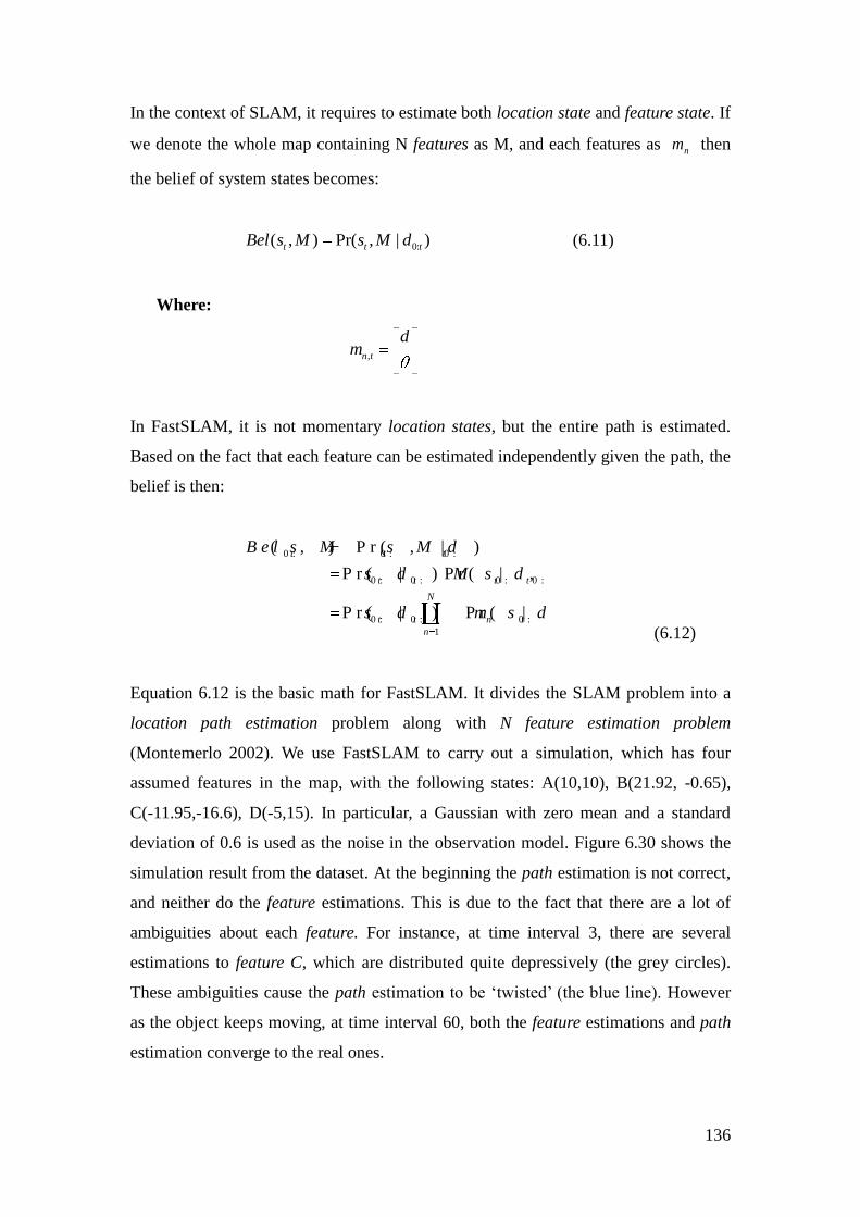
136
In the context of SLAM, it requires to estimate both location state and feature state. If
we denote the whole map containing N features as M, and each features as nm then
the belief of system states becomes:
0:( , ) Pr( , | )t t tBel s M s M d (6.11)
Where:
,n t
dm
In FastSLAM, it is not momentary location states, but the entire path is estimated.
Based on the fact that each feature can be estimated independently given the path, the
belief is then:
0 : 0 : 0 :
0 : 0 : 0 : 0 :
0 : 0 : 0 : 0 :
1
( , ) P r ( , | )
P r ( | ) P r ( | , )
P r ( | ) P r ( | , )
t t t
t t t t
N
t t n t t
n
B e l s M s M d
s d M s d
s d m s d
(6.12)
Equation 6.12 is the basic math for FastSLAM. It divides the SLAM problem into a
location path estimation problem along with N feature estimation problem
(Montemerlo 2002). We use FastSLAM to carry out a simulation, which has four
assumed features in the map, with the following states: A(10,10), B(21.92, -0.65),
C(-11.95,-16.6), D(-5,15). In particular, a Gaussian with zero mean and a standard
deviation of 0.6 is used as the noise in the observation model. Figure 6.30 shows the
simulation result from the dataset. At the beginning the path estimation is not correct,
and neither do the feature estimations. This is due to the fact that there are a lot of
ambiguities about each feature. For instance, at time interval 3, there are several
estimations to feature C, which are distributed quite depressively (the grey circles).
These ambiguities cause the path estimation to be „twisted‟ (the blue line). However
as the object keeps moving, at time interval 60, both the feature estimations and path
estimation converge to the real ones.

137
Figure 6. 30: An simulation result by using FastSLAM with 150 particles:
The black dashed line is the real path (begins from the origin) while the blue line is
the estimated path from the particle filter SLAM algorithm. The square, triangle,
circle and star represent the estimation to feature A, B, C and D respectively. In these
feature estimations the grey ones are the results at time interval 3 while the black ones
are the results at time interval 60. The initialization method for the first observed
feature (here it is feature A) is to pick a random point as its state, hence the estimation
to feature A will remain constant. Also in this experiment feature A is initialized to be
overlapped with its real feature state so that the estimated path will have the same
orientation with the real one.
The above Figure appears that particular filter can potentially be a dynamic
localisation algorithm in an RFID-Loc localisation algorithm. However, there are still
some key barriers on this attempt, which would be discussed and solved in next
section.

138
6.3.2.3 Discussion
The first key barrier of typical Particle Filter localisation algorithms is the high
computational complexity of Particle Filter. Since in localisation, the state space
usually has just 3 or 4 dimensions (e.g. three Cartesian coordinates and possibly one
orientation), while in SLAM the number of features can easily be an order of
hundreds. In order to get a satisfactory result with Particle Filter, the number of
particles needs to rise rapidly with the dimension of the state space (Gordon et.al.
1993). Actually, In FastSLAM, the posterior over location path is estimated by
particle filter, and each particle maintains its own map with N features. These features
are estimated by Extended Kalman Filter (each EKF for one feature) using the same
techniques. Thus if there are M particles, then there will be N×M EKFs in total.
Compared with standard particle filter, far fewer particles are required. And because
each EKF only estimate one single feature, a high-dimensional SLAM problem is
then factorized into a product of low-dimensional estimation problems, which yields a
much improved efficiency. The algorithm used by FastSLAM is actually an
instantiation of the Rao-Blackwellised Particle Filter (Murphy 1999), which uses a
combination of particle representation and parametric representation for a
high-dimensional Bayes estimation problem. For a complete derivation and proof of
this factorization, refer to (Thrun et al 2004). FastSLAM absorbs the advantage of
both Kalman Filter and Particle Filter. As a result it can be applied into highly
non-linear SLAM problems while at the same time maintains efficiency and accuracy.
For the sake of clarity, we carried out some more simulations in Figure 6.31 with
different number of particles, to examine the programming running time and error of
estimation. Figure 6.6 demonstrates the relationship between the number of particles
and the running time of simulation program and the error of estimation. From the
Figure 6.6, it shows that the more number of particles would have a higher accurate
estimation, but with a longer running time. Oppositely, if the number of particles
reduced, it is possible to reduce the running time, but with some loss on accuracy. In
an RFID-Loc system, long running time of localisation algorithm would lead to a time
delay, thus it is necessary to balance running time and error of estimation of Particular
Filter based localisation algorithm.

139
Figure 6. 31: The influence of the number of particles
Secondly, the sensor environment and features of an RFID-Loc system are different
with the typical FastSLAM applications. It is critical to identify their differences so
that we can adopt particular filter technique in an RFID-Loc system. The conventional
FastSLAM particle filters algorithm is to deal with several fixed or unfixed feature
points, which in practical presents the range-measurement sensors, to measure the
distance information at each time intervals. The observation is distance information.
However, in an RFID-Loc system, features are extracted by RFID-Loc data filter,
which are position information. The impacts of features on object position are not
equal. In a conventional FastSLAM algorithm, features would impact on localisation
of both X axis and Y axis of moving object. In an RFID-Loc system, two features on
X axis impacts on X value of object position, another two features on Y axis impacts
on Y value of object position. Considering those differences on sensor environment
and features, FastSLAM particle filter algorithm cannot be directly applied into an
RFID-Loc system. The aim of FastSLAM is to accurately localize the mobile object
by using range sensor with the environment of unknown start position and feature
position. It contains the feature based estimation for mapping and localisation. But in
an RFID-Loc system, although the features extracted by RFID-Loc data filter have
some uncertainty and errors, the mapping between features and object position is clear
and explicit. Strictly speaking, dynamic localisation process for an RFID-Loc system
is solely a localisation process without mapping process. In light of those differences
between RFID-Loc environment and typical FastSLAM applications, it is necessary
to propose a new particle filter based localisation algorithm for an RFID-Loc system.
In a typical FastSLAM algorithm, by using the observation model and motion model,
it would estimate the position information of moving object. The whole localisation

140
process contains initializing, applying model, weighting, and resampling. It can use
some range-only measurement sensors in that for mobile objects localisation, and
most sensors are easily to observe the distance information rather than position
information. As for an RFID-Loc application, dynamic localisation process can also
contain initializing, applying model, weighting and resampling process. However,
since RFID reader observes position value of RFID tags instead of distance value, the
proposed dynamic localisation algorithm would rebuild different observation model,
motion model, and define feature points, weighting process, resampling process. The
comparison of a proposed dynamical localisation approach and conventional
FastSLAM approach is shown in Table 6.6.
Table 6. 6 Comparison of RFID-Loc Dynamic Localisation and SLAM
RFID-Loc Dynamic Localisation FASTSLAM
Feature points
Position information, Mobile.
Distance information, Nearly fixed.
Initialization Known start position, Known start features.
Unknown start position, Unknown start features position.
Sensor Data Position information
Distance information
Applying motion model
Gaussian model, but the radius is determined by known accuracy ( tag distance )
Gaussian model, the radius could be any value.
Observation model and weighting
Observation model is based on the position difference between predicted value and observed value.
Observation model is based on the distance difference between predicted value and observed value.
Feature Impacts
Two features on X axis impacts on output X value, another two features on Y axis impacts on output Y value.
Four features impacts on both output X and Y value.
Resampling Directly use the particles with largest weight.
Those particles with large weight will be duplicated while those with small weight will be deleted.
Aim Accurately localize the object by using position sensor with the environment of known start position and feature position.
Accurately localize the mobile object by using range sensor with the environment of unknown start position and feature position.
Performance No strict convergence, the accuracy at each time interval is only determined by the closeness of predicted features to observation features.
With increasing time intervals, the position has a convergence with high accuracy.

141
6.3.3 System State and Model Definitions
In this section, it proposes a new particle filter based dynamic localisation algorithm
for an RFID-Loc system. This section provides a comprehensive description of the
implementation of system states, system models and the particle filter in this
algorithm.
6.3.3.1 System state
Hence all features as well as the location of the object can be represented by Cartesian
coordinates. The chosen four feature points ynypxnxp
FFFF ,,, are the minimum and
maximum values on X and Y axis among all the detected RFID tag position value at
time interval t, as shown in Equation 5.1 in Chapter 5. If current time interval is
denoted as t, object position ),( c
t
c
tYX
can be obtained through the position data of
RFID tags ( , )N N
T TX Y , where N represents the number of tags detected by the reader,
and ( , )N N
T TX Y represents the coordination information of the tags. Then the chosen
feature points are represented in the following Equation 6.13
1 2
1 2
1 2
1 2
( , ,...... )
( , ,...... )
( , , , )
( , ,...... )
( , ,...... )
N
xp t t t
N
xn t t t
N
yp t t t
N
yn t t t
F Max x x x
F Min x x x
F xp xn yp yn
F Max y y y
F Min y y y
Feature State (6.13)
After defining the state of four feature points, it requires to define a system state to
represent the localisation process. The location state represents the position of object,
is defined as S in Equation 6.14, where n is index of feature points, t is the time
interval.
( , )t t tS x y Location state (6.14)

142
Having defined the feature states and location states, the system state, at time t, the
system state t
ST is shown as Equation 6.15:
t
xp
t
xnt t
yp
t
yn
t
s
F
ST F
F
F
System State (6.15)
Given the above overview of system state, the specific objective of this dynamic
localisation algorithm is : the object starts moving from an initial position 0
S with
prior knowledge of the feature points:0 0 0 0, , ,xp xn yp ynF F F F . As the object keeps moving
it receives different features‟ data from the RFID readers. The value of feature points
would change as the object moving.
6.3.3.2 System models
Besides system states, there are two models that need to be defined, namely the
observation model and motion model. Their specific implementation is characterized
by the nature of the RFID sensor system and the motion of object moving.
The observation model tells the probability of obtaining a object position at a certain
location state. Recalling the theory of Bayes Filter, this is defined as a probabilistic
distribution:
)|),,,(P r ( tt SypynxpxnF
Where: ),,,( ypynxpxnFt and
tS are the RFID reading and location state,
respectively.

143
Unlike most other SLAM problems in literature that uses range-bearing sensors. The
characteristic of RFID reader is that it can only provide relative position information,
but not distance or bearing information. This will bring a lot of differences on the
initialization and observation process in the proposed dynamic localisation. Also
RFID tag position information will contain some noise which is caused by
environment. Therefore, the straight observation model would be in Equation 6.16:
x p x p
t t
xn xn
t t
yp yp
t t
yn yn
t t
d F
d F
d F
d F
(6.16)
Where: , , ,xp xn yp yn
t t t td d d d are the observations of features at time interval t.
is the noise of measurement each time interval.
At each time interval, RFID reader will receive observation information from all
features. Figure 6.32 is an example showing an RFID-Loc system measuring the
position information from four features at the same time. While in practice, RFID
reader may receive observation of each RFID tag one by one, a time gap is given to
collect enough RFID raw data, etc, 20 seconds in Chapter 4 case. And then the four
features can be treated as simultaneously extracting from RFID raw data.

144
( )tF yp
( )tF xn
( )tF xp
( )tF yn
Figure 6. 32: The Observation Model
The straight observation model gives the relationship between the object position and
the features value. But it is not enough as we need another model which can provide
the feature states given the location state of the object and the observation information.
The inverse observation model offers such functionality.
The motion model is used to characterize the moving object location states over time.
It helps to predict the next moving object location state given the most current one. In
a real indoor environment, moving object is possibly human carrying or wheel driving.
Moving object might change its direction or speed of the movement randomly. So the
targeted moving object trajectory is assumed to be associated with direction or speed
of the movement that is random. To cope with the randomness of the motion moving,
a 2D Gaussian model is used to approximate the motion. More specifically, when
given the location state t
S at the time interval t, to predict the location state at
the time t+1, a number of particles are drawn randomly from a 2D Gaussian
distribution with zero-mean. These particles will be distributed in a circle with origin
at t
S and its radius is determined by the standard deviation of the 2D Gaussian
distribution. For instance, if moving object position start from position (0, 0), and
localisation accuracy in a RFID-Loc system would reach 5 centimeters, so the next
step of position possibly is on the circle which is on the centre (0,0), with the radius
2*5 , and draw 200 particles, the diagram is shown in Fig 6.33

145
Figure 6. 33: The Motion Model
Figure 6.33 shows an example of the motion model using 200 particles. Notice that in
practice it is not necessary to use so many particles. Usually around 100 particles are
enough to obtain satisfactory results. But using more particles can improve the
accuracy for the estimation of location states.
The main advantage of using a 2D Gaussian to approximate the motion model is its
ability to cover all possible motion directions. In order to predict location state
accurately, the standard deviation of this 2D Gaussian has to be carefully specified.
However, this motion model also has two limitations which may significantly affect
the efficiency of the dynamic localisation algorithm in certain circumstances. The first
problem arises because it simply draws particles from a 2D Gaussian randomly and
consequently there will be some particles being “wasted” since they may be placed at
positions with low observation likelihood. The other drawback is a direct consequence
of the particle-wasting problem. If the total number of the particle is not big enough
then there will be too few particles placed at the high observation likelihood area and
therefore the prediction accuracy will be significantly affected. There two problems
are from the nature of the resampling process of standard particle filter and have been

146
broadly recognized by researchers. In order to overcome this problem, we would
employ a simple method, which only select the biggest weight particle for generating
the location states.
6.3.4 Dynamic Localisation Algorithm for RFID-Loc
After defining the system state and observation model, it requires clearing the
structure of each particle. The conventional particle filter structure only contains the
localisation state and feature states without including weight issues. But in this
algorithm, we would put the weight state into particle state. Each particle has a
mathematical way in Equation 6.17.
, , , , , , , ,
{ , , , , , , , , , }M M M M M M M M M M M
t t x p t x n t y p t y n t x p t x n t y p t y n t tS T S F F F F W W W W U (6.17)
Where:
M is the index of the particle,
t is the time interval.
m
ts is the location of the object
m
tnf , represents feature points.
M
tnW
, represents the weight of each feature.
M
tU is the updated location of object.
The particle filter algorithm is then operating on a set of particles. Each iteration of
the algorithm can be divided into the following stages:
(a) Initialization:
(b) Applying motion model:
(c) Apply observation model and weight all the particles
(d) Resampling
Note that the initialization stage is required only one in the first iteration.

147
6.3.4.1 Initialization
Initialization is an important stage in all conventional SLAM algorithms. In EFK
based SLAM, its task is to initialize the mean and covariance matrix for the state
vector. In the typical particle filter algorithm, it is to initialize the location state and
feature states in each particle. Most of times, the start position of target and features
are unknown, so that the errors at the beginning stage is big. However, in RFID-Loc
case, the RFID sensor could provide the position information initially; it could start at
a known position and feature points. Hence, according to the theoretical model, the
start position is zero, radius as the accuracy of localisation required, feature points
position are calculated as the RFID reader detection area. (Length as Y axis, Width as
X axis).
)0,0(0
S , Accuracy r , 10,
M
nW
)(0,1
Ln e a rf m , )(0,2
Wnearf m , )(0,3
Lnearf m , )(0,4
Wnearf m
Initialization (6.18)
Where : Near () : the nearest tag in the RFID reader detection edge area
6.3.4.2 Applying Model and Weighting
After the initialization, the motion model is applied to all particles. More specifically,
the location state of each particle will be replaced with a new predicted one generated
from the motion model, and the predicted feature state of each particle will be updated
as well. The process is as followed:
At the time intervals t : Once applying motion model to Equation 6.9, the M particles
get M numbers of different predicted position state M
tS
1, which are allocated in the
circle of centre point M
tS , radius as Accuracy
1P r e d i c t _ M o t i o n _ M o d e l ( )M M
t tS S (6.19)

148
Then due to the known RFID reader detection area, it could estimate the position of
predicted features:
, 1 1P r e d i c t _ P r e d i c t _ ( )M M
xp t tF S near W
, 1 1P r e d i c t _ P r e d i c t _ ( )M M
xn t tF S near W
, 1 1P r e d i c t _ P r e d i c t _ ( )M M
yp t tF S near L
, 1 1P r e d i c t _ P r e d i c t _ ( )M M
yn t tF S near L (6.20)
Here, each particle has its estimation to the location state and feature states. Then we
define predicted location state as the location state after being applied the motion
model. And define predicted observation as the features‟ value. Then the weight of
each particle should be determine by the difference of the predicted observation and
real observation. If the predicted location state and feature state is very close to the
real states. Then the predicted observation will be very close to the real observation.
Hence this particle will have a high weight. In a probabilistic math form, the weight
of each particle is given by:
0 : 1 0 : 1P r ( | , ) P r ( | , )m m m
t n t n t t nW d f s f s d d f (6.21)
Where the superscript m is the index of the particle, subscript t is time interval,
Equation 6.21 is implemented by calculating the real observation under a Gaussian
with mean and standard deviation determined by the observation noise. More
specifically, the weight of each particle is calculated using the following Equation
6.22. Meanwhile, it already got the four predicted feature points value at time
intervals 1t , it could apply the observation model by using the observed feature
points date to calculate the weight of each particles.

149
2( P r e d i c t _ ), 1 1
22 1/2 2, 1
2(Predict _ ), 1 1
22 1/2 2, 1
2(Predict _ ), 1 1
22 1/2 2, 1
2(Predict _ ), 1 1
22 1/2 2, 1
(2 )
(2 )
(2 )
(2 )
xpMF dxp t t
M
xp t
M xnF dxn t t
M
xn t
ypMF dyp t t
M
yp t
ynMF dyn t t
M
yn t
W e
W e
W e
W e
(6.22)
Currently, it already got all the weights, the next stage is to use these weights and get
the update object position.
6.3.4.3 Resampling
This step is similar as the one in particle filter localisation. In a conventional particle
filter localisation process, those particles with large weight will be duplicated while
those with small weight will be deleted. And all the weight would accumulate to
impact on the position value. However, in this dynamic algorithm, the situation varies
the traditional one in that the four features weight would separately influence the X
and Y axis value by two parts, which is that M
txpW
1, and M
txnW
1,would determine the X
position value, M
typW
1, and M
tynW
1, would determine the Y position value.
Consequently, it would pick up the largest weight to calculate the updated object
position, since it means that the possibility of object position at that predicted location
is the largest. If it is denoted the particle number of largest weight on X positive, X
negative, Y positive and Y negative directions are _i xp , _i xn , _i yp , _i yn ,
then

150
1 2
, 1 , 1 , 1
1 2
, 1 , 1 , 1
1 2
, 1 , 1 , 1
1 2
, 1 , 1 , 1
_ _ ( , ,..., )
_ _ ( , ,..., )
_ _ ( , ,..., )
_ _ ( , ,..., )
M
xp t xp t xp t
M
xn t xn t xn t
M
yp t yp t yp t
M
yn t yn t yn t
i xp Max index W W W
i xn Max index W W W
i yp Max index W W W
i yn Max index W W W
(6.23)
The updated moving object position M
tU
1 could be the next step moving object
position state M
tS
2, and the algorithm would continue running to estimate the moving
object position.
_ _ _ _
1 1 1 11
Predict _ Predict _ Predict _ Predict _,
2 2
i xp i xn i yp i ynM t t t tt
S S S SU (6.24)
6.3.5 Algorithm Summary
This section will provide a summary of the whole dynamic localisation algorithm for
RFID-Loc, as shown in Figure 6.34:

151
Figure 6. 34: Dynamic Localisation Algorithm Flow Chart

152
6.4 Summary
In this chapter, how to filter RFID raw data and select reliable features and process
these features to localize object position in RFID-Loc are discussed. Under a given
RFID-Loc infrastructure platform, experiment results showed that regular false
negative reading is the most frequently occurring factor affecting to inaccuracy and
uncertainty of RFID raw data. Points based, polygon based and rectangle based
feature selection methods are compared by evaluating accuracy and precision of an
RFID-Loc system in three different trajectories. The comparison explores that by
using centroid localisation algorithm, rectangle based feature selection method can
give higher localisation precision than points and polygon based feature selection
method, particularly on X axis value of object position. It means that rectangle based
feature selection method can maximum reduce the impacts of regular false reading
error on localisation precision from software level, because rectangle area substituting
a polygon area in a feature selection method can solve the problem of asymmetry of
features in RFID raw data. While under proposed RFID-Loc infrastructure and feature
selection method, static localisation algorithm in an RFID-Loc system can localize the
object position with a good accuracy. But static localisation algorithm has a weak
ability to resist unexpected false reading error in an RFID-Loc system. Analysis
shows that RFID-Loc is a simpler case than typical SLAM problem, but with much
difference. A dynamic localisation algorithm based on particle filter technique is
proposed and implemented to solve the problem of resisting unexpected false reading
error in an RFID-Loc system, particularly on dead reading error and repeated
reading error. Experiments showed that dynamic localisation algorithm has a similar
accuracy and precision to static localisation algorithm in regular false reading error
occurring situation, and a better precision than static localisation algorithm in
unexpected false reading error occurring situation. The robustness of proposed
dynamic localisation algorithm has to depend on the chosen number of particles and
initial distributed radius.

153
Chapter 7:
Results Analysis and Discussion
7.1 Introduction
In this Chapter, the application of RFID-Loc framework is discussed, verifying its
potential use for indoor application, and providing examples of how it can be used in
different scenarios. In order to verify the framework, several experiments with
different object moving trajectories are carried out. Section 7.2 focuses on the
validation of proposed spare RFID Tag Arrangement Strategy on improving
localisation precision by comparing with conventional grid RFID Tag Arrangement.
Section 7.3 verifies the performance of proposed dynamic localisation algorithm on
resisting false-reading error. Section 7.4 illustrates the whole performance of an
RFID-Loc based system by using proposed RFID infrastructure and algorithms on
localisation accuracy and precision, with comparison to some traditional RFID based
localisation systems.
7.2 Validation of Sparse RFID Tag Arrangement
Strategy
To evaluate the validity of proposed sparse RFID Tag Arrangement strategy for an
RFID-Loc system, the direct way is to check how much improvement on system
reading efficiency of RFID-Loc Infrastructure module. Comparing RFID tag pattern
in Figure 5.18 and 5.3, M has reduced from 28 to 18, as shown in Figure 7.1.

154
Conventional Grid Tag Pattern Spare Tag Arrangement Pattern
Figure 7. 1 Comparison of two RFID Tag Arrangement patterns
In terms of Equation 4.6, under given experimental platform, system reading
efficiency of RFID-Loc infrastructure has increased from 30% to 40%, which means
that proposed sparse RFID Tag Arrangement strategy can reduce regular false reading
error in an RFID-Loc system.
Apart from evaluating system reading efficiency, as mentioned in section 4.4, it would
also focus on evaluating localisation accuracy and precision with the proposed sparse
RFID Tag Arrangement on some object moving trajectories. In both two patterns of
Figure 7.1, accuracy is given as up to 10 centimetres, then:
10x y
D D cm
So in practical experiment process, the distance of object moving between two time
intervals is equal to this accuracy, which is 10 centimetres. The testing trajectories are
to move along X axis, move along Y axis and move along both X and Y axis. Time
interval of localisation sequence is measured by 12. Localisation algorithm for
calculating object position is to use Equation 4.3. The experimental results of object
moving along X axis, Y axis, both X and Y axis, are shown in Figure 7.2, 7.3 and 7.4.

155
These three Figures illustrate that sparse RFID Tag Arrangement can give a better
localisation performance than original RFID grid Tag Arrangement. This phenomenon
occurs apparently on object moving along X axis. While on object moving along Y
axis, new sparse RFID pattern cannot give an apparently improved localisation
performance than original RFID grid pattern, it reduced localisation precision on
some time interval in original RFID grid pattern. As for object moving along both X
and Y axis, original RFID grid pattern produces some significant errors on some time
intervals, but new sparse RFID pattern gives a roughly better performance than grid
one.
Figure 7. 2 RFID sensing trajectory along X axis.

156
Figure 7. 3 RFID sensing trajectory along Y axis.
Figure 7. 4 RFID sensing trajectory along both X axis and Y axis.

157
In terms of the above three trajectories, localisation accuracy and precision of new
sparse RFID pattern and traditional RFID grid pattern are compared in Table 7.1.
Also, value of localisation precision over 12 time intervals is averaged into Figure 7.5.
By using new sparse RFID pattern, the range of localisation precision has been
reduced from 10 centimetres level to 5 centimetres level.
Table 7. 1 Comparison of Accuracy and Precision Range on two RFID tag patterns
X Axis
Trajectory
Y Axis
Trajectory
X and Y
Trajectory
Accuracy
Grid
Pattern
X and Y value
of position
10cm
10cm
10cm
New
Pattern
X and Y value of
position
10cm 10cm 10cm
Precision
Grid
Pattern
X value of
position
(-8,10) cm (-10,12)cm (-11,10) cm
Y value of
position
(-5,7) cm
(-6,11) cm
(-8,12) cm
New
Pattern
X value of
position
(-5,5) cm
(-4,4.5) cm
(-5,4) cm
Y value of
Position
(-3,2) cm
(-5,4) cm
(-4.5,5) cm
Figure 7.5 shows that average localisation precision in continues time intervals has
also reduced from 10 centimetres to 3 centimetres. So it indicates that compared to
original RFID grid tag pattern, sparse RFID tag pattern can significantly improve the
performance of RFID-Loc based object localisation system. While the improvement
on objective position X and Y is with different degree, comparing to the localisation
performance of original grid tag pattern, localisation precision of object moving along
three different trajectories can enhance nearly 50% with the proposed sparse RFID
pattern. As for localisation accuracy, tag distance between those two patterns is
equivalent to 10 centimetres, so it means that localisation accuracy is unchanged. To
the end, the proposed new sparse RFID Tag Arrangement strategy is superior to the
current RFID Tag Arrangement method in terms of precision.

158
Figure 7. 5 Comparison of Average Precision on two RFID Tag Patterns
7.3 Validation of Dynamic Localisation
Algorithm
A number of experiments have been carried out, using different datasets, different
numbers of particles and other various settings. These experiments are to evaluate the
performance of particle filter based dynamic localisation algorithm on resisting to
false reading error, and to investigate if this algorithm has been successfully
implemented for 2D position estimation and localisation in a RFID-Loc system in
terms of accuracy, precision and robustness. The datasets in these experiments are
similarly collected from last section, which includes three object moving trajectories
along X axis, Y axis and Random motion. Hence, the parameters in these experiments
are the same as previous chapters.

159
7.3.1 Regular False Reading Error
To begin with, it compares localisation performance of proposed dynamic localisation
algorithm with static localisation algorithm on accuracy and precision, with the same
extracted features. Moving distance of object at each time interval is 10 centimetres,
which is equal to the assumed localisation accuracy. The radius of circle for
distributing particles is initialized as 20 centimetres, so that it can potentially cover all
possible moving directions and positions. As for start position, since every dataset
started from different position, different ones are selected as start position. The
number of particles would be assumed as 100 at the beginning.
Figure 7.6 and Figure 7.7 shows that the performance of static and dynamic
localisation algorithm on the situation that object only moving along X axis. The start
position is (0,-2).
Figure 7.8 and Figure 7.9 shows that the performance of static and dynamic
localisation algorithm on the situation that object only moving along Y axis. The start
position is (0,-2).
Figure 7.10 and Figure 7.11 shows that the performance of static and dynamic
localisation algorithm on the situation that object only moving along a random
trajectory. The start position is (0,-2).

160
Figure 7. 6 Comparison on X Trajectory
(b) Error on X axis (b) Error on Y axis
Figure 7. 7 Errors Comparison on X Trajectory

161
Figure 7. 8 Comparison on Y Trajectory
(a) Error on X axis (b) Error on Y axis
Figure 7. 9 Errors Comparison on Y Trajectory

162
Figure 7. 10 Comparison on Random Trajectory
(a) Error on X axis (b) Error on Y axis
Figure 7. 11 Errors Comparison on Random Trajectory

163
From the above Figures, X and Y trajectory represent that dynamic localisation
algorithm can get a roughly identical accuracy as static localisation algorithm on
those two cases. However, in this situation of random trajectory, dynamic localisation
algorithm generates a bigger error than static localisation algorithm. Theoretically,
random trajectory can be viewed as a combination of many small moving segments
on X axis or Y axis. Consequently, if dynamic localisation algorithm can be effective
on those two cases, it would be also effective on random moving trajectory. The
possible reason leading to bigger error of dynamic localisation algorithm is the length
of radius to distribute the particles. If length of radius is not long enough, the particles
in the circle would be impossible to cover all possible moving directions and positions
at next step. In order to explore the impact of the length of radius on the performance
of dynamic localisation algorithm, the length of radius is selected and evaluated by 30
centimetres, Figure 7.12 and 7.13 shows algorithm performance on random trajectory.
Figure 7. 12 Radius at 30 centimetres on Random Trajectory

164
(b) Error on X axis (b) Error on Y axis
Figure 7. 13 Comparison Errors on Random Trajectory (Radius 30 centimetres)
To summary above localisation precision by using similar criteria in section 5.4.4,
accuracy has already given as 10 centimetres; precision can be compared by mean of
precision in Table 7.2 and range of precision in Table 7.3. The mean of precision can
be calculated by Standard Deviation.
Table 7. 2 Comparison of Feature Selection Methods by mean of precision
Methods X Trajectory
X value Y value
Y Trajectory
X value Y value Random Trajectory
X value Y value
Static 6.686 cm 5.353 cm 3. 356 cm 7. 854 cm 0. 289 cm 7. 220 cm
Dynamic 5.427 cm 6. 075 cm 0. 905 cm 8. 891 cm 0. 481 cm 9. 936 cm
Table 7. 3 Comparison of Feature Selection Methods by range of precision
Methods X Trajectory
X value Y value
Y Trajectory
X value Y value Random Trajectory
X value Y value
Static (-2.8, 9) cm (-13, 1) cm (-3, 8.3) cm (-10, 16.7)
cm
(-6.7, 5) cm (0, 13) cm
Dynamic (-5, 4.5) cm (-5, 1.5) cm (-5, 5) cm (-5, 25) cm (-5, 5) cm (3, 25) cm
It appears that as the increased length of radius, dynamic localisation algorithm can
work effectively on a random trajectory. Also it can reach approximately same
localisation accuracy as static localisation algorithm. Therefore, it shows that with the
selected suitable radius and start position, the proposed dynamic localisation
algorithm can have a similar localisation performance with static localisation
algorithm.

165
7.3.2 Unexpected False Reading Error
This section compares the performance of proposed dynamic localisation algorithm
with static localisation algorithm on dealing with unexpected false reading error
situations. Dead reading error and repeated reading error are mainly tested since they
are serious and typical in unexpected false reading error. Those two kinds of
unexpected false reading error can possible occur discretely and continuously.
Therefore, it would evaluate the proposed dynamic localisation algorithm
performance on those four situations. The results of the proposed dynamic localisation
algorithm with the conventional static localisation algorithm are compared. The
dataset is from a object moving trajectory including moving along X axis, moving
along Y axis and moving random directions.
a) Discrete dead reading error
On this condition, it assumed that dead reading error discretely occurs at the time
interval 10, 20, 30; start position (-8.5, -3.5), radius length 30 centimeters. Figure 7.14
and 6.19 shows the error of estimated value along X axis and Y axis between dynamic
and static algorithm and real simulated object moving path.
Figure 7. 14: Dynamic algorithm localisation performance on discrete dead-reading

166
(a) Error on X axis (b) Error on Y axis
Figure 7. 15 Errors Comparison on discrete dead reading error
In comparison to conventional static localisation algorithm, dynamic localisation
algorithm can effectively improve localisation precision on discrete dead reading error
situations. It is because particle filter based dynamic localisation algorithm has limited
the possible object position in a circle with radius 30 centimetres, so that the possible
localisation errors would also be limited in this range. Once RFID reader observes the
new features, dynamic localisation algorithm can recover object position immediately.
b) Continuous dead reading error
On this condition, it assumed that the dead reading error continuously occurs at the
three time interval 5,6,7; 15,16,17; 25,26,27; start position (-8.5, -3.5), radius length
30 centimetres. Fig 7.16 and 7.17 shows the error of estimated value along X axis and
Y axis between dynamic and static algorithm and real simulated object moving path.

167
Figure 7. 16 Dynamic algorithm localisation performance on continuous dead reading
error
(a) Error on X axis (b) Error on Y axis
Figure 7. 17 Errors Comparison on continuous dead reading error in three time
intervals
During the three time intervals, it appears that in comparison to the conventional static
localisation algorithm for RFID-Loc, dynamic localisation algorithm can effectively
improve localisation accuracy on continuous dead reading error situations. However,

168
the period of three continuous time intervals can not represent all the possible
situations of continuous dead reading error, thus the time intervals are extended to 5
and 7, then to see their performance, as shown in Figure 7.18 and Figure 7.19. The
results show that dynamic localisation algorithm can still effectively recover the
object position from continuous dead reading error situation. The proposed dynamic
localisation algorithm is better to deal with continuous dead reading error situations
than static localisation algorithm for an RFID-Loc system.
(a) Error on X axis (b) Error on Y axis
Figure 7. 18 Errors Comparison on continuous dead reading error in five time
intervals
(a) Error on X axis (b) Error on Y axis
Figure 7. 19 Errors Comparison on continuous dead reading error in seven time
intervals

169
c) Discrete repeated reading error
On this condition, it assumed that repeated reading error discretely occurs at the time
interval 8, 17, 27; start position (-8.5, -3.5), radius length 30 centimetres. Figure 7.20
shows the error of estimated value along X axis and Y axis between dynamic and
static algorithm and real simulated object moving path.
(b) Error on X axis (b) Error on Y axis
Figure 7. 20 Comparison Errors on discrete repeated readings error situation
In comparison to conventional static localisation algorithm, dynamic localisation
algorithm can have a roughly identical localisation performance on discrete repeated
reading error situation. It is because on discrete repeated reading error situation,
RFID reader practically observes some RFID raw data, only with the same value with
previous time interval. On this condition, if the length of radius is enough to cover the
object position of previous time interval, dynamic localisation algorithm would
generate the same object position as static localisation algorithm at this time interval.
However, due to the limited length of radius, the estimated object position on next
time interval might have some errors.

170
d) Continuous repeated reading error
On this condition, it assumed that repeated reading errors continuously occur at the
four continuous time intervals 8,9,10,11; 17,18,19,20; 27,28,29,30; start position (-8.5,
-3.5), radius length 30 centimetres. Figure 7.21 shows the error of estimated value
along X axis and Y axis between dynamic and static algorithm and real simulated
object moving path.
(c) Error on X axis (b) Error on Y axis
Figure 7. 21 Errors Comparison on continuous repeated reading errors in three time
intervals.
From the results, it appears that the in comparison to conventional static localisation
algorithm, dynamic localisation algorithm can effectively improve localisation
precision on continuous repeated reading errors situations, especially on X axis.
To summarize four situations, dynamic localisation algorithm has a better
performance on dealing with unexpected false readings error than conventional static
localisation algorithm for an RFID-Loc system. The primary reason is that dynamic
localisation algorithm is based on particle filter methods, which has a strong ability to
recover the errors in localisation process. Secondly, dynamic localisation algorithm
seems to be more efficient on dealing with continuous situations than static
localisation algorithm, subject to a proper length of radius for distributing particles.

171
The reason is that dynamic localisation algorithm has the predicted and updated
processes to connect continuous time intervals, but static localisation algorithm just
has the individual processes on each discrete time interval.
7.3.3 Robustness of Algorithm
Although the proposed particle filter based dynamic localisation algorithm illustrates
a better localisation performance than static localisation algorithm in an RFID-Loc
system, the robustness of algorithm is still of importance to be concerned. There are
two factors impacting the robustness of algorithm, the number of particles and the
length of radius for distributing particles. Typically, as the increased number of
particles, the localisation accuracy would be increased. If the environment is more
complex, it required more particles, which cost much time on calculation. Thus, it is
necessary to know how to choose the number of particles; the number of particles is
chosen as 20, 50, 100, 200, 400, 800 to evaluate the robustness of algorithm, and the
error of X and Y are standard mean. Meanwhile, due to the randomness of distributing
particles, dynamic localisation algorithm would perform differently on varied
distributions, so it requires running several times for comparing the difference. Table
7.4 and 7.5 separately show the results of dynamic localisation algorithm dealing with
continuous dead-reading (5 time intervals) and discrete dead-reading situations.
Table 7. 4 Standard Error Mean of Different Number of particles on Continuous
Dead-Readings
Times Standard
Error
mean
20
Particles
50
Particles
100
Particles
200
Particles
400
Particles
800
Particles
1 X
Y
5.7183
2.836
3.3887
11.021
1.6898
2.2502
2.1545
1.6887
2.4313
2.9541
4.9051
2.5636
2 X
Y
4.9873
2.5292
3.36019
3.0219
2.453
8.5965
2.802
1.9256
5.6722
2.6206
3.4605
2.4889
3 X
Y
3.6204
10.7526
6.0376
8.9907
3.6389
1.3014
5.0026
5.0975
1.9846
5.084
4.0788
2.6942
4 X
Y
12.0856
7.9734
1.5671
2.0616
4.4719
2.2836
4.6668
2.3384
3.5893
8.8096
6.0933
8.3007
5 X
Y
3.5373
2.7631
2.6858
1.9723
2.3562
1.0283
3.6663
9.5804
1.5968
1.5888
4.5654
1.8237
6 X
Y
1.1449
2.9168
5.2231
3.4289
3.8413
5.085
1.5196
2.4062
2.2598
12.777
4.3468
5.1622

172
Table 7. 5 Standard Error Mean of Different Number of particles on Discrete
Dead-Readings
Times Standard
Error
mean
20
Particles
50
Particles
100
Particles
200
Particles
400
Particles
800
Particles
1 X
Y
0.8502
1.2817
0.977
1.7064
0.5762
1.2179
0.6822
1.0008
0.6785
1.4473
0.5763
1.3841
2 X
Y
0.8007
1.1405
0.6684
0.673
0.6878
2.128
0.7143
0.9541
0.6311
0.8065
0.9676
1.0483
3 X
Y
1.0815
1.8567
0.5442
0.7462
0.7579
0.7229
0.6893
1.3223
0.6574
2.0474
1.0388
1.0099
4 X
Y
0.9568
0.7068
0.5292
1.8899
0.4966
1.1677
0.5508
1.1504
0.5836
2.1328
0.6297
0.8928
5 X
Y
0.7079
1.1872
0.616
1.208
1.0103
1.0125
0.6045
0.8271
0.7037
1.0106
0.5608
1.9764
6 X
Y
0.6959
1.5173
0.5874
1.5643
0.6139
1.0058
0.5555
0.9411
0.561
1.8575
0.614
1.0434
The above Tables show that random distribution of particles would lead to varied
standard error mean, even with the equal number of particles. So we would average
the error value in the above Tables, and draw the trend in Figure 7.22 and 7.23.
Figure 7. 22 Different number of Particles on continuous dead reading error situation

173
Figure 7. 23 Different number of particles on discrete dead reading error situation
From above two Figures, it shows that as the number of particles increase, the error of
dynamic localisation algorithm would initially decrease, but then increase again. The
reason is that the performance of dynamic localisation algorithm depends on the
distribution of particles to a large extend. If the number of particles is small, the
density of distributing particle area is very low, so as to the high probability of object
position might not be covered. Oppositely, if the number of particle is large, the
density of distributing particle area is high, although the high probability of object
position is covered; the probability of covering unexpected false readings position is
also increased. Consequently, on the condition of unexpected false reading error
occurring, dynamic-localisation algorithm with a large number of particles would also
be possible to generate big error. Therefore, the ideal number of particles in this case
is between 100 and 200. With this number, the particle can be distributed fairly.

174
7.4 Validation RFID-Loc Solution
This section considers verifying the RFID-Loc framework with both proposed RFID
Tag Arrangement and localisation algorithm to localize the moving object in a basic
and simple indoor environment as a case study.
The first issue needs to be verified is the predictive capacity on accuracy and
precision of an RFID-Loc framework by using proposed RFID infrastructure and
algorithms. The traditional passive RFID tags based localisation system relies on
highly dense grid tag pattern and static localisation algorithms. RFID-Loc framework
in this thesis has provided an optimal RFID button tag arrangement pattern, a
rectangle based feature selection method and a dynamical particle filter based
localisation algorithm. The accuracy and precision delivered by proposed RFID-Loc
framework has to be compared with the accuracy and precision of traditional RFID
based localisation system, to see if it has a better performance than traditional RFID
based localisation system.
Secondly, moving speed of object has to be concerned in an indoor environment. In
this thesis, Chapter 2 has reviewed that in a dense RFID tag environment, RFID
reader needs a sufficient response time to observe a basically enough RFID data for
processing. On this case, the time period of object keeping on one step T, which is
defined in Chapter 4, is more important than object moving speed to accuracy and
precision delivered by an RFID-Loc framework. Therefore, the experiment also has to
verify the impacts of different value of T on the accuracy and precision delivered by a
localisation solution based on RFID-Loc framework.
7.4.1 Localisation Accuracy and Precision
For verifying the predictive capacity on accuracy and precision of an RFID-Loc
framework by using proposed RFID infrastructure and algorithms, two typical passive
RFID based localisation solutions are compared. The typical RFID localisation
solution is based a regular grid passive RFID tag pattern, as shown in Figure 7.24.
Localisation algorithm in this solution is usually a simple average method in Equation

175
4.7 in Chapter 4. The second RFID-Loc localisation solution is based a triangular
passive RFID tag pattern, as shown in Figure 7.25. Localisation algorithm in this
solution is usually a simple average method in Equation 4.8 in Chapter 4. The
proposed RFID-Loc based localisation system is to use a sparse RFID tag pattern, as
shown in Figure 7.26. The localisation algorithm is to use the methods proposed in
Chapter 6.
Figure 7. 24 Grid based passive RFID localisation solution

176
Figure 7. 25 Triangle based passive RFID localisation solution
Figure 7. 26 Sparse RFID tag pattern delivered by an RFID-Loc framework

177
Of above three patterns, RFID tag distance is already assumed as 10 centimetres, thus
localisation accuracy in the above three solution would be identical. As for
localisation precision, these three solutions are validated into two typical objects
moving trajectories in an indoor environment, which are Truck (along X axis), Dolly
(along Y axis). In each experiment, time intervals of object moving are assumed as 50,
which is larger than the assumed time intervals in Chapter 6. Standard Error of Mean
is adapted to measure localisation precision, by Equation 5.6 in Chapter 5.
Table 7. 6 Comparison by mean of localisation precision
Methods RFID-Loc Solution Error on X Error on Y
Grid Solution Error on X Error on Y
Triangle Solution Error on X Error on Y
Truck Movement
0.92 cm 4.35 cm 6.95 cm 5.63 cm 8.15 cm 6.68 cm
Dolly Movement
2.23 cm 2.38 cm 3.42 cm 7.63 cm 4.12 cm 8.36 cm
Table 7. 7 Comparison by range of localisation precision
Methods RFID-Loc Solution Error on X Error on Y
Grid Solution Error on X Error on Y
Triangle Solution Error on X Error on Y
Truck Movement
(-5,10) cm (4,5) cm (-3,9) cm (-14,2) cm (-5,10) cm (0, 8) cm
Dolly Movement
(-5,10) cm (-10,5) cm (-4,9) cm (-10,17) cm (-6,12) cm (-12, 8) cm
Table 7.7 and 7.8 show that the accuracy and precision of an RFID-Loc framework by
using proposed RFID infrastructure and algorithms can give a higher precision than
two typical RFID based localisation solutions, particularly on X axis value of object
position. On Truck movement, precision of RFID-Loc system can reduce to 0.92
centimetres on X axis value of object position, 4.35 centimetres on Y value of object
position. On Dolly movement, precision of RFID-Loc system can reduce to 2.23
centimetres on X axis value of object position, 2.38 centimetres on Y value of object
position. The precision is obviously improved than the other typical RFID based
localisation system. Apart from that, according to practically observed RFID data, it
illustrates that unexpected false reading error mentioned in Chapter 6 sometimes
occurs on each trajectory. However, frequency of their occurrence within 50 time
intervals is very low, which is 2 or 3 times for each trajectory. The occurrence of
unexpected false reading error is all discrete, not continuous. Figure 7.27 and 7.28
illustrates the truck, dolly and movement of object trajectory separately.

178
Figure 7. 27 Comparison on Truck Movement
Figure 7. 28 Comparison on Dolly Movement

179
From Figure 7.27 and 7.28, the red dash line represents the performance of a
localisation solution based on RFID-Loc framework; the blue line represents the real
object movement trajectory. It can conduct that compared to typical RFID based
localisation system, the localisation solution based on proposed RFID-Loc framework
can resist unexpected false reading error to some extent, so that improve localisation
precision of an RFID-Loc system. Although the occurrence of unexpected false
reading error in an indoor environment is rare, the impact of its occurrence is
obviously fatal to the performance of the localisation solution based on proposed
RFID-Loc framework. To sum up the results in Table 7.7 and 7.8, the localisation
solution based on proposed RFID-Loc framework can offer localisation accuracy up
to 10 centimetres, with an approximate precision 2 centimetres on X position of object
and 3 centimetres on Y position of object.
7.4.2 Impact of time period T
This section verifies the impact of time period of object keeping on one step T on
localisation accuracy and precision delivered by the localisation solution based on
proposed RFID-Loc framework. As mentioned in Chapter 4, under given
experimental platform, T is assumed as 40 seconds per each time interval, because
system reading efficiency of a given RFID-Loc infrastructure cannot improve
obviously when T is over 40 seconds. So it means that at each time interval, moving
object has to keep in a position for 40 seconds so that RFID reader can observe a
sufficient RFID data to localize its position. In this section, it would verify the
performance of RFID-Loc system on assuming different value of T as 60, 40, 20, 10,
5 seconds. And localisation accuracy has been assumed as 10 centimetres, so mean of
localisation precision is used as a Figure to verify the impact of T. Figure 7.29
illustrates mean of localisation precision in a RFID-Loc system with different time
period T.

180
Figure 7. 29 Mean of localisation precision in the localisation solution based on
proposed RFID-Loc framework with different time period T.
From Figure 7.29, it represents that time period of object keeping on one step T has a
tremendous impacts on the performance of the localisation solution based on
proposed RFID-Loc framework. Based on a given RFID-Loc infrastructure platform,
object localisation precision would be only achieved as the object moving speed is
quite slow, approximately 5 centimetres per minute. If the object moving speed is
beyond it, the tracking error will obviously increase due to the lack of adequate RFID
data observation.
7.5 Discussion
While the previous sections have carried out a few experiments to validate the
predictive capacity on accuracy and precision of an RFID-Loc framework into a
indoor object localisation environment, the results show that under given RFID
experiment devices, it can basically reach localisation accuracy up to 10 centimetres
and precision up to 3 centimetres.

181
The primary reason impacting the improvement of the predictive capacity on accuracy
and precision of an RFID-Loc framework is that current RFID hardware devices
cannot remove regular false reading error completely. So it leads to a lower system
reading efficiency of RFID based localisation system, which cannot ensure the
reliability of observed RFID data. Regarding to our validating results, with a given
system reading efficiency up to 50%, localisation precision is approximately up to 3
centimetres, with 2 pixels error on a 1024×768 output images. If we would like to
reduce pixels error to 0.5, localisation precision has to be reduced to at least 7mm,
which can basically satisfy an object position requirement in indoor applications. On
other words, the relative value of system reading efficiency in an RFID-Loc
infrastructure module probably has to be improved up to 80% or 90%. It is a
challenging task in terms of current RFID manufacture state of art.
Secondly, the distance of RFID tag limits the improvement of the predictive capacity
on accuracy of an RFID-Loc framework. It is possible to achieve localisation
accuracy up to 10 centimetres in an indoor application. The improvement of
localisation accuracy depends on the distance between RFID tags; also, passive RFID
tag pattern has to been a non-overlapped pattern. Thus, to satisfy these conditions
requires the area of passive RFID tag as smaller as possible. However, current two
popular passive RFID tags (button and card) both have an area over 10 centimetres
square, which is too larger than 1 mm. The future development of RFID devices can
provide a feasible passive RFID tags to use in an RFID-Loc system.
Thirdly, the time period of collecting RFID data is also a key barrier to limit the
application of RFID-Loc framework into indoors. In terms of the experimental
validation, the suggested time period of collecting RFID data is 40 seconds. However,
the ideal requirement of object tracking system indoor is expected to work in a
real-time mode, which means to response object position parameters at least 24
frames per second. It is a hard task for current localisation solution based on
RFID-Loc framework to achieve because the time period of collecting RFID data
cannot ensure to observe sufficient RFID data to localize moving object position
within 1/24 second.

182
7.6 Summary
In this Chapter, the application of a RFID-Loc framework in indoor environment is
discussed and verified. The proposed sparse RFID Tag Arrangement and dynamic
localisation algorithm in RFID-Loc framework are both verified by using available
RFID hardware device with different object moving trajectories in an indoor. The
results show that under current RFID devices, the RFID-Loc system with proposed
solutions can reach accuracy up to 10 centimetres, with a precision up to 3
centimetres. However, the time period of object keeping on one step T would
significantly influence the performance of localisation solution based on RFID-Loc
framework, since the increased time period would reduce the loss of RFID raw data.

183
Chapter 8:
Conclusions and Future Works
By now, it has reached the end of our investigation into the optimal use of RFID
technique for accurate and precise object position localisation in an indoor
environment. In this chapter, it would give a brief discussion about the merits and
demerits of the methodologies developed in this thesis, and some ideas for future
directions in RFID-Loc tracking indoor.
8.1 Conclusions
As reviewed in chapter 2, localization and tracking technique is a hot topic in indoor
application. However, due to the various limitations, none of the current localization
and tracking technique perfectly satisfies the ideal requirements of indoor moving
object localisation application. For instance, the existed electromechanical tracking
systems in indoor applications suffer from jitter and drift, such as electromechanical,
infrared sensors. And the optical tracking systems suffer from the problems that the
referenced feature points are out of focus, occlude or even out of view. The wireless
indoor localisation techniques are mostly with a low and instable accuracy. The
motivation of this research work is to investigate the possibility of utilizing RFID
technique as an accurate and precise indoor moving object localisation solution.
In order to reach this goal, it is firstly necessary to investigate the issues which would
potentially influence the performance of RFID technique based object position
localisation system. A formal framework named RFID-Loc in Chapter 3 offers a
coherent and consistent solution with three modules: RFID-Loc Infrastructure,
RFID-Loc Data Filter and RFID-Loc Localisation Algorithm, to study the factors
impacting the performance of RFID based moving object localisation in an indoor

184
environment application. This framework can guide the research and design of
methods used in a passive RFID based object localisation system with enhanced
localisation accuracy and precision.
Meanwhile, the issues of each module and the investigation procedure of them are
analyzed and defined. In Chapter 4 of RFID-Loc infrastructure module, by carrying
on an empirical and theoretical evaluation on RFID hardware device characteristic,
the high radio frequency range and regular passive RFID tag pattern are initially
determined by the preliminary RFID infrastructure. Later on, experiment findings
show that global tag density has a major impact on system reading efficiency of RFID
Infrastructure. A sparse RFID Tag Arrangement is proposed in Chapter 5 aiming at
reducing the impacts of regular false reading error from RFID hardware level on
localisation precision. The efficiency of this methods and the assumptions upon which
it relies, are investigated empirically. While sparse RFID Tag Arrangement strategy
can reduce the impacts of regular false reading error on localisation accuracy and
precision from RFID-Loc hardware level, it is impossible to eliminate it completely.
Subsequently, in section 6.2 of RFID-Loc Date Filtering module, it attempts to use a
feature selection method to reduce the impact of regular false reading error from
RFID-Loc software level. An explicit comparison of RFID Date Filter algorithms to
remove regular false reading errors from RFID software level has been carried out. A
rectangle-based feature selection method is justified as the major RFID Data Filter
algorithm, with the capability of maximally reducing regular false reading errors.
Also, the possibility to resist unexpected false reading error in an RFID-Loc system is
investigated in section 6.3 by discussing and comparing several RFID-based
localisation algorithms. Due to the complexity and randomness of unexpected false
reading error, it is hard to manage them from RFID hardware level. A detailed
discussion and comparison of localisation algorithms is addressed to evaluate their
performance on robustly and accurately localising object. A dynamic localisation
algorithm for RFID-Loc system is proposed to accurately and precisely extract object
position parameters overtime in an RFID-Loc system. This algorithm is shown to
have a better capability of resisting unexpected false reading error than conventional
localisation algorithms used in RFID-based localisation systems, while having a
higher computational complexity.

185
The verification of RFID-Loc framework in Chapter 7 illustrates that with proposed
RFID infrastructure and algorithms, the RFID-Loc framework can offer localisation
accuracy up to 10 centimetres, with a localisation precision up to 3 centimetres. This
accuracy and precision is superior to the current state-of-art RFID based localisation
techniques. The main contributions are:
1. A formal framework is proposed for investigating the problem of use of RFID
technique to accurately and precisely localize the moving object in an indoor
environment. This framework can guide the research and design of the
optimization methods used in an RFID based 2D localisation technology with
enhanced accuracy and precision.
2. A sparse RFID Tag Distribution is proposed for the RFID infrastructure module,
with the capability of enhancing the system reading efficiency from RFID
infrastructure level, so as to improve the accuracy and precision of the 2D RFID
based moving object localisation.
3. A rectangle-based feature selection method is selected and justified as the major
algorithm in RFID data filter module, with the capability of maximally reducing
the regular false reading errors from RFID infrastructure level.
4. A dynamic localisation algorithm for an RFID localisation algorithm module is
proposed, which can accurately and precisely extract 2D position parameters of a
moving object over time, also with the resilience to unexpected false reading error
in indoor environments.
8.2 Future Directions
The main contributions of this research work are simply in paying significant
attention to the improvement of accuracy and precision on applying RFID techniques
for indoor moving object localisation. There are still a lot of work needs to do in next
stage.
Firstly, RFID-Loc framework requires overcoming false reading problem and
localising moving object in a stable performance. While the dynamic tracking
algorithm can solve some uncertainty detection problem by using other observation

186
model or resampling method, it cannot deal with false reading problem completely. It
is necessary to evaluate more methods from hardware level to software level to
manage and reduce false reading problem.
Secondly, the problem of object orientation tracking requires a method to solve. The
monocular anti-collision RFID reader can possibly achieve the object orientation
tracking to some extent. However, due to the limitation of the shape of the effective
detection area shape from RFID reader, the accuracy of object orientation tracking is
very low. Thus, it would extend RFID-Loc framework into multiple reader situations.
By estimating the relative position moving of each reader, it could achieve the object
orientation tracking, with a potential higher accuracy.
Finally, the proposed RFID-Loc localisation solution merely solves the problem of 2D
moving object localisation and tracking. In future, it can be extended into 3D
environment, but the RFID-Loc framework is still valid to be used.

187
References
A, K., Liu, J. S., & Wong, W. H., 1994. Sequential imputations and bayesian missing
data problems. Journal of the American Statisical Association , pp. 278-288.
Arulampalam, S., Maskell, S., Gordon, N., & Clapp, T., 2001. A Tutorial on Particle
Filters for on-line non-liear/non-gaussian bayesian tracking. IEEE Transactions on
signal processing .
Azuma, R., 1999. The challenge of making augmented reality work outdoors. Mixed
Reality: Merging Real and Virtual Worlds, pp. 379-390.
Auer, T., Pinz, A., 1999. Building a hybrid tracking system : Integration of optical and
magnetic tracking. Proceedings of the 2nd IEEE and ACM international workshop on
augmented reality, pp. 13-17.
Avidan, S., & Shashua, A., 2001. Treading fundamental matrices. IEEE Transaction of
Pattern Analyse and Machine Intelligent, 27(4), pp. 73-77.
Atmel Corporation. 2010. http://www.atmel.com Accessed by Aug 2010.
Bank, D., 2002. A novel ultrasonic sensing system for autonomous mobile system,
IEEE Sensors Journal, 2(6), pp. 597–605.
Bahl, P., Padmanabhan, V. N., 2000. RADAR: An in-building RF-based user location
and tracking system, in Proc. IEEE INFOCOM 2000, Mar., vol. 2, pp. 775–784.
Bhanage, G. D., Zhang, Y., Zhang, Y. Y., Trappe, W., & Howard, R. E., 2007.
RollCall : The Design for a low-cost and power efficient active RFID asset tracking
system. The international conference on "Computer as a Tool", pp. 2521-2528.
Beardsley, P., Zisserman, A., & Murray, D., 1997. Sequential updating of projective
and affine structure from motion. International Journal of Computer Vision , pp.
235-259.
Benelli, G., Pozzebon, A., Raguseo, G., Bertoni, D., & Sarti, G., 2009. An RFID Based
System for the Underwater Tracking of Pebbles on Artificial Coarse Beaches.
SENSORCOMM '09. Third International Conference on Sensor Technologies and
Applications, 2009., pp. 18-23.
Bolic, M., 2004. Architectures for Efficient Implementation of Particle Filter. PhD
thesis.
Brooks, R. A., 1989. A robot that walks; emergent behaviors from a carefully, evolved

188
network. Neural Computation , pp. 253-265.
Chae, H., & Han, K., 2005. Combination of RFID and vision for mobile robot
localisation . Proceedings of the 2005 International Conference on Intelligent Sensors,
Sensor Networks and Information Processing , pp. 75-80.
Chawathe, S. S., Krishnamurthy, V., Ramachandran, S., & Sarma, S. (2004).
Managing RFID Data. Proc. of the International Conference on very Large Data
bases.
Chao, H., Li, M., Song, S., Yang, W.A., Zhang, R., Meng. M.Q., 2010. A cubic 3-Axis
magnetic sensor array for wirelessly tracking magnet position and orientation, IEEE
Sensors Journal, 10(5), pp. 903–913.
Choi, J. H., Lee, D., & Lee, H., 2007. Query tree-based reservation for efficient RFID
tag anti-collision. IEEE communication letters , pp. 85-87.
Comport, A. I., Marchand, E., Pressigout, M., & Chaumette, F., 2006. Real-time
Markerless Tracking for Augmented Reality : The Virtual Visual Servoing Framework.
IEEE Transactions on Visualization and Computer Graphics, 12(4), pp. 615-629.
Cornelis, K., Pollefeys, M., Vergauwen, M., Verbiest, F., Gool, L. V., 2001. Tracking
based structure and motion recovery for augmented video productions. Proc.VRST'01,
pp. 17-24.
Caffery, J.J., Stuber, G.L., 1998. Overview of radiolocation in CDMA cellular system,
IEEE Commun. Mag., 36(4), pp. 38–45.
Danette Allen, B., Bishop, G., & Welch, G., 2001. Tracking: Beyond 15 Minutes of
Thought. Siggraph 2001 course 11.
Davison, A., 2007. MonoSLAM: Real-time single camera SLAM. IEEE Trans on
Pattern Analysis and Machine Intelligence, 29(6), pp. 1052-1067.
Davison, A., & Murray, D. W., 2002. Simultaneous Localisation and Map-Building
Using Active Vision. IEEE Trans on Pattern Analysis and Machine Intelligence, 24(7),
pp. 865-880.
Dementhon, D., & Davis, L., 1995. Model-based Object Pose in 25 Lines of Code.
International Journal of Computer Vision , pp. 123-141.
Dhome, M., Lapreste, J. T., Rives, G., & Richetin, M., 1990. Determimation of the
attitude of modelled objects of revolution in monocular perspective vision. Proc.
European Conf. Computer Vision, pp. 475-485.
Degroot, M. H., & Schervish, M. J., 2002. Probability and Statistics. Addison-Wesley.
Dellaert, F., Fox, D., Burgard, W., & Thrun, S., 1998. Monte carlo localizatin for

189
mobile robots. Proc. of the IEEE International Conference on Robotics &
Automation.
Ding, Z. H., Li, J. T., & Feng, B., 2008. A taxonomy model of RFID security threats.
11th IEEE International Conference on Communication Technology, pp. 765-768.
Doucet, A., 1998. On sequential simulation-based methods for Bayesian Filtering. .
Cambridge Press.
Doucet, A., Freitas, D., Murphy, K., & Russell, S., 2000. Rao-blackwellised Particle
Filtering for Dynamic Bayesian Networks. Proceedings of the 16th Conference on
Uncertainty in Artificial Intelligence, stanford, pp. 176-183..
Engels, D. W., & Sarma, S. E., 2002. The reader collision problem. IEEE
international conference on systems, man and cybernetics, pp. 6-12.
Engee, P. K., 1994. The global positioning system: Signals, measurements and
performance, Int. J. Wireless Inf. Network., 1(2), pp. 83–105.
EI-Sheimy, N., Hou, H.Y., Niu, X.J., 2008. Analysis and Modeling of Inertial Sensors
Using Allan Variance, IEEE Transactions on Instrumentation and Measurement,57(1),
pp. 140–150.
Foster, K. R., Jaeger, J., 2007. RFID inside. IEEE Sepctrum, 44(3), pp. 24-29.
Fox, D., Burgard, W., Dellaert, F., & Thrun, S., 1999. Monto Carlo Localisation:
Efficient Position Estimation for mobile Robots. In Proc.of the National Conference
on Artificial Intelligenc, pp. 343-349.
Fukuji, Y., Minami, M., Morikawa, H., & Aoyama, T., 2003. DOLPHIN: an
autonomous indoor positioning system in ubiquitous computing environment.
Proceedings of the IEEE workshop on software technologies for future embedded
systems, pp. 53-56.
Fiala, M., 2005a. ARTag, a fiducial maker system using digital techniques. IEEE
computer society conference on computer visiojn and pattern recognition, pp.
590-596.
Fiala, M., 2005b. Comparing ARTag and ARToolkit Plus fiducial marker systems.
IEEE international workshop on Haptic Audio Visual Environments and their
applications, pp. 6-10.
Fang, W., & Son, H.S., 2011. Optimization of Measuring Magnetic Fields for Position
and Orientation Tracking, IEEE/ASME Transactions on Mechatronics, 16(3), pp.
440–449.
Fontana, R.J., Richley, E., & Barney, J., 2003. Commercialization of an ultra

190
wideband precision asset location system, in Proc. IEEE Ultra Wideband Syst.
Technol. Conf., Reston, VA, pp. 369–373. [Online]. Available:
http://www.multispectral.com
Gao, J. Z., Prakash, L., Jagatesan, R., 2007. Understanding 2D-BarCode Technology
and Application in M-Commerce-Design and Implementation of a 2D barcode
processing solution. Computer Software and Applications Conference 2007, pp.
49-56.
Gezici, S., Tian, Z., Giannakis, G.V., Kobaysahi, H., Molisch, A. F., Poor, H. V.,
Sahinoglu, Z., 2005. Localization via ultra-wideband radios: A look at positioning
aspects for future sensor networks, IEEE Signal Process. Mag., 22(4), pp. 70–84.
Glover, B., & Bhatt, H., 2006. An Introduction to RFID. In B. Glover, & H. Bhatt,
RFID Essentials. O'Reilly.
Gordon, N. J., Salmond, D. J., & Smith, A. F., 1993. Novel approach to
nonlinear/non-Gaussian Bayesian state estimation. IEE Processing of Radar and
Signal Processing, pp.107-113.
Hahnel, D., Burgard, W., Fox, D., Fishkin, K., & Philipose, M., 2004. Mapping and
localisation with RFID technology. Proc. IEEE Int.Conf on Robotics and Automation,
pp. 1015-1020.
Han, S. S., Kim, D. K., & Lee, J. M., 2007. A new tag arrangement pattern for a
different driving mobile robot based on RFID system. ICCAS'2007, pp. 1228-1233.
Haralick, R., Joo, H., Lee, C., Zhuang, X., Vaidya, V., & Kim, M., 1989. Pose
Estimation from Corresponding Point Data. IEEE Trans. Systems, Man and
Cybernetics , pp. 1426-1445.
Harder, A., Song, L., & Wang, Y., 2005. Towards an indoor location system using RF
signal strength. Proceedings of the international conference on information
technology: coding and computing, pp. 228-233.
Hoag, J. E., & Thompson, C. W., 2006. Architecting RFID middleware. IEEE Internet
Computing , pp. 88-92.
Hashi, S., Toyada, M., Yabusami, S., Ishiyama, K., Okazaki, Y., & Arai, K.I., 2007.
Wireless Magnetic Motion Capture System --- Compensatory Tracking of Positional
Error Caused by Mutual Inductance. IEEE Transaction on Magnetics, 43(6), pp.
2364-2367.
Hightower, J., Borriello, G., & Want, R., 2000. SpotON: an indoor 3D location
sensing technology based on RF signal strength. UW CSE Technical Report.

191
Juels, A., 2006. RFID security and privary : a research survey. IEEE Journal on
Selected Areas in Communications , pp. 381-394.
Isard, M., & Blake, A., 1998. Condensation--conditional density propagation for
visual tracking. International Journal of Computer Vision , pp. 5-28.
Jain, S., Mane, S., Lopez, J., Lie, D., Dallas, T., Dissanaike, S., 2009. A low-cost
custom HF RFID system for hand washing compliance monitoring. IEEE 8th
International Conference on ASIC, pp. 975-978.
Jeffery, S. R., Garofalakis, M. N., & Franklin, M. J., 2006. Adaptive Cleaning for
RFID Data Streams. Proc. of the 32nd Very Large Data Bases, pp. 163-174.
Kaleja, M., Herb, A., Rasshofer, R., Friedsam, G., & Biebl, E., 1999. Imaging RFID
system at 24 GHz for object localisation. 1999 IEEE MTT-S International Microwave
Symposium Digest, pp. 13-19.
Kotanen, A., Hannikainen, M., Leppakoski, H., Hamalainen, T. D., 2003.
Experiments on local positioning with Bluetooth, in Proc. IEEE Int. Conf. Inf.
Technol.: Comput. Commun, pp. 297–303.
Kumar, R., & Hanson, A. R., 1994. Robust Methods for Estimating Pose and a
Sensitivity Analysis. CVGIP: image understanding, pp. 313-342.
Kin, S. L., Mun, L. N., & Cole, P. H., 2005. The reader collision problem in RFID
systems. IEEE international symposium on MAPE 2005, pp. 658-661.
Koller, D., & Fratkina, R., 1998. Using Learning for Approximation in Stochastic
Processes. In Proceedings of the International Conference on Machine Learning, pp.
287-295.
Lim, H. S., Choi, B. S., Lee, J. M., 2006. An efficient localisation algorithm for
mobile robots based on RFID system. SICE-ICASE 2006 International Joint
Conference, pp. 5946-5950.
Lee, S. C., Jung, S. K., & Nevatia, R., 2002. Automatic integration of facade textures
into 3D building modeling with projective geometry based line clustering.
EUROGRAPHIC 2002, pp. 259-273.
Lobo, J., & Dias, J., 2003. Vision and Inertial sensor cooperation using gravity as a
reference. IEEE Transaction on pattern analysis and machine intelligence, 25(12), pp.
1597-1608.
Liu, H.,Darabi, H., Banerjee, P., Liu, J., 2007. Survey of wireless indoor positioning
techniques and systems. IEEE Transactions on Systems, Man, and Cybernetics, Part
C: Applications and Reviews, , 37(6), pp.1067-1080.

192
Lin, D. K., & Bi, H. H., 2009. RFID-enabled discoverty of supply networks. IEEE
Transactions on Engineering Management , pp. 129-141.
Lin, H.H., Tsai, C.C., Hsu, J.C., 2008. Ultrasonic localization and pose tracking of an
autonomous mobile robot via fuzzy adaptive extended information filtering, IEEE
Transactions on Instrumentation and Measurement., 57(9), pp. 2024–2034.
Lehto, A., Nummela, J., Ukkonen, L., Sydanheimo, L., & Kivikoski, M., 2009.
Passive UHF RFID in Paper Industry: Challenges, Benefits and the Application
Environment. IEEE Transactions on Automation Science and Engineering , pp. 66-79.
Lenser, S., & Veloso, M., 2000. Sensor resetting localisation for poorly modeled
mobile robots . In Proceedings of the IEEE International Conference on Robotics and
Automation.
Lim, H. S., Choi, B. S., & Lee, J. M., 2006. An efficient localisation algorithm for
mobile robots based on RFID system. SICE-ICASE 2006 International Joint
Conference, pp. 5946-5950.
Madritsch, F., & Gervautz, M., 1996. CCD-Camera based optical beacon tracking for
virtual and augmented reality. Computer Graphics Forum (Proceedings of
EUROGRAPHICS'96), pp. 207-216.
Ma, Y., Jia, W., Li, C., Yang, J., Mao, Z.H., Sun, M., 2010. Magnetic hand motion
tracking system for human-machine interaction. Electronics Letters, 46(9), pp.
621-623.
Merwe, R. V., Doucet, A., Freitas, J. F., & Wan, E. 2000. The unscented Particle Filter.
In advances in Neural Information Processing Systems .
Millerson, G., & Owens, J., 2009. Television Production Fourteenth Edition. Focal
Press.
Mo, J., Sheng, Q., Li, X., & Zeadally, S., 2009. RFID Infrastructure Design: A Case
Study of Two Australian RFID Projects. IEEE Internet Computing , 14-21.
Montemerlo, M., Thrun, S., Koller, D., & Wegbreit, B., 2003. FastSLAM 2.0: An
Improved Particke Filtering Algorithm for Simultaneous Localisation and Mapping
that Provably Converges. Proceedings of IJCAI.
Myung, J., Lee, W., & Srivastava, J., 2006. Adaptive binary splitting for efficient
RFID tag anti-collision. IEEE Communication Letters , pp. 144-146.
Newman, P., 2006. From Bayes Rule to the EKF. Retrieved Aug 2008, from SLAM
summer school 2006: http://www.robots.ox.ac.uk/~SSS06/Website/index.html
Ni, L. M., Liu, Y. H., Lau, Y. C., & Patil, A. P., 2003. LANDMARC: indoor location

193
sensing using active RFID. Proceedings of the First IEEE international Conference
on Pervasive Computing and Communications, pp. 407-415.
Otsason, V., Varshavsky, A., LaMarca, A., & De Lara, E., 2005. Accurate GSM
indoor localization, UbiComp 2005, Lecture Notes Computer Science,
Springer-Varlag, vol. 3660, pp. 141–158.
Prince, S. J., Ke, X., Cheok, D. A., 2002. Augmented reality camera tracking with
homographies. IEEE Computer Graphics and Applications, 22(6), pp. 39-45.
Park, S., & Hashimoto, S., 2009. Autonomous Mobile Robot Navigation Using
Passive RFID in door environment. IEEE Transactions on Industrial Electronics , pp.
2366-2373.
Priyantha, N. B., Chakraborty, A., & Balakrishnan, H., 2000. The cricket location
support system. Proceedings of the 6th annual international conference on mobile
computing and networking , pp. 32-43. ACM Press.
Priyantha, N. B., Miu, A., Balakrishnna, H., & Teller, S., 2001. The cricket compass
for context-aware mobile applications. Proceedings of the 7th annual international
conference on mobile computing and networking, pp. 1-14. ACM Press.
PDC., 2007. RFID healthcare. Retrieved May 2008, from PDCORP:
http://www.pdcorp.com/en-us/rfid-hc/index.html
Ren, Z. g., & Gao, Y. b., 2009. Design of Electronic Toll Collection System in
Expressway based on RFID. 2009 International Conference on Environmental
Science and Information Application Technology, pp. 779-782.
Rolland, J.P., Davis, L., Baillot, Y., 2001. A survey of tracking technology for virtual
environments. Fundamentals of Wearable Computers and Augmented Reality,
pp.67-112.
Roetenberg, D., Slycke, P. J., & Veltink, P. H., 2007. Ambulatory Position and
Orientation Tracking Fusing Magnetic and Inertial Sensing. IEEE Transactions on
Biomedical Engineering , 54(5), pp. 883-890.
Ristic, B., Arulampalam, S., & Gordan, N., 2004. Beyond the Kalan filter Particle
Filter for tracking applications. London: Artech House.
Roy, W., Kenneth, P., Fishkin, A. G., & Beverly, L. H., 1999. Bridging physical and
virtual worlds with electronic tags. Proc. SIGCHI Conference on Human Factors in
Computing Systems, pp. 370-377. ACM Press.
Sanghera, P., 2007. RFID+ Exam RF0-001. Rockland: Syngress .
Sanpechuda, T & Kovavisaruch, L., 2008. A review of RFID Localisation:

194
Applications and Techniques, Electrical Engineering/Electronics, Computer,
Telecommunications and Information Technology Conference, pp. 769-772.
Shin, W. J., & Kim, J. G., 2009. A capture-aware access control method for enhanced
RFID anti-collision performance. IEEE communication letters , pp. 354-356.
Smith, R., Self, M., & Cheeseman, P., 1987. Estimating uncertain spatial relationships
in robotics. IEEE International Conference on In Robotics and Automation, pp.
850-850.
Sutherland, I.E., 1968. A head-mounted three dimensional display. In AFIPS
Conference Proceedings, Fall Joint Conference, Vol 1, pp.757-764.
Schwann, G., 2001. Physically based animation in an augmented reality environment.
The 5th Central European Seminar on Computer Graphics.
Simon, G., Berger, M. O., 2002. Pose estimation for planar structures. IEEE Computer
Graphics and Applications, 22(6), pp.46-53.
Song, X.J., Seneviratne, L.D., Althoefer, K., 2011. A Kalman Filter-Integrated optical
flow method for velocity sensing of mobile robots, IEEE/ASME Transactions on
Mechatronics., 16(3), pp. 551–563.
Syed, Z.F., Aggarwal, P., Niu, X.J., EI-Sheimy, N., 2008. Civilian Vehicle Navigation:
Required Alignment of the Inertial Sensors for Acceptable Navigation Accuracies,
IEEE Transactions on Vehicular Technology, 57(6), pp. 3402–3413.
SnapTrack., 2010. http://www.snaptracker.com accessed by Aug 2009
Tadayoshi, K., 2008. An interview with RFID Security Expert Ari Juels. IEEE
Pervasive Computing , pp. 10-11.
Thrun, S., 2002a. Particles Filters in Robotics. Proceedings in Uncertainty in AI.
Thrun, S., Fox, D., Burgard, W., & Dellaert, F., 2001b. Robust Monte Carlo
Localisation for Mobile Robots. Artifical Intelligence , pp. 99-141.
Tsukiyama, T., 2002. Global navigation system with RFID tags. Proceedings of SPIE,
pp. 256-264.
Tsukiyama, T., 2005. World map based on RFID tags for indoor mobile robots.
Proceedings of SPIC-Volume 6006, Intelligent Robots and computer vision XXIII :
Algorithms, Techniques and Active Vision.
Tuttle, J. R., 1997. Traditional and emerging technologies and applications in the
radio frequency identification (RFID) industry. IEEE Radio Frequency Integrated
Circuits Symposium , pp. 5-8.
U-blox., 2010. http://www.u-blox.com accessed by Aug 2009

195
Weinstein, R., 2005. RFID: a technical overview and its application to the enterprise.
IT Professional, 7(3), pp.27-33.
Welch, G., & Bishop, G., 1995. An introduction to the kalman filter . New york city:
Chapel Hill.
Williams, S. B., 2001. Efficient Solutions to Autonomous Mapping and Navigation
Problems. PhD thesis.
Yamano, K., Tanaka, K., Hirayama, M., Kondo, E., Kmuro, Y., & Matsumoto, M.
(2004). Self-localisation of mobile robots with RFID system by using support vector
machine. Proceedings of 2004 IEEE/RSJ International Conference on Intelligent
Robots and Systems, pp. 3756-3761.
You, S., Neumann, U., & Azuma, R., 1999a. Hybrid inertial and vision tracking for
augmented reality registration. Proceeding of IEEE VR 99, pp. 260-267. Houston.
You, S., Neumann, U., & Azuma, R., 1999b. Orientation Tracking for outdoor
augmented reality registration. IEEE Computer Graphics and Applications , pp.
36-42.
Zhen, T., Zhu, Y. H., & Zhang, Q. W., 2009. A RFID logistics resource management
system for the warehouses. 2009 International conference on environmental science
and information application technology, pp. 63-66.
Zhang, Y., Amin, M. G., & Saushik, S. (2007). Localisation and tracking of passive
RFID tags based on direction estimation. International Journal of Antennas and
Propagation .

196
Appendix A : Bayes Theorem
Bayes Theorem: (See DeGroot 2002) Let 1 2, ......, kB B B from a partition of space
S such that Pr( ) 0jB , for 1,......,j k and A is an event such that Pr( ) 0A ,
Then, for 1,......,i k :
1
Pr( ) Pr( | )Pr( | )
Pr( ) Pr( | )
i ii k
j j
j
B A BB A
B A B
Where:
The nominator 1
Pr( ) Pr( | ) Pr( )k
j j
j
B A B A

197
Appendix B : Kalman Filter
Motion model: 1 1 1t t t ts F s v
Observation model: t t t td H s w
Where ts is the system state, 1tv and tw are mutually independent zero-mean
with white Gaussian noises (Ristic et al. 2004) with noise covariance tQ and tR ,
1tF and tH are known matrices, specifying the linear relationships of motion
model and observation model. And t is time interval. This two Equation implements
the 1Pr( | )t ts s and Pr( | )t td s respectively in Bayes Filter.
The iteratively calculation of Kalman Filter has two phases: predict and update, which
exactly reflect the same stages of Bayes Filter, as shown below:
Prediction:
| 1 1 1 | 1t t t t ts F s State Prediction
| 1 1 1 | 1
T
t t t t t t k tP Q F P F Covariance Prediction
Update:
| 1t t t t ty z H s State Innovation
| 1
T
t t t t t tS H P H R Covariance Innovation
1
| 1
T
t t t t tK P H S Kalman Gain
| | 1t t t t t ts s K y State Update
| | 1
T
t t t t t t tP P K S K Covariance Update

198
Appendix C : MatLab Code
Motion Model Prediction file: Motion.m
function Predict_M = Motion(Location, rad, numParticle); P = numParticle; P_s = rand(P,1); PI = 3.1415926;
for i = 1:P P_s(i,1) = P_s(i,1)*2*PI; end r = rad ;
P_predict(P,2)=0;
x = Location(1,1); y = Location(1,2);
for i = 1:P %P_predict(i,1)= x + 2*cos(P_s(i,1)); %P_predict(i,2)= y + 2*sin(P_s(i,1)); P_predict(i,1)= x + sqrt(2)*r*rand()*cos(P_s(i,1)); P_predict(i,2)= y + sqrt(2)*r*rand()*sin(P_s(i,1)); end
Predict_M = P_predict ;

199
Particle Filter Localisation algorithm file: PF_Main_Function.m
function S = PF(numParticle, Trajectory, steps, rad, noise, f1);
% Trajectory means the input data trajectory (X axis, Y axis or Random) % The start point would be varied
%Initialize and Define the features and position t_s = steps ; state_location(t_s,2) = 0 ; feature_predict(t_s,4) = 0; f_ob(t_s,4) = 0; r = rad; num = numParticle; length = 4 ; width = 3 ; n = noise ; % noise usually 0 - 1 PI = 3.1415926 ;
for i = 1:t_s f_ob(i,:) = f1(i,:); end
%Apply motion estimation into location state on step 1 if(Trajectory == 2) % random trajectory location = [2.5,-3]; end if (Trajectory == 1) % Y trajectory location = [-2.5,-3.5]; end if (Trajectory == 0) location = [-7.5,-3.5]; % X trajectory end
Predict_M = Motion(location, r, num);
%Estimate the feature position on step 1 f_pre_particle(num,4)= 0 ; for i = 1:num f_pre_particle(i,1) = Predict_M(i,2)+ length; f_pre_particle(i,2) = Predict_M(i,1)+ width; f_pre_particle(i,3) = Predict_M(i,2)- length; f_pre_particle(i,4) = Predict_M(i,1)- width; end
%Calcuate the weight of observation %Weight(num,4)= 1; for i = 1:num Weight(i,1) = sqrt(2*PI*n^2)*
exp((-(f_ob(1,1)-f_pre_particle(i,1))^2)/(2*n^2)); Weight(i,2) = sqrt(2*PI*n^2)*
exp((-(f_ob(1,2)-f_pre_particle(i,2))^2)/(2*n^2)); Weight(i,3) = sqrt(2*PI*n^2)*
exp((-(f_ob(1,3)-f_pre_particle(i,3))^2)/(2*n^2)); Weight(i,4) = sqrt(2*PI*n^2)*
exp((-(f_ob(1,4)-f_pre_particle(i,4))^2)/(2*n^2)); Local_Weight(i,1) =
(Weight(i,1)+Weight(i,2)+Weight(i,3)+Weight(i,4)); end

200
%Resampeling to delete some weight which are not useful, and get the largest
weight. Weight_high = 0 ; Weight_low = 0 ; Weight_left = 0 ; Weight_right = 0 ; Weight_Large1 = 0 ; % max weight for feature 1 Weight_Large2 = 0 ; Weight_Large3 = 0 ; Weight_Large4 = 0 ;
for i = 1:num %Weight_high = Weight_high + Weight(num,1); %Weight_low = Weight_low + Weight(num,2); %Weight_left = Weight_left + Weight(num,4); %Weight_right = Weight_right + Weight(num,3); if(Weight(i,1) >= Weight_Large1)
Weight_Large1 = Weight(i,1) ; Max_number_1 = i ; end;
if(Weight(i,2) >= Weight_Large2)
Weight_Large2 = Weight(i,2); Max_number_2 = i ; end; if(Weight(i,3) >= Weight_Large3)
Weight_Large3 = Weight(i,3); Max_number_3 = i ; end; if(Weight(i,4) >= Weight_Large4)
Weight_Large4 = Weight(i,4); Max_number_4 = i end; end;
%using weight and Max number state_location(1,1)= (Predict_M(Max_number_2,1)+
Predict_M(Max_number_4,1))/2; state_location(1,2)= (Predict_M(Max_number_1,2)+
Predict_M(Max_number_3,2))/2;
%start_loop for j = 2:t_s location(1,1) = state_location(j-1,1); location(1,2) = state_location(j-1,2);
Predict_M = Motion(location, r, num);
%Estimate the feature position on step 1 f_pre_particle(num,4)= 0 ; for i = 1:num f_pre_particle(i,1) = Predict_M(i,2)+ length; f_pre_particle(i,2) = Predict_M(i,1)+ width; f_pre_particle(i,3) = Predict_M(i,2)- length;

201
f_pre_particle(i,4) = Predict_M(i,1)- width; end
%Calcuate the weight of observation %Weight(num,4)= 0; for i = 1:num Weight(i,1) = Weight(i,1) * sqrt(2*PI*n^2)*
exp((-(f_ob(j,1)-f_pre_particle(i,1))^2)/(2*n^2)); Weight(i,2) = Weight(i,2) * sqrt(2*PI*n^2)*
exp((-(f_ob(j,2)-f_pre_particle(i,2))^2)/(2*n^2)); Weight(i,3) = Weight(i,3) * sqrt(2*PI*n^2)*
exp((-(f_ob(j,3)-f_pre_particle(i,3))^2)/(2*n^2)); Weight(i,4) = Weight(i,4) * sqrt(2*PI*n^2)*
exp((-(f_ob(j,4)-f_pre_particle(i,4))^2)/(2*n^2));
%Weight(i,1) = sqrt(2*PI*n^2)*
exp((-(f_ob(j,1)-f_pre_particle(i,1))^2)/(2*n^2)); %Weight(i,2) = sqrt(2*PI*n^2)*
exp((-(f_ob(j,2)-f_pre_particle(i,2))^2)/(2*n^2)); %Weight(i,3) = sqrt(2*PI*n^2)*
exp((-(f_ob(j,3)-f_pre_particle(i,3))^2)/(2*n^2)); %Weight(i,4) = sqrt(2*PI*n^2)*
exp((-(f_ob(j,4)-f_pre_particle(i,4))^2)/(2*n^2)); end
%Resampeling to delete some weight which are not useful, and get the largest
weight. Weight_high = 0 ; Weight_low = 0 ; Weight_left = 0 ; Weight_right = 0 ; Weight_Large1 = 0; % max weight for feature 1 Weight_Large2 = 0 ; Weight_Large3 = 0 ; Weight_Large4 = 0 ;
for i = 1:num %Weight_high = Weight_high + Weight(num,1); %Weight_low = Weight_low + Weight(num,2); %Weight_left = Weight_left + Weight(num,4); %Weight_right = Weight_right + Weight(num,3); if(Weight(i,1) >= Weight_Large1) Weight_Large1 = Weight(i,1); Max_number_1 = i ; end;
if(Weight(i,2) >= Weight_Large2)
Weight_Large2 = Weight(i,2); Max_number_2 = i ; end;
if(Weight(i,3) >= Weight_Large3)
Weight_Large3 = Weight(i,3); Max_number_3 = i ; end;

202
if (Weight(i,4) >= Weight_Large4)
Weight_Large4 = Weight(i,4); Max_number_4 = i ; end; end;
weight1 = 0 ; f1_x = 0; f1_y = 0; weight2 = 0 ; f2_x = 0 ; f2_y = 0 ; weight3 = 0 ; f3_x = 0; f3_y = 0; weight4 = 0 ; f4_x = 0 ; f4_y = 0 ;
for i = 1:num if(Weight(i,1) > 0.75 * Weight_Large1) f1_x = f1_x + Predict_M(i,1) * Weight(i,1); f1_y = f1_y + Predict_M(i,2) * Weight(i,1); weight1 = weight1 + Weight(i,1); end; if(Weight(i,2) > 0.75 * Weight_Large2) f2_x = f2_x + Predict_M(i,1) * Weight(i,2); f2_y = f2_y + Predict_M(i,2) * Weight(i,2); weight2 = weight2 + Weight(i,2); end; if(Weight(i,3) > 0.75 * Weight_Large3) f3_x = f3_x + Predict_M(i,1) * Weight(i,3); f3_y = f3_y + Predict_M(i,2) * Weight(i,3); weight3 = weight3 + Weight(i,3); end; if(Weight(i,4) > 0.75 * Weight_Large4) f4_x = f4_x + Predict_M(i,1) * Weight(i,4); f4_y = f4_y + Predict_M(i,2) * Weight(i,4); weight4 = weight4 + Weight(i,4); end; end;
Dec1 = 0 ; Dec2 = 0 ; Dec3 = 0 ; Dec4 = 0 ;
for i = 1:num
Dec1 = Dec1 + Weight(i,1) ; Dec2 = Dec2 + Weight(i,2) ; Dec3 = Dec3 + Weight(i,3) ; Dec4 = Dec4 + Weight(i,4) ;
end
i

203
Dec1 = 1/ Dec1 Dec2 = 1/ Dec2 Dec3 = 1/ Dec3 Dec4 = 1/ Dec4
%using weight and Max number if(Weight_Large2 ~= 0 && Weight_Large4 ~= 0 ) %if(Weight_Large2 >=1 && Weight_Large4 >= 1 ) state_location(j,1) = (f2_x / weight2 + f4_x / weight4)/2 ; %state_location(j,1)= (Predict_M(Max_number_2,1)+
Predict_M(Max_number_4,1))/2; else state_location(j,1)= (f_ob(j,2)+ f_ob(j,4))/2; for i = 1: num Weight(i,2) = 1 ; Weight(i,4) = 1 ; end;
end;
if(Weight_Large1 ~= 0 && Weight_Large3 ~= 0 ) %if(Weight_Large1 >= 1 && Weight_Large3 >= 1 ) state_location(j,2)= (Predict_M(Max_number_1,2)+
Predict_M(Max_number_3,2))/2; state_location(j,2) = (f1_y / weight1 + f3_y / weight3)/2 ; else state_location(j,2)= (f_ob(j,1)+ f_ob(j,3))/2; for i = 1: num Weight(i,1) = 1 ; Weight(i,3) = 1 ; end; end;
end;
S = state_location;

204
Error Generation file: ErrorGeneration.m
function MeasureError = ErrorGeneration(S, R_Rec, or, t_s);
MeasureError(3,4) = 0;
% Mean Error Rec_ME_x = 0 ; Rec_ME_y = 0 ; Dx_ME_x = 0 ; Dy_ME_y = 0 ; for i = 1:t_s Rec_ME_x = Rec_ME_x + or(i,1) - R_Rec(i,1) ; Rec_ME_y = Rec_ME_y + or(i,2) - R_Rec(i,2) ; Dx_ME_x = Dx_ME_x + or(i,1) - S(i,1) ; Dy_ME_y = Dy_ME_y + or(i,2) - S(i,2) ; end
Rec_ME_x = Rec_ME_x /t_s ; Rec_ME_y = Rec_ME_y /t_s ; Dx_ME_x = Dx_ME_x /t_s ; Dy_ME_y = Dy_ME_y /t_s ;
MeasureError(1,1) = Rec_ME_x ; MeasureError(1,2) = Rec_ME_y ; MeasureError(1,3) = Dx_ME_x ; MeasureError(1,4) = Dy_ME_y ;
% Mean Absolute Error Rec_MAE_x = 0 ; Rec_MAE_y = 0 ; Dx_MAE_x = 0 ; Dy_MAE_y = 0 ; for i = 1:t_s Rec_MAE_x = Rec_MAE_x + abs(or(i,1) - R_Rec(i,1) ) ; Rec_MAE_y = Rec_MAE_y + abs(or(i,2) - R_Rec(i,2) ) ; Dx_MAE_x = Dx_MAE_x + abs(or(i,1) - S(i,1) ) ; Dy_MAE_y = Dy_MAE_y + abs(or(i,2) - S(i,2) ) ; end
Rec_MAE_x = Rec_MAE_x /t_s ; Rec_MAE_y = Rec_MAE_y /t_s ; Dx_MAE_x = Dx_MAE_x /t_s ; Dy_MAE_y = Dy_MAE_y /t_s ;
MeasureError(2,1) = Rec_MAE_x ; MeasureError(2,2) = Rec_MAE_y ; MeasureError(2,3) = Dx_MAE_x ; MeasureError(2,4) = Dy_MAE_y ;
% Root-Mean-Squared Error Rec_RMSE_x = 0 ; Rec_RMSE_y = 0 ; Dx_RMSE_x = 0 ; Dy_RMSE_y = 0 ; for i = 1:t_s Rec_RMSE_x = Rec_RMSE_x + (or(i,1) - R_Rec(i,1))^2 ; Rec_MRMSE_y = Rec_RMSE_y + (or(i,2) - R_Rec(i,2))^2 ; Dx_RMSE_x = Dx_RMSE_x + (or(i,1) - S(i,1))^2 ;

205
Dy_RMSE_y = Dy_RMSE_y + (or(i,2) - S(i,2))^2 ; end
Rec_RMSE_x = sqrt(Rec_RMSE_x /t_s) ; Rec_RMSE_y = sqrt(Rec_RMSE_y /t_s) ; Dx_RMSE_x = sqrt(Dx_RMSE_x /t_s) ; Dy_RMSE_y = sqrt(Dy_RMSE_y /t_s) ;
MeasureError(3,1) = Rec_RMSE_x ; MeasureError(3,2) = Rec_RMSE_y ; MeasureError(3,3) = Dx_RMSE_x ; MeasureError(3,4) = Dy_RMSE_y ;