Accounting Structure, Specification, and Inference in Empirical

Accounting Research

Stephen Penman

Columbia University

Preliminary

January, 2011

1

This paper shows how the structural features of accounting can be employed in empirical

research to provide insights into valuation, forecasting, risk assessment, and asset pricing. A

framework that connects the accounting structure to stock returns provides an understanding of

the ―anomalous‖ returns associated with accounting numbers and holds promise of unifying asset

pricing in finance and valuation research in accounting around an accounting characterization of

risk and return.

Beginning with the early work of Ball and Brown (1968) and Beaver (1968), empirical

accounting research has attempted to draw inferences about accounting via correlations with

stock prices. The documented correlations describe both the contemporaneous association

between accounting numbers and stock prices (or returns), as in the Ball and Brown paper, and

predictive associations (with future prices or returns). In the former case, the correlations are

purported to indicate the ―information content‖ or ―value relevance‖ of accounting. In the latter

case, the ability of accounting numbers to predict stock returns is often given the designation

―anomaly,‖ with the claim that the market does not process accounting information

appropriately.

Considerable descriptive knowledge has been gathered over the years by observing such

correlations. However, correlations alone cannot provide much insight; indeed, making

attributions from correlations can be dangerous. Econometricians insist that the discovery

process—identification—should first attend to specification (of regression equations) so that the

interpretation of observed correlations can be made within a (regression) framework that

incorporates all known structural relationships. There has been little attention to specification in

empirical accounting research; many studies ―plug‖ accounting numbers into regressions and

then observe estimated coefficients without consideration as to what numbers should appear in

2

the regression and in what form, let alone predictions as to the size of the coefficients. This paper

brings specification to the task of interpreting correlations.

The key idea is that accounting numbers are generated from an accounting system that

has a formal structure, and that structure must be considered in the design of empirical analysis;

the ―information content‖ of accounting numbers cannot be inferred without consideration of the

structural system that generates them. That structure is in the form of fixed accounting relations

that tie the numbers together—like the one that says that equity equals assets minus liabilities

(always). Further, the system ties to stock prices and returns in a formal way and that formal

relationship dictates the form of regressions of stock returns on accounting numbers. The paper

shows that the inferences typically made in ―capital markets research‖ are altered, or at least

severely challenged, when one incorporates accounting structure in empirical design. For

example, empirical work typically estimates a positive coefficient on cash flow in regressions of

contemporaneous returns on cash flows and earnings but, by developing regression specifications

as dictated by the accounting structure, one observes that cash flows are negatively associated

with returns. With respect to predictive return regressions, the attribution of predictive returns as

an ―anomaly‖ is far more doubtful when one recognizes how accounting numbers should be

related to future returns under a structural relationship.

There is little fresh empirical work in the paper. The paper merely pulls together past and

current empirical research to make what is hoped to be a methodological contribution. In doing

so, it points to directions for future research. Section 1 lays out the formal structure of

accounting. Section 2 connects the structure to stock returns, develops the specification for

cotemporaneous return regressions, then applies the specification to the question of the

―information content‖ of earnings versus cash flows. Section 3 connects accounting numbers to

3

future stock returns and, with the recognition of how the accounting structure handles risk, brings

the framework to the issue of interpreting predictive correlations as ―anomalies‖ or return for

risk. With an identification of how accounting indicates expected returns, Section 4 explores the

implications for developing accounting-based asset pricing models and, in so doing, bridges

empirical work on valuation in accounting with asset pricing in finance. In each section, the

paper outlines an agenda for further ―capital markets‖ research, financial statement analysis

research, earnings quality research, and indeed asset pricing research. At all points the emphasis

is on providing insights into building actual practical products: valuation methods, financial

statement analysis, earnings quality diagnostics, and asset pricing models, not to mention

insights into the accounting product itself. Sadly to say, unlike research in finance, very little

product development has come out of capital markets research of the last 50 years despite the

myriad of correlations that have been documented. Attention to specification may change that.

1. The Accounting Structure for Reporting to Shareholders

Much of capital markets research involves correlations with common stock prices, thus linking

accounting to the value of the shareholders’ equity claim. In the words of accounting theory, this

research takes a ―proprietorship perspective,‖ as does this paper. Correspondingly, with product

development in mind, the paper sees (useful) accounting research as an endeavor that enhances

practical valuation and equity analysis, and is to be so judged. This is not to imply exclusion of

other uses of accounting, though note that the accounting system is one that, nominally at least,

tracks shareholders’ equity: The final, ―closing‖ entry in the accounting process is the entry that

updates the book value of equity (with the earnings for the period). Accounting structure consists

of a set of fixed accounting relations that govern how accounting numbers, individually and

collectively, combine to update shareholders’ (book) equity.

4

Shareholders view firms as generating dividends to provide for their (future)

consumption. The cash conservation equation dictates how the net cash from the business, free

cash flow (FCF), is divided between shareholders and others:

FCFt = dt + Ft (1)

where d is net dividend to shareholders (cash dividends plus stock repurchases less stock issues)

and F is cash to other than shareholders. This equation is the necessary identity that drives the

bank reconciliation. We will refer to the F cash flow as flows to the holders of the firm’s net debt

but with the recognition that all non-equity claims, including preferred shareholder claims, are

debt claimants from the common shareholders’ perspective. Net debt refers to debt obligations

minus debt assets, so the F flow can involve satisfying own debt obligations or buying issuers’

debt (―marketable securities‖).

The accounting system is a system of balance sheets and income statements that

articulate (such that debits equal credits). The articulation is captured by a stocks-and-flows

accounting relation under which successive stocks (in the balance sheet) are explained by flows

in and out of those stocks. Under cash accounting, the balance sheet consists (only) of net debt

(debt obligations net of debt assets held), equal to shareholder’s equity, and the stocks-and-flows

relation is given by:

Net Debtt = Net Debtt-1 ‒ FCFt + dt. (2)

As Net Debt equals the book value of common shareholders’ equity (B) by the balance sheet

equation,

Bt = Bt-1 + FCFt – dt. (3)

5

Common equity is updated by free cash flow: Free cash flow is the flow measure of ―earnings‖

under cash accounting (the cash flow statement is effectively the income statement), with

dividends paid out of free cash flow.1

Accrual accounting modifies cash accounting with a specified structure. Income from the

business (operating income, OI) replaces free cash flow as the flow from the business by the

addition of accruals:

OIt = FCFt + Total Accrualst, (4)

where total accruals are also added to the balance sheet as net operating assets (NOA):

ΔNOAt = Total Accrualst. (5)

From equations (4) and (5), the stocks-and-flows equation for the net operating assets is

NOAt = NOAt-1 + OIt – FCFt. (6)

Accrual accounting further distinguishes between investments (I)—cash outflows (like those for

property, plant and equipment) that are deemed not to pertain to the current period and so are

―capitalized‖ on the balance sheet—and other operating accruals (like receivables and payables)

that are also placed on the balance sheet. Accordingly,

ΔNOAt = It + Other Operating Accrualst. (6a)

It follows that FCFt = CFOt – It, as usually expressed, with cash flow from operations (CFO)

simply the part of FCFt not capitalized to the balance sheet.2

1 One could imagine accounting where only cash is on the balance sheet and there is no tracking of the net debt. This

accounting treats borrowing as earnings (just like politicians think of borrowing as revenue!): Equity equals cash in

this accounting so equity is increased by borrowing. With an eye on the shareholder, the cash accounting in this

paper discriminates between claims to cash flows from shareholders and net debt holders.

6

Accrual accounting is also applied to track the debt claim such that an (accrual) net

financing expense (NFE) is added to the debt obligation (with the effective interest method, for

example) as well as recognizing that cash flows, net of the dividend to the shareholders, reduce

debt obligations. Accordingly, the stocks-and-flow eq. (2) is modified such that

Net Debtt = Net Debtt-1 + NFEt - FCFt + dt. (7)

With both net operating assets and net debt on the balance sheet, the book value of

common shareholders’ equity,

Bt = NOAt – Net Debtt,. (8)

and the updating of shareholder’s equity is prescribed by

ΔBt = ΔNOAt – ΔNet Debtt. (9)

Substituting equations (6) and (7) for ΔNOAt – ΔNet Debtt., it follows that

ΔBt = OIt – FCFt ‒ NFEt + FCFt - dt

= Earningst - dt (10)

(where Earnings is operating income from the business less net financing expense). Eq. (10)

states the stocks-and-flow equation for (accrual) equity, otherwise referred to as the clean-

surplus equation. The equation summaries the final updating of equity: (comprehensive) earnings

add to book value and dividends reduce book value. The preceding equations lay out the building

blocks involved in the updating: Eq. (6) and eq. (7) aggregate to eq. (10) but is so doing, free

2 Free cash flow is sometimes described as the net of two types of elemental cash flows, cash flow from operations

minus cash investment. However, the division between cash flow from operations and cash investment is an accrual

accounting notion: investments are cash flows that the (accrual) accountant capitalizes to the balance sheet.

Reference solely to cash flows makes no such distinction.

7

drops out of the calculation of equity. In short, the statement of shareholders’ equity, the balance

sheet, the income statement, and the cash flow statement articulate in a prescribe way to update

equity.

This structure is quite familiar to the student of basic accounting, though presented in a

little different form. U.S. GAAP and IFRS follow this structure, though there is not always a

clear distinction between assets and liabilities that pertain to the business (NOA) and those that

pertain to debt financing activities. Nor is there a clean distinction between cash flows from the

business (free cash flows) and the disposition of those cash flows to claimants.3 (The proposed

new financial statement presentation, with its distinction between operating, financing and

investment activities, improves this considerably). While the set of accounting equations

specifies the structure of the accrual accounting system for updating shareholders equity, it does

not specify the measurement of the numbers that go into the system. Accounting measurement

will determine the ―information content‖ of accounting numbers, but I seek to show that

recognition of the structure is also important in making that assessment.

2. Contemporaneous Associations Between Accounting Numbers and Stock Returns4

A simple example illustrates the need to incorporate accounting structure in evaluating the

―information content‖ of accounting numbers via association tests with stock returns. Suppose

one asks how the cost of goods sold (CGS) number on income statements is priced in the market.

3 For example, GAAP includes net interest payments as part of cash from operations rather than distributions to

claimants from that cash flow, and also treats investment in debt securities as ―cash investments‖ in the business

rather than a disposition of cash flow from the business. See Nurnberg (2006) for a comprehensive critique of the

cash flow statement.

4 Much of this section is drawn from Penman and Yehuda (2009).

8

To answer this question, one might naively run the following cross-sectional regression using a

―levels‖ specification:

ititit ebCGSaP ,

where Pit is the market value of the shares of firm i at date t. Or, using a ―changes‖ specification

with stock returns, Rit as the regressand,

it

it

it

itP

CGSR

1

.

(The issue of a levels versus changes specification is of course open.) Using data from 1963 to

2001 for all NYSE and AMEX firms (as reported in Penman and Yehuda 2009), the mean

estimate of the coefficient, b, estimated from annual cross-sectional (Fama and Macbeth)

regressions, is 1.12 (with a t-statistic of 13.52), and the estimate of is 0.23 (with a t-statistic of

8.62). As a matter of statistical correlation, the estimates are appropriate, but they do not inform.

An accountant might well object: Cost of goods sold is an expense (a reduction in shareholder

value), yet the estimated slope coefficients from these equations are positive. The accountant’s

point: Cost of goods sold is part of the calculation of earnings; by accounting principle, it is

involved with the sales with which it is matched to determine gross margin, so cost of goods sold

cannot be considered without the matching sales. Specifying regressions under this dictate,

itititit eCGSbSalesbaP 21

it

it

it

it

it

itP

CGS

P

SalesR

1

2

1

1

9

The estimate of b2 is reliably negative (-3.94 with a t-statistic of -17.74), as is the estimate of 2

(-0.74 with a t-statistic of -9.48); the estimates of b1 and 1 are reliably positive, at 3.66 and 0.82

respectively. The market prices sales as an addition to shareholder equity and cost of goods sold

as a reduction, according to the accounting.

The corrected specifications follow the form of an accounting relation: Revenues - Cost

of goods sold = Gross margin. Lipe (1986) and Ohlson and Penman (1992), among others,

invoke income statement relations of this form to examine the pricing of income statement

components. Early empirical work on stock option expense showed that the expense was

positively correlated with stock returns, just like cost of goods sold in the univariate regression

above. But Aboody, Barth, and Kasznik (2004) found that, when one embeds income statement

relations in a regression model, the stock market prices grants of employee stock options

negatively, as an expense and as a liability. (The finding challenges GAAP and IFRS that treat

the grant as an increase in equity.) Landsman (1986) and Barth (1994), among others, employ

accounting equations in specifying regression equations involving assets, liabilities and

components of earnings. Barth, Beaver, Hand, and Landsman (1999) refer to accounting and

valuation relations to develop regression equations involving earnings and cash flows. The point

is clear: A regression specification involving accounting numbers should be determined by the

structure that delivers the numbers, for that structure prescribes how they are to be interpreted,

not as isolated bits of information but indeed as accounting numbers.

A further issue arises in interpreting estimated coefficients in regression equations like

those above: coefficients on included variables are affected by correlation with omitted

information (in the regression disturbance). The regression specifications developed below not

only mirror accounting relations but also provide a characterization of omitted information and

10

an understanding of how included variables correlate with the omitted information. That

understanding provides an interpretation of coefficients observed on included variables.

2.1 Regression Specification

While accounting relations define structure, they do not define content: The numbers for

earnings, book value (and sales and cost of goods sold) are a matter of accounting measurement

and that measurement will determine the coefficients that express how the numbers relate to

prices. As a starting point, suppose that accounting measurement were such as to produce a book

value number equal to market value such that Pt = Bt and ΔPt = ΔBt. As, by eq. (10), ΔBt =

Earningst – dt, the stock return for period t (with the dividend moved to the left-hand side) is

11

1

t

t

t

ttt

tP

Earnings

P

dPPR , (11)

with no error term. (Firm subscripts are understood.) With this (ideal) ―fair value accounting,‖

the ―coefficient‖ on earnings is 1.0 and no other information adds to the explanation of returns.

This property is due to accounting measurement but note also that the derivation recognizes a

structural relation in accounting: ΔBt = Earningst – dt. Both structure and measurement combine

to produce the returns-earnings relation.

Under alternative accounting measurement, book value can differ from the (market) value

of equity, thus admitting an informational role for other accounting and non-accounting numbers.

Suppose that book value measures price with error (as is typical) such that

Pt = Bt + (Pt – Bt),

and thus

11

Pt – Pt-1 = Bt + (Pt – Bt) – (Pt-1 – Bt-1).

Again introducing the accounting equation (10),

Pt – Pt-1 + dt = Earningst + (Pt – Bt) – (Pt-1 – Bt-1). (12)

That is, the (undeflated) stock return is always equal to earnings, net of dividends, plus the

change in the market price premium over book value, as recognized in Easton, Harris, and

Ohlson (1992) and Shroff (1995), for example. The expression is a tautology that characterizes

the information beyond earnings that completes the explanation of returns: Given earnings,

additional information is that which results in a change in premium.5 Eq. (10) is again the

starting point for incorporating the accounting, for it involves the final (closing) entry to update

the book value of equity to which all other accounting numbers in the system aggregate.

Expression (12) points to another measurement scenario where earnings are sufficient to

explain returns, as in model (11): Earnings are sufficient not only for the case where Pt = Bt

(model 11), but also for the case of no change in premiums. If there is no change in premium, the

stock return equals earnings. Stated in terms of accounting measurement, it is not necessary for

the balance sheet to measure value for the accounting to be sufficient to explain prices and

returns; error in the balance sheet is tolerated up to a constant, for there is also an income

statement that reports earnings that corrects the error.6 Further, the expression provides the

insight that it is earnings measurement that creates other information. As ΔBt = Earningst – dt

5 The relevant information could be information about future pay-offs (―cash-flow news‖) or about changes in the

rate that discounts future cash flows (―discount-rate news‖).

6 In less formal terms, it does not matter if assets are missing from the balance sheet if earnings from those assets are

flowing through the income statement. The point counters those who demand that accountants provide an

informative balance sheet with fair value accounting or by the recognition of intangible assets on the balance sheet.

See Penman (2009).

12

(and if dividends do not affect premiums), then the change in premium, ΔPt = ΔBt, is a property

of the measurement of earnings.7

The identification of other price-relevant information is sharpened by an understanding of

what a change in premium amounts to. The intuition is easy to grasp: if price increases more than

book value, the market is anticipating higher earnings in the future than those that update the

book value currently. That is, an increase in the premium is due to information that forecasts

earnings growth. More strictly, the forecast must be of residual earnings growth (or abnormal

earnings growth), for only growth in excess of the required return adds to price. Formally, by

substituting dt = Earningst ‒ ΔBt from eq. (10) for dividends in the dividend discount model of

the price, the premium at any point, τ, is given by

gr

rBEarningsEBP

)( 1

using a constant expected growth rate, g, and a constant required return, r, for simplicity. (This,

of course, is the standard residual earnings model.) Accordingly, eq. (12) can be expressed as

gr

rBEarningsrBEarningsEEarningsdPP tttt

tttt

)( 11

1

gr

rBEarningsgEarnings tt

t

)( 1 (13)

Given Earningst and Bt-1, a well-specified regression adds other information if that information

indicates g.8 Again earnings measurement creates the change in premium and the expected

7 Dividends do not affect the difference between price and book value if dividends displace price one-for-one (as

under Miller and Modigliani 1961 conditions) because dividends also displace book value one-for-one by

accounting principle (eq. 10).

13

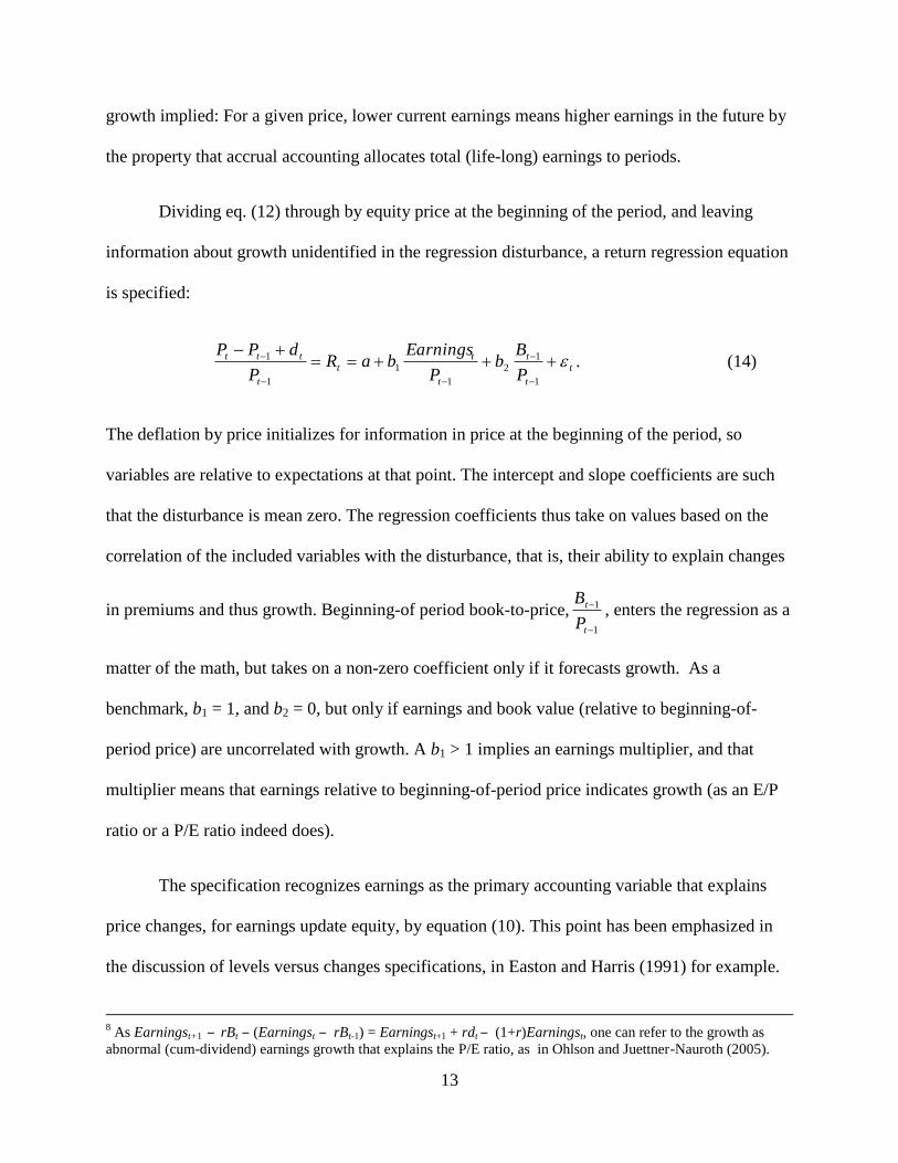
growth implied: For a given price, lower current earnings means higher earnings in the future by

the property that accrual accounting allocates total (life-long) earnings to periods.

Dividing eq. (12) through by equity price at the beginning of the period, and leaving

information about growth unidentified in the regression disturbance, a return regression equation

is specified:

t

t

t

t

t

t

t

ttt

P

Bb

P

EarningsbaR

P

dPP

1

1

2

1

1

1

1 . (14)

The deflation by price initializes for information in price at the beginning of the period, so

variables are relative to expectations at that point. The intercept and slope coefficients are such

that the disturbance is mean zero. The regression coefficients thus take on values based on the

correlation of the included variables with the disturbance, that is, their ability to explain changes

in premiums and thus growth. Beginning-of period book-to-price,1

1

t

t

P

B, enters the regression as a

matter of the math, but takes on a non-zero coefficient only if it forecasts growth. As a

benchmark, b1 = 1, and b2 = 0, but only if earnings and book value (relative to beginning-of-

period price) are uncorrelated with growth. A b1 > 1 implies an earnings multiplier, and that

multiplier means that earnings relative to beginning-of-period price indicates growth (as an E/P

ratio or a P/E ratio indeed does).

The specification recognizes earnings as the primary accounting variable that explains

price changes, for earnings update equity, by equation (10). This point has been emphasized in

the discussion of levels versus changes specifications, in Easton and Harris (1991) for example.

8 As Earningst+1 ‒ rBt ‒ (Earningst ‒ rBt-1) = Earningst+1 + rdt ‒ (1+r)Earningst, one can refer to the growth as

abnormal (cum-dividend) earnings growth that explains the P/E ratio, as in Ohlson and Juettner-Nauroth (2005).

14

Accordingly, the original Ball and Brown (1968) study, with its earnings change variable did not

quite have it right, though the paper certainly stands as a correlation exercise (and reports robust

correlations indeed). The formulation here points to the reason why changes in earnings might

enter the regression: Changes in earnings (growth in earnings) have an informational role if they

forecast subsequent growth that induces a change in premium. The specification also recognizes

a role for book value (other than for the case where Pt = Bt): Book-to-price loads with a non-

zero b2 coefficient if it indicates growth, a point explored later in the paper. The exception is the

case of no change in premium (no growth) where b1 = 1, and b2 = 0.9 Since Ohlson (1995),

researchers have added book value to returns-earnings regressions, but without recognition of

what they are capturing: growth.

One final point that is relevant to material later in this paper: Eq. (12) applies for both

efficient and inefficient market prices; that is, a change in premium may be due to information

about growth but could also be due to the market mispricing earnings and information about

growth.

2.2 An Illustration: the Pricing of Earnings and Cash Flows

In contemporaneous return regressions, capital markets research typically presumes that market

is efficient in pricing information and thus interprets the association of accounting numbers with

returns as indicative of their information content. Here we summarize the Penman and Yehuda

(2009) application of the above framework to the issue of the pricing of earnings and cash flows.

This is an important issue, for accounting is distinguished by its embrace of accrual accounting

(in eq. 6, 7, and 10) as opposed to cash accounting in eq. (3). Numerous studies have run

9 This resonates with the Ohlson (1995) and Feltham and Ohlson (1995) valuation models where price is expressed

as a weighted average of earnings and book value but with the weights shifting completely to book value for Pt = Bt

and completely to earnings for the case where earnings are sufficient.

15

regressions of returns on earnings and cash flows (and various transforms of these measures) and

have found that both are positively related to returns, on average, with both providing

―incremental information content‖ over the other (see, for example, Rayburn 1986; Wilson 1987;

Dechow 1994; Bowen, Burgstahler and Daley 1987; Clubb 1995; Francis, Schipper and Vincent

2003).

Bringing accounting structure to the issue provides a prediction that conflicts with these

findings: Free cash flow decreases net operating assets (NOA) in eq. (6) but also decreases net

debt in eq. (7) so, as Bt = NOAt ‒ Net Debtt, shareholders equity is unaffected by free cash flow.

Indeed , eq. (10) shows that, in the updating of book value, ΔBt, earnings are important but free

cash flow drops out in the calculation; accrual accounting implicitly embraces the tenet of

modern finance that cash flows are irrelevant to shareholder value. In short, the coefficient on

cash flow should be zero. Does the market price the accounting numbers as if earnings add to

price but cash flow does not? The following regression specification (with annual returns)

conforms to eq. (14) but adds free cash flow,

__________________________________________________________________________

t

t

t

t

t

t

t

t

t

t

tt

P

FCFb

P

db

P

Bb

P

Earningsba

P

PP

1

4

1

3

1

1

2

1

1

1

1

Coefficients 0.04 1.69 0.08 -2.88 -0.03

t- statistics 1.37 8.38 4.96 -5.62 -1.12 Average R2

= 0.14

Period: 1963-2001

___________________________________________________________________________

16

Dividends (the cash flow to shareholders) have been moved to the right-hand side as a possible

information variable (in accordance with the literature that sees a ―signaling‖ role for dividends).

The estimates are from Penman and Yehuda (2009) where regressions are run in cross-section

every year from 1963-2001 on NYSE and AMEX firms. Mean coefficient estimates are reported

under the regression equation, along with t-statistics estimated from the time series of regression

coefficients (in the mode of Fama and MacBeth). It is clear that earnings are positively related to

price changes, but the estimated coefficient on free cash flow is not significantly different from

zero, in accordance with the accounting: Given earnings, free cash flow is irrelevant to the

updating of the book value of equity and, given earnings and book value, free cash flow is

irrelevant to the updating of price. Market pricing affirms the accounting. This comes from

attention to specification, and note that the average R2 of 14% is significantly higher than that

typically observed in capital markets research.

The coefficient on earnings is greater than the benchmark of b1 = 1.0, and the framework

supplies the interpretation: Earnings (relative to beginning-of-period price) is correlated with

information about growth and thus takes on a growth multiplier. Note also that b2 is greater than

zero, indicating that book-to-price forecasts growth, a point we will have much to say about

later.10

The zero coefficient on cash flow also has a corresponding interpretation: Given

earnings, book value, and dividends, free cash flow is not an indicator of growth on average.

These regression findings pertain to the pricing of the equity. Corresponding regressions

can be developed for the operations, that is, for the pricing of the firm (the enterprise) rather than

10

The dividend variable takes a negative coefficient, consistent with the dividend displacement property of

dividends reducing prices prices. The size of the coefficient―less than the -1.0 predicted for dividend

displacement―indicates that more dividends (relative to price) indicate lower growth, given earnings and book

values. (Dividend changes added to the regressions load with a positive coefficient, consistent with the dividend

signaling conjecture.)

17

the equity. Assuming that market value of net debt is equal to its book value, the price of the net

operating assets (the price of the firm or enterprise price),tt

NOA

t DebtNetPP . Following the

same logic that got to eq. (12),

)( t

NOA

tt

NOA

t NOAPNOAP

and

)( t

NOA

tt

NOA

t NOAPNOAP .

But, NOAt = OIt – FCFt, by the stocks-and-flows equation for operating activities, eq. (6), so

substituting for ΔNOAt and deflating by the beginning-of-period market value of the operations,

the unlevered version of regression eq. (14) is as below. The operating income yield, NOA

t

t

P

OI

1

(the

enterprise earnings yield) replaces the earnings yield, the enterprise book-to-price replaces equity

book-to-price, and the dividend from operations to all claimants (free cash flow) replaces the

dividend to shareholders.

______________________________________________________________________

tNOA

t

t

NOA

t

t

NOA

t

t

NOA

t

NOA

t

NOA

t

P

FCF

P

NOA

P

OI

P

PP

1

3

1

1

2

1

1

1

1 (15)

Coefficients 0.01 2.21 -0.01 -1.10

t-statistics 0.37 12.63 -0.62 -24.71 Average R2 = 0.22

Period: 1963-2001

_______________________________________________________________________

18

Operating income loads with a multiplier, 2.21, but the coefficient on free cash flow is negative:

Given operating income and book value, higher free cash flow means lower enterprise value.

This accords with the accounting, as stated in the stocks-and-flows equation for operations:

NOAt = OIt – FCFt, that is, operating income adds to the book value for operations but free

cash flow reduces book value, and the market prices firms in the same way on average.

Effectively, free cash flow is a payout from the firm (that reduces its value), with that payout

distributed to the shareholders and net debtholders, as in eq. (1). Note that the average R2 of 22

percent is quite impressive for a returns regression with just three accounting variables.

The earlier research that documented positive coefficients on cash flows dealt with cash

flow from operations (CFO) rather than free cash flows. The following regression maintains this

focus by dividing free cash flow into cash flow from operations and cash investment (I): FCFt =

CFOt ‒ It,. The period covered is 1987 - 2001, with 1987 marking the advent of the modern cash

flow statement in the U.S.

___________________________________________________________________________

tNOA

t

tI

NOA

t

tCFO

NOA

t

t

NOA

t

t

NOA

t

NOA

t

NOA

t

P

I

P

CFO

P

NOA

P

OI

P

PP

1

3

1

3

1

1

2

1

1

1

1 (15a)

Coefficient 0.02 1.68 0.02 -0.98 1.30

t-statistic 0.53 12.42 0.60 -15.53 12.88 Average R2 = 0.15

Period: 1987-2001

___________________________________________________________________________

19

The estimated coefficient on Investment is 1.30, with the market saying that a dollar of

investment is worth $1.30 on average. That is what one expects with positive net-present-value

(NPV) investing. Interpreted within the regression framework, positive-NPV investment adds to

earnings growth and that is growth that the market prices as adding value. The coefficient on

CFO is very close to -1.0: a dollar of cash from operations reduces the price of the firm by a

dollar, on average. This is very different from prior research that reports a positive coefficient on

cash flows, but accords with the accounting. First, cash flows from operations pertain to the firm,

not the equity. Second, in evaluating CFO, one must control for investment of cash back into the

firm. Just like sales must be recognized in evaluating cost of goods sold according to an

accounting relation, so must cash investment in evaluating cash flow from operations: FCFt =

CFOt ‒ It,. The finding also accords with the economics (that the accounting recognizes):

Residual cash (after investing in the business) is invested debt assets, used to reduce debt

obligations, or pay dividends, and these activities are broadly viewed in the theory of finance as

zero-net-present-value activities. Accordingly, the cash flow is valued as reducing the value of

the firm dollar-for dollar, unlike cash investment in the business that adds value to the business

and is valued on average at $1.30 per dollar. The accounting structure captures this, and so does

the market. But note that the market’s pricing of the accounting is only identified with the

appropriate specification.

2.3 Research Directions

These findings have immediate implications. They broadly affirm accrual accounting for

financial reporting (and the dismissal of cash accounting). They report the typical multiplier on

20

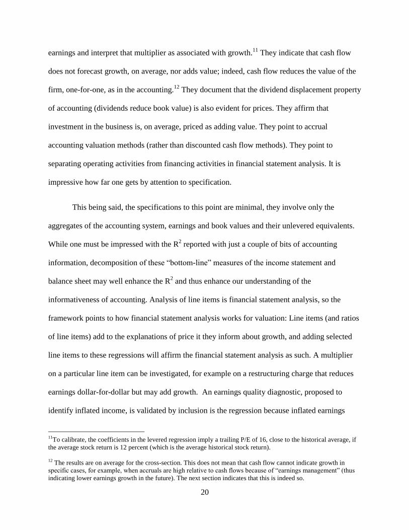
earnings and interpret that multiplier as associated with growth.11

They indicate that cash flow

does not forecast growth, on average, nor adds value; indeed, cash flow reduces the value of the

firm, one-for-one, as in the accounting.12

They document that the dividend displacement property

of accounting (dividends reduce book value) is also evident for prices. They affirm that

investment in the business is, on average, priced as adding value. They point to accrual

accounting valuation methods (rather than discounted cash flow methods). They point to

separating operating activities from financing activities in financial statement analysis. It is

impressive how far one gets by attention to specification.

This being said, the specifications to this point are minimal, they involve only the

aggregates of the accounting system, earnings and book values and their unlevered equivalents.

While one must be impressed with the R2 reported with just a couple of bits of accounting

information, decomposition of these ―bottom-line‖ measures of the income statement and

balance sheet may well enhance the R2 and thus enhance our understanding of the

informativeness of accounting. Analysis of line items is financial statement analysis, so the

framework points to how financial statement analysis works for valuation: Line items (and ratios

of line items) add to the explanations of price it they inform about growth, and adding selected

line items to these regressions will affirm the financial statement analysis as such. A multiplier

on a particular line item can be investigated, for example on a restructuring charge that reduces

earnings dollar-for-dollar but may add growth. An earnings quality diagnostic, proposed to

identify inflated income, is validated by inclusion is the regression because inflated earnings

11

To calibrate, the coefficients in the levered regression imply a trailing P/E of 16, close to the historical average, if

the average stock return is 12 percent (which is the average historical stock return).

12

The results are on average for the cross-section. This does not mean that cash flow cannot indicate growth in

specific cases, for example, when accruals are high relative to cash flows because of ―earnings management‖ (thus

indicating lower earnings growth in the future). The next section indicates that this is indeed so.

21

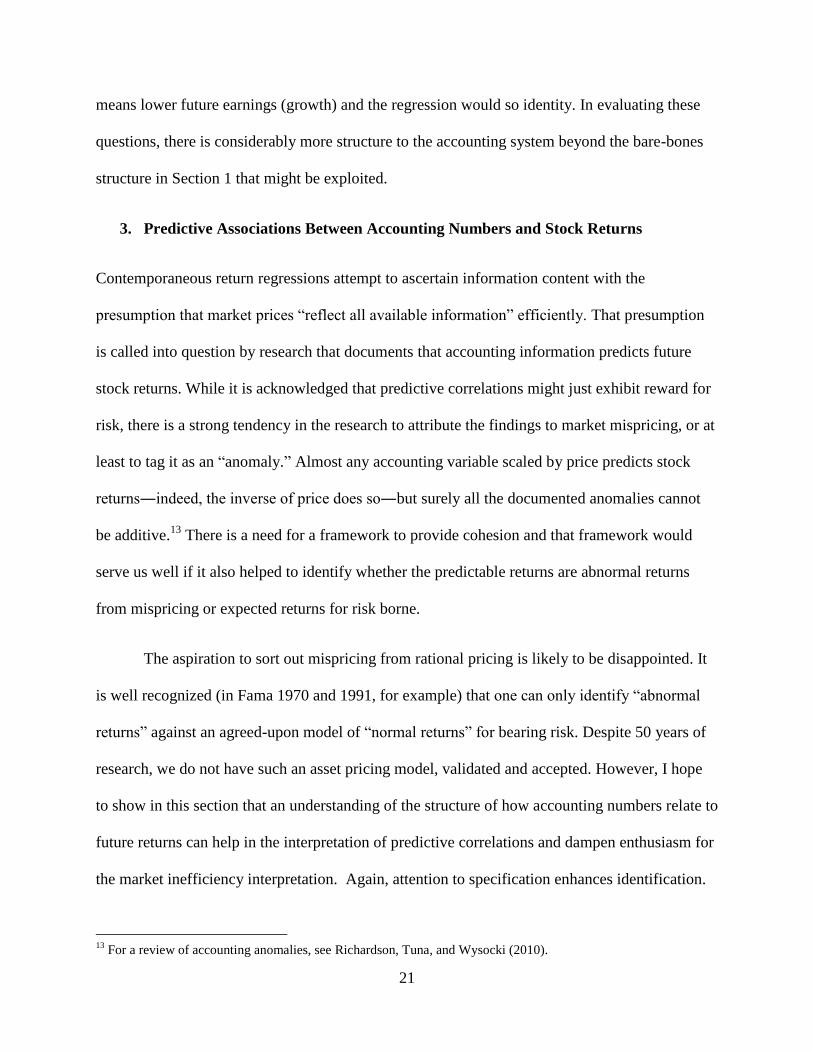
means lower future earnings (growth) and the regression would so identity. In evaluating these

questions, there is considerably more structure to the accounting system beyond the bare-bones

structure in Section 1 that might be exploited.

3. Predictive Associations Between Accounting Numbers and Stock Returns

Contemporaneous return regressions attempt to ascertain information content with the

presumption that market prices ―reflect all available information‖ efficiently. That presumption

is called into question by research that documents that accounting information predicts future

stock returns. While it is acknowledged that predictive correlations might just exhibit reward for

risk, there is a strong tendency in the research to attribute the findings to market mispricing, or at

least to tag it as an ―anomaly.‖ Almost any accounting variable scaled by price predicts stock

returns―indeed, the inverse of price does so―but surely all the documented anomalies cannot

be additive.13

There is a need for a framework to provide cohesion and that framework would

serve us well if it also helped to identify whether the predictable returns are abnormal returns

from mispricing or expected returns for risk borne.

The aspiration to sort out mispricing from rational pricing is likely to be disappointed. It

is well recognized (in Fama 1970 and 1991, for example) that one can only identify ―abnormal

returns‖ against an agreed-upon model of ―normal returns‖ for bearing risk. Despite 50 years of

research, we do not have such an asset pricing model, validated and accepted. However, I hope

to show in this section that an understanding of the structure of how accounting numbers relate to

future returns can help in the interpretation of predictive correlations and dampen enthusiasm for

the market inefficiency interpretation. Again, attention to specification enhances identification.

13

For a review of accounting anomalies, see Richardson, Tuna, and Wysocki (2010).

22

The relationship between accounting numbers and future returns is identified via the

same structure that led to eq. (12) and (14) for contemporaneous returns, but now with expected

t+1 returns identified with expectations of t+1 earnings and the expected t+1 change in

premium. Rolling eq. (12) forward one period and deflating by the current price,

t

tttt

t

t

t

t

ttt

P

BPBPE

P

EarningsERE

P

dPPE )()()()(

)( 111

1

1

. (16)

The deflation by Pt yields the expected t+1 rate-of-return on the left hand side. It also deflates

the right-hand side for the market’s expectation, at time t, of forward (t+1) earnings and the

change in premium and for the risk surrounding those expectations (that discounts the price).

Moving to the resulting regression specification, as before,

t

t

t

t

t

tP

Bb

P

EarningsEbaR

2

1

11

)(. (17)

Eq.(17) identifies the expected year-head return via the forward earnings yield and the current

book-to-price. If b1 = 1.0 and b2 = 0, the expected t+1 return is given by the forward earnings

yield and the analysis in the last section shows that this is the case where price equals book value

or where the is no expected change in the premium, that is, no expected growth. Valuation theory

so affirms: the E/P ratio equals the required return with no growth. But there is a further insight:

Any variable that forecasts a change in premium (discounted for the market’s risk-adjusted

expectation at time t) will also forecast expected returns. As explained in the last section, that is a

forecast of growth, so any variable that forecasts growth that is priced as risky will add to the

explanation of expected returns.

23

The identification of book-to-price (B/P) in eq. (17) sets off bells because the Fama and

French asset pricing model identifies book-to-price as indicating firms’ sensitivity to factors that

are priced as risky. The identification of the expected return via E/P, B/P, and growth is taken up

in the next section. Here we apply the framework to the interpretation of predictive return

correlations in accounting research. In regression format, that research typically has t+1 returns

on the left-hand side, as in eq. (17), and accounting variables like accruals and growth in net

operating assets (ΔNOA) on the right-hand side. More often, tests compare future returns on

portfolios formed on the accounting variable, thus replicating feasible trading strategies (and

avoiding the linear constraint of (linear) regressions). Controls are introduced for ―risk factors,‖

with the predictable return that is left unexplained by these risk factors then identified as an

―anomaly‖ or, more boldly, as ―abnormal returns‖ to mispricing. But there is the difficulty: We

do not have an acceptable asset pricing model to establish ―normal returns‖ for risk. Indeed,

adding variables like B/P, size, and ―momentum‖ as controls for risk is mere conjecture, for

these variables have been included in nominated asset pricing merely by observing

correlations—data dredging—not from analytical development. In short, there has been little

attention to specification, neither in anomaly research nor in the identification of benchmarks

against which an anomaly is imputed. This leaves an interpretive mess; the attribution to

―abnormal returns‖ is a stab in the dark.

Eq. (16) and (17) help sort things out. Suppose one documents that earnings-to-price

predicts returns, as in Basu (1977) and (1983) and were tempted to designate the correlation as

an ―anomaly‖ (as in the Basu papers). That would be overreaching as an inference, for the

structure that connects accounting numbers to expected returns says that (forward) earning-to-

price should predict returns under rational pricing: The earnings yield is an indication of risk and

24

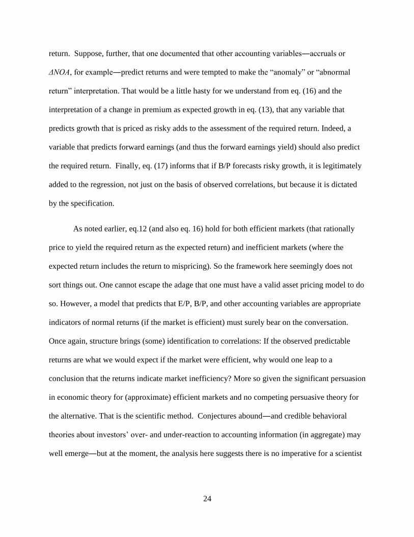
return. Suppose, further, that one documented that other accounting variables―accruals or

ΔNOA, for example―predict returns and were tempted to make the ―anomaly‖ or ―abnormal

return‖ interpretation. That would be a little hasty for we understand from eq. (16) and the

interpretation of a change in premium as expected growth in eq. (13), that any variable that

predicts growth that is priced as risky adds to the assessment of the required return. Indeed, a

variable that predicts forward earnings (and thus the forward earnings yield) should also predict

the required return. Finally, eq. (17) informs that if B/P forecasts risky growth, it is legitimately

added to the regression, not just on the basis of observed correlations, but because it is dictated

by the specification.

As noted earlier, eq.12 (and also eq. 16) hold for both efficient markets (that rationally

price to yield the required return as the expected return) and inefficient markets (where the

expected return includes the return to mispricing). So the framework here seemingly does not

sort things out. One cannot escape the adage that one must have a valid asset pricing model to do

so. However, a model that predicts that E/P, B/P, and other accounting variables are appropriate

indicators of normal returns (if the market is efficient) must surely bear on the conversation.

Once again, structure brings (some) identification to correlations: If the observed predictable

returns are what we would expect if the market were efficient, why would one leap to a

conclusion that the returns indicate market inefficiency? More so given the significant persuasion

in economic theory for (approximate) efficient markets and no competing persuasive theory for

the alternative. That is the scientific method. Conjectures abound―and credible behavioral

theories about investors’ over- and under-reaction to accounting information (in aggregate) may

well emerge―but at the moment, the analysis here suggests there is no imperative for a scientist

25

to ascribe returns to accounting numbers as anomalies if those numbers forecast forward

earnings or growth.

To appreciate the point, consider the predictable returns associated with E/P documented

by Basu 1977 and 1983 and many others with the attribution of ―anomalous returns.‖ Ball (1978)

made the straight-forward conjecture that earnings-to-price is a yield (a return on price) which,

like a bond yield, might be related to risk. But that conjecture becomes an imperative only with a

formal model of how the earnings yield relates to risk and return. A bond model supplies it: the

expected yield is identified via an internal rate-of-return calculation. (Accounting-wise, the

effective interest method calculates the expected earnings yield.) The yield on a bond is readily

accepted as an indication of its risk and required return even though we do not have ―a generally

accepted equilibrium asset pricing model‖ for a bond (or any asset). Accordingly, it would be

considered quite brazen to claim that predictable bond returns from bond yields are anomalous.

For the equity earnings yield the issue is more difficult, for two reasons. First, unlike a

bond yield, the earnings yield also reflects anticipated earnings growth, so an internal rate-of-

return calculation from an equity valuation model must accommodate a growth forecast, but

forecasts of (long-term) growth are elusive. Indeed, growth may be related to risk.14

Second,

earnings is an accounting measure―it depends of how the accounting is done―and there is no

guarantee that the GAAP earnings yield captures risk and return. But our framework

accommodates both earnings measurement and growth (they are in fact complements) and, with

the discount for risk in Pt in eq. (16), admits only those variables that predict risk-adjusted

growth. Indeed, the model for the expected return here is a generalization of the bond return

14

Papers that have tried to estimate the ―implied cost of capital‖ for equity as an internal rated of return from growth

forecasts have been remarkably unsuccessful in producing measures that validate against subsequent average

returns. See Easton (2009) for a review.

26

model where there is no growth (and no expected change in premium) for equities where there is

likely to be growth.15

The empirical question, then, is whether so-called anomaly variables predict returns

because they predict the forward earnings yield and the change in premium (growth) in eq. (16).

If so, they would be part of a rational determination of the required return for risk. A literature

survey reveals that prominent accounting anomalies are accruals (in Sloan 1996), growth in net

operating assets, ΔNOA (in Fairfield, Whisenant, and Yohn 2003), and return on assets (Chen,

Novy-Marx, and Zhang 2010). These are primary candidates for explaining expected returns in

this framework for they are likely to forecast forward earnings and possibly growth.16

As

Earningst = CFOt + Accrualst (in the way that accruals are defined in accrual anomaly papers),

specifying accruals effectively decomposes Earningst into cash flow and accrual components,

and these two components have different implications for forecasts of forward earnings in Sloan

1996. It is the market’s failure to recognize the difference in ―persistence‖ of cash flows and

accruals that is said to be the reason for the accrual anomaly, but a rational market recognizes

such a difference―and the reversal property of accruals―in forecasting forward earnings and

the expected return in eq. (16). With respect to ΔNOA, Earningst + Net Interestt (after-tax) =

Operating incomet (after-tax) = Free cash flowt – ΔNOAt by the clean surplus equation for

operating activities (6), so ΔNOAt also decomposes the operating component of earnings into

components that may have different implications for forward earnings. The framework also

15

Model (11) is the return model for a bond. With mark-to-market accounting, the premium is zero (and thus the

change in premium is zero).

16

There are many reported accounting ―anomalies‖ but many are related to the three here. The ―growth in total

assets anomaly‖ is related to growth in net operating assets, as is growth in long-term NOA (in Fairfield, Whisenant,

and Yohn 2003). Anomalous returns are also associated with investment (in Chen, Novy-Marx, and Zhang 2010 ),

but investment is part of ΔNOAt = It + Other Operating Accrualst (eq. (6a).

27

suggests it is no surprise that return on assets predicts returns for is contains both earnings and

the book value that are involved in the return on assets calculation.

Moreover, considerable empirical work indicates that return on assets is a robust

predictor of future earnings. Indeed Penman and Zhang (2006) find that return on assets (or

rather return on net operating assets) and ΔNOA are the primary forecast variables and explain

why this would be so as a matter of accounting structure. As ΔNOAt = It + Other Operating

Accrualst (eq. 6a), accruals (and indeed investment in Chen, Novy-Marx, and Zhang 2010) adds

to the forecast of forward earnings. The relationship between these variables and future growth is

less clear, but ΔNOA is a growth variable.

Penman and Zhu (2010, in progress) indicate that accruals, ΔNOA, and return on assets

indeed forecast forward earnings and growth (among a number of other anomaly variables they

look at). The panels below provide a summary. Again the regressions are run in the cross-section

in Fama and Macbeth style over the period, 1962 to 2009. Regression (18) estimates the

association between of forward earnings-to-price with and a number of time-t variables. The

starting point is current earnings-to-price, to which is added the B/P ratio, as in the return model

(17), current changes in earnings (over price), and then the anomaly variables, At, one at a time.17

17

The three anomaly variables are measured as in the papers referenced above. Pt is observed four months after

fiscal-year end (by which time accounting data for the prior fiscal year, dated t, will have been reported). Earnings

are before extraordinary and special items, with a tax allocation to special items. Results are similar when accruals

and ΔNOA are price deflated. The top and bottom 1% of each predictor variable is rejected each year in estimating

the regressions.

28

__________________________________________________________________________

Forecasting the Forward Earnings Yield

14321

1

tt

t

t

t

t

t

t

t

t AP

Earnings

P

B

P

Earnings

P

Earnings (18)

No anomaly variables

Coefficient 0.028 0.450 -0.005 -0.110

t-statistic 6.84 16.70 -0.94 -2.14 Average R2 = 0.29

At = Accruals/Average Assets

Coefficient 0.027 0.473 -0.006 -0.112 -0.050

t-statistic 6.84 18.32 -1.22 -2.33 -4.08 Average R2 = 0.30

At = ΔNOA/Average Assets

Coefficient 0.033 0.479 -0.007 -0.126 -0.052

t-statistics 7.23 18.32 -1.42 -2.15 -5.26 Average R2 = 0.30

At = Return on Assets

Coefficient 0.021 0.610 -0.009 -0.106 0.028

t-statistic 5.83 20.61 -1.77 -2.18 1.84 Average R2 = 0.26

_______________________________________________________________________

These results confirm that trailing E/P is positively correlated with forward E/P, so the

findings of Basu (1977 and 1983) are identified with rational pricing. Given current earnings-to-

price, book-to-price appears to have little role in forecasting the forward earnings yield, but the

anomaly variables do. Significantly, they do so in the direction in which they forecast returns:

Higher accruals and ΔNOA forecast lower forward earnings than current earnings, just as they

forecast lower returns, and return of assets forecasts higher forward earnings, as it does returns.

The coefficient on return on assets is not large, but the regression already includes earnings and

29

book value which are the leveraged equivalents of the numerator and denominator of return on

assets.

Models for forecasting growth are in the next panel. The forecast variable is the earnings

growth rate two years ahead, that is, the growth after year t+1 that is forecasted in predicting the

t+1 change in premium in eq. (16) and thus the expected return. Two-year-ahead growth is of

course only a small part of long-term growth so clearly this is a feeble attempt to develop a

forecast (and the R2 are also feeble). Again, the forecasts retain E/P and B/P, as in eq. (17). The

current change in earnings is added in the first model, but it is not significant so is dropped in the

models that add the anomaly variables.18

18

The earnings change, both in t+2 and t, are after reinvesting dividends at the risk-free rate to adjust for the

displacement property of dividends (and thus the notation, Earningsa). To handle negative earnings, the t+2

earnings growth rate is calculated as

12

2 2

t

a

t

a

t

EarningsEarnings

Earningswhich ranges from -2.0 to 2.0. Only firms that survive two years ahead are included in

the estimations.

30

____________________________________________________________________________

Forecasting Earnings Growth

24321

1

2

tt

t

a

t

t

t

t

t

t

a

t uAP

Earnings

P

B

P

Earnings

Earnings

Earnings

(19)

No anomaly variables

Coefficient -0.034 -0.926 0.098 -0.163

t-statistic -1.50 -7.08 5.62 -1.33 Average R2 = 0.02

At = Accruals/Average Assets

Coefficient -0.032 -1.002 0.092 -0.264

t-statistics -1.39 -6.31 5.31 -4.19 Average R2 = 0.02

At = ΔNOA/Average Assets

Coefficient -0.015 0.987 0.089 -0.135

t-statistic -0.69 -6.89 5.16 -4.54 Average R2 = 0.02

At = Return on Assets

Coefficient 0.025 0.775 0.073 -0.799

t-statistic 0.75 -4.52 3.69 -5.28 Average R2 = 0.03

The current E/P loads with a strong negative coefficient as expected, for E/P (or rather

P/E) indicates growth. The strong positive coefficient on B/P is the focus of the next section of

the paper, but note that B/P forecasts growth. The sign of the estimated coefficients on accruals

and ΔNOA imply lower expected growth, and that is consistent with their relationship with future

returns: If growth is priced as risky, higher accruals and ΔNOA that imply lower growth also

imply lower expected returns that reflect that risk.

31

In conclusion, both the forward earnings regressions and the growth regressions suggest

that the so-called anomalies are consistent with the rational pricing of risk. An alternative

interpretation requires something else to be put on the table. A behavioral theory, duly validated,

might supply this (though not a behavioral conjecture), but that would have to challenge the

economic theory of rational pricing with which the findings reported here, from Penman and Zhu

(2010, in progress), are consistent. Researchers claim that the returns to anomalies that they

document—in many cases 10 percent or more per year on average—are too large to be explained

as return for risk. But surely that much money cannot be left on the table and so easily detected

ex ante (10 percent per year!)? There is another explanation: Growth is risky and the last half of

the twentieth century when these returns were observed were years when growth paid of

handsomely, ex post. In contrast, positions based on the anomalies apparently performed badly in

2008-2009 when growth expectations took a big shock.

3.3 Further Research

Forecasting and pricing go together, for price is based on expected future payoffs. The question

thus arises as to how forecasting models are to be structured. Models (18) and (19) presumably

can be improved upon and, once again, accounting structure implies a structure for a forecasting

model. First, eq. (10) says that a forecast of earnings must be consistent with a forecast of change

in equity and dividends, and eq. (6) says that forecasts of operating income must reconcile to

forecasts of free cash flow and growth in net operating assets. A purely statistical approach can

produce forecasts outside of these bounds; the accounting structure implies constraints on (the

coefficients of) forecasting models. Second, not only must line items (that may appear in a

forecasting model) tie to each other in a structured way according to accounting relations, but the

inter-temporal properties of accounting should also be recognized in constraining the forecasts;

32

current earnings and accruals have implications for future earnings and accruals, for example, as

a feature of accounting measurement. At a practical level, a accounting structure supplies the

architecture for a forecasting spreadsheet: one forecasts a set of future financial statements that

maintain the accounting relations Penman and Zhang (2006), Penman (2010), and Penman

(2011, Chapter 6) elaborate. See also Christodoulou and McLeay (2010).

Most research on forecasting has focused on forecasting future earnings as payoffs. But

this section points to another aspect of forecasting: estimating the required return that discounts

those forecasted payoffs. The forecasting variables would be identified via forecasts of the

forward earnings yield and growth, validated by their ability to predict stock returns. This would

be a ―third way‖ in estimating the cost of capital over both the standard asset pricing models of

finance and the approach in accounting of inferring the ―implied cost of capital‖ as an internal

rate-of-return calculation that reconciles forecasts of earnings and growth to the current price.

The problem with both approaches is that the inputs are expectations, of risk premiums and

covariances in asset pricing models and forward (analyst) earnings estimates and long-term

growth rates in the accounting approach. In the latter case, the specification of a growth rate

(often specified as a constant for all firms) is particularly problematical, as is the use of analysts’

expectations, and the resulting estimates of the cost-of-capital do not appear to be validated on

the basis of subsequent realized returns. The ―third way‖ would input current observables not

expectations, as above, with the implications for growth identified in the estimation of the return

regression equation and with a validation with forecasting regressions like those above. The

identified variables would presumably include (a parsimonious set of) the so-called anomaly

variables. Whether this would all work out is a question of appropriate specification but

33

ultimately an empirical issue. But note how easy it is to show that ―anomaly‖ variables predict

returns whereas estimates of the implied cost-of-capital typically fail to do so.

The ―third way‖ assumes market efficiency if one has the cost-of-capital in mind, but so

do the other two approaches. Again, in the absence of an agreed-upon asset pricing model, we

can only estimate the expected return to buying at the current market price. It is the issue of asset

pricing models to which we now turn.

4. Predictive Correlations, Risk, and Asset Pricing

The appearance of book-to-price (B/P) in the prediction of future returns in regression equation

(17) is noteworthy because B/P features prominently in the three-factor asset pricing model of

Fama and French (1993 and 1996) and in four-factor models that add momentum and other

factors. Asset pricing researchers are largely mystified as to why book-to-price would be a risk

factor, grasping at conjectures that include ―distress factor,‖ ―the risk of assets in place,‖ and

―growth options.‖ These asset pricing models have been proposed simply on the basis of

correlations observed in the data; B/P takes prominence because it appears to be a primary

predictor of stock returns historically. Again, correlations without specification cannot get us far

in our understanding. The Capital Asset Pricing Model was developed analytically, but not these

models; they come from data dredging (factor dredging, as it is called). One cannot have

confidence in a model that is purely a fit to the data.

The analytical development of an asset pricing model that identifies relevant factors is a

tall order. The empirical approach to the identification involves estimating (what the asset

pricing literature calls) characteristic regressions―cross-sectional regressions of future returns

on firm characteristics. Characteristics that are found to be significant in these regressions―like

34

beta, firm size, and B/P―become the feature for forming ―factor mimicking‖ portfolios whose

returns are said to represent outcomes to risk that cannot be diversified away. ―Factor

regressions‖ then estimate firms’ sensitivity to these common factors. The observation that

returns of firms with a common attribute covary together and with returns on portfolios formed

on the attribute is seen as a validation of sensitivity to common (non-diversifiable) risk. But this

is, again, a fit to data; as Daniel and Titman (1997) point out, returns can covary with common

characteristics rather than a common risk factor.

While the derivation of an asset pricing model is elusive, one might at least require the

characteristic regressions to be well specified, but those that have been estimated just report

correlations discovered from data dredging. The analysis leading to eq. (16) and the regression

eq. (17) supplies some understanding.19

First and foremost, in relating accounting numbers to future returns, forward E/P is the

starting point, not B/P. Indeed B/P is not relevant in the no-growth case. The identification of the

forward earnings yield makes sense: investors buy earnings and earnings are at risk. Indeed,

much accounting research, from Ball and Brown (1968) and Beaver (1968) onwards, shows that

realized stock returns, the outcome to risk, are driven by earnings realizations that differ from

expectation. Yet E/P is missing from the Fama and French model (although note that E/P and

B/P are positively correlated).

Second, B/P enters in regression (17) if (and only if) it predicts growth and that growth is

priced as risky. So B/P is identified as an appropriate characteristic on which to build an asset

19

The four-factor model of Chen, Novy-Marx, and Zhang (2010 ) has a return-on-assets factor and an investment

factor but these are also variables identified in the last section as forecasting the forward earnings yield and growth

(investment is part of ΔNOA).

35

pricing model, with a rationale supplied; B/P in an asset pricing model is no longer a mystery

subject to conjecture.

One might query whether B/P forecasts growth because the standard notion is that P/B,

not B/P, indicates growth. But one understands from eq. (12) and (16) that B/P cannot be

considered without E/P, and E/P imbeds a growth forecast; B/P (not P/B) has a role in

forecasting growth for a given E/P. The association between B/P and future earnings growth in

regression (19) indicates that B/P indeed forecasts growth in addition to E/P. This is also

documented in Penman and Reggiani (2010), as the panel below demonstrates. For this

presentation, firms are ranked each year, 1963-2006, on their estimated forward P/E and then,

within each P/E portfolio, on their B/P. The numbers are average earnings growth rates two years

ahead. Mean growth rates are positively associated with P/E, as one would expect, but for a

given P/E are also positively associated with B/P.

Mean Percentage Earnings Growth Rates Two Years Ahead for Portfolios formed on P/E

and B/P; 1963-2006

Low 2 3 4 High

High-

Low

Ranking on P/E -5.5 -0.4 0.0 4.2 26.1 31.6

R

an

kin

g o

n B

/P

Low -11.5 -5.9 -4.6 -4.8 15.2

2 -5.6 -1.6 -3.2 -1.6 19.6

3 -5.9 -0.1 -3.6 3.3 25.8

4 -3.1 0.6 0.6 5.8 30.1

High -2.0 3.6 10.7 18.7 38.0

High-

Low 9.5 9.5 15.3 23.5 22.8

36

The observation that B/P forecasts growth may have nothing to do with risk and return,

but Penman and Reggiani (2010) indicate that the expected growth forecasted by B/P is indeed

risky. The panel below reports the standard deviation of growth rates for each portfolio over the

years. The standard deviations are clearly related to the mean growth rates (and to B/P). A

similar pattern is observed for the inter-decile range: For a given E/P, higher B/P is associated

with higher growth rates, on average, but it is growth that is subject to larger shocks. One might

ask if such variation in growth rates is priced as risky—it could be diversifiable risk—but B/P is

denominated in price that discounts for (priced) risk.

Std Dev of Percentage Earnings Growth Rates Two Year Ahead for Portfolios formed on P/E and

B/P ; 1963-2006

Low 2 3 4 High

High-

Low

Ranking on P/E 12.0 9.5 10.7 17.3 19.7 7.7

Ran

kin

g o

n B

/P

Low 15.2 13.2 10.4 16.1 18.9

2 13.3 11.3 11.3 18.5 19.7

3 14.7 11.4 12.0 19.4 21.0

4 14.3 10.2 13.3 21.7 26.2

High 19.3 17.5 19.8 25.7 28.1

High-

Low 4.1 4.3 9.3 9.5 9.2

Are these risky growth expectations actually priced as risky? Here are the year-ahead,

buy-and-hold returns for the 25 portfolios:

37

Mean Percentage Annual Returns for Portfolios formed on P/E and B/P; 1963-2006

Low 2 3 4 High H-L t-stat

Ranking on P/E 23.2 18.1 14.9 12.1 13.5 -9.7 -2.47

Ran

kin

g o

n B

/P

Low 19.7 17.1 14.2 10.9 4.3

2 22.1 16.0 13.0 9.1 8.8

3 21.6 17.0 12.1 8.5 14.4

4 24.3 18.0 14.7 13.4 15.5

High 30.0 22.6 20.2 20.1 26.4

H-L 10.3 5.5 6.1 9.2 22.2

t-stat 3.92 2.92 2.78 2.62 5.67

Clearly, average returns are related to E/P as eq. (16) indicates and, for a given E/P, are related to

B/P as in eq. (17). And the reason is supplied: B/P forecasts growth (that induces an expected

change in premium) and that growth is priced as risky.

Of course, one cannot dismiss the conjecture that these return results are due to market

mispricing. But there are good reasons to suggest that expected growth is priced as risky. Growth

is expected earnings beyond the forward year and, just as forward earnings is priced as risky in

the forward E/P ratio, so would subsequent earnings. Indeed, one expects more earnings (growth)

to come with more risk: A firm typically cannot get more earnings growth without more risk. We

understand, for example, that added leverage adds to expected earnings growth but also adds to

risk, and that risk-return tradeoff, so basic to financial economics, is to be expected of operations

38

also.20

But there is another reason that Penman and Reggiani (2010) highlight, and that has to do

with accounting: Under standard revenue and earnings realization principles, accounting defers

the recognition of earnings until uncertainty is resolved, and deferred earnings is earnings

growth. That is, accommodation for risk is built into the accounting and that risk seems to be

priced by the market. As deferred earnings means lower forward earnings relative to book value,

higher B/P for a given E/P forecasts earnings growth and (if the growth is priced as risky) higher

expected returns. To the theme of this paper, accounting measurement and structure combine to

yield the specification and a prediction as to why E/P and B/P would jointly predict stock

returns: Forward earnings are at risk but so is subsequent expected earnings growth and B/P

pertains to the latter. The E/P and B/P trading strategy has been trolled many times by investors,

but the strategy might be picking up risk.

4.1 Book-to-Price, Leverage, and Returns

A remarkable empirical observation (or lack of it) challenges asset pricing research: While

finance theory predicts that leverage adds to expected return, no one has been able to show

robustly that leverage is rewarded by higher returns in the stock market. Indeed, the correlation is

often negative. Penman, Richardson, and Tuna (2008), for example, document a negative

correlation with forward returns after controlling for B/P and other characteristics in the Fama

and French model.

20

It is always the case that NFE

t

OI

tt

OI

t

E

t ggELEVgg 1 where E

tg is the growth rate for (bottom-line)

earnings, OI

tg is the growth rate in operating income, NFE

tg is the growth rate in net financial expense, and

111 / ttt EarningsNFEELEV measures leverage in the income statement. So, provided leverage is

favorable such that NFE

t

OI

t gg > 0, leverage levers up the growth in earnings.

39

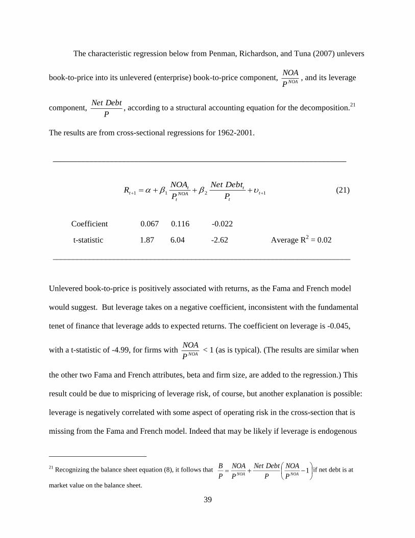
The characteristic regression below from Penman, Richardson, and Tuna (2007) unlevers

book-to-price into its unlevered (enterprise) book-to-price component, NOAP

NOA, and its leverage

component, P

DebtNet, according to a structural accounting equation for the decomposition.

21

The results are from cross-sectional regressions for 1962-2001.

________________________________________________________________________

1211 t

t

t

NOA

t

tt

P

DebtNet

P

NOAR (21)

Coefficient 0.067 0.116 -0.022

t-statistic 1.87 6.04 -2.62 Average R2 = 0.02

_________________________________________________________________________

Unlevered book-to-price is positively associated with returns, as the Fama and French model

would suggest. But leverage takes on a negative coefficient, inconsistent with the fundamental

tenet of finance that leverage adds to expected returns. The coefficient on leverage is -0.045,

with a t-statistic of -4.99, for firms with NOAP

NOA < 1 (as is typical). (The results are similar when

the other two Fama and French attributes, beta and firm size, are added to the regression.) This

result could be due to mispricing of leverage risk, of course, but another explanation is possible:

leverage is negatively correlated with some aspect of operating risk in the cross-section that is

missing from the Fama and French model. Indeed that may be likely if leverage is endogenous

21 Recognizing the balance sheet equation (8), it follows that

1

NOANOA P

NOA

P

DebtNet

P

NOA

P

Bif net debt is at

market value on the balance sheet.

40

such that firms choose lower leverage if they have high operating risk. Our specification of the

appropriate characteristic regression that includes B/P suggests that there is indeed a missing

factor in the Fama and French model: the earnings yield indicates risk and return.

There is a further issue, however, and that is a methodological one. Forward return

regressions like model (21) have notoriously low R2. Misspecification may be the reason, but the

signal-to-noise ratio must also be very low: The variation in realized returns in the cross-section

due to unexpected returns is high relative to the variation in expected returns (see Elton 1999).

The solution to investigating the leverage issue is to move from forward return regressions to

contemporaneous return regressions, but honoring the specification requirements in Section 2.

That is, with an understanding that realized earnings drive realized returns, control for

unexpected returns due to earnings realizations to isolate the effect of leverage.

The results from a regression of this form are below. (Results are from preliminary

research in Penman, Reggiani, Richardson, and Tuna 2010, in progress). Realized levered returns

are unlevered returns (as in model 15) enhanced by leverage, with realized unlevered (enterprise)

E/P, NOA

t

t

P

OI

1

, and the unlevered (enterprise) price book-to-price,NOA

t

t

P

NOA

1

1

, explaining the unlevered

component of returns (as in model 15).22

Both the unlevered E/P and unlevered B/P load with

significant coefficients and, with the control for these two factors, leverage now adds to the

levered return (positively). The coefficient on leverage is not large but the effect of leverage on

realized returns depends on whether the leverage is favorable. For the cases where the unlevered

22 Unlevered returns (for the firm) are

NOA

t

NOA

tt

NOA

t

P

PFCFP

1

1

, with free cash flow in model (15) taking to the left-

hand side as the dividend from the firm to claimants, as in eq. (1).

41

return the realized unlevered return is greater than the risk-free rate, the estimate coefficient on

leverage is 0.40 with a t-statistic of 4.69.

______________________________________________________________________________

1

1

13

1

12

1

1

t

t

t

NOA

t

t

NOA

t

tt

P

DebtNet

P

NOA

P

OIR (22)

Coefficient -0.038 1.830 0.081 0.016

t-statistic -1.23 8.65 3.64 1.45 Average R2 = 0.14

______________________________________________________________________________

In short, attention to specification solves the riddle as to why researchers have not been able to

document positive returns to leverage.

4.2 Further Research

The identified characteristic regressions raise the specter of developing an accounting-based

asset pricing model with common factors identified with the forward earnings yield and expected

growth. A separation of operating activities and financing activities, as in regression (22), would

identify risk associated with operations from the added risk associated with leverage. Observable

attributes that forecast the forward operating income yield and subsequent growth (including the

enterprise book-to-price) would be the basis for constructing factor mimicking portfolios and

firms sensitivities to the returns of those portfolios. The agenda raises hopes of reconciling asset

pricing research with accounting-based valuation to place accounting and finance on the same

platform. Who knows: perhaps an accounting-based asset pricing model will provide a handle to

address the issue of whether accounting anomalies are indeed anomalies?

42

References

Aboody, D., M. Barth, and R. Kasznik. 2004. SFAS No. 123 stock-based compensation

expense and equity market values. The Accounting Review 79 (April), 251-275.

Ball, R., and P. Brown. 1968. An empirical evaluation of accounting income numbers.

Journal of Accounting Research, 6 (Autumn), 159-177.

Ball, R. 1978. Anomalies in relationships between securities’ yields and yield-surrogates.

Journal of Financial Economics 6, 103-126.

Basu, S. 1977. Investment performance of common stocks in relation to their price-earnings

ratios: A test of the efficient market hypothesis. The Journal of Finance 32, 663-682.

Basu, S. 1983. The relationship between earnings yield, market value, and return for NYSE

stocks: further evidence. Journal of Financial Economics 12, 129-156.

Barth, M. 1994. Fair value accounting: Evidence from investment securities and the market

valuation of banks. The Accounting Review 69 (January), 1–25.

Barth, M., W. Beaver, J. Hand, and W. Landsman. 1999. Accruals, cash flows, and equity

values. Review of Accounting Studies 3 (December), 205-229.

Beaver, W. 1968. The information content of annual earnings announcements. Journal of

Accounting Research 6 (Supplement), 67-92.

Bowen, R., D. Burgstahler, and L. Daley. 1987. The incremental information content of accrual

versus cash flows. The Accounting Review 62 (October), 723-747.

Chen, L., R. Novy-Marx, and L. Zhang. 2010. An alternative three-factor model. Unpublished

paper, Washington University in St. Louis, University of Chicago, and University of Michigan.

Christodoulou, D., and S. McLeay. 2010. The double entry constraint and the estimation of the

equilibrium level of accruals. Working paper, Methodological and Empirical Advances in

Financial Analysis (MEAFA), University of Sydney.

Clubb, C. 1995. An empirical study of the information content of accounting earnings, funds

flows and cash flows in the UK. Journal of Business Finance and Accounting 22 (January), 35-

52.

Daniel, K., and S. Titman. 1997. Evidence on the characteristics of cross sectional variation in

stock returns. Journal of Finance 52, 1-33.

Dechow, P. 1994. Accounting earnings and cash flows as measures of firm performance: The

role of accounting accruals. Journal of Accounting and Economics 18 (July), 3-42.

43

Easton, P., and T. Harris. (1991). Earnings as an explanatory variable for returns. Journal of

Accounting Research, 29 (Spring), 9-36.

Easton, P, T. Harris, and J. Ohlson. 1992. Aggregate accounting earnings can explain most of

security returns: The case of long event windows. Journal of Accounting and Economics 15

(June-September), 119-142.

Elton, E. 1999. Expected return, realized return, and asset pricing tests. Journal of Finance 54

(August 1999), 1199-1220.

Fama, E. 1970. Efficient capital markets: A review of theory and empirical work. Journal of

Finance, 25, 383-417.

Fama, E. 1991. Efficient capital markets: II. Journal of Finance 45, 1575-1617.

Fama, E., and K. French. 1993. Common risk factors in the returns of stocks and bonds. Journal

of Financial Economics 33, 3-56.

Fama, E., and K. French. 1996. Multifactor explanations of asset pricing anomalies. Journal of

Finance 51, 55-84.

Feltham, G., and J. Ohlson. 1995. Valuation and clean surplus accounting for operating and

financial activities. Contemporary Accounting Research, 12 (Spring), 689-731.

Fairfield, P., J. Whisenant, and T. Yohn. 2003. Accrued Earnings and Growth: Implications for

Future Profitability and Market Mispricing. The Accounting Review 78 (1): 353-371.

Francis, J., K. Schipper, and L. Vincent. 2003. The relative incremental explanatory power of

earnings and alternative (to earnings) performance measures for returns. Contemporary

Accounting Research 20 (Spring), 121-164.

Landsman, W. 1986. An empirical investigation of pension fund property rights. The Accounting

Review 61 (October), 662-691.

Lipe, R. 1986. The information contained in components of earnings. Journal of Accounting

Research 24 (Supplement), 37-64.

Miller, M., and F. Modigliani. 1961. Dividend policy, growth, and the valuation of shares.

Journal of Business 34, 411-433.

Nurnberg, H. 2006. Perspectives on the cash flow statement under FASB Statement No. 95

Occasional Paper Series, Center for Excellence in Accounting and Security Analysis, Columbia

Business School, at

https://www4.gsb.columbia.edu/null?exclusive=filemgr.download&file_id=104.

44

Ohlson, J. (1995). Earnings, book values, and dividends in equity valuation. Contemporary

Accounting Research, 12 (Spring), 661-687.

Ohlson, J., and B. Juettner-Nauroth. 2005. Expected EPS and EPS growth as determinants of

value, Review of Accounting Studies 10, 349-365.

Ohlson, J., and S. Penman. 1992. Disaggregated accounting data as explanatory variables for

returns. Journal of Accounting, Auditing and Finance (Spring), 553-573.

Penman, S. 2009. Accounting for intangible assets: There is also an income statement. Abacus

45, 358-371.

Penman, S. 2010. Financial forecasting, risk, and valuation: Accounting for the future. Abacus

46 (September, 2010), 211-228.

Penman, S. 2011. Accounting for Value. New York: Columbia University Press.

Penman, S., and F. Reggiani. 2010. Returns to buying earnings and book value: Accounting for

growth and risk. Unpublished paper, Columbia University and Bocconi University.

Penman, S., F. Reggiani, S. Richardson, and İ. Tuna. 2010. Work in progress on operating

activities, financing activities, and expected returns.

Penman, S., S. Richardson, and İ. Tuna. 2007. The book-to-price effect in stock returns:

Accounting for leverage. Journal of Accounting Research 45 (May), 427-467.

Penman, S. and N. Yehuda. 2010. The pricing of earnings and cash flows and an affirmation

ofaccrual accounting. Review of Accounting Studies 14 (December), 453-479.

Penman, S., and X. Zhang. 2006. Modeling Sustainable earnings and P/E ratios with financial

statement analysis. At http://papers.ssrn.com/sol3/papers.cfm?abstract_id=318967.

Penman, S., and J. Zhu. 2010. Accounting anomalies, risk and return. Work in progress.

Richardson, S., İ Tuna, and P. Wysocki. 2010. Accounting anomalies and fundamental analysis:

A review of recent research advances. Journal of Accounting and Economics, forthcoming.

Rayburn, J. 1986. The association of operating cash flow and accruals with security returns.

Journal of Accounting Research 24 (Supplement), 112-133.

Shroff, P. 1995. Determinants of the returns-earnings correlation. Contemporary Accounting

Research 12 (Fall), 41-55.

Sloan, R. 1996. Do Stock Prices Fully Reflect Information in Accruals and Cash Flows about

Future Earnings? The Accounting Review 71 (3): 289-315.

45

Wilson, P. 1987. The incremental information content of accrual and funds components of

earnings after controlling for earnings. The Accounting Review 62 (April), 293-322.