accounting information systems, investor … information systems, investor learning, and stock...
TRANSCRIPT

Accounting Information Systems, Investor Learning, and Stock
Return Regularities∗
Kai DuSmeal College of Business
Penn State [email protected]
Steven HuddartSmeal College of Business
Penn State [email protected]
Nov 2016
∗VERY PRELIMINARY. We thank Jianhong Chen, Pingyang Gao, Robert Gox, Jeremiah Green,Jia Li, Pierre Liang, John Liechty, Hong Qu, Jack Stecher, Lingzhou Xue and workshop participants atPenn State, University of Southern Denmark, Michigan State, Carnegie Mellon, and University of Zurich forhelpful comments. Financial support from Penn State Smeal College of Business is gratefully acknowledged.

Accounting Information Systems, Investor Learning, and Stock
Return Regularities
Abstract
This paper examines the implications of investor learning based on accounting information
systems for the relationship between accounting information and stock returns. We propose
a stochastic model in which the underlying states of a company follow a Markov process
and are only imperfectly measured through accounting information systems, based on which
Bayesian investors form beliefs about the underlying states of the company. The model
delivers several predictions that are consistent with empirical regularities on the relationship
between accounting information and stock returns, including market reactions to earnings
signals and to breaks of earnings strings, and stock return regularities based on the difference
of two accounting signals. We also discuss how these predictions vary with two characteristics
of accounting information systems, informativeness and conservatism.

1 Introduction
Empirical research in accounting and finance has identified a plethora of regularities in
stock prices in relation to accounting information (for reviews of the literature, see Kothari
2001; Richardson et al. 2010). Such regularities include market reactions to contempora-
neous earnings reports and to time-series patterns of earnings, and the predictive ability of
various accounting signals. Researchers have attributed these phenomena to various eco-
nomic, psychological, and institutional factors. However, little consensus exist with respect
to the explanations of the regularities. In this paper, we propose a simple stochastic model
of investor learning that can accommodate a battery of accounting-based stock return reg-
ularities, including market reactions to earnings reports and to breaks in strings of earnings
surprises, and anomalies based on earnings-cash flow difference (the accruals anomaly) and
book-tax differences.
Our model features an accounting information system (AIS), a measurement function that
generates accounting signals from underlying states (e.g., profitability, or cash generating
activities) which follow a Markov process and are unobservable to investors. Even though
the representative investor does not observe the underlying states, she understands the law
of motion of the underlying states and the way how the states are mapped into accounting
reports, based on which she attempts to infer underlying states in a Bayesian fashion. The
recursive feature of the belief function enables an examination of investor learning, i.e., how
investor beliefs evolve with the the growing history of accounting signals.
Our study focuses on the implications of investor learning on various regularities docu-
mented by practitioners and empiricists who examine a large number of firms. Understand-
1

ing these empirical regularities requires analysis from a frequentist’s perspective outside the
model that any investor faces, in contrast to conventional equilibrium analysis which derives
implications based on the behavior of the economic agents within the model. Departing from
the world of the representative investor, much of our analysis seeks to imitate the way how
empiricists detect patterns of return regularities. While the average belief of the investor
clientele of each firm may be characterized by Bayesian learning, the return regularities de-
tected by empiricists represent the distributional behavior of a large number of idiosyncratic
firms. The Bayesian investor can only condition her belief on a certain history of realized
signals, but an empiricist would draw inferences from a large number of idiosyncratic firm
histories which collectively approximate the true data-generating process. This argument is
built on the distinction between the Bayesian perspective and the frequentist’s view of the
world first noted in statistical decision theories (Berger 1985) and later introduced to asset
pricing research (Lewellen and Shanken 2002).
Unlike prior asset pricing models which assume stationary dividend processes, our model
assumes that states follow a Markov process, which is nonstationary. With nonstationary
states, expected returns from a Bayesian investor’s perspective are not typically zero, because
prices do not revert to a long-run mean. If the investor’s probability assessment of the state is
more pessimistic than what is implied by the stationary distribution of the Markov process,
price is temporarily deflated and will rise in the future, and vice versa. From an empiricist’s
perspective, however, expected returns will be determined by distributional properties. For
example, the average subsequent return of a group of firms with low signal will be different
from a group with high signal, because different signals imply different updating dynamics
in individual investors’ beliefs, which collectively cause systematic differences in the average
2

returns.
Our analysis predicts that market reaction to the break of a string of earnings increases
is more negative as the length of the string increases, but approaches a lower bound as the
length of the string approaches infinity. The intuition is that as the length of the earnings
string increases, investor beliefs are updated toward an upper or lower bound. For example,
even though observing the first low signal causes investors to revise her belief of the state
being bad upward by a lot, observing more signals of the same nature will only cause smaller
and smaller revisions.
With dual information systems, our model yields predictions on the relationship be-
tween differential informativeness and return regularities based on the differences between
the accounting signals generated by the two information systems. This result has strong
implications for two accounting-based anomalies: the accruals anomaly (Sloan 1996) and
the return predicability of book-tax-differences (e.g., Lev and Nissim 2004).
Simulating the model for a large number of idiosyncratic histories and for a large number
of periods, we are able to produce empirical patterns as predicted by the model. What is
more, we are able to study how these patterns vary with different parameters of the AIS.
Several findings emerge:
Our study makes several contributions to the literature of accounting-based return regu-
larities, theories on investor learning and asset prices, and studies of accounting information
systems. First, our study contributes to the vast literature on accounting-based return reg-
ularities by proposing learning-based explanations to several regularities. By investigating
the impact of AIS on market reactions, this paper is also related to studies on the earnings-
return associations (for a review of the literature, see Kothari 2001) and stock price reactions
3

to breaks of earnings strings (e.g., Ke et al. 2003), as well as other accounting-based return
regularities (for a review, see Richardson et al. 2010).
Second, by examining the impact of investor learning in a model with nonstationary
dividends, our study complements studies on investor learning and expectations in capital
markets (e.g., Lewellen and Shanken 2002).
Lastly, our notion of AIS follows from theories of information systems in the economics
and accounting literature. Marschak and Miyasawa (1968) and Marschak (1971) examine
the economics of information systems, drawing on the informativeness criterion by Blackwell
(1953). The accounting literature on AIS has primarily focused on its decision usefulness
(e.g., Demski 1973). The focus of our study is distinct from these studies: Instead of studying
the decision-usefulness of the AIS, we examine its implications for stock return regularities.
We contribute to this literature by proposing a theoretical framework for understanding the
role of AIS in stock market reactions to accounting signals, and by formally studying the
role of informativeness and conservatism, two important properties of accounting information
systems, in asset price formation.
The rest of the paper is organized as follows. Section 2 introduces a simple model of
Bayesian learning by a representative investor, and characterizes investor’s belief updating
process. Section 3 analyzes empirical tests of return regularities from a frequentist’s per-
spective. Section 4 conducts simulation analysis and discusses the connections to empirical
research. market reactions to accounting signals, and discusses the connections to prior
empirical findings. Section 5 concludes.
4

2 Model
2.1 Accounting Information System
Our main analysis is based on a 2 by 2 setup in which both the underlying states and
accounting signals take binary values. However, the model can be readily extended to a
general case as detailed in Appendix A.
Suppose a firm operates in a stochastic environment, and there are two possible states
for the firm’s fundamental profitability xt in each period t: bad state (B) and good state
(G), where 0 < B < G, i.e., xt ∈ X = {B,G}. The state evolves according to a Markov
chain summarized by a 2 by 2 transition matrix:
P =
Pr(xt+1 = B|xt = B) Pr(xt+1 = G|xt = B)
Pr(xt+1 = B|xt = G) Pr(xt+1 = G|xt = G)
=
a 1− a
1− b b
(2.1)
where 0 ≤ a, b ≤ 1. We further impose the following condition:
Condition 1 a+ b ≥ 1.
Condition 1 implies a relatively persistent process, whereas a + b < 1 implies a mean-
reverting process.
Following Marschak and Miyasawa (1968) and Marschak (1971), we introduce an ac-
counting information system denoted by the 3-tuple < X, Y, η >, where Y = {L,H} is the
set of possible signals (“low” (L) and “high” (H)), and η is a measurement matrix which
maps the states to accounting signals for each period.1 After observing state xt, a firm man-
1The ordering of possible values for states and signals warrants some discussion. Even though the labelingof event/signal values does not affect the implications of the information system2, we assume ordinal valuesfor x and y so that we may study certain properties of the information system, such as conservatism, whichinvolves ordinal values of events/signals.
5

ager uses the accounting information system to generate a signal yt ∈ Y , which is a noisy
representation of xt. AIS can be described by a 2 by 2 measurement matrix η:
η =
Pr(yt = L|xt = B) Pr(yt = H|xt = B)
Pr(yt = L|xt = G) Pr(yt = H|xt = G)
=
c 1− c
1− d d
(2.2)
where 0 ≤ c, d ≤ 1. The structure of the model is illustrated by Figure 1.
The following condition ensures that the AIS is sufficiently informative.
Condition 2 c+ d ≥ 1.
Based on Marschak (1971), some special cases of the information system are easy to define.
An information system η is said to be a null information system if its rows are identical, i.e.,
c + d = 1; η is said to be a perfect information system if η is a permutation matrix3, i.e., if
c = d = 1 or c = 1− d = 1.
AIS in our model refers to the firm-specific technology/practice of applying accounting
rules to measure underlying economic transactions. Two key features characterize the AIS:
the economic states that the AIS measures evolve in a stochastic fashion; accounting mea-
surement introduces noise which randomizes the mapping from states to signals. The second
statement is an abstraction of numerous accounting estimates which require accountants’
assessment of uncertain economic positions. For example, accounting for loss contingencies
(recognition vs. disclosure) requires accountants’ subjective evaluation of whether a contin-
gent loss is probable and/or estimable; impairment of long-lived assets involves a recover-
ability test based on expectations of future cash flows; accounting for bad debt provisions
require estimates of uncertain future collections.4 Scott (1979) provide a theoretic account
3A permutation matrix is obtained by permuting the rows of an identify matrix, and contains exactlyone entry of 1 in each row and each column and 0s elsewhere.
4Even though law of large numbers stipulate that estimates based on large sample of transactions (such as
6

on the probabilistic nature of AIS. As a result, these estimates are inevitably subject to ran-
domness, and the overall AIS can be understood as a probabilistic mapping from underlying
states to accounting signals. The attributes of the mapping are influenced by a variety of
factors, such as accounting rules, industry norms, innate firm characteristics, and above all,
discretion of managers and accountants.
In some later analysis we study the market pricing consequences of the properties of
accounting information systems, including informativeness and conservatism. In this paper,
we do not provide formal definitions of these concepts. Essentially, informativeness is a
concept based on the decision usefulness of the information system (Blackwell 1953), while
conservatism captures the extent to which the the mapping from B (“bad”) state to L
(“low”) signal is less noisy than the mapping from G (“good”) state to H (“high”) signal
(e.g., Antle and Lambert 1988; Gigler et al. 2009). It is important to note that rigorous
definitions of both concepts cannot typically be reduced to scalars. For the purpose of the
main analysis, the following two observations suffice.
Remark 1 Considering two information systems η = [c, 1 − c; 1 − d, d] and η′ = [c′, 1 −
c′; 1 − d′, d′]. A sufficient condition for η to be more informative than η′ is that c ≥ c′ and
d ≥ d′.
Remark 2 Considering two information systems η = [c, 1 − c; 1 − d, d] and η′ = [c′, 1 −
c′; 1−d′, d′]. A sufficient condition for η to be more conservative than η′ is c ≥ c′ and d ≤ d′.
2.2 Investor Beliefs
In this section, we study the learning process of a Bayesian investor who updates her
posterior about the underlying state given the growing history of the accounting signals.
warranty expenses) are predictable with certain precision, abundant other transactions are non-diversifiablein nature.
7

We assume that she is a representative investor whose beliefs reflect consensus forecasts of
heterogenous investors in the real world.
Denote investor posterior at t after observing the history by µt = Pr{xt = B|yt}, where
yt = {y0, ..., yt} is the history of earnings reports. Using Bayes’ Rule, it is easy to show that
the updating process of investor beliefs is given by the following proposition.
Lemma 1 Given investor belief of the previous period (µt−1) and the accounting signal of
this period (yt), the belief at the end of period t is given by the following:
µt|yt=L =c(a+ b− 1)µt−1 + c(1− b)
(c+ d− 1)(a+ b− 1)µt−1 + (1− d)b+ c(1− b), (2.3)
µt|yt=H =(1− c)(a+ b− 1)µt−1 + (1− c)(1− b)
(1− c− d)(a+ b− 1)µt−1 + db+ (1− c)(1− b). (2.4)
The recursion of investor beliefs implies that investor beliefs and stock prices depend on
the patterns of earnings sequences. The following proposition discusses the implications of
such recursion.
Proposition 1 Suppose Conditions 1-2 hold. (i) If µt ∈ [µ, µ], then µt+s ∈ [µ, µ] for ∀s ≥ 1;
(ii) if the investor starts with prior µ0 /∈ [µ, µ], then with probability one, µt will eventually
jump into [µ, µ] and stay in this interval forever, where
µ =1
2
(a(c− 1) + b(2c+ d− 2)− 2c+ 2
(a+ b− 1)(c+ d− 1)−
√a2(c− 1)2 − 2a(b− 2)(c− 1)d+ d (b2d+ 4b(c− 1)− 4c+ 4)
(a+ b− 1)2(c+ d− 1)2
),
and
µ =1
2
(√c (a2c+ 4a(d− 1)− 4d+ 4)− 2(a− 2)bc(d− 1) + b2(d− 1)2
(a+ b− 1)2(c+ d− 1)2+
(a− 2)c+ b(2c+ d− 1)
(a+ b− 1)(c+ d− 1)
).
Intuitively, if the investor sees a long series of L signals, µt increases toward µ; if the
investor sees a long series of H signals, µt decreases toward µ. In other words, if we focus
on the long-run behavior of investor belief which is not influenced by priors, we can be sure
8

that the belief is bounded by µ and µ. The following corollary discusses the properties of
the bounds.
Corollary 1 The lower bound µ and upper bound µ exhibit the following relationships with
parameters of AIS:
(i)∂µ
∂a≥ 0,
∂µ
∂b≤ 0,
∂µ
∂c≤ 0, and
∂µ
∂d≤ 0.
(ii) ∂µ∂a≥ 0, ∂µ
∂b≤ 0, ∂µ
∂c≥ 0, and ∂µ
∂d≥ 0.
Intuitively, the more persistent the B state is, the higher investor’s probabilistic assessment of
the state being indeed B is (signified by higher lower and upper bounds); the more persistent
the G state is, the opposite is true. More informative accounting signals will enlarge the
possible range for possible investor beliefs, because more informative signals induce more
substantive revisions.
2.3 Two-Signal Information System
In the preceding analysis we have defined an information system with one signal (in-
terpreted as earnings) for each period. In the real world, however, earnings are usually
not the only indicator of firm profitability (e.g., Antle et al. 1994). There are various in-
stitutional contexts in financial reporting in which different channels of public information
provide noisy information about the underlying state. The most proverbial example of such
two-signal systems is one that reports cash flows and earnings. According to Christensen
and Demski (2003), cash flows and earnings (accrual basis measurement) are “simply two
different ways of doing the accounting, and both, in principle, are sources of information”
(p. 128), and “the typical financial report contains accrual and cash basis renderings, two
different partitions so to speak” (p. 115). Another example is book income and tax income
9

(Hanlon 2005; Graham et al. 2012). Therefore, it is of interest to augment the model to
include a second signal about the same state.
Suppose the underlying state xt is imperfectly revealed by an information system with
two information channels, < X, Y, Z, η1, η2 > for every state xt, η1 generates a signal yt, and
η2 generates a different signal zt. Specifically, let
η1 =
c1 1− c1
1− d1 d1
, η2 =
c2 1− c2
1− d2 d2
(2.5)
Figure 2 illustrates the structure of the two-signal information system. The following condi-
tion ensures that both signals are sufficiently informative.
Condition 3 c1 + d1 ≥ 1, c2 + d2 ≥ 1.
We can derive the beliefs of investor who observes two sequences of signals, yt and zt, as
given by Lemma 2.
Lemma 2 Given investor belief of the previous period (µt−1) and the signals of this period
(yt and zt), the belief at the end of period t is given by the following:
µt|yt=L,zt=L =c1c2((a+ b− 1)µt−1 + 1− b)
c1c2((a+ b− 1)µt−1 + 1− b) + (1− d1)(1− d2)((1− a− b)µt−1 + b), (2.6)
µt|yt=L,zt=H =c1(1− c2)((a+ b− 1)µt−1 + 1− b)
c1(1− c2)((a+ b− 1)µt−1 + 1− b) + (1− d1)d2((1− a− b)µt−1 + b), (2.7)
µt|yt=H,zt=L =(1− c1)c2((a+ b− 1)µt−1 + 1− b)
(1− c1)c2((a+ b− 1)µt−1 + 1− b) + d1(1− d2)((1− a− b)µt−1 + b), (2.8)
µt|yt=H,zt=H =(1− c1)(1− c2)((a+ b− 1)µt−1 + 1− b)
(1− c1)(1− c2)((a+ b− 1)µt−1 + 1− b) + d1d2((1− a− b)µt−1 + b). (2.9)
The recursion of investor beliefs implies that investor beliefs depend on the patterns of
the two sequences of signals. The following proposition provides the lower bound and upper
bound for investor beliefs.
10

Proposition 2 Suppose Conditions 1 and 3 hold. (i) If µt ∈ [µ∗, µ∗∗], then µτ ∈ [µ∗, µ∗∗]for ∀τ > t; (ii) if the investor starts with prior µ0 /∈ [µ∗, µ∗∗], then with probability one, µtwill eventually jump into this interval and stay in this interval forever, where
µ∗ =1
2
(a(c1 − 1)(c2 − 1) + b(2c1(c2 − 1)− 2c2 − d1d2 + 2) + 2(c1(−c2) + c1 + c2 − 1)
(a+ b− 1)(c1(c2 − 1)− c2 − d1d2 + 1)
−
√a2(c1 − 1)2(c2 − 1)2 + 2a(b− 2)(c1 − 1)(c2 − 1)d1d2 + d1d2 (b2d1d2 + 4b(c1(−c2) + c1 + c2 − 1) + 4(c1 − 1)(c2 − 1))
(a+ b− 1)2(c1(−c2) + c1 + c2 + d1d2 − 1)2
),
(2.10)
and
µ∗∗ =1
2
(√c1c2 (a2c1c2 + 4a(d1(−d2) + d1 + d2 − 1) + 4(d1 − 1)(d2 − 1)) + 2(a− 2)bc1c2(d1 − 1)(d2 − 1) + b2(d1 − 1)2(d2 − 1)2
(a+ b− 1)2(c1c2 − d1d2 + d1 + d2 − 1)2
+(a− 2)c1c2 + b(2c1c2 − d1d2 + d1 + d2 − 1)
(a+ b− 1)(c1c2 − d1d2 + d1 + d2 − 1)
). (2.11)
The following corollary discusses the properties of the bounds. The intuitions underlying
the corollary are similar to those of Corollary 1.
Corollary 2 The lower bound µ∗ and upper bound µ∗∗ exhibit the following relationships
with parameters of AIS:
(i) ∂µ∗
∂a≥ 0, ∂µ∗
∂b≤ 0, ∂µ∗
∂cj≤ 0, and ∂µ∗
∂dj≤ 0 for j = 1, 2.
(ii) ∂µ∗∗
∂a≥ 0, ∂µ∗∗
∂b≤ 0, ∂µ∗∗
∂cj≥ 0, and ∂µ∗∗
∂dj≥ 0 for j = 1, 2.
2.4 Stock Prices
We interpret xt as the underlying cash flows of period t, and assume investors price the
firm based on risk-neutral expectation of discounted future cash flows of all future periods.
The post-accounting-signal price is the cum-dividend price, pt, which as a function of investor
beliefs is given by the following lemma.5
5We abstract from institutional contexts which may justify such pricing functions. The pricing functioncan be motivated by an economic setting in which investors trade on future claims to the entire discounteddividend stream of the company, without ever receiving (and thereby observing) the dividends. We make thissimplified assumption without formally modeling the institutions of dividends and trading in an over-lappinggeneration model (e.g., De Long et al. 1990) because our focus is to examine the implications of investorlearning for asset prices in a representative investor setting, instead of the equilibrium behavior of price.
11

Lemma 3 After observing accounting signals in each period t, stock price pt is given by
pt =1 + δ
δ(2− a− b+ δ)
(G(1− a+ δ) +B(1− b)− δ(G−B)µt
)(2.12)
where δ is the discount rate, and I is the identity matrix of size 2.
It follows immediately that the price change from period t to period t+ 1 is given by
pt+1 − pt = − 1 + δ
2− a− b+ δ(G−B)(µt+1 − µt). (2.13)
where µt+1 is given by (2.3) and (2.4) for the one-signal case and (2.6-2.9) for the two-signal
case, updating time subscripts by one period.6
The Markov process of underlying states (dividends) dictates that the dividend process
is nonstationary. With changing dividend process, learning does not lead the belief to a
long-run mean. However, in the extreme case of entirely uninformative AIS, price change is
given by pt+1 − pt = 1+δ2−a−b+δ (G − B)((2 − a − b)µt − (1 − b)). Note that even though the
investor rationally ignores the signal, there is still updating due to the nature of Markov
process: As long as 0 < a < 1 and 0 < b < 1, the two-state Markov process will yield the
unique stationary distribution (πB, πG):
(πB, πG) =
(1− b
2− a− b,
1− a2− a− b
). (2.16)
6If we work instead with ex-dividend prices, the price function would be:
pt =G(1− a) +B(1− b+ δ)− (G−B)δ ((a+ b− 1)µt − b)
δ(2− a− b+ δ), (2.14)
and the price change would be:
pt+1 − pt = − a+ b− 1
2− a− b+ δ(G−B)(µt+1 − µt). (2.15)
The intuitions remain the same as the case of cum-dividend prices.
12

3 Empirical Tests of Return Regularities
3.1 Bayesian Investor versus Freqentist Empiricist
In this section, we discuss the different expectations of a Bayesian investor who updates
her belief based on a history of earnings reports and an empiricist who attempts to detect
return regularities in the data (i.e., a sample of earnings and stock prices). We use Eit [·]
to denote the subjective expectation of a Bayesian investor, and use Eet [·] to denote the
expectation of an empiricist who observes the entire sample of firms. For the investor, the
probability that the underlying state is B is random and fluctuates over time as new earnings
reports arrive. However, from an empiricist’s perspective, the average price change in the
sample depends on the distribution of a large number of Bayesian investors.
The following lemma derives the expectations from the Bayesian investor and the em-
piricist’s perspectives.
Lemma 4 (i) From a Bayesian investor’s perspective,
Eit [pt] = pt =
1 + δ
δ(2− a− b+ δ)
(G(1− a+ δ) +B(1− b)− δ(G−B)µt
)(3.1)
Eit [pt+1 − pt] =
1 + δ
2− a− b+ δ(G−B)
((2− a− b)µt − 1 + b
)(3.2)
Eit [pt − pt−1] = − 1 + δ
2− a− b+ δ(G−B)
(µt − µt−1
)(3.3)
(ii) From an empiricist’s perspective,
Eet [pt] =
1 + δ
δ(2− a− b+ δ)
(G(1− a+ δ) +B(1− b)− δ(G−B)πB
)(3.4)
Eet [pt+1 − pt] = 0 (3.5)
Eet [pt − pt−1] = 0 (3.6)
13

As we can see from equation (3.1),
sign(Eit [pt+1 − pt]
)= sign
(µt −
1− b2− a− b
)(3.7)
With changing dividend process, expected price change is positively related to lagged belief
µt, and price does not revert to a long-run mean. This feature is unlike models with stationary
dividend processes (e.g., Lewellen and Shanken 2002). The intuition behind equation (3.4)
is as follows. If the current probability assessment of the state being B is greater than the
probability implied by the stationary distribution, price is temporarily deflated and will rise
in the future. On the other hand, if the current probability assessment of the state being
B is lower than the probability implied by the stationary distribution, price is temporarily
inflated and will decline in the future. Expected price change is zero only when if µt = 1−b2−a−b ,
i.e., investor belief is consistent with the stationary distribution of the underlying states.
According to an empiricist, the expectation of next-period price revision is taken over all
possible investor beliefs µt in the empirical sample examined, which we assume to consist of
a large number of i.i.d. firms. The key to the proof is that∫µtµtdF (µt) = 1−b
2−a−b . In other
words, the average belief perceived by the empiricist is 1−b2−a−b . Therefore, the empiricist
perceives no return predictability in the sample. The distinction between the Bayesian
perspective and the empiricist (frequentist) perspective has been discussed by Berger (1985)
and Lewellen and Shanken (2002) in greater lengths.
We then show why asset pricing tests from an empiricist’s perspective could detect return
predictabilities conditional on certain accounting signals, when individual firms’ prices are
determined by Bayesian investors who must infer the underlying states from accounting
signals. We show this through both analytical characterization (this section) and simulations
14

(Section 4).
3.2 Market Reactions to Earnings and Breaks in Earnings Strings
Our model can be used to examine the behavior of stock prices in relation to accounting
signals. The following proposition characterizes how the differential market reactions to
earnings signals depend on investor belief µt.
Proposition 3
Eet [pt|yt = H]− Ee
t [pt|yt = L] ≥ 0 (3.8)
The expectation operator Eet [·] denotes the mean of the sample for which yt is equal to
certain signal, based on the unconditional distribution of beliefs. Proposition 3 essentially
states that the earnings response coefficient (ERC) is positive.
We then examine the average market reactions to earnings strings, defined as a series of
the same earnings signals. The following proposition characterizes the comparative statics
of the average market reaction with respect to breaks in earnings strings.
Proposition 4 (i) The average market reaction to breaks in earnings strings is negative; the
average market reaction becomes more negative as the string of H signals becomes longer if ei-
ther of the following conditions is met: (1) 0 ≤ b ≤ b∗, where b∗ =c(
(2c+d−1)−√
(1−d)(4c+3d−3))
2(c+d−1)2;
(2) b∗ ≤ b ≤ 1 and 0 ≤ a ≤ a∗, where a∗ = b2(c+d−1)2−bc(2c+d−1)+c(c−d+1)c(1−d)
;
(ii) As the earnings string (of H signals) becomes long enough,
lims→∞
Eet [pt − pt−1|yt = L, yt−1 = ... = yt−s = H]
=− 1 + δ
2− a− b+ δ(G−B)
( c(a+ b− 1)µ+ c(1− b)(c+ d− 1)(a+ b− 1)µ+ (1− d)b+ c(1− b)
− µ)
(3.9)
Notice that as the string of H signals becomes longer, because of gH(µ) ≤ 0 for µ ∈ [µ, µ],
it must be the case that µt−1 is on average lower. Therefore, a sufficient condition for the
15

above statement is gL′(µ) ≤ 0, which is easily shown to hold when any of the following three
conditions (in addition to Conditions 1 and 2) is true:
Intuitively, after observing a string of H signals, if information system is sufficiently
informative, µt will be walked down, so the price change upon the break of earnings string
will be negative. The longer the string, the more negative the reaction to the break. More
nuanced comparative statics could show that the magnitude of market reaction to break will
increase with informativeness.
Analogously, if the earnings strings are defined as consecutive low (L) signals, the average
market reaction to breaks in earnings strings is positive, and the magnitude of the average
market reaction becomes greater as the string of L signals becomes longer under certain
conditions. If the investor observes a sequence of L signals before seeing a break,
lims→∞
Eet [pt − pt−1|yt = H, yt−1 = ... = yt−s = L]
=− 1 + δ
2− a− b+ δ(G−B)
( (1− c)(a+ b− 1)µ+ (1− c)(1− b)(1− c− d)(a+ b− 1)µ+ db+ (1− c)(1− b)
− µ)
(3.10)
3.3 Return Predictability Based on Earnings
Now we would like to discuss how sampling based on current period ’s earnings signal
could generate a hedge return in the next period, and why such anomaly is consistent with
Bayesian learning.
Proposition 5 Earnings signal negatively predicts stock returns in the next period. In other
words, a trading strategy that buys stocks with bad signals and sells stocks with good signals
and holds them for one period is profitable. Formally, the hedge return for the next period
by trading on earnings signals is negative:
Eet (pt+1 − pt|yt = H)− Ee
t (pt+1 − pt|yt = L) ≤ 0 (3.11)
16

where the expectation operator denotes the mean over the unconditional distribution of beliefs.
Note that the proofs of the main propositions are not typical analytical proofs in the
context of the model assumptions, but rather outside the model: the proofs rely on arguments
based on the distributional knowledge which is not available to investors within the model.
The intuition behind the finding that future price change conditional on a good signal is
smaller than future price change conditional on a bad signal involves two arguments. First,
future price change is an increasing function of µt. Second, in the whole population, on
average, µt with a L signal is greater than µt with a H signal.
The following corollary examines the comparative statics of hedge returns with respect
to parameters of the AIS.
Corollary 3 (Hedge return and information system.)
∂
∂c
(Eet (pt+1 − pt|yt = H)− Et(pt+1 − pt|yt = L)
)≥ 0 (3.12)
∂
∂d
(Eet (pt+1 − pt|yt = H)− Et(pt+1 − pt|yt = L)
)≥ 0 (3.13)
The intuition is that when c = d = 1/2 (uninformative), there is no learning and no
predictability.
3.4 Return Predictability Based on Differential Accounting Signals
We now study return regularities based on two AIS. Various accounting-based regulari-
ties based on accounting accruals (which are difference between cash flows and accounting
earnings) and the book-tax difference can be studied in this framework. The commonality
of these return regularities is that a signal defined as the difference between two other infor-
mation signals predict future stock returns. The following proposition formalizes this notion
17

and provides conditions for hedging strategies based on differential signals to be profitable.
Proposition 6 Consider a trading strategy that buys stocks with with negative accruals (yt =
L, zt = H) and sells stocks with positive accruals (yt = H, zt = L) and hold them for 1 period.
A sufficient condition for the strategy to be profitable is, in addition to Conditions (1) and
(3),c2d2(1− d1)
d1(1− d2) + c2(d2 − d1)≤ c1 ≤ 1. (3.14)
Proposition 6 states that accruals negatively predict future returns if the AIS that gen-
erates earnings is sufficiently informative and conservative.
4 Simulation and Connections to Empirical Findings
As discussed above, our model can be applied to reexamine empirical regularities of
market reactions to earnings surprises and breaks in earnings strings. In this section, we use
simulations to gauge how well is model is able to explain empirical findings. Simulation is
a faithful representation of empirical tests (as studied above) because both of them are in a
frequentist sense.
Making connections between the model and real world data requires the interpretation
of model “period” in terms of real world time intervals, such as quarters and years. We
interpret the model period as a quarter when we study market reactions to earnings strings,
but interpret a model period as a year when we study return predictabilities. This seemingly
inconsistent choice is driven by considerations to align the model intuitions with real world
phenomena, i.e., choosing the real-world interpretation that makes most sense in each con-
text. For example, for earnings strings, it is customary to define strings based on quarterly
reports, because anecdotes and empirical evidence shows that investors can make salient
18

comparisons across adjacent quarters.
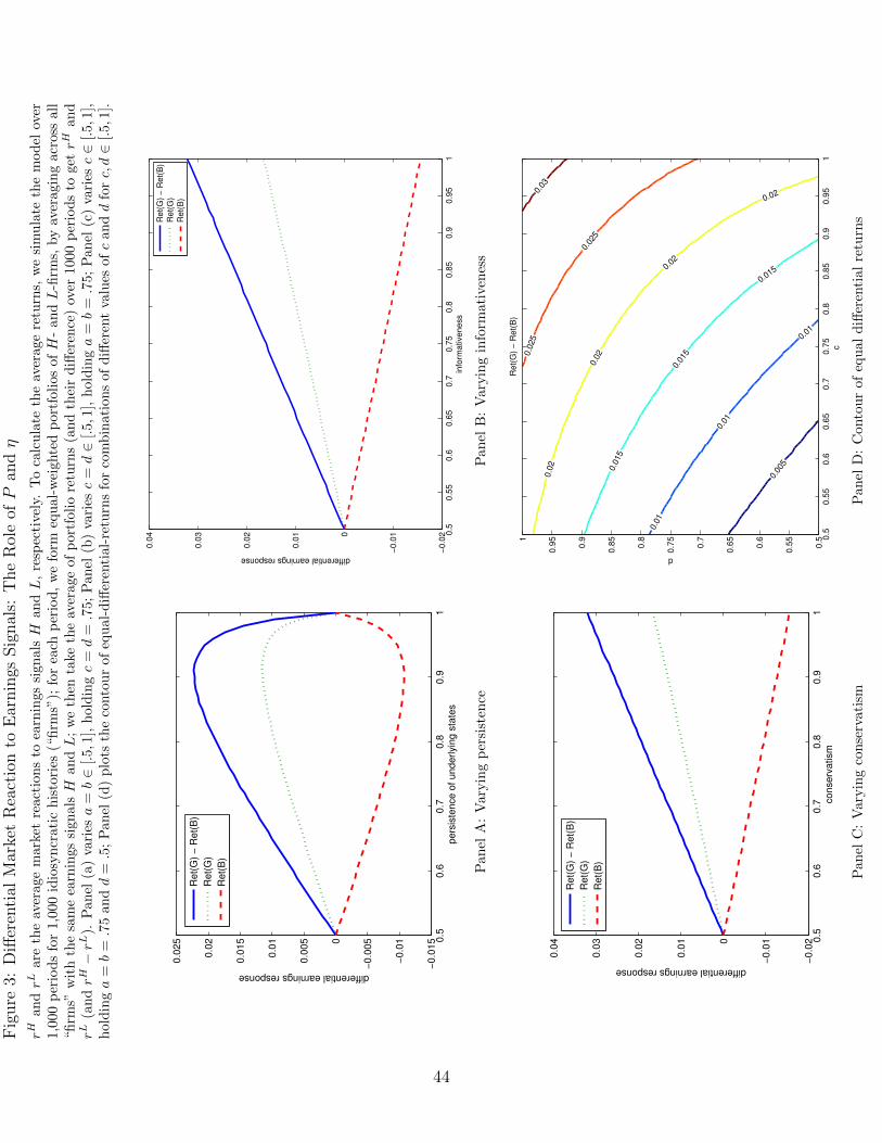
4.1 Average market reactions to earnings signals
To calculate the average returns, we simulate the model over T = 100 periods for N =
10, 000 idiosyncratic histories (“firms”)7. We calibrate the three nonessential parameters as
(L,H, δ) = (1, 2, .06), which will be maintained throughout the simulation analysis8. For
each period, we form equal-weighted portfolios of H- and L-firms, by averaging across all
“firms” with the same earnings signals H and L; we then take the average of portfolio returns
(and their difference) over 1,000 periods to get the average market reactions (stock returns)
to earnings signals H and L and their difference, rH , rL, and rH − rL respectively.
Figure 3 presents the results. When we vary the persistence of underlying state, the
differential reaction first increases then decreases (Panel (a)). The differential reaction in-
creases with both informativeness and conservatism (Panels (b) and (c)). This pattern is
also evident in Panel (d), the contour plot in which both c and d vary from .5 to 1.
4.2 Market reaction to breaks in earnings strings
Prior studies have documented a strong negative market reaction to a break in a string
of consecutive earnings increases (e.g., Barth et al. 1999; Ke et al. 2003). For example, Ke
et al. (2003) document a mean abnormal return is -1.77% for the three-trading-day window
[-2,1] and -4.29% for the 32-trading-day [-30,1] window relative to the announcement of a
break. We revisit this regularity by examining how the length of the string and parameters
of the transition matrix and AIS affect the market reaction to breaks.
7In order to determine M(t), we will need to specify the initial belief M(0). The choice of initial beliefwill not affect the simulation analysis given long enough histories simulated.
8The qualitative patterns of the results are not sensitive the choice of these variables.
19

To calculate the market reaction to breaks, we simulate the model over T periods9 for
N idiosyncratic histories (“firms”). We define a sequence of consecutive good signals as a
“string”, which follows a bad signal and is followed by a bad signal. For example, a string of
length 3 looks like “...LHHHL...”. For each period, we form an equal-weighted portfolio of
all firms with a L signal following exactly s consecutive H signals, where s=1, 2, ..., 8 is the
length of earnings strings. We plot the average of portfolio returns (and their difference) over
1,000 periods for different lengths of the earnings strings. Panel (a) of Figure 4 shows that
the longer the string, the more negative is the reaction, but the effect of increased length on
amplifying the market reaction diminishes as the length increases.
We compare the model prediction with real data. We measure actual reaction as the
average reaction to breaks of earnings strings of lengths 1 to 8, based on a sample of 1,143,863
firm-quarters over 1963-2013 on Compustat, after excluding firms with fiscal year changes.
Earnings strings are defined as consecutive earnings increases, where “earnings increase” is
defined as earnings per share (EPS) before extraordinary items in the observation quarter
being higher than EPS for the same quarter of the previous year. Earnings announcement
return is measured as the cumulative abnormal return starting 2 trading days before to 1
trading day after the earnings announcement date, where returns are adjusted by value-
weighted market or risk, which is measured by market beta estimated using daily returns
of the previous month. We find that the predicted pattern and actual pattern are similar
(Panel (b) of Figure 4).
Figure 5 simulates the market reaction to string breaks for alternative parameter values
9The number of periods is greater than the previous simulation to ensure the existence of a large numberof earnings strings of various lengths, but comes at a cost of computing time.
20

of the transition matrix and AIS. When we vary the persistence of underlying state, the
market reaction first decreases then increases (Panel (a)). This is due to the diminishing
weight investors assign to the accounting signal as persistence increases from .5 to 1: When
persistence close to 1, investors put little weight on the break signal (L), which they attribute
to noise in the AIS. Therefore, they do not revise their expectation downward by a lot. The
reaction decreases with both informativeness and conservatism (Panels (b) and (c)). This
is intuitive because more informative/conservative AIS makes investors react more strongly
negative to a bag signal which they believe is less likely to be due to noise. This pattern is
also evident in Panel (d), the contour plot in which both c and d vary from .5 to 1.
4.3 Dual Information Systems
The setting with dual information systems shed lights on empirical findings that involve
the comparison between two reported numbers, such as accruals (earnings vs. cash flows)
and book-tax differences. In the following, we discuss how the model can offer testable
predictions regarding each.
4.3.1 The accruals anomaly
The accruals component of earnings negatively predicts future returns (Sloan 1996).
Researchers have proposed various explanations for the accruals anomaly, including investor
fixation on accruals (e.g., Sloan 1996), earnings persistence (e.g., Richardson et al. 2005),
and investment (e.g., Wu et al. 2010). By incorporating both earnings and cash flows, our
model of AIS and investors’ Bayesian learning may be able to yield new insights on factors
underlying the return predictability based on accruals. Let the dual information systems
21

correspond to earnings and cash flows, respectively: < X, Y, Z, ηE, ηCF > for every state xt,
ηE generates an earnings signal yt, and ηCF generates a cash flow signal zt, where
Our main variables of interest are the relative informativeness and relative conservatism
of cash flows compared with earnings. Accruals are defined as the difference between earnings
and cash flows, i.e.,
Accrualst = yt − zt ∈ {−(H − L), 0, (H − L)}. (4.1)
To study the accruals anomaly, we simulate N idiosyncratic firms for T periods, and form
portfolios based on the level of accruals, Accrualst. Specifically, for each period, we form a
zero-investment portfolio by buying all firms with negative accruals in the previous period
(i.e., Accrualst−1 = −(H − L)) and shorting all firms with positive accruals in the previous
period (i.e., Accrualst−1 = H − L). We use the equal-weighted returns as portfolio return.
The existence of accruals anomaly would be indicated by a positive return to the hedge
portfolio over some forecasting horizon.
Figure 6 reports the simulation results. Panel A reports the return to an average hedging
portfolio formed based on the accruals τ periods earlier, where τ = 1, 2, ..., 7 is on the x-
axis. The parameters are (a, b, cE, dE, cCF, dCF) = (.75, .75, .75, .75, .6, .6). Panels B, C, and
D report the variations of the one-period ahead accruals-based portfolio returns with respect
to: (B) the persistence of the state process, i.e., a = b ∈ [.5, .95], for (cE, dE, cCF, dCF) =
(.75, .75, .6, .6); (C) the relative informativeness of cash flows, i.e., ∆ = cCF−cE = dCF−dE ∈
[−.25, .25], for (a, b, cE, dE) = (.75, .75, .75, .75); and (D) the relative conservatism of cash
flows, i.e., ∆ = cCF − cE = dE − dCF ∈ [0, .25], for (a, b, cE, dE) = (.75, .75, .75, .75).
Figure 6 shows that when cash flows are less informative about the underlying states
22

than earnings (which is consistent with the central tenet of the accrual-based accounting),
the accruals anomaly exists. Panel A reports the buy-and-hold return to an average hedging
portfolio formed at a certain period based on the accruals of the last period, and held for
τ = 1, 2, ..., 7 periods. The return predictability diminishes as we hold the portfolios for
more periods into the future. The accruals anomaly first increases but then decreases as
the underlying state process is more persistent (Panel B); it decreases with the relative
informativeness and conservatism of cash flows benchmarked against earnings (Panels C and
D).
Panel C suggests that the accruals anomaly only exists when cash flows are less informa-
tive than earnings about the underlying states. This is consistent with the basic notion that
net income is considered a better indicator of future operating cash flows than is current net
operating cash flow (Spiceland et al. 2013, p.7).
Over time, the accruals anomaly has become less significant (Green et al. 2011). Based
on our model prediction, this could be explained by the increasing relative informativeness
of cash flows relative to earnings, which have been shown to be lower quality in recent years,
partially due to large numbers of write-offs and other one-time items.
4.3.2 Book-tax differences (BTDs) and future stock returns
Prior studies document that return predictability based on book-tax differences (e.g., Lev
and Nissim 2006). Our model can also shed light on how BTDs predict future stock returns.
Let the dual information systems correspond to book income (earnings) and taxable income,
respectively: < X, Y, Z, ηBook, ηTax > for every state xt, ηBook generates an earnings signal
yt, and ηTax generates a cash flow signal zt.
23

A higher BTD relative to other firms indicates that taxable income is more conservative
than book income, which could be due to either lower conservatism in book income (Pratt
2005)10 or greater conservatism in taxable income (Heltzer 2009). To the extent that more
conservative tax income also partially means more informative tax income relative to book
income, the model predicts that BTDs are positively associated with future stock returns.
5 Concluding Remarks
This paper proposes a framework for understanding the role of AIS in accounting-based
stock return regularities. The model generate predictions on the market reactions to ac-
counting signals and return predictabilities which are consistent with a battery of empirical
regularities on the relationship between accounting information and stock returns.
There are several limitations to the current framework. First, this paper does not address
the discretionary reporting decisions. Instead, our focus is to study the properties and
implications of an exogenous AIS. Second, even though the Bayesian belief of investors is
consistent various empirical regularities, we acknowledge that other schemes of learning,
including seemingly irrational beliefs such as , such as limited memory and regime-shifting
beliefs (e.g., Barberis et al. 1998), may also produce empirical regularities.
10This statement is based on the assumption that book income is more susceptible to reporting discretion.As Pratt (2005) notes, “the extent to which reported income before taxes exceeds (or is less than) taxableincome indicates how conservative reported income is. Ratios (of reported book income before taxes totaxable income) around 1 or less indicate relatively conservative levels, while reported income becomesincreasingly less conservative as the ratio grows.”
24

Appendix A. General Model Setup
In Appendix A, we extend the 2 by 2 case to more general cases with nx states and ny
(and nz) signals.
A.1 Single Accounting Information System
Suppose a firm’s underlying state (e.g., profitability) xt can take one of the nx values
from X, the set of all possible states by X = {Xi : i = 1, ..., nx}. The law of motion for xt
is described by a Markov transition matrix P = (Pij)nx×nx with
Pij = Pr(xt+1 = Xj|xt = Xi) (A.1)
The sum of each row of P is 1, namely,∑nx
j=1 Pij = 1.
Following Marschak and Miyasawa (1968) and Marschak (1971), we introduce accounting
information system as < X, Y, η >, where Y = {Yi : i = 1, ..., ny} is the set of possible signals,
and η is a measurement matrix which maps the states to accounting signals. After observing
state xt, a firm manager use the accounting information system to generate a signal yt ∈ Y ,
which is a noisy function of xt. AIS can be described by η = (ηij)nx×ny , where
ηij = Pr(yt = yj|xt = xi) (A.2)
The sum of each row of η is 1, namely,∑ny
j=1 ηij = 1. We assume Xi and Yi are in ascending
order with respect to the subscript.
Some special cases of the information system are easy to define. An information system
η is said to be a null information system if its rows are identical, i.e., ηij = ζj for all i, where∑ny
j=1 ζj = 1; when nx = ny, η is said to be a perfect information system if η is a permutation
matrix.
Denote investor belief at t by M(t) = [M1(t), ..., Mnx(t)]′, where Mi(t) = Pr{xt =
Xi|yt}, yt = {yt, ..., y0} is the history of accounting signals. The following proposition
characterizes the law of motion for investor beliefs.
Lemma A.1 Upon observing yt+1 = yj, an investor’s belief is given by the following
25

recursive formula:
M(t+ 1) =M(t+ 1)
M(t+ 1) · 1(A.3)
where M(t+ 1) ≡ diag(ηj)P′M(t), ηj = [η1j, ..., ηnxj]
′ is the j-th column of η.
A.2 Dual Information Systems
Suppose the underlying state xt is imperfectly revealed by an information system with
two information channels, < X, Y, Z, η1, η2 > for every state xt, η1 generates a signal yt, and
η2 generates a different signal zt ∈ Z, where Z = {Zi : i = 1, ..., nz} and Zi are in ascending
order with respect to the subscript.
Lemma A.2 Upon observing yt+1 = Yj and zt+1 = Zk, an investor’s belief is given by the
following recursive formula:
M(t+ 1) =M(t+ 1)
M(t+ 1) · 1(A.4)
where M(t+ 1) ≡ diag(η1j ◦ η2
k)P′M(t), with η1
j = [η11j, ..., η
1nxj]
′ being the j-th column of η1
and η2k = [η2
1k, ..., η2nxk
]′ being the k-th column of η2. Here, η1j ◦ η2
k denotes their Hadamard
Product.
A.3 Stock Prices
Interpreting xt as the underlying cash flows of period t, the post-accounting-signal price
is the cum-dividend price, pt is given by the following lemma.
Lemma A.3 After observing accounting signals in each period t, stock price pt is given by
pt = M ′t
(I − 1
1 + δP)−1
X (A.5)
where δ is the discount rate and I is the identity matrix of size nx, and X is the vector of
possible values for xt ordered by subscripts.
26

Appendix B: Proofs
Proof of Lemma 1.
For brevity, we only prove the expression for µt|yt=L. µt|yt=H can be derived analogously.
By Bayes’ Rule,
µt|yt=L = Pr(xt = B|yt = L,yt−1)
=Pr(yt = L|xt = B)Pr(xt = B|yt−1)
Pr(yt = L|xt = B,yt−1)
=
∑xt−1=B,G Pr(yt = L|xt = B)Pr(xt = B|xt−1)Pr(xt−1|yt−1)∑xt=B,G
∑xt−1=B,G Pr(yt = L|xt)Pr(xt|xt−1)Pr(xt−1|yt−1)
=caµt−1 + c(1− b)(1− µt−1)
(caµt−1 + c(1− b)(1− µt−1)) + ((1− d)(1− a)µt−1 + (1− d)b(1− µt−1))
=c(a+ b− 1)µt−1 + c(1− b)
(c+ d− 1)(a+ b− 1)µt−1 + (1− d)b+ c(1− b)(B.1)
Proof of Proposition 1. For notational brevity, let gL(µ) and gH(µ) denote the belief
updating functions given the belief from last period being µt = µ:
gL(µ) = µt+1|yt+1=L,µt=µ (B.2)
gH(µ) = µt+1|yt+1=H,µt=µ (B.3)
Suppose Conditions 1-2 are met, i.e., a + b ≥ 1 and c + d ≥ 1. It is straightforward to
show that both gL(µ) and gH(µ) are increasing functions for µ ∈ [0, 1]:
g′L =c(1− d)(a+ b− 1)
(c((a− 1)µ+ 1) + (a− 1)(d− 1)µ+ b(µ− 1)(c+ d− 1))2≥ 0 (B.4)
g′H =(1− c)d(a+ b− 1)
(acµ+ adµ− aµ+ b(µ− 1)(c+ d− 1)− cµ+ c− dµ+ µ− 1)2≥ 0 (B.5)
Additionally, we can show that gL(µ) is a concave function for µ ∈ [0, 1], i.e.,
g′′L =2c(d− 1)(a+ b− 1)2(c+ d− 1)
(c((a− 1)µ+ 1) + (a− 1)(d− 1)µ+ b(p− 1)(c+ d− 1))3≤ 0; (B.6)
and that gH(µ) is a convex function for µ ∈ [0, 1], i.e.,
g′′H(µ) =2(c− 1)d(a+ b− 1)2(c+ d− 1)
(acµ+ adµ− aµ+ b(µ− 1)(c+ d− 1)− cµ+ c− dµ+ µ− 1)3≥ 0. (B.7)
27

It is also easy to show that gL(µ) ≥ µ is equivalent to
0 ≤ µ ≤ µ (B.8)
where µ = 12
(√c(a2c+4a(d−1)−4d+4)−2(a−2)bc(d−1)+b2(d−1)2
(a+b−1)2(c+d−1)2+ (a−2)c+b(2c+d−1)
(a+b−1)(c+d−1)
). and that gH(µ) ≤
µ is equivalent to
µ ≤ µ ≤ 1 (B.9)
where µ = 12
(a(c−1)+b(2c+d−2)−2c+2
(a+b−1)(c+d−1)−√
a2(c−1)2−2a(b−2)(c−1)d+d(b2d+4b(c−1)−4c+4)(a+b−1)2(c+d−1)2
). It is also easy
to show that µ ≤ µ holds.
Therefore, for ∀µ ∈ [µ, µ], we have µ ≤ gL(µ) ≤ µ and µ ≤ gH(µ) ≤ µ. In other words,
if we start from µt ∈ [µ, µ], µt+1 will always stay within the range [µ, µ].
For ∀µ ∈ [0, µ), we have gL(µ) > µ and gH(µ) > µ. In other words, if we start from
µt ∈ [0, µ), µt+1 will eventually rise to the range [µ, µ].
For ∀µ ∈ (µ, 1], we have gL(µ) < µ and gH(µ) < µ. In other words, if we start from
µt ∈ (µ, 1], µt+1 will eventually fall to the range [µ, µ].
Proof of Corollary 1. Omitted for brevity. It can be easily verified by checking the sign
of the derivatives given Conditions 1 and 2.
Proof of Lemma 2. For brevity, we only prove the expression for µt|yt=L,zt=L. By Bayes’
Rule,
µt|yt=L,zt=L = Pr(xt = B|yt = L, zt = L,yt−1, zt−1)
=Pr(yt = L, zt = L|xt = B)Pr(xt = B|yt−1, zt−1)
Pr(yt = L, zt = L|xt = B,yt−1, zt−1)
=
∑xt−1=B,G Pr(yt = L, zt = L|xt = B)Pr(xt = B|xt−1)Pr(xt−1|yt−1)∑xt=B,G
∑xt−1=B,G Pr(yt = L, zt = L|xt)Pr(xt|xt−1)Pr(xt−1|yt−1)
=c1c2aµt−1 + c1c2(1− b)(1− µt−1)
(c1c2aµt−1 + c1c2(1− b)(1− µt−1)) + ((1− d1)(1− d2)(1− a)µt−1 + (1− d1)(1− d2)b(1− µt−1))
=c1c2((a+ b− 1)µt−1 + 1− b)
c1c2((a+ b− 1)µt−1 + 1− b) + (1− d1)(1− d2)((1− a− b)µt−1 + b)(B.10)
The proofs for the other three scenarios (µt|yt=L,zt=H , µt|yt=H,zt=L, and µt|yt=H,zt=H) are
analogous.
Proof of Proposition 2. Define gij(µ) ≡ µt+1|yt+1=i,zt+1=j,µt=µ, where i, j ∈ {L,H}.
28

It is easy to show that given Conditions 1 and 3, i.e., for (a, b, c1, d1, c2, d2) such that
a, b, c1, d1, c2, d2 ∈ (0, 1), a + b > 1, c1 + d1 > 1 and c2 + d2 > 1, the following two in-
equalities always hold:
gHH(µ) < gLH(µ) < gLL(µ) (B.11)
gHH(µ) < gHL(µ) < gLL(µ) (B.12)
Therefore, in order to bound the value of µt, we only need to consider the bounds of
gLL(µ) and gHH(µ).
We can show that gLL(µ) ≥ µ is equivalent to
0 ≤ µ ≤ µ∗∗ (B.13)
where µ∗∗ is given by (2.11), and that gHH(µ) ≤ µ is equivalent to
µ∗ ≤ µ ≤ 1 (B.14)
where µ∗ is given by (2.10). These conditions ensure that if yt+1 = L and zt+1 = L, then
µt+1 ≥ µt; if yt+1 = H and zt+1 = H, then µt+1 ≤ µt.
It is also easy to show that the second order conditions for concavity/convexity are met.
For ∀a, b, c, d such that Conditions 1 and 3 are met, we have
g′′LL(µ) = −2c1c2(d1 − 1)(d2 − 1)(a+ b− 1)2(c1c2 − d1d2 + d1 + d2 − 1)
(c1c2((a− 1)µ+ 1)− (a− 1)(d1 − 1)(d2 − 1)µ+ b(p− 1)(c1c2 − d1d2 + d1 + d2 − 1))3≤ 0 (B.15)
g′′HH(µ) =2(c1 − 1)(c2 − 1)d1d2(a+ b− 1)2(c1(−c2) + c1 + c2 + d1d2 − 1)
(c1(c2 − 1)((a− 1)µ+ 1)− ac2µ− ad1d2µ+ ap+ b(µ− 1)(c1(c2 − 1)− c2 − d1d2 + 1) + c2µ− c2 + d1d2µ− µ+ 1)3
≥ 0 (B.16)
The rest of the proof is analogous to that of Proposition 1.
Proof of Corollary 2. Analogous to that of Corollary 1.
Proof of Lemma 3. The risk-neutral cum-dividend price is equal to the discounted ex-
pected future cash flows. Given that that 11+δ
< 1 ensures the convergence of I + 11+δ
P +
1(1+δ)2
P 2 + ... = (I − 11+δ
P )−1, we have
pt = (µt, 1− µt)(I − 1
1 + δP
)−1
X (B.17)
29

where X = (B,G)′.
Equation (B.17) can be easily rewritten as
pt =1 + δ
δ(2− a− b+ δ)
(G(1− a+ δ) +B(1− b)− δ(G−B)µt
). (B.18)
Proof of Lemma 4. For a Bayesian investor, equation (3.1) follows directly from the fact
that Eit [µt] = µt. To prove equation (3.2), we need to derive an expression for Ei
t [µt+1|µt].
Note that
Eit [µt+1|µt] = Pr(yt+1 = L|µt) · µt+1|yt+1=L + Pr(yt+1 = H|µt) · µt+1|yt+1=H (B.19)
where
Pr(yt+1 = L|µt) =∑
xt+1∈{B,G}
∑xt∈{B,G}
Pr(yt+1 = L|xt+1)Pr(xt+1|xt)Pr(xt|µt)
=(µta+ (1− µt)(1− b)
)c+
(µt(1− a) + (1− µt)b
)(1− d) (B.20)
Pr(yt+1 = H|µt) =∑
xt+1∈{B,G}
∑xt∈{B,G}
Pr(yt+1 = L|xt+1)Pr(xt+1|xt)Pr(xt|µt)
=(µta+ (1− µt)(1− b)
)(1− c) +
(µt(1− a) + (1− µt)b
)d (B.21)
µt+1|yt+1=L =c(a+ b− 1)µt + c(1− b)
(c+ d− 1)(a+ b− 1)µt + (1− d)b+ c(1− b)(B.22)
µt+1|yt+1=H =(1− c)(a+ b− 1)µt + (1− c)(1− b)
(1− c− d)(a+ b− 1)µt + db+ (1− c)(1− b)(B.23)
It follows that
Eit [µt+1|µt] = aµt + (1− b)(1− µt). (B.24)
Based on equation (2.13), it is straightforward to show that the expected price change from
an investor’s perspective is:
Eit [pt+1 − pt] =
1 + δ
2− a− b+ δ(G−B)
((2− a− b)µt − 1 + b
)(B.25)
For an empiricist, the expectation of current period belief is
Eet [µt] =
∫µt
µtdF (µt) = πB =1− b
2− a− b(B.26)
30

Therefore,
Eet [pt] =
1 + δ
δ(2− a− b+ δ)
(G(1− a+ δ) +B(1− b)− δ(G−B)πB
)(B.27)
Eet [pt+1 − pt] =
1 + δ
2− a− b+ δ(G−B)
((2− a− b)πB − 1 + b
)= 0 (B.28)
Proof of Proposition 3.
Eet [pt|yt = H]− Ee
t [pt|yt = L] = − 1 + δ
2− a− b+ δ(G−B)
(Et[µt|yt = H]− Et[µt|yt = L]
)= − 1 + δ
2− a− b+ δ(G−B)
∫µt−1
(µt|yt=H − µt|yt=L
)dF (µt−1)
≥ 0 (B.29)
The last inequality obtains because the integrand is negative for µt−1 ∈ (µ, µ).
Proof of Proposition 4. Suppose the earnings string is of length s = 1, i.e., yt = L, yt−1 =
H. The conditional expectation of price change for an empiricist is
Eet [pt − pt−1|yt = L, yt−1 = H]
=− 1 + δ
2− a− b+ δ(G−B)Ee
t [µt − µt−1|yt = L, yt−1 = H]
=− 1 + δ
2− a− b+ δ(G−B)
∫µt−1
(gL(µt−1)− µt−1
)dF (µt−1|yt−1 = H)
≤0 (B.30)
because gL(µt−1) ≥ µt−1 for µt−1 ∈ [µ, µ].
Suppose the earnings string is of length s = 2, i.e., yt = L, yt−1 = yt−2 = H. The
conditional expectation of price change for an empiricist is
Eet [pt − pt−1|yt = L, yt−1 = yt−2 = H]
=− 1 + δ
2− a− b+ δ(G−B)Ee
t [µt − µt−1|yt = L, yt−1 = yt−2 = H]
=− 1 + δ
2− a− b+ δ(G−B)
∫µt−1
(gL(µt−1)− µt−1
)dF (µt−1|yt−1 = yt−2 = H) (B.31)
≤0 (B.32)
31

Now we would like to find conditions for
Eet [pt − pt−1|yt = L, yt−1 = H] ≥ Ee
t [pt − pt−1|yt = L, yt−1 = yt−2 = H] (B.33)
This is equivalent to∫µt−1
(gL(µt−1)− µt−1) dF (µt−1|yt−1 = H) ≤∫µt−1
(gL(µt−1)− µt−1) dF (µt−1|yt−1 = yt−2 = H)
(B.34)
Define FH(µt−1) = F (µt−1|yt−1 = H) and FHH(µt−1) = F (µt−1|yt−1 = yt−2 = H). By
integration by parts, the left hand side of (B.34) is∫µt−1
(gL(µt−1)− µt−1) dF (µt−1|yt−1 = H)
= (gL(µ)− µ)︸ ︷︷ ︸=0
FH(µ)︸ ︷︷ ︸=1
−(gL(µ)− µ
)FH(µ)︸ ︷︷ ︸
=0
−∫ µ
µ
FH(µt−1) (g′L(µt−1)− 1) dµt−1
=−∫ µ
µ
(g′L(µt−1)− 1)FH(µt−1)dµt−1 (B.35)
Similarly, the right hand side is∫µt−1
(gL(µt−1)− µt−1) dF (µt−1|yt−1 = yt−2 = H) = −∫ µ
µ
(g′L(µt−1)− 1)FHH(µt−1)dµt−1
(B.36)
Therefore, inequality (B.34) becomes∫ µ
µ
(g′L(µt−1)− 1)FH(µt−1)dµt−1 ≥∫ µ
µ
(g′L(µt−1)− 1)FHH(µt−1)dµt−1 (B.37)
A sufficient condition for (B.36) is
(g′L(µt−1)− 1)FH(µt−1) ≥ (g′L(µt−1)− 1)FHH(µt−1) (B.38)
for ∀µt−1. In the following, we first prove
FH(µt−1) ≤ FHH(µt−1), (B.39)
and derive a sufficient condition for the above inequality to hold.
32

By definition, for a given µt−3,
FH(µt−1) =F (µt−1|yt−1 = H) = Pr(gH(µt−2) ≤ µt−1) = Pr(µt−2 ≤ g−1H (µt−1))
=γPr(gL(µt−3) ≤ g−1H (µt−1)) + (1− γ)Pr(gH(µt−3) ≤ g−1
H (µt−1)) (B.40)
where γ = Pr(yt−2 = L);
FHH(µt−1) =F (µt−1|yt−1 = yt−2 = H) = Pr(gH(gH(µt−3)) ≤ µt−1)
=Pr(gH(µt−3) ≤ g−1H (µt−1)) (B.41)
Because gL(µt−3) ≥ gH(µt−3) for ∀µt−3, it follows that
Pr(gL(µt−3) ≤ g−1H (µt−1)) ≤ Pr(gH(µt−3) ≤ g−1
H (µt−1)) (B.42)
and therefore
FH(µt−1) ≤ FHH(µt−1) (B.43)
for ∀µt−1 ∈ [µ, µ]. In other words, FH first-order stochastically dominates (f.o.s.d.) FH .
Given (B.43), a sufficient condition for (B.38) to hold is
g′L(µt−1)− 1 ≤ 0. (B.44)
for ∀µt−1. It is easy to show that (B.44) is met when either of the following two conditions
(in addition to Conditions 1 and 2) is true:
(i) 0 ≤ b ≤ b∗, where b∗ =c(
(2c+d−1)−√
(1−d)(4c+3d−3))
2(c+d−1)2;
(ii) b∗ ≤ b ≤ 1 and 0 ≤ a ≤ a∗, where a∗ = b2(c+d−1)2−bc(2c+d−1)+c(c−d+1)c(1−d)
;
Now let us consider longer earnings strings. Note that based on the proof of (), analogous
arguments for longer sequences of H signals can be proved by induction. For example, FHH
first-order stochastically dominates (f.o.s.d.) FHHH , and so forth. As the earnings string
becomes infinitely long, we have
lims→∞
µt−1 = µ (B.45)
and
lims→∞
FHH...H(µt−1) = 1 (B.46)
33

As a result,
lims→∞
Eet [pt − pt−1|yt = L, yt−1 = ... = yt−s = H] = Ee
t [pt − pt−1|yt = L, µt−1 = µ]
=− 1 + δ
2− a− b+ δ(G−B)
( c(a+ b− 1)µ+ c(1− b)(c+ d− 1)(a+ b− 1)µ+ (1− d)b+ c(1− b)
− µ)
(B.47)
Analogously, if the investor observes a sequence of bad news before seeing a break, the
market reaction will be
lims→∞
Eet [pt − pt−1|yt = H, yt−1 = ... = yt−s = L] = Ee
t [pt − pt−1|yt = H,µt−1 = µ]
=− 1 + δ
2− a− b+ δ(G−B)
( (1− c)(a+ b− 1)µ+ (1− c)(1− b)(1− c− d)(a+ b− 1)µ+ db+ (1− c)(1− b)
− µ)
(B.48)
Proof of Proposition 5. Recall the price change is given by
pt+1 − pt = − 1 + δ
2− a− b+ δ(G−B)(µt+1 − µt). (B.49)
where µt+1 is given by (2.3) and (2.4). Before we derive the expression for ht, it is useful to
observe
Prob(yt+1 = H|yt = H) =∑
xt+1∈{B,G}
∑xt∈{B,G}
Prob(yt+1 = H|xt+1)Prob(xt+1|xt)Prob(xt|yt = H)
= µt(a(1− c) + (1− a)d) + (1− µt)(bd+ (1− b)(1− c))
= (µta+ (1− µt)(1− b))(1− c) + (µt(1− a) + (1− µt)b)d (B.50)
Prob(yt+1 = L|yt = H) =∑
xt+1∈{B,G}
∑xt∈{B,G}
Prob(yt+1 = L|xt+1)Prob(xt+1|xt)Prob(xt|yt = H)
= µt(ac+ (1− a)(1− d)) + (1− µt)(b(1− d) + (1− b)c)
= (µta+ (1− µt)(1− b))c+ (µt(1− a) + (1− µt)b)(1− d) (B.51)
34

Et(pt+1 − pt|yt = H,µt = µ)
=− 1 + δ
2− a− b+ δ(G−B)Et(µt+1 − µt|yt = G, µt = µ)
=− 1 + δ
2− a− b+ δ(G−B)
[(µ[ac+ (1− a)(1− d)] + (1− µ)[b(1− d) + (1− b)c]
)gB(µ)
+(µ[a(1− c) + (1− a)d] + (1− µ)[bd+ (1− b)(1− c)]
)gG(µ)
]=
1 + δ
2− a− b+ δ(G−B)
((2− a− b)µ− 1 + b
)(B.52)
Similarly,
Et(pt+1 − pt|yt = L, µt = µ) =1 + δ
2− a− b+ δ(G−B)
((2− a− b)µ− 1 + b
)(B.53)
Let φ(µ) = 1+δ2−a−b+δ (G − B)
((2 − a − b)µ − 1 + b
). Note that φ(µ) is a linear increasing
function of µ:
φ′(µ) =(1 + δ)(2− a− b)
2− a− b+ δ(G−B) > 0 (B.54)
Therefore,
Eet (pt+1 − pt|yt = H) =
∫µt
φ(µt)dF (µt|yt = H) (B.55)
Eet (pt+1 − pt|yt = L) =
∫µt
φ(µt)dF (µt|yt = L) (B.56)
This is the key to the return predictability: the distribution of µt conditional on signals
are different between L and H.
Note that with probability 1, µt ∈ [µ, µ]. Therefore, evaluating the integration over the
full support of [0, 1] is equivalent to evaluating the integration over [µ, µ]. Denote FH(µt) =
F (µt|yt = H) and FL(µt) = F (µt|yt = L), we know that FH(µ) = FL(µ) = 0 and FH(µ) =
FL(µ) = 1.
∫µt
µtdFH(µt) =
∫ µ
µ
µtdFH(µt) = µ · FH(µ)− µ · FH(µ)−
∫ µ
µ
FH(µt)dµt
= µ−∫ µ
µ
FH(µt)dµt (B.57)
The inequality∫µtµtdF
H(µt) <∫µtµtdF
L(µt) is equivalent to∫ µµFH(µt)dµt ≥
∫ µµFL(µt)dµt.
In the following, we prove a sufficient condition of the above inequality, namely, FH(µt) ≥
35

FL(µt) for ∀µt.
By definition, for a given µt−1,
FH(µ) = F (µt|yt = H) = Pr(gH(µt−1) ≤ µ) (B.58)
FL(µ) = F (µt|yt = L) = Pr(gL(µt−1) ≤ µ) (B.59)
Given that gL(µt−1) ≥ gH(µt−1) for ∀µt−1, it follows that FH(µ) ≥ FL(µ) for ∀µ.
Proof of Corollary 3. Define
h(µ) = φ(µt|yt=H,µt−1=µ
)− φ(µt|yt=L,µt−1=µ
)= φ
(gH(µ)
)− φ(gL(µ)
), (B.60)
It is easy to show that ∂gL(µ)∂c≥ 0 and ∂gH(µ)
∂c≤ 0 for ∀µ. Therefore,
∂h(µ)
∂c=
(1 + δ)(2− a− b)2− a− b+ δ
(G−B)
(∂gH(µ)
∂c− ∂gL(µ)
∂c
)≤ 0 (B.61)
Therefore,
∂h(µ)
∂c=
∂
∂c
∫ µ
µ
h(µ)dF (µ)
= h(µ)︸︷︷︸−
· ∂µ∂c︸︷︷︸+
−h(µ)︸︷︷︸−
·∂µ
∂c︸︷︷︸−
+
∫ µ
µ
∂h(µ)
∂c︸ ︷︷ ︸−
dF (µ) ≤ 0 (B.62)
Similarly, we can prove that
∂h(µ)
∂d≤ 0. (B.63)
Proof of Proposition 6. The hedge return obtained by trading on the two signals is
Eet (pt+1 − pt|yt = H, zt = L)− Ee
t (pt+1 − pt|yt = L, zt = H) (B.64)
Note that
Eet (pt+1 − pt|µt = µ) =
1 + δ
2− a− b+ δ(G−B)
((2− a− b)µ− 1 + b
)≡ φ(µ) (B.65)
Therefore,
Eet (pt+1 − pt|yt = H, zt = L) =
∫µ
φ(µ)dF (µ|yt = H, zt = L) (B.66)
36

Eet (pt+1 − pt|yt = L, zt = H) =
∫µ
φ(µ)dF (µ|yt = L, zt = H) (B.67)
Recall:
µt|yt=H,zt=L =(1− c1)c2((a+ b− 1)µt−1 + 1− b)
(1− c1)c2((a+ b− 1)µt−1 + 1− b) + d1(1− d2)((1− a− b)µt−1 + b),
(B.68)
µt|yt=L,zt=H =c1(1− c2)((a+ b− 1)µt−1 + 1− b)
c1(1− c2)((a+ b− 1)µt−1 + 1− b) + (1− d1)d2((1− a− b)µt−1 + b),
(B.69)
Note that with probability 1, µt ∈ [µ∗, µ∗∗]. Therefore, evaluating the integration over
the full support of [0, 1] is equivalent to evaluating the integration over [µ∗, µ∗∗]. Denote
FHL(µt) = F (µt|yt = H, zt = L) and FLH(µt) = F (µt|yt = L, zt = H), we know that
FHL(µ∗) = FLH(µ∗) = 0 and FHL(µ∗∗) = FLH(µ∗∗) = 1. Therefore, analogous to (), we
have ∫µt
µtdFHL(µt) = µ∗∗ −
∫ µ∗∗
µ∗FHL(µt)dµt (B.70)
The inequality∫µtµtdF
HL(µt) ≥∫µtµtdF
LH(µt), is equivalent to∫ µ∗∗µ∗
FHL(µt)dµt ≤∫ µ∗∗µ∗
FLH(µt)dµt. In the following, we prove a sufficient condition of the above inequality,
namely, FHL(µt) ≤ FLH(µt) for ∀µt.
By definition, for a given µt−1,
FHL(µ) = Pr(µHL(µt−1) ≤ µ) (B.71)
Assume a, b, c1, d1, c2, d2 ∈ [0, 1], a + b ≥ 1, c1 + d1 ≥ 1, and c2 + d2 ≥ 1. It is easy to show
that
µt|yt=H,zt=Lµt−1=µ ≥ µt|yt=L,zt=H,µt−1=µ (B.72)
iff
1− d1 ≤ c1 ≤c2d2(1− d1)
d1(1− d2) + c2(d2 − d1)(B.73)
But we know that ∀µt−1, µHL(µt−1) ≥ µLH(µt−1) given the assumptions. Therefore,
Pr(µHL(µt−1) ≤ µ) ≤ Pr(µLH(µt−1) ≤ µ)
37

Given that φ(µ) is a linear increasing function of µ, we have
Eet (pt+1 − pt|yt = H, zt = L)− Ee
t (pt+1 − pt|yt = L, zt = H) ≥ 0 (B.74)
iff
1− d1 ≤ c1 ≤c2d2(1− d1)
d1(1− d2) + c2(d2 − d1)(B.75)
where it can be shown that 1− d1 ≤ c2d2(1−d1)d1(1−d2)+c2(d2−d1)
always hold.
Proof of Lemma A.1. This is a standard result for the hidden Markov model, and is also
proved in other texts. Using Bayes’ rule,
Mi(t+ 1) =αi(t+ 1)∑nx
i′=1 αi′(t+ 1)
where αi(t + 1) ≡ Pr(yt+1, xt+1 = Xi) is the joint probability of yt+1 and xt+1 = Xi. We
know that
αi(t+ 1) =nx∑k=1
Pr(y1, y2, ..., yt+1, xt+1 = Xi, xt = Xk)
=nx∑k=1
Pr(y1, y2, ..., yt, xt = Xk) · Pr(yt+1, xt+1 = Xi|xt = Xk, y1, y2, ..., yt)
=nx∑k=1
αk(t) · Pr(yt+1, xt+1 = Xi|xt = Xk)
=nx∑k=1
αk(t) · Pr(yt+1|xt+1 = Xi, xt = Xk) · Pr(xt+1 = Xi|xt = Xk)
=nx∑k=1
αk(t) · Pr(yt+1|xt+1 = Xi) · Pr(xt+1 = Xi|xt = Xk) (B.76)
where the third equality is based on the fact that given xt, xt+1 is independent of all xτ ,
τ = 1, ..., t− 1, and hence yτ . In addition, xt+1 is independent of yt because xt is given.
Therefore, upon observing yt+1 = Yj,
Mi(t+ 1) =
∑k ηijPkiMk(t)∑
i′∑
k ηi′jPki′Mk(t)(B.77)
which is equivalent to the matrix form of the posterior.
38

Proof of Lemma A.2. Using Bayes’ rule, we have
Mi(t+ 1) =αi(t+ 1)∑nx
i′=1 αi′(t+ 1)(B.78)
where αi(t+ 1) ≡ Pr(yt+1, zt+1, xt+1 = Xi) is the joint probability of yt+1, zt+1 and xt+1 =
Xi.
We know that
αi(t+ 1) =nx∑k=1
Pr(yt, yt+1, zt, zt+1, xt+1 = Xi, xt = Xk)
=nx∑k=1
Pr(yt, zt, xt = Xk) · Pr(yt+1, zt+1, xt+1 = Xi|xt = Xk,yt, zt)
=nx∑k=1
αk(t) · Pr(yt+1, zt+1, xt+1 = Xi|xt = Xk)
=nx∑k=1
αk(t) · Pr(yt+1, zt+1|xt+1 = Xi, xt = Xk) · Pr(xt+1 = Xi|xt = Xk)
=nx∑k=1
αk(t) · Pr(yt+1|xt+1 = Xi) · Pr(zt+1|xt+1 = Xi) · Pr(xt+1 = Xi|xt = Xk)
(B.79)
where the third equality is based on the fact that given xt, xt+1 is independent of all xτ ,
τ = 1, ..., t − 1, and hence yτ and zτ , and the last equality uses the fact that yt+1 and zt+1
are conditionally independent given xt+1. In addition, xt+1 is independent of yt because xt
is given.
Therefore, upon observing yt+1 = Yj and zt+1 = Zl,
Mi(t+ 1) =
∑k ηijξilPkiMk(t)∑
i′∑
k ηi′jξi′lPki′Mk(t)(B.80)
which is equivalent to the matrix form of the posterior.
Proof of Lemma A.3. See the proof of Lemma 3.
39

References
[1] Antle, R., J. Demski, and S. Ryan. 1994. Multiple sources of information, valuation, and
accounting earnings. Journal of Accounting, Auditing and Finance 9, 675-696.
[2] Antle, R., and R. Lambert. 1988. Accountants’ loss functions and induced incentives
for conservatism. In Economic Analysis of Information and Contracts: Essays in Honor
of John Butterworth, edited by G. Feltham, A. Amershi, and W. Ziemba. Boston, MA:
Kluwer Academic Publishers.
[3] Barberis, N., A. Shleifer, and R. Vishny. 1998. A model of investor sentiment. Journal of
Financial Economics 49, 307-345.
[4] Barth, M. E., J. A. Elliott, and M. W. Finn. 1999. Market rewards associated with
patterns of increasing earnings. Journal of Accounting Research 37, 387-413.
[5] Berger, J. 1985. Statistical Decision Theory and Bayesian Analysis. New York: Springer-
Verlag.
[6] Blackwell, D. 1953. Equivalent comparisons of experiments. Annals of Mathematical
Statistics, 24, 265-72.
[7] Christensen, J., and J. Demski. 2003. Accounting Theory: An Information Content Per-
spective. McGraw-Hill/Irwin.
[8] Demski, J. 1973. The general impossibility of normative accounting standards. The Ac-
counting Review 48, 718-723.
[9] Gigler, F., C. Kanodia, H. Sapra, and R. Venugopalan. 2009 Accounting conservatism
and the efficiency of debt contracts. Journal of Accounting Research 47, 767-797.
[10] Heltzer, W. 2009. Conservatism and Book-Tax Differences. Journal of Accounting, Au-
diting and Finance 24, 469-504.
[11] Ke, B., S. Huddart, and K. Petroni. 2003. What insiders know about future earnings
and howthey use it: Evidence from insider trades. Journal of Accounting and Economics
35, 315-346.
[12] Kothari, S.P. 2001. Capital market research in accounting. Journal of Accounting Eco-
nomics 31, 105-231.
[13] Lev, B., and D. Nissim. 2004. Taxable income, future earnings, and equity values. The
Accounting Review 79, 1039-1074.
[14] Lewellen, J., and J. Shanken. 2002. Learning, asset-pricing tests, and market efficiency.
Journal of Finance 57, 1113-1145.
40

[15] Marschak, J. 1971. Economics of information systems. Journal of the American Statis-
tical Association 66, 192-219.
[16] Marschak, J., and K. Miyasawa. 1968. Economic comparability of information systems.
International Economic Review 9, 137-174.
[17] Pratt, J. 2005. Financial Accounting in an Economic Context. 6th ed. Hoboken, NJ:
John Wiley & Sons.
[18] Richardson, S., R. Sloan, M. Soliman, and I. Tuna. 2005. Accrual reliability, earnings
persistence and stock prices. Journal of Accounting and Economics 39, 437-485.
[19] Richardson, S., I. Tuna, and P. Wysocki. 2010. Accounting anomalies and fundamental
analysis: A review of recent research advances. Journal of Accounting and Economics
50, 410-454.
[20] Scott, W. 1979. Scoring Rules for Probabilistic Reporting. Journal of Accounting Re-
search 17, 156-178.
[21] Sloan, R. 1996. Do stock prices fully reflect information in accruals and cash flows about
future earnings? The Accounting Review 71, 289-315.
[22] Spiceland, J., J. Sepe, and M. Nelson. 2013. Intermediate Accounting. 7th ed. New York,
NY: McGraw-Hill Irwin.
[23] Wu, J., L. Zhang, and X. Zhang. 2010. The q-theory Approach to Understanding the
Accrual Anomaly. Journal of Accounting Research 48, 177-223.
41

Figure 1: Accounting Information System
Panel A illustrates the time-series structure of the model. Panel B illustrates the law of motion (a Markovprocess) for the underlying state xt and the information system which maps the state to an accounting signalyt.
xt−1 xt xt+1
yt−1 yt yt+1
(a) The time-series structure of the model
B L
G H
c
1−c
1−d
d
a
b
1− a 1− b
(b) The law of motion for xt and the information system
42

Figure 2: Dual Accounting Information Systems
Panel A illustrates the time-series structure of the two-AIS model. Panel B illustrates the law of motion(a Markov process) for the underlying state xt and the information systems which map the state to anaccounting signals yt and zt.
xt−1 xt xt+1
yt−1 yt yt+1
zt−1 zt zt+1
(a) The time-series structure of the model
B LL
G HH
c1
1−c1
1−d 1
d1
c2
1−c 2
1−d2
d2
a
b
1− a 1− b
(b) The law of motion for xt and the information system43
Fig
ure
3:D
iffer
enti
alM
arke
tR
eact
ion
toE
arnin
gsSig
nal
s:T
he
Rol
eofP
andη
rHan
drL
are
the
aver
age
mar
ket
reac
tion
sto
earn
ings
sign
alsH
an
dL
,re
spec
tive
ly.
To
calc
ula
teth
eav
erage
retu
rns,
we
sim
ula
teth
em
od
elov
er1,
000
per
iod
sfo
r1,
000
idio
syn
crat
ich
isto
ries
(“fi
rms”
);fo
rea
chp
erio
d,
we
form
equ
al-
wei
ghte
dp
ort
foli
os
ofH
-an
dL
-firm
s,by
aver
agin
gacr
oss
all
“firm
s”w
ith
the
sam
eea
rnin
gssi
gnal
sH
andL
;w
eth
enta
keth
eav
erage
of
port
foli
ore
turn
s(a
nd
thei
rd
iffer
ence
)ov
er1000
per
iod
sto
getrH
an
drL
(an
drH−rL
).P
anel
(a)
vari
esa
=b∈
[.5,
1],
hold
ingc
=d
=.7
5;
Pan
el(b
)va
riesc
=d∈
[.5,
1],
hold
inga
=b
=.7
5;
Panel
(c)
vari
esc∈
[.5,
1],
hol
din
ga
=b
=.7
5an
dd
=.5
;P
anel
(d)
plo
tsth
eco
nto
ur
of
equ
al-
diff
eren
tial-
retu
rns
for
com
bin
ati
on
sof
diff
eren
tva
lues
ofc
an
dd
forc,d∈
[.5,
1].
0.5
0.6
0.7
0.8
0.9
1−
0.0
15
−0.0
1
−0.0
050
0.0
05
0.0
1
0.0
15
0.0
2
0.0
25
pers
iste
nce o
f underlyin
g s
tate
s
differential earnings response
Ret(
G)
− R
et(
B)
Ret(
G)
Ret(
B)
Pan
elA
:V
aryin
gp
ersi
sten
ce
0.5
0.5
50.6
0.6
50.7
0.7
50.8
0.8
50.9
0.9
51
−0.0
2
−0.0
10
0.0
1
0.0
2
0.0
3
0.0
4
info
rmativeness
differential earnings response
Ret(
G)
− R
et(
B)
Ret(
G)
Ret(
B)
Pan
elB
:V
ary
ing
info
rmati
ven
ess
0.5
0.6
0.7
0.8
0.9
1−
0.0
2
−0.0
10
0.0
1
0.0
2
0.0
3
0.0
4
conserv
atism
differential earnings response
Ret(
G)
− R
et(
B)
Ret(
G)
Ret(
B)
Pan
elC
:V
aryin
gco
nse
rvati
sm
0.00
5
0.01
0.01
0.0
1
0.015
0.01
5
0.0
15
0.02
0.02
0.0
2
0.0
2
0.0
25
0.02
5
0.03
c
d
Re
t(G
) −
Re
t(B
)
0.5
0.5
50
.60
.65
0.7
0.7
50
.80
.85
0.9
0.9
51
0.5
0.5
5
0.6
0.6
5
0.7
0.7
5
0.8
0.8
5
0.9
0.9
51
Pan
elD
:C
onto
ur
of
equ
al
diff
eren
tial
retu
rns
44

Figure 4: Market Reaction to Breaks of Earnings Strings
To calculate the market reaction to breaks, we simulate the model over 10,000 periods for 1,000 idiosyncratichistories (“firms”); for each period, we form an equal-weighted portfolio of all firms with a L signal followingexactly s=1,2,...,8 consecutive H signals, where s is the length of earnings strings. We plot the averageof portfolio returns (and their difference) over 1,000 periods for different lengths of the earnings strings.“Actual” reaction is the average reaction to breaks of earnings strings of lengths 1 to 8, based on a sample of1,143,863 firm-quarters over 1963-2013, after excluding firms with fiscal year changes. Earnings strings aredefined as consecutive earnings increases, where an earnings increase is defined as earnings per share (EPS)before extraordinary items in the observation quarter being higher than EPS for the same quarter of theprevious year.
1 2 3 4 5 6 7 8 9 10−0.024
−0.022
−0.02
−0.018
−0.016
−0.014
−0.012
−0.01
−0.008
length of earnings strings
mar
ket r
eact
ion
to b
reak
of e
arni
ngs
strin
gs
a=.81, b=.78, c=.94, d=.70a=.81, b=.78, c=.75, d=.75
Panel A: Alternative calibrations
1 2 3 4 5 6 7 8−0.024
−0.022
−0.02
−0.018
−0.016
−0.014
−0.012
length of earnings strings
mar
ket r
eact
ion
to b
reak
of e
arni
ngs
strin
gs
modelactual − market adjustedactual − risk adjusted
Panel B: Model vs. actual market reaction to breaks
45

Fig
ure
5:M
arke
tR
eact
ion
toB
reak
sof
Ear
nin
gsStr
ings
:T
he
Rol
eofP
andη
To
calc
ula
teth
em
arke
tre
acti
onto
bre
aks,
we
sim
ula
teth
em
od
elov
er10,0
00
per
iod
sfo
r1,0
00
idio
syn
crati
ch
isto
ries
(“fi
rms”
);fo
rea
chp
erio
d,
we
form
aneq
ual
-wei
ghte
dp
ortf
olio
ofal
lfi
rms
wit
haB
sign
al
foll
owin
gex
act
lys=
2,3
,8co
nse
cuti
veG
sign
als
.W
ep
lot
the
aver
age
of
port
foli
ore
turn
s(a
nd
thei
rd
iffer
ence
)ov
er10
00p
erio
ds
for
diff
eren
tle
ngth
sof
the
earn
ings
stri
ngs.
Pan
el(a
)va
riesa
=b∈
[.5,1
],h
old
ingc
=d
=.7
5;
Pan
el(b
)va
riesc
=d∈
[.5,
1],
hol
din
ga
=b
=.7
5;
Pan
el(c
)va
riesc∈
[.5,1
],h
old
inga
=b
=.7
5an
dd
=.5
;P
an
el(d
)p
lots
the
conto
ur
of
equ
al-d
iffer
enti
al-r
etu
rns
for
com
bin
atio
ns
ofd
iffer
ent
valu
esofc
an
dd
forc,d∈
[.5,
1].
0.5
0.6
0.7
0.8
0.9
1−
0.0
5
−0.0
45
−0.0
4
−0.0
35
−0.0
3
−0.0
25
−0.0
2
−0.0
15
−0.0
1
−0.0
050
pers
iste
nce o
f underlyin
g s
tate
s
market reaction to break of earnings strings
LE
NS
TR
=2
LE
NS
TR
=3
LE
NS
TR
=8
Pan
elA
:V
aryin
gp
ersi
sten
ce
0.5
0.5
50.6
0.6
50.7
0.7
50.8
0.8
50.9
0.9
51
−0.0
7
−0.0
6
−0.0
5
−0.0
4
−0.0
3
−0.0
2
−0.0
10
0.0
1
info
rmativeness
market reaction to break of earnings strings
LE
NS
TR
=2
LE
NS
TR
=3
LE
NS
TR
=8
Pan
elB
:V
ary
ing
info
rmati
ven
ess
0.5
0.5
50.6
0.6
50.7
0.7
50.8
0.8
50.9
0.9
51
−0.0
7
−0.0
6
−0.0
5
−0.0
4
−0.0
3
−0.0
2
−0.0
10
0.0
1
conserv
atism
market reaction to breaks of earnings strings
LE
NS
TR
=2
LE
NS
TR
=3
LE
NS
TR
=8
Pan
elC
:V
aryin
gco
nse
rvati
sm
−0.05
−0.04
−0.04
−0.0
3
−0.0
3
−0.03
−0.02
−0.0
2
−0.0
2
−0.0
1
−0.
01
c
d
ma
rke
t re
actio
n t
o b
rea
k o
f e
arn
ing
s s
trin
g o
f le
ng
th 3
0.5
0.5
50
.60
.65
0.7
0.7
50
.80
.85
0.9
0.9
51
0.5
0.5
5
0.6
0.6
5
0.7
0.7
5
0.8
0.8
5
0.9
0.9
51
Pan
elD
:C
onto
ur
of
equ
al
react
ion
(s=
3)
46

Figure 6: Accrual Anomaly
We simulate N idiosyncratic firms for T periods, and form portfolios based on the level of accruals, accrualst.Specifically, for each period, we form a zero-investment portfolio by buying all firms with negative accrualsin the previous period (i.e., accrualst−1 = −(H − L)) and shorting all firms with positive accruals in theprevious period (i.e., accrualst−1 = H − L). We use the equal-weighted returns as portfolio return. Theexistence of accruals anomaly would be indicated by a positive return to the hedge portfolio over someforecasting horizon. Panel A reports the buy-and-hold return to an average hedging portfolio formed at acertain period based on the accruals of the last period, and held for τ = 1, 2, ..., 7 periods. The parametersare (a, b, cE, dE, cCF, dCF) = (.75, .75, .75, .75, .6, .6). Panels B, C, and D report the variations of the one-period ahead accruals-based portfolio returns with respect to: (B) the persistence of the state process, i.e.,a = b ∈ [.5, .95], for (cE, dE, cCF, dCF) = (.75, .75, .6, .6); (C) the relative informativeness of cash flows, i.e.,∆ = cCF−cE = dCF−dE ∈ [−.25, .25], for (a, b, cE, dE) = (.75, .75, .75, .75); and (D) the relative conservatismof cash flows, i.e., ∆ = cCF − cE = dE − dCF ∈ [0, .25], for (a, b, cE, dE) = (.75, .75, .75, .75).
1 2 3 4 5 6 7 8−0.015
−0.01
−0.005
0
0.005
0.01
0.015
0.02
0.025
# periods forward
retu
rn
Hedge portfolio
Negative accruals
Positive accruals
Panel A: Buy-and-hold returns based on last pe-riod accruals
0.5 0.55 0.6 0.65 0.7 0.75 0.8 0.85 0.9 0.95−0.01
−0.005
0
0.005
0.01
0.015
persistence
retu
rn
Hedge portfolio
Negative accruals
Positive accruals
Panel B: Varying persistence, a = b
−0.25 −0.2 −0.15 −0.1 −0.05 0 0.05 0.1 0.15 0.2−0.04
−0.03
−0.02
−0.01
0
0.01
0.02
relative informativeness of cash flow
retu
rn
Hedge portfolio
Negative accruals
Positive accruals
Panel C: Varying informativeness, ∆ = cCF − cE =dCF − dE
0 0.05 0.1 0.15 0.2 0.25−16
−14
−12
−10
−8
−6
−4
−2
0
2x 10
−3
relative conservatism of cash flow
retu
rn
Hedge portfolio
Negative accruals
Positive accruals
Panel D: Varying conservatism, ∆ = cCF − cE =dE − dCF
47