accessing db2 data with sas 9 · pdf fileaccessing db2 ® data with sas 9 1 introduction...

A SAS White Paper

Accessing DB2 Data with SAS 9

Table of Contents

Introduction ....................................................................................................................1 What is SAS/ACCESS Interface to DB2? .....................................................................1

What Software is Required for SAS to Access My DB2 Database? ............................2 Data Processing Models................................................................................................2

How Long Does It Take to Generate the Result?.........................................................2 What is the Size of the Result Set?..............................................................................3 How Many Times are the Results Accessed?..............................................................3 How Many Users Will Be Using SAS Against the Result Set?.....................................3 How Fast is the Communication Link Between SAS and DB2?...................................3

Usage Scenarios ............................................................................................................4 Scenario 1.....................................................................................................................4 Scenario 2.....................................................................................................................4 Scenario 3.....................................................................................................................4 Scenario 4.....................................................................................................................5

Accessing DB2 Data Using SAS...................................................................................6 Database Access from SAS .........................................................................................7 When Would You Use SAS/ACCESS Translation to SQL?.........................................7 When Would You Use Explicit SQL Pass-Through?....................................................8

Using the SAS/ACCESS libname Engine.....................................................................8 Explicit Pass-Through Versus SQL Translation ...........................................................9 Loading and Adding Data ...........................................................................................10 Creating Tables ..........................................................................................................11

Retrieving the Data into SAS ......................................................................................12 What Are the Performance Impacts of These Operations? .......................................12 readbuff.......................................................................................................................13 Threaded Read...........................................................................................................14

Putting Data into Your DB2 Database........................................................................16 dbcommit ....................................................................................................................16 insertbuff .....................................................................................................................17

More on the SQL Procedure........................................................................................18 Joining Data Sets (Tables) .........................................................................................19 Function Pushdown ....................................................................................................19

The Database Administrator’s Corner .......................................................................21 How Does SAS Use My Database? ...........................................................................21 Connections................................................................................................................21 Resource Consumption ..............................................................................................22 Debugging ..................................................................................................................23 What is Ahead for SAS and DB2?..............................................................................25

The Primary Content Provider for Accessing DB2 Data with SAS 9 was Scott Fadden of the DB2 Data Management Software group at IBM ([email protected]).

Accessing DB2® Data with SAS® 9

1

Introduction

Since its founding in 1976, SAS has had a technological relationship with IBM. This relationship has expanded to include joint solution development and marketing. Partnering with IBM is a true

win-win situation for both SAS and IBM. SAS benefits from IBM’s experience in integrating technologies, while IBM aligns itself with a market leader in business intelligence. As a result, joint customers get the most complete set of intelligence and analytical solutions on the market.

In the fall of 2002, IBM announced the latest version of DB2 — IBM DB2 Universal Database, Version 8.1 for UNIX, Windows, and Linux. DB2 V8.1 contains improvements in functionality and

performance that enhance SAS and DB2 integration. The alignment of the DB2 8.1 and SAS 9 release schedules has provided a unique opportunity for better product integration and coordinated development. With DB2 8.1 and SAS 9, customers can take advantage of the joint

development efforts. Improvements have been made in many areas, including multi-row fetch, bulk load, threaded reads, and other functions.

This paper explores the impact of SAS and DB2 configuration options by outlining different methods of accessing your DB2 database with a focus on performance. Examples are given to highlight the performance trade-offs of choosing different access methods, SAS 9 application

parameters, and DB2 8.1 configuration options. In addition, this paper highlights some of the new features in SAS 9 and DB2 8.1. For complete product information for SAS 9, see support.sas.com. For information on DB2 8.1, see ibm.com/software/data/db2/udb/.

This paper uses examples from a test system to demonstrate the performance impact of tuning options with SAS/ACCESS Interface to DB2. The test environment consists of SAS 9 and DB2 8.1

running on a single, four-processor system running UNIX, with 4 GB of memory and 40 fibre channel disks.

The performance results of the test system demonstrate the impact of various configuration options. However, they are not intended as a method of comparing dissimilar configurations. Different configurations may yield different results.

What is SAS/ACCESS Interface to DB2?

SAS and DB2 communicate via SAS/ACCESS Interface to DB2 software. SAS/ACCESS Interface to DB2 software is a member of a large family of data access products offered by SAS. With SAS/ACCESS you can use the power and flexibility of SAS software for to analyze and present

data from a DB2 database. Your DB2 database tables appear native to SAS so that you can use SAS features and functionality to perform extracts of information, without having to learn Structured Query Language (SQL).

SAS/ACCESS Interface to DB2 software translates read and write requests from SAS into the appropriate calls for DB2. The result of these calls is to retrieve data as logical views of the DB2

database or as extracts of data into SAS data set form.


2

SAS/ACCESS engine functionality ranges from automatic, behind-the-scenes operations that require minimal database knowledge, to completely flexible operations that allow a database

administrator to finely tune the data access components of a SAS application. The method you use depends on your infrastructure, database expertise, and operational goal. This paper examines the translation process from a SAS application to the corresponding SQL that is

required in order to exchange information with DB2.

In the latest version of SAS/ACCESS Interface to DB2 software for SAS 9 and DB2 8.1, the joint

processing capabilities have been greatly expanded. These new capabilities include SAS/ACCESS threaded reads and expanded load support, DB2 Call Load Interface (CLI) load, and improved multi-row fetch performance.

What Software is Required for SAS to Access My DB2 Database?

There are many configuration options that provide flexibility in designing a unique solution that takes advantage of the strengths of both SAS and DB2. SAS and DB2 may run on the same system or on different systems. Multiple SAS sessions can access a single database server, or

one SAS session can access multiple database servers. SAS and DB2 run on many different platforms, and the platforms need not be the same for them to interact. For example, your DB2 data warehouse might be running on AIX, and your SAS session on Windows. The test

environment used for examples in this paper had SAS and DB2 running on the same system.

No modifications to your DB2 database are necessary for the addition of SAS/ACCESS.

SAS/ACCESS communicates with the database server using the DB2 CLI API included in the DB2 client software. Other SAS applications that run on top of Base SAS software can be added as needed but are not required for running basic SAS applications. Regardless of how your

environment is designed, there are a few basic software components that are required: DB2, Version 7.1 or higher, Base SAS software, and SAS/ACCESS Interface to DB2 software.

Data Processing Models

SAS 9 supports many data processing models that allow you to be flexible when designing a solution. The performance of different solutions varies greatly and depends on variables. It is impossible to evaluate every option because each environment is unique. Therefore, this paper

offers some questions you should consider when developing your data processing model.

How Long Does It Take to Generate the Result?

It is common for a process in a large data warehouse environment to take 4, 8, 10, or more hours to generate a result that is used by multiple SAS procedures. If this is the case, you should save

the result set so that you do not need to query the database each time that you want to run another analysis.

Required Software:

DB2, Version 7.1 or higher

The SAS System, including

Base SAS software, and

SAS/ACCESS Interface to DB2

software

Upgrade Note:

Since SAS Version 8, you no

longer need to bind any

packages to the database.


3

What is the Size of the Result Set?

If the result set is large, you should consider storing it in a separate database table or data mart. In many situations, it is a good idea to move the data to a system separate from the operational data store.

How Many Times are the Results Accessed?

If the result set is general and you need to run multiple SAS procedures against the same data, then you should maintain a copy of the result set. For example, if it takes one hour to generate the result set, and 20 people need access to the data, you could save 19 hours of database

processing and reduce the load on the DB2 production system by maintaining the result set.

How Many Users Will Be Using SAS Against the Result Set?

If your data needs to be accessed by multiple users, you should store the results in an offline data mart on the same server where SAS executes.

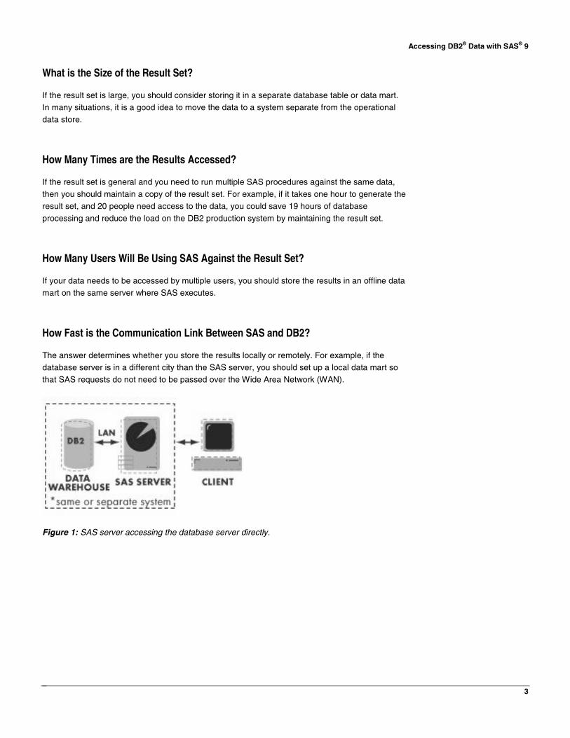
How Fast is the Communication Link Between SAS and DB2?

The answer determines whether you store the results locally or remotely. For example, if the database server is in a different city than the SAS server, you should set up a local data mart so that SAS requests do not need to be passed over the Wide Area Network (WAN).

Figure 1: SAS server accessing the database server directly.


4

Figure 2: SAS server accessing a data mart.

Usage Scenarios

The following usage scenarios provide examples of applying the list of questions to developing a data processing model. These scenarios assume that the query generating the result takes many

hours to complete and is resource-intensive.

Scenario 1

You are the only user accessing the data. You need to access the database once, and you can reuse the result set to complete your analysis.

In this case, you should create a local copy of the result set and use it for your analysis.

Scenario 2

Ten to twenty SAS users are accessing the data and querying it multiple times using different

procedures.

In this case, you should save the result set of the initial query in a data mart so that all SAS users

can access it.

Scenario 3

Your SAS users require input from multiple data sources.

In many SAS environments, data is collected by one or more database administrators and sent to the SAS user for analysis. You can streamline this process in two ways. You can retrieve the data directly from the source. SAS allows you to execute procedures against multiple data sources in a

single step, and SAS collects all the data for you. Alternatively, you can use IBM’s Information Integration technology to collect data. An Information Integration server provides a single view to multiple data sources as if they all existed on a single DB2 server. This single view allows the


5

database administrator to provide a secure, central data access point for SAS users. Both methods simplify the collection of data from multiple sources.

Figure 3: Gateway accessing multiple data sources.

Scenario 4

You use SAS to analyze the status of your just-in-time inventory system.

In this case, the data that you retrieve needs to be up-to-date. Accessing an operational DB2 database is the answer. To enable this type of evaluation, you should consider using the DB2

Materialized Query Table (MQT) or the DB2 8.1 Multidimensional Clustering (MDC) feature to improve query performance.

Using the DB2 MQT and/or MDC feature allow(s) you to organize your data for more efficient access by organizing or pre-computing the data required by your SAS application. MQT supplies aggregations and joining of data. MDC allows you to organize the storage of a table along multiple

dimensions. In either case, SAS does not need special knowledge of the data to use these features. MDC is applied on the source table itself, defined when the table is created. MQT is a separate table containing the aggregated results.

For example, if you are analyzing data by region, you can use an MQT to pre-compute values by region. In this case, when your SAS application requests the information, much of the

computation is done. The following code example shows a MQT that contains information aggregated by state.


6

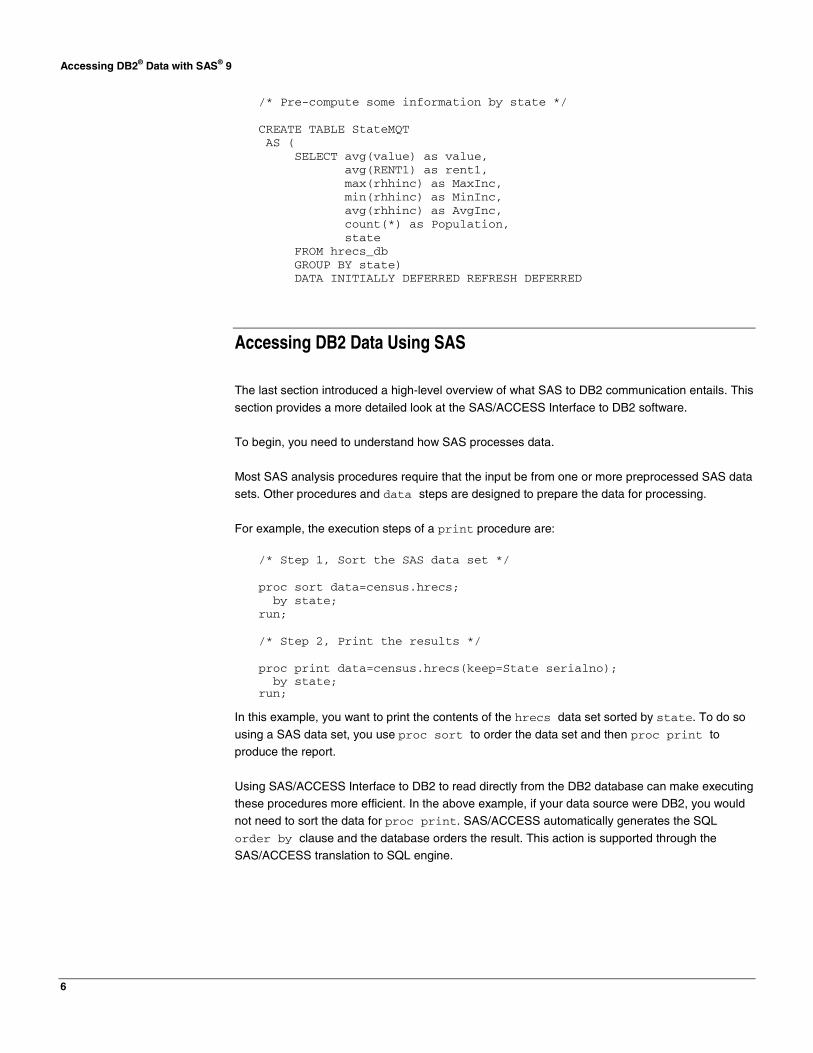
/* Pre-compute some information by state */ CREATE TABLE StateMQT AS ( SELECT avg(value) as value, avg(RENT1) as rent1, max(rhhinc) as MaxInc, min(rhhinc) as MinInc, avg(rhhinc) as AvgInc, count(*) as Population, state FROM hrecs_db GROUP BY state) DATA INITIALLY DEFERRED REFRESH DEFERRED

Accessing DB2 Data Using SAS

The last section introduced a high-level overview of what SAS to DB2 communication entails. This

section provides a more detailed look at the SAS/ACCESS Interface to DB2 software.

To begin, you need to understand how SAS processes data.

Most SAS analysis procedures require that the input be from one or more preprocessed SAS data sets. Other procedures and data steps are designed to prepare the data for processing.

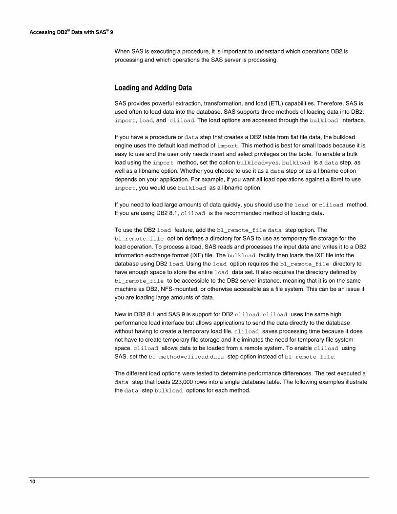
For example, the execution steps of a print procedure are:

/* Step 1, Sort the SAS data set */ proc sort data=census.hrecs; by state; run; /* Step 2, Print the results */ proc print data=census.hrecs(keep=State serialno); by state; run;

In this example, you want to print the contents of the hrecs data set sorted by state. To do so

using a SAS data set, you use proc sort to order the data set and then proc print to produce the report.

Using SAS/ACCESS Interface to DB2 to read directly from the DB2 database can make executing these procedures more efficient. In the above example, if your data source were DB2, you would not need to sort the data for proc print. SAS/ACCESS automatically generates the SQL

order by clause and the database orders the result. This action is supported through the SAS/ACCESS translation to SQL engine.


7

When migrating your SAS code so that you can use SAS/ACCESS Interface to DB2, make sure that you remove procedures that do not apply to the database (proc sort for example). In the

example above, if you run proc sort against the database, it will exit with an error indicating that the database table does not work in replace mode. This error does not impact performance. If, on the other hand, proc sort sends the data to a separate database table, SAS/ACCESS

will execute a select with order by statement and insert the results. Database tables are not ordered, so this would be an unnecessary processing step and would impact performance.

Database Access from SAS

There are two ways to connect to your DB2 database from SAS. You can connect using the

libname engine, or you can connect directly to the database using the connect statement in the SQL procedure.

When connecting to the database using the libname engine, SAS automatically translates SAS data access application code to SQL. Translation to SQL means that SAS/ACCESS processes the SAS application code and then generates the appropriate SQL to access the database.

When connecting directly to the database using the connect statement, you can use explicit SQL pass-through. Explicit SQL pass-through is a mechanism that allows you to pass unaltered

SQL directly to the database server. Explicit SQL pass-through is useful for adding database-only operations to your SAS application and is accessible using the SQL procedure (proc sql).

Most SAS procedures and data steps use the SAS/ACCESS SQL translation engine. Following is an example of SQL translation for the print procedure in the preceding example. When the same proc print procedure is executed using SAS/ACCESS against a DB2 database, the

request is translated into SQL for processing by DB2.

/* SQL generated or proc print */ select “state”,”serialno” from hrecs order by state;

This is the SQL generated for the proc print statement. As mentioned earlier, proc sort would not be necessary in this case.

When Would You Use SAS/ACCESS Translation to SQL?

You should use the SAS/ACCESS translation to SQL when:

• You want to use SAS data access functionality (for example, threaded reads).

• You are joining data from multiple data sources.

• The application needs to be portable to different relational databases.

• The procedure or data step requires it (for example, proc freq, proc summary).

Performance Tip:

Porting

If you are migrating code from

using a SAS data set to using

DB2, make sure you remove

unnecessary procedures like

proc sort. Even though they are

not necessary they will execute

and take time to process.


8

When Would You Use Explicit SQL Pass-Through?

Explicit SQL pass-through should be used when:

• DB2 database processing steps are executed from a SAS application.*

• You want to use DB2-specific SQL.

Using the SAS/ACCESS libname Engine

The libname engine is used by SAS 9 to access data libraries (a data source). By way of the libname engine, SAS uses the relational database library to access a DB2 database.

The SAS libname engine allows you to easily modify applications to use different data sources. You can modify a SAS statement that uses a SAS data set to use a table in your DB2 database instead by simply changing the libname definition. For example, the following is a script that

accesses a SAS data set named mylib.data1 to generate frequency statistics.

/* Define the directory /sas/mydata as a SAS library */ libname mylib data “/sas/mydata”; /* Run frequency statistics against the data1 data set */ proc freq data=mylib.data1; where state=’01’; table state tenure yrbuilt yrmoved msapmsa; run;

To run frequency statistics against the data1 table in your DB2 database, change the libname statement to access the data1 table instead of the SAS data set:

libname mylib db=DB2 user=me using=password;

Now, when this procedure is executed, SAS/ACCESS generates the proper SQL to retrieve the data from the database.

select "state", "tenure", "yrbuilt", "yrmoved", "msapmsa" from data1 where state=‘01’;

Using the libname engine is the easiest way to access DB2 database tables from your SAS application because SAS generates the appropriate SQL for you. The next example uses a data step to demonstrate how the SQL translation engine works.

* SAS does not need to manipulate the data, and all work is done in the DB2 database server.

Coding Tip:

Accessing long or case-

sensitive table names

If you need to access data from

tables that are not in all

uppercase, set the following

libname option:

preserve_tab_names=yes

This setting enables you to pass

case-sensitive or long table

names to the database and is

important when accessing data

using the SAS GUI tools. If you

do not see the table names

using the SAS Explorer, try

setting this option.


9

In the following example, the data step reads and filters the data from the source table source1 and writes the results to the database table results1. The results1 table contains all the

housing records for state ID 01.

libname census db=DB2 user=me using=password; data census.results1; set census.source1; where state=‘01’; run;

SAS begins by opening a connection to the database to retrieve metadata and create the results1 table. The connection is used to read all the rows for state=’01’ from source1.

SAS opens a second connection to write the rows to the newly created results1 table. If this were a multi-tier configuration, the data would travel over the network twice. First, it would travel from the database server to the SAS server. Then, it would travel from the SAS server back to the

database server. SAS processes the data in this manner to support moving data between various sources. This type of connection allows you to read data from one database server and to write the results to a different database. Because a single data source is used and SAS does not need

to process the data, this operation can be made more efficient.

To make this operation more efficient, you can use the explicit SQL pass-through facility of the

sql procedure. To make this statement explicit, create a sql procedure with the necessary SQL statements. Connect to the database using the connect statement, and wrap the SQL using the execute statement. For example:

proc sql; connect to db2 (database=census); execute(create table results1 like source1) as db2; execute(insert into results1 select * from source1 where state=‘01’) by db2; disconnect from db2; quit;

On the test system, the original data step executed in 33 seconds, and the explicit proc sql executed in 15 seconds. Changing to explicit SQL improved the performance of the operation by 64 percent. Because all the work can be done by the DB2 database, explicit SQL is the most

efficient way to process the statement.

Explicit Pass-Through Versus SQL Translation

In the preceding example, explicit SQL should be used instead of SQL translation (also known as implicit SQL) because an implicit proc sql statement is processed using a similar SQL

translation engine as a data step.

If the same statement is passed as implicit SQL, SAS breaks the statement into separate select

and insert statements. The performance gain was realized with explicit SQL because all the processing was handled by the database server.

Performance Tip:

Coding

If SAS does not need to process

the data, let the database do as

much work as possible. Explicit

SQL is the best way to force the

database to process data.


10

When SAS is executing a procedure, it is important to understand which operations DB2 is processing and which operations the SAS server is processing.

Loading and Adding Data

SAS provides powerful extraction, transformation, and load (ETL) capabilities. Therefore, SAS is used often to load data into the database. SAS supports three methods of loading data into DB2: import, load, and cliload. The load options are accessed through the bulkload interface.

If you have a procedure or data step that creates a DB2 table from flat file data, the bulkload engine uses the default load method of import. This method is best for small loads because it is

easy to use and the user only needs insert and select privileges on the table. To enable a bulk load using the import method, set the option bulkload=yes. bulkload is a data step, as well as a libname option. Whether you choose to use it as a data step or as a libname option

depends on your application. For example, if you want all load operations against a libref to use import, you would use bulkload as a libname option.

If you need to load large amounts of data quickly, you should use the load or cliload method. If you are using DB2 8.1, cliload is the recommended method of loading data.

To use the DB2 load feature, add the bl_remote_file data step option. The bl_remote_file option defines a directory for SAS to use as temporary file storage for the load operation. To process a load, SAS reads and processes the input data and writes it to a DB2

information exchange format (IXF) file. The bulkload facility then loads the IXF file into the database using DB2 load. Using the load option requires the bl_remote_file directory to have enough space to store the entire load data set. It also requires the directory defined by

bl_remote_file to be accessible to the DB2 server instance, meaning that it is on the same machine as DB2, NFS-mounted, or otherwise accessible as a file system. This can be an issue if you are loading large amounts of data.

New in DB2 8.1 and SAS 9 is support for DB2 cliload. cliload uses the same high performance load interface but allows applications to send the data directly to the database

without having to create a temporary load file. cliload saves processing time because it does not have to create temporary file storage and it eliminates the need for temporary file system space. cliload allows data to be loaded from a remote system. To enable cliload using

SAS, set the bl_method=cliload data step option instead of bl_remote_file.

The different load options were tested to determine performance differences. The test executed a

data step that loads 223,000 rows into a single database table. The following examples illustrate the data step bulkload options for each method.


11

/* Method: import */ data HSET(bulkload=yes); <…data step processing…> run; /* Method: load */ data HSET(bulkload=yes bl_remote_file=”/tmp”); <…data step processing…> run; /* Method: cliload */ data HSET(bulkload=yes bl_method=cliload); <…data step processing…> run;

Load Method Time in seconds

import 76.69

load 55.93

cliload 49.04

The table shows that by using cliload, there is a 36 percent performance gain over the import method. All load options require that the table does not exist before the load.

Creating Tables

SAS/ACCESS can automatically create DB2 tables for you in the same way that SAS data sets are created. When SAS automatically creates a database table using default options, it can use three DB2 data types — double, varchar, and timestamp. If you would like the database

table created with a specific data type, use the dbtype= data set option, or define variable formats in your application.

In the following example, the SERIALNO and PUMA columns are set to the DB2 data types bigint and char(25) when the table is created.

data census.results1 (dbtype=(SERIALNO=’bigint’PUMA=’char(25)’)); set census.source1; where state=‘01’; run;

In addition, SAS creates different data types based on SAS variable formats. In the following, SAS determines what type of numeric column to create based on the size and precision as defined in the variable format.

SAS Format DB2 Data Type

format col1 4.0 smallint

format col1 7.0 int

format col1 5.2 Decimal

The previous table shows an example of numeric conversions. SAS supports many other

format-to-column type conversions.


12

To set other DB2-specific table creation options, you should use the create_table_opts libname option. create_table_opts appends whatever you include to the end of the create

table statement. The following is an example that creates a table containing all rows from source1 where the state is 01.

data census.results1; set census.source1; where state=‘01’; run;

If this table is being created in a partitioned database, you could specify the partitioning key by adding the dbcreate_table_opts option and then specifying a portioning scheme.

data census.results1 (dbcreate_table_opts=’partitioning key(serialno)’; set census.source1; where state=‘01’; run;

When SAS generates the create table statement, the partitioning clause is appended

to the end of the statement.

create table results1 (SERIALNO double, PUMA varchar(20), [column list…]) partitioning key(serialno);

When using SAS to create database tables, you can use the dbcreate_table_opts and

dbtype options to customize the tables to ease administration and improve performance.

Retrieving the Data into SAS

When reading from a DB2 database with SAS/ACCESS, you can control access to partitioned tables, use multiple SAS threads to scan the database, and utilize CLI multi-row fetch capabilities.

SAS 9 and DB2 8.1 have great improvements in the read performance of SAS applications. Threaded read is one of these new SAS 9 features. Threaded read allows SAS to extract data from DB2 in parallel, which means faster processing of a large or partitioned database. In

DB2 8.1, multi-row fetch has been improved, increasing read performance up to 45 percent over single-row fetch.

What Are the Performance Impacts of These Operations?

There are three different SAS tuning parameters that can improve the speed of data transfer from

DB2 to SAS: readbuff, dbsliceparm, and dbslice. These parameters correspond to the DB2 functions multi-row fetch, mod(), and custom where clause predicates respectively.


13

SAS Function DB2 Function

readbuff multi-row fetch

dbsliceparm mod()

dbslice custom where clause predicates

To examine the performance differences between these functions, frequency statistics were run

against a database table on the test system. To generate frequency information, SAS retrieves all the rows in the table.

The first test was run using the default read options: single-row fetch and non-threaded read.

libname census db2 db=census user=db2inst1 using=password; proc freq data=census.hrecs_db table state tenure yrbuilt yrmoved msapmsa; run;

This test ran in 72.02 seconds.

readbuff

Using the default options, SAS executes a single thread that reads one row at a time through the DB2 CLI interface. Transfer speed can be improved by sending multiple rows in each request using multi-row fetch. SAS/ACCESS supports the DB2 multi-row fetch feature via the libname

readbuff option. readbuff=100 was added to the libname statement, and the test was run again on the test system.

libname census db2 db=census user=db2inst1 using=password readbuff=100;

This test ran in 43.33 seconds, which is a 40 percent performance improvement over a single row fetch.

This procedure was tested with other values of readbuff. The testing indicated that the optimal value for this procedure is between 200 and 250, which allowed the query to run in 40.97 seconds. With readbuff set to 200, the new multi-threaded read options were tested using the

same procedure.

Figure 4: Results of readbuff testing.


14

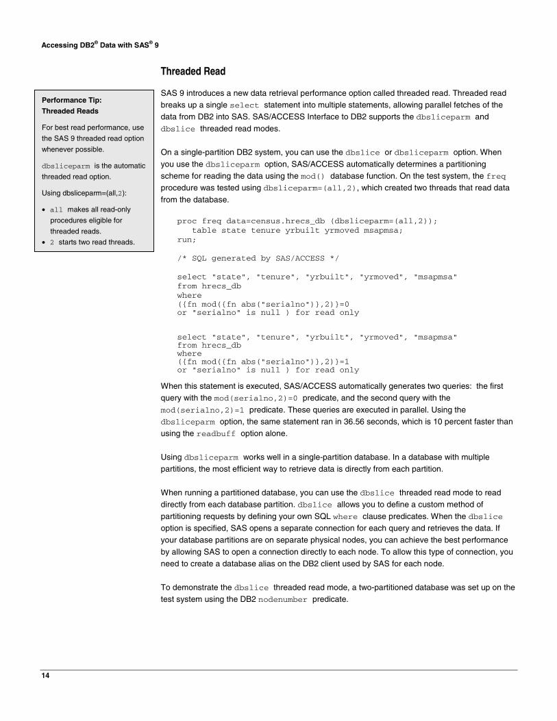
Threaded Read

SAS 9 introduces a new data retrieval performance option called threaded read. Threaded read breaks up a single select statement into multiple statements, allowing parallel fetches of the data from DB2 into SAS. SAS/ACCESS Interface to DB2 supports the dbsliceparm and

dbslice threaded read modes.

On a single-partition DB2 system, you can use the dbslice or dbsliceparm option. When

you use the dbsliceparm option, SAS/ACCESS automatically determines a partitioning scheme for reading the data using the mod() database function. On the test system, the freq procedure was tested using dbsliceparm=(all,2), which created two threads that read data

from the database.

proc freq data=census.hrecs_db (dbsliceparm=(all,2)); table state tenure yrbuilt yrmoved msapmsa; run; /* SQL generated by SAS/ACCESS */ select "state", "tenure", "yrbuilt", "yrmoved", "msapmsa" from hrecs_db where ({fn mod({fn abs("serialno")},2)}=0 or "serialno" is null ) for read only select "state", "tenure", "yrbuilt", "yrmoved", "msapmsa" from hrecs_db where ({fn mod({fn abs("serialno")},2)}=1 or "serialno" is null ) for read only

When this statement is executed, SAS/ACCESS automatically generates two queries: the first query with the mod(serialno,2)=0 predicate, and the second query with the

mod(serialno,2)=1 predicate. These queries are executed in parallel. Using the dbsliceparm option, the same statement ran in 36.56 seconds, which is 10 percent faster than using the readbuff option alone.

Using dbsliceparm works well in a single-partition database. In a database with multiple partitions, the most efficient way to retrieve data is directly from each partition.

When running a partitioned database, you can use the dbslice threaded read mode to read directly from each database partition. dbslice allows you to define a custom method of

partitioning requests by defining your own SQL where clause predicates. When the dbslice option is specified, SAS opens a separate connection for each query and retrieves the data. If your database partitions are on separate physical nodes, you can achieve the best performance

by allowing SAS to open a connection directly to each node. To allow this type of connection, you need to create a database alias on the DB2 client used by SAS for each node.

To demonstrate the dbslice threaded read mode, a two-partitioned database was set up on the test system using the DB2 nodenumber predicate.

Performance Tip:

Threaded Reads

For best read performance, use

the SAS 9 threaded read option

whenever possible.

dbsliceparm is the automatic

threaded read option.

Using dbsliceparm=(all,2):

• all makes all read-only

procedures eligible for

threaded reads.

• 2 starts two read threads.


15

/* Catalog a node */ catalog tcpip node dbnode1 remote myserver server 70000 /* Catalog a database */ catalog database dbname at node dbnode1

Using a two-partition DB2 database on the test server, the dbsliceparm option was replaced with dbslice syntax in the freq procedure script. Because the test database consisted of multiple partitions on a single system, only a single node was cataloged. The freq procedure

was executed using the dbslice option, along with the nodenumber syntax.

proc freq data=census.hrecs_db (dbslice=("nodenumber(serialno)=0" "nodenumber(serialno)=1")); table state tenure yrbuilt yrmoved msapmsa; run;

To execute the request, SAS opened two connections to the database server and executed the

SQL necessary to retrieve data from each partition.

/* SQL generated by SAS/ACCESS */ select "state", "tenure", "yrbuilt", "yrmoved", "msapmsa" from hrecs_db where nodenumber(serialno)=0 for read only select "state", "tenure", "yrbuilt", "yrmoved", "msapmsa" from hrecs_db where nodenumber(serialno)=1 for read only

The query ran in 35.13 seconds, which is 14 percent faster than using the readbuff option alone.

Threaded read options improve data extraction performance. As the database size or number of partitions increases, threaded read options could help even more.

Not all operations take advantage of threaded reads. A statement does not qualify for threaded reads if:

• A by statement is used.

• The obs option is specified.

• The firstobs option is specified.

• The key/dbkey= option is specified.

• There is no valid input column for the mod() function (effects dbsliceparm).

• All valid columns for the mod() function are listed in the where clause (effects dbsliceparm).

• The nothreads option is specified.

• The value of dbsliceparm option is set to none.

Performance Note:

readbuff Results

For consistency, performance

using readbuff with no

threaded read options was

tested in a multiple partition

configuration. The results of the

readbuff test were the same

as the single node, making them

comparable.

Performance Tip:

Coding

It is best to limit the amount of

data transferred between DB2

and SAS. If you need only a few

columns for your analysis, list

the columns you need from the

source table. In the example to

the left, changing:

set census.source1;

to:

set census.source1

(keep=state puma);

tells SAS to only retrieve the

columns needed.


16

If your statement does not qualify for threaded reads and you attempt to enable it, then the SAS log will contain an error, for example:

Threading is disabled due to the ORDER BY clause or the FIRSTOBS/OBS option …

Putting Data into Your DB2 Database

Read performance is most important when using SAS to extract data from DB2. However, it is also important to tune applications that insert rows to the database. This section examines two ways to improve the performance of inserting data: dbcommit and insertbuff.

dbcommit

The dbcommit parameter sets the number of rows that are inserted into the database between transaction commits. To insert one row into a database table, there are many operations that take place behind the scenes to complete the transaction.

For example, the DB2 database transaction log records all modifications to the database to ensure data integrity. During an insert, multiple records are recorded to the database transaction

log. The first record is the insert itself, followed by the commit record that tells the database that the transaction is complete. For example, if you were to insert 1000 rows, with each row being its own transaction, the entire procedure would require 2000 transaction log records (1000 insert

records plus 1000 commit records). In contrast, if all of these inserts were in a single transaction, there would be 1001 transaction log records (1000 insert plus 1 commit). There is a considerable difference in the amount of work required to insert the same 1000 rows, depending on how the

transaction is structured.

If you are doing an insert, one option would be to set dbcommit to the total number of rows you

need to insert. Keep in mind, however, that with any performance tuning, there are tradeoffs.

For example, if you were to insert one million rows in a single transaction, you would need a lock

to be held for each row. As the number of locks required increases, the overhead for lock management increases. Therefore, you should adjust the value of dbcommit to be large enough to limit commit processing, but not so large that you encounter long transaction issues (locking,

running out of log space, etc.). To test insert performance, a data step is used that processes the hrecs table and creates a new hrecs_temp table containing all the rows where state=‘01’.

libname census db2 db=census user=db2inst1 using=password; data census.hrecs_temp (dbcommit=10000); set census.hrecs; where state='01'; run;


17

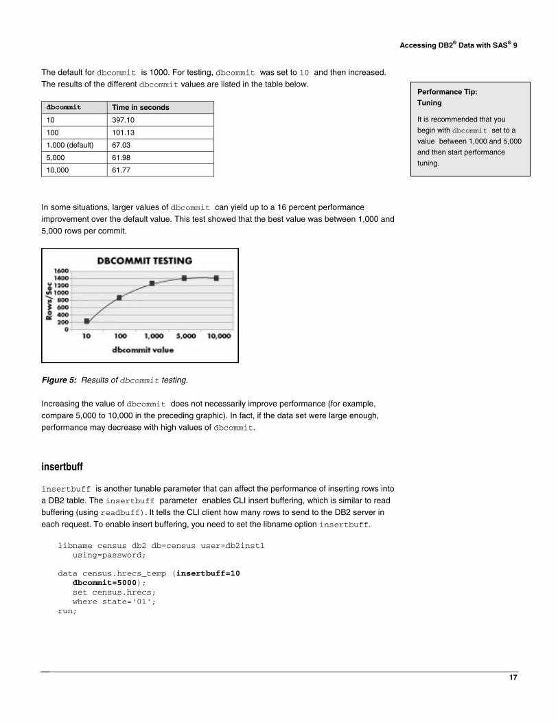
The default for dbcommit is 1000. For testing, dbcommit was set to 10 and then increased. The results of the different dbcommit values are listed in the table below.

dbcommit Time in seconds

10 397.10

100 101.13

1,000 (default) 67.03

5,000 61.98

10,000 61.77

In some situations, larger values of dbcommit can yield up to a 16 percent performance improvement over the default value. This test showed that the best value was between 1,000 and 5,000 rows per commit.

Figure 5: Results of dbcommit testing.

Increasing the value of dbcommit does not necessarily improve performance (for example, compare 5,000 to 10,000 in the preceding graphic). In fact, if the data set were large enough, performance may decrease with high values of dbcommit.

insertbuff

insertbuff is another tunable parameter that can affect the performance of inserting rows into a DB2 table. The insertbuff parameter enables CLI insert buffering, which is similar to read buffering (using readbuff). It tells the CLI client how many rows to send to the DB2 server in

each request. To enable insert buffering, you need to set the libname option insertbuff.

libname census db2 db=census user=db2inst1 using=password; data census.hrecs_temp (insertbuff=10 dbcommit=5000); set census.hrecs; where state='01'; run;

Performance Tip:

Tuning

It is recommended that you

begin with dbcommit set to a

value between 1,000 and 5,000

and then start performance

tuning.


18

The value of insertbuff can be an integer ranging from 1 to 2,147,483,648. Different values of insertbuff were tested to see what impact it would have on the preceding data step. The

results are listed in the table below.

insertbuff Time in seconds

1 61.77

5 60.64

10 60.22

25 60.36

50 60.36

100 60.86

Increasing the value of insertbuff from 1 to 25 improved the performance only 2.7 percent

over the tuned dbcommit environment. Increasing the value over 25 did not have a significant impact on performance. However, performance can vary from one set up to another, even when you use the exact same parameter values. So, to show possible differences, the same test was

run with SAS and DB2 running on separate servers using a TCP/IP connection instead of a local shared memory connection. Results are shown in the table below.

insertbuff TCP/IP Time in seconds

1 150.75

5 109.05

10 104.52

25 99.35

50 98.23

100 98.11

In this environment, increasing the value of insertbuff from 1 to 25 had a significant impact on performance, which improved 51 percent over the default.

These results show that when you are running in a local (shared memory) configuration, insertbuff has little impact on performance, and you may want to tune dbcommit for optimal performance. On the other hand, when you are connecting from a separate server, insertbuff

can have a significant impact on performance.

The best values for insertbuff are about 10 times smaller than the best values for readbuff.

You should keep this in mind when you are tuning your system.

More on the SQL Procedure

The SQL procedure (proc sql) is a powerful way to access DB2 data from your SAS application. The SQL procedure enables access to multiple data sources in a single statement

and allows the application to be portable across different relational databases.

Performance Tip:

proc append

Use proc append to add data

to an existing table. This

procedure uses the same insert

process as the previous data

step, so the same tuning rules

apply.


19

In addition, proc sql is well suited to data manipulation and processing, similar to a data step. Moving more processing into the SQL procedure and then pushing it into DB2 can save data

step processing time later.

When a proc sql statement is executed, SAS determines what portions of the request can be

pushed to the database and what is to be processed in SAS. SQL translation is more powerful in proc sql than in other procedures. In addition to passing down where clause processing, SQL translation in proc sql can pass join and function operations to DB2. For example, if your SQL

includes a multi-table join, SAS can pass join processing to the database server. Pushing join operations to the database can improve performance when working with large data sets.

Joining Data Sets (Tables)

SAS can push join processing to the database if all the tables are in the same library or if the

librefs involved meet certain conditions. For SAS/ACCESS to push join processing across multiple librefs to the database, all libraries must have the same:

• user ID.

• Password.

• Update_Isolation_Level (if specified).

• Read_Isolation_Level (if specified).

• Qualifier.

• Data source.

In addition, prompt must not be specified.

Joining across multiple librefs can be helpful if you need to join tables from different schemas

because each libref is associated with one schema.

Joining tables using proc sql is not the same as a merge data step statement. When using

proc sql, the default is an inner join, whereas a SAS data set merge is equivalent to a left outer join. This can cause different results to be generated, depending on your join condition.

Function Pushdown

If the database supports the function that you request, SAS can pass the processing of that

function to the DB2 server. To enable the most functions to be pushed to DB2, set the sql_functions=all libname option.

Coding Tip:

Join versus Data Set Merge

A SAS data set merge is

equivalent to a left outer join in

proc sql.


20

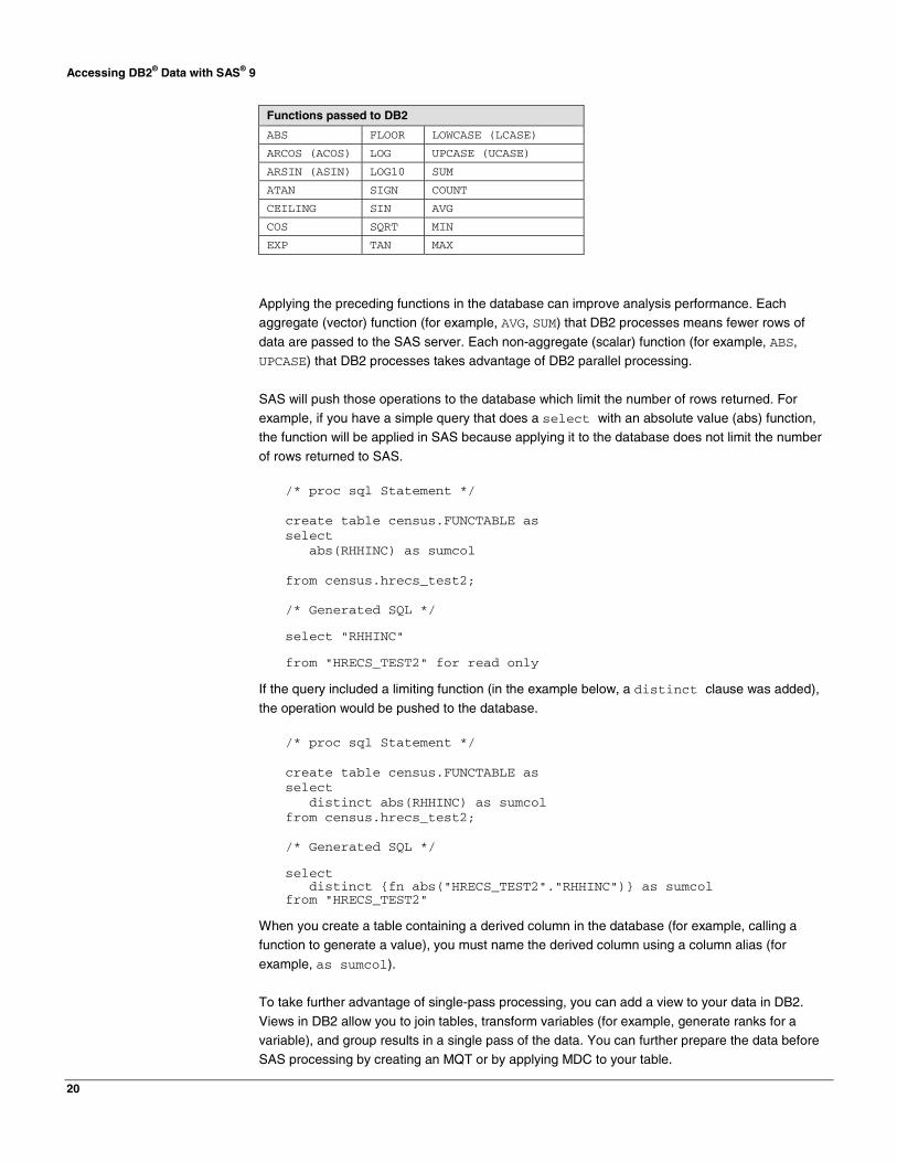
Functions passed to DB2

ABS FLOOR LOWCASE (LCASE) ARCOS (ACOS) LOG UPCASE (UCASE) ARSIN (ASIN) LOG10 SUM ATAN SIGN COUNT CEILING SIN AVG COS SQRT MIN EXP TAN MAX

Applying the preceding functions in the database can improve analysis performance. Each aggregate (vector) function (for example, AVG, SUM) that DB2 processes means fewer rows of

data are passed to the SAS server. Each non-aggregate (scalar) function (for example, ABS, UPCASE) that DB2 processes takes advantage of DB2 parallel processing.

SAS will push those operations to the database which limit the number of rows returned. For example, if you have a simple query that does a select with an absolute value (abs) function, the function will be applied in SAS because applying it to the database does not limit the number

of rows returned to SAS.

/* proc sql Statement */ create table census.FUNCTABLE as select abs(RHHINC) as sumcol from census.hrecs_test2; /* Generated SQL */ select "RHHINC" from "HRECS_TEST2" for read only

If the query included a limiting function (in the example below, a distinct clause was added),

the operation would be pushed to the database.

/* proc sql Statement */ create table census.FUNCTABLE as select distinct abs(RHHINC) as sumcol from census.hrecs_test2; /* Generated SQL */ select distinct {fn abs("HRECS_TEST2"."RHHINC")} as sumcol from "HRECS_TEST2"

When you create a table containing a derived column in the database (for example, calling a function to generate a value), you must name the derived column using a column alias (for

example, as sumcol).

To take further advantage of single-pass processing, you can add a view to your data in DB2.

Views in DB2 allow you to join tables, transform variables (for example, generate ranks for a variable), and group results in a single pass of the data. You can further prepare the data before SAS processing by creating an MQT or by applying MDC to your table.


21

The Database Administrator’s Corner

How Does SAS Use My Database?

To a DB2 database administrator, SAS is another consumer of database resources. This section explains the way SAS connects to the database and how it uses other database resources.

Included are some debugging tips for SAS applications in a SAS/ACCESS Interface to DB2 environment.

Connections

Each SAS client opens multiple connections to the database server. When a SAS session is

started, a single data connection is opened to the database. This connection is used for most communication from SAS to DB2. If the SAS application requires metadata from DB2 catalogs (by executing proc datasets, for example), a second utility connection is created. This utility

connection allows SAS to collect the information without interfering with the original data connection. In addition, it allows the utility operations to exist in a separate transactional context.

By default, the two connections remain active until the SAS session is completed or the libname reference or database connection (opened using the connect statement) is explicitly closed. Other connections may be opened automatically during a SAS session. These connections are

closed when the operation for which they were opened is completed. For example, if you read from one table and write to a new table, SAS opens two connections: the original connection to retrieve the data and the second connection to write the data into the new table. In this example,

the connection used to write the data will be closed when the data step is completed.

You can control how connections are managed in SAS/ACCESS using the

connection=libname option. The default connection mode is sharedread, which means all read operations in a single SAS session use a common connection for reading data. If you need to limit the total number of connections opened to the database, you should use the shared

option. The shared mode uses one connection per SAS session for all data operations except the utility connection. This mode limits each SAS client to two connections: one data connection (read and write) and one utility connection. By default, the utility connection stays around for the

duration of the SAS session.

There are many different connection modes, including sharedread, unique, shared,

globalread, and global. The sharedread, unique, and shared options were used to test the performance implications of sharing connections.

The append procedure was used to measure the impact of different connection options. Connection testing was done with SAS and DB2 running on separate systems because the impact of the connection type is more apparent when using TCP/IP instead of local shared

memory.

The first test executed a proc append, which reads from one table and appends the results to

another table in the same database. Using proc append allows testing in a mixed read/write environment.

Note:

Threaded Reads

Threaded read operations do

not abide by the connection

settings. So, even if

connection is set to the

default of sharedread, a single

operation, for example, using

dbsliceparm will open

multiple connections to the

database.


22

libname census db2 db=census user=user1 using=password connection=unique; proc append BASE=census.append1 data=census.hrecsca; run;

This test executed proc append in three different connection modes: sharedread (default), shared, and unique. The sharedread mode opens one connection for all read operations and

opens separate connections for each write operation. The shared mode opens one connection for each SAS session for read and write operations. The unique mode opens a separate connection for each read and write operation. The table below shows the results of the test.

Connection Mode Time in seconds

sharedread 38.35

shared 130.90

unique 39.24

Results showed that the shared read mode is 241 percent slower than the other two

connection options. Before using the shared mode, you should test the possible impact on your workload. For example, if your environment is more read-oriented, using shared may not have a large impact. In a read/write environment, if your goal is to use fewer connections, you should

schedule the jobs to limit concurrent access instead of sharing connections.

Resource Consumption

Database administrators are always interested in what impact an application has on a database. SAS workloads can vary greatly depending on the environment. The following are tips on how to

start evaluating your situation:

• Each SAS user is the equivalent of a single database Decision Support (DS) user. So, you

should tune SAS as if you were tuning for an equivalent number of generic DS users.

• Tune to the workload. Like any other DS application, understanding the customer

requirements can help you improve system performance. For example, if there is a demand for quarterly or monthly data, using an MDC table for the data may be appropriate.

• SAS is a DS application. If you need data from an operational data store, consider the impact on other applications. To offload some of the workload, you should consider creating a data mart to provide data to your SAS customers.

• In most environments, the SAS server is located on a separate system from the database. Business analysis often requires many rows of data to be retrieved from the database. Plan

to provide the fastest network connection possible between systems to provide the greatest throughput.

• As with any workload, keep your database statistics up-to-date using runstats. This option enables the optimizer to generate the best possible access plan.

Here are some general guidelines for optimizing performance:


23

• Try to pass as much where clause and join processing as you can to DB2.

• Return only the rows and columns you need. Whenever possible, do not use a select * … from your SAS application. For example, provide a list of the necessary columns, using keep=(var1, var2…). To limit the number of rows returned, include any appropriate filters

in the where clause.

• Provide MDC tables or MQT where appropriate to provide precompiled results for faster

access to data.

• Use SAS threaded read (dbsliceparm, dbslice) and multi-row fetch (readbuff)

operations whenever possible.

• When loading data with SAS, use the cliload method.

Debugging

The sastrace option allows you to see what SQL commands SAS is passing to the database. For example, the syntax to trace the SQL calls that SAS/ACCESS SQL makes to DB2 is as follows:

options sastrace “,,,d” sastraceloc=saslog;

Applying a “d” in the fourth column of the sastrace option tells SAS to report SQL sent to the database. For example, the following data step:

data census.hrecs_temp (keep=year rectype serialno state); keep year rectype serialno state; set census.hrecs_db; where state=1; run;

is logged as the following (the SQL commands are highlighted):

TRACE: Using EXTENDED FETCH for file HRECS_DB on connection 0 476 1372784097 rtmdoit 0 DATASTEP

TRACE: SQL stmt prepared on statement 0, connection 0 is: SELECT * FROM HRECS_DB FOR READ ONLY 477 1372784097 rtmdoit 0 DATASTEP

TRACE: DESCRIBE on statement 0, connection 0. 478 1372784097 rtmdoit 0 DATASTEP

622 data census.hrecs_temp (keep=YEAR RECTYPE SERIALNO STATE); 623 keep YEAR RECTYPE SERIALNO STATE; 624 set census.hrecs_db; 625 where state=1; 626 run; TRACE: Using FETCH for file HRECS_TEMP on connection 1 479 1372784097 rtmdoit 0 DATASTEP

TRACE: Successful connection made, connection id 2 480 1372784097 rtmdoit 0 DATASTEP


24

TRACE: Database/data source: census 481 1372784098 rtmdoit 0 DATASTEP

TRACE: USER=DB2INST1, PASS=XXXXXXX 482 1372784098 rtmdoit 0 DATASTEP

TRACE: AUTOCOMMIT is NO for connection 2 483 1372784098 rtmdoit 0 DATASTEP

TRACE: Using FETCH for file HRECS_TEMP on connection 2 484 1372784098 rtmdoit 0 DATASTEP

NOTE: SAS variable labels, formats, and lengths are not written to DBMS tables.

TRACE: SQL stmt execute on connection 2: CREATE TABLE HRECS_TEMP (YEAR DATE,RECTYPE VARCHAR(1),SERIALNO NUMERIC(11,0),STATE NUMERIC(11,0)) 485 1372784098 rtmdoit 0 DATASTEP

TRACE: COMMIT performed on connection 2. 486 1372784098 rtmdoit 0 DATASTEP

TRACE: SQL stmt prepared on statement 0, connection 0 is: SELECT "YEAR", "RECTYPE", "SERIALNO", "SAMPLE", "DIVISION", "STATE", "PUMA", "AMORTG2", "AMRTAMT2", "ACNDOFEE", "AMOBLHME" FROM HRECS_DB WHERE ("STATE" = 1 ) FOR READ ONLY 487 1372784098 rtmdoit 0 DATASTEP

TRACE: Open cursor from statement 0 on connection 0 488 1372784098 rtmdoit 0 DATASTEP

TRACE: Preparing SQL statement: INSERT INTO HRECS_TEMP (YEAR,RECTYPE,SERIALNO,STATE) VALUES ( ? , ? , ? , ? ) 489 1372784099 rtmdoit 0 DATASTEP


NOTE: There were 86100 observations read from the data set

CENSUS.HRECS_DB.

WHERE state=1;

TRACE: Close cursor from statement 0 on connection 0 576 1372784184 rtmdoit 0 DATASTEP


NOTE: The data set CENSUS.HRECS_TEMP has 86100 observations and 4 variables.



The sastrace option displays the processing details of the SAS script. The log includes the

exact SQL commands that are submitted to the database. The preceding code example executes a data step that SAS translates into the following four SQL statements:

select * from hrecs_db; create table hrecs_temp (year date,rectype varchar(1),serialno numeric(11,0),state numeric(11,0)); select "year", "rectype", "serialno", "sample", "division", "state", "puma", "amortg2", "amrtamt2", "acndofee", "amoblhme" from hrecs_db where ("state"=1);

Hint:

To find SQL information, search

the log for SQL.


25

insert into hrecs_temp (year,rectype,serialno,state) values ( ? , ? , ? , ? );

By using DB2, you can see what SAS/ACCESS is requesting on the database by enabling CLI trace. This feature is useful for debugging SAS/ACCESS interaction with DB2.

There are two ways to enable CLI trace: by entering the DB2 Command Line Processor (CLP) command update cli cfg or by editing the sqllib/cfg/db2cli.ini file. To use the

command, enter:

db2 update cli cfg for section COMMON using TraceFileName /tmp/mytracefile

then:

db2 update cli config for COMMON using trace 1

To edit the db2cli.ini file, directly add trace and TraceFileName in the COMMON section

[COMMON] trace=1 TraceFileName=/tmp/mytracefile TraceFlush=1

When you enable CLI tracing, DB2 begins tracing all CLI statements executed on the server. DB2

continues to trace CLI statements until you disable CLI tracing by setting trace to 0. Keep in mind that if the server is busy, you could collect huge amounts of output. It is best to run CLI tracing on a test server running a single SAS session if possible.

The SAS log and DB2 log (the DB2 log is located in sqllib/db2dump/sqdb2diag.log) are useful places to look for information when you are troubleshooting.

What is Ahead for SAS and DB2?

Working together, SAS and IBM deliver solutions that meet your most complex business intelligence needs. SAS 9 and DB2 8.1 provide expanded functionality and performance via SAS bulkload and threaded read, and via DB2 multi-row fetch and cliload performance. For the

future, SAS and IBM remain committed to providing a leading combination of analysis solutions with greater scalability and performance.

World Headquartersand SAS AmericasSAS Campus DriveCary, NC 27513 USATel: (919) 677 8000Fax: (919) 677 4444U.S. & Canada sales: (800) 727 0025

SAS InternationalPO Box 10 53 40 Neuenheimer Landstr. 28-30D-69043 Heidelberg, GermanyTel: (49) 6221 4160 Fax: (49) 6221 474850

www.sas.com

SAS and all other SAS Institute Inc. product or service names are registered trademarks or trademarks of SAS Institute Inc. in the USA and other countries. ® indicates USA registration. Other brand and product names are trademarks of their respective companies. Copyright © 2002, SAS Institute Inc. All rights reserved. 09/03

accessing db2 data with sas 9 · pdf fileaccessing db2 ® data with sas 9 1 introduction...

Documents