access to microfinance by rural women: implications for

Research in Applied Economics ISSN 1948-5433

2013, Vol. 5, No. 2

www.macrothink.org/rae 19

Access to Microfinance by Rural Women: Implications

for Poverty Reduction in Rural Households in Ghana

Samuel Kobina Annim1 & Samuel Erasmus Alnaa2,*

1Department of Economics, University of Cape Coast, University Post Office, Cape Coast, Ghana

2Department of Accountancy, Bolgatanga Polytechnic, P.O. Box 767, Bolgatanga, Ghana

*Correponding author: Department of Accountancy, Bolgatanga Polytechnic, P.O. Box 767, Bolgatanga, Ghana Tel: 233-242-803-715 E-mail: [email protected]

Received: December 30, 2012 Accepted: February 20, 2013 Published: May 27, 2013

doi:10.5296/rae.v5i2.2974 URL: http://dx.doi.org/10.5296/rae.v5i2.2974

Abstract

In view of the recent evidence that the impact of microfinance is being overstated, this study assesses the causal link between receiving credit from a microfinance institution and poverty reduction among rural households in the Upper East Region of Ghana. Using consumption expenditure as the outcome variable, we test the hypothesis that receiving credit has a poverty reducing effect. Treatment effect estimation technique is used to examine data on 250 beneficiaries and 250 non-beneficiaries from five Districts in the Region. Although the method of study is based on a quasi-experimental approach, the process of selecting the beneficiary and non-beneficiary sample cautiously made an attempt to minimize the potential problems that will arise from contamination, spill-over effects and programme and self-exclusion selection biases. The results support the hypothesis that microfinance has 0.12% poverty reducing effect. Premised on this, we conclude that even in very poor areas microfinance is capable of reducing poverty. Therefore microfinance investment is recommended to broaden the scale and scope of beneficiaries reached and improve delivery strategies to suite context specific characteristics.

JEL Classification: C1, D13, D14, G21

Keywords: access; microfinance; poverty reduction; rural women; treatment effects and Ghana


2013, Vol. 5, No. 2


1. Introduction

The revolution in the Microfinance (MF) industry has created a development paradigm shift. This paradigm shift favours the use of MF as an important ingredient in improving the welfare of the poor particularly in developing countries. This has come about as a result of: (1) the call by The 1997 Microfinance Summit for the mobilization of US$20 billion over a 10-year period to support microfinance; (2) The proclamation of 2005 by the United Nations as the “Year of Micro-credit”; and (3) the ultimate award of a Nobel Peace Prize to a universally acclaimed founder of modern microfinance, Prof. Muhamad Yunus and the Grameen Bank which he founded in 1970. These milestones in the history of MF, can be said to have partially propelled the boom in the MF industry.

It has been estimated that at least 400 million poor and low-income people are not being served by MF programmes (IFAD, 2004). Usually, the poor has no access to loans from the banking system, because they cannot put up acceptable collateral and/or because the costs for banks in screening and monitoring the activities of the poor, and enforcing their contracts, are too high to make lending to this group profitable. This situation has serious negative impact on poor households struggling to reduce poverty, vulnerability, and attain food security. Access to credit enables poor people to smooth consumption in times of income variability and also engage in microenterprises which lead to value creation and ultimately move the poor out of poverty.

Microfinance has been found as an important tool for fighting poverty particularly in the developing countries and a plethora of studies attest to this (Remenyi & Quinones, 2000; Morduch & Haley, 2002; Khandker, 2005; Gobezie & Garber, 2007; Imai & Azam, 2010; Imai, Arun & Annim, 2010; Ghalib, Malki & Imai, 2011). Though various studies have pointed to this fact, some of the findings have been contested and have pointed to the contrary (e.g. Banerjee et al., 2009; Karlan & Zinman, 2009; Feigenberg et al. 2010).

Poverty in Ghana is said to be a disproportionately rural phenomenon. The report of the Ghana Living Standards Survey round five (GLSS5) indicates that eighty-six percent of the total population who live below the poverty line in Ghana, reside in rural areas. The report further indicates that 50% of these rural poor live in rural savannah (Ghana Statistical Service, 2007). In the light of this, MF interventions over the years were imperative. The financial sector reforms in Ghana, particularly, the promulgation of PNDC Law 328 in 1991 to allow the establishment of different categories of non-bank financial institutions, including savings and loans companies, and credit unions, gave an impetus to the MF industry in Ghana to further grow. This was to meet the ever increasing financial needs of poor households who are usually unreached and underserved by the traditional financial institutions. In sub-Saharan Africa (SSA), as at 2007, Ghana was ranked the highest recipient (about US$186m) of development partner’s donor funding into microfinance (CGAP, 2008). Thus in the spirit of poverty alleviation most of the MFIs in Ghana particularly Financial Non-governmental Organizations targeted rural households. This was to enable the beneficiaries engage in income generating activities so as to improve upon their livelihoods.

In a similar vein, the Upper East Region (UER) which according to the GLSS5, is the second


2013, Vol. 5, No. 2


poorest Region in the country with about 70% of the population living below the poverty line (GSS, 2008), received MF services targeting rural poor women. Most of these women engaged in agro-processing activities such as rice milling, shea-butter extraction, malt making and so forth. Thus financial services from MFIs were meant to help these women boost their output, increase their earnings and ultimately improve upon their socio-economic welfare.

Despite the fact that the UER has received much support in the areas of MF, it is still not clear if this has been able to reduce the poverty level of beneficiaries and their households. Studies in the areas of MF that seek to establish the link between MF and the welfare outcomes are inconclusive as reports on the impact of MF on poverty reduction are conflicting. In this regard, further exploration of the impact of MF under varying assumptions and in different context is important. In the light of this, we test the hypothesis that receiving credit has a poverty reducing effect

2. Microfinance Impact Studies

Microfinance is hailed by many as an important tool for poverty alleviation. This is so for a number of reasons. Microfinance allows poor people to protect, diversify, and increase their sources of income. Microfinance enables poor people to overcome their liquidity constraints and undertake some investment in a micro-enterprise or in improved farm technology and inputs, thereby leading to increased incomes or agricultural production (Okurut, Banga & Mukungu, 2004). Furthermore credit helps the poor people to smooth out their consumption patterns during the lean periods of the year (Binswanger & Khandker, 1995). This is believed to be the most promising path out of poverty and hunger.

Gobezie & Garber (2007) using matured clients and incoming clients as the treatment group and control group respectively in a study of microfinance clients in the Amhara region of northern Ethiopia, found improved household diet, resulting from higher household income, this was measured in food condition, quality and quantity of food, among others. Results from the Impact survey showed that clients were eating more frequently and increasing the quantity of food eaten. The study specifically indicated that, relatively higher proportion (83%) of mature clients were said not to have any problem of food security in the household during the last 12 months, compared to only about 73% of new clients. Though the performance of mature clients was quite impressive, it was not clear if the issue of randomization in terms of participation in the programme was done. This creates sample selection bias with its attendant problems of over estimation of the programme impact. Also the issue of endogeneity was not tested. These two problems have the effect of bias estimation of the project effects. Failure to account for this therefore implies that the benefits of the programme alluded to can not be wholly attributed to the programme participation as some confounding variables may simply be responsible for the impacts found. On the other hand the use of matured and incoming clients creates another problem of the control group and participating group having pre-existing differences which may explain why one group chose to participate in the MF programme earlier. These pre-existing differences if not


2013, Vol. 5, No. 2


effectively dealt with then the project impact can not be entirely attributed to MF.

In a study in Bangladesh, Imai & Azam (2010) used household panel data covering rounds from 1997 to 2005. The study employed the treatment effects model and propensity score matching (PSM) for the participants and non-participants of microfinance programmes. With the treatment effect model the study found that simple household access to general loans from MFIs did not increase per capita household income significantly but household access to loans for productive purposes from MFIs significantly increased per capita household income. The study therefore emphasizes the importance of the purpose and monitoring of how clients use the loans in a bid to increase household income and for that matter decreasing household poverty. The study further found that, with the application of treatment effects and PSM to each cross-sectional component of the panel data, the poverty reducing effect of MFI on poverty was significantly reduced over the years.

In a related study by Imai, Arun & Annim (2010) in India found that loans for productive purposes were more important for poverty reduction in rural than in urban areas. However in urban areas, simple access to MFIs had larger average poverty-reducing effects than the access to loans from MFIs for productive purposes. Again using Propensity Score Matching to control for sample selection bias in a study in Pakistan, Ghalib, Malki & Imai (2011) confirmed that microfinance programmes had positive impact on the welfare of beneficiary household in terms of expenditure on healthcare or clothing, monthly household income, and certain dwelling characteristics such as water supply and quality of roofing and walls.

Even though scores of studies have shown positive impacts of microfinance on poverty, other studies point to the contrary (Morduch, 1999; Kiiru, 2008). Kiiru has noted that microfinance can not be expected as a “magic bullet” against poverty (Kiiru, 2008). These controversies have therefore led to the criticism of microfinance as a catalyst of poverty reduction. Again Kiiru & Mburu (2006) have argued that microfinance can not improve welfare unless there is effective demand for goods and services, which ensures that the products of micro-entrepreneurs are consumed. The most-noted studies on the impact of microcredit on households according to Roodman & Morduch (2009) are based on a survey fielded in Bangladesh in the 1990s. They noted that the contradictions among them have produced lasting controversy and confusion.

3. Method and Data

The study employed a quasi-experimental survey. Thus the data for the study was obtained from both beneficiaries (treatment group) and non-beneficiaries (control group) of MFI loans in 2011 through a random survey of 500 women engaged in agro-processing in the Upper East Region of Ghana of whom 250 were beneficiaries of microfinance while 250 were non-beneficiaries. Questionnaires were administered to the randomly selected respondents in a face-to-face interview. The questions included in the interview relate to access to microfinance, initial savings, consumption expenditure on basic needs, the number of business activities the woman engages in at the moment, the location of the business, and


2013, Vol. 5, No. 2


several other socio-demographic characteristics.

3.1 Sampling Technique and Attribution

The study’s sampling procedure for reaching the treatment and control groups was done in a manner to minimise biases that characterise non-experimental impact research. The rationale was to mimic a randomized control trial. The following highlights some of the strategies employed to minimize spill-over effects, confounding problems, and contamination and selection biases. First, to deal with spill-over effects, the control and treatment groups were selected from different communities. The choice of communities was preceded by a focused group discussion in all the communities in the district. The rationale was to ascertain information on the extent of interaction among communities and gain insight on issues such as the similarity between communities and interventions related to poverty and finance that have been received by communities. Placement bias has been associated with selecting treatment and control groups from different communities. In this study, this is less of a concern as MFIs are situated mainly in the District capitals. Thus, the likelihood of the control group indirectly receiving some benefits from the treatment group in view of their access to credit is minimized (Duvendack et al., 2011).

Second, selection bias; as indicated by Duvendack et al. (2011) and Hulme(n.d.) occurs when there is no randomization in the assignment of subjects under study into either treatment or control group. This therefore creates a pre-existing difference between the treatment and the control groups. When this happens it leads to an inconsistent or bias estimate of the impact of the programme intervention. Thus to minimize the problem of selection bias, the study selected respondents with similar characteristics, such engagement in agro-processing business, respondents resident in rural communities and other household characteristics. The entrepreneurial drive and ability which is an invisible attribute was therefore effectively taken care of as well as other economic, physical and social environment.

Thirdly, Contamination; this is said to occur when there is communication about the experiment between groups of participants. That is subjects under study are aware of the study and communicate among themselves about the study. There are three possible outcomes of contamination. Some participants’ performance may worsen because they resent being in a less desirable condition; also participants in a less desirable condition may boost their performance so they don’t look bad; and diffusion of treatments: control participants learn about a treatment and apply it to themselves. This issue of contamination was taken care of in the study by interviewing individual respondents in each group in their respective homes, so that no one knows of the other in the study. Again the control and treatment groups were selected from different communities (Duvendack et al., 2011; Hulme, n.d.).

3.2 Model Specification

Given the fact that there is potential selection bias and issues of endogeneity which have come about because MFIs choose communities in which they want to operate (to lend) deliberately (known as endogenous programme placement), and also because individuals themselves choose to borrow or not borrow (known as endogenous programme participation),


2013, Vol. 5, No. 2


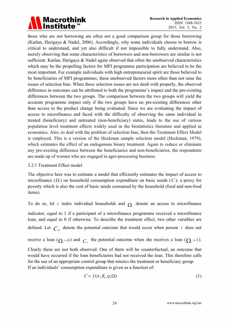
those who are not borrowing are often not a good comparison group for those borrowing (Karlan, Harigaya & Nadel, 2006). Accordingly, why some individuals choose to borrow is critical to understand, and yet also difficult if not impossible to fully understand. Also, merely observing that some characteristics of borrowers and non-borrowers are similar is not sufficient. Karlan, Harigaya & Nadel again observed that often the unobserved characteristics which may be the propelling factors for MFI programme participation are believed to be the most important. For example individuals with high entrepreneurial spirit are those believed to be beneficiaries of MFI programmes, these unobserved factors more often than not raise the issues of selection bias. When these selection issues are not dealt with properly, the observed difference in outcomes can be attributed to both the programme’s impact and the pre-existing differences between the two groups. The comparison between the two groups will yield the accurate programme impact only if the two groups have no pre-existing differences other than access to the product change being evaluated. Since we are evaluating the impact of access to microfinance and faced with the difficulty of observing the same individual in treated (beneficiary) and untreated (non-beneficiary) states, leads to the use of various population level treatment effects widely used in the biostatistics literature and applied in economics. Also, to deal with the problem of selection bias, then the Treatment Effect Model is employed. This is a version of the Heckman sample selection model (Heckman, 1979), which estimates the effect of an endogenous binary treatment. Again to reduce or eliminate any pre-existing difference between the beneficiaries and non-beneficiaries, the respondents are made up of women who are engaged in agro-processing business.

3.2.1 Treatment Effect model

The objective here was to estimate a model that efficiently estimates the impact of access to microfinance ( ) on household consumption expenditure on basic needs (C ); a proxy for poverty which is also the cost of basic needs consumed by the household (food and non-food items).

To do so, let i index individual households and i denote an access to microfinance

indicator, equal to 1 if a participant of a microfinance programme received a microfinance loan, and equal to 0 if otherwise. To describe the treatment effect, two other variables are

defined. Let 0iC denote the potential outcome that would occur when person i does not

receive a loan ( 0i ) and

1iC the potential outcome when she receives a loan ( 1i ).

Clearly these are not both observed. One of them will be counterfactual, an outcome that would have occurred if the loan beneficiaries had not received the loan. This therefore calls for the use of an appropriate control group that mimics the treatment or beneficiary group. If an individuals’ consumption expenditure is given as a function of:

1( , , , )C f R (1)


2013, Vol. 5, No. 2


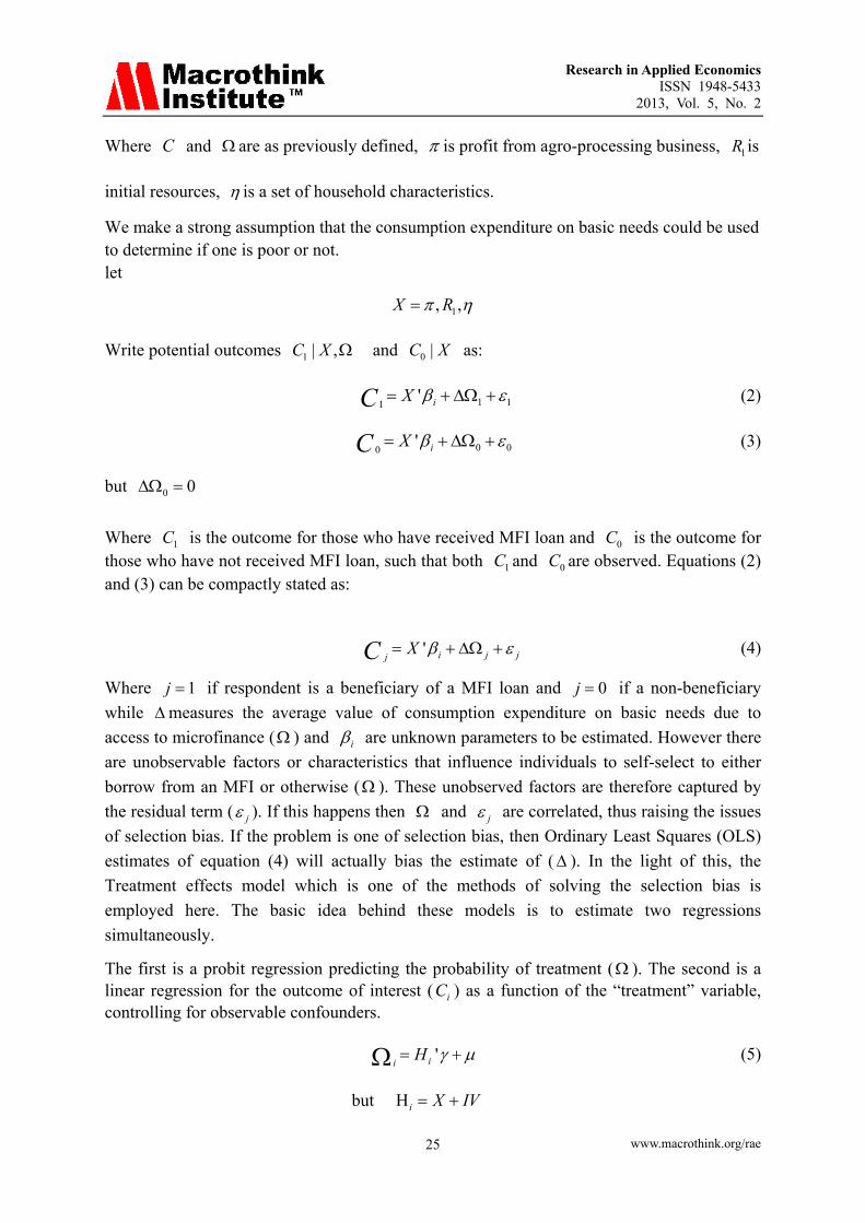
Where C and are as previously defined, is profit from agro-processing business, 1R is

initial resources, is a set of household characteristics.

We make a strong assumption that the consumption expenditure on basic needs could be used to determine if one is poor or not. let

1, ,X R

Write potential outcomes 1 | ,C X and 0 |C X as:

1 11' iXC (2)

0 00' iXC (3)

but 0 0

Where 1C is the outcome for those who have received MFI loan and 0C is the outcome for those who have not received MFI loan, such that both 1C and 0C are observed. Equations (2) and (3) can be compactly stated as:

' i j jjXC (4)

Where 1j if respondent is a beneficiary of a MFI loan and 0j if a non-beneficiary

while measures the average value of consumption expenditure on basic needs due to

access to microfinance ( ) and i are unknown parameters to be estimated. However there

are unobservable factors or characteristics that influence individuals to self-select to either

borrow from an MFI or otherwise ( ). These unobserved factors are therefore captured by

the residual term ( j ). If this happens then and j are correlated, thus raising the issues

of selection bias. If the problem is one of selection bias, then Ordinary Least Squares (OLS)

estimates of equation (4) will actually bias the estimate of ( ). In the light of this, the

Treatment effects model which is one of the methods of solving the selection bias is

employed here. The basic idea behind these models is to estimate two regressions

simultaneously.

The first is a probit regression predicting the probability of treatment ( ). The second is a linear regression for the outcome of interest ( iC ) as a function of the “treatment” variable, controlling for observable confounders.

'iiH (5)

but Hi X IV


2013, Vol. 5, No. 2


That is, iH which are the variables determining access to MF contain all the elements in X

plus at least an additional element ( IV ) not in X . This satisfies the exclusion restriction

requirement.

But corr ( , ) 0

It is assumed that the error terms ( and ) are jointly normally distributed and a maximum

likelihood methods of estimation was used. Because corr ( , ) 0 then appropriate

Instrumental Variable(s) (IV) must be found to solve the problem. In which case IV must be

correlated with i but not correlated with iC .

Thus the expected consumption expenditure for those who have received MFIs loans is given by the joint density bivariate normally distributed variables and of the formula:

( ' )[ | 1] ' [ | 1] '

( ' )i

i i i i ii

hE C X E X

h

(6)

Where, is the standard normal density function and is the standard normal cumulative distribution function. The ratio of and is called the inverse Mill’s ratio (IMR) (sometimes also called 'selection hazard' particularly in the treatment effect model) or control functions and it takes account of possible selection bias. When the coefficient of IMR is positive there are unobserved variables that both increase the probability of selection and a higher than average score on the dependent variable. When the coefficient of IMR is negative there are unobserved variables increasing the probability of selection and the probability of a lower than average score on the dependent variable. The expected consumption expenditure for those who have access without participation in microfinance programme (have not received MFIs loans) is given as:

( ' )

[ | 0] ' [ | 0] '1 ( ' )

ii i i i i

i

hE C X E X

h

(7)

The expected effect of poverty reduction as a result of access to microfinance programme can be calculated as:

( ' )

[ | 1] [ | 0]( ' )[1 ( ' )]

ii i i i

i i

hE C E C

h h

(8)

If is positive (negative), then the coefficient estimate of employing the method of OLS will be biased upwards (downwards), but the sample selection term (inverse mills ratio) will


2013, Vol. 5, No. 2


correct for this (Imai, Arun and Annim, 2010). The sign and significance of the estimate of

( ) shows if selection bias exists.

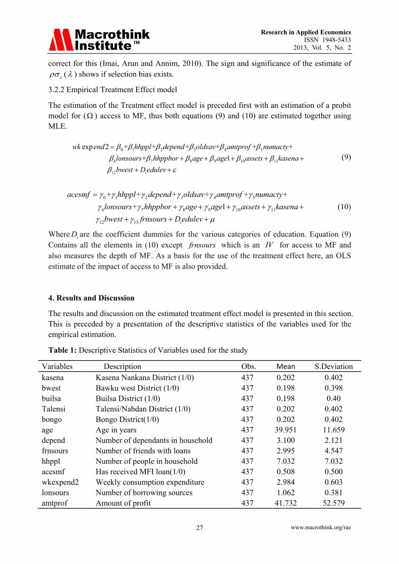
3.2.2 Empirical Treatment Effect model

The estimation of the Treatment effect model is preceded first with an estimation of a probit model for ( ) access to MF, thus both equations (9) and (10) are estimated together using MLE.

0 1 2 3 4 5

6 7 8 9 10 11

12

exp 2 + + + + + +

+ 1

i

wk end hhppl depend oldsav amtprof numacty

lonsours hhppbor age age assets kasena

bwest D edulev

(9)

0 1 2 3 4 5

6 7 8 9 10 11

12 13

+ + + + + +

+ 1

i

acesmf hhppl depend oldsav amtprof numacty

lonsours hhppbor age age assets kasena

bwest frnsours D edulev

(10)

Where iD are the coefficient dummies for the various categories of education. Equation (9) Contains all the elements in (10) except frnsours which is an IV for access to MF and also measures the depth of MF. As a basis for the use of the treatment effect here, an OLS estimate of the impact of access to MF is also provided.

4. Results and Discussion

The results and discussion on the estimated treatment effect model is presented in this section. This is preceded by a presentation of the descriptive statistics of the variables used for the empirical estimation.

Table 1: Descriptive Statistics of Variables used for the study

Variables Description Obs. Mean S.Deviation

kasena Kasena Nankana District (1/0) 437 0.202 0.402 bwest Bawku west District (1/0) 437 0.198 0.398 builsa Builsa District (1/0) 437 0.198 0.40 Talensi Talensi/Nabdan District (1/0) 437 0.202 0.402 bongo Bongo District(1/0) 437 0.202 0.402 age Age in years 437 39.951 11.659 depend Number of dependants in household 437 3.100 2.121 frnsours Number of friends with loans 437 2.995 4.547 hhppl Number of people in household 437 7.032 7.032 acesmf Has received MFI loan(1/0) 437 0.508 0.500 wkexpend2 Weekly consumption expenditure 437 2.984 0.603 lonsours Number of borrowing sources 437 1.062 0.381 amtprof Amount of profit 437 41.732 52.579


2013, Vol. 5, No. 2


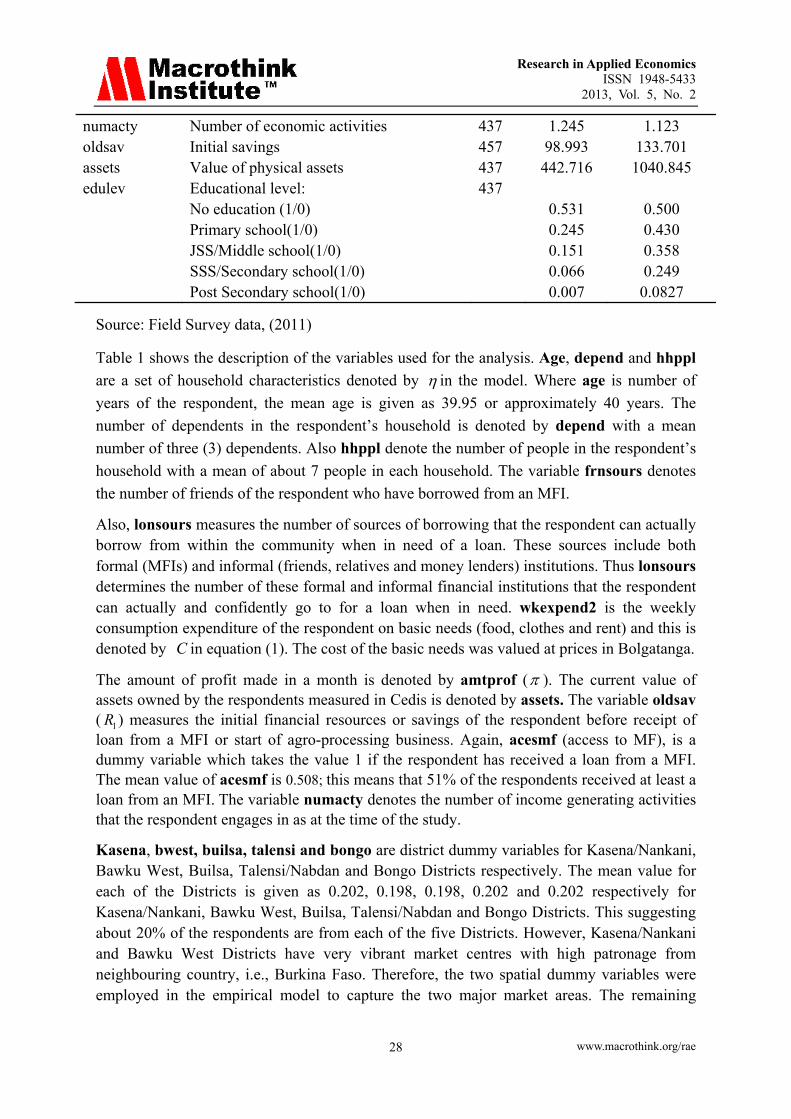
numacty Number of economic activities 437 1.245 1.123 oldsav Initial savings 457 98.993 133.701 assets Value of physical assets 437 442.716 1040.845 edulev Educational level: 437

No education (1/0) 0.531 0.500 Primary school(1/0) 0.245 0.430 JSS/Middle school(1/0) 0.151 0.358 SSS/Secondary school(1/0) 0.066 0.249 Post Secondary school(1/0) 0.007 0.0827

Source: Field Survey data, (2011)

Table 1 shows the description of the variables used for the analysis. Age, depend and hhppl

are a set of household characteristics denoted by in the model. Where age is number of

years of the respondent, the mean age is given as 39.95 or approximately 40 years. The

number of dependents in the respondent’s household is denoted by depend with a mean

number of three (3) dependents. Also hhppl denote the number of people in the respondent’s

household with a mean of about 7 people in each household. The variable frnsours denotes

the number of friends of the respondent who have borrowed from an MFI.

Also, lonsours measures the number of sources of borrowing that the respondent can actually borrow from within the community when in need of a loan. These sources include both formal (MFIs) and informal (friends, relatives and money lenders) institutions. Thus lonsours determines the number of these formal and informal financial institutions that the respondent can actually and confidently go to for a loan when in need. wkexpend2 is the weekly consumption expenditure of the respondent on basic needs (food, clothes and rent) and this is denoted by C in equation (1). The cost of the basic needs was valued at prices in Bolgatanga.

The amount of profit made in a month is denoted by amtprof ( ). The current value of assets owned by the respondents measured in Cedis is denoted by assets. The variable oldsav ( 1R ) measures the initial financial resources or savings of the respondent before receipt of loan from a MFI or start of agro-processing business. Again, acesmf (access to MF), is a dummy variable which takes the value 1 if the respondent has received a loan from a MFI. The mean value of acesmf is 0.508; this means that 51% of the respondents received at least a loan from an MFI. The variable numacty denotes the number of income generating activities that the respondent engages in as at the time of the study.

Kasena, bwest, builsa, talensi and bongo are district dummy variables for Kasena/Nankani, Bawku West, Builsa, Talensi/Nabdan and Bongo Districts respectively. The mean value for each of the Districts is given as 0.202, 0.198, 0.198, 0.202 and 0.202 respectively for Kasena/Nankani, Bawku West, Builsa, Talensi/Nabdan and Bongo Districts. This suggesting about 20% of the respondents are from each of the five Districts. However, Kasena/Nankani and Bawku West Districts have very vibrant market centres with high patronage from neighbouring country, i.e., Burkina Faso. Therefore, the two spatial dummy variables were employed in the empirical model to capture the two major market areas. The remaining


2013, Vol. 5, No. 2


Districts; Builsa, Talensi/Nabdan and Bongo Districts which do not have vibrant market centres were used as the reference categories.

Also, the variable edulev is a categorical variable; it measures the highest educational level of the respondent. The mean of each level (category) of education shows the proportion (percentage) of the respondents in that category. Thus out of this variable, 53.1% have no education; 24.5% have Primary school education; 15.1% have JSS/Middle school education; 6.6% have Senior Secondary School (SSS)/ secondary school education while 0.7% have post secondary school education. Respondents with no education are used as the reference category.

Table 2 shows the results of OLS estimate of equation (4). The dependent variable is lwkexpend2 which is the natural log of wkexpend2. Thus lwkexpend2 measures the percentage of weekly expenditure on basic needs due to the independent variable(s). From the Table kasena, bwest, depend, oldsav, amtprof, age, Primary, JSS/Middle, Post secondary, numacty and acesmf all are statistically different from zero and each of them has a positive relationship with the percentage of weekly expenditure (proxy for poverty).

The coefficient of acesmf (0.2122) implies that beneficiaries of MFIs loans on the average spend 21.2% weekly on basic needs more than non-beneficiaries of MFIs loan. However, due to the issues of selection bias and endogeneity OLS estimate of the coefficient of acesmf (0.2122) is bias and for that matter does not provide an accurate measure of the impact of access to MF. In the light of this, the treatment effect model is estimated which controls for sample selection bias.

Tables 3a and 3b show the results of the treatment effect model, which have been simultaneously estimated using the access to MF (acesmf) and the outcome (weekly consumption expenditure (wkexpend2)). Table 3a shows the results of access to MF equation with acesmf as the dependent variable. While Table 3b shows the results of the weekly expenditure equation: with the natural log of weekly expenditure on basic needs, a proxy for poverty (lwkexpend2) as the dependent variable.

Table 2: Results of OLS estimation of impact of access to MF (dependent variable: weekly consumption expenditure)

Variables Coefficient Robust Std. error P-Value

Kasena Nankana District (1/0) 0.341*** 0.072 0.000 Bawku west District (1/0) 0.548*** 0.063 0.000 Age in years 0.052*** 0.016 0.001 Age-squared -0.001*** 0.000 0.001 Number of dependants in household 0.033** 0.014 0.017 Number of people in household -0.006 0.008 0.477 Has received MFI loan(1/0) 0.212*** 0.050 0.000 Number of borrowing sources -0.009 0.051 0.855 Amount of profit 0.002*** 0.001 0.003 No. of income generating activities 0.045** 0.019 0.019


2013, Vol. 5, No. 2


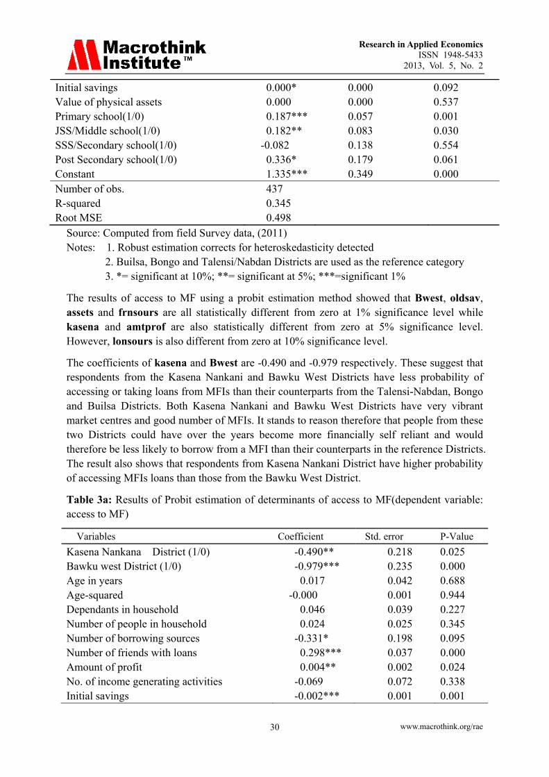
Initial savings 0.000* 0.000 0.092 Value of physical assets 0.000 0.000 0.537 Primary school(1/0) 0.187*** 0.057 0.001 JSS/Middle school(1/0) 0.182** 0.083 0.030 SSS/Secondary school(1/0) -0.082 0.138 0.554 Post Secondary school(1/0) 0.336* 0.179 0.061 Constant 1.335*** 0.349 0.000 Number of obs. 437 R-squared 0.345 Root MSE 0.498

Source: Computed from field Survey data, (2011) Notes: 1. Robust estimation corrects for heteroskedasticity detected 2. Builsa, Bongo and Talensi/Nabdan Districts are used as the reference category 3. *= significant at 10%; **= significant at 5%; ***=significant 1%

The results of access to MF using a probit estimation method showed that Bwest, oldsav, assets and frnsours are all statistically different from zero at 1% significance level while kasena and amtprof are also statistically different from zero at 5% significance level. However, lonsours is also different from zero at 10% significance level.

The coefficients of kasena and Bwest are -0.490 and -0.979 respectively. These suggest that respondents from the Kasena Nankani and Bawku West Districts have less probability of accessing or taking loans from MFIs than their counterparts from the Talensi-Nabdan, Bongo and Builsa Districts. Both Kasena Nankani and Bawku West Districts have very vibrant market centres and good number of MFIs. It stands to reason therefore that people from these two Districts could have over the years become more financially self reliant and would therefore be less likely to borrow from a MFI than their counterparts in the reference Districts. The result also shows that respondents from Kasena Nankani District have higher probability of accessing MFIs loans than those from the Bawku West District.

Table 3a: Results of Probit estimation of determinants of access to MF(dependent variable: access to MF)

Variables Coefficient Std. error P-Value

Kasena Nankana District (1/0) -0.490** 0.218 0.025 Bawku west District (1/0) -0.979*** 0.235 0.000 Age in years 0.017 0.042 0.688 Age-squared -0.000 0.001 0.944 Dependants in household 0.046 0.039 0.227 Number of people in household 0.024 0.025 0.345 Number of borrowing sources -0.331* 0.198 0.095 Number of friends with loans 0.298*** 0.037 0.000 Amount of profit 0.004** 0.002 0.024 No. of income generating activities -0.069 0.072 0.338 Initial savings -0.002*** 0.001 0.001


2013, Vol. 5, No. 2


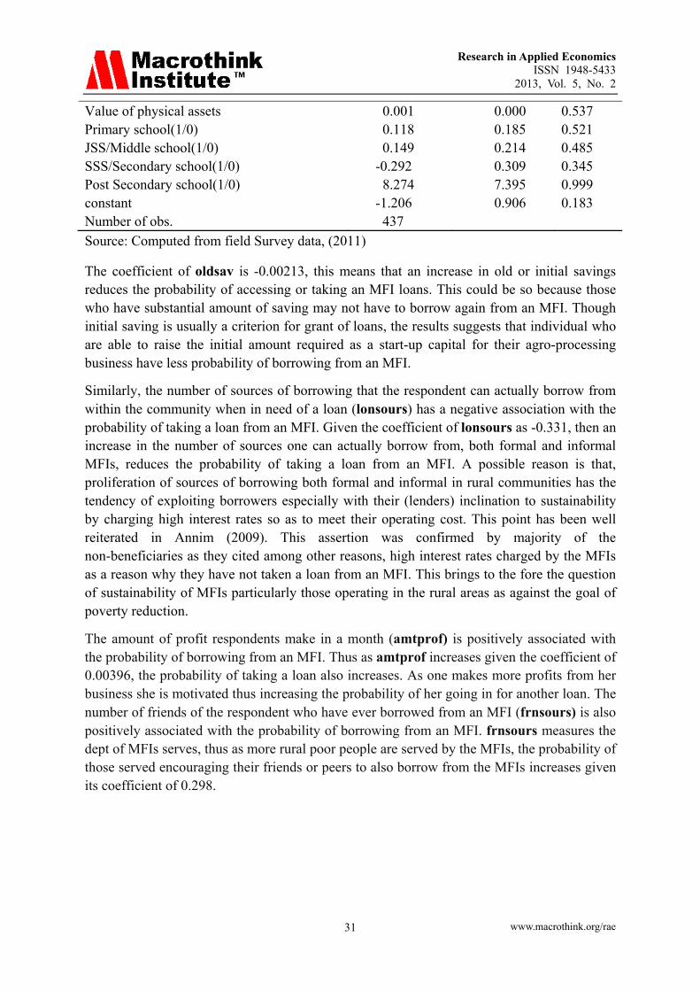
Value of physical assets 0.001 0.000 0.537 Primary school(1/0) 0.118 0.185 0.521 JSS/Middle school(1/0) 0.149 0.214 0.485 SSS/Secondary school(1/0) -0.292 0.309 0.345 Post Secondary school(1/0) 8.274 7.395 0.999 constant -1.206 0.906 0.183 Number of obs. 437

Source: Computed from field Survey data, (2011)

The coefficient of oldsav is -0.00213, this means that an increase in old or initial savings reduces the probability of accessing or taking an MFI loans. This could be so because those who have substantial amount of saving may not have to borrow again from an MFI. Though initial saving is usually a criterion for grant of loans, the results suggests that individual who are able to raise the initial amount required as a start-up capital for their agro-processing business have less probability of borrowing from an MFI.

Similarly, the number of sources of borrowing that the respondent can actually borrow from within the community when in need of a loan (lonsours) has a negative association with the probability of taking a loan from an MFI. Given the coefficient of lonsours as -0.331, then an increase in the number of sources one can actually borrow from, both formal and informal MFIs, reduces the probability of taking a loan from an MFI. A possible reason is that, proliferation of sources of borrowing both formal and informal in rural communities has the tendency of exploiting borrowers especially with their (lenders) inclination to sustainability by charging high interest rates so as to meet their operating cost. This point has been well reiterated in Annim (2009). This assertion was confirmed by majority of the non-beneficiaries as they cited among other reasons, high interest rates charged by the MFIs as a reason why they have not taken a loan from an MFI. This brings to the fore the question of sustainability of MFIs particularly those operating in the rural areas as against the goal of poverty reduction.

The amount of profit respondents make in a month (amtprof) is positively associated with the probability of borrowing from an MFI. Thus as amtprof increases given the coefficient of 0.00396, the probability of taking a loan also increases. As one makes more profits from her business she is motivated thus increasing the probability of her going in for another loan. The number of friends of the respondent who have ever borrowed from an MFI (frnsours) is also positively associated with the probability of borrowing from an MFI. frnsours measures the dept of MFIs serves, thus as more rural poor people are served by the MFIs, the probability of those served encouraging their friends or peers to also borrow from the MFIs increases given its coefficient of 0.298.


2013, Vol. 5, No. 2


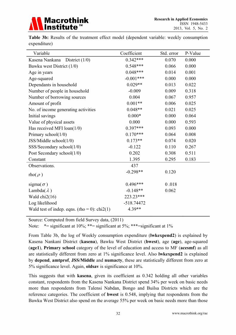
Table 3b: Results of the treatment effect model (dependent variable: weekly consumption expenditure)

Variable Coefficient Std. error P-Value

Kasena Nankana District (1/0) 0.342*** 0.070 0.000 Bawku west District (1/0) 0.548*** 0.066 0.000 Age in years 0.048*** 0.014 0.001 Age-squared -0.001*** 0.000 0.000 Dependants in household 0.029** 0.013 0.022 Number of people in household -0.009 0.009 0.318 Number of borrowing sources 0.004 0.067 0.957 Amount of profit 0.001** 0.006 0.025 No. of income generating activities 0.048** 0.021 0.025 Initial savings 0.000* 0.000 0.064 Value of physical assets 0.000 0.000 0.593 Has received MFI loan(1/0) 0.397*** 0.093 0.000 Primary school(1/0) 0.170*** 0.064 0.008 JSS/Middle school(1/0) 0.173** 0.074 0.020 SSS/Secondary school(1/0) -0.122 0.110 0.267 Post Secondary school(1/0) 0.202 0.308 0.511 Constant 1.395 0.295 0.183 Observations. 437

rho( ) -0.298** 0.120

sigma( ) 0.496*** 0 .018 Lambda( ) -0.148** 0.062 Wald chi2(16) 223.23*** Log likelihood -518.74472 Wald test of indep. eqns. (rho = 0): chi2(1) 4.39**

Source: Computed from field Survey data, (2011) Note: *= significant at 10%; **= significant at 5%; ***=significant at 1%

From Table 3b, the log of Weekly consumption expenditure (lwkexpend2) is explained by Kasena Nankani District (kasena), Bawku West District (bwest), age (age), age-squared (age1), Primary school category of the level of education and access to MF (acesmf) as all are statistically different from zero at 1% significance level. Also lwkexpend2 is explained by depend, amtprof, JSS/Middle and numacty, these are statistically different from zero at 5% significance level. Again, oldsav is significance at 10%.

This suggests that with kasena, given its coefficient as 0.342 holding all other variables constant, respondents from the Kasena Nankana District spend 34% per week on basic needs more than respondents from Talensi Nabdan, Bongo and Builsa Districts which are the reference categories. The coefficient of bwest is 0.548, implying that respondents from the Bawku West District also spend on the average 55% per week on basic needs more than those


2013, Vol. 5, No. 2


from Talensi Nabdan, Bongo and Builsa Districts which are the reference categories. However respondents from the Bawku West District spend about 21% per week more than their counterparts in the Kasena Nankana District. Thus the Bawku West and the Kasena Nankana District contribute to increased consumption expenditure for the respondents in these two Districts as opposed to the other three Districts contribute to respondents from those Districts.

Both the Kasena Nankana and Bawku West districts have very vibrant market centres with patronage from neighbouring country Burkina Faso. It is possible that products of the agro-processors in these two Districts enjoy good demand from their respective market leading to high profits which is ultimately translated into high consumption levels. This finding therefore concurs with Kiiru & Mburu (2006), where it was argued that microfinance can not improve welfare unless there is effective demand for goods and services, which ensures that the products of micro-entrepreneurs are consumed. These Districts have also had numerous MFIs particularly the Bawku West District. This could explain the reason why that District has such high percentage consumption expenditure per week (55%).

The results also showed that the coefficient of acesmf is (0.397) showing a positive relationship with weekly consumption expenditure. This therefore indicates that beneficiaries of MFIs loans spend on the average 40% higher than non-beneficiaries of MFIs loans in the Upper East Region of Ghana holding all other factors constant. This means that benefiting from MFIs loans has the effect of increasing weekly consumption expenditure on basic needs on the average by 40%. As women receive loans from MFIs, these women invest the loans in viable economic activities. This in turn generates (higher) profits or additional incomes which enable them to spend such incomes on their basic needs, thus helping to pull them out of poverty. Again given the fact that beneficiaries of MFIs loan also receive other training in business acumen which enhances their efficiency to better manage their businesses and as such help improve upon their earnings. This finding is consistent with findings from Khandker (1998), which indicated that microfinance reduces poverty by increasing per capital consumption among programme participants and their families. Poverty reduction estimates based on consumption impacts of credit showed that about 5% of programme participants can lift their families out of poverty each year by participating and borrowing from microfinance programmes. Again the results collaborates with the findings of Morduch (1998), which found that households served by the Grameen Bank who were ordered by the amounts they borrowed from the programme, the top quarter enjoys 15% higher consumption per capita than households in the bottom quarter. Also Pitt and Khandker (1998), found that on average, a loan of 100 taka to a female borrower, after it is repaid, allowed net consumption increases of 18 taka, thus also collaborating with the results in this study.

The age coefficient is given as 0.0477, suggesting that if one’s age increases by an additional year, then weekly consumption expenditure will also increase on the average by 5%. Thus as one ages overtime, she becomes more experienced and skilful in her economic activity and this could increase her efficiency level and for that matter higher earnings which is ultimately translated into increased consumption expenditure per week. However, beyond the age of 43 years weekly consumption expenditure declines with an increase in age given the fact that the


2013, Vol. 5, No. 2


coefficient of age-squared (age1 (-0.000556)) is negative. By implication as one ages over and above the age of 43 years, her capacity to garner more resources for consumption begins to wane, thus her weekly consumption level reduces marginally by 0.000556 with an additional increase in age. This has the tendency of increasing poverty levels particular among the aged in the rural areas. The negative impact of this on weekly consumption expenditure may be insignificant though; this could be due to the fact that individuals above 43 years could be receiving remittances from their relatives to augment their consumption expenditure.

The amount of profit per month (amtprof), is also positively associated with weekly consumption expenditure given its coefficient of 0.00134. Thus if profit increases by one cedis (Gh¢1) per month then weekly consumption expenditure will increase by 0.13%. As the respondents make more profits from their agro-processing business they spend part of these profits on basic needs and for that matter driving them out of poverty. Women engage in off-farm economic activities including agro-processing in other to generate additional income. Such incomes are expended on basic needs so as to bridge the household consumption gap and this contributes to poverty reduction within the household. Therefore as profits increase consumption expenditure also increase. The impact of the amount of profit on weekly consumption expenditure is not that substantial.

Again primary school and JSS/ Middles school categories of the level of education both have positive impact on weekly expenditure and for that matter poverty reduction given their coefficients as 0.170 and 0.173 respectively. Thus respondents with primary school and JSS/Middle school education spend on the average 17% and 17.3% respectively higher on consumption per week than their counterparts who have no formal education. From Table 1, given the mean value of the various categories of education, the number of respondents within each category is computed as; no formal education are 232; primary school education are 102 and JSS/Middle school education are 66. Thus the number of respondents with primary and JSS/Middle school education combined is 168; this number is less than those with no formal education which is the reference category. This suggests that may be those with primary and JSS/Middle school education are better able to manage their agro-processing businesses very well and so make more money which enables them to spend on consumption more than those with no education.

The coefficient of the number of dependants in a respondent’s household (depend) is given as 0.0294. This shows a positive relationship with weekly consumption expenditure. Thus as the number of dependants in the household increases by one, weekly consumption expenditure increases on the average by 3%. Possible explanation to this finding is that, the higher the number of dependants in the household, the more the need for respondents (providers) to generate more resources or income for consumption expenditure. Again the more dependants there are in the household, the greater the compelling demand for the women to engage in an off-farm or participate in an MFI programme that enables them generate additional income for consumption expenditure. This finding is contrary to Imai, Arun & Annim (2010) who instead used dependency ratio and found a significant but negative relationship with poverty proxied by Index Based Ranking (IBR) score. It is also


2013, Vol. 5, No. 2


possible that households engage their dependants particularly older ones in their production activities, thus contributing to household labour and helping to generate more income for the household consumption expenditure. If this is so, then the more the number of dependants in the household the higher the consumption expenditure will be and the vice-versa.

Moreover the number of income generating activities that the respondent engages in (numacty) is positively associated with weekly consumption expenditure. Given a coefficient of 0.0479, it suggests that if numacty increases by one then weekly expenditure on basic needs will increase on the average by 5%. It is not surprising that the respondents engage in multiple income generating activities, perhaps the old adage of not putting all eggs in one basket holds here. The region has just one rainy season. Thus off-farm income generating activities may be contributing substantially to their sustenance hence the motivation to engage in multiple income generating activities.

Again oldsav is positively associated with weekly consumption expenditure with a coefficient of 0.000381. By the coefficient as the amount of initial savings increases by GH¢1 then weekly consumption expenditure will increase by 0.04%. Though this may be negligible, it is an indication that respondents who are able to mobilise more savings channel these money into their income generating activities therefore enabling them earn more money for their consumption expenditure. Also initial saving may be a criterion for grant of MFI loans. If this is the case those who are able to mobilise more savings get more loans for their economic activities which also helps them spend much more in the future.

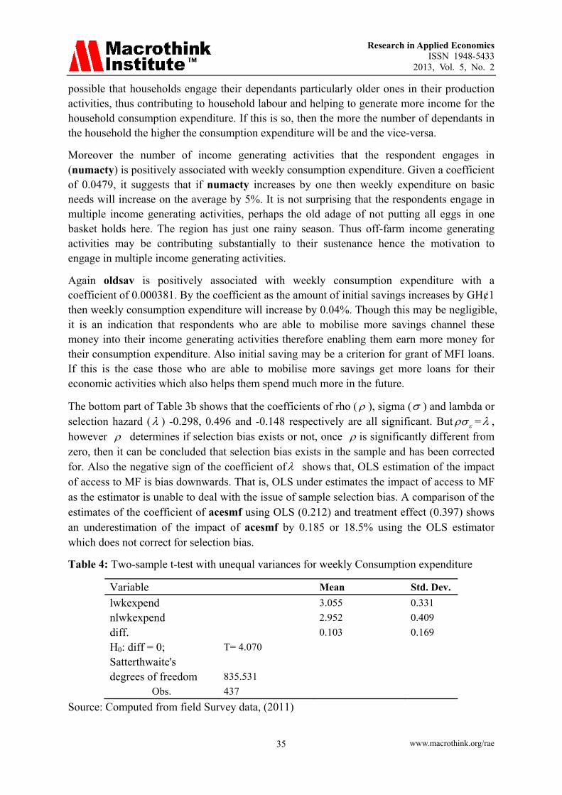
The bottom part of Table 3b shows that the coefficients of rho ( ), sigma ( ) and lambda or selection hazard ( ) -0.298, 0.496 and -0.148 respectively are all significant. But = , however determines if selection bias exists or not, once is significantly different from zero, then it can be concluded that selection bias exists in the sample and has been corrected for. Also the negative sign of the coefficient of shows that, OLS estimation of the impact of access to MF is bias downwards. That is, OLS under estimates the impact of access to MF as the estimator is unable to deal with the issue of sample selection bias. A comparison of the estimates of the coefficient of acesmf using OLS (0.212) and treatment effect (0.397) shows an underestimation of the impact of acesmf by 0.185 or 18.5% using the OLS estimator which does not correct for selection bias.

Table 4: Two-sample t-test with unequal variances for weekly Consumption expenditure

Variable Mean Std. Dev.

lwkexpend 3.055 0.331

nlwkexpend 2.952 0.409

diff. 0.103 0.169

H0: diff = 0; Satterthwaite's degrees of freedom

Obs.

T= 4.070

835.531

437

Source: Computed from field Survey data, (2011)


2013, Vol. 5, No. 2


Note: diff = mean(lwkexpend) - mean(nlwkexpend)

Table 4 shows the t-test of the significance of the difference of weekly consumption expenditure of beneficiaries (lwkexpend) and non-beneficiaries (nlwkexpend) of MFI loans estimated at the means contingent on all the variables that are significant in explaining weekly consumption expenditure as discussed from Table 3b above (Kasena, Bwest, oldsav, amtprof, depend, age, age1, numacty, Primary school, JSS/Middle and acesmf). Thus lwkexpend is mean of log consumption expenditure for beneficiaries contingent on the above variables, nlwkexpend, mean of log weekly consumption expenditure for non- beneficiaries contingent on the above variables while diff is the difference between lwkexpend and nlwkexpend. The mean weekly consumption expenditure for beneficiaries of MFI loans is 3.055 while that of non-beneficiary is 2.952, contingent on all the statistically significant variables.

Taking the anti-log these figures mean that beneficiaries of MFI loans spend about GH¢21.22 per week on basic needs while non-beneficiaries spend GH¢19.14 per week on basic needs contingent on these statistically significant variables. However, the difference between the mean weekly consumption expenditure for the two groups is GH¢1.11. The t-test of the null (H0) that the difference in weekly consumption expenditure for the two groups is equal to zero is rejected given the t-test value of 4.0701. This indicates that beneficiaries spend GH¢1.11 more per week on basic needs than non-beneficiaries.

Using the non-beneficiaries consumption expenditure (nlwkexpend) as a counterfactual outcome for the beneficiaries consumption expenditure (lwkexpend) therefore, it can be said that beneficiaries would have been spending GH¢19.14 per week on basic needs if they had not benefited from the MFI loans; but they now spend GH¢21.22 per week on basic needs, that is GH¢1.11 per week more. This suggests that MF has increased beneficiaries’ consumption expenditure by GH¢1.11 per week on basic needs. By implication access to MF contributed to poverty reduction.

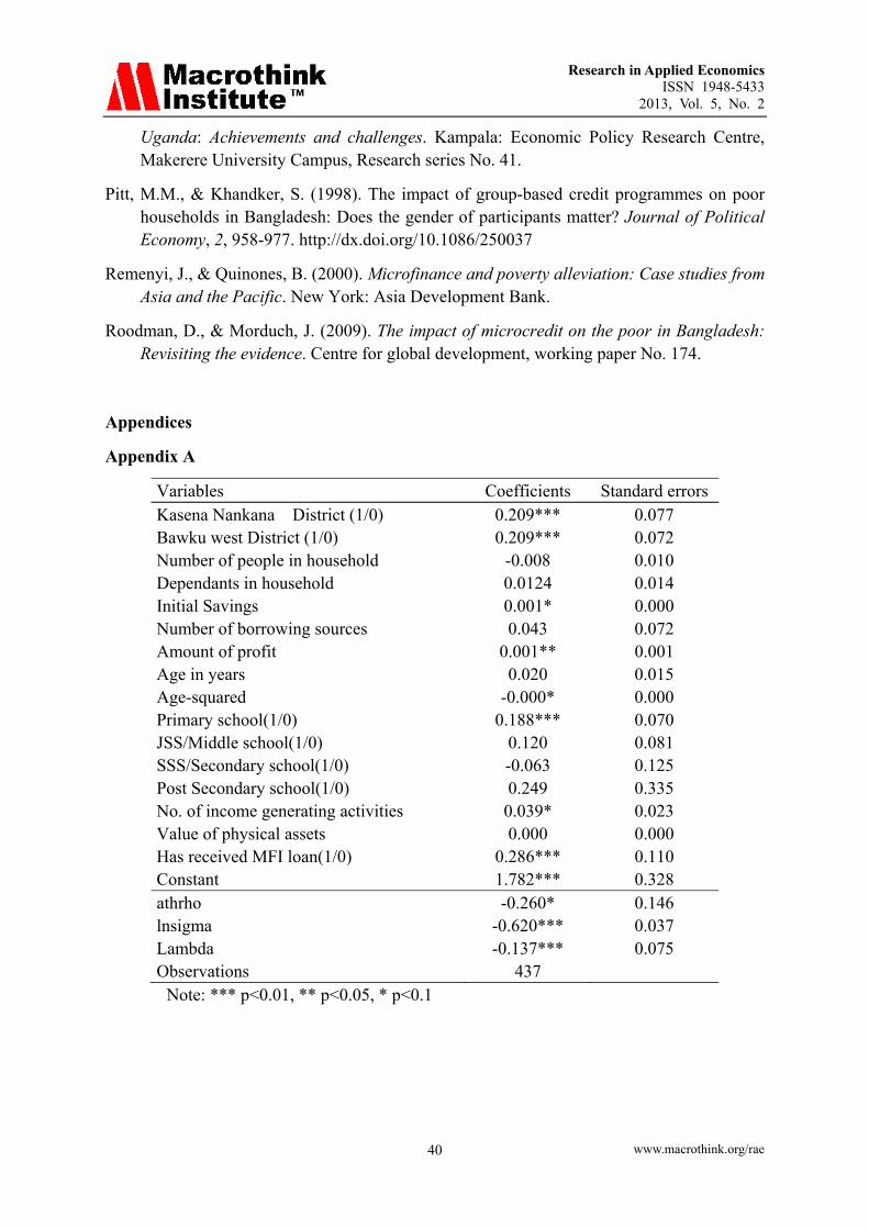
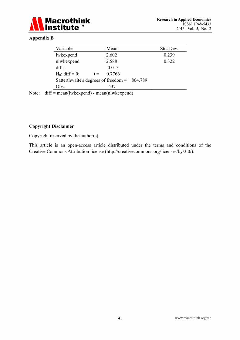
As a robust check weekly consumption expenditure on food was used as a proxy for poverty. Food is seen as the most basic need of life. See appendix A for the results of the treatment effect with the log of consumption expenditure on food (lexpfood) as the dependent variable. The results indicate that kasena, bwest, oldsav, amtprof, age1, primary school education, numacty and acesmf are all significant in explaining consumption expenditure on food. The coefficient of acesmf is given as 0.286 suggesting that beneficiaries of MFI loans spend on the average 29% per week on food more than non-beneficiaries of MFI loans. This is about 11% less than the weekly expenditure on basic needs (0.397) for beneficiaries holding all other variables constant. The mean of log weekly consumption expenditure on food for beneficiaries contingent on the above variables is was found to be 2.602 (260%) while that of non-beneficiaries is given as 2.587(258.7%).

The difference between the mean weekly consumption expenditure on food for the two groups is given as 0.015 (0.15%) contingents on all the statistically significant variables. The t-test of the null (H0) that the difference in weekly consumption expenditure for the two groups is equal to zero is not rejected given the t-test value of 0.777. This indicates that there


2013, Vol. 5, No. 2


is no marked difference in consumption expenditure on food for beneficiaries and non-beneficiaries of MFI loans. By this therefore, beneficiaries of MF would have been spending the same amount weekly on food even if they had not received MF and for that matter access to MFI loans have no impact on food consumption. See appendix B for the results of the Two-sample t-test with unequal variances for Weekly consumption expenditure on food.

This could be so because in the Upper East Region about 80% of the population are farmers who produce basically for domestic consumption and only sell some into the market if there is surplus food stuff. Thus households are able to produce substantial amount of food for their consumption. They may also spend some amount of money on food from the market to meet short falls in domestic production. Thus whether one receives MF or not, they must endeavour to meet their food consumption requirements as much as possible.

5. Conclusions and Policy Recommendations

The study sought to evaluate the impact of access to microfinance on poverty reduction proxied by consumption expenditure on basic needs. The treatment effects estimation model was employed to solve the problems of selection bias and endogeneity. From the results and findings the conclusions from the study are that:

Respondents from the Kasena Nankani and Bawku West Districts have less probability of accessing or taking loans from MFIs than their counterparts from the Talensi-Nabdan, Bongo and Builsa Districts which are the reference categories. Again the amount of initial savings and the number of sources of borrowing that the respondent can actually borrow from within the community when in need of a loan reduce the probability of participating in an MFI programme and for that matter taking a loan from an MFI. Also the amounts of profit respondents make in a month and the number of friends of the respondent who have ever borrowed from an MFI increase the probability of participating in MFI programmes and for that matter taking a loan from an MFI. Also, Kasena, Bwest, oldsav, amtprof, depend, age, age1, numacty, Primary school, JSS/Middle are the variables that are significant in explaining consumption expenditure.

The implications are that respondents from districts without vibrant market centres have higher probability of accessing micro-credit from microfinance institutions. Again access to microfinance by rural women contributes positively to consumption expenditure and for that matter poverty reduction among the rural households in the Upper East Region.

It is therefore recommended that MFIs should endeavour to reach out to more rural women engaged in agro-processing. MFIs should lend out loans to more clients in Districts with very vibrant market centres. Also microfinance investment is recommended to broaden the scale and scope of beneficiaries reached and improve delivery strategies to suite context specific characteristics.


2013, Vol. 5, No. 2


References

Annim, S. K. (2009). Targeting the Poor versus financial sustainability and external funding: Evidence of microfinance institutions in Ghana. Brooks World Poverty Institute, University of Manchester, BWPI Working Paper 88.

Banerjee, A., Duflo E., Glennerster R., & Kinnan C. (2009). The miracle of Microfinance? Evidence from a randomised evaluation. Cambridge, MA: Department of Economics, MIT, Mimeo.

Binswanger, H. P., & Khandker S. R. (1995). The impact of formal finance on rural economy of India. The Journal of Development Studies, 32(2), 234-262. http://dx.doi.org/10.1080/00220389508422413

Consultative Group to Assist the Poor (CGAP) (2008). Who is funding Microfinance? Results of the First Global Survey of Funders Microfinance Portfolio. Washington DC:

Duvendack, M., Palmer-Jones, R., Copestake, JG., Hooper, L., Loke, Y., & Rao, N. (2011). What is the evidence of the impact of microfinance on the well-being of poor people? London: EPPI-Centre, Social Science Research Unit, Institute of Education, University of London. ISBN: 978-1-907345-19-7

Feigenberg, B., Field, E. M., & Pande, R. (2010). Building social capital through microfinance. Kennedy School, Harvard University, Cambridge. http://dx.doi.org/10.3386/w16018

Ghalib, A. K., Malki, I., & Imai, K. S. (2011). Impact of microfinance and its role in easing poverty of rural households: Estimation from Pakistan. Discussion paper series no. DP2011-28, Kobe University, Japan, Research Institute for Economics and Business Administration.

Ghana Statistical Service. (2008). Ghana living Standard survey: Report of Five Round (GLSS5). Accra: Author

Gobezie, G., & Garber, C. (2007). Impact assessment of the microfinance programme in Amhara Region of Ethiopia. Paper presented at International Conference on Rural Finance Research: Moving Results into Policies 19-21 March 2007 FAO Headquarters, Rome Italy.

Heckman, J. (1979). Sample selection bias as a specification error. Econometrica, 47, 153–161. http://dx.doi.org/10.2307/1912352

Heckman, J. J., & Vytlacil, E. (2005). Structural equations, treatment effects, and econometric policy evaluation. Econometrica, 73(3), 669-738. http://dx.doi.org/10.1111/j.1468-0262.2005.00594.x

Hulme, D. (n.d.). Impact assessment methodologies for microfinance: Theory, experience and better practice. Manchester: Institute for Development Policy and Management, University of Manchester.


2013, Vol. 5, No. 2


IFAD, (2000). Ghana- Women’s access to formal financial services. Retrieved February 12, 2010, from http://www.ifad.org/gender/learning/sector/finance/42.htm

IFAD, (2004). Investing in Microfinance. Retrieved February 12, 2010, from http://www.ifad.org/events/yom/what.htm

Imai, K.S., Arun, T., & Annim, S.K. (2010). Microfinance and household poverty reduction: New evidence from India. Discussion paper series no. DP2010-14, Kobe University, Japan, Research Institute for Economics and Business Administration.

Imai, K.S., & Azam S. (2010). Does microfinance reduce poverty in Bangldesh? New Evidence from household panel data. Discussion paper series no. DP2010-24, Kobe University, Japan, Research Institute for Economics and Business Administration.

Karlan, D., Harigaya, T., & Nadel, S. (2006). Evaluating microfinance programme innovation with randomized controlled trials: Examples from business training and group versus individual liability. Retrieved October 15, 2010, from http://www.microcreditsummit.org/papers/Workshops/8_Karlan.pdf

Karlan, D. & Zinman J. (2009). Expanding credit access: Using randomised supply decisions to estimate the impacts. New Haven, Financial Access Initiative.

Khandker, S. R. (1998). Fighting poverty with microcredit, experience in Bangladesh. Oxford: Oxford University Press.

Khandker, S. R. (2005). Microfinance and Poverty: Evidence Using Panel Data from Bangladesh. The World Bank Economic Review, 19(2), 263-286. http://dx.doi.org/10.1093/wber/lhi008

Kiiru J. M. (2008). Microfinance, Entrepreneurship and Rural Development: Empirical Evidence from Makueni District, Kenya. Centre for Development Research (ZEF) Bonn University, Germany.

Kiiru, J., & Mburu, J. (2006). User costs of joint liability borrowing and their effect on livelihood assets for rural poor households. International Journal of Women, Social Justice and Human Rights, 9, 14-263.

Morduch, J. (1998). Does microfinance really help the poor? New evidence from flagship programmes in Bangladesh. New York: Department of Economics. Retrieved October 08, 2009, from http://www.nyu.edu/projects/morduch/documents/microfinance/Does_Microfinance_Really_Help.pdf

Morduch, J. (1999). The microfinance promise. Journal of Econometric Literature, 37, 1569–1614. http://dx.doi.org/10.1257/jel.37.4.1569

Morduch, J., & Haley, B. (2002). Analysis of the effects of microfinance on poverty reduction. New York University Wagner Working Paper No. 1014.

Okurut, F. N., Banga, M., & Mukungu, A. (2004). Microfinance and poverty reduction in


2013, Vol. 5, No. 2


Uganda: Achievements and challenges. Kampala: Economic Policy Research Centre, Makerere University Campus, Research series No. 41.

Pitt, M.M., & Khandker, S. (1998). The impact of group-based credit programmes on poor households in Bangladesh: Does the gender of participants matter? Journal of Political Economy, 2, 958-977. http://dx.doi.org/10.1086/250037

Remenyi, J., & Quinones, B. (2000). Microfinance and poverty alleviation: Case studies from Asia and the Pacific. New York: Asia Development Bank.

Roodman, D., & Morduch, J. (2009). The impact of microcredit on the poor in Bangladesh: Revisiting the evidence. Centre for global development, working paper No. 174.

Appendices

Appendix A

Variables Coefficients Standard errors Kasena Nankana District (1/0) 0.209*** 0.077 Bawku west District (1/0) 0.209*** 0.072 Number of people in household -0.008 0.010 Dependants in household 0.0124 0.014 Initial Savings 0.001* 0.000 Number of borrowing sources 0.043 0.072 Amount of profit 0.001** 0.001 Age in years 0.020 0.015 Age-squared -0.000* 0.000 Primary school(1/0) 0.188*** 0.070 JSS/Middle school(1/0) 0.120 0.081 SSS/Secondary school(1/0) -0.063 0.125 Post Secondary school(1/0) 0.249 0.335 No. of income generating activities 0.039* 0.023 Value of physical assets 0.000 0.000 Has received MFI loan(1/0) 0.286*** 0.110 Constant 1.782*** 0.328 athrho -0.260* 0.146 lnsigma -0.620*** 0.037 Lambda Observations

-0.137*** 437

0.075

Note: *** p<0.01, ** p<0.05, * p<0.1


2013, Vol. 5, No. 2


Appendix B

Variable Mean Std. Dev. lwkexpend 2.602 nlwkexpend 2.588 diff. 0.015 H0: diff = 0; t = 0.7766 Satterthwaite's degrees of freedom = 804.789 Obs. 437

0.239 0.322

Note: diff = mean(lwkexpend) - mean(nlwkexpend)

Copyright Disclaimer

Copyright reserved by the author(s).

This article is an open-access article distributed under the terms and conditions of the Creative Commons Attribution license (http://creativecommons.org/licenses/by/3.0/).

access to microfinance by rural women: implications for

Documents